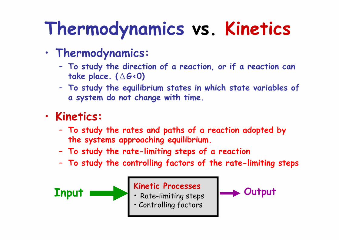
• Thermodynamics:– To study the direction of a reaction, or if a reaction can

take place. (ΔG<0)– To study the equilibrium states in which state variables of

a system do not change with time.

• Kinetics:– To study the rates and paths of a reaction adopted by

the systems approaching equilibrium.– To study the rate-limiting steps of a reaction– To study the controlling factors of the rate-limiting steps

Thermodynamics vs. Kinetics

Input OutputKinetic Processes• Rate-limiting steps• Controlling factors

Thermodynamics vs. Kinetics

Reaction Rate α (Kinetic factor) x (Thermodynamic factor)* Kinetic factor relates to Q (activation energy), while the thermodynamic factor relates to the driving force, ΔG=G2-G1.

* The thermodynamic factor decides the direction of a reaction, while the kinetic factor, the rate of reaction.

G1

G2

Initial Activated FinalState State State

Q

ΔG

Kinetic theory: The reaction rate is proportional to the probability to reach activated state that follows the Arrheniusrate equation, exp(-Q /RT).

* The activation energy (Q) can be obtained from the slope of curve plotted as ln (reaction rate) vs. 1/T

Example: For diamond growth by CVD from reaction of methane and hydrogen

- Q/R

Kinetic factor increased by changing temperature or adding catalysts.

Examples: (1) N2 + 3H2 = 2NH3 using iron as a catalyst(2) 2CO + 2NO = 2CO2 + N2 using Pt and Rh as

catalysts for catalytic converters used in automobile

Activation energy (Q) without catalyst

Activation energy (Q) with catalystReactants

Products

Free

Ene

rgy

Progress of Reaction

ΔG<0

Examples: Thermodynamically favorable but kinetically unfavorable phase changes

(1) Is a diamond forever?

Diamond GraphiteDiamond

Liquid

Vapor

Graphite

0 2000 4000 6000Temperature (K)

1011

109

107Pres

sure

(Pa

)

Diamond

Graphite

Free

Ene

rgy

Progress of Reaction

ΔG=-2.9KJ/mol

Very large Q

(2) Crystallization of glasses

Supercooledliquid

Shrinkage due to freezing

50m

1 h

2 h

8 h

CaO-SrO-BaO-B2O3-SiO2 glass-ceramics annealed at 875oC

Pseudowollastonite(Ca,Ba,Sr)SiO3

Cristobalite SiO2

Diffusion driven by decrease in chemical potential

Free energy of diffusion couple = G3Diffusion taking place to homogenize to obtain G4

μ1B>μ2

BB diffusing from (1)→(2)

μ2A>μ1

A A diffusing from (2)→(1)

Down-hill Diffusion

* Down-hill diffusion

G1G2 G3

G4

A 2 1 B

μ2A

μ1A

μ1B

μ2B

2 1

AB

μ1B<μ2

BB diffusing from (2)to (1)

μ2A<μ1

A A diffusing from (1)to (2)

Up-hill Diffusion

* Up-hill Diffusion

A 2 1 B

G3

G4

G1G2

μ2A

μ1A μ2

B

μ1B

2 1A

BFree energy of diffusion couple = G3Diffusion taking place to homogenize to obtain G4

( )

v ( ) ( )

: , :

CDriving force notx x

J C C B F C Bx

B Mobility F Force

Diffusion:Process by which matter is transported through matter as a result of molecular motions

General scheme for transport phenomena

Flux α Driving force α Gradient in potentialMatter J α dC/dx α Concentration potentialHeat q α dT/dx α Temperature potentialElectricity I α dψ/dx α Electrical potential

: thermal c

: electrical conduc

: diff

onductivi

tivity

t

usivit

y

y

( ' )( ' )

( ' )

D

k

J D C Fickq k T Fourier s LI Oh

s La

m s Law

w

aw

time

Fick’s First Law:Species migrates from a region of high concentration to a region of low concentration；in general the rate of diffusion is proportional to the concentration gradient

CJ Dx

* Flux (J) : Mass/(area‧time), e.g., g/(cm2‧sec)

* Minus (-): Matter moves from high to low concentration.

* Diffusivity (D): Diffusivity related to atomic mobility and crystal structure, e.g., cm2/sec (independent of concentration gradient)

* Concentration gradient ( ): Gradient in ”Mass Potential,”e.g., g‧cm-3/cm

Cx

0( )xCt

( )C C x

Steady State:

Concentration at a given point is invariant with time

i.e.,

J≠J(x,t) when area is fixed

Key: to describe C(x,t) quantitatively

H

Time

Transient State

t = ∞

X=0 X=LCo

ncen

trat

ion

Steady State

Ceq

x x xoo

CSteady State Solution :C( ) = A + B = C -L

Steady State: Constant flux if the area is fixed.

Equilibrium State: No Flux

μ: Chemical Potential

( ) 0 ( )t tC

x x

( ) 0 ( )x xC

t t

RT ln ( ) RT ln( )

ln( ) ln( )( ) RT( ) RT( )t t t

a X

a X

x x x

Steady State:

area is fixed

Under any conditions

when D is constantC Cx x

22( ) 0t

Cx

( ) 0xC

t

( ) 0tJ

x

x

x

J1

No Depletion or Accumulation

C

C

J

t

J1

( ) 0xCt

Fick’s Second LawTransient State: C=C(x,t), or J=J(x,t)

2 2

2 ........2!x x x

J J dxJ J dxx x

From Taylor Series

JXJX+ΔX

X X+ΔX

A (area)accumulation or depletion of concentration exists

Mass Conservation

x x xm CJ A J A A xt t

Flux · Area = Rate of change of concentration · volume(g cm-2sec-1· cm2 = g cm-3sec-1 · cm3)

(A is fixed)

x x+Δx

Jx Jx+Δx

( )

x xJ CJ A J dx A A xx t

J Cdx A A xx t

Fick’s Second Law (cont.)

( )C J CDt x x x

2

2

C C DDx x x

2

2 ( )C C D CDx x C x

when ( ) 0DD D CC

2

2

C CDt x

Linear partial differential equationSolutions are additiveSolutions require initial and boundary conditions

Fick’s Second Law

C

x

( )D D CSteady State

Transient State:

( ) 0tJ

x

x

x

2

2

C J CDt x x

22( ) 0t

Cx

If J2<J1 Accumulation

t( ) 0x

Ct

J1

Depletion or Accumulation

C

C

J

J2

C*

2δ

Transient State --Thin-film solution (Infinite Sink)

A quantity of solute, S, is plated as a thin film on one end of a long rod of solute-freematerial, then a similar solute-free rod is welded to the plated end.

t

2

2C CFick's 2nd Law : =D

x

I.C. C(x,0)= 0 |x|>δC(x,0)= C* |x|≤δ

B.C. C(∞,t)=0C(-∞,t)=0

Annealed for time (t) Determine concentration profile of the solute.

Assuming D ≠ D(x) (Constant diffusivity)

-3 -2 -1 0 1 2 3

X (Distance)

C/S’

2.0

1.5

1.0

0.5

0

Dt=00.025

0.05

0.075

0.25

1.0

3.0

' 2

( , ) exp( )42

S xC x tDtDt

Transient State --Thin-film solution (Infinite Sink)

Time

' *( , ) ( 2 )C x t dx S C

2

( , ) exp: ( )4

A xC xGeneral So tDtt

lution ' 2

(Note: 2 ): ( , ) exp( ) 42

DtS xC x t

DtDtParticular Solution

'

(0, )2

SC tDt

2

( , ) (0, ) exp( )4xC x t C tDt

2Thus a graph of ln( ( , ) (0, ) ) against x should yield a straight line with a slope of 1 4 .

C x t C tDt

Conservation of mass

S’= g/cm2 (Surface Concentration)C*= g/cm3

Taking the natural logarithm of both sides yields2( , )ln( )

(0, ) 4C x t xC t Dt

(A: constant)

2( , )ln( ) .(0, )

C x tif vs xC t

is not a linear relation, D is a function of concentration. If it is linear, D is independent of concentration.

' 2

( , ) exp( )42

S xC x tDtDt

0(1) | 0 Impermeable Boundary

' 1(2) (0, ) (0, )2

x

SC t

C

C tDt

x

t

2

(3) 1 24

' (0, )( , ) exp( 1) this plane is determined.2

( 2 ) 0.

xwhen x DtDtS C tC x t

eDtx t this plane x Dt moves away from x

-1/4Dt

x2

ln[C

(x,t)

/C(0

,t)]

Determine D

Thin Film Solution

CJ=-D x

22

∂C ∂ C=D∂t ∂x

∂C∂x

MaximumDepletion

22

∂ C∂x

C

X=0 X

(a)

(b)

(c)

ZeroAccumulation

-J +JJ=0

Maximum Flux

Leak Test

0

0.2

0.4

0.6

0.8

1

1.2

-6 -4 -2 0 2 4 6-∞ - l 0 l ∞

Sample Dimension

The above analyses are only good for a thin film in the middle of an “Infinite Bar”. If it is not infinite, the diffusion will be reflectedback into the specimen when it reaches the end of the bar, and concentration in that region will be higher than the above solution.Q: How long is long enough to be considered infinite?Leak TestArbitrarily taking 0.1% as a sufficiently insignificant concentration

' 2

0

' 2

3

0( , ) exp( )

4

exp( )( , ) 420.1

2

,2 2

% 1

2

0l

l

x dxLet u duDt Dt

x ulx l uDt

S

S x dxC x

xC x t dx dxDtD

t

t

t dx DtD

'2

3 2'

2

0

exp( )10

exp( )

( )2 1 ( )1 2

lDt

S u du

S u du

lerfclDt erfDt

4.6l Dt

4.6l Dt The bar is considered to be long enoughto use a thin-film solution with 99.9% accuracy.

(Check the Table of Error Function)

Superposition(1) No interaction from adjacent slabs(2) Superposition of the distributions

from the individual slabs since the diffusion equation is linear and additive.

Solution for a pair of Semi-infinite Solids

00

x

CC’

i

. . ( ,0) 0 0 ( ,0) ' 0 . . ( , ) '

( , ) 0

I C C x xC x C x

B C C t CC t

2'

1

2'

0

( , ) exp( )42

0

( , ) exp( )42

ni

i

i

xCC x tDtDt

n

xCC x t dDtDt

C(x,t)

0α2

X

C

Δα

0

* 22( ) /4

2x Dtc e

Dt

2'

'

( , ) exp( )42

:

ii

xCC x tDtDt

Note S C

Sum the solution of all thin slabs

2'

1

2'

0( , ) exp(

( , ) exp )

)

0

4

(

2

42

n

i

i

i

xCC x tDt

xCC x t dDtDt

Dtn

Substituting , 22xu d Dtdu

Dt

C(x,t)

0α2

X

C

Δα

0

* 22( ) /4

2x D tc e

D t

'2

2

02

( , ) exp( )xDt

xuDt

uCC x t u du

reverse limits of integration and split integral

'0 220

( , ) ( ) exp( )xDt CC x t u du

By definition of error function2

0

2( ) exp( )

( ) 1 (0) 0( ) ( )

zerf z u du

erf erferf z erf z

' 0 2 220

'

'

( , ) [ exp( ) exp( ) ]

[ ( )]2 2 2

[1 ( )]2 2

xDtCC x t u du u du

C xerfDt

C xerfDt

1

0 0

0.50

CC

0.5

X

0.50.5 ( )2

xerfDt

0.5 ( )2

xerfDt

(2)

0

0

0

0

0

0

1 [1 ( )]2 2

1(1) 0 0.5 ( )2 21 0 0.5 ( )2 2

(2) 1 0.921 2

which varies with time as 2

(all compositions except 0.5)

(4)

.

1(3) 0 (implicit B.C.)2

x

o

C xerfC Dt

C xx erfC Dt

xCx erfC Dt

x CCDt

x DtC

C

J D

CxC

0

00

0

(5) Total mass crosses the plane a

| (

:to the lef

t 0

(A:a

t)

re

2

a)

x

t

C

M Dt

C D

C

x

tA

tx

Jd

-

Note: If the concentration is fixed (C=C*), the term of is then also fixed. This means that the penetration distanceis a function of the square root of

the diffusion time. For example, if a diffusion penetration of 0.1mm develops in one hour, it will take 4 hours to develop a penetration of 0.2 mm.

/ 2x Dt

The above analyses are only good for an “Infinite Slab”. If it is not infinite, the diffusion will be reflectedback into the specimen when it reaches the end of the bar, and concentration in that region will be higher than the above solution.

Q: How long is long enough to be considered infinite?Leak TestArbitrarily taking 0.1% as a sufficiently insignificant concentration

0

3

00

01 [1 ( )

1( , ) [1 ( )]2

](

2

, ) 2 20.1% 10l

l

xC erf dxC x tx

dx DtC x t dx C erf dx

Dt

Co

0 l

time

time

0 X0

1

0.5CCo

t∞

'( , )'( , ) 0

2'( , ) [1 ( )]

2 2

( , ) ( )2

C t C A BCC t A B A B

x

C xC x t erf

C x t A

D

e

t

B rfDt

Using B.C. to solve the problem

Examples

(1) if C(0, t) = 0 '( , ) ( )2

xC x t C erfDt

(2) if C(0, t) = C”=A, C(∞,t)=C’"( , ) [1 ( )], 0

2xC x t C erf xDt

" ( ), 0' " 2

C C xerf xC C Dt

(next page)

Error Function & its Derivatives

Note: (2) is the thin film solution

xx

x

xx

xx

≡

≡3

3

2

2d (er

(1) erf(

f( ))(3) Accumulation

d(erf( ))(2) (-)Fl

d (erf(

u

))(4)

xd

d

)

d

(1)

(1)(2)

(3)

(4)

Diffusion from a Limited Source (thin film)

00

20

( , ) constant

( , ) exp( )4

(0, ) constant

C x t dx S

S xC x tDtDt

C t

:Gaussian function

Example: p-n junctionC’= Background Concentration

'

2' 0

( )

junction distance

exp( )4

j

j

C C p n or n p

x

xSCDtDt

t1 t2 t3 t4

X

Co

C'

t1<t2<t3<t4

x

-0.2

0

0.2

0.4

0.6

0.8

1

1.2

1.4

1.6

1.8

2

0 0.5 1 1.5 2 2.5 3

C’

x

Time

xj

Diffusion from a Constant Source

00

0

0

( , ) ( )2

(0,

( )

)

, 2

xC x t C e

DtM A C x t dx AC

C

cD

t

rft

C

: the amount of dopant entering the base

Example: p-n junctionC’= Background Concentration

'

'0

( )

: junction distance

e ( )2

j

j

C C p n or n p

x

xC C rfc

Dt

t1 t2 t3 t4

Co

C’

x

t1< t2< t3< t4

xj

Series SolutionsSmall system + long timeReal solution to all systems without assumptions of “Infinite System”

Assuming the solution can be represented by

2

2

'

2

2

( , ) ( ) ( )

assum ing ( )

( ) ( ) "

dT D Td

C x t x T tC CD D D Ct x

x T t Dt x

T

Separation of Variables

x/h

C/Co

Time

-5 -4 -3 -2 -1 0 1 2 3 4 5

1.0

0.5

0

' "

'

"

"

:

:

( , )

TDT

Divide both sides by C x tdT

DTdtT T

TDT

functio

function onl

n o

y o

nly

f di

of

st

time

ance

20

2

ex

1

p( )

dT DT dtT T Dt

where T0 is a constant, -λ2 is chosen because one deals with the systemin which any inhomogeneities disappear as time passes, i.e., T approaches zero as time increases.

Since they vary independently, both sides must be equal to a constant, designated as -λ2 where λis a real number

22 0d

dx

x

The equation in is

the solution to this equation is of the form'( ) sin( ) cos( )x A x B x

where A’ and B’ are functions of λ

2 '0

2

( , ) ( ) ( )exp( )( sin cos )

( sin cos ) exp( )

C x t x T tT Dt A x B x

A x B x Dt

But if this solution holds for any real value ofλ, then a sum of solutions with different values ofλ is also a solution. Thus in its most general formthe product solution will be infinite series of the form

2

1( , ) [( sin cos )exp( )]n n n n n

nC x t A x B x Dt

2

1

0

. . ( ,0) 0

(0, ) 0 0 ( , ) 0 the argument of sin is equal to zero

where is a positive integer

( , ) ( sin )(

. . ( , )

exp( ))

( ,0

0

)

0 o

n

n

n

n n nn

B C C x tI C C x C x h

C t Bx and

C h t xn nh

C x t A x

x

Dt

C C

h

x

1

1

sin (0 )

sin( ) ?

n nn

n nn

A x x h

nA x Ah

00 01

Multiplying both sides by s

in( ) and integrate over the rang

sin

e of 0 to determine

( ) sin

( ) s

(

in )h h

n

n

n

p

p x n x p xC dx A dxh h

x x x h Ah

h

0

01

1

sin ( ) sin( )

s

2

in ( ) sin( ) 0h

nn

h

n nn

n x p x

n x p x hn

n p A dx

p A d Ah h

h h

x

Example :”Diffusion out of a Slab”

2

1( , ) [( sin cos ) exp( )]n n n n n

nC x t A x B x Dt

Time

Co

0 h

00 0

000

0 0

0

0

0

0

2 22 sin( ) ( ) cos( ) cos( )

2 20 [cos( ) cos( )] [1 cos( )]

: 04 4: 2 1

4 1( ,

0,1,2......(2 1)

)(2 1)

hh

nh

n

n

j

C Cn x h n x n xA C dxh h h n h n hC Cn n h n

n h h nn even A

C Cn odd j A jn j

The solution Cx tij

s C

2(2 1) (2 1)sin( ) exp( ( ) )j x j Dth h

Note: Each successive term is smaller than the preceding one, and the percentage decreases between terms and increases exponentially with time. Thus after a shorttime has elapsed, the infinite series can be satisfactorily represented by only a fewterms. To determine the error, we compare the ratio of the maximum values of thefirst and second terms (R) 2

2

2

2

83exp( )

100 4.75

(4.75)

R whe

DtR

n h Dt

htD

h

The error in using the first term to represent C(x,t) is less than 1% at all points.

D

t

is not linear

1o

CnC

C

Degassing of MetalsIt is difficult to measure the concentration of gas at various depths, and what is

experimentally determined is the quantity of gas which has been given off or the quantity remaining in the metal. Therefore, the average concentration ( ) is used.

0

202 2

0

1 ( , )

8 1 (2 1)exp( ( ) )(2 1)

h

j

C C x t dxhC j Dt

j h

0( ) 0.8C t CWhen the first term is a good approximation to the solution or when t issufficiently large

2

2

20

: relaxation time

8 exp( )

Large slow process

hD

C tC

(1st term is not a good approximation)

Solutions for Variable D2

2( )C C D C CD Dt x x x x x

Dx

makes this equation inhomogeneous, especially when D=D(C) or D(T) or D(t) or D(x).

The key in solving the above p.d.e. is to simplify the equation with x and t to x or t function.

Boltzman-Matano Analysis (D=D(C))

32

32

12

1

1 ( )2

1 (

(2

)

)

xt

C C x Ct t tC C Cx x t

x C D C

C

x ttCD

Ct

D

and

Therefore

0

00

CxdC

'

' '

' '

''

'

0 0

00

0 0 00

1

( )2

1 |2

| | |2 ( )

C C C

C

C C

C

C

x C dC dCdC D D D tx d

CdC d D

dC

xt d

xdC D

t

tdx

* x=0 is not determined yetIf D≠D(C), C=Co/2 which determines x=0 for an infinite system. However, if D=D(C) the above condition is no longer valid, the x=0 must be determined by

which expresses the equality of the two shaded areas.

Example: Infinite System I.C. C(x,0)=Co x<0η= -∞C(x,0)=0 x>0η= ∞

Original interface

Co

X=0

Co

Equal area

Matanointerface

Time

X=0

Co

Matanointerface

C’

Tangent=(dC/dx)C’

For an infinite system

000 0 | 0C

odC dCwhen C or C Cdx dx

Therefore0

0

0

0

00

0

0

1 |2

| 0

0

C C

C

C

dCxdC Dtdx

dCdx

xdC

which is an additional boundary condition and determines the location of Matano interface.

'

'

0

0

'

0

1( ) ( )2

0C

C

C

dxD C xdCt dC

xdC

x=0 plane (Matano interface) determined by

X=0

Co

Matanointerface

C’

Tangent=(dC/dx)C’

0

:

:

:

S lo p e

D i f fu s iv i t y

A r e a

xx

x x *

1

2

* *

C * *

C * *

C

C

C *

C

*

C

C

>

<

=

∂ C |∂D

d C

∂ C |∂

D

d C

'

''

0

1( ) ( )2

C

CdxD C xdC

t dC

C*

D2D1

C1

C2 Original interface

t =0

C1

C2

Matano interfacet =t

x=0

Areas equal

C1

C2

0

Slope=dC/dx at C*

C**

The Moving Boundary Problem*Diffusion controlling process along with reaction at phase boundary

?dSdt Kinetic Issue

General Aspects

2

2

2

2

* *

.

* C

C

*

* Diffusion controlling process

:partition

and : equ

ratio between

ilibrium concentrations in phases I and II

phaC C

II

CS Dt x

CS Dt x

k

C C

k

x

x

Ⅰ ⅠⅠ

Ⅱ ⅡⅡ

Ⅰ

* *Ⅰ Ⅱ

* *

sesC* ( ) ( ) ( )x S x S

C dSD D C Cx x dt Ⅰ Ⅱ

Ⅰ Ⅱ Ⅱ Ⅰ

xCs

S

II I

C0

CII*

CI*

To have net diffusion flux between and , the thickness of + has to vanish.

Decarburization

orC C

C Ca a

==

Concentration

Tempe

ratu

reFr

ee E

nerg

yCo

ncen

trat

ion

Micro

stru

ctur

e

α

γα+γ

CαCγ

α γ

α γα+γ

CαCγ

α γ

α+γ

x

Cα

Cγ

S

α γ

T1

Carburization: -Fe -FeDecarburization: -Fe -Fe

Decarburizationforming phase at the interface

Carburizationforming phase at the interface

Decarburization

Carburization

T

C (wt%)

γα+γ

Cα* Cγ*

T* γ+Fe3C

910°C

723°C

0.0250.83

Ci1Ci

2

α

xCs

S

α γ

Ci1

Cα*

Cγ*

T=T*

x

Cs

αγ

Ci2

Cα*

Cγ*

T=T*

S

C Cα γμ =μ at x=S

where α and γ coexist

Sx

μc, ac

A: area for diffusion: constant

x x

Mass Conservation

x x

II I

II III I II =S

* *II

I

I

=S

J - J∂C ∂CJ -

( )A dt = (C -C )A dS

J -D ( ) - (-D )∂ ∂

=

S

dS

0

III

CO

C*I

C*II

CS

CarburizationCs

C*

C*

Co

S0 x

T=T*

γ α γ α

known parameters:

?dSdt

* * C CS oC , C , C , C , D and D

2

22

2

4 2

42

2

[ ] ;[ ]

2[ ]

k

c

k

cH

CO C CO

k COa orCO

CH H Ck CHa

P

Example: Carburization

*Rate of advance of boundary controlled by diffusion of carbon in Fe. Therefore

C C

( C C )

x S k

if at x S reaction controlling process

* *

* *

*

*

C C at x S

C C at x S

* Semi-infinite solid( ) C C

CD D C D D

0V mass flux requiring no density correction

*Chemical activity of carbon at surface can be set up by

*

*

*

Fick’s 2nd law

*

2

2

2

2

0

*

0

*

*

*

*

0

.

( ) (

.

)

( ) (

: ( ,0)

. . :

0

( , )

)

( : )

C

C

s

C Cx s x

C CD x St x

C CD x S

t xI C C x C

B C

C C at x S

C C at x

C C at x S

C C at x

C s t C kC k Partitio

in phase

At x S

J J dt C C

in pha

dSC CD Dx x

se

n Ratio

*

* *

*

: ( ) (

)

)

(s

Note J J dt A C C dS A

dSC Cdt

ds

JSolute receiving

Solute entering

J

Cs

C*

C*

Co

S0 x

0

*

0

*

*

*

In phase

( ), 2

In phase

' ' ( ), ; 0 '2

( , ) ( )2

( , ) ' ( )2

At boundary

' ( )2

a

C

sC

C

s C

s C

xC A B erfc x C C AD t

xC A B erf x S C C x C C AD t

xC x t C B erfcD txC x t C B erfD t

x S C C

SC C B erfD t

C

*

nd are constants ( diffusion controlling process)

therefore is a constant too (constant)2 2

2 where is a constan

( , ) ' ( ) ' ( )

t

2

S

C C

C

s sC

C

S SD

SC S t C C B erf C B erfD t

t D t

S D t

Cs

C*

C*

Co

S0 x

*

1 *2

2

2

0

0 0

' 2( ) exp( ) | (1)4

Similarly

Replace

2

2( ) exp( ) | (242

2( , ) (

( , ) ( )

) ( )2 2

CC

x s x sCC

CC

x s x sC

C

C

C C

C

C

DD

C S t C B e

C D B xDx D tD

D tSC S t C C B erfc C B erfcD t D t

rfc C

t

C D B xDx D tD t

2 2

* *

* *

2

(Note: it is not a c

.(1) (2) ( )( )

'

onst

)

ant)

C

C

S D

SEq C Ct

B e BeC C

t

DdSdt t

2 2

*

* ** * 0

1 12

1 *20

2

solve by trial and err

then we get S

or

( ) (

2 an

'

)

(

(

)

d

)s

s

CC

C C C CC Ce erf e e

C B erf C

C Berf

rfc

DdSdt t

c

D t

C

Note: the only unknown parameter in the above equation is β* *

0( , , , , )C CsC C C C D and D are known parameters

Use them to estimate B’ and B, and then to solve β

2

( )e erfc

β

1

0

Example: Decarburization0.4% Carbon Alloy SteelT=800oCCs=0.01% (equilibrium by CO and CO2)t = 30 min S-Fe?

Answer: Co=0.4%, Cs=0.01%C*=0.24%, C*=0.02% (Obtained from Fe-C Phase Diagram)

2 2

**0

8 6 2

1/2

1

*

2

*

2 2

/

1 1

3x10 ; 2x10 cm /sec

66.6

(0.01 0.02) (0.24 0.4)(0.02 0.24)( ) ( )

0.01 (0.24 0.4)0.

0.1

( )(

44 (

) ( )

22( ) ( )

C C

C

C

s

D D

DD

f f

C CC CC Ce erf e

by trial

erf

and error see

c

fF

f

2 0.0 7

)

1 3CS D t c

i

m

gure

*

*0

*2

2* 2

0

*2

02 *

( , )

( ) ( )

( )

exp( )

elimina 1 ( ) exp ) (t ( )e s

II II

IIII x s II

s II

II

II

II

C C er

C S t CC dSD C Cx dt

C C B erf

BC C

B fC C

S

CI*

Cs

Co

723<T<910℃

CarburizationS

CI*

Cs

Co723<T<910℃

De-carburization

S

Fe3c

CI*

Cs

Co

T<723℃

De-carburizationS

+Fe3C

CI*

Cs

CoT>723℃

De-carburization

Formation of a single-phase layer from an initial two-phase mixtureIn the two-phase region, the average composition, Co, is assumed to be uniform, which requires, in effect, that the grain size is small and that second-phase dispersion is uniform.

3α+Fe C