Thermalization time bounds for Pauli stabilizer Hamiltonians · Thermalization in Kitaev’s 2D...
74
Thermalization time bounds for Pauli stabilizer Hamiltonians Kristan Temme California Institute of Technology QEC 2014, Zurich arXiv:1412.2858
Transcript of Thermalization time bounds for Pauli stabilizer Hamiltonians · Thermalization in Kitaev’s 2D...

Thermalization time bounds for Pauli stabilizer Hamiltonians
Kristan TemmeCalifornia Institute of Technology
QEC 2014, Zurich
arXiv:1412.2858


tmix
O(N2e2�✏)

Overview
• Motivation & previous results
• Mixing and thermalization
• The spectral gap bound
• Proof sketch

Thermalization in Kitaev’s 2D model
• Spectral gap bound for the 2D toric code and 1D IsingR. Alicki, M. Fannes, M. Horodecki J. Phys. A: Math. Theor. 42 (2009) 065303

Thermalization in Kitaev’s 2D model
• Spectral gap bound for the 2D toric code and 1D IsingR. Alicki, M. Fannes, M. Horodecki J. Phys. A: Math. Theor. 42 (2009) 065303
� � 1
3e�8�JSpectral gap bound:

Thermalization in Kitaev’s 2D model
• Spectral gap bound for the 2D toric code and 1D IsingR. Alicki, M. Fannes, M. Horodecki J. Phys. A: Math. Theor. 42 (2009) 065303
J. Phys. A: Math. Theor. 42 (2009) 065303 R Alicki et al
Sn
Co
d1
d2
c1
c2
Figure 2. Partitioning Kitaev’s lattice.
The Hamiltonian of the model is
H Kit! = −
!
s
JXs −!
p
JZp, J > 0. (82)
Similarly to the Ising model the ground states are totally unfrustrated: all Xs and Zp haveexpectation 1. This is actually not sufficient to fully determine the state of all spins as the starand plaquette observables are not independent: because of the periodic boundary conditionsthey satisfy
"
s
Xs = 1 and"
p
Zp = 1. (83)
As a consequence, two topological qubit freedoms are left which may be used for encoding.The Hamiltonian (82) can be chosen more generically by multiplying the individual star andplaquette observables by positive but otherwise arbitrary coefficients, this will not changethe set of ground states. Here too, it is natural to consider the commutant of such a genericHamiltonian which consists of a product of two qubit algebras and AXZ. This is seen quiteexplicitly by introducing, similarly to (42), observables for two encoded qubits
X1 ="
j∈c1
σ xj ′ , X2 =
"
j∈c2
σ xj ′
Z1 ="
j∈d1
σ zj , Z2 =
"
j∈d2
σ zj .
(84)
Here, c1, d1, c2 and d2 are the loops shown in figure 1. Unlike for the Ising ring, all qubitobservables are very delocalized.
Let us divide the set of spins into four disjoint subsets, see figure 2: the snake, the comb,spin 1 and spin 2. Spin 1 is located at the crossing of X1 and Z1, i.e. c1 and d1, and similarlyfor spin 2. Note that the qubit X1 has been modified a little, so that it closely follows the snake.
14
� � 1
3e�8�JSpectral gap bound:
Implies mixing time bound:
tmix
O(Ne8�J )

The energy barrier
| 1i| 0i

The energy barrier
tmem ⇠ e�EB
• Arrhenius law
| 1i| 0i
Phenomenological law of the lifetime
Bravyi, Sergey, and Barbara Terhal, J. Phys. 11 (2009) 043029
Olivier Landon-Cardinal, David Poulin Phys. Rev. Lett. 110, 090502 (2013)

The energy barrier
tmem ⇠ e�EB
• Arrhenius law
| 1i| 0i
• Question:Can we prove a connection between the energy barrier and thermalization ?
Phenomenological law of the lifetime
Bravyi, Sergey, and Barbara Terhal, J. Phys. 11 (2009) 043029
Olivier Landon-Cardinal, David Poulin Phys. Rev. Lett. 110, 090502 (2013)

Stabilizer Hamiltonians
Kitaev, A. Y. (2003). Fault-tolerant quantum computation by anyons. Annals of Physics, 303(1), 2–30.
Example : Toric Code
A set of commuting Pauli matrices

Stabilizer Hamiltonians
Kitaev, A. Y. (2003). Fault-tolerant quantum computation by anyons. Annals of Physics, 303(1), 2–30.
Example : Toric Code
A set of commuting Pauli matrices
The Stabilizer Group Logical operators

Stabilizer Hamiltonians
Kitaev, A. Y. (2003). Fault-tolerant quantum computation by anyons. Annals of Physics, 303(1), 2–30.
Example : Toric Code
A set of commuting Pauli matrices
The Stabilizer Group Logical operators
Stabilizer Hamiltonian

Open system dynamics
• Lindblad master equation
⇢ = L(⇢) = �i[H, ⇢] +X
k
Lk⇢L†k � 1
2{L†
kLk, ⇢}+

Open system dynamics
• Lindblad master equation
⇢ = L(⇢) = �i[H, ⇢] +X
k
Lk⇢L†k � 1
2{L†
kLk, ⇢}+

Open system dynamics
• Lindblad master equation
⇢ = L(⇢) = �i[H, ⇢] +X
k
Lk⇢L†k � 1
2{L†
kLk, ⇢}+
• With a unique fixed point

Thermal noise model & Weak coupling limit

Thermal noise model & Weak coupling limit

Thermal noise model & Weak coupling limit
⇢S(t+�t) = trR[e�iH�t(⇢(t)⌦ ⇢R)e
iH�t]The evolution :

Thermal noise model & Weak coupling limit
⇢S(t+�t) = trR[e�iH�t(⇢(t)⌦ ⇢R)e
iH�t]The evolution :
Weak coupling limit & Markovian approximation:
Davies, E. B. (1974). Markovian master equations. Communications in Mathematical Physics, 39(2), 91–110.

The Davies generator

The Davies generator
* Kubo, R. (1957). Statistical-Mechanical Theory of Irreversible Processes. I. General Theory and Simple Applications to Magnetic and Conduction Problems. Journal of the Physical Society of Japan, 12(6), 570–586.Martin, P., & Schwinger, J. (1959). Theory of Many-Particle Systems. I. Physical Review, 115(6), 1342–1373.
For a single thermal bath: KMS conditions*:
Ensures detail balance with:
Gibbs state as steady state
�S↵(!) = e�!S↵(!)�
� / e��HS

Davies generator for Pauli stabilizers
eiHtS↵e�iHt =
X
!
S↵(!)ei!t• Lindblad operators

Davies generator for Pauli stabilizers
S↵(!) =X
!=✏a�✏a↵
�↵i P (a)
eiHtS↵e�iHt =
X
!
S↵(!)ei!t• Lindblad operators
• Syndrome projectors

Davies generator for Pauli stabilizers
• The Lindblad operators are local! (when the code is)
S↵(!) =X
!=✏a�✏a↵
�↵i P (a)
eiHtS↵e�iHt =
X
!
S↵(!)ei!t• Lindblad operators
• Syndrome projectors

Davies generator for Pauli stabilizers
• The Lindblad operators are local! (when the code is)
S↵(!) =X
!=✏a�✏a↵
�↵i P (a)
eiHtS↵e�iHt =
X
!
S↵(!)ei!t• Lindblad operators
• Syndrome projectors

Convergence to the fixed point σ
t > tmix
(✏) ) keLt(⇢0)� �ktr ✏
• For a unique fixed point:

Convergence to the fixed point σ
ketL(⇢0)� �ktr Ae�Bt
t > tmix
(✏) ) keLt(⇢0)� �ktr ✏
• For a unique fixed point:
• Exponential convergence

Convergence to the fixed point σ
t > tmix
(✏) ) keLt(⇢0)� �ktr ✏
• For a unique fixed point:
• Exponential convergence
Temme, K., et al. "The χ2-divergence and mixing times of quantum Markov processes." Journal of Mathematical Physics 51.12 (2010): 122201.

Convergence to the fixed point σ
t > tmix
(✏) ) keLt(⇢0)� �ktr ✏
tmix
⇠ O(�N��1)
• For a unique fixed point:
• Exponential convergence
• A thermal σ implies the bound
k��1k ⇠ ec�N =)
Temme, K., et al. "The χ2-divergence and mixing times of quantum Markov processes." Journal of Mathematical Physics 51.12 (2010): 122201.

Spectral gap bound
20
Definition 13 Given the commuting Pauli Hamiltonian H as in eqn. (1), and for any η ∈2N2 with a Pauli path ηt = ⊕t
s=0αs, we define the energy of the Pauli η as
ϵ(η) = maxt
M!
k=1
2|Jk|ek(ηt)ek(η). (78)
Here ek = ek ⊕ 1 denotes the conjugation of the bit value. In this sum ek and ek areinterpreted as integers. Furthermore, we define the generalized energy barrier as
ϵ = minΓ
maxη∈ 2N
2
ϵ(η). (79)
The minimum is taken over all possible orderings of the qubits Γ.
This definition of the generalized energy barrier differs from the energy cost of an arbi-trary Pauli operator as given in [14] by the factors ek(η) in the summation. These factorsessentially remove any contribution to the barrier that originate from the final Pauli operatorη itself. Therefore the only summands that contribute to ϵ(η) come from violations of gen-erators gi which are not already violated by η itself already. This generalized energy barriercan interpreted as follows:Suppose, we are given a set of commuting Pauli operators G = {gi}i=1,...,M that define
the HamiltonianH . We consider the reduced subset of generators
Gη ="
g ∈ G#
#
#[g,σ(η)] = 0
$
, (80)
which is obtained from removing all generators gi from the generating set that anti commutewith the Pauli operator σ(η). If the original set generated a stabilizer group S = ⟨G⟩, wecan now consider the reduced subgroup Sη = ⟨Gη⟩, for which now σ(η) acts like a logicaloperator. The energy ϵ(η) can then be interpreted as the conventional energy barrier of thelogical operator σ(η) of the new code Sη .This of course immediately implies, that if η was a logical operator for the original sta-
bilizer group S, then ϵ(η) is just the conventional energy barrier for this particular logicaloperator since all ek(η) = 1. A graphical construction of this energy barrier is given for aparticular model in the subsection IVA.When any local defect can be grown into a logical operator of a stabilizer code S by
applying single qubit Pauli operators and in turn any Pauli operator can be decomposed intoa product of the clusters of such excitations, ϵ corresponds to the largest energy barrier of anyof the canonical logical operators [47]. It is now in fact this constant ϵ that determines thelower bound on the spectral gap of the Davies generator.
Theorem 14 For any commuting Pauli Hamiltonian H , eqn. (1), the spectral gap λ of theDavies generator Lβ , c.f. eqn (15), with weight one Pauli couplingsW1 is bounded by
λ ≥h∗
4η∗exp(−2β ϵ), (81)
where ϵ, denotes the generalized energy barrier defined in (79). Note that η∗ = O(N)denotes the length of the largest path in Pauli space and h∗ = minωα(a) h
α(ωα(a)) is thesmallest transition rate (18).
PROOF: Before we proceed to evaluate the bound in theorem 11 for τγ0 , we need to establishtwo important observations.

Spectral gap bound
The constants are:
20
Definition 13 Given the commuting Pauli Hamiltonian H as in eqn. (1), and for any η ∈2N2 with a Pauli path ηt = ⊕t
s=0αs, we define the energy of the Pauli η as
ϵ(η) = maxt
M!
k=1
2|Jk|ek(ηt)ek(η). (78)
Here ek = ek ⊕ 1 denotes the conjugation of the bit value. In this sum ek and ek areinterpreted as integers. Furthermore, we define the generalized energy barrier as
ϵ = minΓ
maxη∈ 2N
2
ϵ(η). (79)
The minimum is taken over all possible orderings of the qubits Γ.
This definition of the generalized energy barrier differs from the energy cost of an arbi-trary Pauli operator as given in [14] by the factors ek(η) in the summation. These factorsessentially remove any contribution to the barrier that originate from the final Pauli operatorη itself. Therefore the only summands that contribute to ϵ(η) come from violations of gen-erators gi which are not already violated by η itself already. This generalized energy barriercan interpreted as follows:Suppose, we are given a set of commuting Pauli operators G = {gi}i=1,...,M that define
the HamiltonianH . We consider the reduced subset of generators
Gη ="
g ∈ G#
#
#[g,σ(η)] = 0
$
, (80)
which is obtained from removing all generators gi from the generating set that anti commutewith the Pauli operator σ(η). If the original set generated a stabilizer group S = ⟨G⟩, wecan now consider the reduced subgroup Sη = ⟨Gη⟩, for which now σ(η) acts like a logicaloperator. The energy ϵ(η) can then be interpreted as the conventional energy barrier of thelogical operator σ(η) of the new code Sη .This of course immediately implies, that if η was a logical operator for the original sta-
bilizer group S, then ϵ(η) is just the conventional energy barrier for this particular logicaloperator since all ek(η) = 1. A graphical construction of this energy barrier is given for aparticular model in the subsection IVA.When any local defect can be grown into a logical operator of a stabilizer code S by
applying single qubit Pauli operators and in turn any Pauli operator can be decomposed intoa product of the clusters of such excitations, ϵ corresponds to the largest energy barrier of anyof the canonical logical operators [47]. It is now in fact this constant ϵ that determines thelower bound on the spectral gap of the Davies generator.
Theorem 14 For any commuting Pauli Hamiltonian H , eqn. (1), the spectral gap λ of theDavies generator Lβ , c.f. eqn (15), with weight one Pauli couplingsW1 is bounded by
λ ≥h∗
4η∗exp(−2β ϵ), (81)
where ϵ, denotes the generalized energy barrier defined in (79). Note that η∗ = O(N)denotes the length of the largest path in Pauli space and h∗ = minωα(a) h
α(ωα(a)) is thesmallest transition rate (18).
PROOF: Before we proceed to evaluate the bound in theorem 11 for τγ0 , we need to establishtwo important observations.
generalized energy barrier : ✏
smallest transition rate:
The largest Pauli path: ⌘⇤ = O(N)

Generalized energy barrier
Paths on the Pauli Group

Generalized energy barrier
Paths on the Pauli Group

Generalized energy barrier
Paths on the Pauli Group

Generalized energy barrier
Paths on the Pauli Group

Generalized energy barrier
Paths on the Pauli Group
Reduced set of generators

Generalized energy barrier
Paths on the Pauli Group
Reduced set of generators
Energy barrier of the Pauli

Generalized energy barrier
Paths on the Pauli Group
Reduced set of generators
Energy barrier of the Pauli

Generalized energy barrier
Paths on the Pauli Group
Reduced set of generators
Energy barrier of the Pauli
The generalized energy barrier

Generalized energy barrier
Paths on the Pauli Group
Reduced set of generators
Energy barrier of the Pauli
The generalized energy barrierExample: 2D Toric Code

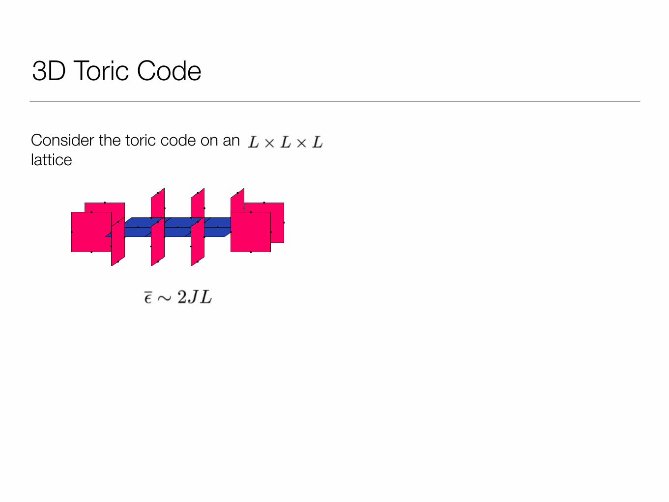
3D Toric Code
H = �JX
v
Av � JX
p
Bp
Consider the toric code on an lattice
3D Toric Code
Consider the toric code on an lattice

3D Toric Code
Consider the toric code on an lattice
leads to a bound

3D Toric Code
Consider the toric code on an lattice
leads to a bound
High temperature bound
Fernando Pastawski
Michael Kastoryano

Discussion of the bound
tmem ⇠ e�EB
• Relationship to Arrhenius law

Discussion of the bound
tmem ⇠ e�EB
• Relationship to Arrhenius law
• It would be nicer to have a bound that includes “entropic contributions”

Discussion of the bound
tmem ⇠ e�EB
• Relationship to Arrhenius law
• Can we get rid of the 1/N factor?
• It would be nicer to have a bound that includes “entropic contributions”

Proof sketch
• The Poincare Inequality
• Matrix pencils and the PI
• The canonical paths bound
• The spectral gap and the energy barrier

The Poincare Inequality
�Var�(f, f) E(f, f)
The Poincare Inequality
�⇣tr⇥�f†f
⇤� tr [�f ]2
⌘ �tr
⇥�f†L(f)
⇤
The Poincare Inequality
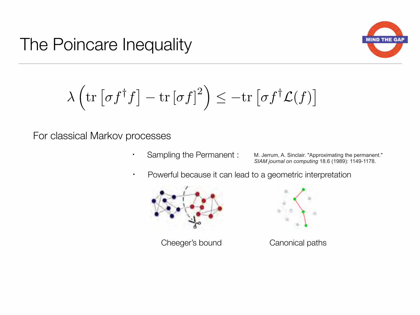
• Sampling the Permanent :
For classical Markov processes
Cheeger’s bound Canonical paths
M. Jerrum, A. Sinclair. "Approximating the permanent." SIAM journal on computing 18.6 (1989): 1149-1178.
• Powerful because it can lead to a geometric interpretation
�⇣tr⇥�f†f
⇤� tr [�f ]2
⌘ �tr
⇥�f†L(f)
⇤

The Poincare Inequality
• Sampling the Permanent :
For classical Markov processes
Challenges in the quantum setting
Cheeger’s bound Canonical paths
• We are missing a general geometric picture
M. Jerrum, A. Sinclair. "Approximating the permanent." SIAM journal on computing 18.6 (1989): 1149-1178.
• Powerful because it can lead to a geometric interpretation
�⇣tr⇥�f†f
⇤� tr [�f ]2
⌘ �tr
⇥�f†L(f)
⇤

Poincare and a Matrix pencil ��1 = ⌧
Var�(f, f) = (f |V|f)E(f, f) = (f |E |f)
⌧ E � V � 0⌧minimize subject to
�Var�(f, f) E(f, f)Equivalent formulation for
andwhere

Poincare and a Matrix pencil ��1 = ⌧
Var�(f, f) = (f |V|f)E(f, f) = (f |E |f)
⌧ E � V � 0⌧minimize subject to
�Var�(f, f) E(f, f)Equivalent formulation for
andwhere
AW = B⌧ = min kWk2
E = AA† V = BB†Lemma: Let
subject to
and
Boman, Erik G., and Bruce Hendrickson. "Support theory for preconditioning." SIAM Journal on Matrix Analysis and Applications 25.3 (2003): 694-717.

Suitable matrix factorization
L(f) ⇠X
i:↵i
(�↵ii f�↵i
i � f)� ! 0
E(f, f)
Some intuition from

Suitable matrix factorization
L(f) ⇠X
i:↵i
(�↵ii f�↵i
i � f)� ! 0
V(f) ⇠ 1
4N
X
�
(��11 . . .��N
N f��11 . . .��N
N � f)
E(f, f)
Var(f, f)
Some intuition from

Suitable matrix factorization
L(f) ⇠X
i:↵i
(�↵ii f�↵i
i � f)� ! 0
V(f) ⇠ 1
4N
X
�
(��11 . . .��N
N f��11 . . .��N
N � f)
E(f, f)
Var(f, f)
(�x
1f�x
1 � f) + (�z
2f�z
2 � f) + (�x
3f�x
3 � f) (�x
1�z
2�x
3 f �x
1�z
2�x
3 � f)
Choosing a decomposition in terms of
⇠
Some intuition from

Suitable matrix factorization
L(f) ⇠X
i:↵i
(�↵ii f�↵i
i � f)� ! 0
V(f) ⇠ 1
4N
X
�
(��11 . . .��N
N f��11 . . .��N
N � f)
E(f, f)
Var(f, f)
(�x
1�z
2�x
3 f �x
1�z
2�x
3 � f)(�x
1�z
2 f �x
1�z
2 � f) + (�x
3f�x
3 � f)
Choosing a decomposition in terms of
⇠
Some intuition from

Suitable matrix factorization
L(f) ⇠X
i:↵i
(�↵ii f�↵i
i � f)� ! 0
V(f) ⇠ 1
4N
X
�
(��11 . . .��N
N f��11 . . .��N
N � f)
E(f, f)
Var(f, f)
(�x
1�z
2�x
3 f �x
1�z
2�x
3 � f)(�x
1�z
2 f �x
1�z
2 � f) + (�x
3f�x
3 � f)
Choosing a decomposition in terms of
⇠
Some intuition from
A generalization yields to the matrix triple [A,B,W ]
kWk2 can be bounded by suitable norm bounds

Canonical paths bound
Dressed Pauli paths :
• The norm bound on can be evaluated in the following picture
kWk2

Canonical paths bound
Dressed Pauli paths :
• The norm bound on can be evaluated in the following picture
kWk2

Canonical paths bound
Dressed Pauli paths :
• The norm bound on can be evaluated in the following picture
kWk2

Canonical paths bound
⌧ max
⇠
4⌘⇤
2
Nh(!↵(b))⇢b
X
⌘a2�(⇠)
⇢a⇢a⌘
Dressed Pauli paths :
The matrix norm bound yields
• The norm bound on can be evaluated in the following picture
kWk2

The spectral gap and the energy barrier
• The only challenge is the maximum in the definition of ⌧

The spectral gap and the energy barrier
�⇠ : �(⇠) ! PN
Injective map (Jerrum & Sinclair)
• The only challenge is the maximum in the definition of ⌧

The spectral gap and the energy barrier
�⇠ : �(⇠) ! PN [�⇠(⌘a)]k =
⇢(0, 0)k : k ⇠⌘k : k > ⇠
Injective map (Jerrum & Sinclair)
• The only challenge is the maximum in the definition of ⌧

The spectral gap and the energy barrier
�⇠ : �(⇠) ! PN [�⇠(⌘a)]k =
⇢(0, 0)k : k ⇠⌘k : k > ⇠
Injective map (Jerrum & Sinclair)
Bounding ✏b⌘�⇠ + ✏b⇠ � ✏b � ✏b⌘ 2✏
⌧
• The only challenge is the maximum in the definition of ⌧

The spectral gap and the energy barrier
�⇠ : �(⇠) ! PN [�⇠(⌘a)]k =
⇢(0, 0)k : k ⇠⌘k : k > ⇠
Injective map (Jerrum & Sinclair)
Bounding h↵(!↵(a))⇢a⇢b�⇠(⌘b) � h⇤e��2✏⇢b⇢b⌘
⌧
• The only challenge is the maximum in the definition of ⌧

The spectral gap and the energy barrier
�⇠ : �(⇠) ! PN [�⇠(⌘a)]k =
⇢(0, 0)k : k ⇠⌘k : k > ⇠
Injective map (Jerrum & Sinclair)
Bounding h↵(!↵(a))⇢a⇢b�⇠(⌘b) � h⇤e��2✏⇢b⇢b⌘
⌧�0 4
⌘⇤
h⇤ e�2✏
max
⇠
X
⌘b2�(⇠)
1
2
N⇢b�⇠(⌘b)
⌧
• The only challenge is the maximum in the definition of ⌧

The spectral gap and the energy barrier
�⇠ : �(⇠) ! PN [�⇠(⌘a)]k =
⇢(0, 0)k : k ⇠⌘k : k > ⇠
Injective map (Jerrum & Sinclair)
Bounding h↵(!↵(a))⇢a⇢b�⇠(⌘b) � h⇤e��2✏⇢b⇢b⌘
⌧�0 4
⌘⇤
h⇤ e�2✏
max
⇠
X
⌘b2�(⇠)
1
2
N⇢b�⇠(⌘b)
| {z } 1
⌧
• The only challenge is the maximum in the definition of ⌧
Conclusion and Open Questions
• It would be great if one could extend the results to more general quantum memory models.
• This only provides a converse to the lifetime of the classical memory. It would be great if one could find a converse for the quantum memory time
• Can we get rid of the prefactor?
• Is it possible to find a bound that also takes the “entropic” contributions into account?