Thermal and Metallurgical Effects Associated with...

74 The Open Materials Science Journal, 2010, 4, 74-91

1874-088X/10 2010 Bentham Open

Open Access

Thermal and Metallurgical Effects Associated with Gas Carburized and Induction Hardened Components

K. Palaniradja*, N. Alagumurthi and V. Soundararajan

Department of Mechanical Engineering, Pondicherry Engineering College, Pondicherry – 605 014, India

Abstract: Dimensional distortion occurs due to the thermal and transformation stresses formed during the heat treatment

processes. Taguchi and Factorial design of experiment concepts were applied to optimize the operating variables involved

in the gas carburising and induction hardening processes so as to minimize the geometrical distortions. Experimental data

obtained for the materials EN353, EN351, AISI 4140, and AISI 9255 were analyzed by Response graph method and

Signal to Noise method. Even though, EN 351 and EN 353 are having the same carbon percentage, EN 353 gives minimal

dimensional and volume changes because of the presence of three alloying elements namely cobalt, molybdenum and

nickel. Analysis by variance (ANOVA) results indicated that the furnace temperature and quenching time in the gas

carburising process were the variables which had more influence on distortion. The percentage deviations between the

experimental and predicted results for the runout and helix variations were in the range of 7 to 10%.

Keywords: Thermal analysis, Metallurgical effects, surface hardness, helix variation, ANOVA.

1. INTRODUCTION

The major problem faced by heat treatment industries is the dimensional and geometrical changes that occur in the heat treated component. One of the main causes for dimensional changes is the stresses, which occur as a consequence of the contraction of the material during cooling, i.e. formation of thermal stresses (thermal effect). The other main cause is the transformation stresses which occur as a result of the marteniste formation (metallurgical effect).

When a body cools, the outer layer cools quicker and contracts first. The inner, softer parts try, during this process, to assume a spherical shape, this being the shape to which they offer the least resistance during deformation. Hence, the main rule is that all bodies with shape deviating from the spherical one attempt to assume this shape during cooling. Bullenes, D.K., (1949) illustrated that more the severity of the quench process greater will be the changes. Greater the rate of temperature drop during cooling greater will be the deformation [1].

On rapid heating and cooling of steel in any heat treatment process, it passes through a series of structural transformations. During heating of steels, a continuous increase in length occurs upto Ac1, where the steel starts shrinking as it transforms into austenite. After the austenite formation is completed, the length increases again. However, the coefficient of longitudinal expansion is not the same for austenite as that for ferrite.

On cooling, thermal contraction takes place and during martensite formation the length of the steel increases. After cooling to room temperature, most martensitic steels contain

*Address correspondence to this author at the Department of Mechanical Engineering, Pondicherry Engineering College, Pondicherry-605014, India; Tel: 91 413 2655281-287, Ext. 252,259; Fax: 91 413 2655101;

E-mail: [email protected]

some retained austenite, the amount increasing with the amount of alloying elements dissolved during austenitization. The larger the quantity of retained austenite contained in the steel after hardening the smaller is the increase in length or increase in volume. If the retained austenite content is sufficiently high, we generally obtain a reduction in volume [2].

Past experiences show that in surface hardening parts undergo volume and dimensional changes due to thermal fluctuations and phase transformations [3]. Dimensional changes can lead to excessive distortion in the components and results in excessive scrapage. Further, quench cracking can occur and the excessive grain growth in the region just below the hardened surface in the Gas carburizing and Induction hardening processes produces transformation stresses and thermal stresses (Thelning, 1984). These stresses cause shape and size distortion in the components. If the distortion is controlled within the tolerance limit, the post hardening processes can be eliminated by which cost and time can be saved. With this aim, experimental investigations have been carried out to study the thermal and metallurgical effects associated with Gas Carburizing and Induction hardening processes and the results are reported in this paper.

2. SHAPE AND SIZE DISTORTION IN GAS CARBURIZING

In case hardening process coping with deformation of materials is an important aspect. For long, considerable interest has been shown by researchers and practicing professionals to control if not totally overcome this problem. Normally, this problem of deformation is addressed by subjecting case hardened material to post-rectifying operations like straightening, machining, etc. [4].

The dimensional changes, which occur during case hardening, are governed by a wide variety of factors, as given below:

Thermal and Metallurgical Effects Associated with Gas Carburized The Open Materials Science Journal, 2010, Volume 4 75

The hardenability of the steel: More the hardenability and lesser the thickness of the material, more will be the volume increase.

Type of steel: It means the constituent alloying elements. The behaviour of Cr-Ni steels, Cr-Ni-Mo steels and to some extent Cr-Mn steels are similar in nature. On the other hand, Cr-Mo steels can exhibit some variations in behaviour as regards to change in shape.

Depth of case hardening: This factor is extremely difficult to assess because a considerable influence on the

structure, properties, and thickness of the case hardened layer is exercised both by the carbon content in the surface layer and by the hardening temperature. However, it is obvious that the depth of case hardening influences the dimensional changes.

Method of hardening: In principle, direct hardening causes the least dimensional variations and double hardening causes the greatest changes. The deformation increases with the number of heating and cooling cycles.

Table 1. Gas Carburizing Operating Conditions

S. No. Factors Notation Level 1 Level 2 Level 3

1 Furnace Temperature A 870°C 910°C 940°C

2 Quenching Time B 60 minutes 90 minutes 120 minutes

3 Tempering Temperature C 150°C 200°C 250°C

4 Tempering Time D 80 minutes 100 minutes 120 minutes

5 Preheating E No preheating 150°C No preheating

Table 2. Gas Carburizing Test Results Materials: EN353 and EN 351 – (Run-Out)

Run-Out in Microns

for EN 353

Run-Out in Microns

for EN 351

S/N

for Run-Out S. No. A B C D E

AQ AT AQ AT EN 353 EN 351

1 870 60 150 80 NO 70 70 110 110 23.098 19.172

2 870 60 200 100 150 40 40 60 72 27.958 23.573

3 870 60 250 120 NO 60 40 50 50 25.850 26.020

4 870 90 150 100 150 24 100 30 36 22.767 29.593

5 870 90 200 120 NO 24 90 50 54 23.627 25.673

6 870 90 250 80 NO 78 70 100 110 22.602 19.566

7 870 120 150 120 NO 102 80 120 105 20.756 18.957

8 870 120 200 80 NO 80 110 90 89 20.338 20.963

9 870 120 250 100 150 108 60 110 105 21.173 19.369

10 910 60 150 80 150 82 50 120 110 23.361 18.777

11 910 60 200 100 NO 28 30 60 65 30.746 24.075

12 910 60 250 120 NO 30 60 70 72 26.478 22.973

13 910 90 150 100 NO 60 100 40 44 21.674 27.525

14 910 90 200 120 NO 32 60 60 68 26.360 23.859

15 910 90 250 80 150 60 100 40 44 21.674 27.525

16 910 120 150 120 NO 50 90 60 67 22.757 23.931

17 910 120 200 80 150 62 45 100 98 25.324 20.086

18 910 120 250 100 NO 60 55 70 59 24.798 23.777

19 940 60 150 80 NO 20 40 40 36 30 28.392

20 940 60 200 100 NO 100 35 90 85 22.508 21.156

21 940 60 250 120 150 110 72 82 87 20.633 21.459

22 940 90 150 100 NO 32 24 40 44 30.969 27.525

23 940 90 200 120 150 22 20 25 36 33.545 30.175

24 940 90 250 80 NO 38 70 80 72 24.986 22.371

25 940 120 150 120 150 30 44 60 56 28.483 24.726

26 940 120 200 80 NO 30 44 40 47 28.483 27.202

27 940 120 250 100 NO 100 80 100 110 20.861 19.566

76 The Open Materials Science Journal, 2010, Volume 4 Palaniradja et al.

Material dimensions: A clear tendency towards shrinkage in the diameter of gears has been observed in connexion with small or moderate dimensional or material thicknesses. As the dimensions of gears and rings increase, the shrinkage decreases, and at a certain dimension there is an increase in the diameter.

The main problem in the Gas carburized components is shape and size distortion. Shape distortion can be reduced by proper stress relieving between machining as they are mostly due to residual stresses. Whereas, size distortion is due to structural transformations in steel. When austenite transforms into martensite there is an expansion in volume. While tempering there is a contraction due to the formation of carbides. The presence of retained austenite and its change during tempering introduces complex overall changes in

size. Many literatures indicate that the following are some of the reasons for distortion.

Due to rapid heating

Methods of stacking or fixturing of parts

Increase in grain growth with increase in case depth

Severity of quenching

One of the objectives of the present work is to minimizing the distortion level (in the present case, run-out and helix-variations) in pinion made of EN 353 and EN 351 material (used in power steering assembly) with optimum case depth and surface hardness value. Taguchi’s mixed level series [5]. Design of Experiment is adopted to arrive at the level of process parameters, which will minimize the distortion in heat treated material [6].

Table 3. Gas Carburizing Test Results Materials: EN353 and EN 351 (Helix Variations – Left)

Left – Helix Variations in Microns

EN 353 EN 351

S/N

for Helix-Variation (Left) S. No. A B C D E

BHT AHT BHT AHT EN 353 EN 351

1 870 60 150 80 NO 13.2 40.2 40.2 17.5 30.481 30.172

2 870 60 200 100 150 13.2 15.2 15.6 16.2 36.932 35.970

3 870 60 250 120 NO 70.2 48.2 60.1 62.2 24.406 24.270

4 870 90 150 100 150 0.7 52.6 52.3 0.7 28.589 28.639

5 870 90 200 120 NO 13.2 12.4 12.4 12 37.851 38.271

6 870 90 250 80 NO 13.2 38.4 37.8 15.2 30.838 30.809

7 870 120 150 120 NO 40 30.4 30.2 46.0 28.989 28.198

8 870 120 200 80 NO 7.2 24.2 28.4 7.2 34.965 33.673

9 870 120 250 100 150 24.1 22.1 19.1 28.2 32.719 32.365

10 910 60 150 80 150 44.4 1.5 7.9 44.0 30.057 30.003

11 910 60 200 100 NO 4.2 72 82 6.0 25.848 24.710

12 910 60 250 120 NO 46 0 2.4 44 29.755 30.128

13 910 90 150 100 NO 11.8 12.5 14.6 12.4 38.304 37.364

14 910 90 200 120 NO 44.2 34.6 40 48.4 28.026 27.052

15 910 90 250 80 150 13.1 36.7 36.7 16.2 31.196 30.943

16 910 120 150 120 NO 27 36 37.2 29.3 29.946 29.503

17 910 120 200 80 150 0.9 42.5 42.3 1.2 30.440 30.48

18 910 120 250 100 NO 42.7 35.5 37.7 40 28.119 28.208

19 940 60 150 80 NO 14.6 33.2 34.8 14.7 31.819 31.465

20 940 60 200 100 NO 24.8 48.2 49.2 28.2 28.329 27.937

21 940 60 250 120 150 46 17.1 10.2 18.3 29.193 36.586

22 940 90 150 100 NO 44 32.2 34.2 44.2 28.278 28.064

23 940 90 200 120 150 2.8 0.7 1.4 4.5 53.803 49.544

24 940 90 250 80 NO 54.4 24.2 27.2 56.2 27.514 27.101

25 940 120 150 120 150 0.82 22.5 27.2 1.9 35.960 34.297

26 940 120 200 80 NO 40.1 50 56 36.2 26.873 26.530

27 940 120 250 100 NO 1.8 15.6 17.4 1.9 39.090 38.147


The significance in this study is the three stages of carburizing (Pre carburizing, Carburizing and Post carburizing) are considered for optimization [7]. An orthogonal array and ANOVA are employed to investigate the influence of major process variables on Distortion level, Surface hardness and Case depth. Optimum conditions have been arrived at by applying high penetration depth, high hardness and low distortions are better as the strategies. Response graph and Signal to Noise ratio methods are followed to predict the optimum results and the results are compared.

The conditions underwhich the gas carburizing experiments have been carried out are given in Table 1. The run-out of the pinion after quenching (AQ) and after tempering (AT) of the pinion materials are measured using

mechanical dial gauge. The left and right helix variations before heat treatment (BHT) and after heat treatment (AHT) of the pinion materials are measured using a gear tester. The measured values are tabulated in Tables 2-4.

The experiments have been conducted based on L27 orthogonal array system proposed in Taguchis’ Mixed Level Series of DOE with interactions as given below:

i) Furnace Temperature vs Quenching Time (AxB)

ii) Furnace Temperature vs Tempering Temperature (AxC)

2.1. Response Graph Method

Response graphs are shown in Figs. (1a-e, 2a-e) drawn using the values in Tables 5-7.

Table 4. Gas Carburizing Test Results Materials: EN353 and EN 351 – (Helix Variations – Right)

Right – Helix Variations in Microns

EN 353 EN 351

S/N

for Helix-Variation (Right) S. No. A B C D E

BHT AHT BHT AHT EN 353 EN 351

1 870 60 150 80 NO 45.2 50.15 69.4 43.5 26.422 24.743

2 870 60 200 100 150 58.2 48.2 71.4 44.3 25.443 24.521

3 870 60 250 120 NO 68.4 112.4 67.2 110.2 20.626 20.793

4 870 90 150 100 150 26.8 60 24.4 62 26.657 26.537

5 870 90 200 120 NO 46.2 4.2 44.4 5.5 29.681 29.996

6 870 90 250 80 NO 29.4 82 29.3 80.2 24.208 24.382

7 870 120 150 120 NO 104.3 44 105.4 42.2 21.933 21.907

8 870 120 200 80 NO 34.2 25.2 34.5 24.4 30.446 30.492

9 870 120 250 100 150 8.1 72.4 9.2 72.3 25.761 25.757

10 910 60 150 80 150 65.2 50.1 72.1 50.3 24.710 24.129

11 910 60 200 100 NO 46.2 89.2 48.2 85.4 22.970 23.180

12 910 60 250 120 NO 38.41 2.1 39.2 0.5 31.308 31.143

13 910 90 150 100 NO 34.3 24.4 37.2 20.4 30.526 30.457

14 910 90 200 120 NO 42 40.8 41 41.4 27.659 27.701

15 910 90 250 80 150 32.2 42.4 32.2 46.1 28.485 28.010

16 910 120 150 120 NO 52.4 32.4 54.2 37.2 27.217 26.653

17 910 120 200 80 150 17.6 51.2 17.2 54.4 28.339 27.884

18 910 120 250 100 NO 39.2 24.5 40.1 24.4 29.712 29.579

19 940 60 150 80 NO 28.4 23.5 29.4 28.4 31.678 30.780

20 940 60 200 100 NO 38.2 31.5 37.2 34.6 29.116 28.892

21 940 60 250 120 150 10.2 32.4 12.4 31.3 32.388 32.466

22 940 90 150 100 NO 26.2 44.5 27.2 44.4 28.750 28.678

23 940 90 200 120 150 0.9 20.4 0.5 20.4 36.809 36.815

24 940 90 250 80 NO 54.2 40.2 54.6 52 26.426 25.462

25 940 120 150 120 150 6.2 35.4 7.2 35.4 31.899 31.854

26 940 120 200 80 NO 42.4 58.2 42.1 58.6 25.862 25.844

27 940 120 250 100 NO 21.2 6.3 20.4 4.8 36.116 36.583


2.1.1. Influence of Main Variables on Run-Out

ANOVA analysis is carried out to determine the influence of main variables on run-out and also to determine the percentage contributions of each factor. Table 8 shows the results of percentage contribution of each variable for run-out.

2.1.1.1. Model Calculation for EN 351

Correction factor, C.F,

= [

yi ]2 / Number of Experiment

= [110+66+…..105]2 /27

=119533.77

Total sum of squares, SST

=

yi 2 – C.F

=129254-119533.77

= 9720.23

Sum of Squares of Factors, Variable A, SSA

= [

y12 /9+

y2

2 /9+

y3 2/9] –

C.F

= [51604.09+36992.11+32160.44]-C.F

= 120757.25-119533.77

= 1223.48

Percentage contribution of each factor, A = (SSA/SST)*100

= (1223.48 /9720.2) *100

=12.58%

In the same way the percentage contribution of other variables are calculated.

Table 5. Average Effect of Process Variables on Run-Out

Level 1

Run-Out

Level 2

Run-Out

Level 3

Run-Out Variables

EN 353 EN 351 EN 353 EN 351 EN 353 EN 351

Furnace temperature 72.111 80.611 58.56 69.28 50.6111 61.9444

Quenching Time 57.167 65.056 55.778 54.056 67.11 82.56

Tempering Temperature 59.33 68.22 49.56 66.06 69.5 78.39

Tempering Time 62.17 68.78 59.78 67.78 56.44 65.11

Preheating 65.06 81.94 59.39 70.61 - -

Table 6. Average Effect of Process Variables on Left -Helix Variations

Level 1

Left - Helix

Level 2

Left - Helix

Level 3

Left - Helix Variables

EN 353 EN 351 EN 353 EN 351 EN 353 EN 351


Quenching Time 30.68 30.75 24.5389 25.9111 25.746 27.078


Tempering Time 27.4 28.8722 26.289 27.772 27.34 27.0944

Preheating 27.267 29.039 19.829 19.106 - -

Table 7. Average Effect of Process Variables on Right -Helix Variations

Level 1

Right - Helix

Level 2

Right - Helix

Level 3

Right - Helix Variables

EN 353 EN 351 EN 353 EN 351 EN 353 EN 351


Quenching Time 46.99778 48.61111 36.17222 37.95556 37.5111 38


Tempering Time 42.875 45.48333 38.85555 39.32777 38.50611 38.64444

Preheating 35.67556 36.85556 35.43889 36.83889 - -


Total contribution of factors = (A+B+C+D+AxB+AxC)

= 88.19%

Error = 11.81%

(a)

(b)

(Fig. 1) contd…..

(c)

(d)

45

50

55

60

65

70

75

80

85

860 870 880 890 900 910 920 930 940 950

Furnace temperature in degree Celsius

EN 353 EN 351

Ave

rage

val

ue

of R

un

-ou

t in

mic

ron

s

45

50

55

60

65

70

75

80

85

0 20 40 60 80 100

Quenching time in minutes

EN 353 EN 351

Ave

rage

val

ue

of R

un

-ou

t in

mic

ron

s

45

50

55

60

65

70

75

80

85

0 50 100 150 200 250 300

Tempering temperature in degree Celsius

EN 353 EN 351

Ave

rage

val

ue

of R

un

-ou

t in

mic

ron

s

55

57

59

61

63

65

67

69

71

0 20 40 60 80 100 120 140

Tempering time in minutes

EN 353 EN 351

Ave

rage

val

ue

of R

un

-ou

t in

mic

ron

s


(Fig. 1) contd…..

(e)

Fig. (1). (a-e) Process variables vs run-out.

Table 8. Percentage Contribution of Each Variable on Run-

Out

Run-Out Variables

EN 353 EN 351

Furnace temperature 14.53% 12.58%

Quenching Time 12.82% 11.84%

Tempering Temperature 6.12% 5.19%

Tempering Time 7.94% 7.98%

Preheating 14.19% 15.88%

Furnace Temperature and Quenching time 26.43% 27.58%

Furnace Temperature and Tempering Temperature 5.98% 7.14%

Error 11.99% 11.81%

Optimum set of variables for run-out is found by adopting the Lower is better strategy. The results are given in Table 9.

2.2. Prediction of Mean Response (Run-Out)

From Taguchis’ methodology, equation (1) can be used to predict the run-out obtainable.

= T+ (RAopt –T) + (RBopt –T) + (RCopt - T) + (RDopt - T) + (REopt - T) (1)

where,

-predicted mean response.

T-mean of all observed run-out values;

RA opt, RB opt, RC opt, RD opt, and RE opt – Runout values obtained at optimum process variable conditions.

Table 9. Optimum Conditions for Run-Out for EN 353 and

EN 351

Run-Out Variables

EN 353 EN 351

Furnace temperature 940°C 940°C

Quenching Time 90 minutes 90 minutes

Tempering Temperature 200°C 200°C

Tempering Time 120 minutes 120 minutes

Preheating 150°C 150°C

2.2.1. Model Calculation for EN 353 Material

T={(110+66+50+33+52+105+112.5+89.5+107.5+115+62.5+71+42+64+42+63.5+99+64.5+38+87.5+84.5+42+30.5+76+58+43.5+105)/27} (Table 2)

T = 70.888

RAopt= 61.94

RBopt= 54.056 from Table 5

RCopt= 66.06

RD opt= 65.11

RE opt= 70.61

(Run-out) = 70.888+ (61.94 –70.888) + (54.056 –70.888) + (66.06 –70.888) + (65.11 –70.888) + (70.61–70.888) = 34.224 microns.

Similarly, for EN 353 the predicted mean response, = 33.998 microns.

Optimum Run-out value, for EN 353 - 33.998 microns and EN 351 – 34.224 microns.

2.2.1.1. Influence of Main Variables on Helix-Variations

ANOVA analysis is carried out to determine the influence of main variables on helix variations (left) and also to determine the percentage contribution of each variable. Table 10 shows the results of percentage contribution of each factor for helix-variation (Left).

Model Calculation for EN 353

Correction factor, C.F

= [

yi ]2 / Number of Experiment

= [26.7+14.2+…..8.7]2 /27

=19664.64

Total sum of squares, SST

=

yi2 – C.F

=23936.44-19664.64

= 4271.8

55

60

65

70

75

80

85

0 20 40 60 80 100 120 140 160

Preheating temperature in degree Celsius

EN 353 EN 351

Ave

rage

val

ue

of R

un

-ou

t in

mic

ron

s


Sum of Squares of Factors,

Variable, A SSA

= [

y12 /9+

y2

2 /9+

y3 2/9] –

C.F

= [6365.38+7100.87+6342.20]-C.F

= 19808.45-19664.64

= 143.81

Percentage contribution of each factor, A = (SSA/SST)*100

= (143.81/4271.8) *100

=3.36%

In the same way the percentage contribution of other variables are calculated.

Total contribution of factors = (A+B+C+D+E+AxB+AxC) = 82.43%

Error =17.6%

Table 10. Percentage Contribution of Each Variable on Helix

Variation (Left)

Helix Variation

(Left) Variables

EN 353 EN 351








Error 17.6% 15.11%

Optimum set of variables for helix-variations (left) are found by adopting the Lower is better strategy. The results are given in Table 9.

2.2.2. Prediction of Mean Response (Helix Variations-Left)

From Taguchis’ methodology, equation (2) can be used to predict the Helix variations (Left) obtainable,

= T+ (LAopt –T) + (LBopt –T) + (LCopt - T) + (LDopt - T) + (LEopt - T) (2)

where,

-predicted mean response

T-mean of all observed Helix- variations (Left) values; LA opt, LB opt, LC opt, LD opt, and LE opt - helix variations (Left) values obtained at optimum process variable condition.

2.2.2.1. Model Calculation for EN 353 Material

T = {(26.7+14.2+59.2+26.65+12.8+25.8+35.2+15.7+23.1+ 22.95+38.1+23+12.15+39.4+24.9+31.5+21.7+39.1+23.9+36.5+31.55+38.1+1.75+39.3+11.66+45.05+8.7)/27} (from Table 3)

T = 26.98

LAopt= 25.279

LBopt= 24.5389

LCopt= 25.022 (From Table 6)

LD opt= 27.34

LE opt= 19.829

(helix variations -left) = 26.98+ (25.279 –26.98) + (24.5389 –26.98) + (25.022 –26.98) + (27.34–26.98) + (27.34–26.98) = 21.5999 microns

Similarly for EN 353 the predicted mean response = 21.5999 microns.

Predicted mean difference is given by, EN 353 – 21.5999 microns and EN 351 – 13.790 microns.

(a)

20

25

30

35

40

45

50

55

860 880 900 920 940 960 Furnace temperature in degree Celsius

Ave

rage

val

ue o

f he

lix

- va

riat

ions

in m

icro

ns

EN 353 - Left Helix EN 351 - Left Helix

EN 353 - Right Helix EN 351 - Right Helix


(Fig. 2) contd….. (Fig. 2) contd…..

Fig. (2). (a-e) Process variables vs Helix variations (Left and

Right).

20

25

30

35

40

45

50

0 50 100 150 200 250 300 Tempering temperature in degree Celsius

(c)

Ave

rage

val

ue o

f he

lix

vari

atio

ns in

mic

rons

EN 353 - Helix Left EN 351 - Helix Left

EN 353 - Helix Right EN 351 - Helix Right

20

25

30

35

40

45

50

55

0 20 40 60 80 100

Quenching time in minutes(b)

Ave

rage

val

ue o

f he

lix-

vari

atio

ns

in m

icro

ns

EN 353 - Helix left EN 351 - Helix Left


20

25

30

35

40

45

50

0 20 40 60 80 100 120 140 Tempering time in minutes

(d)

Ave

rage

val

ue o

f he

lix-

vari

atio

ns

in m

icro

ns



15

20

25

30

35

40

0 50 100 150 200 Preheating Temperature in degree Celsius

(e)



Ave

rage

val

ue

of h

elix

var

iati

ons

in m

icro

ns


Similarly, the percentage contributions of each variable on the helix variation- (Right) is calculated and given in the Table 11.

Table 11. Percentage Contribution of Each Variable on Helix

Variations (Right)

Helix Variation

(Right) Variables

EN 353 EN 351








Error 8.56% 9.98%

Optimum set of variables for helix variations (Right) are found by adopting the Lower is better strategy [8]. The results are given in Table 9. Predicted mean difference for helix variation (right) is calculated and given below.

EN 353 – 17.77 microns and EN 351 – 19.03 microns.

Signal to Noise Ratio

Formula to determine S/N ratio for minimizing the response factor as the objective (Minimizing the run-out and helix variations) is, [9-10].

S/N = -10 Log10 [ yi2 / n] (3)

where, yi - is the experimental response values for the trials, n - number of trials

S/N ratio for run-out and helix variations (Left and Right) are calucated using the equation 3. The model calculation is given below and the S/N ratios for run-out, Helix variation (Left) and Helix variation (right) are listed in the Tables 2-4 respectively.

2.2.2.2. Model Calculation for the Material EN 353 – Run-Out

S/N ratio for minimizing the run-out (12th Experiment run)

S/N = - 10 log10 [{(0.03)2 +(0.06)2}/2]

= 26.478

Similarly for EN 351 steel material – Helix variation –Left

S/N ratio for minimizing the variation in helix -left (16th Experiment run)

S/N = - 10 log10 [{(0.0423)2 + (0.0012)2}/2]

= 30.48

Similarly, for EN 353 steel material – Helix variation –Right

S/N ratio for minimizing the variation in helix -left (08th Experiment run)

S/N = - 10 log10 [{(0.0342)2 + (0.0252)2}/2]

= 30.4463

Optimum conditions for run-out and helix variations are found by adopting the higher the S/N ratio is better as the strategy and results are given in the Table 9 for the materials EN 353 and EN 351. The optimum conditions result obtained in S/N method matches with the optimum result obtained from the response graph analysis. It is significant to note that the optimum conditions for hardness, case depth, run out and helix variations are the same (Tables 7 and 9 in Paper 1).

3. VOLUME AND DIMENSIONAL CHANGES IN INDUCTION HARDENING

Induction hardening processes have been well developed and widely used in the various industrial applications especially in treating automobile transmission gears for several decades. However, due to the complex geometry of gears and the volume changes involved in the hardening process, it is very difficult to surface harden the gears with the required degree of consistency and quality. Minimization of changes in volume and accompanying dimensional changes arising from the high temperature heat treatment processes have been the critical issues.

The demerits involved in induction hardening are,

Volume changes and dimensional changes which may require reworking

Quench cracking

Excessive grain growth in the region just below the hardened surface in the Induction hardening process produces transformation stresses and thermal stresses. These stresses cause shape and size distortion in the components. The term ‘distortion’ usually describes the dimensional changes brought about by the relief of internal stresses, which occur in a component after heat treatment.

Several investigations have found it convenient to divide the total distortion into two classes of dimensional change. The first of these is usually called ‘volume change’ or ‘inherent distortion’ and is said to be the result of the dilations due to transformations. The second type of dimensional change is usually ‘warpage’ or ‘change in shape’ and is said to be associated with the thermal stresses produced by non-uniformity of heating or cooling. In this investigation, the term ‘distortion’ refers to the total dimensional change that has resulted from a particular heat-treatment operation, namely Induction hardening [11].

The distortion has always presented difficulties to users of the many varieties of steels, which can be hardened by Induction hardening [12]. The dimensional change in Induction hardened components is troublesome to manufacturers. If the distortion is controlled within the tolerance limit, the post hardening processes can be eliminated by which cost and time can be saved [13]. With this aim, a study has been conducted in this present work to minimize the distortion level in the sample material (i.e. Rack made of AISI 4140 and AISI 9255).

The details of materials and operating conditions used in the experiments are shown in Table 12.


Table 13 shows the experimental results in the 33 Design Matrix for the materials AISI 4140 and AISI 9255 respectively.

Tables 14 and 15 show the ANOVA with F-Test for the materials AISI 4140 and AISI 9255 respectively.

The experiments have been conducted based on 33 full factorial DOE.

3.1. Influence of Main Variables on Distortion of Rack Material

3.1.1. Model Calculation

Total sum of the run = (2.4+2.3+2.5+……….0.9+1.0+0.8) = 128.4

Table 12. Materials and Operating Conditions

Levels Actual Code S. No. Variables Unit Notation

Low Medium High Low Medium High

1 Power potential kW/inch2 P 5.5 7.05 8.5 L1 L2 L3

2 Scan speed m/min S 1.34 1.72 2.14 L1 L2 L3

3 Quench flow rate Litres/min Q 15 17.5 20 L1 L2 L3

Table 13. 33 Design Matrix for Induction Hardening with Test Results

AISI 4140

Distortion in mm

AISI 9255

Distortion in mm S. No. P S Q

Trial 1 Trial 2 Trial 3 Trial 1 Trial 2 Trial 3

1 5.5 1.34 15 2.3 2.2 2.4 2.4 2.3 2.5

2 5.5 1.34 17.5 2 1.9 2.1 2.4 2.3 2.2

3 5.5 1.34 20 2.1 2.1 2.1 2.2 2.4 2.3

4 5.5 1.72 15 1.3 1.2 1.1 1.9 2.1 2.0

5 5.5 1.72 17.5 2.3 2.1 2.2 2.1 2.2 2.1

6 5.5 1.72 20 1.5 1.4 1.3 1.4 1.6 1.5

7 5.5 2.14 15 2.3 2.3 2.3 1.7 1.8 1.6

8 5.5 2.14 17.5 2.2 2.1 2.3 2.3 2.2 2.1

9 5.5 2.14 20 2 1.9 2.1 1.9 2 2.1

10 7.05 1.34 15 2.1 2.1 2.1 1.6 1.7 1.8

11 7.05 1.34 17.5 1.6 1.6 1.8 1.7 1.7 2

12 7.05 1.34 20 1.3 1.2 1.4 1.9 1.8 2

13 7.05 1.72 15 1.5 1.6 1.7 1.3 1.5 1.4

14 7.05 1.72 17.5 1.2 1.2 1.2 1.4 1.5 1.6

15 7.05 1.72 20 1.9 2 2.1 1.7 2 1.7

16 7.05 2.14 15 2 2.2 2.1 1.9 1.8 2

17 7.05 2.14 17.5 1.5 1.3 1.4 1.7 1.7 2

18 7.05 2.14 20 1 1.1 0.9 1.2 1.3 1.4

19 8.5 1.34 15 0.8 0.7 0.9 1.5 1.3 1.4

20 8.5 1.34 17.5 2 1.9 2.1 1 0.8 0.9

21 8.5 1.34 20 1 0.9 1.1 1.2 1.2 1.2

22 8.5 1.72 15 0.8 0.8 0.5 1.1 1 0.9

23 8.5 1.72 17.5 1.1 1.1 1.1 1 1 1

24 8.5 1.72 20 1 0.8 0.9 1 1.2 1.1

25 8.5 2.14 15 1.2 1.2 1.2 0.8 1 0.9

26 8.5 2.14 17.5 0.9 0.9 0.9 0.7 0.9 0.8

27 8.5 2.14 20 0.9 0.7 0.8 0.9 1 0.8


Number of Treatments = 3 (3 Factors)

Number of Levels = 3

Number of replicates (r) = 3

Total of the observations under all factor levels, =N= abcr = 3x3x3x3=81

Correction factor, (C) = (128.4)2/81 =203.5

Sum of Squares of Treatment, (SST) = (2.42 +2.32+2.52+ …0.92+12+0.82)

= 223.04 - C =19.54

Sum of Squares of Treatment with replicates, (SSTr) = 1/3(7.22+ 6.92+…2.72)

= 1/3(667.3)-C =18.93

Sum of Squares of Replicate, (SSR) = 1/27(41.82+43.32+43.32)-C = 0.093

Sum of Squares of Error, (SSE) = SST-SSTr – SSR = 19.54-18.93-0.093 =0.517

S Q Q

55.5 21 16.8 17.7 47.7 16.5 15 16.2

45.3 16.2 14.1 15 40.2 13.5 13.5 13.2

27.6 10.5 9.3 7.8

P

40.5 13.5 14.4 12.6

128.4 47.7 40.2 40.5 55.5 18.6 19.5 17.4 128.4 43.5 42.9 42

45.3 15 15.3 15

27.6 9.9 8.1 9.6

128.4 43.5 42.9 42 P

S

3.1.2. Sum of Squares of Main Effect (P, S and Q)

Sum of Square of Power Potential, SSP = [1/27(55.52+45.32+27.62)]-C = 14.8

Sum of Square of Scan Speed, SSS = [1/27(47.72+40.22+40.52)]-C = 1.373

Sum of Square of Quench flow rate, SSQ = [1/27(43.52+42.92+422)]-C = 0.08

3.1.3. Two Way Interactions of Sum of Squares (PS, SQ and PQ)

Sum of Square of Power Potential and Scan Speed = [1/9(212+…7.82)] –C = 0.367

Sum of Square of Scan Speed and Quench flow rate = [1/9(16.52+….12.62)]-C = 0.247

Sum of Square of Power Potential and Quench flow rate = [1/9(18.62+…9.62)]-C = 0.380

3.1.4. Three Way Interactions of Sum of Square (PSQ)

Sum of Square of Power Potential, Scan speed and Quench flow rate = SSTr - {SSP-SSS-SSQ-SSPS- SSSQ-SSPQ}

= 18.93-14.8-1.373-0.08-0.367-0.247-0.38 =1.683

Regression analysis has been done using MATLAB and the Regression equations (Equation to predict the distortion of the material AISI 4140) have been arrived at. The results are given below.

AISI 4140

Coeff =

1.0000 5.5000 1.3400 15.0000 2.3

1.0000 5.5000 1.3400 17.5000 2.0

1.0000 5.5000 1.3400 20.0000 2.1

1.0000 5.5000 1.7200 15.0000 1.2

1.0000 5.5000 1.7200 17.5000 2.3

Table 14. ANOVA with F-Test - Material: AISI 4140

Variable Sum of Squares Degrees of Freedom Mean Square F Significant Ranking

Replicates 0.0574 2 0.0287 3.776 -

P 5.549 2 2.7745 365.065 1

S 5.1935 2 2.5965 341.644 2

Q 1.00976 2 0.50488 66.431 6

PS 4.678 4 1.1695 153.881 3

SQ 3.82124 4 0.95531 125.698 4

PQ 2.07124 4 0.51781 68.132 5

PSQ 0.69446 8 0.0868 11.421 7

ERROR 0.3959 52 0.0076 -

TOTAL - 80


1.0000 5.5000 1.7200 20.0000 1.4

1.0000 5.5000 2.1400 15.0000 2.3

1.0000 5.5000 2.1400 17.5000 2.2

1.0000 5.5000 2.1400 20.0000 2.0

1.0000 7.0500 1.3400 15.0000 2.1

1.0000 7.0500 1.3400 17.5000 1.6

1.0000 7.0500 1.3400 20.0000 1.3

1.0000 7.0500 1.7200 15.0000 1.6

1.0000 7.0500 1.7200 17.5000 1.3

1.0000 7.0500 1.7200 20.0000 2.0

1.0000 7.0500 2.1400 15.0000 2.1

1.0000 7.0500 2.1400 17.5000 1.4

1.0000 7.0500 2.1400 20.0000 1.0

1.0000 8.5000 1.3400 15.0000 0.8

1.0000 8.5000 1.3400 17.5000 2.0

1.0000 8.5000 1.3400 20.0000 1.0

1.0000 8.5000 1.7200 15.0000 0.7

1.0000 8.5000 1.7200 17.5000 1.1

1.0000 8.5000 1.7200 20.0000 1.0

1.0000 8.5000 2.1400 15.0000 1.3

1.0000 8.5000 2.1400 17.5000 0.9

1.0000 8.5000 2.1400 20.0000 0.8

The coefficients for the formation of distortion equation are,

4.7850

-0.1993

-0.3480

-0.0711

Equation to predict the distortion of the material AISI 4140,

YD = 4.7850-0.1993P-0.3480S-0.0711Q (4 )

Similarly for the material AISI 9255,

YD = 4.6698-0.3415P-0.3195S-0.0078Q (5)

4. RESULTS AND DISCUSSION

4.1. Surface Hardening- Gas Carburizing

The pinion material surface is case hardened by Gas carburizing heat treatment process. For the desired application, the case depth required is between 0.8 – 1.00mm and the hardness between 79-82 HRA.

Distortion, is the major defect faced in gas carburizing process. Distortion here refers to Run-out and unwinding of helix angle in pinion [14]. To minimize the distortion level in pinion and to analyze the experimental data by Response graph method and Signal to Noise method the values of Run-out and helix variations (Left and Right) are checked for the materials EN353 and EN351.

Average effect of the main variables on Run-out, Left and Right helix variations for the materials EN353 and EN351 are shown in the Tables 5-7. Corresponding Response graphs, Figs. (1a-e, 2a-e) are drawn.

Even though, EN 351 and EN 353 are having same carbon percentage, EN 353 gives minimal dimensional and volume changes because of the presence of three alloying elements namely Cobalt, Molybdenum and Nickel. These steels have properties which are superior to corresponding double alloy steels ie. (Nickel and Chromium) alloy steels. Under optimum conditions, the distortions for the above said materials are given in the Table 16 below (taken from Tables 2-4) and it validates the above said statement.

Table 16. Distortion Level Under Optimal Conditions

Materials: EN 351 and EN 353

Helix Variations in Microns S. No. Materials

Run-Out

in Microns Left Right

01 EN 351 36 4.5 20.4

02 EN 353 21 0.7 20.4

Table 15. ANOVA with F-Test - Material: AISI 9255

Variable Sum of Squares Degrees of Freedom Mean Square F Significant Ranking

Replicates 0.093 2 0.0465 4.696 -

P 14.8 2 7.4 747.474 1

S 1.373 2 0.6865 69.343 2

Q 0.08 2 0.04 4.040 7

PS 0.367 4 0.09175 9.267 5

SQ 0.247 4 0.06175 6.237 6

PQ 0.380 4 0.095 9.595 4

PSQ 1.683 8 0.210 21.212 3

ERROR 0.517 52 0.0099 -

TOTAL - 80


(a)

(b)

(Fig. 3) contd…..

(c)

Fig. (3). (a-c) Process variables vs Distortion.

Analysis of variance is done for EN 353 and EN 351. The ANOVA results (Tables 8, 10 and 12) and optimum conditions (Tables 9, 11 and 13) indicate that the interaction between Furnace temperature and quenching time is having more influence on the distortion. Confirmation trail for optimum condition is carried out and results are tabulated in Table 17 and it shows that a good agreement between the experimental results and predicted optimum results. The percentage deviation between the experimental and predicted results for the runout and helix variations is in the range of 7 to 10%.

Similarly, Signal to noise ratio method has also given the same optimal variable levels/best treatment combination levels for the materials EN353 and EN 351 (Table 4).

At present, straightening operation is required to remove the bend in a 5 tons Hydraulic press as it occurs during the heat treatment process. Straightening operation incurs additional manpower and cost of manufacturing. This may be clear from the following cost analysis.

Pinion manufacturing cost : Rs. 80/-

Re-working cost : Rs. 8/-

Average number of pinion produced per annum : 75,000 nos.

Average percentage of rejection of pinion : 10% (7,500 nos.)

1

1.2

1.4

1.6

1.8

2

2.2

0 2 4 6 8 10

Power potential in kW/sq.inch

Ave

rage

dis

tort

ion

val

ue

in m

m AISI 4140 AISI 9255

1

1.1

1.2

1.3

1.4

1.5

1.6

1.7

1.8

1.9

0 0.5 1 1.5 2 2.5

Scan speed in m/minutes

AISI 4140 AISI 9255

(b)

A

vera

ge d

isto

rtio

n v

alu

e in

mm

1.3

1.35

1.4

1.45

1.5

1.55

1.6

1.65

1.7

1.75

1.8

0 5 10 15 20 25

Quench flow rate in litres /min

Ave

rage

dis

tort

ion

val

ue

in m

m

AISI 4140 AISI 9255

(c)


Cost of rejection per annum : 7500*88*12

: Rs.7.2 lakhs (approx.)

: $US 15,000/- (approx.)

Hence, introduction of optimum conditions gives great economical benefits and increases the rate of production [15].

In Gas carburization, by eliminating the final straightening operation cost saved per year is Rs.7.0 Lacs. (US$ 15,000) and the time saved per loading is 6 hours.

The present study shows that under optimum conditions the pinion product obtained do not require any re-working process. This is due to the fact that under optimum treatment combination, the Run-out in pinion is within 30 microns and unwind of helix angle is within 40 microns, which are well within the maximum permissible limits [16].

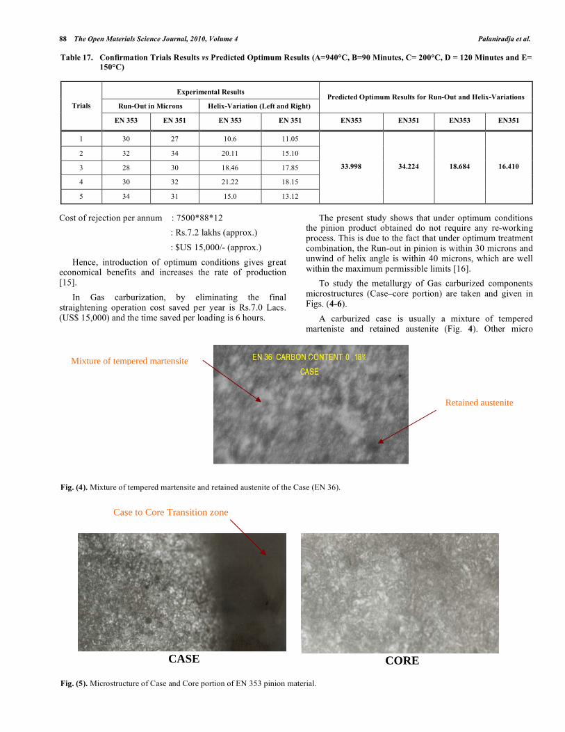
To study the metallurgy of Gas carburized components microstructures (Case–core portion) are taken and given in Figs. (4-6).

A carburized case is usually a mixture of tempered marteniste and retained austenite (Fig. 4). Other micro

Table 17. Confirmation Trials Results vs Predicted Optimum Results (A=940°C, B=90 Minutes, C= 200°C, D = 120 Minutes and E=

150°C)

Experimental Results

Run-Out in Microns Helix-Variation (Left and Right)

Predicted Optimum Results for Run-Out and Helix-Variations

Trials

EN 353 EN 351 EN 353 EN 351 EN353 EN351 EN353 EN351

1 30 27 10.6 11.05

2 32 34 20.11 15.10

3 28 30 18.46 17.85

4 30 32 21.22 18.15

5 34 31 15.0 13.12

33.998 34.224 18.684 16.410

Fig. (4). Mixture of tempered martensite and retained austenite of the Case (EN 36).

Fig. (5). Microstructure of Case and Core portion of EN 353 pinion material.

CASE

CORE

Case to Core Transition zone

Mixture of tempered martensite

Retained austenite


constituents, such as primary carbides, bainite, and pearlite are generally avoided [17]. For a particular alloy, the amount of retained austenite in the case increases as the case carbon content increases [18]. An appreciable decrease in case hardness is usually found when the amount of retained austenite exceeds about 15%, but for applications involving contact loading, such as rolling element bearings, best service life is found when the retained austenite content is quite high, for example, 30 to 40% [19-20] In other applications, especially when dimensional stability is critical, the retained austenite content should be low.

The microstructures (Figs. 5, 6) reveal that there is a martensitic formation in the case hardened portion and there is no abnormal microstructural change in the core portion.

4.2. Surface Hardening - Induction Hardening

The rack material surface is hardened by Induction hardening process. The case depth below the teeth is 1.5 -2 mm and back of the bar is 3.5 – 4mm. The hardness between 79-82HRA.

Transformation and Thermal stresses cause shape and size distortion in the induction hardened components [21]. To minimize the distortion level in Rack and to analyze the experimental data by F-Test the values of distortion are checked for the materials AISI 4140 and AISI 9255. Table 13 shows the distortion of the Rack materials obtained as per the 3 3 Factorial Design matrix [22].

Analysis of variance is done for AISI 4140, and AISI 9255. The ANOVA results and F-Test results (Tables 14 and 15) show that Power potential has more influence on case hardness and case depth of the Induction hardened components. In order to obtain the significance and effect of each factor and their interaction, the sum of the squares, Degrees of freedom, Mean square and F are calculated first. Based on these calculations the Ranking and significance of each variable have been found out. It is observed that Power potential, and Scan speed occupies the number one and number two ranking.

Influence of Scan speed (heating time) - Only the outer region of samples are affected by the Induction hardening

process. Consequently, the temperatures decrease with increase in distance from the surface. The core of the Rack remains completely cold. If the scan speed is too high, say 2.14 m/minutes, the induction heating effect is very less. On the other hand, with less scan speed, say 1.34 m/minutes, heating effect is more and the material becomes too hard (Pantleon, K., et al., 1999) [23].

The medium scan speed of 1.72m/minutes gives a better result in which the temperature rises uniformly and the temperature distribution becomes uniform over the surface of the material. During the Induction hardening process the surface region of the samples are heated up for several seconds to about 800-850°C [24]. Temperature gradient finally results in microstructure gradients.

Fig. (7). Case – core interface showing martensite in the case and

ferrite/pearlite in the core region.

Near the interface (Fig. 7), the microstructure consists of martensite. But the core of the component still shows a ferritic pearlitic microstructure with no differences to the samples as deposited [25-26]. From the, etching of cut section as shown in Fig. (8) it can be concluded that the depth of the hardened zone is uniform over most of the samples.

Fig. (6). Microstructure of Case and Core portion of EN 351 pinion material.

CASE

CORE

Case to Core Transition zone Surface hardened zone showing martensite


Fig. (8). Cut- section of a Rack showing the uniform case-depth.

Fig. (3a-e) shows that under optimal conditions (Power potential 5.5 kW/inch2, Scan speed 1.72 m/minutes and Quench flow rate (15 litres/min) the distortion is very low for both AISI 4140 and AISI 9255 with required hardness and case depth.

In the investigations, it has been found that the maximum of hardness 83HRA with low distortion of 1.5 mm (Under non-optimal condition the distortion was 3.5 mm) for the distortion Induction hardened specimen at the optimal condition. Regression analysis is done, controlling equation to predict the distortion of Induction hardened components at any parametric conditions has been developed, and the same are given below.

YD = 4.7850-0.1993P-0.3480S-0.0711Q (AISI 4140)

YD = 4.6698-0.3415P-0.3195S-0.0078Q (AISI 9255)

4.3. SEM and Crack Detection Analysis

Under abnormal heat treatment conditions thermal damages occur [27]. However, under optimal conditions the surface hardened components (both Gas carburizing and Induction hardening) show that there is a significant improvement in the hardness and case depth [28-29] Scanning electron microscope analysis is done for few samples and the structures are given in Figs. (9, 10). It shows that there is a moderate conversion of austenite to martensite in the case hardened region.

The microstructure of soft material (EN 34) before gas carburizing is shown in Fig. (11). It shows that the presence of Ferrite/pearlite in the complete volume of the material. This ferrite /pearlite transformed into austenite on heating and converted into martensite while cooling [30].

A liquid solution containing very tiny magnetic particles is sprayed on the surface being checked and the sample is then subjected to a strong magnetic field. Discontinuity at or near the surface of the metal creates free poles. When magnetized, the metal attracts the magnetic particles in the solution used. When the magnetic field is removed, magnetic particles are left behind and get concentrated at those sites, thereby revealing the defects. The magnetic field is set up in the samples by using a power electromagnet.

Fig. (9). Micrograph for gas carburized specimen (EN 34).

Fig. (10). Micrograph for induction hardened specimen (AISI

6150).

Fig. (11). Microstructure of EN 34 before gas carburizing showing

the presence of ferrite/pearlite.

Crack detection analysis shows that, there are no micro and macro cracks in the surface hardened components which are heat treated by Gas carburizing and Induction hardening process.

___10µm

_____ 10µm ___

10µm

100 X


5. CONCLUDING REMARKS

• Under optimum treatment combination, it is observed that the Run-out in pinion is within 30 microns and unwind of helix angle is within 40 microns which are well within the designed values.

• Under optimal conditions, the products obtained do not require any reworking process (Straightening operation).

• Introduction of optimum conditions gives great economical benefits and increases the rate of production.

In Gas carburization, by eliminating the final straightening operation cost saved per year is Rs.7.0 Lacs. (US$ 15,000) and the time saved per loading is 6 hours.

• In the investigations, it has been found that the maximum of hardness 83HRA with low distortion of 1.5mm for the distortion Induction hardened specimen at the optimal condition.

• Crack detection test shows that under optimal conditions case hardened components are free from surface/sub-surface discontinuities.

ACKNOWLEDGEMENTS

The authors are thankful to Rane (Madras) Pvt. Ltd., Thirubhuvanai, Pondicherry and IGCAR Kalpakkam for providing the experimental, testing and measurement facilities.

REFERENCES

[1] Bullens DK. Steel and its heat treatment. New York: John Wiley & Sons, Inc. 1949; Vols. (1-3).

[2] Burnett JA. Prediction of stress history in carburized and quenched steel cylinders. Mater Sci Technol 1985; 1: 863-71.

[3] Butler DW. A stereo electron microscope technique for micro topographic measurements. Micron 1973; 4: 410-24.

[4] Jang JW, Park IW, Kim KH, Kang SS. FE program development of predicting thermal deformation in heat treatment. Int J Mater Process Technol 2002; 130-131: 546-50.

[5] Taguchi G. System of experimental design. New York: Unipub, karus International Publications 1987.

[6] Totten GE. Heat treating in 2020: what are the most critical issues and what will the future look like? Heat Treat Metal 2004; 31(1): 1-3.

[7] Robinson GH. The effect of surface condition on the fatigue resistance of hardened steel, fatigue durability of carburized steel. American Society for Metals. Ohio: Cleveland 1957; pp. 11-46.

[8] Komanduri R, Hou ZB. Thermal analysis of laser surface transformation hardening – optimization of process parameters. Int J Mach Tools Manuf 2004; 44: 991-1008.

[9] Philip RJ. Taguchi techniques for quality engineering. Singapore: Mc Graw Hill 1989.

[10] Rout BK. Design of experiments and taguchis’ quality engineering, ugc refresher course on world class manufacturing, December 8th to 28th, BITS Pilani 2003; pp. 50-68.

[11] Osborn HB. Surface hardening by induction heat. Metal Prog 1955; 105-9.

[12] Cajner F, Smoljan B, Landek D. Computer simulation of induction hardening, Int J Mater Process Technol 2004; 157-158: 55-60.

[13] Juran, Joseph M. Quality Control Handbook, 4th Ed. New York: McGraw-Hill Book Company 1980.

[14] Malhotra CP, Sahay SS. Model – based control of heat treatment operations, conference proceeding of ASM heat treat show. Mumbai 2002.

[15] Deshpande AM, Pandey C, Pant A, Sahay SS. Optimization of carburization profile for minimizing the process cost. Proceedings of International Conference on Advances in Surface Treatment: Research & Applications. Hyderabad, India 2003; pp. 1-7.

[16] Sahay SS, Malhotra CP. Model based optimization of heat treatment operations. Proceedings of ASM Heat Treat Show. Mumbai 2002.

[17] Chen JR, Tao YQ, Wang HG. A study on heat conduction with variable phase transformation composition during quench hardening. Int J Mater Process Technol 1997; 63: 554-8.

[18] Dieter GE. Mechanical metallurgy. New York: McGraw-Hill 1981. [19] Goodhew PJ. Electron microscopy and analysis. London:

Wykeham 1975; pp. 9-13. [20] Grosch LD, Kallhardt K, Tacke D, Hoffmann R, Luiten CH, Eysell

FW. Gas carburizing at temperatures above 950°C in conventional furnaces and in cacuum furnaces. Hårterei-Technische Mitteilungen 1981; 36: 262-9.

[21] Child HC. Surface hardening of steels. London: Oxford University Press 1980.

[22] Dietmar H. A mathematical model for induction hardening including mechanical effects. Int J Nonlinear Anal 2004; 5: 55-90.

[23] Pantleon K, Kessler O, Hoffann F, Mayr P. Induction surface hardening of hard coated steels. Int J Surf Coat Technol 1999: 120-121: 495-501.

[24] Payson. The annealing of steel. Iron Age 1943: 15 and 22. [25] Siedel W, Netz W. Predicting by calculations, the results of

induction heating. Hardening Technol 1982; 5: 211-9. [26] Sphepeyakovskii K. Technology of heat treatment using induction

heating, Mettalavendenie I. Termicheskaya Obrabotka Metallov Say 1987; 8: s.2-s.10.

[27] Kawase Y. Thermal analysis of steel blade quenching byinduction heating. IEEE Trans Magnet 2000; 36(4): 1788- 91.

[28] Crawford CK. Charge neutralization using very low energy electrons. Scann Electron Microsc 1979; 2(31): 31-46.

[29] Davies DE. Practical experimental metallurgy. New York: Elsevier 1966.

[30] Holburn DM, Smith KCA. On-line topographic analysis in the SEM. Scann Electron Microsc 1979; 12 (31): 47.

Received: October 6, 2009 Revised: October 8, 2009 Accepted: October 27, 2009

© Palaniradja et al.; Licensee Bentham Open.

This is an open access article licensed under the terms of the Creative Commons Attribution Non-Commercial License (http://creativecommons.org/licenses/by-nc/ 3.0/) which permits unrestricted, non-commercial use, distribution and reproduction in any medium, provided the work is properly cited.

Thermal and Metallurgical Effects Associated with...

Documents

Transcript of Thermal and Metallurgical Effects Associated with...