Theory of optical pulse propagation - LMU

IV. Electromagnetic optics theory of optical pulse propagation, dispersive and nonlinear effects, pulse compression, optical solitons

Theory of optical pulse propagation, dispersive and nonlinear effects, pulse compression, solitons in optical fibers General pulse propagation equation Optical pulse propagation just as any other optical phenomenon is governed by Maxwell’s equations. For the description of optical pulse propagation we assume the electric field of a short light pulse to propagate along the z axis and to be linearly polarized along the x axis and write in the form

−ω= +0 0( )1( , ) ( , ) ( , ) . .

2i k z tE t a z t F x y e cr c (IV-116)

where a(z,t) is the temporal envelope, F(x,y) is the spatial envelope of the light wavepacket (henceforth briefly: pulse), ν0 = ω0/2π is the carrier frequency and k0 = ω0n(ω0)/c determines the carrier wavelength (as λ0 = 2π/k0) of the wavepacket. In a waveguide, F does not depend on the z coordinate but may vary significantly on the length scale of the wavelength (e.g. in a single-mode fibre). In free space, F is a slowly-varying function in a paraxial (e.g. Gaussian) laser beam, but depends (weakly) also on z due to the divergence of the beam. The light pulse will have to be a solution of the nonlinear wave equation (IV-77) in the general case of high intensities:

∇2 ∂∂− = μ

∂ ∂

22 2

02 2 2( , )( , )( , )

NLP tn E tE t (IV-117) c t trrr

However, the equation in this form is only valid for a medium with instantaneous response characterized by a constant, frequency-independent refractive index or for radiation that is sufficiently narrow-band so that n = constant is a good approximation within the bandwidth of the radiation. For short pulses this may not hold and a more general treatment is required. Introduction of the frequency-dependence of the refractive index calls for description in the Fourier domain. By approximating the paraxial wave with a plane wave we set F(r) = 1. The field and nonlinear polarization can then be written as

1( , ) ( , )2

i tE z t E z e d− ω= ωπ ∫ ω (IV-118a)

1( , ) ( , )2

NL NL i tP z t P z e d− ω= ωπ ∫ ω (IV-118b)

where the Fourier spectrum of E(r,t) can be expressed with that of a(z,t) as

ω = ω−ω 00

1( , ) ( , )2

ik zE a zr e (IV-119)

- 91 -


By substituting (IV-119) into (IV-118a) and the new expression into (IV-117) we obtain the propagation equation in terms of the quantity a(z,ω) (the slowly-varying field amplitude in the frequency domain):

−∂ ∂ ω+ + ω − ω−ω = − ω

∂∂ ε0

2 22 2

0 0 02 20

22 [ ( ) ] ( , ) ( , ) ik zNLa aik k k a z P z ezz c

(IV-120)

where

2 22

2( )( ) nk

cω ω

ω = IV-121)

allowing us to take the frequency-dependence of the refractive index into consideration. Dispersion We next expand k(ω) in power series about ω0

20 1 0 2 0

1( ) ( ) ( ) ...2

k k k kω = + ω−ω + ω−ω + (IV-122)

where

0

1( ) 1

g

dkkd v

ω

ω⎛ ⎞= ⎜ ⎟ω⎝ ⎠= (IV-123)

is the inverse group velocity (which will be explained later) and

0 0

2

2 2( ) 1

g

d k dkd vd ω ω

⎛ ⎞⎛ ⎞ω= = ⎜ ⎟⎜ ⎟ ⎜ ⎟ωω⎝ ⎠ ⎝ ⎠

(IV-124)

accounts for its frequency dependence to first order, which is referred to as the group velocity dispersion. Substituting the approximate expression

2 2 2 20 0 1 0 1 0 2 0( ) 2 ( ) ( )( ) ...k k k k k k kω − ≈ ω−ω + + ω−ω + (IV-125)

into the wave equation (IV-120) yields

- 92 -


−

⎛ ⎞∂ ∂+ + ω−ω + + ω−ω ω−ω⎜ ⎟

∂∂⎝ ⎠

ω= − ω

ε0

22 2

0 0 1 0 1 0 2 02

2

20

2 [2 =0( ) ( )( ) ] ( , )

2 ( , ) ik zNL

ik k k k k k a zzz

P z ec

(IV-126)

We now convert this equation back to the time domain. To do so, we multiply this equation by exp[-i(ω-ω0)t] and integrate over all values of ω-ω0. We obtain

− −ω

⎡ ⎤∂ ∂ ∂ ∂⎛ ⎞+ + − +⎢ ⎥⎜ ⎟∂ ∂∂ ∂⎝ ⎠⎣ ⎦

∂=ε ∂

0 0

2 22

0 1 1 0 22 2

2( )

2 20

2 =( ) ( , )

2 ( , )NLi k z t

ik k k k k a z tz tz t

P z t ec t

(IV-127)

This is the nonlinear optical pulse propagation equation in the approximation of the frequency dependent wavenumber k(ω) to second order in its power expansion (IV-122). Optical Kerr effect The dominant nonlinearity in short pulse propagation is often introduced by the optical Kerr effect (nonlinear index of refraction) because it does not rely on phase matching between waves of different frequency (such as frequency mixing processes) for the nonlinear effect to monotonically growth with propagation distance. For this case Eqs. (IV-95) and (IV-96) and the assumption of an instantaneous response of the optical Kerr effect yield the nonlinear constitutive equation in the form

−ω

≡ = ε χ +

= ε χ +0 0

2(3) (3)0

2 ( )(3)0

3=( , ) ( , ) ( , ) ( , ) . .

43 . .8

NLx xxxx

i k z txxxx

P z t P z t a z t E z t c c

a a e c c (IV-128)

Upon substitution of this expression into the nonlinear pulse propagation equation, we obtain

- 93 -


⎡ ⎤∂ ∂ ∂ ∂⎛ ⎞+ + − +⎢ ⎥⎜ ⎟∂ ∂∂ ∂⎝ ⎠⎣ ⎦

⎛ ⎞χ ω ∂= − +⎜ ⎟ω ∂⎝ ⎠

2 22

0 1 1 0 22 2

2(3) 220

20

2 =( ) ( , )

3 1 ( , ) ( , )4xxxx

ik k k k k a z tz tz t

i a z t a z ttc

(IV-129)

Next we convert this equation to a retarded frame specified by the coordinates z’ and τ defined by

and 'z = z 11g

t k z t zv

τ = − = − (IV-130)

so that

∂ ∂ ∂= −

∂ ∂ ∂τ1'k

z z and

∂ ∂=

∂ ∂τt

with which the nonlinear pulse propagation equation in the new coordinate system

⎡ ⎤∂ ∂ ∂ ∂ ∂ ∂ ∂ ∂⎛ ⎞− + + − + − +⎢ ⎥⎜ ⎟∂ ∂τ ∂ ∂τ ∂τ∂ ∂τ ∂τ⎝ ⎠⎣ ⎦

⎛ ⎞χ ω ∂= − +⎜ ⎟ω ∂τ⎝ ⎠

2 2 22 2

1 1 0 1 1 1 0 22 2 2

2(3) 220

20

2 2 ( )' ''

3 14xxxx

k k ik k k k k k a zz zz

i a ac

τ =( ', )

takes the form

⎛ ⎞ ⎛χ ω∂ ∂ ∂ ∂ ∂− + = − + +⎜ ⎟ ⎜∂ ∂ ∂τ ω ∂τ∂τ⎝ ⎠ ⎝

2(3) 22201 2

2 20 0 00

31 1' 2 ' 2 8

xxxxiik iki ia az k z k k c

⎞⎟⎠

a a

which, with the approximation k1/ k0 ≈ 1/ω0 and by reintroducing z instead of z’ can be written as

⎛ ⎞ ⎛χ ω∂ ∂ ∂ ∂ ∂− + = − + +⎜ ⎟ ⎜∂ ∂ ω ∂τ ω ∂τ∂τ⎝ ⎠ ⎝

2(3) 22202

2 20 0 00

31 12 2 8

xxxxiiki i ia az k z k c

⎞⎟⎠

a a (IV-131)

- 94 -


Slowly varying amplitude approximation (in space and in time) Here we introduce two approximations, the slowly-varying amplitude approximation in space

∂<<

∂0

1 ak z

a (IV-132)

and the slowly-varying amplitude approximation in time

∂<<

ω ∂τ0

1 a a (IV-133)

The nature of these approximations is very different: whilst Eq. (IV-132) holds if the variation of the electric field amplitude and hence the pulse shape is small upon travelling a distance equal to the carrier wavelength, Eq. (IV-133) expresses that the pulse is long enough so that its electric field amplitude varies little – at any position – within the carrier oscillation period. Whereas the first approximation is to be fulfilled by the propagation medium, the second one is to be met by the pulse itself. Nonlinear Schrödinger equation With the slowly-varying approximation is space and time, Eqs. (IV-132) and (IV-133), and furthermore by using (IV-100a) and neglecting the imaginary part of χ(3)

xxxx (which is equivalent to the neglect of two-photon absorption), we arrive at

ω ε∂ ∂

τ = − +∂ ∂τ

220 0 22

2( , )2 2

i nnika z a a az

(IV-134)

The pulse propagation equation (IV-134) governs intense optical pulse propagation in dispersive, nonlinear media and is of central importance for both ultrashort-pulse laser technology and optical telecommunication. It is often referred to as the nonlinear Schrödinger equation.1 We can now utilize that the optical intensity according to (IV-34) is given by

I = ε 20

12

cn a

and normalize a(τ,z) such that

2a = IAeff [unit: Watt] represents the optical power (Aeff is the effective beam cross-sectional area).

1 The derivation of the pulse propagation equation for a paraxial beam (e.g. 3D propagation) and the more general case of a finite response time of the nonlinear refractive index and higher-order dispersion can be found in T. Brabec and F. Krausz, Phys. Rev. Lett. 78, 3282 (1997) or R. W. Boyd, Nonlinear Optics, Second edition, Academic Press, 2003, p. 533.

- 95 -


With this normalization, the pulse propagation equation takes the form

∂ ∂τ = − + δ

∂ ∂τ

222

2( , )2

ika z a i a az

(IV-135)

where

2 0 2

eff eff 0

2n nc A Aω π

δ = =λ

(IV-136)

has the unit of 1/Wm and k2 has the unit of ps2/m. We now scrutinize the implications of the first and the second term on the right-hand side of the pulse propagation equation separately. Pulse propagation in a linear, dispersive medium (δ = 0, k2 ≠ 0), Gaussian pulse, phase velocity and group velocity, frequency sweep, bandwidth limited pulse Inspection verifies (exercise) that

−γ τγτ =

γ

2( )0

0

( )( , ) zza z a e with 21 1 2( ) (0)

i k zz= −

γ γ (IV-137)

is a solution of the pulse propagation equation (IV-135) in the absence of nonlinearities. This yields the electric field of the pulse as

φ−γ − − ω −γ= +

γ

20( )( / ) ( / )

00

( )( , ) . .gz t z v i t z vzE t z a e e c c (IV-138)

describing the propagation of a Gaussian pulse through a dispersive medium. The amplitude envelope of the pulse propagates at a speed

0

1

1

1g

dkvk d

−

ω

⎛ ⎞= = ⎜ ⎟ω⎝ ⎠ (IV-139)

which is therefore called as the group velocity, whereas the carrier wave propagates at

- 96 -


10

0 0( )k cv

n

−

φ⎛ ⎞

= =⎜ ⎟ω ω⎝ ⎠ (IV-140)

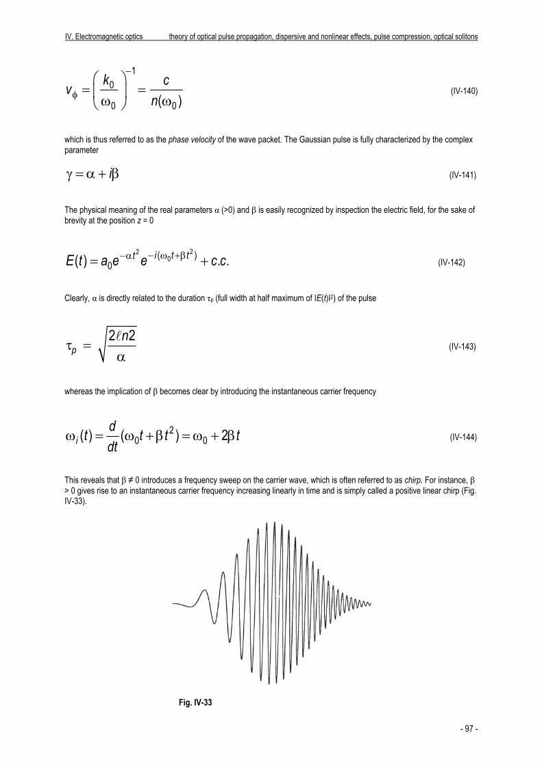
which is thus referred to as the phase velocity of the wave packet. The Gaussian pulse is fully characterized by the complex parameter

iγ = α + β (IV-141) The physical meaning of the real parameters α (>0) and β is easily recognized by inspection the electric field, for the sake of brevity at the position z = 0

− ω +β−α=22

0( )0 +( ) . .i t ttE t a e e c c (IV-142)

Clearly, α is directly related to the duration τp (full width at half maximum of IE(t)I2) of the pulse

2 2p

nτ =

αl

(IV-143)

whereas the implication of β becomes clear by introducing the instantaneous carrier frequency

20 0( ) ( ) 2i

dt t tdt

ω = ω +β = ω + βt (IV-144)

This reveals that β ≠ 0 introduces a frequency sweep on the carrier wave, which is often referred to as chirp. For instance, β > 0 gives rise to an instantaneous carrier frequency increasing linearly in time and is simply called a positive linear chirp (Fig. IV-33).

Fig. IV-33

- 97 -


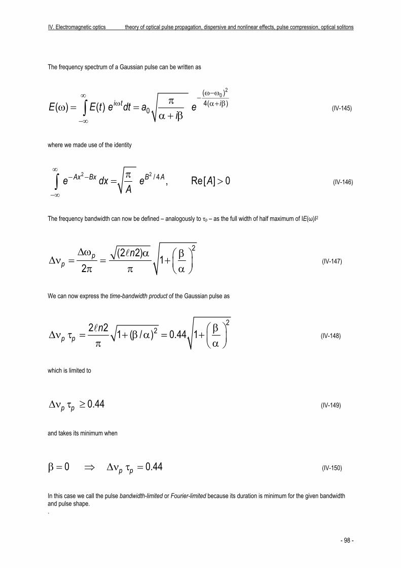
The frequency spectrum of a Gaussian pulse can be written as

ω−ω∞ −ω α+ β

−∞

πω = =

α + β∫2

0( )4( )

0( ) ( ) i t iE E t e dt a ei

(IV-145)

where we made use of the identity

2 2 / 4 , Re[ ]Ax Bx B Ae dx e A

A

∞− −

−∞

π=∫ 0> (IV-146)

The frequency bandwidth can now be defined – analogously to τp – as the full width of half maximum of IE(ω)I2

2(2 2) 12

pp

nΔω α β⎛ ⎞Δν = = + ⎜ ⎟π π α⎝ ⎠

l (IV-147)

We can now express the time-bandwidth product of the Gaussian pulse as

222 2 1 ( / ) 0.44 1p p

n β⎛ ⎞Δν τ = + β α = + ⎜ ⎟π α⎝ ⎠

l (IV-148)

which is limited to

0.44p pΔν τ ≥ (IV-149)

and takes its minimum when

0 p pβ = ⇒ Δν τ = 0.44 (IV-150)

In this case we call the pulse bandwidth-limited or Fourier-limited because its duration is minimum for the given bandwidth and pulse shape. .

- 98 -


The parameters of a Gaussian pulse with the initial parameters

in in in(0) iγ ≡ γ = α + β (IV-151) change upon propagation through a dispersive medium characterized by k2 according to (IV-137) as

2 22 2 2 21 1 2 2( ) (0)

in in

in in in inik z i k z

z⎛ ⎞α β

= − = − +⎜γ γ α +β α +β⎝ ⎠

⎟ (IV-152)

This expression, in combination with (IV-148) yields for a bandwidth-limited input pulse (βin = 0)

outout in

out in

0 ⎫β >⇒ τ > τ⎬

Δν = Δν ⎭ (IV-153)

Hence a bandwidth-limited pulse is temporally broadened upon propagation through a dispersive medium. From (IV-152) and (IV-143) we obtain

2

in( ) 1pD

zzL

⎛ ⎞τ = τ + ⎜ ⎟

⎝ ⎠ with

2in

2(4 n2) kDL τ=

l (IV-154a,b)

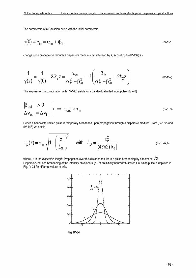
where LD is the dispersive length. Propagation over this distance results in a pulse broadening by a factor of 2 . Dispersion-induced broadening of the intensity envelope IE(t)I2 of an initially bandwidth-limited Gaussian pulse is depicted in Fig. IV-34 for different values of z/LD.

Fig. IV-34

- 99 -


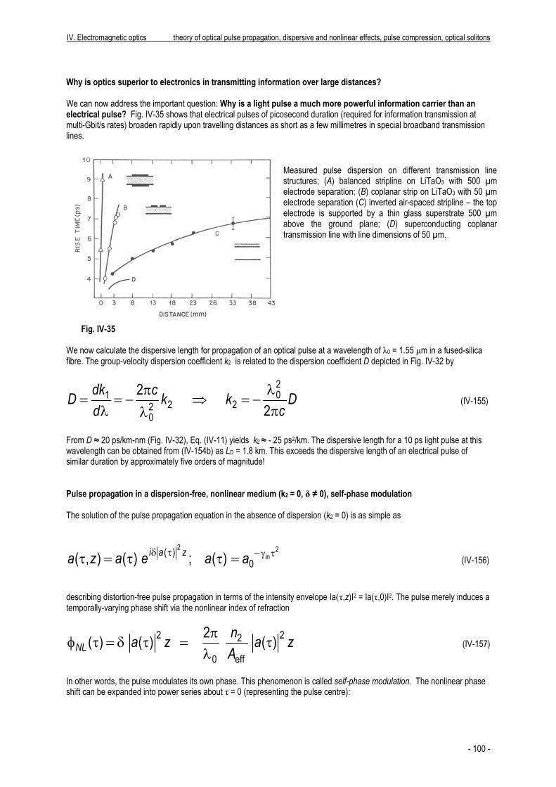
Why is optics superior to electronics in transmitting information over large distances? We can now address the important question: Why is a light pulse a much more powerful information carrier than an electrical pulse? Fig. IV-35 shows that electrical pulses of picosecond duration (required for information transmission at multi-Gbit/s rates) broaden rapidly upon travelling distances as short as a few millimetres in special broadband transmission lines. Fig. IV-35 Fig. IV-35

Measured pulse dispersion on different transmission line structures; (A) balanced stripline on LiTaO3 with 500 µm electrode separation; (B) coplanar strip on LiTaO3 with 50 µm electrode separation (C) inverted air-spaced stripline – the top electrode is supported by a thin glass superstrate 500 µm above the ground plane; (D) superconducting coplanar transmission line with line dimensions of 50 µm.

We now calculate the dispersive length for propagation of an optical pulse at a wavelength of λ0 = 1.55 μm in a fused-silica fibre. The group-velocity dispersion coefficient k2 is related to the dispersion coefficient D depicted in Fig. IV-32 by

201

2 220

22

dk cD k kd c

λπ= = − ⇒ = −

λ πλD (IV-155)

From D ≈ 20 ps/km-nm (Fig. IV-32), Eq. (IV-11) yields k2 ≈ - 25 ps2/km. The dispersive length for a 10 ps light pulse at this wavelength can be obtained from (IV-154b) as LD = 1.8 km. This exceeds the dispersive length of an electrical pulse of similar duration by approximately five orders of magnitude! Pulse propagation in a dispersion-free, nonlinear medium (k2 = 0, δ ≠ 0), self-phase modulation The solution of the pulse propagation equation in the absence of dispersion (k2 = 0) is as simple as

δ τ −γ ττ = τ τ =2 2

in( )0( , ) ( ) ; ( )i a za z a e a a (IV-156)

describing distortion-free pulse propagation in terms of the intensity envelope Ia(τ,z)I2 = Ia(τ,0)I2. The pulse merely induces a temporally-varying phase shift via the nonlinear index of refraction

πφ τ = δ τ = τ

λ2 22

0 eff

2( ) ( ) ( )NLna z aA

z (IV-157)

In other words, the pulse modulates its own phase. This phenomenon is called self-phase modulation. The nonlinear phase shift can be expanded into power series about τ = 0 (representing the pulse centre):

- 100 -


2NL NL NL( ) ...φ τ = Δφ −β τ (IV-158a)

where

NL 2 NL0

2pn zπ

Δφ =λ

I (IV-158b) (IV-158b) π

Δφ =λ

I

is the peak nonlinear phase shift with Ip = Ia0I2/Aeff representing the peak intensity of the pulse and is the peak nonlinear phase shift with Ip = Ia0I2/Aeff representing the peak intensity of the pulse and

− α τ

τ=

⎛ ⎞φβ = − = − δ⎜ ⎟

τ τ⎝ ⎠

2in

2 22 2NL

0 NL2 20

1 12 2NL

d da z ed d

NLin 2 NL 2 NL2 2

0 0

2 8 2 4 22 p pp p

zn nn z nπ π= α = = Δφ

λ λτ τl lI I (IV-158c)

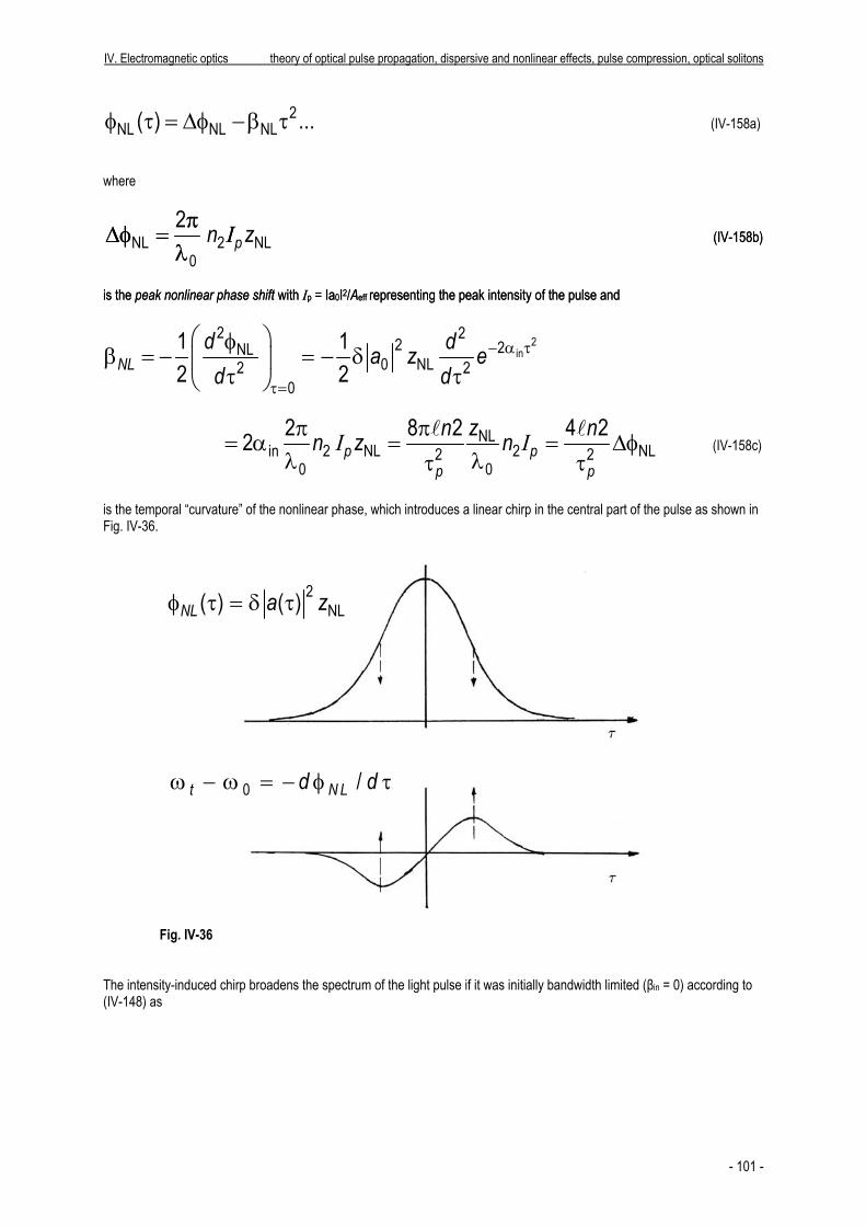
is the temporal “curvature” of the nonlinear phase, which introduces a linear chirp in the central part of the pulse as shown in Fig. IV-36.

φ τ = δ τ 2NL( ) ( )NL a z

0 /t N Ld dω − ω = − φ τ

Fig. IV-36 The intensity-induced chirp broadens the spectrum of the light pulse if it was initially bandwidth limited (βin = 0) according to (IV-148) as

- 101 -


2NL

in in 2in 0

2in NL

( ) 1 1 4

1 4

NLNL p

zL n⎛ ⎞⎛ ⎞β

Δν ≈ Δν + = Δν + π⎜ ⎟⎜ ⎟α λ⎝ ⎠ ⎝

= Δν + Δφ

I =⎠ (IV-159)

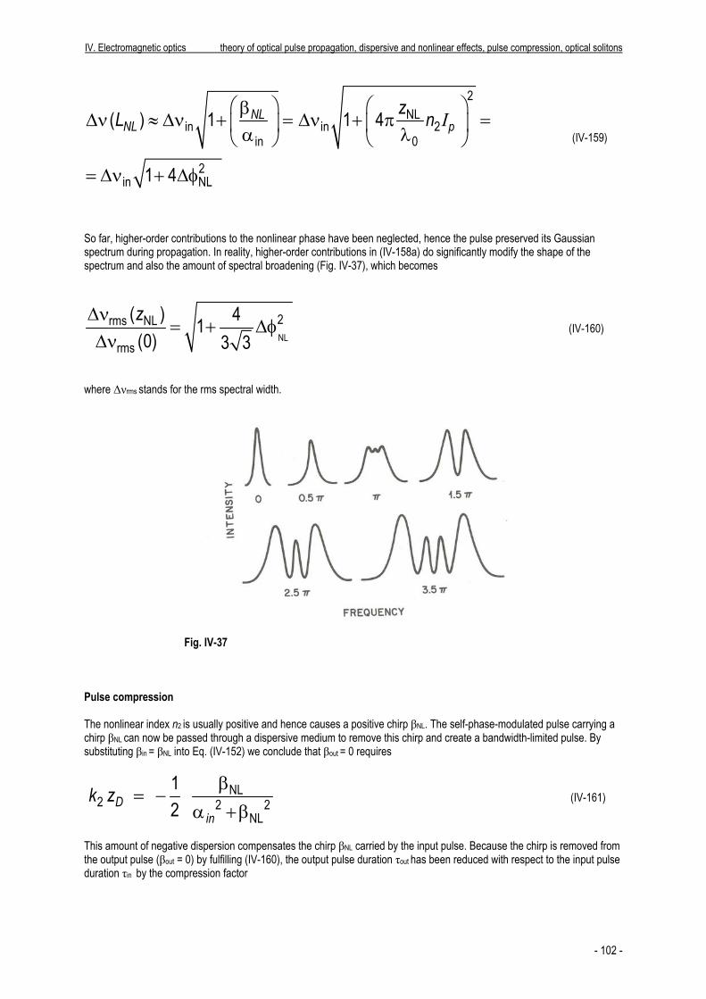
So far, higher-order contributions to the nonlinear phase have been neglected, hence the pulse preserved its Gaussian spectrum during propagation. In reality, higher-order contributions in (IV-158a) do significantly modify the shape of the spectrum and also the amount of spectral broadening (Fig. IV-37), which becomes

NL

2rms NL

rms

( ) 41(0) 3 3zΔν

= + ΔφΔν

(IV-160)

where Δνrms stands for the rms spectral width.

Fig. IV-37 Pulse compression The nonlinear index n2 is usually positive and hence causes a positive chirp βNL. The self-phase-modulated pulse carrying a chirp βNL can now be passed through a dispersive medium to remove this chirp and create a bandwidth-limited pulse. By substituting βin = βNL into Eq. (IV-152) we conclude that βout = 0 requires

NL2 2

NL

12D

ink z β

= −α +β 2 (IV-161)

This amount of negative dispersion compensates the chirp βNL carried by the input pulse. Because the chirp is removed from the output pulse (βout = 0) by fulfilling (IV-160), the output pulse duration τout has been reduced with respect to the input pulse duration τin by the compression factor

- 102 -


Pulse compression factor 2rms NLinNL

rmsout

( ) 41(0) 3 3zΔντ

= ≈ = + ΔφΔντ

(IV-162)

In reality, the nonlinear medium is also dispersive and dispersion broadens the pulse temporally during the buildup of the nonlinear phase shift. For a positive dispersion, k2 > 0, this effect smoothens the structure in Fig. IV-37 and linearises the temporal chirp, leading thereby to a better quality of the compressed pulses2. For a propagation length in the nonlinear medium that satisfies zNL < LD, however, Eq. (IV-162) remains a good approximation. The pulse shortening originating from self-phase modulation followed by dispersive delay plays a central role in modern ultrashort-pulse laser systems. Pulse propagation in a dispersive, nonlinear medium with k2 < 0, δ > 0: optical solitons Nonlinearity and dispersion of opposite sign, if acting after each other, may result in shortening of an optical pulse. Here we note that if they act simultaneously, the pulse broadening that k2 ≠ 0 tends to induce in the absence of a nonlinearity can be eliminated as a result of the interplay between the dispersive and nonlinear effects. For k2 < 0, δ > 0, the hyperbolic secant pulse of the form

⎛ ⎞ττ = ⎜ ⎟τ⎝ ⎠

/ 20

0( , ) sech Diz La z a e with

20

2DL

kτ

= (IV-163a,b)

constitutes a solution of the nonlinear propagation equation, if the peak power of the pulse satisfies

= ≈δτ δτ

2 2 20 2

0

3.11

p

k ka 2

(IV-164)

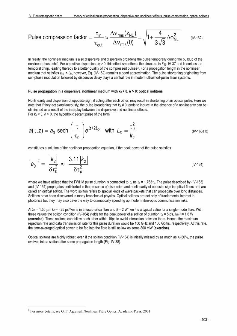
where we have utilized that the FWHM pulse duration is connected to τ0 as τp = 1.763τ0. The pulse described by (IV-163) and (IV-164) propagates undistorted in the presence of dispersion and nonlinearity of opposite sign in optical fibers and are called an optical soliton. The word soliton refers to special kinds of wave packets that can propagate over long distances. Solitons have been discovered in many branches of physics. Optical solitons are not only of fundamental interest in photonics but they may also pave the way to dramatically speeding up modern fibre-optic communication links. At λ0 = 1.55 μm k2 ≈ - 25 ps2/km is in a fused-silica fibre and δ = 2 W-1km-1 is a typical value for a single-mode fibre. With these values the soliton condition (IV-164) yields for the peak power of a soliton of duration τp = 5 ps, Iv0I2 ≈ 1.6 W (exercise). These solitons can follow each other within 10ps to avoid interaction between them. Hence, the maximum repetition rate and data transmission rate for this pulse duration would be 100 GHz and 100 Gbit/s, respectively. At this rate, the time-averaged optical power to be fed into the fibre is still as low as some 800 mW (exercise). Optical solitons are highly robust: even if the soliton condition (IV-164) is initially missed by as much as +/-50%, the pulse evolves into a soliton after some propagation length (Fig. IV-38).

2 For more details, see G. P. Agrawal, Nonlinear Fibre Optics, Academic Press, 2001

- 103 -


Soliton evolution

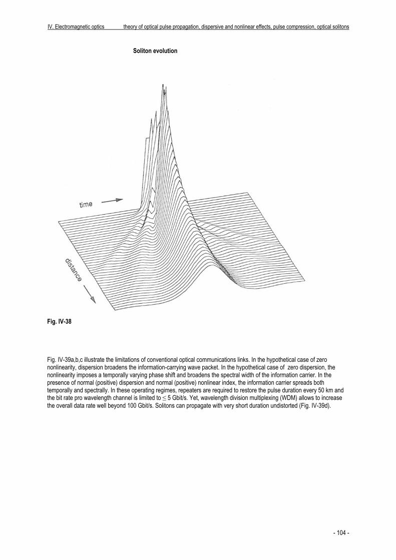
Fig. IV-38 Fig. IV-39a,b,c illustrate the limitations of conventional optical communications links. In the hypothetical case of zero nonlinearity, dispersion broadens the information-carrying wave packet. In the hypothetical case of zero dispersion, the nonlinearity imposes a temporally varying phase shift and broadens the spectral width of the information carrier. In the presence of normal (positive) dispersion and normal (positive) nonlinear index, the information carrier spreads both temporally and spectrally. In these operating regimes, repeaters are required to restore the pulse duration every 50 km and the bit rate pro wavelength channel is limited to ≤ 5 Gbit/s. Yet, wavelength division multiplexing (WDM) allows to increase the overall data rate well beyond 100 Gbit/s. Solitons can propagate with very short duration undistorted (Fig. IV-39d).

- 104 -


k2 < 0, δ > 0 ⇒ soliton propagation

2 0, 0k ≠ δ =

2 0, 0k = δ ≠

2 0, 0k > δ >

< δ >2 0, 0k

Fig. IV-39

- 105 -


- 106 -

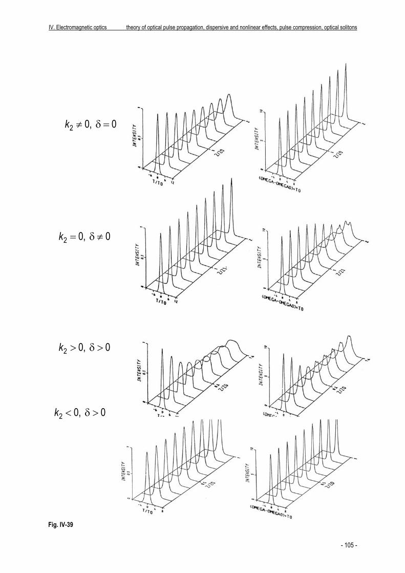
Long-distance optical data transmission experiments are performed in fibre loops (Fig. IV-40).

→⏐ ⏐← 100 ps 10 Gbit/s ⇒ Fig. IV-40 In soliton communication, the data rate per channel might eventually reach or possibly exceed 100 Gbit/s, holding promise for multi-Tbit/s transmission rates in combination with WDM. Most importantly, they obviate the need for complicated repeaters. They merely require reamplification to compensate for propagation losses, which can be accomplished by erbium-doped fibre amplifiers operating at λ0 = 1.55 μm.

Theory of optical pulse propagation - LMU

Documents

Transcript of Theory of optical pulse propagation - LMU