
Theory of Fuzzy Information Granulation: Contributions to ...
300
UNIVERSITÀ DEGLI STUDI DI BARI FACOLTÀ DI SCIENZE MM.FF.NN DIPARTIMENTO DI INFORMATICA Theory of Fuzzy Information Granulation: Contributions to Interpretability Issues Autore: Corrado Mencar Tutor: Prof. Anna Maria Fanelli Tesi sottomessa in parziale accoglimento dei requisiti per il conseguimento del titolo di DOTTORE DI RICERCA IN INFORMATICA Dicembre 2004 DOTTORATO DI RICERCA IN INFORMATICA — XVI CICLO
Transcript of Theory of Fuzzy Information Granulation: Contributions to ...
UNIVERSITÀ DEGLI STUDI DI BARI
FACOLTÀ DI SCIENZE MM.FF.NN DIPARTIMENTO DI INFORMATICA
Theory of Fuzzy Information Granulation: Contributions to Interpretability Issues
Autore: Corrado Mencar
Tutor: Prof. Anna Maria Fanelli
Tesi sottomessa in parziale accoglimento dei requisiti per il conseguimento del titolo di
DOTTORE DI RICERCA IN INFORMATICA
Dicembre 2004
DOTTORATO DI RICERCA IN INFORMATICA — XVI CICLO

UNIVERSITY OF BARI
FACULTY OF SCIENCE DEPARTMENT OF INFORMATICS
Theory of Fuzzy Information Granulation: Contributions to Interpretability Issues
Author: Corrado Mencar
Supervisor: Prof. Anna Maria Fanelli
A thesis submitted in partial fulfillment of the requirements for the degree of
DOCTOR OF PHILOSPHY IN INFORMATICS
December 2004
PHD COURSE IN INFORMATICS — CYCLE XVI

Abstract
Granular Computing is an emerging conceptual and computationalparadigm for information processing, which concerns representationand processing of complex information entities called “informationgranules” arising from processes of data abstraction and knowledgederivation. Within Granular Computing, a prominent position is as-sumed by the “Theory of Fuzzy Information Granulation” (TFIG)whose centrality is motivated by the ability of representing and process-ing perception-based granular information. A key aspect of TFIG isthe process of data granulation in a form that is interpretable by hu-man users, which is achieved by tagging granules with linguisticallymeaningful (i.e. metaphorical) labels belonging to natural language.However, the process of interpretable information granulation is nottrivial and poses a number of theoretical and computational issuesthat are subject of study in this thesis.In the first part of the thesis, interpretability is motivated from severapoints of view, thus endowing with a robust basis for justifying itsstudy within the TFIG. On the basis of this analysis, the constraint-based approach is recognized as an effective means for characterizingthe intuitive notion of interpretability. Interpretability constraintsknown in literature are hence deeply surveyed with a homogeneousmathematical formalization and critically reviewed from several per-spectives encompassing computational, psychological, and linguisticconsiderations.In the second part of the thesis some specific issues on interpretabil-ity constraints are addressed and novel theoretical contributions areproposed. More specifically, two main results are achieved: the firstconcerns the quantification of the distinguishability constraint throughthe possibility measure, while the second regards the formalization ofa new measure to quantify information loss when information granulesare used to design fuzzy models.The third part of the thesis is concerned with the development ofnew algorithms for interpretable information granulation. Such algo-rithms enable the generation of fuzzy information granules that ac-curately describe available data and are properly represented both interms of quantitative and qualitative linguistic labels. These informa-tion granules can be used as building blocks for designing neuro-fuzzymodels through neural learning. To avoid interpretability loss due tothe adaptation process, a new architecture for neuro-fuzzy networksand its learning algorithm are proposed with the specific aim of inter-pretability protection.
ii

Contents
Contents iii
Acknowledgements ix
Preface xi
I Interpretability Issues in Fuzzy Information Gran-ulation 1
1 Granular Computing 31.1 The emergence of Granular Computing . . . . . . . . . . . . . 3
1.1.1 Defining Granular Computing . . . . . . . . . . . . . . 51.1.2 Information Granulation . . . . . . . . . . . . . . . . . 6
1.2 Theory of Fuzzy Information Granulation . . . . . . . . . . . . 91.2.1 Granulation as a cognitive task . . . . . . . . . . . . . 111.2.2 Symbolic representation of fuzzy information granules . 121.2.3 Interpretability of fuzzy information granules . . . . . . 16
2 Interpretability Constraints for Fuzzy Information Granules 212.1 Introduction . . . . . . . . . . . . . . . . . . . . . . . . . . . . 212.2 Constraints on Fuzzy sets . . . . . . . . . . . . . . . . . . . . 222.3 Constraints on Frames of Cognition . . . . . . . . . . . . . . . 302.4 Constraints on Fuzzy Information Granules . . . . . . . . . . . 492.5 Constraints on Rules . . . . . . . . . . . . . . . . . . . . . . . 532.6 Constraints on Fuzzy Models . . . . . . . . . . . . . . . . . . . 582.7 Constraints on Fuzzy Model Adaption . . . . . . . . . . . . . 782.8 Final remarks . . . . . . . . . . . . . . . . . . . . . . . . . . . 83
iii
Contents
II Theoretical Contributions to Interpretabilty inFuzzy Information Granulation 85
3 Distinguishability Quantification 873.1 Introduction . . . . . . . . . . . . . . . . . . . . . . . . . . . . 873.2 Distinguishability measures . . . . . . . . . . . . . . . . . . . 89
3.2.1 Similarity measure . . . . . . . . . . . . . . . . . . . . 893.2.2 Possibility measure . . . . . . . . . . . . . . . . . . . . 913.2.3 Other distinguishability measures . . . . . . . . . . . . 94
3.3 Theorems about Similarity and Possibility measures . . . . . . 993.4 Theorem about distinguishability improvement . . . . . . . . . 1083.5 Final remarks . . . . . . . . . . . . . . . . . . . . . . . . . . . 110
4 Interface Optimality 1134.1 Introduction . . . . . . . . . . . . . . . . . . . . . . . . . . . . 1134.2 Fuzzy Interfaces . . . . . . . . . . . . . . . . . . . . . . . . . . 116
4.2.1 Input Interface . . . . . . . . . . . . . . . . . . . . . . 1164.2.2 Processing Module . . . . . . . . . . . . . . . . . . . . 1174.2.3 Output Interface . . . . . . . . . . . . . . . . . . . . . 118
4.3 Theorems about optimality for Input Interfaces . . . . . . . . 1194.3.1 Bi-monotonic fuzzy sets . . . . . . . . . . . . . . . . . 1204.3.2 Optimality conditions . . . . . . . . . . . . . . . . . . 121
4.4 A measure of optimality for Output Interfaces . . . . . . . . . 1244.4.1 Optimality Degree . . . . . . . . . . . . . . . . . . . . 1244.4.2 Illustrative examples . . . . . . . . . . . . . . . . . . . 127
4.5 Final remarks . . . . . . . . . . . . . . . . . . . . . . . . . . . 131
III Algorithms for Deriving Interpretable Fuzzy In-formation Granules 133
5 Gaussian Information Granulation 1355.1 Introduction . . . . . . . . . . . . . . . . . . . . . . . . . . . . 1355.2 A method of Information Granulation with Gaussian fuzzy sets138
5.2.1 Problem formulation . . . . . . . . . . . . . . . . . . . 1385.2.2 Analysis of the solution . . . . . . . . . . . . . . . . . . 1415.2.3 Fuzzy model design with Gaussian granules . . . . . . 142
5.3 Illustrative examples . . . . . . . . . . . . . . . . . . . . . . . 1435.3.1 Information granulation of postal addresses . . . . . . . 1445.3.2 Prediction of automobile fuel consumption . . . . . . . 148
5.4 Final remarks . . . . . . . . . . . . . . . . . . . . . . . . . . . 153
iv

Contents
6 Minkowski Information Granulation 1556.1 Introduction . . . . . . . . . . . . . . . . . . . . . . . . . . . . 1556.2 A method for Information Granulation through Minkowski
fuzzy clustering . . . . . . . . . . . . . . . . . . . . . . . . . . 1576.2.1 Minkowski Fuzzy C-Means . . . . . . . . . . . . . . . . 1576.2.2 Generation of Information Granules . . . . . . . . . . . 159
6.3 Illustrative example . . . . . . . . . . . . . . . . . . . . . . . . 1646.4 Final remarks . . . . . . . . . . . . . . . . . . . . . . . . . . . 171
7 Information Granulation through Prediction Intervals 1737.1 Introduction . . . . . . . . . . . . . . . . . . . . . . . . . . . . 1737.2 A method of Information Granulation through Prediction In-
tervals . . . . . . . . . . . . . . . . . . . . . . . . . . . . . . . 1757.2.1 Reference Model . . . . . . . . . . . . . . . . . . . . . 1757.2.2 Prediction interval derivation . . . . . . . . . . . . . . 176
7.3 Illustrative examples . . . . . . . . . . . . . . . . . . . . . . . 1787.3.1 Nonlinear function approximation . . . . . . . . . . . . 1787.3.2 Ash combustion properties prediction . . . . . . . . . . 180
7.4 Final remarks . . . . . . . . . . . . . . . . . . . . . . . . . . . 180
8 Information Granulation through Double Clustering 1838.1 Introduction . . . . . . . . . . . . . . . . . . . . . . . . . . . . 1838.2 The Double Clustering Framework . . . . . . . . . . . . . . . 185
8.2.1 Fuzzy Double Clustering . . . . . . . . . . . . . . . . . 1908.2.2 Crisp Double Clustering . . . . . . . . . . . . . . . . . 1938.2.3 DCClass . . . . . . . . . . . . . . . . . . . . . . . . . . 194
8.3 Illustrative examples . . . . . . . . . . . . . . . . . . . . . . . 1968.3.1 Granulation example . . . . . . . . . . . . . . . . . . . 1968.3.2 Fuzzy Diagnosis . . . . . . . . . . . . . . . . . . . . . . 204
8.4 Final remarks . . . . . . . . . . . . . . . . . . . . . . . . . . . 205
9 Refinement of Interpretable Information Granules throughNeural Learning 2119.1 Introduction . . . . . . . . . . . . . . . . . . . . . . . . . . . . 2119.2 A neuro-fuzzy network to learn interpretable information gran-
ules . . . . . . . . . . . . . . . . . . . . . . . . . . . . . . . . . 2149.2.1 The subspace of interpretable configurations . . . . . . 2149.2.2 The Neuro-Fuzzy architecture . . . . . . . . . . . . . . 2219.2.3 The Neuro-Fuzzy learning scheme . . . . . . . . . . . . 225
9.3 Illustrative examples . . . . . . . . . . . . . . . . . . . . . . . 2319.3.1 Non-linear system identification . . . . . . . . . . . . . 231
v

Contents
9.3.2 Fuzzy Medical Diagnosis . . . . . . . . . . . . . . . . . 2339.4 Final remarks . . . . . . . . . . . . . . . . . . . . . . . . . . . 241
IV Conclusions and Future Research 243
List of Figures 249
List of Tables 255
Bibliography 257
vi

It is not a case that ‘wife’ and ‘life’are almost identical words.And I know the reason.
To Laura, with love.
vii

viii

Acknowledgements
This work is the result of three years of research efforts during my Ph.D.studentship. Of course, most of such work would have not been possiblewithout the support of many people that I wish to thank. First of all, mygratitude goes to my supervisor and tutor, prof. Anna Maria Fanelli, whosupported me all the time by guiding my work on the right direction. I amalso thankful to her for patiently reviewing and improving my work. Last,but not least, she established a pleasant working environment that I foundabsolutely beneficial for my work.I express my gratitude also to prof. Andrzej Bargiela, of Nottingham
Trent University (Nottingham, United Kingdom) for his fruitful interactionwithin my research work, which stimulated the development of new contri-butions that are part of this thesis. He also shed light on new ideas forfuture scientific investigation. I am grateful also to my co-tutor, prof. Do-nato Malerba, for his suggestions that turned out to be useful for this workas well as for future research.Many thanks also to my colleagues Dr. Giovanna Castellano and Dr. Ciro
Castiello of the Department of Informatics, University of Bari. Giovanna gaveme useful suggestions for the development of my work and for supporting thereview of the final thesis. Ciro enlightened me on many philosophical facetsof our common research interests.Finally, a loveful thank to my wife for always standing by me all the time,
especially in the toughest moments.
ix

Acknowledgements
x
Preface
Granular Computing is an emerging conceptual and computational paradigmfor information processing, which plays a fundamental role within the field ofComputational Intelligence. It concerns representing and processing complexinformation entities called “information granules”, which arise in the processof abstraction of data and derivation of knowledge from information. WithinGranular Computing, a number of formal frameworks have been developed,among which the “Theory of Fuzzy Information Granulation” (TFIG) as-sumes a prominent position. The centrality of TFIG is motivated by theability of representing and processing perception-based granular information,thus providing an effective model of human reasoning and cognition. A keyaspect of TFIG is the granulation of data in a form that is readily understand-able by human users. Interpretability of the resulting fuzzy information gran-ules is usually achieved by tagging them with linguistically meaningful (i.e.metaphorical) labels, belonging to natural language. However, the semanticsof information granules resulting from unconstrained granulation processeshardly matches metaphors of linguistic labels. As a consequence, an interest-ing research issue arises in the development of fuzzy information granulationmethods that ensure interpretability of the derived granules. The definitionof such methods cannot be separated from a deep theoretical study about theblurred notion of interpretability itself.This thesis provides some contributions to the study of interpretability
issues in the context of TFIG.The introductory part of the thesis aims at motivating and defining the
notion of “interpretability” within TFIG. Specifically, the First Chapter in-troduces the notion of interpretability in TFIG from several points of view,including computational, epistemological and linguistic ones. In the attemptto formalize the notion of interpretability in Fuzzy Information Granulation,the constraint-based approach is investigated. As there is not an universallyaccepted set of constraints that characterize the notion of interpretability,in the Second Chapter a corpus of interpretability constraints is collected,homogeneously treated and critically reviewed. Both the Chapters trace an
xi
Preface
introductory path that serves as a basis for novel theoretical contributions inthe field of Interpretable Fuzzy Information Granulation, and supplies a for-mal support to design new algorithms for the extraction and refinement ofinterpretable information granules.Based on this preliminary study, some theoretical contributions are pro-
posed in the second part of the thesis, by addressing specific issues on in-terpretability constraints. The first contribution, introduced in the ThirdChapter, is focused on the “Distinguishability” constraint, which is deeplysurveyed, with special attention to the measures that quantify its fulfillment.More specifically, two measures, namely “similarity” and “possibility” arecompared from a theoretical point of view. As a result, the possibility measureemerges as a valid tool to quantify distinguishability with a clear semanticsand a low computational cost.A second theoretical contribution is presented in the Fourth Chapter,
which is concerned with the “Information Equivalence Criterion” constraint.A new mathematical characterization is provided for this constraint, whichapplies to input and output interfaces of a fuzzy model. It is proved that,for a specific class of input interfaces, the Information Equivalence Criterionis met under mild conditions. For output interfaces, which can hardly ful-fill such constraint, a measure is defined to quantify the degree of fulfillment.Such measure can be conveniently used to compare different output interfaces,thus serving as a tool for designing interpretable fuzzy models.The third part of the thesis is concerned with the development of algo-
rithms for interpretable fuzzy information granulation. The first algorithm,presented in the Fifth Chapter, wraps a fuzzy clustering scheme to achieve in-terpretable granulation by solving a constrained quadratic programming prob-lem. Key features of such algorithm are a low computational cost and acompact representation of the resulting granules.The Sixth Chapter introduces an algorithm for information granulation
to generate information granules in form of hyper-boxes, thus providing aninterval-based quantification of data. The granulation algorithm extends astandard fuzzy clustering algorithm to deal with Minkowski metrics of highorder. The algorithm produces boxlike granules whose shape may be distortedby some factors. Such distortion effects are deeply examined and properlyquantified, in order to analytically evaluate the effectiveness of the granulationprocess.Interval representation of information granules has been adopted also to
extend the rule-based formalization of knowledge base of some fuzzy inferencesystems in order to improve its interpretability. In the Seventh Chapter,such extension is obtained with an algorithm for deriving prediction intervalsfor fuzzy models acquired from data, and its effectiveness is illustrated on a
xii
Preface
real-world complex prediction problem.All such algorithms are especially useful in applicative contexts where
information granulation is necessary to represent fuzzy quantities (i.e. fuzzynumbers or fuzzy vectors). In other applications, qualitative representationsof information granules are rather preferred. Qualitative information gran-ules represent information in terms of natural language terms — such as ad-jectives, adverbs etc. — rather than quantitative labels. Although less precise,qualitative information granules are at the basis of human perception, reason-ing and communication; hence it is highly desirable that machine could ac-quire knowledge expressible in the same terms. This is not a trivial task, how-ever, since interpretability constraints are very stringent and require specifi-cally suited algorithms for qualitative information granulation.In the Eighth Chapter an algorithmic framework is proposed for quali-
tative information granulation. It is called “Double Clustering” because itis pivoted on two clustering algorithms that can be chosen on the basis ofapplicative considerations. The proper combination of the two clustering al-gorithms — the former aimed at discovering hidden relationships among dataand the latter at defining interpretable fuzzy sets — enables the generation offuzzy information granules that properly describe available data and can beconveniently represented by means of qualitative linguistic terms. Some ofthese instances are described in detail in the Chapter, and their effectivenessis assessed on some benchmark problems.Information granules acquired from data can be used in fuzzy models to
solve problems of prediction, classification, system identification etc.. A com-mon and effective type of fuzzy model is the “Fuzzy Inference System”, whichenables the representation of the embodied knowledge in form of a rule base,being each rule explicitly defined by means of fuzzy information granules.The key feature of Fuzzy Inference System is its possibility of being translatedinto a neural network that can be trained to acquire an unknown functionalrelationship from data. However, a classical unconstrained neural learningscheme can easily hamper the interpretability of the model’s knowledge base,since interpretability constraints ace be easily violated during the trainingprocess. To avoid the invalidation of interpretability in adapting informa-tion granules, a novel neural architecture is proposed in the Ninth Chapter— together with an appropriate learning scheme based on gradient descent.The resulting neural model enables interpretability protection in all stages ofneural learning. The correctness of the proposed architecture in preservinginterpretability constraints is proved formally and experimentally verified ona set of benchmark problems.All the contributions reported in this work finally emerge as a unified
framework for extraction and refinement of interpretable fuzzy information
xiii

Preface
granules. The research direction cast by this work is however by no wayexhausted, but it is open to further improvements and extensions in futurescientific investigations as highlighted in the conclusive part of the thesis.Most of the work in this thesis has been presented in peer-reviewed in-
ternational and national conferences, and has been published, or is underconsideration for publication, in international journals. The publications re-lated to this thesis are listed below:Papers on National and International Journals
• G. Castellano, A.M. Fanelli, C. Mencar, “A Neuro-Fuzzy Network To Gen-erate Human Understandable Knowledge From Data” in COGNITIVE SYS-TEMS RESEARCH 3(2):125-144, Special Issue on Computational CognitiveModeling, Elsevier, 2002, ISSN: 1389-0417
• G. Castellano, A.M. Fanelli, C. Mencar, “Generation Of Interpretable FuzzyGranules By A Double-Clustering Technique” in ARCHIVES OF CON-TROL SCIENCES 12(4):397-410, Special Issue on Granular Computing,Silesian University of Technology, 2002, ISSN: 1230-2384
• G. Castellano, A.M. Fanelli, C. Mencar “Fuzzy Information Granulation- A Compact, Transparent and Efficient representation” in JOURNAL OFADVANCED COMPUTATIONAL INTELLIGENCE AND INTELLIGENTINFORMATICS (JACIII), vol.7(2):160-168, June 2003, Fuji Technology Press,ISSN: 1343-0130
• G. Castellano, C. Castiello, A.M. Fanelli, C. Mencar, “Knowledge Discoveryby a Neuro-Fuzzy Modeling Framework”, in FUZZY SETS & SYSTEMS,VOL. 149(1):187-207, Special Issue on Fuzzy Sets in Knowledge Discovery,Elsevier, ISSN: 0165-0114
• C. Mencar, G. Castellano, A.M. Fanelli, “Deriving Prediction Intervals forNeurofuzzy Networks”, in MATHEMATICAL AND COMPUTER MOD-ELLING: AN INTERNATIONAL JOURNAL, Elsevier, in press, ISSN 0895-7177 (invited paper)
• G. Castellano, C. Castiello, A.M. Fanelli, C. Mencar, “Una MetodologiaNeuro-Fuzzy per la Predizione delle Proprietà dei Rifiuti Industriali”, inINTELLIGENZA ARTIFICIALE, vol. 1(3):27-35, ISSN: 1724-8035
Chapters in International Books
xiv

Preface
• C. Mencar, “Extracting Interpretable Fuzzy Knowledge from Data” in B.Apolloni, F. Kurfess (eds.), “FROM SYNAPSES TO RULES: DISCOVER-ING SYMBOLIC RULES FROMNEURAL PROCESSED DATA”, pp. 109-116, Kluwer Academic/Plenum Publishers, New York, 2002, ISBN: 0306474026(invited paper)
• G. Castellano, A.M. Fanelli, C. Mencar, “Design of Transparent Mam-dani Fuzzy Inference Systems”, in A. Abraham, M. Köppen, K. Franke(eds.), “DESIGN AND APPLICATION OF HYBRID INTELLIGENT SYS-TEMS”, pp. 468-476, IOS Press, The Netherlands, 2003, ISBN: 1-58603-394-8
• G. Castellano, A.M. Fanelli, C. Mencar, “Bi-monotonic Fuzzy Sets Lead toOptimal Fuzzy Interfaces”, in F. Masulli, A. Petrosino (eds.) “LECTURENOTES IN COMPUTER SCIENCE” (Proceedings of the INTENATIONALWORKSHOP ON FUZZY LOGIC AND APPLICATIONS (WILF 2003)),Springer-Verlag, 9-11 oct. 2003, Istituto Italiano Studi Filosofici, Naples,Italy, in press, Springer-Verlag, in press
• G. Castellano, A.M. Fanelli, C. Mencar, “Deriving Prediction Intervals forNeurofuzzy Networks”, in T.E. Simos (ed.), COMPUTATIONAL METH-ODS IN SCIENCES AND ENGINEERING (ICCMSE 2003), pp. 104-109,World Scientific, Kastoria, Greece, 12-16 sept. 2003, ISBN 981-238-595-9
Papers on National and International Conference Proceedings
• G. Castellano, A.M. Fanelli, C. Mencar, “Discovering Classification Rulesfrom Neural Processed Data” in atti del VIII CONVEGNO DELL’ASSO-CIAZIONE ITALIANA PER L’INTELLIGENZA ARTIFICIALE (AI*IA),pp. 473-482, Siena, Italy, 10-13 sept. 2002
• G. Castellano, A.M. Fanelli, C. Mencar, “A Double-Clustering Approach forInterpretable Granulation of Data”, in Proceedings of 2ND IEEE INTER-NATIONAL CONFERENCE ON SYSTEMS, MAN AND CYBERNETICS(IEEE SMC’02), Yasmine Hammamet, Tunisy, 6-9 oct. 2002., ISBN 2-9512309-4-X
• G. Castellano, A.M. Fanelli, C. Mencar, “A Compact Gaussian Represen-tation of Fuzzy Information Granules” in Proceedings of JOINT 1ST IN-TERNATIONAL CONFERENCE ON SOFT COMPUTING AND INTEL-LIGENT SYSTEMS AND 3RD INTERNATIONAL SYMPOSIUM ON AD-VANCED INTELLIGENT SYSTEMS (SCIS&ISIS 2002), Tsukuba, Japan,21-25 oct. 2002. Excellent Presentation Award.
xv
Preface
• G. Castellano, A.M. Fanelli, C. Mencar, “Discovering human understand-able fuzzy diagnostic rules from medical data” in Proceedings of EURO-PEAN SYMPOSIUM ON INTELLIGENT TECHNOLOGIES, HYBRIDSYSTEMS AND THEIR IMPLEMENTATION ON SMART ADAPTIVESYSTEMS (EUNITE 2003), pp. 227-233, Oulu, Finland, 10-12 july 2003
• G. Castellano, A.M. Fanelli, C. Mencar, “Fuzzy Granulation of Multidimen-sional Data by a Crisp Double Clustering algorithm”, in Proceedings of the7THWORLDMULTI-CONFERENCE ON SYSTEMICS, CYBERNETICSAND INFORMATICS (SCI 2003), pp. 372-377, Orlando, Fl, USA, 27-30july 2003, ISBN 980-6560-01-9
• G. Castellano, C. Castiello, A.M. Fanelli, C. Mencar, “Discovering Predic-tion Rules by a Neuro-Fuzzy Modelling Framework”, in Proceedings of 7THINTERNATIONAL CONFERENCE ON KNOWLEDGE-BASED INTEL-LIGENT INFORMATION & ENGINEERING SYSTEMS (KES 2003), vol.1, pp. 1242-1248, Springer, Oxford, UK, 3-5 sept. 2003, ISBN 3-540-40803-7
• G. Castellano, A.M. Fanelli, C. Mencar, “DCClass: A Tool to Extract Hu-man Understandable Fuzzy Information Granules for Classification”, in Pro-ceedings of the 4TH INTERNATIONAL SYMPOSIUM ON ADVANCEDINTELLIGENT SYSTEMS (SCIS&ISIS 2003), pp. 376-379, Jeju Island,Korea, 25-28 sept. 2003
• G. Castellano, A.M. Fanelli, C. Mencar, “A Fuzzy Clustering Approach forMining Diagnostic Rules”, in Proceedings of 2003 IEEE INTERNATIONALCONFERENCE ON SYSTEMS, MAN & CYBERNETICS (IEEE SMC’03),vol. 1, pp. 2007-2012, 5—8 oct. 2003 — Hyatt Regency, Washington, D.C.,USA, ISBN 0-7803-7952-7
• C. Mencar, A. Bargiela, G. Castellano, A.M. Fanelli, “Interpretable In-formation Granules with Minkowski FCM ”, in Proceedings of the CON-FERENCE OF NORTH AMERICAN FUZZY INFORMATION SOCIETY(NAFIPS2004), pp. 456-461, 27-30 june 2004, Banff, Alberta, Canada (BestStudent Paper Citation), ISBN 0-7803-8377-X
• G. Castellano, A.M. Fanelli, C. Mencar, “Optimality Degree Measurement inFuzzy System Interfaces”, in Proceedings of EUROPEAN SYMPOSIUMONINTELLIGENT TECHNOLOGIES, HYBRID SYSTEMS AND THEIR IM-PLEMENTATION ON SMART ADAPTIVE SYSTEMS (EUNITE 2004),pp. 443-451, 10-12 june 2004, Aachen, Germany
xvi

Preface
• G. Castellano, A.M. Fanelli, C. Mencar, “An Optimality Criterion for FuzzyOutput Interfaces”, in Proceedings of IEEE CONFERENCE ON INTELLI-GENT SYSTEMS DESIGN AND APPLICATIONS (ISDA 2004), pp. 601-605, 26-28 aug. 2004, Budapest, Hungary
• C. Mencar, G. Castellano, A. Bargiela, A.M. Fanelli, “Similarity vs. Possi-bility in Measuring Fuzzy Sets Distinguishability”, in Proceedings of RASC2004 (RECENT ADVANCES IN SOFT COMPUTING), pp. 354-359, 16-18December 2004, Nottingham, UK, ISBN 1-84233-110-8
Papers under consideration for publication
• G. Castellano, A.M. Fanelli, C. Mencar, “Interface Optimality in Fuzzy In-ference Systems”, submitted to INTERNATIONAL JOURNAL OF AP-PROXIMATE REASONING, Elsevier (invited paper)
xvii

Preface
xviii
Part I
Interpretability Issues in FuzzyInformation Granulation
1

Chapter 1
Granular Computing
The eternal mystery of the worldis its comprehensibility
(A. Einstein)
1.1 The emergence of Granular Computing
The last fourty years will be certainly reminded as the age of the “Informa-tion Revolution”, a phenomenon that refers to the dramatic social changesin which information-based jobs and tasks become more common than jobsand tasks in manufacturing or agriculture. The information revolution —which ultimately moulded our society into an Information Society — wouldnot have happened without computers and related technologies. Computers1
— and Information Technology in general — are the fundamental tool for stor-ing, retrieving, processing and presenting information. Recently, the rapidadvances of Information Technology have ensured that large sections of theworld population have been able to gain access to computers on account offalling costs worldwide, and their use is now commonplace in all walks of life.Government agencies, scientific, business and commercial organizations
are routinely using computers not just for computational purposes but alsofor storage, in massive databases, of the immense volume of data they rou-tinely generate, or require from other sources. Furthermore, large-scale net-works, emblematized by the Internet, has ensured that such data has becomeaccessible to more and more people. All of this has led to an informationexplosion, and a consequent urgent need for methodologies that organize
1In 1983, Time magazine picked the computer as its “Man of the Year”, actually listingit as “Machine of the Year”. This perhaps shows how influential the computer has becomein our society.
3
Chapter 1. Granular Computing
such high volumes of information and ultimately synthesize it into usefulknowledge. Traditional statistical data summarization and database man-agement techniques do not appear sufficiently adequate for handling data onthis scale as well as for extracting knowledge that may be useful for explor-ing the phenomena responsible for the data, and for providing support todecision-making processes (Pal, 2004).The quest for developing systems that perform intelligent analysis of data,
and for intelligent systems in a wider sense, has manifested in different waysand has been realized in a variety of conceptual frameworks, each of themfocusing on some philosophical, methodological and algorithmic aspects (e.g.pattern recognition, symbolic processing, evolutionary computing, etc.). Oneof the recent developments concerns Computational Intelligence as a novelmethodology for designing intelligent systems.The definition of Computational Intelligence has evolved during the years
from its early introduction as a property of intelligent systems in (Bezdek,1992):
[...] a system is computationally intelligent when it: deals onlywith numerical (low-level) data; has a pattern recognition com-ponent; does not use knowledge in the AI [Artificial Intelligence]sense [...]
Successively, Computational Intelligence has been recognized as a method-ology in (Karplus, 1996):
[...] CI [Computational Intelligence] substitutes intensive com-putation for insight into how the system works. NNs [NeuralNetworks], FSs [Fuzzy Sets] and EC [Evolutionary Computation]were all shunned by classical system and control theorists. CIumbrellas and unifies these and other revolutionary methods.
To a wider extent, Computational Intelligence is ‹‹a methodology for thedesign, the application, and the development of biologically and linguisticallymotivated computational paradigms emphasizing neural networks, connec-tionist systems, genetic algorithms, evolutionary programming, fuzzy systems,and hybrid intelligent systems in which these paradigms are contained››2.In (Pedrycz, 1997), an interesting definition of Computational Intelligence
is provided:
2This is actually the scope of The IEEE Computational Intelligence Society, as pub-lished at http://ieee-cis.org/
4
1.1. The emergence of Granular Computing
Computational Intelligence is a research endeavor aimed at con-ceptual and algorithmic integration of technologies of granularcomputing, neural networks and evolutionary computing.
The last definition is enhanced by the inclusion of the “Granular Com-puting” as a conceptual backbone of Computational Intelligence.Granular Computing is an emerging computing paradigm of information
processing. It deals with representing and processing of information in formof “information granules”. Information granules are complex informationentities that arise in the process — called “information granulation” — ofabstraction of data and derivation of knowledge from information (Bargielaand Pedrycz, 2003a). Generally speaking, information granules are collectionof entities, usually originating at the numeric level, that are arranged togetherdue to their similarity, functional adjacency, indistinguishability, coherencyor alike (Pedrycz, 2001; Bargiela, 2001; Pedrycz and Bargiela, 2002; Zadeh,1979; Zadeh, 1997; Zadeh and Kacprzyk, 1999; Pedrycz and Vukovi, 1999;Pedrycz and Smith, 1999; Pedrycz et al., 2000).The notions of information granule and information granulation are highly
pervasive and can be applied to a wide range of phenomena. Human per-ceptions are intrinsically granular: time granules (e.g. years, days, seconds,etc.), image granules (objects, shapes, etc.), auditory granules, etc. are thebasis for human cognition. In addition, methodologies and technologies likequalitative modelling, knowledge-based systems, hierarchical systems, etc.all exploit the notion of information granulation. Granular Computing es-tablishes therefore a sound research agenda that promotes synergies betweennew and already established technologies, and appears especially suited formodelling and understanding intelligent behavior.
1.1.1 Defining Granular Computing
Although it is difficult to give a precise and uncontroversial definition of Gran-ular Computing, it could be described from several perspectives. GranularComputing can be conceived as a label of theories, methodologies, techniquesand tools that make use of information granules in the process of problemsolving (Yao, 2000a). In this sense, Granular Computing is used as an um-brella term to cover topics that have been studied in various fields in isolation.By examining existing studies in the unified framework of Granular Comput-ing and extracting their commonalities, it could be able to develop a generaltheory for problem solving. Under such perspective, there is a fast growinginterest in Granular Computing (Inuiguchi et al., 2003; Lin, 1998; Lin, 2001;Lin et al., 2002; Pedrycz, 2001; Polkowski and Skowron, 1998; Skowron,
5
Chapter 1. Granular Computing
2001; Skowron and Stepaniuk, 1998; Skowron and Stepaniuk, 2001; Yagerand Filev, 1998; Yao, 2000b; Yao, 2004; Yao and Zhong, 2002; Zadeh, 1998;Zhong et al., 1999).In a more philosophical perspective, Granular Computing can be intended
as a way of thinking that relies on the human ability to perceive the realworld under various levels of granularity, in order to abstract and consideronly those things that serve a specific interest, and to switch among differentlevels of granularity. By focusing on different levels of granularities, one canobtain different levels of knowledge, as well as inherent knowledge structure.Granular computing is thus essential in human problem solving, and hencehas a very significant impact on the design and implementation of intelligentsystems (Yao, 2004).The ideas of Granular Computing have been investigated in Artificial
Intelligence through the notions of “granularity” and “abstraction”. Hobbs(Hobbs, 1985) proposed a theory of granulation observing that:
We look at the world under various grain sizes and abstract fromit only those things that serve our present interests. [...] Ourability to conceptualize the world at different granularities andto switch among these granularities is fundamental to our intelli-gence and flexibility. It enables us to map the complexities of theworld around us into simpler theories that are computationallytractable to reason in.
The notions of granularity and abstraction are used in many fields of Ar-tificial Intelligence. As an example, the granulation of time and space playsan important role in spatial and temporal reasoning (Bettini and Monta-nari, 2000; Bettini and Montanari, 2002; Euzenat, 2001; Hornsby, 2001; Stelland Worboys, 1998). Furthermore, based on such notions, many authorsstudied some fundamental topics of Artificial Intelligence, such as knowledgerepresentation (Zhang and Zhang, 1992), theorem proving (Giunchigalia andWalsh, 1992), search (Zhang and Zhang, 1992; Zhang and B., 2003), planning(Knoblock, 1993), natural language understanding (Mani, 1998), intelligenttutoring systems (McCalla et al., 1992), machine learning (Saitta and Zucker,1998) and data mining (Han et al., 1993).
1.1.2 Information Granulation
A fundamental task of Granular Computing is the construction of informationgranules, a process that is called “information granulation”. According toZadeh, granulation is one of three main tasks that underlie human cognition:
6
1.1. The emergence of Granular Computing
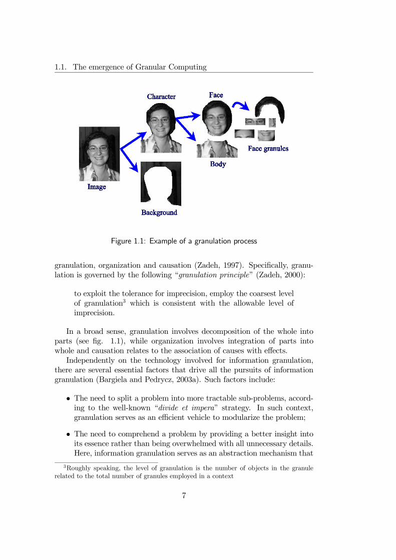
Figure 1.1: Example of a granulation process
granulation, organization and causation (Zadeh, 1997). Specifically, granu-lation is governed by the following “granulation principle” (Zadeh, 2000):
to exploit the tolerance for imprecision, employ the coarsest levelof granulation3 which is consistent with the allowable level ofimprecision.
In a broad sense, granulation involves decomposition of the whole intoparts (see fig. 1.1), while organization involves integration of parts intowhole and causation relates to the association of causes with effects.Independently on the technology involved for information granulation,
there are several essential factors that drive all the pursuits of informationgranulation (Bargiela and Pedrycz, 2003a). Such factors include:
• The need to split a problem into more tractable sub-problems, accord-ing to the well-known “divide et impera” strategy. In such context,granulation serves as an efficient vehicle to modularize the problem;
• The need to comprehend a problem by providing a better insight intoits essence rather than being overwhelmed with all unnecessary details.Here, information granulation serves as an abstraction mechanism that
3Roughly speaking, the level of granulation is the number of objects in the granulerelated to the total number of granules employed in a context
7
Chapter 1. Granular Computing
hides unnecessary information. By changing the level of granularity, itis possible to hide or reveal details according to the required specificityduring a certain design phase;
• The need for processing information in a human-centric modality. Ac-tually, information granules do not exist as tangible physical entitiesbut they are conceptual entities that emerge from information as adirect consequence of the continuous quest for abstraction, summariza-tion and condensation of information by human beings.
The process of information granulation and the nature of informationgranules imply the definition of a formalism that is well-suited to representthe problem at hand. There are a number of formal frameworks in whichinformation granules can be defined. Such frameworks are well-known andthoroughly investigated both from a theoretical and applicative standpoint.A short list of such frameworks, which includes the most common used withinGranular Computing, is the following:
• Set Theory and Interval Analysis (Bargiela, 2001; Hansen, 1975;Jaulin et al., 2001; Kearfott and Kreinovich, 1996; Moore, 1962; Morse,1965; Sunaga, 1958; Warmus, 1956)
• Fuzzy Set Theory (Dubois and Prade, 1980; Dubois and Prade, 1997;Kandel, 1982; Klir and Folger, 1988; Klir, 2001; Pedrycz and Gomide,1998; Zadeh, 1965; Zadeh, 1975a; Zadeh, 1975b; Zadeh, 1978; Zimmer-mann, 2001)
• Rough Set Theory (Lin and Cercone, 1997; Pal and Skowron, 1999;Pawlak, 1982; Pawlak, 1999; Nguyen and Skowron, 2001)
• Probabilistic (Random) Set Theory (Butz and Lingras, 2004;Cressie, 1993; Matheron, 1975; Stoyan et al., 1995; Zadeh, 2002; Zadeh,2003)
• Dempster-Shafer Belief Theory (Dempster, 1966; Dubois and Prade,1992; Fagin and Halpern, 1989; Klir and Ramer, 1990; Nguyen, 1978;Ruspini et al., 1992; Shafer, 1976; Shafer, 1987)
• etc.
8

1.2. Theory of Fuzzy Information Granulation
1.2 Theory of Fuzzy Information Granulation
Among all formal frameworks for Granular Computing, Fuzzy Set Theoryhas undoubtedly a prominent position4. The key feature of Fuzzy Set Theorystands in the possibility of formally express concepts of continuous bound-aries. Such blurred concepts are at the core of human perception processes,which often end up with linguistic terms belonging to natural language. It isevident that while these concepts are useful in the context of a certain prob-lem, as well as convenient in any communication realized in natural language,their set-based formal model will lead to serious representation drawbacks.Such “epistemic divide” between concepts and their formalization is primarilydue to the vagueness property of conceptual representations, as well-pointedby Russel (Russell, 1923):
[...] Vagueness and precision alike are characteristics which canonly belong to a representation, of which language is an example.They have to do with the relation between a representation andthat which it represents. Apart from representation, whethercognitive or mechanical, there can be no such thing as vaguenessor precision; things are what they are, and there is an end ofit. [...] law of excluded middle is true when precise symbols areemployed, but it is not true when symbols are vague, as, in fact,all symbols are. [...] All traditional logic habitually assumes thatprecise symbols are being employed. It is therefore not applicableto this terrestrial life, but only to an imagined celestial existence.
Vagueness cannot be removed from human cognition, as already pointedout by the philosopher Arthur Schopenhauer (1788—1860), whose positioncould be synthesized with the words of Tarrazo (Tarrazo, 2004):
we work with (symbolic) representations of ourselves, our envi-ronment, and the events we notice; these representations are ap-proximate at best because we simply do not know enough; whatmatters to us is to make better decisions using these subjec-tive representations. We employ those representations to solveimportant problems, which are unfailingly interdisciplinary andforward-looking. Anything interdisciplinary is bound to be only
4Granular Computing is often subsumed by Fuzzy Set Theory, especially in the con-text of Computational Intelligence and Soft Computing. However, it is thought that adistinction of the two terms acknowledges the credits of all non-fuzzy, yet granular-based,frameworks.
9
Chapter 1. Granular Computing
imperfectly represented. Further, the problems we must addressare important (e.g. career decisions, house purchases, retirementfinancing, etc.) because their effects are often felt substantiallyand during many years into the future. Very importantly, ourstrategies to deal with them must be played out in a shiftingfuture where many elements can only be approximated.
Fuzzy Sets are the contribution of Lotfi Zadeh (Zadeh, 1965). They can beconceived as generalizations of ordinary sets that admit partial membershipof elements. Based on such extended assumption, Fuzzy Set Theory — and thecorresponding Fuzzy Logic — has been formalized in several ways (Bellmanand Giertz, 1973; Goguen, 1967; Gottwald, 1979; Hájek, 1998; Mendel andJohn, 2002; Novák et al., 1999; Ramot et al., 2002). In the simplest setting, afuzzy set is described by a membership function, which maps the elements ofa Universe of Discourse U into the unit interval [0, 1]. Membership functionsquantify the notion of partial membership and define the semantics of a fuzzyset. Dubois and Prade (Dubois and Prade, 1997) discussed three points ofinterpretation of fuzzy set semantics:
Similarity The membership value of an element of the Universe of Discourseis interpreted as a degree of proximity to a prototype element. Thisis an interpretation that is particularly useful in the field of PatternRecognition (Bellman et al., 1966). This is also an appropriate inter-pretation in the context of Granular Computing, since information canbe granulated based on the similarity of object to some prototypes.
Preference A fuzzy set represent a granule of more or less preferred objectsand the membership values indicate their respective degree of desider-ability, or — in a decision making context — the degree of feasibility(Saaty, 1980). This point of view is deeply rooted in the realm ofdecision analysis with approximate reasoning.
Uncertainty The membership value determines the degree of possibilitythat some variable assumes a certain value. The values encompassedby the support of the fuzzy sets are mutually exclusive and the mem-bership grades rank these values in terms of their plausibility (Zadeh,1978). Possibility can have either a physical or an epistemic mean-ing. The physical meaning of possibility is related to the concept offeasibility, while its epistemic meaning is associated to the degree of“unsurprisingness” (Dubois and Prade, 1988).
From their introduction, fuzzy sets gained numerous achievements, es-pecially in applicative frameworks. According to Zadeh, fuzzy sets gained
10

1.2. Theory of Fuzzy Information Granulation
success because they ‹‹exploit the tolerance for imprecision and uncertaintyto achieve tractability, robustness, and low solution cost›› (Zadeh, 1994).Fuzzy Set Theory is not the only theoretical framework that allows suchkind of exploitation: actually several methodologies are inspired to the tol-erance for imprecision and uncertainty, and they fall in the wider field ofSoft Computing5. However, the key feature of Fuzzy Set Theory stands inthe possibility of giving a formal and procedural representation of linguisticterms used to express human-centered concepts (Ostasiewicz, 1999). Thisfacet is in line with the basic principles of Granular Computing and it ledto the development of the Theory of Fuzzy Information Granulation, whoseprincipal aim is to give a mathematical foundation to model the cognitivetasks of humans in granulating information and reason with it (Zadeh, 1997).
1.2.1 Granulation as a cognitive task
Within the Theory of Fuzzy Information Granulation, a special emphasisis given to the cognitive tasks of granulation (intended as dividing a wholeinto parts) and fuzzification, that replaces a crisp set with a fuzzy set. Thecombination of granulation and fuzzification (called “f.g-granulation” or “f.g-generalization”) leads to the basic concept of linguistic variable, fuzzy ruleset and fuzzy graph.The necessity for f.g-generalization is given by several motivations, in-
cluding:
1. Unavailability of precise (i.e. crisp or fine-grained) information. Thisoccurs in everyday decision making, as well as economic systems, etc.
2. High cost for precise information, e.g. in diagnostic systems, qualitycontrol, decision analysis, etc.
3. Unnecessity of precise information. This occurs in most human activi-ties, like parking, cooking, art crafting, etc.
4. Low-cost systems, like consumer or throw-away products, where thetrade-off between quality and cost is critical.
The Theory of Fuzzy Information Granulation is based on the conceptof generalized constraint, according to which an information granule for-mally represents an elastic constraint on the possible values of a modelled
5The terms “Soft Computing” and “Computational Intelligence” assumed over theyears a convergent meaning, so that it is common nowadays to refer to both terms assynonyms.
11
Chapter 1. Granular Computing
attribute. This theory provides a basis for Computing with Words, which isa methodology where words are used in place of numbers for computing andreasoning. Fuzzy Sets plays a pivotal role in Computing with Words in thesense that words are viewed as labels of fuzzy granules, which in turn modelsoft constraints on physical variables (Zadeh, 1996a). The inferential ma-chinery that enables information processing within Computing with Wordsis the Approximate Reasoning, which is accomplished by means of the un-derlying Fuzzy Set Theory (Yager, 1999). Computing with Words providesa powerful tool for human-centric — yet automated — information processing.It allows the setting of a highly interpretable knowledge base as well as ahighly transparent inference process, thus capturing the transparency bene-fits of symbolic processing without the inferential rigidity of classical expertsystems. The Theory of Fuzzy Information Granulation and Computing withWords shed new lights in classical Artificial Intelligence issues, as exemplifiedby the Precisiated Natural Language and Semiotical Cognitive InformationProcessing for natural language processing and understanding (Rieger, 2003;Zadeh, 2004).The Theory of Fuzzy Information Granulation can be also cast into the
realm of Cognitive Science, whose objectives include the understanding ofcognition and intelligence (Rapaport, 2003). In such context, the Theory ofFuzzy Information Granulation appears as a promising conceptual tool tobridge the historical gap between the “Physical Symbol System Hypothesis”— which states that cognition can be understood as symbolical sequentialcomputations that use mental representation as data (Fodor, 1975) — andthe connectionist approach, according to which intelligence and cognitionemerge from a system with an appropriate organized complexity, withoutbeing necessarily coded into symbols (Knight, 1990). The Theory of FuzzyInformation Granulation offers a double layer of knowledge representation:a first, symbolic layer of linguistic terms eventually structured within knowl-edge representation schemes, like fuzzy rule, fuzzy graphs, etc.; and a nu-merical level for expressing the semantics of the linguistic terms, which canemerge from perception-based sub-systems (such as neural networks) and canmanipulated by means of Approximate Reasoning.
1.2.2 Symbolic representation of fuzzy information gran-ules
The key advantage of a symbolically represented knowledge is the possibilityof communicating it among agents. Communication can have a continuous ordiscrete (analog) nature. Usually, analog communication is used to express
12
1.2. Theory of Fuzzy Information Granulation
emotive information among natural agents. Music, visive arts, but also odors,voice tones and animal sounds are all forms of analog communications. How-ever, communication of knowledge is always discrete and symbolical6. Thereasons behind the discrete nature of knowledge communication are the samethe justify the overwhelming success of digital computers over the analog de-vices: simplicity and reliability.As a discrete process, knowledge communication needs a language of sym-
bols to exist. Generally speaking, a language can be regarded as a systemconsisting of a representation (symbols) along with metaphor and some kindof grammar. Metaphor is a relation between representation and semanticsand is implicitly shared among all communicating actors. If a metaphor isnot shared among actors, communication cannot take place. As an exam-ple, the word (symbol) Tall, in the context of human heights, has a sharedmetaphor among all English-literate people and hence can be used in knowl-edge communication; on the other hand, the word Axdrw cannot be usedin communication until its meaning is fully specified.For the purposes of this study, knowledge communication can be catego-
rized according to the type of actors involved. A first type of communicationtakes place when all actors are human. Here, natural language is almostalways used7, which is often integrated with analog emotive forms of com-munications (facial expressions, tones, gestures, etc.). Natural language isvery rich, but it is ambiguous, imprecise and has a strong pragmatic compo-nent that is hard to model in any computational paradigm. It is neverthelessthe language that allowed the evolution of Science until the present days,even if in the last two centuries it has been strongly supported by mathe-matics. Nevertheless, the strict precision of the mathematical formalism hasbeen challenged in recent years by the development of alternative scientificapproaches, like qualitative modelling (IEE, 1988; Kuipers, 1994).The knowledge objects exchanged in a natural language communication
are sentences made of linguistic labels. Such labels denote real-world objectsby a composite cognitive task of perception and speech. Perception is under-stood as a process of translating sensory stimulation into an organized expe-rience. Though the perceptual process cannot be directly observed, relations
6It is interesting to note that communication of knowledge involves a process of recog-nition of symbolical structures from analog media. Examples of such process are therecognition of an electric/magnetic state of a digital medium as well as the recognitionof utterances, words or gestures. All such processes are different forms of informationgranulation.
7With exception to mathematical communication, where a formal language is preferred.However, it is very common that mathematical communication is enriched with severalnatural language notes to help understanding the involved concepts.
13

Chapter 1. Granular Computing
Concepts
Labels Objects
Denotation
Classification
Designation
Speech
Intension
Reference
Perception
Figure 1.2: Basic epistemic relationships between labels, concepts and objects
can be found between the various type of stimulation and their associatedexperiences or concepts8. The latter are complex constructions of simple ele-ments joined through association and are basic for human experience, whichhowever, is of organized wholes rater than collections of elements. In fig. 1.2,the relationships between linguistic labels, objects and concepts are depicted.Such relations correspond to a cognitive task, and include other importanttasks such as denotation, reference, intension and classification. This model,introduced in (Toth, 1999) highlights the prominent importance of the per-ception task within human cognition.According to H. Toth (Toth, 1997), fuzziness is a property of perceptions,
i.e. concepts originated from perceptive tasks. Perceptions, as vaguely de-fined entities, stand opposite to measurement-based objects, which are thebasic knowledge granules of classical Science. However, even though classicalScience has led to brilliant successes during time, it failed to solve problemsin which humans are mostly adequate. Agile robots, text summarization,
8Strictly speaking, perception is a cognitive process whose results are called percepts.However, since there is not a uniform terminology in literature, hereafter the term “per-ception” will be used to indicate both the process and the results. The latter will also bedenoted as “concepts”.
14

1.2. Theory of Fuzzy Information Granulation
language translation, car driving, etc. are only few examples of problemsthat are not — and maybe cannot be — solved by measurement-based sci-ence. Based on such consideration, novel perspectives can be envisioned thattake perceptions as central objects for scientific exploitation (Barsalou, 1999;Zadeh, 2000).Opposite to human communication is communication among computers.
In the most usual case, a formal language is adopted so as to avoid anypossible information loss due to the adoption of imprecise languages. Thiscommon choice is motivated by the necessity of exact information processingthat can replace humans in the most tedious and mechanical tasks. Such for-mal languages are inherently measurement-based and are specifically suitedfor symbolic information processing. However, with the advent of intelligentagents that act in complex environments, precise knowledge communicationhas been challenged and novel research directions, like “communication be-tween granular worlds”, have been opened (Bargiela and Pedrycz, 2003a).When communication involves both humans and computers, two signif-
icant distinctions must be made, depending on the direction of communi-cation. In the case of human-to-computer communication, the languagesused are almost always formal in order to avoid ambiguity and indetermi-nacy in computer information processing. Most of such kind of languagesare universal, i.e. they can express anything (or almost anything) thatcan be computable in the Turing sense. The distinction between all suchlanguages stands in the specific purposes the language is design for (e.g.programming languages, query languages, declarative languages, etc.). Theprincipal metaphors of such languages are usually simple, well-defined andmeasurement-based. For example, the metaphors of a declarative program-ming language are: predicates, terms and connectives.In the classical case, perceptions can be communicated to computers in
forms of facts and predicates, but their meaning must be exhaustively spec-ified with a huge corpus of axioms and statements that — apart from trivialcases — only approximate the real significance of the perceptions. As a con-sequence of the simple metaphors involved in such formal languages, thecomputer does not understand the meaning of perceptions but can derivefacts based on syntactical derivation rules. Such possibility of reasoningand acting based only on formal manipulation of symbols is at the centerof the philosophical debate on the possibility of a real intelligence in com-puter systems (Dreyfus and Dreyfus, 1986; Searle, 1980). Furthermore, mostcomputer languages do not support vagueness in representing information,thus disabling any possibility of representing perceptions in a human-centeredfashion. In such a situation, Granular Computing, and especially the Theoryof Fuzzy Information Granulation with derived paradigms like Precisiated
15
Chapter 1. Granular Computing
Natural Language, promise to be effective tools for humans to communicateperception-based information also to computer systems.When computers communicate knowledge to humans, they can use sev-
eral means. Usually, text-based communication provides for measurementsand precise information (conditions, states, facts, etc.), while graphical —and multimedia — communication easily conveys perception-based informa-tion. For example, charts provide graphical objects that are perceived byhumans to form judgements, which could be subsequently used to take de-cisions. Intuitive communication of information is a research issue withinthe field of Human-Computer Interaction (Raskin, 1994; Shneiderman andPlaisant, 2004). However, it should be observed that computers still maintainmeasurement-based information, which is rendered in visual form to stimu-late perceptions by humans; as a consequence, computers still cannot performperception-based reasoning and actions. An interesting question concernsthe possibility for computers of dealing with perception-based informationboth for reasoning and communication. The Theory of Fuzzy InformationGranulation provides a way for representing perception-based information,and Computing with Words — along with the Logic of Perception — enablesreasoning and communication of perception-based knowledge. However, suchtheories and methodologies do not tackle the problem of learning perception-based knowledge, or stated differently, forming information granules fromdata.
1.2.3 Interpretability of fuzzy information granules
The automatic generation of information granules from data is an extremelyimportant task, since it gives to machines the ability of adapting their be-havior dynamically. Granules generation (or extraction) can be accomplishedthrough the application of learning techniques especially suited for the formalframwork in which information granules are defined.Within the Theory of Fuzzy Information Granulation, the extraction of
information granules can be achieved through learning techniques that ac-quire fuzzy sets from data. Learning techniques that make use of FuzzySet Theory are numerous and embrace several approaches. Fuzzy Clustering(Baraldi and Blonda, 1999), Fuzzy Decision Trees (Janikow, 1998), FuzzyClassifiers (Kuncheva, 2000), Fuzzy Cognitive Maps (Kosko, 1986), Neuro-Fuzzy Networks (Nauck et al., 1997), etc. are just few examples of methodsand models that are aimed to acquire knowledge from data defined by meansof fuzzy sets. It could be stated that almost all learning techniques classi-cally belonging to Machine Learning, Explorative Data Analysis and DataMining have been adapted to acquire knowledge represented by fuzzy sets or
16

1.2. Theory of Fuzzy Information Granulation
fuzzy relations. Furthermore, the existence of universal approximation mod-els based on Fuzzy Set Theory has been proved (Wang, 1992). However, suchmodels and techniques do not take into account the perceptive nature of theacquired knowledge. The communication of such knowledge to a human usermust be carried out only by means of a formal language, which associatesarbitrary symbols to fuzzy sets and provides for each of them a functionalform to represent their semantics. This language for communication is veryfar from natural language, where symbols carry a meaning ipso facto, on thebasis of an implicit metaphor shared by the actors of the communication.As a consequence of the language gap, communication of the knowledge ac-quired by adaptive models can be only made by means of measurements (e.g.the parameters of the fuzzy membership functions), thus losing the potentialbenefits of a perception-based framework for reasoning and communicating.To obtain perception-based models, the learning algorithms used to ac-
quire knowledge from data must yield fuzzy information granules that canbe naturally labelled by linguistic terms, i.e. symbols that belong to thenatural language. The attachment of such terms to fuzzy sets must be doneby taking into account the metaphor carried by each linguistic term. Asan example, the linguistic term Tall can be assigned to a fuzzy set onlyif its semantics actually embraces the class of heights that people perceiveas tall (provided a tolerance for the vague definition off “being tall”) anddoes not include (or includes with low membership) heights that people donot perceive as tall. Information granules that can be attached to a linguis-tic term are called interpretable information granules, and models based oninterpretable information granules are called interpretable fuzzy models.In literature, the term interpretability is often assimilated as a synony-
mous of transparency, so that the two words are used interchangeably. Inaddition, in the attempt to give a distinct definition of the two terms, someconfusion exists. As an example, in (Riid and Rüstern, 2003) the definitionsof transparency and interpretability are exchanged w.r.t. definitions given in(Johansson et al., 2004)9. The two terms actually refer to two distinct prop-erties of models. Hereafter, the term “transparency” is meant to refer to aninherent property of a model whose behavior can be explained in terms of itscomponents and their relations. On the other hand, a model is interpretableif its behavior is intelligible, i.e. it can be easily perceived and understood bya user. Transparency is a metamathematical concept10 while interpretabil-ity has a more cognitive aspect and its study permeates several disciplines,including Machine Learning (IJCAI, 1995). Based on such definitions, fuzzy
9Here, the term comptrehensibility is used instead of interpretability10Transparency can be related with “white-box” models
17
Chapter 1. Granular Computing
models can be considered inherently transparent, because their behavior isclearly explained in terms of the involved information granules and the in-ference process, but their interpretability cannot be guaranteed until furtherinsights are made.Interpretability in Fuzzy Information Granulation is an intuitive prop-
erty, because it deals with the association of fuzzy information granules —which are mathematical entities — with metaphorical symbols (the linguisticterms), which conversely belong to the blurry realm of human linguistics.As a consequence, research on interpretable information granules and inter-pretable fuzzy models does not lead to a unique direction. Furthermore,interpretability issues have been investigated only in recent years since for-merly accuracy was the main concern of fuzzy modelling.Interpretability issues in fuzzy modelling has been tackled in several ways,
including two main approaches. A first approach concerns the complexityreduction of the knowledge structure, by balancing the trade-off betweenaccuracy and simplicity. The strategy of reducing the complexity of theknowledge structure is coherent to the notorious Occam Razor’s Principle11,which is restated in Information Theory as the Minimum Description Lengthprinciple (Rissanen, 1978). Complexity reduction can be achieved by re-ducing the dimensionality of the problem, e.g. by feature selection (Cordónet al., 2003; Tikk et al., 2003; Vanhoucke and Silipo, 2003), while featureextraction (e.g. Principal Component Analysis) is not recommended be-cause the extracted features do not have any physical — hence interpretable— meaning. Other methods to reduce complexity include the selection of anappropriate level of granularity of the knowledge base (Cordón et al., 2003;Guillaume and Charnomordic, 2003), the fusion of similar information gran-ules (Espinosa and Vandewalle, 2003; Abonyi et al., 2003; Sudkamp et al.,2003), elimination of low-relevant information granules (Baranyi et al., 2003;Setnes, 2003), and hierarchical structuring of the knowledge base (Tikk andBaranyi, 2003a).The Minimum Description Length principle has been effectively adopted
in Artificial Intelligence for inductive learning of hypotheses (Gao et al.,2000). However, in interpretable fuzzy modelling it could be insufficient toguarantee interpretable information granules since labelling with linguisticterms could be still hard if further properties, other than simplicity, are notsatisfied. Based on such consideration, some authors propose the adoptionof several constraints that are imposed on the knowledge based and on the
11‹‹Pluralitas non est ponenda sine neccesitate››, which translates literally into Englishas “Plurality should not be posited without necessity”. Occam’s Razor is nowadays usuallystated as “of two equivalent theories or explanations, all other things being equal, thesimpler one is to be preferred”
18
1.2. Theory of Fuzzy Information Granulation
model to achieve interpretability. These interpretability constraints actuallydefine the mathematical characterization of the notion of interpretability.Several authors propose a constraint-oriented approach to interpretable fuzzymodelling, including the pioneering works of de Oliveira (Valente de Oliveira,1999b) and Chow et al. (Chow et al., 1999).Interpretability constraints force the process of information granulation
to (totally or partially) satisfy a set of properties that are judged neces-sary to allow the attachment of linguistic labels to the information granulesconstituting the knowledge base. A preliminary survey of methods to pro-tect interpretability in fuzzy modelling is given in (Guillaume, 2001; Casillaset al., 2003). Constrained information granulation of data can be achievedin several ways, which can be roughly grouped in three main categories
Regularized learning The learning algorithms are aimed to extract infor-mation granules so as to optimize an objective function that promotesthe definition of an accurate knowledge base but penalizes those solu-tions that violate interpretability constraints. The objective functionmust be encoded in an appropriate way so as to be applied to clas-sical constrained optimization techniques (e.g. Lagrangian multipliersmethod).
Genetic algorithms Information granules are properly encoded into a pop-ulation of individuals that evolve according to an evolutionary cycle,which involves a selection process that fosters the survival of accurateand interpretable information granules. Genetic algorithms are espe-cially useful when the interpretability constraints cannot be formalizedas simple mathematical functions that can be optimized according toclassical optimization techniques (e.g. gradient descent, least squaremethods, etc.). Moreover, the multi-objective genetic algorithms arecapable to deal with several objective functions simultaneously (e.g.one objective function that evaluates accuracy and another to assessinterpretability). However, the drawback of genetic algorithms is theirinherent inefficiency that restricts their applicability.
Ad-hoc algorithms Interpretable information granules are extracted ac-cording to learning algorithms that encode interpretability constraintswithin the extraction procedure. Such type of algorithms are usuallymore efficient than others but, due to their variable design, are difficultto develop.
Scientific investigation in interpretable information granulation is stillopen. Despite the numerous techniques for interpretable fuzzy modelling,
19

Chapter 1. Granular Computing
there in no agreement on a definitive set of constraints that characterizeinterpretability. As a consequence, different sets of constraints are proposed,which involve the definition of methods and technique that are sometimesincomparable. Such disagreement is due to the blurry nature of the notion ofinterpretability, which is subjective and in some cases application oriented.Moreover, each single interpretability constraint can have a psychologicalsupport, a common sense justification or even it has no justifications at all.For such reason, a comprehensive study of all interpretability constraintsproposed in literature would lead to a number of benefits, including:
• An homogenous description, which helps the selection of interpretabil-ity constraints for specific applicative purposes;
• The identification of potential different notions of interpretability, re-lated to the nature of the information granules (e.g. information gran-ules describing quantities vs. those describing qualities);
• A critical review of interpretability constraints, which may help to dis-card those constraints that are not strongly justified by objective orexperimental supports, or to subsume different constraints in more gen-eralized ones, from which novel properties may emerge;
• A common notation, which helps the encoding of different interpretabil-ity constraints within the same framework or algorithm;
• The possibility of identifying newmethods for interpretable informationgranulation.
In the next Chapter, interpretability constraints known in literature aredeeply surveyed with a homogeneous mathematical formalization and criti-cally reviewed from several perspectives encompassing computational, psy-chological, and linguistic considerations.
20

Chapter 2
Interpretability Constraints forFuzzy Information Granules
2.1 Introduction
The aim of this Chapter is to deeply survey the mathematical characteriza-tion of the intuitive notion of interpretability within the context of the Theoryof Fuzzy Information Granulation. The survey is the result of a systematicinsight of scientific works concerning interpretable fuzzy modelling.A common approach used to define interpretability involves the definition
of a set of constraints to be verified on information granules. Unfortunately,there is not a set of constraints universally accepted to characterize the no-tion of interpretability. On the contrary, every author adopts a customizedset of interpretability constraints. Such variability is due to the subjectivejudgement motivating the inclusion of each single constraint in the attemptto formalize interpretability. Indeed, while some constraints are psycholog-ically motivated (also with experimental support), others are justified onlyby common sense or are application-specific. As a consequence, the choiceof including a formal constraint in defining interpretability could depend onsubjective decision. To achieve a better agreement on which constraints arestrictly necessary to define interpretability and which are more superfluous,an analytical systematization of all formal constraints could be a valid help.In this Chapter, interpretability constraints are analytically described by
providing, for each one, a formal definition — where possible — and a jus-tification of its use in interpretable fuzzy modelling. As the number of in-terpretability constraints is quite high, they have been classified accordingto several categories. The chosen taxonomy is only one of several possiblecategorizations. As an example, in (Peña-Reyes and Sipper, 2003) a divi-
21

Chapter 2. Interpretability Constraints for Fuzzy Information Granules
sion between “syntactic” and “semantic” constraints can be found. Sincethis work is aimed in analyzing interpretability within the context of Gran-ular Computing, a different taxonomy has been preferred. Following therepresentation of fuzzy information granules as linguistically labelled multi-dimensional fuzzy sets, the following taxonomy of interpretability constraintshas been used:
• Constraints for (one-dimensional) fuzzy sets;• Constraints for frames of cognition, i.e. families of one-dimensionalfuzzy sets defined on the same Universe of Discourse;
• Constraints for fuzzy information granules;• Constraints for fuzzy rules;• Constraints for fuzzy models;• Constraints for learning algorithms;The last three categories of constraints have been included because the
most frequent use of fuzzy information granules is within rule-based fuzzymodels, which are often equipped with learning capabilities to refine theirpredictive accuracy.In the following, interpretability constraints are described according to
the aforementioned taxonomy. It should be noted that some constraints havea rigid mathematical definition, while others have a more fuzzy description.Such variability of formulations should not be considered negatively but asa direct consequence of the inherent blurriness of the “interpretability” con-cept.
2.2 Constraints on Fuzzy sets
The first level of interpretability analysis concerns each fuzzy set involved inthe representation of an information granule. In order to be labelled by asemantically sound linguistic term, each fuzzy set must be shaped so as tosatisfy some requirements justified by common sense.Hereafter, a fuzzy set is A is fully defined by its membership function1
µA defined as:
µA : U → [0, 1] (2.1)
1Note that on the semantic level, the symbols A and µA denote the same object.However the use of two symbols helps to distinguish the variable A from its value µA
22

2.2. Constraints on Fuzzy sets
where the domain U of the membership function is called Universe of Dis-course and includes all admissible values that may belong to a fuzzy set. Theset of all possible fuzzy sets definable on U is denoted with F (U).Before introducing interpretability constraints, some considerations about
the Universe of Discourse U are noteworthy. In this work, it is assumed thatU is a closed interval of the real line. Such definition has some importantconsequences:
1. The Universe of Discourse is numerical and real2. The choice of numer-ical universe is necessary when physical systems have to be representedby fuzzy models, though categorical universes may be chosen when it isnecessary to represent more abstract data types (e.g. conceptual cate-gories). For fuzzy sets defined on categorical universes, however, manyinterpretability constraints are not applicable while other constraints— though formally applicable — loose significance. Real numbers areadopted because they generalize natural and rational numbers. Theadjoint value of including all real elements instead of only rational onesstands in facilitating model analysis, which is often accomplished withmathematical Calculus. More structured domains, such as complexnumbers or mathematical/symbolical structures are more applicationspecific and hence are not included in interpretability analysis.
2. The Universe of the Discourse is one-dimensional, hence fuzzy setsmodel single attributes of a complex system and composite attributesare represented by more complex information granules. Unidimension-ality is often required in interpretable fuzzy modelling and is implicitlyassumed by most authors in the field (Babuška, 1999; Ishibuchi andYamamoto, 2002; Setnes et al., 1998b). Unidimensional fuzzy sets helpto better understand complex systems in terms of composite relations(e.g. “sepal is Wide, petal is Long and color is Purple”),while they could be unable to model complex relations that can hardlybe represented in terms of composition of single attributes (e.g. howto represent the knowledge that “john is Nice” in terms of eyes’color, nose dimension, etc.?). This latter form of knowledge is “non-representable”3 and hence it is out of scope for interpretable fuzzy in-
2i.e. subset of the real line3The representability of knowledge is a long disputed theme in Cognitive Science. From
the strong assumptions of the Representational Theory of Mind (Fodor, 1975), several ar-guments have been arisen so much to deny the representational nature of human knowledgein favour of emergent phenomena (Norman, 1981). More recent developments try to re-late and fruitfully exploit both points of view and hybrid systems (such as neuro-fuzzynetworks) are concrete realizations of this new school of thougth.
23
Chapter 2. Interpretability Constraints for Fuzzy Information Granules
formation granulation. In such case, black box models, such as neuralnetworks, are more suitable.
3. As a closed interval, the Universe of Discourse has an infimum mU =inf U and a supremum MU = supU and all numbers between the twoextreme values are legitimate elements of the Universe. This definitionof Universe of Discourse simplifies modelling and is not particularlylimiting when representing physical attributes, which are almost al-ways expressible as values in a range. In quantitative modelling, eithermU or MU may be infinite. In such cases, interpretability analysismust be adapted to enable infinite support domains4. In other con-texts, many authors assume the Universe of Discourse to be the unitaryinterval [0, 1] or [−1, 1]. This restriction is useful when elements of dif-ferent Universes of Discourse appear in the same computation (e.g. inclustering algorithms) to avoid problems due to different scales. Suchrescaling is obviously not limiting since it is always possible to find bi-jective mappings that transform these specific intervals in any requiredclosed interval, being it limited or not. However, this mapping mayhamper the physical meaning of the attribute, so the rescaling shouldbe limited only within the processing steps that require it, and theoriginal universe of discourse must be resorted when knowledge has tobe represented in an interpretable form.
In the following, a number of interpretability constraints are defined anddescribed. Such constraints apply to each fuzzy set singularly, which is as-sumed to be characterized by a membership function defined over a Universeof Discourse U defined as a limited closed interval [mU ,MU ] ⊂ R.
Normality
Constraint 1 A fuzzy set A must be normal, i.e. there exists at least oneelement (called prototype) with full membership:
∃x ∈ U : µA (x) = 1 (2.2)
A fuzzy set is sub-normal if it is not normal. In fig. 2.1, normality andsub-normality are graphically depicted for two fuzzy sets. The normality
4The adaptation of interpretability analysis to infinite support domains is straightfor-ward in most cases, but may require adjoint mathematical burden that does not conveyuseful information in analyzing the key interpretability issues of fuzzy information granu-lation. For such reason, in this work the Universe of discourse is assumed to be limited,i.e. MU < +∞ and mU > −∞.
24
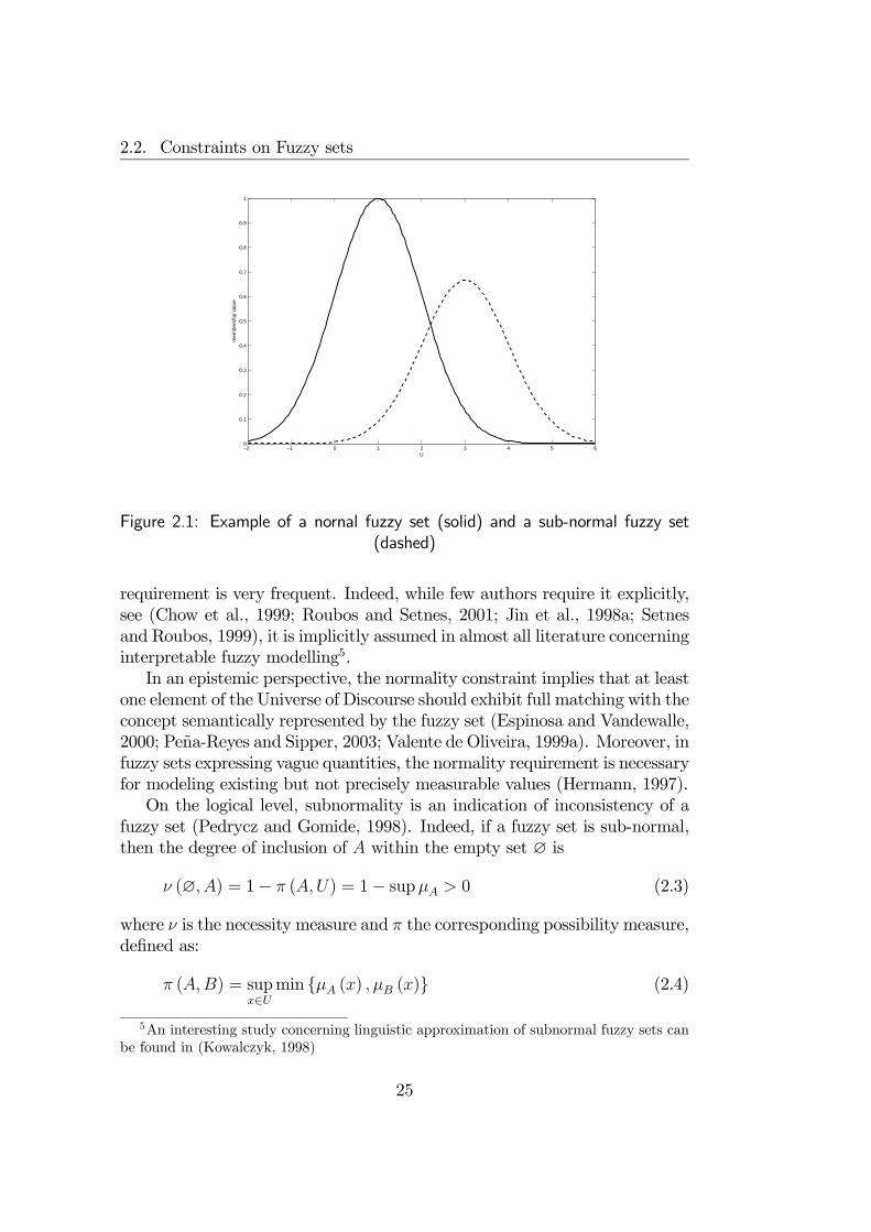
2.2. Constraints on Fuzzy sets
−2 −1 0 1 2 3 4 5 60
0.1
0.2
0.3
0.4
0.5
0.6
0.7
0.8
0.9
1
U
mem
bers
hip
valu
e
Figure 2.1: Example of a nornal fuzzy set (solid) and a sub-normal fuzzy set(dashed)
requirement is very frequent. Indeed, while few authors require it explicitly,see (Chow et al., 1999; Roubos and Setnes, 2001; Jin et al., 1998a; Setnesand Roubos, 1999), it is implicitly assumed in almost all literature concerninginterpretable fuzzy modelling5.In an epistemic perspective, the normality constraint implies that at least
one element of the Universe of Discourse should exhibit full matching with theconcept semantically represented by the fuzzy set (Espinosa and Vandewalle,2000; Peña-Reyes and Sipper, 2003; Valente de Oliveira, 1999a). Moreover, infuzzy sets expressing vague quantities, the normality requirement is necessaryfor modeling existing but not precisely measurable values (Hermann, 1997).On the logical level, subnormality is an indication of inconsistency of a
fuzzy set (Pedrycz and Gomide, 1998). Indeed, if a fuzzy set is sub-normal,then the degree of inclusion of A within the empty set ∅ is
ν (∅, A) = 1− π (A,U) = 1− supµA > 0 (2.3)
where ν is the necessity measure and π the corresponding possibility measure,defined as:
π (A,B) = supx∈U
min µA (x) , µB (x) (2.4)
5An interesting study concerning linguistic approximation of subnormal fuzzy sets canbe found in (Kowalczyk, 1998)
25

Chapter 2. Interpretability Constraints for Fuzzy Information Granules
Inconsistent fuzzy sets are problematic in inference systems because theymay produce unexpected and unsatisfactory results6. As a consequence,the normality constraint should be verified for all fuzzy sets involved in aknowledge-based model.
Convexity
Constraint 2 A fuzzy set A must be convex7 i.e. the membership values ofelements belonging to any interval are not lower than the membership valuesat the interval’s extremes:
∀a, b, x ∈ U : a ≤ x ≤ b→ µA (x) ≥ min µA (a) , µA (b) (2.5)
Alternatively, α-cuts may be used to define convexity:
∀α ∈ [0, 1]∃mα,Mα : [A]α = [mα,Mα] (2.6)
being each α-cut defined as:
[A]α = x ∈ U : µA (x) ≥ α (2.7)
The fuzzy set A is strictly convex if inequalities in (2.5) are strict, i.e.without equality signs.
Convexity is an important requirement that is often implicitly assumed ininterpretable fuzzy modelling (convexity is explicitly required in (Chow et al.,1999)). It can be considered as a completion of the normality requirement.Indeed, while normality constraints imposes that at least one element (aprototype) of the Universe of Discourse is fully represented by the fuzzy set,convexity assures that the concept represented by the fuzzy set graduallyloses its evidence as elements of fuzzy sets become far from the prototypes.In this way, the concept represented by the fuzzy set can be conceived aselementary, i.e. it is related to a single specific property of a perceived object(see fig. 2.2).Convexity is a defining property of fuzzy numbers and fuzzy vectors8.
A fuzzy number is a semantic representation of vague quantities labelled,e.g., with “About x” where x is a rational number. Fuzzy numbers can
6This could be viewed as a generalization of the pseudo-Scoto meta-theorem, whichstates that from a contradiction every formula (including its negation) can be derived.
7It should be remarked that the notion of convexity of fuzzy sets is different from thenotion of convexity of functions. Actually, convex fuzzy sets are often characterized bymembership functions that are not convex
8A fuzzy vector is a vector of fuzzy numbers
26
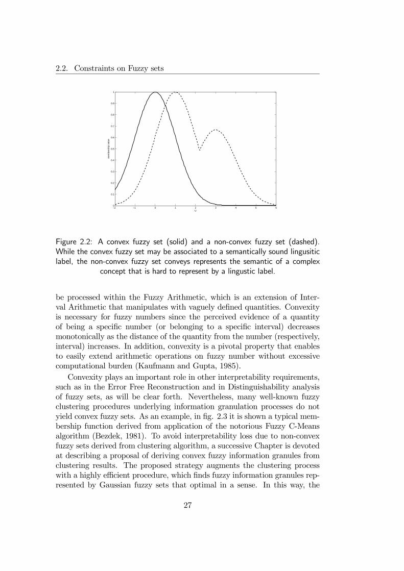
2.2. Constraints on Fuzzy sets
−2 −1 0 1 2 3 4 5 60
0.1
0.2
0.3
0.4
0.5
0.6
0.7
0.8
0.9
1
U
mem
bers
hip
valu
e
Figure 2.2: A convex fuzzy set (solid) and a non-convex fuzzy set (dashed).While the convex fuzzy set may be associated to a semantically sound lingusiticlabel, the non-convex fuzzy set conveys represents the semantic of a complex
concept that is hard to represent by a lingustic label.
be processed within the Fuzzy Arithmetic, which is an extension of Inter-val Arithmetic that manipulates with vaguely defined quantities. Convexityis necessary for fuzzy numbers since the perceived evidence of a quantityof being a specific number (or belonging to a specific interval) decreasesmonotonically as the distance of the quantity from the number (respectively,interval) increases. In addition, convexity is a pivotal property that enablesto easily extend arithmetic operations on fuzzy number without excessivecomputational burden (Kaufmann and Gupta, 1985).Convexity plays an important role in other interpretability requirements,
such as in the Error Free Reconstruction and in Distinguishability analysisof fuzzy sets, as will be clear forth. Nevertheless, many well-known fuzzyclustering procedures underlying information granulation processes do notyield convex fuzzy sets. As an example, in fig. 2.3 it is shown a typical mem-bership function derived from application of the notorious Fuzzy C-Meansalgorithm (Bezdek, 1981). To avoid interpretability loss due to non-convexfuzzy sets derived from clustering algorithm, a successive Chapter is devotedat describing a proposal of deriving convex fuzzy information granules fromclustering results. The proposed strategy augments the clustering processwith a highly efficient procedure, which finds fuzzy information granules rep-resented by Gaussian fuzzy sets that optimal in a sense. In this way, the
27
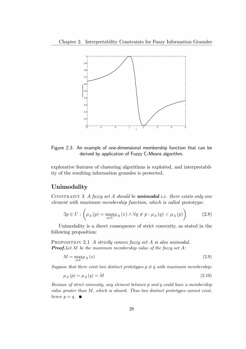
Chapter 2. Interpretability Constraints for Fuzzy Information Granules
−2 −1 0 1 2 3 4 50
0.1
0.2
0.3
0.4
0.5
0.6
0.7
0.8
0.9
1
U
mem
bers
hip
degr
ee
Figure 2.3: An example of one-dimensional membership function that can bederived by application of Fuzzy C-Means algorithm.
explorative features of clustering algorithms is exploited, and interpretabil-ity of the resulting information granules is protected.
Unimodality
Constraint 3 A fuzzy set A should be unimodal i.e. there exists only oneelement with maximum membership function, which is called prototype:
∃p ∈ U :
µµA (p) = max
x∈UµA (x) ∧ ∀q 6= p : µA (q) < µA (p)
¶(2.8)
Unimodality is a direct consequence of strict convexity, as stated in thefollowing proposition:
Proposition 2.1 A strictly convex fuzzy set A is also unimodal.Proof.Let M be the maximum membership value of the fuzzy set A:
M = maxxeU
µA (x) (2.9)
Suppose that there exist two distinct prototypes p 6= q with maximum membership:
µA (p) = µA (q) =M (2.10)
Because of strict convexity, any element between p and q could have a membershipvalue greater than M , which is absurd. Thus two distinct prototypes cannot exist,hence p = q.
28
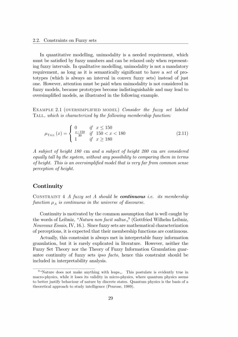
2.2. Constraints on Fuzzy sets
In quantitative modelling, unimodality is a needed requirement, whichmust be satisfied by fuzzy numbers and can be relaxed only when represent-ing fuzzy intervals. In qualitative modelling, unimodality is not a mandatoryrequirement, as long as it is semantically significant to have a set of pro-totypes (which is always an interval in convex fuzzy sets) instead of justone. However, attention must be paid when unimodality is not considered infuzzy models, because prototypes become indistinguishable and may lead tooversimplified models, as illustrated in the following example.
Example 2.1 (oversimplified model) Consider the fuzzy set labeledTall, which is characterized by the following membership function:
µTall (x) =
0 if x ≤ 150x−15030
if 150 < x < 1801 if x ≥ 180
(2.11)
A subject of height 180 cm and a subject of height 200 cm are consideredequally tall by the system, without any possibility to comparing them in termsof height. This is an oversimplified model that is very far from common senseperception of height.
Continuity
Constraint 4 A fuzzy set A should be continuous i.e. its membershipfunction µA is continuous in the universe of discourse.
Continuity is motivated by the common assumption that is well caught bythe words of Leibniz, “Natura non facit saltus„9 (Gottfried Wilhelm Leibniz,Nouveaux Essais, IV, 16.). Since fuzzy sets are mathematical characterizationof perceptions, it is expected that their membership functions are continuous.Actually, this constraint is always met in interpretable fuzzy information
granulation, but it is rarely explicated in literature. However, neither theFuzzy Set Theory nor the Theory of Fuzzy Information Granulation guar-antee continuity of fuzzy sets ipso facto, hence this constraint should beincluded in interpretability analysis.
9“Nature does not make anything with leaps„. This postulate is evidently true inmacro-physics, while it loses its validity in micro-physics, where quantum physics seemsto better justify behaviour of nature by discrete states. Quantum physics is the basis of atheoretical approach to study intelligence (Penrose, 1989).
29
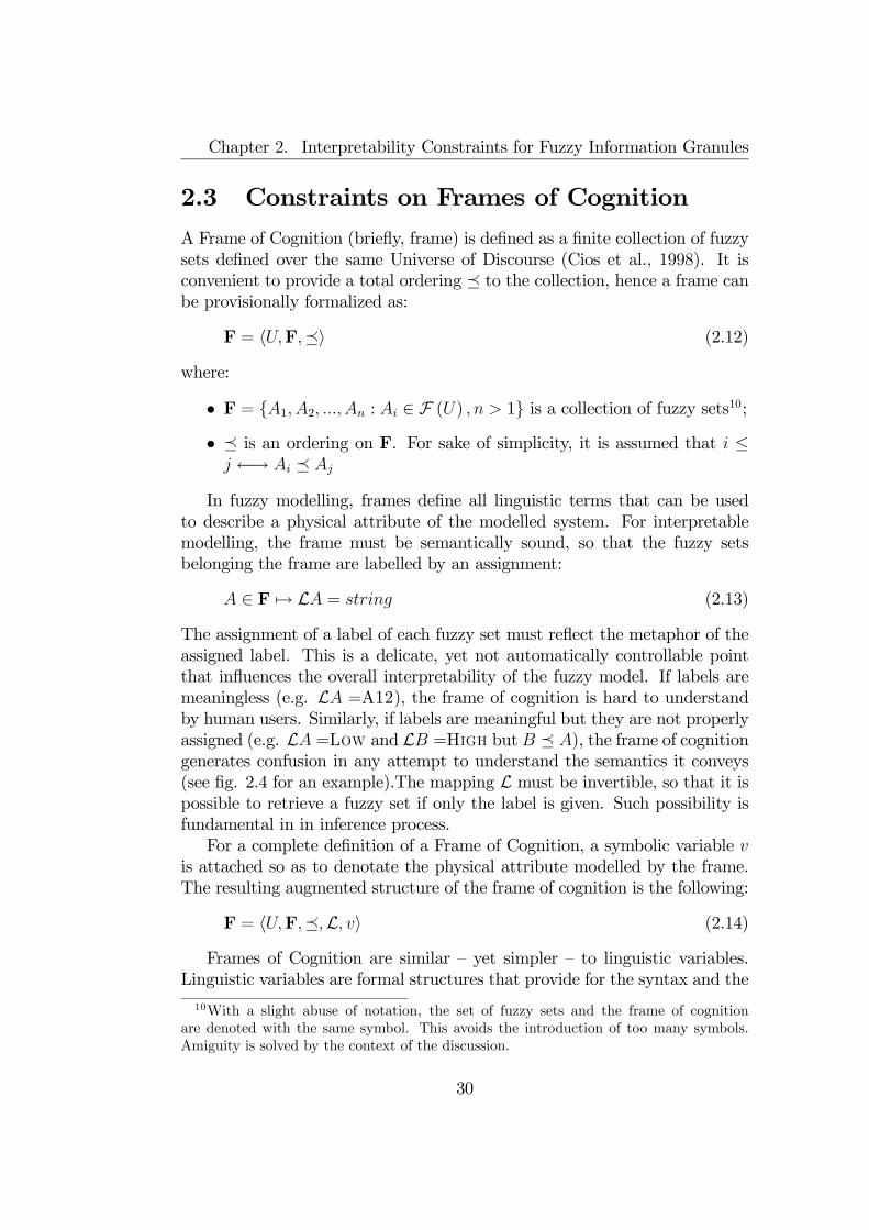
Chapter 2. Interpretability Constraints for Fuzzy Information Granules
2.3 Constraints on Frames of Cognition
A Frame of Cognition (briefly, frame) is defined as a finite collection of fuzzysets defined over the same Universe of Discourse (Cios et al., 1998). It isconvenient to provide a total ordering ¹ to the collection, hence a frame canbe provisionally formalized as:
F = hU,F,¹i (2.12)
where:
• F = A1, A2, ..., An : Ai ∈ F (U) , n > 1 is a collection of fuzzy sets10;• ¹ is an ordering on F. For sake of simplicity, it is assumed that i ≤j ←→ Ai ¹ Aj
In fuzzy modelling, frames define all linguistic terms that can be usedto describe a physical attribute of the modelled system. For interpretablemodelling, the frame must be semantically sound, so that the fuzzy setsbelonging the frame are labelled by an assignment:
A ∈ F 7→ LA = string (2.13)
The assignment of a label of each fuzzy set must reflect the metaphor of theassigned label. This is a delicate, yet not automatically controllable pointthat influences the overall interpretability of the fuzzy model. If labels aremeaningless (e.g. LA =A12), the frame of cognition is hard to understandby human users. Similarly, if labels are meaningful but they are not properlyassigned (e.g. LA =Low and LB =High but B ¹ A), the frame of cognitiongenerates confusion in any attempt to understand the semantics it conveys(see fig. 2.4 for an example).The mapping L must be invertible, so that it ispossible to retrieve a fuzzy set if only the label is given. Such possibility isfundamental in in inference process.For a complete definition of a Frame of Cognition, a symbolic variable v
is attached so as to denotate the physical attribute modelled by the frame.The resulting augmented structure of the frame of cognition is the following:
F = hU,F,¹,L, vi (2.14)
Frames of Cognition are similar — yet simpler — to linguistic variables.Linguistic variables are formal structures that provide for the syntax and the10With a slight abuse of notation, the set of fuzzy sets and the frame of cognition
are denoted with the same symbol. This avoids the introduction of too many symbols.Amiguity is solved by the context of the discussion.
30
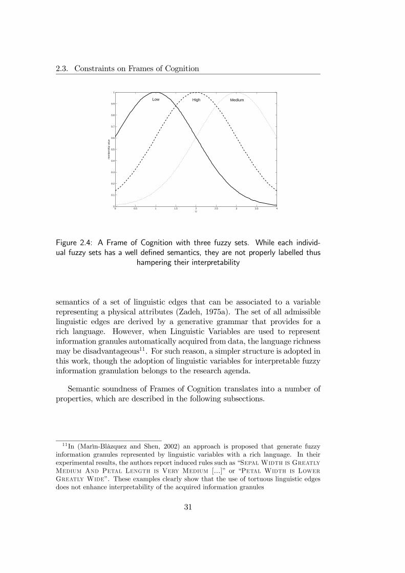
2.3. Constraints on Frames of Cognition
0 0.5 1 1.5 2 2.5 3 3.5 40
0.1
0.2
0.3
0.4
0.5
0.6
0.7
0.8
0.9
1
U
mem
bers
hip
valu
e
Low High Medium
Figure 2.4: A Frame of Cognition with three fuzzy sets. While each individ-ual fuzzy sets has a well defined semantics, they are not properly labelled thus
hampering their interpretability
semantics of a set of linguistic edges that can be associated to a variablerepresenting a physical attributes (Zadeh, 1975a). The set of all admissiblelinguistic edges are derived by a generative grammar that provides for arich language. However, when Linguistic Variables are used to representinformation granules automatically acquired from data, the language richnessmay be disadvantageous11. For such reason, a simpler structure is adopted inthis work, though the adoption of linguistic variables for interpretable fuzzyinformation granulation belongs to the research agenda.
Semantic soundness of Frames of Cognition translates into a number ofproperties, which are described in the following subsections.
11In (Marìn-Blàzquez and Shen, 2002) an approach is proposed that generate fuzzyinformation granules represented by linguistic variables with a rich language. In theirexperimental results, the authors report induced rules such as “Sepal Width is GreatlyMedium And Petal Length is Very Medium [...]” or “Petal Width is LowerGreatly Wide”. These examples clearly show that the use of tortuous linguistic edgesdoes not enhance interpretability of the acquired information granules
31
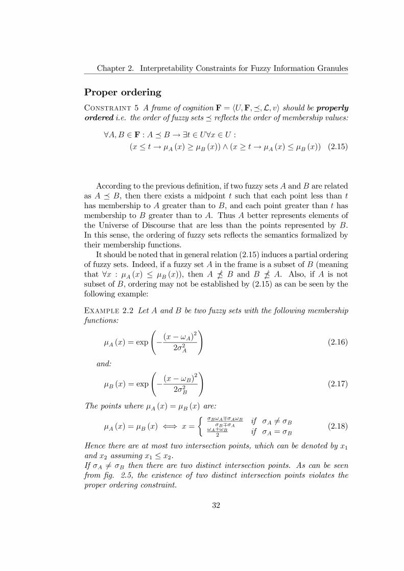
Chapter 2. Interpretability Constraints for Fuzzy Information Granules
Proper ordering
Constraint 5 A frame of cognition F = hU,F,¹,L, vi should be properlyordered i.e. the order of fuzzy sets ¹ reflects the order of membership values:
∀A,B ∈ F : A ¹ B → ∃t ∈ U∀x ∈ U :
(x ≤ t→ µA (x) ≥ µB (x)) ∧ (x ≥ t→ µA (x) ≤ µB (x)) (2.15)
According to the previous definition, if two fuzzy sets A and B are relatedas A ¹ B, then there exists a midpoint t such that each point less than thas membership to A greater than to B, and each point greater than t hasmembership to B greater than to A. Thus A better represents elements ofthe Universe of Discourse that are less than the points represented by B.In this sense, the ordering of fuzzy sets reflects the semantics formalized bytheir membership functions.It should be noted that in general relation (2.15) induces a partial ordering
of fuzzy sets. Indeed, if a fuzzy set A in the frame is a subset of B (meaningthat ∀x : µA (x) ≤ µB (x)), then A ± B and B ± A. Also, if A is notsubset of B, ordering may not be established by (2.15) as can be seen by thefollowing example:
Example 2.2 Let A and B be two fuzzy sets with the following membershipfunctions:
µA (x) = exp
Ã−(x− ωA)
2
2σ2A
!(2.16)
and:
µB (x) = exp
Ã−(x− ωB)
2
2σ2B
!(2.17)
The points where µA (x) = µB (x) are:
µA (x) = µB (x) ⇐⇒ x =
½ σBωA∓σAωBσB∓σA if σA 6= σB
ωA+ωB2
if σA = σB(2.18)
Hence there are at most two intersection points, which can be denoted by x1and x2 assuming x1 ≤ x2.If σA 6= σB then there are two distinct intersection points. As can be seenfrom fig. 2.5, the existence of two distinct intersection points violates theproper ordering constraint.
32

2.3. Constraints on Frames of Cognition
−2 −1 0 1 2 3 40
0.1
0.2
0.3
0.4
0.5
0.6
0.7
0.8
0.9
1
from thispoint properordering is violated
Figure 2.5: An example of violation of proper ordering
From the previous example, it could be observed that if ωA ≤ ωB, thenA and B could be considered ordered in some sense (e.g. if A and B rep-resent the fuzzy numbers ‘About ωA’ and ‘About ωB’, then A and B areintuitively ordered as A ¹ B). This weaker kind of order can be formalizedwith the following weaker condition:
Constraint 6 A frame of cognition F = hU,F,¹,L, vi should be weaklyproperly ordered i.e. the order of fuzzy sets ¹ reflects the order of proto-types:
∀A,B ∈ F : A ¹ B ⇔ min coreA ≤ min coreB (2.19)
where coreA = argmaxµA.
This new definition is weaker than that in (2.15) , in the sense thatit may not reflect the intuitive idea of ordering in some special cases (e.g.when one fuzzy set is subset of another fuzzy set). However, for normal,unimodal and convex fuzzy sets, weakly proper ordering can be consideredas an adequate constraint for interpretability analysis. In summary, weaklyproper ordering can be considered as a valid constraint for frames consistingof normal, unimodal and convex fuzzy sets, while (strict) proper ordering canbe assured when using specific shapes for fuzzy sets (e.g. isotope12 Gaussianfuzzy sets).
12Two Gaussian fuzzy sets are isotope if they have the same width. In such case, theinterection point between the two fuzzy sets is unique
33

Chapter 2. Interpretability Constraints for Fuzzy Information Granules
Justifiable number of elements
Constraint 7 The number of fuzzy sets in the frame should not be too high,preferably less than 7± 2This criterion is motivated by a psychological experiment reported in
(Miller, 1956) and considered in a number of papers concerning interpretablefuzzy modelling, e.g. in (Espinosa and Vandewalle, 2000; Jamei et al., 2001;Jiménez et al., 2001; Jin, 2000; Meesad and Yen, 2002; Valente de Oliveira,1999a; Paiva and Dourado, 2001; Peña-Reyes and Sipper, 2003; Setnes et al.,1998a). In his test battery, Miller proved that the span of absolute judg-ment13 and the span of immediate memory14 impose a severe limitation onthe amount of information that a human being is able to perceive, processand remember. Experimentally, the author found that the number of en-tities that can be clearly remembered for a short time is around 7, plus orminus 2, depending on the subject under examination. Interestingly, andquite surprisingly from a cognitive standpoint, complex information can bementally organized into unitary chunks of information that are treated assingle entities. In this way, the human brain is capable of perceive, processor remember in its short term memory both simple perceptions (e.g. tones)or more complex entities (e.g. faces), provided that the number of entities isless than “the magical number seven, plus or minus two„.The transposition of such important psychological result into interpretabil-
ity analysis leads to the criterion of reducing the number of fuzzy sets in aFrame of Cognition to a justifiable number of elements (see fig. 2.6). It alsogives a scientific explanation of the commonly adopted criterion of reducingthe complexity of a fuzzy model to make it more interpretable. Moreover,the criterion can be applied also to other element constituting a fuzzy model,e.g. the number of attributes (for the entire model or for each informationgranule) and the number of information granules. However, the psycholog-ically imposed limit of elements can be surpassed when it is necessary todefine more accurate models, which may require a greater number of ele-ments (fuzzy sets, attributes or rules) to describe the behavior of a system.
Distinguishability
Constraint 8 Any fuzzy set in the Frame of Cognition must be well dis-tinguishable from the remaining fuzzy sets of the frame
13Absolute judgment is the task of assigning numbers to stimuli of different perceivedmagnitudes. An example of absolute judgment is the assignment to different numbers toacustic impulses based on perceived tones.14The number of events that are reminded in the short term.
34

2.3. Constraints on Frames of Cognition
1 1.5 2 2.5 3 3.5 4 4.5 50
0.10.20.30.40.50.60.70.80.9
1
(a)
1 1.5 2 2.5 3 3.5 4 4.5 50
0.10.20.30.40.50.60.70.80.9
1
(b)
Figure 2.6: Example of Frame of Cognition with a five fuzzy sets (a) and anotherwith ten fuzzy sets (b). The association of liguistic labels to fuzzy sets of the
first frame is clearly easier than ti fuzzy sets of the second frame
Distinguishability is one of the most common interpretability constraintsadopted in fuzzy modelling literature (Babuška, 1999; Chow et al., 1999;Espinosa and Vandewalle, 2000; Guillaume and Charnomordic, 2004; Jameiet al., 2001; Jiménez et al., 2001; Jin and Sendhoff, 2003; Meesad and Yen,2002; Nauck and Kruse, 1998; Valente de Oliveira, 1999a; Paiva and Dourado,2001; Peña-Reyes and Sipper, 2003; Roubos and Setnes, 2001; Setnes et al.,1998a).Formally, Distinguishability is a relation between fuzzy sets defined on
the same Universe of Discourse. Roughly speaking, distinguishable fuzzysets are well disjunct so they represent distinct concepts and can be assignedto semantically different linguistic labels. Well distinguishable fuzzy setsprovide the following advantages in fuzzy modelling:
• Obviate the subjective establishment of membership-function/linguisticterm association (Valente de Oliveira, 1998);
• Avoids potential inconsistencies in fuzzy models (Valente de Oliveira,1999b);
• Reduce model’s redundancy and consequently computational complex-ity (Setnes et al., 1998a);
35
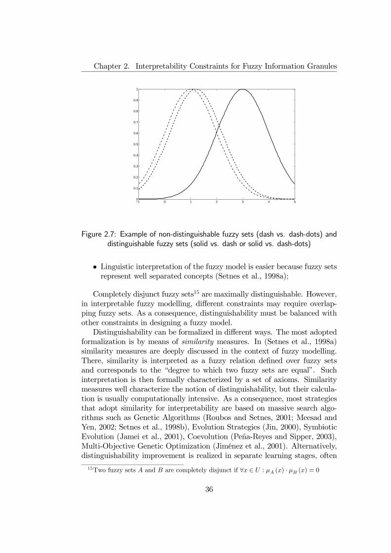
Chapter 2. Interpretability Constraints for Fuzzy Information Granules
−1 0 1 2 3 4 50
0.1
0.2
0.3
0.4
0.5
0.6
0.7
0.8
0.9
1
Figure 2.7: Example of non-distinguishable fuzzy sets (dash vs. dash-dots) anddistinguishable fuzzy sets (solid vs. dash or solid vs. dash-dots)
• Linguistic interpretation of the fuzzy model is easier because fuzzy setsrepresent well separated concepts (Setnes et al., 1998a);
Completely disjunct fuzzy sets15 are maximally distinguishable. However,in interpretable fuzzy modelling, different constraints may require overlap-ping fuzzy sets. As a consequence, distinguishability must be balanced withother constraints in designing a fuzzy model.Distinguishability can be formalized in different ways. The most adopted
formalization is by means of similarity measures. In (Setnes et al., 1998a)similarity measures are deeply discussed in the context of fuzzy modelling.There, similarity is interpreted as a fuzzy relation defined over fuzzy setsand corresponds to the “degree to which two fuzzy sets are equal”. Suchinterpretation is then formally characterized by a set of axioms. Similaritymeasures well characterize the notion of distinguishability, but their calcula-tion is usually computationally intensive. As a consequence, most strategiesthat adopt similarity for interpretability are based on massive search algo-rithms such as Genetic Algorithms (Roubos and Setnes, 2001; Meesad andYen, 2002; Setnes et al., 1998b), Evolution Strategies (Jin, 2000), SymbioticEvolution (Jamei et al., 2001), Coevolution (Peña-Reyes and Sipper, 2003),Multi-Objective Genetic Optimization (Jiménez et al., 2001). Alternatively,distinguishability improvement is realized in separate learning stages, often
15Two fuzzy sets A and B are completely disjunct if ∀x ∈ U : µA (x) · µB (x) = 0
36
2.3. Constraints on Frames of Cognition
after some data driven procedure like clustering, in which similar fuzzy setsare usually merged together (Paiva and Dourado, 2001; Setnes et al., 1998a).When distinguishability constraint must be included in less time consum-
ing learning procedures, like in neural learning, similarity measures are nolonger used. In (Paiva and Dourado, 2001), after a merging stage that usessimilarity, fine tuning is achieved by simply imposing some heuristic con-straints on centers and width of membership functions. In (Jin and Send-hoff, 2003), a distance function between fuzzy sets (restricted to the Gaussianshape) is used in the regularization part of the RBF cost function. In (Guil-laume and Charnomordic, 2004) a sophisticated distance function is used tomerge fuzzy sets. In (Nauck and Kruse, 1998; Espinosa and Vandewalle,2000; Castellano et al., 2002) the possibility measure is adopted to evaluatedistinguishability.The possibility measure has some attracting features that promote a
deeper investigation in the context of distinguishability assessment. Al-though it is not a similarity measure, it has a clear and well-establishedsemantics since it can be interpreted as the degree to which the flexibleconstraint “X isA” is satisfied (Zadeh, 1978). Moreover, the possibility mea-sure between fuzzy sets can be often analytically defined in terms of fuzzysets’ parameters. This makes possibility evaluation very efficient, thus allow-ing the employment of this measure in computationally inexpensive learningschemes. For this reason, a successive Chapter is devoted to a discussion con-cerning the theoretical justification of the adoption of the possibility measurein the context of distinguishability analysis.
Completeness (coverage)
Constraint 9 A Frame of Cognition F must be complete i.e. each ele-ment of the Universe of Discourse U belongs at least to one fuzzy set of theFrame of Cognition:
∀x ∈ U∃A ∈ F : µA (x) > 0 (2.20)
A more general definition of the completeness constraint is given in (Jang,1992):
Constraint 10 A Frame of Cognition F is α−complete if each elementof the Universe of Discourse U belongs at least to one fuzzy set of the framewith membership not lower than α:
∀x ∈ U∃A ∈ F : µA (x) ≥ α (2.21)
37

Chapter 2. Interpretability Constraints for Fuzzy Information Granules
−1 0 1 2 3 4 50
0.1
0.2
0.3
0.4
0.5
0.6
0.7
0.8
0.9
1
Figure 2.8: Example of completeness violation. In the highlighted regions of theUniverse of Discourse (ellipses) 0.5-completeness is not verified.
Completeness is a property of deductive systems that has been used in thecontext of Artificial Intelligence to indicate that the knowledge representationscheme can represent every entity within the intended domain (Valente deOliveira, 1999b). When applied to fuzzy models, completeness states thatthe fuzzy model should be able to infer a proper conclusion for every in-put (Lee and Lee, 1975). Hermann (Hermann, 1997) justifies completeness(there called ‘cover full range’) by the fact that in human reasoning therewill never be a gap of description within the range of the variable. On thecontrary, incompleteness may be a consequence of model adaption from dataand can be considered a symptom of overfitting (Jin et al., 1999). Gener-ally, α−completeness is preferable in interpretable fuzzy modelling, becauseit assures that each element of the Universe of Discourse is well representedby the frame of cognition, i.e. each element possess a property (representedby a fuzzy set) with a minimum degree α (see also fig. 2.8).In an attempt to assess α−completeness (and α−incompleteness), in
(Meesad and Yen, 2002) the following measure is proposed (here adaptedto continuous Universe of Discourse):
CDα =
Rx∈U :max
X∈FµX(x)>α
dxRUdx
(2.22)
IDα = 1− CDα (2.23)
38
2.3. Constraints on Frames of Cognition
Incompleteness Degree (IDα) is hence the complementary of the Complete-ness Degree (CDα). These to measures, which take values in the range [0, 1],can be effectively used in genetic optimization process in order to maximizecompleteness while improving the accuracy of the model. When interpretabil-ity is of major concern, however, techniques must be adopted so that thecompleteness criterion is always fulfilled (i.e. CDα = 1 for a given α).When using triangular fuzzy sets, 0.5-completeness is easy to guarantee
by a proper placement of fuzzy sets parameters (Espinosa and Vandewalle,2000; Guillaume and Charnomordic, 2004; Kruse et al., 1994). More specif-ically, given two triangular fuzzy sets of membership functions T [a1, b1, c1]and T [a2, b2, c2], where:
T [a, b, c] (x) = max
½0,min
½x− a
b− a,x− c
b− c
¾¾(2.24)
0.5-completeness in the interval [b1, b2] is guaranteed if b1 < b2 and:
a2 = b1 ∧ b2 = c1 (2.25)
Indeed, with such constraints on the parameters the membership func-tions can be simplified as:
∀x ∈ [b1, b2] :½
T [a1, b1, c1] (x) =x−c1b1−c1
T [a1, b1, c1] (x) = T [b1, c1, c2] (x) =x−b1c1−b1
(2.26)
Hence, if T [a1, b1, c1] (x) ≤ 0.5, then:
x− b1c1 − b1
≤ 12=⇒ −x ≥ −c1 + b1
2=⇒
T [a1, b1, c1] (x) =x− c1b1 − c1
≥ 1
2(2.27)
From this result, a useful theorem can be settled:
Proposition 2.2 Let a Frame of Cognition F = hU,F,¹,L, vi with
F = A1, A2, ..., An : Ai ¹ Ai+1 (2.28)
be defined an the Universe of Discourse U = [mU ,MU ] and assume thateach fuzzy set Ai is triangular with membership function T [ai, bi, ci] suchthat ai+1 = bi, bi+1 = ci and b1 = a1 = mU and bn = cn = MU . Then,0.5−completeness in the sense of 2.21 is verified.
39
Chapter 2. Interpretability Constraints for Fuzzy Information Granules
Proof.As previously observed, each couple of consecutive fuzzy set guarantees0.5-coverage in the interval [bi, bi+1]. Since:
U =n−1[i=1
[bi, bi+1] (2.29)
completeness is verified in the entire Universe of Discourse.The results on triangular fuzzy sets can be easily extended to trapezoidal
fuzzy sets by taking care of the interval of prototypes that belong to theircore. When using Gaussian fuzzy sets, coverage can be guaranteed by properconstraints on the parameters of the membership functions, as described inthe following proposition.
Proposition 2.3 Let a Frame of Cognition hU,F,¹,L, vi withF = A1, A2, ..., An : Ai ¹ Ai+1 (2.30)
be defined on the Universe of Discourse U = [mU ,MU ] and assume that eachfuzzy set Ai is Gaussian with membership function G [ωi, σi] defined as:
µAi (x) = G [ωi, σi] (x) = exp
Ã−(x− ωi)
2
2σ2i
!(2.31)
Let t1, t2, ..., tn−1 a sequence of points such that mU < t1 < t2 < ... < tn−1 <MU and let t0 = 2mU−t1 and tn = 2MU−tn−1. If the centers and the widthsof the membership functions in (2.31) are such that:
ωi =ti−1 + ti2
(2.32)
and:
σi =ti − ti−1
2√−2 lnα (2.33)
then α−completeness in the sense of 2.21 is verified.Proof.The membership values of ti to the fuzzy sets Ai and Ai+1 are the following:
µAi (ti) = exp
−³ti − ti−1+ti
2
´22³
ti−ti−12√−2 lnα
´2 = exp lnα = α (2.34)
µAi+1 (ti) = exp
−³ti − ti+ti+1
2
´22³
ti+1−ti2√−2 lnα
´2 = exp lnα = α (2.35)
40

2.3. Constraints on Frames of Cognition
Hence, ti is the intersection point of the two fuzzy sets Ai and Ai+1. Since Gaussianfuzzy sets are strictly convex, then:
∀x ∈ [ωi, ti] : µAi(x) ≥ α (2.36)
∀x ∈ [ti, ωi+1] : µAi+1(x) ≥ α (2.37)
As a consequence, in each interval [ωi, ωi+1] α−completeness is verified. Moreover,since ω1 = (t0 + t1) /2 = mU and ωn = (tn−1 + tn) /2 = MU , it follows thatU = [ω1, ω2]∪ [ω2, ω3]∪ · · · [ωn−1, ωn] hence α−completeness is verified in all theUniverse of Discourse.
In (Valente de Oliveira, 1999a) a more general criterion is given to guaran-tee α−completeness. The criterion states that for all elements of the Universeof Discourse, the sigma-count (Kosko, 1992) of all membership values mustbe greater than α:
∀x ∈ U : p
sXX∈F
µpX (x) ≥ α (2.38)
The authors claim that the proposed criterion can be applied to fuzzysets of any shape. However, no proof is provided to guarantee that constraint(2.38) guarantees α−completeness, without assuming specific shapes to fuzzysets. Indeed, it is trivial to find simple examples of frames of cognition where(2.38) is true but α−completeness is not assured:Example 2.3 Consider a frame of two fuzzy sets A and B such that thereexists an element of the universe of discourse where:
µA (x) = µB (x) =
√2
4(2.39)
Then, for p = 2:qµ2A (x) + µ2B (x) = 0.5 (2.40)
However, max µA (x) , µB (x) =√24< 0.5. Moreover, it can be easily proved
that for p ≤ 2, inequality (2.38) is verified but 0.5−completeness is not as-sured.
Example 2.4 In a more general settlement, consider a frame of two fuzzysets A and B such that there exists an element of the universe of discoursewhere:
µA (x) = µB (x) = β < α (2.41)
41
Chapter 2. Interpretability Constraints for Fuzzy Information Granules
Then, for a generic p ≥ 1:p
qµpA (x) + µpB (x) ≥ α←→ β ≥ α
21p
(2.42)
Since, for each p ≥ 1, 2 1p > 1, then it is always possible to find β such thatβ < α and inequality (2.38) is verified. Actually, it can be easily proved thatequivalence between (2.38) and (2.21) is verified only for p → +∞, since21p →p→∞
1.
The choice of the coverage level α is subjective and application specific.However, a value α ≥ 0.5 since preferable since in this way it is assured thateach element of U is well represented by at least one concept semanticallydefined by one fuzzy set of the frame16.
Complementarity (Σ1-criterion)
Constraint 11 For each element of the Universe of Discourse, all mem-bership values of the frame must sum up to one:
∀x ∈ U :XX∈F
µX (x) = 1 (2.43)
The Complementarity criterion assures that the Universe of Discourse isdivided into a Ruspini partition (Ruspini, 1969), also called Bezdek partition(see fig. 2.9 for an example).The adoption of Ruspini partitions is very common in fuzzy modelling
(especially in fuzzy clustering (Bezdek, 1981)) but it is controversial in in-terpretability analysis. In (Peña-Reyes and Sipper, 2003), the authors statethat complementarity “guarantees uniform distribution of meaning amongelement. However, such statement is unclear and does not shed light on anymotivation to adopt Ruspini partitions in interpretable fuzzy informationgranulation.Herrmann (Hermann, 1997) motivates complementarity with the follow-
ing properties, which are direct consequences of the adoption of a Ruspinipartition:
Full acceptance Whenever a membership value decreases from 1, anothervalue increases from zero:
∀x ∈ U∀A ∈ F∃B ∈ F\ A : µA (x) < 1→ µB (x) > 0 (2.44)
16In (Pedrycz and Gomide, 1998) it is also proved that the best crisp approximation ofa fuzzy set is its 0.5-cut. Thus, membership values greater than this treshold denote abetter evidence of the truth of the proposition semantically interpreted by a fuzzy set.
42

2.3. Constraints on Frames of Cognition
0 0.1 0.2 0.3 0.4 0.5 0.6 0.7 0.8 0.9 1
0
0.2
0.4
0.6
0.8
1
(a)
0 0.1 0.2 0.3 0.4 0.5 0.6 0.7 0.8 0.9 1
0
0.2
0.4
0.6
0.8
1
(b)
Figure 2.9: Example of two frames of cognition with complementarity constraintverified (a) and violated (b).
From a semantic perspective, full acceptance implies that when a con-cept does not fully represent an element, then there exists anotherconcept that (at least partially) represents the element.
Negations The negation of a fuzzy set is expressed as the sum of the re-maining membership values:
∀x ∈ U∀A ∈ F : µ¬A (x) =X
X∈F\A
µX (x) (2.45)
However, this property has not any explanation in terms of inter-pretability analysis, because the summation operator is not a t-conorm17.Moreover, negation in fuzzy modelling has a far more complex seman-tics, as pointed out in (Ferri et al., 1999). As a consequence, thisproperty can be considered as a only mere technical consequence of thecomplementarity criterion.
No three a time For any element of the Universe of Discourse, no morethan two fuzzy sets have non-zero membership degree:
∀x ∈ U : |X ∈ F : µX (x) > 0| ≤ 2 (2.46)
17A t-conorm is a diadic function that is used to define the semantics of the disjunctionlogical operator.
43

Chapter 2. Interpretability Constraints for Fuzzy Information Granules
This property is very important in the inference context, because itassures that the number of elements involved in the inference processis limited, thus economizing the resources (time and space) involved inthe inference. However, such property appears quite stringent in in-terpretability analysis, since it precludes that more than two conceptspartially represent the same element (e.g. if x is Low with high de-gree and Medium with small degree, it could also be expected that xcannot be also High, though with a small degree). Actually, limitedsupport fuzzy sets (e.g. triangular or trapezoidal) allow economic infer-ence without satisfying the property (2.46). Moreover, infinite supportfuzzy sets (e.g. Gaussian) can be used in efficient inference by discard-ing fuzzy sets whose membership degrees are lower than a threshold.Hence the property (2.46) does not appear significant in interpretabilityanalysis, nor in efficient inference processes.
The most significant contribution of complementarity to interpretabilityappears to be full acceptance, which can be also seen as a consequence of thecompleteness constraint. Furthermore, complementarity has been criticizedby some authors because it is not recognized that degrees of truth (or degreesof membership) have an additive nature. In some cases, fuzzy clustering algo-rithms based on Ruspini partitions have been directly related to probabilisticclustering schemes (Wang et al., 2004). In (Krishnapuram and Keller, 1993),Ruspini partitions have been considered as expressing a “degree of sharing„and possibilistic clustering has been proposed to better represent the intuitiveidea of cluster membership. From the above consideration, with the addi-tional difficulty of preserving complementarity in non-piecewise linear fuzzysets, complementarity does not appear as a valid constraint for interpretablefuzzy modelling.
Uniform granulation
Constraint 12 The cardinalities of all fuzzy sets18 of the frame must bealmost the same
∀A,B ∈ F : |A| ≈ |B| (2.47)
Uniform granulation is a criterion required in (Lotfi et al., 1996) as adiscriminating property for distinguishing understandable models — like thoseproposed in (Glorennec, 1993; Ishibuchi et al., 1994; Kong and Kosko, 1992) —
18The simplest definition of the cardinality of a fuzzy set is |A| = RUµA (x) dx. A deeper
discussion on fuzzy set cardinalities can be found in (Maciej, 2000).
44

2.3. Constraints on Frames of Cognition
−1 0 1 2 3 4 5 6 70
0.2
0.4
0.6
0.8
1
(a)
−1 0 1 2 3 4 5 6 70
0.2
0.4
0.6
0.8
1
(b)
Figure 2.10: Comparative example of two Frames of Congition where UniformGranulation is verified (a) and violated (b)
from those models where linguistic understandability is not of major concern,as in (Berenji and Khedkar, 1993; Sun, 1994). The criterion can be formalizedby fixing a class of membership functions (e.g. Gaussian) characterized bya set of parameters (e.g. center and width). Uniform granulation is thenformalized either by restricting the range of variability of such parameters(e.g. the width must vary only in a predefined range) or by assigning apenalty value depending on the actual values of each parameter, e.g.:
< (p) = 1
1 + exp (− (p− pmin) /σp)− 1
1 + exp ((p− pmax) /σp)(2.48)
where p is a parameter, pmin and pmax are the minimum/maximum valuesallowed for p and σp is the dispersion index. In fig. 2.10 a Frame of Cognitionwith Uniform Granulation is graphically compared with a frame that violatesthe constraint.While it is recognizable that uniform granulation appears as a desirable
property for interpretable fuzzy models, it should be noted that such con-straint is not often used in specialized literature. This can be motivated bythe necessity of specifying a high number of hyper-parameters (i.e. rangeof variability and the dispersion index), especially when fuzzy models mustbe acquired from data. An additional problem may arise when data to bemined for model induction have not a uniform distribution. In such a case,the uniform granulation may oppose to an accurate — yet understandable —
45
Chapter 2. Interpretability Constraints for Fuzzy Information Granules
description of data. Finally, it should be observed that human beings do notperceive stimuli with a uniform scale (e.g. the intensity of perceived sound islogarithmically related to the actual intensity of sound). Such nonlinearities,which translate into non uniformity of scales, should be taken into accountin interpretable fuzzy modelling.
Leftmost/Rightmost fuzzy sets
Constraint 13 The minimum (resp. maximum) element of the universeof discourse must be prototypes for some fuzzy set of the Frame of Cognition:
∃A,B ∈ F : µA (minU) = 1 ∧ µB (maxU) = 1 (2.49)
This constraint has been explicitly required in (Chow et al., 1999), butit is extensively used — without mention — in several works concerning inter-pretable fuzzy modelling. The constraints states that there exist two extremefuzzy sets that fully represent the limit values of the Universe of Discourse.An obvious consequence of frames that have leftmost/rightmost fuzzy setsand satisfy the weak proper ordering criterion (2.19) is that the leftmost fuzzyset is the first fuzzy set and the rightmost fuzzy set is the last, according tothe ordering relation ¹ specified within the frame. In fig. 2.11 an exampleof two Frames of Cognition, one verifying leftmost/rightmost fuzzy sets andthe other violating the constraint, is depicted.In a semiotic perspective, the constraint of leftmost/rightmost fuzzy sets
is extremely important because it could hamper the linguistic interpretabilityof the frame if violated. The following example illustrates the problem:
Example 2.5 Consider a frame of cognition of convex normal fuzzy sets,where the first fuzzy set (in the weakly properly order sense ), labelled asLow, has not its prototype in minU , i.e. µLow (minU) < 1. Since the fuzzyset is normal, there exists a prototype, which could be denoted as minU +ε, being ε > 0. Each element of the Universe of Discourse belonging to[minU,minU + ε[ has a degree of membership to the fuzzy set Low thatis lower than membership degree of element minU + ε. On a semiotic level,this means that elements in [minU,minU + ε[ have an evidence of “lowness”that is smaller than element minU + ε, but this opposes to the metaphoricalsemantic of the concept “being low”. This paradox can be solved by introduc-ing another fuzzy set, which may be labelled as Very Low, which has itsprototype in minU . In this way, the leftmost fuzzy set constraint is verified.
Leftmost/rightmost fuzzy sets are hence important in those frames thatexpress qualities on the Universe of Discourse (e.g. Low, Medium, High),
46

2.3. Constraints on Frames of Cognition
−1 (minU) 0 1 (minU+e) 2 3 4 5 6 7 0
0.10.20.30.40.50.60.70.80.9
1
(a)
−1 (minU) 0 1 2 3 4 5 6 7 0
0.10.20.30.40.50.60.70.80.9
1
(b)
Figure 2.11: Example of a Frame of Cognition violating leftmost/rightmost fuzzysets (a) and a frame veryfing such constraint (b).
so as to adhere to human intuition. However, such extreme fuzzy sets maynot exist in frames that express fuzzy quantities (e.g. about x, plus orminus y, etc.), since these labels do not convey any meaning of extremity.It is perhaps for this reason that many interpretable fuzzy information gran-ules, designed by fuzzy clustering techniques, do not have leftmost/rightmostmembership values. However, when results of fuzzy clustering are used todefine qualitatively labelled fuzzy sets, this constraint should be taken intoaccount.
Natural zero positioning
Constraint 14 If the number 0 belongs to the Universe of Discourse, itmust be prototype of a fuzzy set in the Frame of Cognition:
0 ∈ U → ∃A ∈ F : µA (0) = 1 (2.50)
This property states that the number 0, if included in the Universe ofDiscourse, should be fully represented by a fuzzy set of the Frame. Stateddifferently, this constraint specifies that the Frame must include a fuzzy setthat represents the concept “About 0” or similar. However, as stated bythe same authors that proposed this constraint, Natural Zero Positioningis a problem-specific constraint, especially useful in control problems (Va-lente de Oliveira, 1999a; Valente de Oliveira, 1999b). Generally speaking,
47

Chapter 2. Interpretability Constraints for Fuzzy Information Granules
natural zero positioning makes sense — and its application should be eval-uated — to Universes of Discourse of rational scale, i.e. sets where divisionbetween elements of the universe is a semantically correct operation (e.g.length/area/volume/weight measures lay on rational scales, but tempera-tures are not measured in rational scales).More interestingly, Natural Zero Positioning calls for a more general crite-
rion, which may be called “Natural S Positioning”, where S is a set of elementsin the Universe of Discourse which should be prototype of some fuzzy sets be-cause they have privileged semantics. The constraint of Leftmost/rightmostfuzzy sets falls in this more general criterion, having minU,maxU ⊆ S.Another example can be taken from the domain of accelerations, where thevalue 9.8m/ s2 (i.e. the gravitational acceleration) should be prototype of afuzzy set. In Celsius temperatures, both 0 C and 100 C may be consideredprototypes of two fuzzy sets, eventually labelled as IcingPoint and Boil-ingPoint respectively, if the frame is referred to water temperatures, whilethe value 37 C can be prototype for a fuzzy set if the frame refers to humanbody temperatures.
Error-free reconstruction
Constraint 15 Given a frame of cognition
F = A1, A2, . . . , An (2.51)
and a function
D: [0, 1]n → R (2.52)
each element of the Universe of the Discourse x must be perfectly recon-structed by applying the D to its membership degrees:
∀x ∈ U : D¡µA1 (x) , µA2 (x) , ..., µAn
(x)¢= x (2.53)
Error-free reconstruction guarantees that the ‘internal representation’ ofan element x of the Universe of Discourse — which is given by the sequenceof membership degrees µA1 (x) , . . . , µAn
(x) is a perfect representation of xw.r.t. the function D (Espinosa and Vandewalle, 2000; Valente de Oliveira,1999a). For interpretability analysis, this property is of great importancebecause it assures that the processing carried out by the model is coherentwith the measured value transformed by the frame, and different elementsshould lead to different processing tasks.Put more formally, error free reconstruction requires that the mapping
operated by the frame to the element must be invertible. In this sense,
48

2.4. Constraints on Fuzzy Information Granules
however, even if such mapping is actually invertible, a wrong choice of thefunction D may hide bijection. For such reason, in interpretability analysisa weaker form of error-free reconstruction appears more adequate:
Constraint 16 Given a frame of cognition
F = A1, A2, . . . , An (2.54)
there exists a function D: [0, 1]n → R such that each element of the Uni-verse of the Discourse x must be perfectly reconstructed by applying D to itsmembership degrees:
∃D : [0, 1]n → R,∀x ∈ U : D¡µA1 (x) , µA2 (x) , ..., µAn (x)
¢= x (2.55)
In fuzzy modelling, a dual problem should be also addressed, which con-cern the perfect reconstruction of the sequence of membership degrees whena single numerical value is given. This problem arises when the fuzzy modelprovides a single numerical value by means of a defuzzification procedureand one asks whether the defuzzified value is coherent with the member-ship degrees provided after processing. This is a far more complex problemthan that concerning error free reconstruction stated in (2.55) because itaddresses bijection of a mapping that transforms a multi-dimensional spaceinto a one-dimensional space.The issues related to error-free reconstruction are analyzed in the con-
text of fuzzy interfaces, which are frames of cognition analyzed in a purefunctional viewpoint, i.e. without explicitly addressing the interpretabilityissues. Nevertheless, theoretical results on fuzzy interfaces are of great im-portance in interpretability analysis. Theoretical issues on fuzzy interfacesare analyzed in a successive Chapter, which focus on characterizing the classof fuzzy sets that guarantee error-free reconstruction (in the weak sense),and provides theoretical results concerning the assessment of fuzzy interfacewhen error-free reconstruction is practically impossible.
2.4 Constraints on Fuzzy Information Gran-ules
A fuzzy information granule is defined as a linguistically labelled multidi-mensional fuzzy set. A convenient linguistic representation of an informationgranule is by means of soft-constraints, proposed by Zadeh in (Zadeh, 1997).In his original work, Zadeh proposed a general framework to represent infor-mation granules deriving from different paradigms, including the Theory of
49
Chapter 2. Interpretability Constraints for Fuzzy Information Granules
Probability or the Rough Sets Theory. Here, only the Fuzzy Set Theory isconsidered for representing information granules, which can be formalized asdescribed in the following.An atomic soft constraint is defined as a formal expression of the form:
v is FLv (2.56)
where v is a formal variable, “is” is a copula and FLv is a label associatedto a fuzzy set. Atomic soft constraints can be directly derived by a Frame ofCognition, which can be conveniently denoted as
Fv = hUv,Fv,¹v,Lv, vi (2.57)
provided that the label of the soft constraint is assigned to some fuzzy set ofthe frame:
∃A ∈ Fv : Lv (A) = FLv (2.58)
The semantics of a soft constraint is straightforward. The formal variableis evaluated according to an assignment function that associates the variablev to a fuzzy set in F (Uv) :
= (v) [x] = x ∈ F (Uv) (2.59)
In most cases, however, the evaluation of the variable maps to a singlenumerical value:
= (v) [x] = x (2.60)
The evaluation of the label FLv is achieved by retrieving the fuzzy setlabelled by FLv:
= (FLv) = L−1v (FLv) ∈ Fv (2.61)
Finally, the interpretation of the soft constraint “v is FLv”, denoted byFCv for convenience, is defined as
= (FCv) [x] = = (v is FLv) [x] = π¡L−1v (FLv) ,= (v) [x]
¢(2.62)
where π is the possibility function, defined as:
π (A,B) = sup minx∈Uv
µA (x) , µB (x) (2.63)
50
2.4. Constraints on Fuzzy Information Granules
Computation is simplified if the variable assignment associates a singlescalar value to the variable as in (2.60). In such a case the evaluation of afuzzy constraint reduces to:
= (FCv) [x] = µA (x) (2.64)
being
A = L−1v (FLv) (2.65)
More complex soft constraints can be composed by conjunction, disjunc-tion or negation of several atomic soft constraints, eventually defined in dif-ferent Universes of Discourse. In the most common case, conjunctive softconstraints are used, i.e. forms of the type
FCv1 and FCv2 and . . . and FCvnV(2.66)
The interpretation of such type of complex soft constraint (denoted asG) depends on the interpretation of the operator and. Usually, a t-norm ⊗is associated, i.e. a function
⊗ : [0, 1]2 → [0, 1] (2.67)
such that the following properties are verified:
Commutativity a⊗ b = b⊗ a
Associativity a⊗ (b⊗ c) = (a⊗ b)⊗ c = a⊗ b⊗ c
Monotonicity a ≤ c ∧ b ≤ d→ a⊗ b ≤ c⊗ d
1-unity a⊗ 1 = a
The evaluation of the complex soft constraint is hence defined as:
= (G) [x1, x2, . . . , xnV ] == (FCv1) [x1]⊗ = (FCv2) [x2]⊗ · · ·⊗ =
¡FCvnV
¢[xnV ] (2.68)
Fuzzy information granules are represented as complex soft constraints,usually in the conjunctive form. The semantic of a fuzzy information granuleis given by the interpretation of the soft constraint, thus resulting in a mul-tidimensional fuzzy set defined on the Cartesian product of one-dimensionalUniverses of Discourse. The resulting Universe of Discourse is hence definedas:
UG = Uv1 × Uv2 × · · · × UvnV(2.69)
A fuzzy information granule defined over interpretable frames of cognitionis itself interpretable. However, the augmented structure provided by con-junction of atomic soft constraints may require the definition of additionalinterpretability constraints.
51
Chapter 2. Interpretability Constraints for Fuzzy Information Granules
Description length
Constraint 17 The description length of the information granule shouldbe as small as possible.
The description length of the information granule is the number of softconstraints included in its description. If such number is too high, the infor-mation granule description is difficult to read and understand. The maximumnumber of soft constraints is suggested by psychology and should not exceedseven, plus or minus two (a deeper discussion of such limit is portrayed inthe “Justifiable Number of Elements” constraint).If the number of variables is higher than such limit, it is advisable to apply
some simplification procedure, e.g. by selecting a subset of the variables tobe included in the rule. The selection of an appropriate subset of variables isusually performed by means of genetic algorithms (Jiménez et al., 2001; Jinet al., 1999; Meesad and Yen, 2002; Peña-Reyes and Sipper, 2003; Ishibuchiand Yamamoto, 2002). However, other approaches may be effectively used(Shen and Chouchoulas, 2001)In modelling contexts, an information granule can be described by a sub-
set of the variables actually used in a model. For implementation pursuits,in such situation the remaining variables can be represented in the granuleby “don’t care” soft constraints, i.e. soft constraints with constant unitarytruth value (Bonarini, 1997; Nauck et al., 1997). For instance, the followingrepresentations are semantically equivalent:
temperature is Low And pressure is High
temperature is Low And pressure is High And humidityis DontCare
since, by definition:
∀x ∈ Uhumidity : = (humidity is DontCare) [x] = 1 (2.70)
The first description is evidently more readable than the second, which inturn comprehends all the variables of the model. The latter type of descrip-tion can be used internally in the model, e.g. to allow a matrix representationof an entire collection of information granules.
Attribute correlation
Constraint 18 Information granules should be represented in terms of cor-relation between variable pairs
52
2.5. Constraints on Rules
Gaweda and Zurada (Gaweda and Zurada, 2001) propose an approach tofind interpretable fuzzy models based on the representation of empirical cor-relation between input variables. Such correlations are expressed in linguisticterms such as:
temperature outside is more or less the same as tem-perature inside
which may be used as descriptions of information granules. However,when granules are acquired from data, the general schema of the resultingdescription is more general and looks like the following:
Li1 vi1 is positively/negatively correlated with Lj1 vj1and ... and Lin vin is positively/negatively correlatedwith Ljn vjn.
This type of formalization, while proved effective by the authors in systemidentification, becomes hard to understand when the number of correlationsin a single information granule is high. Moreover, the notation “Li1 vi1 ispositively/negatively correlated with Lj1 vj1”, which states thatcorrelation between the two variables vi1 and vj1 subsists in the fuzzy region
L−1vi1 (Li1)×L−1vj1 (Lj1) (2.71)
can be difficult to read and understand in many applicative contexts. As aconsequence, even though this approach shows a promising way to expressunderstandable knowledge, there is room for research aimed at acquiringmore readable knowledge from data.
2.5 Constraints on Rules
A rule is a formal structure that expresses a piece of knowledge. In thecontext of Granular Computing, rules define a relationship between two in-formation granules. Their formal description follows the schema:
IF Ant THEN Cons (2.72)
where Ant and Cons are labels representing information granules, while thesymbols IF/THEN formalize the direction of the relation. It must be men-tioned, however, that the above mentioned rule schema is only one possibleformalization for rules. A deeper investigation on fuzzy rules can be foundin (Dubois and Prade, 1996).
53

Chapter 2. Interpretability Constraints for Fuzzy Information Granules
The semantics of a rule is directly derived by the semantics of the involvedinformation granules. More specifically, a rule can be interpreted as follows:
= (Rule) [x,y] = =THEN (= (Ant) [x] ,= (Cons) [y]) (2.73)
where =THEN is a function ¯ : [0, 1]2 → [0, 1]. By varying the assignmentsof the variables in the antecedent and in the consequents, the rule definesa fuzzy multidimensional relation. Such relation can be used to infer thevalues of the consequent variables when the antecedent variables are properlyassigned. More specifically, for a given x in the (multi-dimensional) Universeof Discourse, the fuzzy set YRule ⊆ F (UCons) with the following membershipfunction can be inferred:
µYRule (y) = = (Rule) [x,y] (2.74)
Usually, the consequent of the rule is reduced to an atomic soft constraint,which leads to a one-dimensional information granule. In such case, the ruleis named “Mamdani type”.A specific case of Mamdani type rule is the “Takagi Sugeno” type, in
which consequents are scalar numbers described as
v is f (v1, v2, . . . , vnV ) (2.75)
where v is the variable occurring in the consequent soft constraint, v1,v2, ...,vnV are all the variables occurring in the antecedent and f is a form denotinga function of nV variables. Usually f denotes a polynomial of order k. Insuch case, the rule is called “Takagi-Sugeno of order k”. The consequentinformation granule in a Takagi-Sugeno rule is reduced to a singleton set.Given a numerical assignment for each variable = (v1) [x1] , = (v2) [x2], ...,= (vnV ) [xnV ], the interpretation of the consequent is defined as:
= (v is f (v1, v2, . . . , vnV )) [y] =½1 if y = f (x1, x2, . . . , xnV )0 otherwise
(2.76)
Such a simplified interpretation allows for a faster inference process, since,for x = (x1, x2, . . . , xnV ):
µYRule (y) = = (Rule) [x, y] = =THEN (= (Ant) [x] ,= (Cons) [y]) ==
½ = (Ant) [x]¯ 1 if y = f (x1, x2, . . . , xnV )= (Ant) [x]¯ 0 otherwise
(2.77)
The operator ¯ can have different realizations. In expert systems, itis defined as an implication while in many fuzzy models it is defined as a
54
2.5. Constraints on Rules
conjunction. Some theoretical discussion about similarities and differencesof the two realization are portrayed next in the Chapter.Takagi-Sugeno rules are widely used in fuzzy modelling because of the
computational efficiency of the inference process. However, it is undisputedthat Mamdani type of rules offer a better interpretability as they offer agranulated information about consequents that is more adequate in describ-ing complex systems.Zero order rules are especially used in fuzzy modelling since they assign a
constant scalar value to the output variable, which is hence independent fromthe values assigned in the antecedent variables. This kind of rules offer aninteresting interpretation in classification tasks. Indeed, rules of the Takagi-Sugeno type of order 0 can express knowledge oriented to pattern recognition,in the form:
IF Ant THEN Object belongs to Class κ with member-ship ν
Given an object represented by the feature vector x, the previous ruleassigns the object to class κ with membership degree:
µClass_κ (x) = = (ANT ) [x]¯ ν (2.78)
Usually, the membership degree is fixed to ν = 1 and the rule schema isfurther simplified to
IF Ant THEN Object belongs to Class κ
In other cases, multiple classes are simultaneously present in the samerule leading to rules of the form:
IF Ant THEN Object belongs to Class κ1 with member-ship ν1, Class κ2 with membership ν2, ..., Class κnK withmembership νnK
In all cases, rules are formal modifications of 0th order Takagi Sugenorules, which hence appear as a useful formalization for complex classificationtasks (Nauck et al., 1996; Castellano et al., 2001).The structure of a fuzzy rule leads to a very interpretable form of knowl-
edge, because it is close to expert rules that are usually applied in humanreasoning and decision making. Such closeness enables a tight integration ofexpert rules and rules acquired from data within the same modelling frame-work. This kind of integration is extensively studied within the so-called“knowledge intensive learning”, where benefits are shown both from empiri-cal studies and theoretical considerations. Notwithstanding the clear struc-ture of a fuzzy rule, some additional constraints, further described in detail,can be useful for further improving its interpretability.
55

Chapter 2. Interpretability Constraints for Fuzzy Information Granules
Rule length
Constraint 19 The length of the rule should be as small as possible
The length of the rule is the sum of the length of the antecedent and theconsequent information granules. With the assumption of a single consequentin each rule, the length of the rule is totally related to the length of theantecedent information granule. A discussion of interpretability related tothe length of an information granule is portrayed in Section 2.4.
High-order consequents
Constraint 20 (Mamdani type of rules) Each consequent of the ruleis a fuzzy set describing the value of the function and its derivative
Constraint 21 (Takagi-Sugeno type of rules) Each consequent ofthe rule is a truncated Taylor series centered on the antecedent prototype.
Consequents are very crucial in the final understanding of a rule. Whenrules are used to identify unknown functions, consequents may be more read-able if they provide a description of the shape of the function locally repre-sented by the rule. In (Höppner and Klawonn, 2000), Mamdani consequentsare used to describe the values of the function and its derivative in the localneighborhood covered by each rule. An example of such rules is the following:
If x is Near 0 Then g(x) has a steep local minimumnear 0
Such rule richly describes the shape of the function g (x) in the neighbor-hood of zero by providing a fuzzy quantification of the value of the function(“near 0”), its first derivative (“local minimum”) and its second deriva-tive (“steep” local minimum). It should be noted, however, that readabilitycan be seriously hampered if the number of dimensions is high (more thantwo). This is because such rules offer an effective way of building an imagi-nary geometrical representation of the identified function, but human beingscan hardly imagine function graphs with more than two dimensions.In (Bikdash, 1999), more precise interpolation is provided by first order
Takagi-Sugeno rules. To preserve interpretability, the linear coefficients ofthe consequent function are constrained to represent the coefficient of thetruncated Taylor expansion of the identified function, e.g.:
IF v1 is FLv1 and...and v1 is FLv1 THEN y=b0 + b1(v1-r1)+...+ bn(vn-rn)
56
2.5. Constraints on Rules
where each ri is the prototype of the convex unimodal fuzzy set L−1vi (FLvi).Eventually, second order derivatives can be accommodated by using second-order Takagi-Sugeno rules.Both the approaches offer an undisputed improvement of interpretabil-
ity of the rule, even though their usefulness is especially evident in systemidentification, while in other applications different forms of consequent rep-resentation may be more significative.
Improved consequents
Constraint 22 (Mamdani rules) Consequents are expressed with twofuzzy sets in the form
If ... Then v is Between FLv,1 and FLv,2 (2.79)
Constraint 23 (0th order Takagi-Sugeno rules) Scalar consequentsmust be replaced by a suitable fuzzy set belonging to a reference frame of cog-nition.
Cordón and Herrera reported a number of problems that arise when usingclassical Mamdani rules (Cordón and Herrera, 2000):
• Lack of flexibility due to the rigid partitioning of input and outputspaces;
• The homogeneous partitioning of these spaces when the input/outputmapping varies in complexity is inefficient and does not scale to high-dimensional spaces;
• Dependent input variables are very hard to partition;• The small size of the rule-base lead to model inaccuracies.
Such problems come up especially when fuzzy sets are not automaticallyacquired from data but are initially established before model design. Theauthors coped with them through the development of an extended versionof fuzzy rules that associates two fuzzy sets for each variable in the conse-quent. Each rule is internally elaborated as a couple of rules, with the sameantecedent but each with one of the two consequents. A dangerous side effectof such internal representation consists in the introduction of potential in-consistencies (see Section 2.6), which is one of the most required constraintsfor interpretability.
57

Chapter 2. Interpretability Constraints for Fuzzy Information Granules
In Takagi-Sugeno rules, issues are different because the output space isnot partitioned but only singleton values are included in rules. Input/outputmapping is then realized by linear interpolation that uses the rule activationstrengths19 as weight factors. Takagi-Sugeno rules are widely used because oftheir efficiency in numerical mappings, but they lose readability when com-pared with Mamdani systems. To improve readability, Setnes et al. propose asimple method to convert 0th order Takagi-Sugeno rules (eventually acquiredfrom data) into Mamdani rules (Setnes et al., 1998b). They fix a referenceframe of cognition consisting of a collection of fuzzy sets defined on the out-put universe of discourse and then they associate each numerical consequentwith the most possible fuzzy set of the reference frame. In this way, the rulebecomes of Mamdani type and gains in interpretability. The new Mamdanirules are however used only for representational pursuits, while the rules areinternally stored in the Takagi-Sugeno form, in order to avoid the accuracyloss that afflicts Mamdani rules.
2.6 Constraints on Fuzzy Models
A fuzzy rule-based model20 is a complex structure
M = hFI ,FO,R,≺,⊗,¯,⊕,Di (2.80)
where:
• FI and FO are sets of input and output frames of cognition, as definedin (2.14). It is assumed that FO consists of only one frame of cognition,while FI consists of nI > 0 frames of cognition. FI and FO constitutethe database of the model;
• R is a finite set of nR rules defined as in Section 2.5. It is the knowledgebase of the model. If all rules are of Mamdani form, the model is saidof Mamdani type. Similarly, if all rules are in Takagi-Sugeno form (oforder o), the model is said of Takagi-Sugeno type (of order o). Hybridmodels are theoretically possible, since Takagi-Sugeno rules are actuallyMamdani rules with degenerate consequents, but they are generally notused;
19The activation sternght of a rule is defined as the membership degree of the antecedentinformation granule, eventually multiplied by a weighting factor. This latter factor hasnot been included in this discussion, since it does not appear useful in interpretabilityanalysis.20Hereafter, the term “fuzzy model” actually indicates the more exact specification
“fuzzy rule-based model”.
58
2.6. Constraints on Fuzzy Models
• ≺ defines an ordering of the input frames of cognitions. For sake ofsimplicity, each frame of cognition is denoted by Fi = hUi,Fi,¹i,Li, viiand it is assumed that i < j → Fi ≺ Fj;
• ⊗ is a t-norm;• ¯ is an operator used to interpret the “Then” part of each rule• ⊕ is an operator used to aggregate all fuzzy sets coming from each rule• D is a defuzzificator, i.e. a function D : F (UO)→ UO where UO is theUniverse of Discourse of the output frame of cognition.
An inference =M (x1, x2, . . . , xnI ) of the model is an effective procedurethat:
1. Associates the value xi ∈ Ui to the variable vi, i.e. = (vi) [xi] = xi
2. Interprets each rule Rj ∈ R according to (2.73), by associating thet-norm ⊗ to the symbol And and ¯ to the symbol Then.
3. The resulting interpretations of each rule provides an ordered set of Rfuzzy sets, which are further unified into one fuzzy set according to theoperator ⊕, attaining the final fuzzy set B with membership function:
µB (y) = = (R1) [y]⊕ . . .⊕= (RR) [y] (2.81)
The inference =M is concluded by applying the defuzzificator D to theresulting fuzzy set B. Hence the inference function is a mapping from theglobal universe of discourse U = U1×U2×· · ·×UnI to a value of the outputUniverse of Discourse UO:
=M : U→ UO (2.82)
For sake of completeness it should be mentioned that the described in-ference procedure is only one of two possible inference strategies, which are,namely:
FITA (First Infer Then Aggregate) The output of each rule is first in-ferred, then, all outputs are aggregated by union. This is the strategydescribed previously and adopted hereafter.
FATI (First Aggregate Then Infer) All antecedents of the rules are ag-gregated to form a multidimensional fuzzy relation. Via the composi-tion principle the output fuzzy set is derived.
59

Chapter 2. Interpretability Constraints for Fuzzy Information Granules
However, it can be proved that the FITA and FATI approaches are equiv-alent if inputs are scalar values (Czogala and Leski, 2000). For this reason,only the FITA approach will be considered hereafter.The inference =M is a mapping from a numerical space U to a numerical
space UO. This kind of inference is considered as default because it is themost widely used in literature. However, another form of inference could beconsidered, which takes fuzzy inputs and provides a fuzzy output defined by(2.81). In such a case, the defuzzificator D is not applied. This kind of fuzzymapping will be indicated as:
=M : F (U)→ F (UO) (2.83)
A number of interpretability issues arise when considering a model as awhole system consisting of a formal knowledge base and an inference mech-anism. In the following, some interpretability constraints are portrayed. Forsake of simplicity, the following notation will be used:
=R = hA, Bi or =R = hA, fi (2.84)
to indicate that the ruleR in the rule setR has all fuzzy sets in the antecedentpart whose Cartesian product is A and in the consequent part has a fuzzyset B (Mamdani rule) or a function f (Takagi-Sugeno rule).
Implication and aggregation
An important interpretability issue for fuzzy models concerns the inferenceprocess, which depends on the specific choices of the operators ¯ (inferencefrom each rule) and ⊕ (aggregation of results inferred from each rule). Morespecifically, two forms of interpretations can be adopted:
Conjunctive Interpretation The “Then” part of a rule is actually a con-junction, hence it is interpreted with a t-norm. Rules are consequentlydisjointed and the aggregation of rules is made by t-conorms. This typeof rules defines a fuzzy graph, as indicated by Zadeh in (Zadeh, 1996b);
Implicative Interpretation The “Then” part of a rule is actually an impli-cation, which may be interpreted in several ways (Trillas et al., 2000).Rules are consequently conjoined and the aggregation is realized byt-norms.
In Boolean logics the two types of inference are formally equivalent, pro-vided that some weak conditions on the antecedents and consequents hold
60
2.6. Constraints on Fuzzy Models
(Mundici, 2002). In fuzzy logics such equivalence is lost due to the invalidityof some logical tautologies (e.g. the distributivity property). As a conse-quence, the choice of the type of inference is a crucial step when designingfuzzy models.The first form of interpretation is generally used for representing case-
defined functions, like:
Either v is FLv,1 and then u is FLu,1 or v is FLv,2 andthen u is FLu,2 or...or v is FLv,R and then u is FLu,R
Most fuzzy models are designed to represent case-defined functions, beingeach case attained by an automatic granulation procedure. For this reason,most rule-based fuzzy models are interpreted according to the first type ofinference, even though the representation schema is in the “IF...THEN” for-malism.The second type of inference is usually adopted in fuzzy expert systems.
The main difference between this type of inference and the first type is thatconsequents are still valid even if antecedents are false. This feature is con-venient in automated reasoning but it may create some difficulties in engi-neering applications where the first type of inference is preferred. Neverthe-less, only fuzzy models in which the second type of inference is adopted the“IF...THEN” formalization is legitimate, while it is abused (though widelyaccepted) when the first type of inference is used. From the interpretabilityanalysis standpoint, the correct choice of the rule schema is an importantdesign point for an interpretable knowledge base.
Number of rules (compactness)
Constraint 24 The total number of rules in a model must not be too high.
This constraint is similar to the “Justifiable number of elements” forFrames of Cognition, as well as the “Rule length” criterion, and finds thesame psychological motivations. The principle of reducing the complexity ofthe model can be considered as an application of the well-known “Occam’sRazor” principle21 — widely used in symbolic Artificial Intelligence — whichstates that among all possible correct hypotheses, the one that reflects thereality is most probably the simplest. Occam’s Razor finds its justification inphilosophy and metaphysics, but can be motivated by our need to compre-hend phenomena with the simplest possible explanation of it. This principletranslates practically in fuzzy modelling by keeping the number of fuzzy sets,
21See note 11, p. 18
61
Chapter 2. Interpretability Constraints for Fuzzy Information Granules
frames of cognition and rules as small as possible. In learning theory, a modelwith a small number of rules is a candidate for endowing a knowledge basethat is general enough, while complex fuzzy models are more prone to over-fitting22. However, if the model is too simple, it may be useless since thespace of mappable functions is too poor (Tikk and Baranyi, 2003b).Compactness is a widely required constraint for interpretable fuzzy mod-
elling. This requirement is needed because the upper bound of fuzzy rulesis exponentially related to the input dimensionality. Indeed, if each i =1, 2, . . . , nI , the i-th input Frame of Cognition Fi consists of Ki fuzzy sets,then the number of all possible rules follows the number of all possible com-binations of fuzzy sets (one fuzzy set for each frame), resulting in the upperbound:
Rmax =
nIYi=1
Ki (2.85)
In (Combs and Andrews, 1998) the authors propose a different way tocombine fuzzy sets, claiming that their method eliminates the problem ofcombinatorial rule explosion. More specifically, the authors use a differentapproach in building antecedents by using disjunct expressions instead ofconjunctions. However such method has been severely criticized in (Dick andKandel, 1999; Mendel and Liang, 1999). The main flaw of the technique isits validity only for monotonic case-based functions, but in this circumstancealso models with conjunctive antecedents do not suffer of combinatorial ruleexplosion.To avoid combinatorial rule explosion, several techniques have been pro-
posed, such as: tree partition of the Universe of Discourse (Fischer et al.,1998); model pruning (Hermann, 1997); rule merging (Jiménez et al., 2001;Paiva and Dourado, 2001), etc.. Other techniques are aimed at reducingthe number of fuzzy sets (Jin et al., 1999; Jin and Sendhoff, 2003), e.g. bywindowing the dataset from which the fuzzy model is generated by usingthe results of B. Kosko (Kosko, 1995). Genetic approaches are also used(Peña-Reyes and Sipper, 2003), but the most widely used technique to gen-erate parsimonious fuzzy models is cluster analysis, see e.g. (Angelov, 2004;Auephanwiriyakul and Keller, 2002; Chepoi and Dumitrescu, 1999; Corsiniet al., 2004; Chiang et al., 2004; Groenen and Jajuga, 2001; Klawonn andKeller, 1997; Liao et al., 2003; Pedrycz, 1996a; Pedrycz, 2002; Roubos andSetnes, 2001; Setnes et al., 1998b; Yao et al., 2000; Zahid et al., 2001; Zhangand Leung, 2004).
22This problem has been faced within the field of neurocomputation under the name of“Bias/Variance Dilemma” (Geman et al., 1992)
62
2.6. Constraints on Fuzzy Models
Clustering is widely used because it allows to discover hidden relationshipsamong multidimensional data. Cluster analysis, both crisp and fuzzy, has along tradition (Baraldi and Blonda, 1999; Jain et al., 1999), but its applica-tion on interpretable fuzzy modeling is problematic because interpretabilityconstraints are easily violated if the clustering process is not properly guided.In (Guillaume, 2001) a number of clustering algorithms for fuzzy infor-
mation granulation are surveyed with special emphasis on interpretabilityissues. There, clustering techniques emerge as viable solutions for compactmodels, especially for high-dimensional Universes of Discourse, but they areput in contrast to “shared partitioning” techniques (e.g. grid or hierarchi-cal partitioning) for the interpretability of the derived information granules.To exploit both the features of clustering techniques and shared-partitioningtechniques, in a successive Chapter a new information granulation frameworkis proposed, which has been called “Double Clustering”. The application ofDouble Clustering enables the generation of fuzzy information granules that— similarly to clustering techniques — well capture hidden relationships amongdata, and — similarly to shared partitioning — are defined by shared fuzzy setsto improve their interpretability.
Number of firing rules
Constraint 25 The number of rules simultaneously activated (firing) byan input should be small
A rule in a model is said to be activated if the antecedent of the rulehas nonzero truth degree (also called ‘activation strength’). To improve in-terpretability, in (Peña-Reyes and Sipper, 2003) it is suggested to limit thenumber of rules simultaneous activated by a single input , in order to providea simple local view of the model behavior. Moreover, a limited number offiring rule assures an efficient inference process since the complexity of theinference procedure is linearly related to the number of rules, as can be seenin (2.81).When limited support fuzzy sets are used in the model, such as triangular
or trapezoidal fuzzy sets, the number of fuzzy rules is limited, but it is stillupper bounded by a number exponentially related to the dimensionality ofthe Universe of Discourse.
Proposition 2.4 If for each dimension the number of fuzzy sets with nonzeromembership is at most k, then the number of firing rules is at most kn, wheren is the dimension of the Universe of Discourse.Proof.The proof is by induction. For n = 1 the statement is trivially true. Sup-pose that it is also true for n − 1 ≥ 1. Consider a model Mn−1 defined on an
63

Chapter 2. Interpretability Constraints for Fuzzy Information Granules
input Universe of Discourse Un−1 of dimension n − 1. It consists of Rn−1 rulesinterpreted as hAi, Bii for i = 1, 2, . . . , Rn−1. A Frame of Cognition consistingof Kn fuzzy sets can be considered, and a new set of rules can be defined. Foreach rule hAi, Bii a set of Kn rules are defined with the following interpretationhAi × Cj , Bii, for i = 1, 2, . . . , Rn−1 and j = 1, 2, . . . ,Kn. The total number ofnew rules is hence Rn = Kn · Rn−1. Such new rules are the basis for a newmodel Mn defined on a n-dimensional Universe of Discourse and having Mn−1as a sub-model. Consider an input xn defined on the n-th Universe of DiscourseUn = Un−1 × U . The input can be conveniently represented as xn = [xn−1, x]
where xn−1 ∈ Un−1 and x ∈ U . The sub-vector xn−1 is a suitable input forMn−1which activates at most kn−1 rules, by induction hypothesis. Furthermore, by hy-pothesis the scalar value x activates at most k fuzzy sets of the Frame of Cognitiondefined on the n-th dimension. As a consequence, the number of firing rules inMn is bounded by the number of rules firing in Mn−1 times the number of fuzzysets with non-zero membership degree on the n-th dimension. Such upper bound ishence k · kn−1 = kn.
As a corollary of the previous proposition, it should be clear that, eventhough the adoption of limited support fuzzy sets helps in significantly re-ducing the number of firing rules, its upper bound is exponentially related tothe number of dimensions. As a consequence, the adoption of limited sup-port fuzzy sets may not be enough for efficient and interpretable inferenceprocess. The upper bound of firing rules should also be lowered by reducingthe total number of rules in the knowledge base. For this reason cluster-ing techniques are widely used to design fuzzy models, since the number ofgenerated rules is usually linearly related to the number of dimensions, thuslimiting combinatorial explosion. When a low number of rules defines theknowledge base of the fuzzy model, even infinite support fuzzy sets may beused, like Gaussian fuzzy sets. Eventually, further efficiency optimizationcan be attained by dropping from inference fuzzy rules activation strengthsmaller than a proper threshold.
Shared fuzzy sets
Constraint 26 Fuzzy sets should be shared among rules.
If the distinguishability constraint is taking into account when designinginterpretable fuzzy models, it may be necessary that different informationgranules share the same fuzzy sets, as in the following example:
R1 : If x is Small and y is High Then z is Small
R2 : If x is Small and y is Medium Then z is Medium
64

2.6. Constraints on Fuzzy Models
R3 : If x is Medium and y is High Then z is Medium
In the example, R1 and R2 share the same fuzzy set for the input variablex (“Small”), while R2 and R3 share the same fuzzy set for the outputvariable z (“Medium”). Shared fuzzy sets are helpful for representing theknowledge base with a small number of different symbols.To enable fuzzy set sharing, several methods have been proposed. In the
simplest case, all possible combinations of fuzzy sets coming from differentframes of cognition are used to define rules (Ishibuchi et al., 1994). How-ever, such technique provides for an exponential number of rules that poorlydescribe the hidden input/output relationship in data. To overcome suchproblem, techniques for partition refinement (Rojas et al., 2000) or geneticalgorithms are used (Ishibuchi et al., 1995). More sophisticated techniquesuse Neuro-Fuzzy decision trees (Ichihashi et al., 1996) or fuzzy clusteringfollowed by similarity-based merging techniques to enable sharing well dis-tinguishable fuzzy sets among several rules (Babuška, 1998).
Rule locality
Constraint 27 The mapping realized by the Takagi-Sugeno fuzzy model isa composition of independent local models, being each local model defined bya rule of the knowledge base:
∀x ∈ U∀R ∈ R : =R = hA, fi ∧ µA (x) = 1→=M (x) = f (x) ∧5=M (x) = 5f (x) (2.86)
Rule locality is an interpretability constraint especially required whenfuzzy models are used in control applications (Johansen et al., 2000; Lotfiet al., 1996; Fischer et al., 1998; Setnes et al., 1998b; Yen et al., 1998).Actually, rule locality is a desirable in all applications of Takagi-Sugeno fuzzymodels because it requires that each rule well represents a localized regionof the domain U and hence corresponds to a meaningful piece of knowledge.Rule locality is not a specific requirement for fuzzy models, but also formodels defined by crisp regression rules (Malerba et al., 2004).Rule locality is hard to achieve because often models are tuned so as
to achieve a good accuracy on an available dataset. The tuning procedure,however adapts the model by considering the output provided by the model,which results by the aggregation of an entire set of rules. In this way, thetuning process can improve the overall quality of the model, but the localityof each rule can be seriously hampered.On the other hand, strategies that acquire fuzzy models by indepen-
dently generating each single rule may not achieve good accuracy results
65

Chapter 2. Interpretability Constraints for Fuzzy Information Granules
when all rules are considered simultaneously in the inference process. Com-bined global/local learning is a promising approach to reach rule localitywhile maintaining good global accuracy of the model (Yen et al., 1998).However, it should be noted that even in combined learning, the rule localityconstraint is only approximately satisfied.
Modus-Ponens
Constraint 28 (Fuzzy Mapping) If an input matches the antecedent ofa rule, the output of the system must coincide with that rule consequent:
∀X ∈ F (U)∀R ∈ R : =R = (A, B)∧π (A,X) = 1→ =M (X) = B (2.87)
Constraint 29 (Numerical Mapping) If a rule in the system has fullactivation strength for a given input, the output of the system must belong tothe core23 of the rule consequent:
∀x ∈ U∀R ∈ R : =R = (A, B) ∧ µA (x) = 1→ µB (=M (x)) = 1 (2.88)
In classical logics, if a rule base contains a rule in the form A =⇒ Band the antecedent A is verified by the input, than the consequent B mustbe verified by the output. This inference meta-rule, called Modus Ponens,is fundamental of any reasoning scheme. As a consequence, it is desirablethat Modus Ponens could be verified also in fuzzy inference systems. Unfor-tunately, Modus Ponens satisfaction is not verified ipso facto but must beguaranteed by an appropriate design of the fuzzy model. As an example, in(Lazzerini and Marcelloni, 2000), a study is made where proper interpreta-tions of logical connectives verify Modus Ponens in Mamdani fuzzy models.In (Riid and Rüstern, 2000), it is proved that the adoption of constrainedtriangular fuzzy sets allows for Modus Ponens verification in 0th order Takagi-Sugeno fuzzy models. It should be noted, however, that such conditions areonly sufficient, and the existence of other design configurations that enableModus Ponens verification are possible.
Consistency
Constraint 30 If two or more rules have simultaneously high activationstrength, (e.g. antecedents are very similar), the consequents must be verysimilar23The core of a fuzzy set is the set of elements with full membership, coreA =
x ∈ U : µA (x) = 1
66

2.6. Constraints on Fuzzy Models
Consistency if one of the most crucial requirements of any expert system(Russell and Norvig, 1995). The knowledge base of an expert system canbe viewed as a formal theory in which rules are the axiomatic postulates. Atheory is consistent if it is not possible to derive a statement and its negation.If the theory is inconsistent, then any statement can be derived from thetheory, be it true or false in the world modeled by the expert system. As aconsequence, an expert system with inconsistent knowledge base is useless.In rule-based expert systems, inconsistency comes up when there are two
rules in the form A→ B and A→ C where B and C are mutually exclusiveconcepts, i.e. either B = ¬C or it is possible to derive B → ¬C (or, equiv-alently C → ¬B) from the knowledge base. In fuzzy logic, consistency is aless stringent requirement because the ‘non contradictoriness’ law is no morevalid, i.e. the statement A ∧ ¬A can be true with a certain degree greaterthan zero. This is considered a point of strength of fuzzy logic since it isstill possible to make inference even in presence of inconsistency, as oftenoccurs in real world. In fuzzy logic (in the broad sense), consistency is amatter of degree; hence in interpretable fuzzy modelling inconsistence couldbe tolerated as long as its degree is acceptably small.Jin and Sendhoff extend the concept of inconsistency to cover all sit-
uations that may generate confusion in understanding the knowledge base(Jin and Sendhoff, 2003). Such inconsistency conditions are exemplified asfollows:
Condition 2.1 Consequents are the same, but consequents are very differ-ent
R1: IF x1 is A1 and x2 is A2 then y is PositiveLarge
R2: IF x1 is A1 and x2 is A2 then y is NegativeLarge
This is the classical inconsistency situation, where two quasi mutuallyexclusive consequents are derived by the same antecedent. The two conse-quents can have very low overlap and consequently the inferred fuzzy setresults highly subnormal24 without any clear indication of a suitable numer-ical output to be provided (see fig. 2.12).
Condition 2.2 Conditions are apparently differently, actually being physi-cally the same
R1: IF cycletime is Low then y is PositiveLarge
R2: IF frequency is High then y is NegativeLarge24Depending on the interpretation of the “Then” symbols, as discussed next in the
Chapter
67
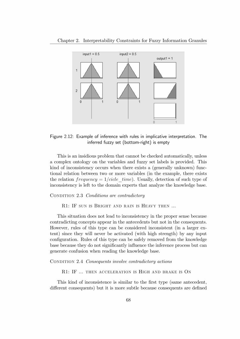
Chapter 2. Interpretability Constraints for Fuzzy Information Granules
Figure 2.12: Example of inference with rules in implicative interpretation. Theinferred fuzzy set (bottom-right) is empty
This is an insidious problem that cannot be checked automatically, unlessa complex ontology on the variables and fuzzy set labels is provided. Thiskind of inconsistency occurs when there exists a (generally unknown) func-tional relation between two or more variables (in the example, there existsthe relation frequency = 1/cicle_time). Usually, detection of such type ofinconsistency is left to the domain experts that analyze the knowledge base.
Condition 2.3 Conditions are contradictory
R1: IF sun is Bright and rain is Heavy then ...
This situation does not lead to inconsistency in the proper sense becausecontradicting concepts appear in the antecedents but not in the consequents.However, rules of this type can be considered inconsistent (in a larger ex-tent) since they will never be activated (with high strength) by any inputconfiguration. Rules of this type can be safely removed from the knowledgebase because they do not significantly influence the inference process but cangenerate confusion when reading the knowledge base.
Condition 2.4 Consequents involve contradictory actions
R1: IF ... then acceleration is High and brake is On
This kind of inconsistence is similar to the first type (same antecedent,different consequents) but it is more subtle because consequents are defined
68
2.6. Constraints on Fuzzy Models
on different Universes of Discourse and inconsistency cannot be checked auto-matically. However, a proper integration of expert knowledge can overcomethe problem by inserting rules that exclude contradictory actions. In theexample the additional rule “if acceleration is greater than zerothen brake is off” enables the automatic detection of an inconsistency.When inconsistency can be automatically detected, it can be assessed by
some quantitative measurements. If the degree of inconsistence degree is toohigh, the knowledge base must be modified so as to improve its consistency.To assess consistency, Jin et al. propose the following measure to be used inthe fitness function of a genetic algorithm (Jin et al., 1998b):
fIncons =RXi=1
RXk=1k 6=i
(1− Cons (Ri, Rk)) (2.89)
where:
Cons (Ri, Rk) = exp
−³S(Ai,Ak)S(Bi,Bk)
− 1´2
(S (Ai,Ak))−2
(2.90)
being S a similarity measure, =Ri = hAi, Bii and =Rk= hAk, Bki. In
(Meesad and Yen, 2002), inconsistency is evaluated as:
RS =2
R (R− 1)RXi=1
RXk=1k 6=i
RS (Ri, Rk) (2.91)
where:
RS (Ri, Rk) =1
n+ 1
nXj=1
¡S¡Aji , A
jk
¢+ eq (Bi, Bk)
¢(2.92)
being Ai = A1i × · · · × Ani , Ak = A1k × · · · × An
k , and eq (Bi, Bk) = 1 ifBi = Bk , 0 otherwise.Consistency of rule-based fuzzy models has also been theoretically ana-
lyzed in the specific context of implicative interpretation. This analysis is wellsynthesized by Pedrycz and Gomide (Pedrycz and Gomide, 1998). Brieflyspeaking, inconsistency is defined at the level of a single fuzzy set and it ismeasured as “The degree to which set is included in the empty set”, i.e.:
c (A) = ν (∅, A) = 1− π (U,A) = 1− supx∈U
µA (x) (2.93)
69
Chapter 2. Interpretability Constraints for Fuzzy Information Granules
being ν the necessity measure that measures the degree of inclusion betweentwo fuzzy sets (Dubois and Prade, 1980).Yager and Larsen use such definition to derive a necessary condition for
two rules to be inconsistent (Yager and Larsen, 1991). Given two rulesR1 andR2 such that =R1 = (A1, B1) and =R2 = (A2, B2), they are α−inconsistent ifthere exist a fuzzy input A such that the fuzzy set B inferred by the modelhas a degree of inconsistency α measured by (2.93). If the two rules areα−inconsistent, then the following inequalities hold:
π (B1, B2) ≤ 1− α (2.94a)
π (A1,A2) ≥ α (2.94b)
The two inequalities formalize the condition of similar antecedents (2.94b)and dissimilar consequents (2.94a).To check whether two rules are potentially inconsistent, the following
function is used:
E (x) = µ¬A1(x)⊗ µ¬A2
(x)⊗ π (B1, B2) (2.95)
If there exists some x for which E (x) < 1 then, potential inconsistency ex-ists and the corresponding α−level can be calculated. Scalpelli and Gomideextended this method to deal with multiple rules by constructing a matrixof fuzzy sets that is subject of computation to derive potential inconsisten-cies among couples of rules (Scarpelli and Gomide, 1994). The authors alsoextend this approach to deal with chaining rules, i.e. rules whose consequentvariables are used as antecedent variables in other rules of the knowledgebase, by using the idea of Agarwal and Taniru (Agarwal and Taniru, 1992).Some observation are noteworthy when analyzing consistency of rule-
based fuzzy models. As previously stated, consistency is a requirement ofclassical expert systems that has been extended to fuzzy models. How-ever, as previously discussed, two interpretations exists of a fuzzy knowledgebase: implicative interpretation and conjunctive interpretation. Implicativeinterpretation is a direct generalization of classical rule-based expert systemwithin the fuzzy framework. In such interpretation, consistency issues occuralso in fuzzy models and can be analyzed in the ways previously illustrated.But the most common interpretation of the fuzzy knowledge base is conjunc-tive, which is not equivalent to the implicative interpretation and gives riseto different considerations.To illustrate the consistency issues in a conjunctive interpretation of fuzzy
rules, a simplified setting can be considered. Let be R a trivial crisp knowl-edge base consisting of only two rules. If such rules are interpreted in a
70
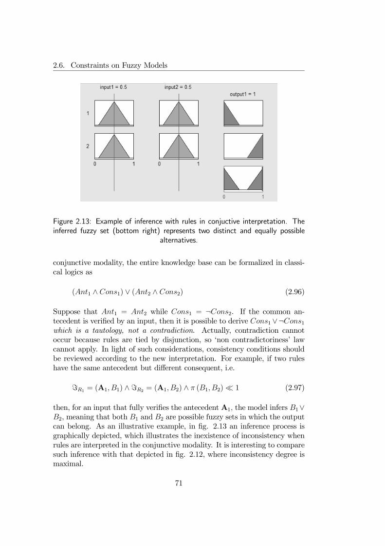
2.6. Constraints on Fuzzy Models
Figure 2.13: Example of inference with rules in conjuctive interpretation. Theinferred fuzzy set (bottom right) represents two distinct and equally possible
alternatives.
conjunctive modality, the entire knowledge base can be formalized in classi-cal logics as
(Ant1 ∧ Cons1) ∨ (Ant2 ∧ Cons2) (2.96)
Suppose that Ant1 = Ant2 while Cons1 = ¬Cons2. If the common an-tecedent is verified by an input, then it is possible to derive Cons1∨¬Cons1which is a tautology, not a contradiction. Actually, contradiction cannotoccur because rules are tied by disjunction, so ‘non contradictoriness’ lawcannot apply. In light of such considerations, consistency conditions shouldbe reviewed according to the new interpretation. For example, if two ruleshave the same antecedent but different consequent, i.e.
=R1 = (A1, B1) ∧=R2 = (A1, B2) ∧ π (B1, B2)¿ 1 (2.97)
then, for an input that fully verifies the antecedent A1, the model infers B1∨B2, meaning that both B1 and B2 are possible fuzzy sets in which the outputcan belong. As an illustrative example, in fig. 2.13 an inference process isgraphically depicted, which illustrates the inexistence of inconsistency whenrules are interpreted in the conjunctive modality. It is interesting to comparesuch inference with that depicted in fig. 2.12, where inconsistency degree ismaximal.
71
Chapter 2. Interpretability Constraints for Fuzzy Information Granules
Model completeness
Constraint 31 (Completeness) For each input, at least one rule musthave non-zero activation strength:
∀x ∈ U∃R ∈ R : =R = (A, B) : µA (x) > 0 (2.98)
Constraint 32 (α-completeness) For a given threshold α, and for eachinput, at least one rule must have activation strength greater than α:
∀x ∈ U∃R ∈ R : =R = (A, B) ∧ µA (x) > α (2.99)
Completeness is a property of deductive systems that has been used in thecontext of Artificial Intelligence to indicate that the knowledge representationscheme can represent every entity within the intended domain. When appliedto fuzzy models, this property informally states that the fuzzy model shouldbe able to infer a proper action for every input (Herrera et al., 1998; Lee,1990). On the other hand, incompleteness is symptom of overfitting (Jinet al., 1999).As stated in (Stamou and Tzafestas, 1999), a complete fuzzy model can
achieve proper operation avoiding undesirable situations. Such undesirablesituations can be easily understood by analyzing the behavior of the fuzzymodel when no rules are activated by an actual input. Suppose that thereexists an input vector that does not activate any rule:
∃x ∈ U∀R ∈ R : =R = (A, B)→ µA (x) = 0 (2.100)
If the “Then” part of the rules is interpreted as conjunction, then thefuzzy sets deriving from the interpretation of each rule are all empty:
∀R ∈ R∀y ∈ UO : = (Rule) [x, y] = 0 (2.101)
As a consequence, the fuzzy set obtained by aggregating rules is the emptyset. The inferred fuzzy set is empty, thus excluding any possible numericaloutcome from the model. Put differently, no action is decided for the giveninput. However, many defuzzification procedures always provide a numericaloutcome even if the inferred fuzzy set is an empty set. This is necessary whenan action is always required from the model (e.g. in control applications).In this case, however, the final outcome is arbitrary and is not a logicalconsequence of the knowledge base embodied in the model.If the “Then” part is interpreted as an implication, a completely opposite
situation is likely to happen. Since material implication is always verified
72
2.6. Constraints on Fuzzy Models
when the antecedent is true, the fuzzy set derived for each rule coincideswith the output Universe of Discourse UO, i.e.:
∀R ∈ R∀y ∈ UO : = (Rule) [x, y] == (Ant)¯ µL−1y (FLy)
(y) = 0¯ µL−1y (FLy)(y) = 1 (2.102)
The conjunctive aggregation of all rules coincides to the output Universe ofDiscourse, hence the inferred fuzzy set gives full possibility to any element ofthe Universe of Discourse and the defuzzification procedure can legitimatelychoose any random element from this Universe. As a consequence, the be-havior of the fuzzy model is undefined in input regions where no rules arefired. Undesirable situations may occur even if some rule is fired by the input,but the activation strength is too low. This phenomenon is also called “weakfiring”. For such reason, stronger α-completeness is preferred over simplecompleteness to guarantee a proper behavior of the fuzzy model (Pedrycz,1993).Between the two forms of completeness, namely completeness of the
Frames of Cognition (coverage) and completeness of the model, the formeris more often required in interpretable fuzzy modeling even though modelincompleteness can lead to undesirable situations as those previously illus-trated. Clearly model completeness implies completeness of Frames of Cog-nition, but the contrary is not true unless the knowledge base is composedof rules defined by all possible combinations of antecedent fuzzy sets. How-ever, all combinations of fuzzy sets lead to a combinatorial explosion of thenumber of rules, making the model impractical.In addition, often the input space has nonuniform possibility distribu-
tion but the multidimensional Universe of Discourse is defined as Cartesianproduct of one-dimensional fuzzy sets for interpretability pursuits. As a con-sequence, the multidimensional Universe of Discourse may be only a supersetof the plausible domain in which input data effectively belong, while inputsnot belonging to such domain can be considered as outliers. In such situa-tion, model incompleteness can be tolerated since undesirable behavior mayresult only in regions of the Universe of Discourse where inputs are unlikelyto occur.If outliers have to be properly handled by a fuzzy model, model complete-
ness should be restored but, in order to avoid combinatorial rule explosion,two approaches may be used:
• Infinite support fuzzy sets can be adopted in the design of the Framesof Cognition. In such case, all inputs of the Universe of Discourse acti-vate all rules. This approach is simple but may decrease the inferenceefficiency and can originate the weak-firing phenomenon;
73
Chapter 2. Interpretability Constraints for Fuzzy Information Granules
• A “default rule” can be introduced (Peña-Reyes and Sipper, 2003;Vuorimaa, 1994). A default rule is a special rule that is activated onlywhen no rules of the remaining knowledge base are fired. The defaultrule may be associated with a special output signaling ‘out of rangeoperation’ or an indecision status. Default rules may be crisp or fuzzy.In the latter case, the activation strength is defined as the complementof the maximum activation strength among all ordinary rules. Defaultfuzzy rules can be thus used to fight the weak-firing phenomenon butits semantics must be carefully defined due to its special role in thefuzzy model.
Number of variables
Constraint 33 The number of input and output variables should be assmall as possible
The number of input/output variables are strictly related to the dimen-sionality of the input/output Universes of Discourse. A high number of in-put/output variables is negative in fuzzy modelling for several reasons, suchas:
1. The length of each rule becomes to high, thus hampering interpretabil-ity. Unless sophisticated techniques are adopted to reduce the numberof variables in each rule (see 2.5), a high number of variables — typicallymore than seven — reduces the readability of the knowledge base;
2. Fuzzy models are usually acquired from data by means of identificationtechniques. Like all data-identified models, fuzzy models are subject ofthe so-called “curse of dimensionality” (Bellman, 1961). According toBellman, the number of parameters needed for approximating a func-tion to a prescribed degree of accuracy increases exponentially with thedimensionality of the input space (Haykin, 1999)25. In fuzzy models,such parameters correspond to the number of fuzzy sets and the num-ber of fuzzy rules. The basic reason for the curse of dimensionality isthat a function defined in high dimensional space is likely to be muchmore complex than a function defined in a lower dimensional space,and those complications are harder to discern (Friedman, 1995).
25The complete formulation of the curse of dimensionality also involves a “smoothingfactor” that measures the oscillatory nature of the approximating function and is assumedconstant as the number of dimensions increases. For the sake of simplicity — motivatedby the qualitative level of the discussion — such smoothing factor has not been consideredhere.
74

2.6. Constraints on Fuzzy Models
According to the above-mentioned motivations, the number of input vari-ables and that of output variables have a different effect on the model degra-dation. Specifically, while a high number of output variables hampers theinterpretability of the model by lengthening the rules, a high number of inputvariables damages interpretability and causes the curse of dimensionality. Forsuch reason, input and output variables are treated differently in the attemptof reducing their number.
Input variables The reduction of the number of input variables can im-prove the readability of the knowledge base and avoids the curse of dimen-sionality. Clearly, a drastic reduction of the number of input variables reducesthe number of free parameters in the model and, consequently, the ability ofidentifying a large set of functions. For such reason, any technique to reducethe number of input variables must be balanced with the desired accuracyof the final model. In literature, there exists an impressive number of tech-niques to reduce the number of input variables, which can be classified intwo main categories:
Feature extraction Themultidimensional Universe of DiscourseU is trans-formed into another multidimensional Universe of Discourse U0 with adimensionality lower than U. Such transformation is usually achievedby exploiting the distribution of an available dataset and can be linearon non-linear. There is a wide number of feature extraction techniquesand a review of them can be found in (Jain et al., 2000). While effec-tive for black-box models, feature extraction techniques are dangerousin interpretable fuzzy models because the new set of variables comingfrom the transformed Universe of Discourse U0 cannot be associated toany physical meaning. For such reason, feature extraction techniquesshould be avoided in interpretable fuzzy modelling.
Feature selection Feature selection techniques aim to extract a small sub-set of input variables without degrading too much the accuracy of thefuzzy models. Differently to feature extraction techniques, feature se-lection does not destroy interpretability because the selected input vari-ables are not new but a subset of the original variables. As a conse-quence, the physical meaning associated to each variable is retained.Feature selection is less effective than feature extraction, but it is nec-essary when interpretability is the major concern of a fuzzy model. Awide number of feature selection techniques exists in literature, butthose that are especially suited for interpretable fuzzy modelling definea ranking of features before selecting a subset of them. In feature rank-ing, an ordered list of input variables is provided, where the higher is
75

Chapter 2. Interpretability Constraints for Fuzzy Information Granules
the position of the variable the higher is its influence in determining theinput/output relation captured by the fuzzy model (Linkens and Chen,1999). Such ordered list is very useful for interpretable fuzzy modelingbecause it offers an interaction tool with the domain experts, who candecide to force some input variables into the model — perhaps becausetheir physical meaning is essential — or to discard some input variableseven though their relative position in the list is high. Such decisionare better supported if the ordered list is associated with a correlationanalysis, which can ensure that the elimination of some variables doesnot hamper the overall accuracy of the model, when highly correlatedvariables still remain in the ranked list.
Output variables Throughout this Chapter the number of variables of themodel has been assumed to be only one, but in many applicative problemsthe number of variables can be very high. Two approaches can be used todeal with a high number of output variables: building a single Multi-InputMulti-Output (MIMO) model or defining several Multi-Input Single-Output(MISO) models.
MIMO Models A MIMO fuzzy model is defined by rules where the con-sequent is a conjunction of two or more fuzzy constraints. Usually,the inference procedure of a MIMO model operates by inferring theoutput value of each variable independently. This is possible becauseof the conjunctive relation of the output fuzzy constraints26. Whenthe number of output variables is too high, rules of MIMO models be-come illegible and must be replaced by models with simpler knowledgerepresentation;
MISO Models A MISO model is defined by rules with a single consequent.When multiple outputs are required, several MISO models are defined,one for each output variables. The main advantage of MISO mod-els is legibility of the rule base, which is simpler than MIMO models.Moreover, since MISO models are identified independently, the result-ing knowledge bases are better suited to represent the input/outputrelationships for each output variable. A consequent benefit is thegreater accuracy of MISO models w.r.t. a single MIMO model (thisaccuracy improvement is also justified by the increased number of free
26Some authors generalize the definition of rules by including also disjunctive conse-quents (Pedrycz and Gomide, 1998). In such case, however, inference cannot be accom-plished independently for each output variable. For such reason, disjunctive consequentsare very rare in fuzzy modeling.
76
2.6. Constraints on Fuzzy Models
parameters that characterize a family of MISO models with respect toa single MIMO model). The main drawback of MISO models is thatthe Frames of Cognition of the same input variable are identified in-dependently for each model. As a result, Frames of Cognition for thesame linguistic variable may have the same linguistic labels but dif-ferent semantics. This situation of ambiguity clearly impedes a clearunderstanding of the acquired knowledge, hence MISO models shouldbe avoided if interpretability is of major concern.
Granulated output
Constraint 34 The output of the fuzzy model should be an informationgranule rather than a single numerical value
In most cases, fuzzy models are used to identify an unknown input/outputmapping defined on numerical domains. Even though information is processedwithin the model by means of fuzzy sets manipulation, often the required out-come is a single numerical value that must be used in the environment fordecision making, classification, control, etc. In other cases, the outcome ofthe fuzzy model is just an information for further processing (e.g. in med-ical diagnosis, the outcome of the fuzzy model can be used by physicians toactuate a proper decision). In situations like this latter, it is favorable thatthe output of the fuzzy model would be an information granule rather thana single numerical value. Indeed, granular information is richer than numer-ical information because the former also conveys uncertainty or vaguenessinformation that are valuable in a decision making process.
A first approach to provide granulated information is to avoid the de-fuzzification procedure and just return the resulting fuzzy set attained byaggregating the outcomes inferred by each rule. Such fuzzy set providesvagueness information about the model output but can be hard to interpretbecause it generally does not satisfy none of the interpretability constraintsfor fuzzy sets. An alternative approach consists in enriching the numericaloutcome provided by the defuzzificator with uncertainty information aboutthe behavior simulated by the fuzzy model. This new information can bewell represented by means of prediction intervals. A successive Chapter isdevoted at describing a proposed method for integrating prediction intervalswithin fuzzy models.
77
Chapter 2. Interpretability Constraints for Fuzzy Information Granules
2.7 Constraints on Fuzzy Model Adaption
Fuzzy information granules are often used as building blocks for designingrule-based fuzzy models, which can be effectively used to solve soft-computingproblems such as predictions, classifications, system identification, etc. Froma functional point of view, fuzzy models are approximative representations ofan underlying functional input/output relationship that has to be discovered.To achieve such objective, often a dataset is available, which provides a finitecollection of input/output examples from which the model’s knowledge hasto be built. Information granulation techniques operate on such dataset toproperly extract information granules that will be used to define the knowl-edge base. In such context, information granulation can be accomplished intwo main ways:
1. The complete dataset of examples is granulated, involving both inputand output information. At the end of the granulation process, theknowledge base of the fuzzy model is complete and can be immediatelyused for approximating the underlying functional relationship. A typ-ical example of fuzzy model defined by this kind of knowledge base isthe Mamdani Fuzzy Inference System;
2. The examples are split in the input and output components, and thegranulation process is executed only in the input part. This choice istypical in classification problems, where outputs are class labels thatbelong to a symbolic domain that cannot be granulated. This formof granulation is also chosen when accuracy has a great impact in theassessment of the model quality.
When the second form of granulation is chosen, the resulting informationgranules are able to describe the relationships among input data, but theymiss to correctly represent the underlying input/output relationship. There-fore the knowledge base of the fuzzy model has to be refined (or adapted) inorder to better approximate the unknown functional relationship by meansof supervised learning schemes27.In an extreme synthesis, the adaption of a fuzzy model can be viewed as
a transformation
L (M,D) =M0 (2.103)
27It should be noted that information granulation on the input space can be consideredas an unsupervised learning scheme. The fuzzy model resulting from both unsupervisedand supervised learning is then a hybrid model.
78

2.7. Constraints on Fuzzy Model Adaption
that maps an original model M into a new modelM0 with the support ofa finite set of examples D. The transformation is aimed at optimizing anobjective function ℘ such that:
℘ (M0) ≥ ℘ (M) (2.104)
The objective function may be a measure of accuracy, generalization abil-ity, interpretability, etc. or a combination of these28. Even though it is notthe general case, it is assumed hereafter that the adaption process does notmodify the structure of the Frames of Cognition involved in the model, i.e.their number, their cardinality and labelling. What is usually changed by thelearning process are the free parameters that characterize input and outputfuzzy sets. In some cases, the information granules of the rules are changedby removing useless soft-constraints. The rule structure is admitted to chang-ing, e.g. by removing useless rules or adding new ones. With a slight abuse ofnotation, hereafter each element X belonging to the model (especially fuzzysets) that are subject to adaptation by means of L will be indicated withLX.There exist several methods to adapt a model to data, but most of them
fall in two main paradigms:
Genetic Algorithms The fuzzy model is adapted by evolving its structureand/or its free parameters. Three classical approaches may be adoptedto adapt fuzzy models to data:
Michigan Approach (Michalewicz, 1996) Each individual representsa single rule. The knowledge base is represented by the entire pop-ulation. Since several rules participate in the inference process,the rules are in constant competition for the best action to beproposed, and cooperate to form an efficient fuzzy model. Such co-operative/competitive necessitates an effective credit-assignmentpolicy to ascribe fitness values to individual rules.
Pittsburgh Approach (Michalewicz, 1996) Each individual is a can-didate knowledge base. Genetic operations provide new popula-tions of knowledge bases that can be evaluated for their accuracybut also for additional properties such as transparency. The maindrawback of this approach is the computational cost.
Iterative Rule Learning Approach (Herrera et al., 1995) This ap-proach is used to both identify and refine fuzzy models by first
28A complete and self-contained functional model for supervised learning can be foundin (Vapnik, 1999).
79

Chapter 2. Interpretability Constraints for Fuzzy Information Granules
providing a model with a single rule, then new rules are addeduntil an appropriate knowledge base is defined.
In recent years, a new promising approach for genetic optimization has beenproposed, which appears particularly suitable to find fuzzy models bal-anced in accuracy and interpretability. These “multi-objective” ge-netic algorithms allow for searching multiple solutions in parallel withthe aim of optimizing several fitness functions simultaneously (Fon-seca and Fleming, 1995). Multi-objective genetic algorithms have beensuccessfully used to design and refine fuzzy models from data by si-multaneously optimizing conflicting fitness functions such as accuracyand interpretability (Jiménez et al., 2001; Gómez-Skarmeta et al., 1998;Ishibuchi et al., 1997).
Neuro-Fuzzy Networks The fuzzy model is converted into a specific neu-ral network, which is trained according to some neural learning scheme.After learning, the neural network is re-converted back into a fuzzymodel. Two approaches for neuro-fuzzy modeling are very common(Nauck and Kruse, 1994):
Cooperative approach The neural network and the fuzzy model aredistinct objects that cooperate to form an accurate final model.For example, the neural network can be used to define a propershape of fuzzy sets, or a proper weight of rules, while the fuzzymodel is responsible in making the input/output mapping;
Hybrid approach There exist a bijective mapping from nodes of theneural network and the components of the fuzzy model, so thatthe two models can be viewed as two facets of the same system,called “neuro-fuzzy network”. This kind of architecture is called“translational” in the Knowledge-Based Neurocomputing para-digm (Cloete and Zurada, 2000), because the fuzzy model can beconverted into the neural network and vice-versa in every stageof processing. One of the first neuro-fuzzy networks appeared inliterature is ANFIS (Adaptive Network-based Fuzzy Inference Sys-tem) (Jang, 1993). Actually, the hybrid approach has overcomethe cooperative approach because of its versatility and efficacy.
In interpretable fuzzy modelling, the adaption process must not destroythe interpretability constraints, i.e. the adapted model M0 must satisfy atleast the same interpretability constraints of the original model M. Moreconstraints can be added if the objective of adaption is interpretability im-provement. If — as often occurs — the adaption process is iterative, the
80
2.7. Constraints on Fuzzy Model Adaption
intermediate models emerging after each iteration may not satisfy the in-terpretability constraints. This is usually the case when adaption is carriedout by means of regularized learning (Bishop, 1995) or when interpretabilityconstraints are applied after several adaption stages for efficiency pursuits(Altug et al., 1999). However, when the adaption process can be haltedat every stage (e.g. to allow user interaction or in real-time applicative con-texts) it is more desirable that all intermediate models satisfy interpretabilityconstraints (Nauck et al., 1997).In addition to the previously discussed interpretability constraints, the
adaption process must be designed so as to not twisting the semantics of thefuzzy sets involved in the knowledge base. Indeed, the adaption of the modelhas the role of refine and not completely modify the meaning conveyed by theknowledge base. For such reason, additional constraints could be requiredon the adaption process for interpretable fuzzy modelling.
No position exchange
Constraint 35 Two fuzzy sets belonging to the same Frame of Cognitionmust not exchange position after learning:
∀F ∈ FI ∪ FO ∀A,B ∈ F : A ≺ B → LA ≺ LB (2.105)
This criterion, elicited by Nauck and Kruse, assures that the learningprocess does not switch the meaning of two linguistic labels associated tofuzzy sets belonging to a Frame of Cognition (Nauck and Kruse, 1998). Thisis especially important when linguistic labels express qualities on the Universeof Discourse, like Low, Medium and High. It would be indeed undesirablethat, after learning, fuzzy sets associated to these labels exchange their po-sition such that the final order does not reflect the metaphors of the labels,e.g. when Low ≺ High ≺ Medium. Note that a relabelling operation ispossible so as to restore the semiotic ordering of linguistic labels, but this op-eration is against the aims of model adaptation, according to which the modelshould be only finely tuned to better meet the objective function. In such aviewpoint, any relabelling operation would be seen as a model re-design.When labels express vague quantities (like about_2) ore precise quan-
tities (as in the consequents of Takagi-Sugeno rules), position exchange isadmissible provided that the label changes in agreement to the fuzzy sets.In such case, re-labelling is an admissible operation because the fuzzy setsexpress quantities that are susceptible to changes during the tuning process.
81

Chapter 2. Interpretability Constraints for Fuzzy Information Granules
No sign change
Constraint 36 Fuzzy sets with cores in positive (resp. negative) rangemust not change sign after learning:
∀F ∈ FI ∪ FO ∀A ∈ F : min coreA ≥ 0→ min coreLA ≥ 0 (2.106)
∀F ∈ FI ∪ FO ∀A ∈ F : max coreA ≤ 0→ max coreLA ≤ 0 (2.107)This criterion is mostly related to fuzzy sets used to express vague quan-
tities (Nauck et al., 1997; Nauck and Kruse, 1998). Informally speaking, thecriterion states that if a fuzzy set represents a signed quantity (either positiveor negative), then the corresponding fuzzy set resulting from adaption mustrepresent a quantity with the same sign. In this way, the learning processL does not drastically change the semantics of the knowledge base duringfine-tuning. Note that if a fuzzy set is unimodal and satisfies the “NaturalZero Positioning” constraint, i.e. coreA = 0, then the “No Sign Change”constraint requires that, after adaption, the refined fuzzy set still representsthe number 0, since coreLA= 0. As Natural Zero Positioning can be ex-tended to “Natural S Positioning” (see 2.3), also the following constraintscan be formulated:
∀s ∈ S ∀F ∈ FI ∪ FO ∀A ∈ F :min coreA ≥ s → min coreLA ≥ s (2.108)
and
∀s ∈ S ∀F ∈ FI ∪ FO ∀A ∈ F :max coreA ≤ s → max coreLA ≤ s (2.109)
Similarity preservation
Constraint 37 Any adapted fuzzy set should be similar to the original one:
∀F ∈ FI ∪ FO ∀A ∈ F : S (A,LA) ≈ 1 (2.110)
where S is a similarity measure.
This constraint informally states that fuzzy sets subject of adaption mustnot change too much in order to preserve their original semantics. Theformalization of the criterion is a generalization of the work of Lotfi, who usesa rough-fuzzy representation of Gaussian membership functions to restrictthe variability of parameters (namely, center and width) into a predefinedrange (Lotfi et al., 1996). This constraint captures the very nature of fine
82
2.8. Final remarks
tuning, i.e. adaption of the model without excessive modification of theinternal knowledge. On the other hand, it should be observed that if theadaption process leads to a strong modification of the model, than a badinitial design of the model could be hypothesized. In such a case, a completeredesign of the model should be considered.
2.8 Final remarks
Thoroughly this Chapter, a number of interpretability constraints have beensurveyed. Some of these constraints are mandatory for interpretable fuzzy in-formation granulation, while others can be included or dropped from a designstrategy according to subjective judgements. Furthermore, the applicationof some interpretability constraints depends on the final representation of theinformation granules, and, in general, of the knowledge base. As an example,some interpretability constraints make sense only for information granulesrepresenting qualities on the Universe of Discourse, while other constraintsare especially suited for information granules representing fuzzy quantities.Additional interpretability constraints can be added for specific applica-
tive needs. As an example, in (Johansen et al., 2000) a number of special-purpose interpretability constraints have been proposed for system identifica-tion applications. Because of limited interest, special-purpose interpretabilityconstraints have not been considered in this Chapter, rather preferring gen-eral purpose constraints because of their wider applicability. In summary, onthe engineering standpoint, a number of issues should be taken into accountin the selection of interpretability constraints, including:
• Type of representation of information granules (e.g. qualitative vs.quantitative information granules);
• Type of fuzzy model (e.g. Mamdani vs. Takagi-Sugeno models);• Concerns of modelling: accuracy, efficiency, interpretability;• Epistemological assumptions (e.g. implicative vs. conjunctive rules);• Applicative context.
Scientific investigation on interpretability constraints is still open. Fur-ther inquiries in the field may include the analysis of interpretability ondifferent types (e.g. discrete) of Universes of Discourse. Also, the integra-tion of feature extraction techniques within interpretable fuzzy information
83

Chapter 2. Interpretability Constraints for Fuzzy Information Granules
granulation is of great interest (e.g. to form complex linguistic constraintssuch as “Product of Volume and Pressure is Low”).Within Cognitive Science, interpretability constraints may provide a valid
help in understanding the mechanisms of human behavioral phenomena likeconceptual model building and explanation. In this context, the integrationof results coming from different disciplines could be highly benefic. As an em-blematic example, the psychological experiments of Miller in (Miller, 1956)provide a better understanding of human abilities as well as important guide-lines for interpretable fuzzy information granulation and modelling. The ex-ample sheds light on the inter-disciplinary character of interpretable fuzzyinformation granulation, which results a promising theoretical framework forbringing machines nearer to humans with the aid of perception-based com-puting.
84
Part II
Theoretical Contributions toInterpretabilty in FuzzyInformation Granulation
85

Chapter 3
DistinguishabilityQuantification
3.1 Introduction
Distinguishability of fuzzy sets is one of the most common interpretabilityconstraints adopted in literature. In brief, distinguishability can be viewedas a relation between fuzzy sets defined on the same Universe of Discourse.Distinguishable fuzzy sets are well disjunct so as to represent distinct con-cepts and can be associated to metaphorically different linguistic labels. Welldistinguishable fuzzy sets provide the following advantages within the Theoryof Fuzzy Information Granulation:
• Obviate the subjective establishment of membership-function/linguisticterm association (Valente de Oliveira, 1998);
• Avoids potential inconsistencies in fuzzy models (Valente de Oliveira,1999b);
• Reduce model’s redundancy and consequently computational complex-ity (Setnes et al., 1998a);
• Linguistic interpretation of the fuzzy information granules is easier(Setnes et al., 1998a);
Completely disjunct fuzzy sets are maximally distinguishable. However,disjunct fuzzy sets may violate some other interpretability constraints (e.g.coverage), hence partially overlapping fuzzy sets are more preferable for thedefinition of interpretable fuzzy information granules.
87

Chapter 3. Distinguishability Quantification
Distinguishability quantification can be realized in different ways. Themost adopted characterization is by means of similarity measures. In (Setneset al., 1998a) similarity measures are deeply discussed in the context of fuzzymodelling. There, similarity is interpreted as a fuzzy relation defined overfuzzy sets and corresponds to the “degree to which two fuzzy sets are equal”.Such interpretation is then formally characterized by a set of axioms.Similarity measures well capture all the requirements for distinguishable
fuzzy sets, but their calculation is usually computationally intensive. Asa consequence, most strategies of model building that adopt similarity mea-sures for interpretability enhancement are based on massive search algorithmssuch as Genetic Algorithms (Roubos and Setnes, 2001; Meesad and Yen,2002; Setnes et al., 1998b), Evolution Strategies (Jin, 2000), Symbiotic Evo-lution (Jamei et al., 2001), Coevolution (Peña-Reyes and Sipper, 2003), orMulti-Objective Genetic Optimization (Jiménez et al., 2001). Alternatively,distinguishability improvement is realized in a separate design stage, oftenafter some data driven procedure like clustering, in which similar fuzzy setsare usually merged together (Paiva and Dourado, 2001; Setnes et al., 1998a).When the distinguishability constraint has to be included in less time con-
suming learning paradigms, like neural learning, similarity measure is seldomused. In (Paiva and Dourado, 2001), after a merging stage that uses simi-larity, fine tuning is achieved by simply imposing some heuristic constraintson centers and width of membership functions. In (Jin and Sendhoff, 2003),a distance function between fuzzy sets (restricted to the Gaussian shape) isused in the regularization part of the RBF1 cost function. In (Guillaume andCharnomordic, 2004) a sophisticated distance function is used to merge fuzzysets. In (Nauck and Kruse, 1998; Espinosa and Vandewalle, 2000; Castellanoet al., 2002) the possibility measure is adopted to evaluate distinguishability.The possibility measure has been intensively studied within Fuzzy Set
Theory and has some attracting features that promote a deeper investiga-tion in the context of distinguishability assessment. Although it is not asimilarity measure, it has a clear and well-established semantics since it canbe interpreted as the degree to which a flexible constraint “X isA” is sat-isfied (Zadeh, 1978; Toth, 1999). In addition, the possibility quantificationof two fuzzy sets can be often analytically expressed in terms of fuzzy sets’parameters. This makes possibility evaluation very efficient so that it can beeffortlessly embodied in computationally inexpensive learning schemes.The objective pursued in the Chapter is to derive some significant re-
lationships between similarity and possibility measures. Specifically, somesufficient conditions are demonstrated to positively correlate possibility and
1Radial Basis Function neural network
88
3.2. Distinguishability measures
similarity in the worst case, i.e. the lower is the possibility between twofuzzy sets, the lower is the upper-bound of similarity that can be measuredbetween the same fuzzy sets. As a final result, some theorems formally provethat, under some mild conditions, any transformation aimed to reduce possi-bility between fuzzy sets actually reduces also their similarity measure and,consequently, improves their distinguishability. In light of such theoretical re-sults, the possibility measure emerges as a good candidate for interpretabilityanalysis as well as for efficient interpretable fuzzy modelling.
3.2 Distinguishability measures
In this Section the most common measures to quantify distinguishabilityare formalized and briefly described. A deep description is provided forthe similarity and the possibility measures, since they are subject of furtherinvestigation in successive sections. Other measures proposed in literatureare also surveyed, and some theoretical results for them are established.For the sake of clarity, the adopted formal notation is repeated here. In
this context any fuzzy set is denoted with a capital letter (A, B, etc.) andthe corresponding membership function with µA, µB, etc. Each membershipfunction is defined on the same Universe of Discourse U, which is assumed tobe a one-dimensional closed interval [mU ,MU ] ⊂ R. The set of all possiblefuzzy (sub-)sets defined over U is denoted with F (U), while the finite familyof fuzzy sets actually involved in a fuzzy model is called “Frame of cognition”and it is denoted with F.
3.2.1 Similarity measure
According to (Setnes et al., 1998a), the similarity measure between two fuzzysets A and B is a fuzzy relation that expresses the degree to which A and Bare equal. Put formally, similarity is a function:
S : F (U)×F (U)→ [0, 1] (3.1)
such that:
1. Non-overlapping fuzzy sets are totally non-similar and vice versa2:
S (A,B) = 0 ⇐⇒ ∀x ∈ U : µA (x)µB (x) = 0 (3.2)
2In (Setnes et al., 1998a) another definitory property states that overlapping fuzzy setsmust have similarity greater than zero. However, this is a direct consequence of property1 and definition of S.
89

Chapter 3. Distinguishability Quantification
The latter definition, given in (Setnes et al., 1998a), may not be satis-factory for fuzzy sets that overlap in a finite (or countable) number ofpoints. In such case, similarity can be still zero even if the fuzzy setsdo overlap (see, e.g. example 3.1). In a more precise formalization theleft-to-right implication would be truncated.
2. Only equal fuzzy sets have maximum similarity:
S (A,B) = 1 ⇐⇒ ∀x ∈ U : µA (x) = µB (x) (3.3)
The same objection for property 1 could be stated for fuzzy sets thatare equal everywhere except in a finite (or countable) number of points.Even in this case, the left-to-right implication would be truncated.
3. The similarity measure is invariant under linear scaling of the fuzzysets, provided that the scaling is the same:
S (A,B) = S (A0, B0) (3.4)
where:
∃k 6= 0∃l ∈ R : µA (x) = µA0 (kx+ l)µB (x) = µB0 (kx+ l)
(3.5)
Property 1 assures that mutually exclusive fuzzy sets are not similar at all,while property 2 assures that equal fuzzy sets are totally similar. Property 3establishes that similarity between fuzzy sets does not change if the Universeof Discourse changes according to a linear transformation of its values (e.g.if two temperatures are similar when expressed Celsius degrees, they mustremain similar also when expressed in Fahrenheit degrees).For sake of completeness, the following symmetry property is added,
which makes similarity more adherent to the informal definition of “degreeof equality”:
4. Similarity is a symmetrical function:
S (A,B) = S (B,A) (3.6)
Several similarity measures have been proposed in literature, and someof them can be found in (Cross, 1993; Setnes, 1995). However, in inter-pretability analysis, the most commonly adopted similarity measure is thefollowing:
90
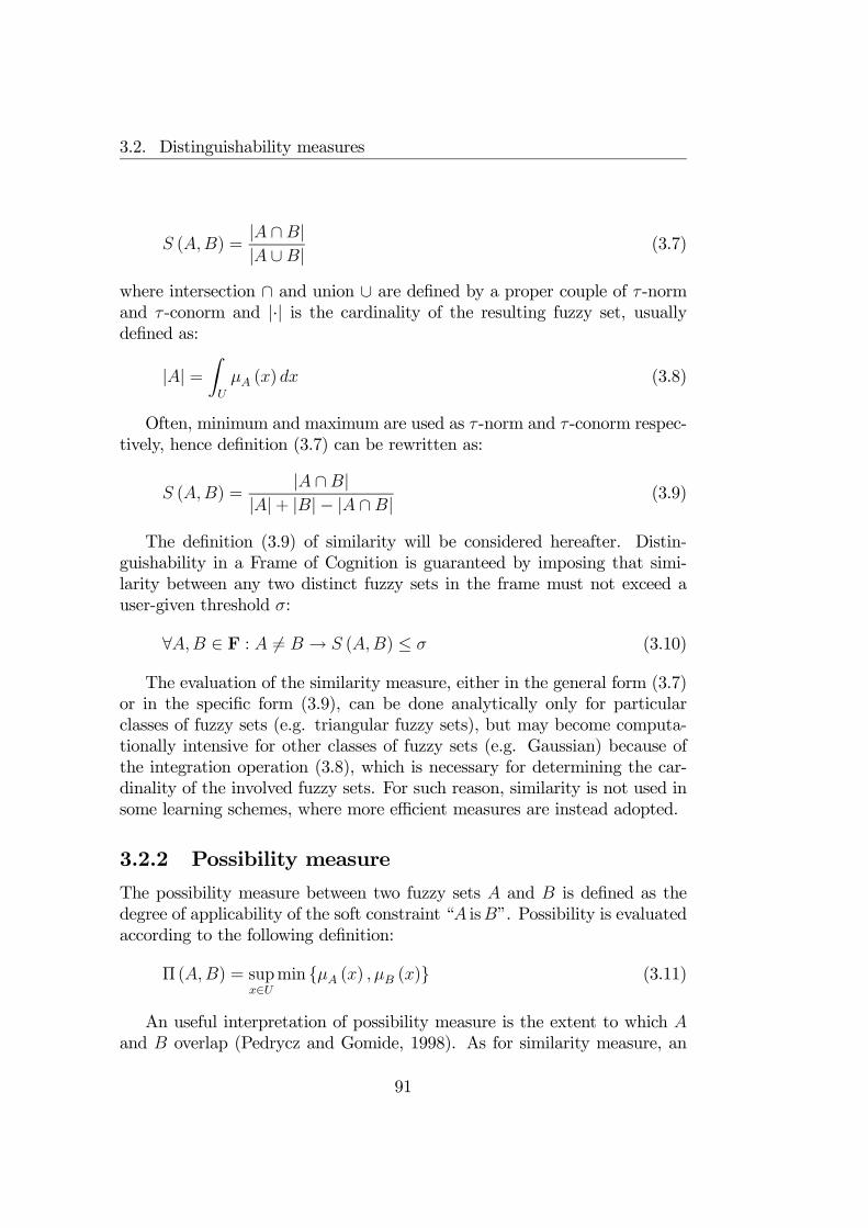
3.2. Distinguishability measures
S (A,B) =|A ∩B||A ∪B| (3.7)
where intersection ∩ and union ∪ are defined by a proper couple of τ -normand τ -conorm and |·| is the cardinality of the resulting fuzzy set, usuallydefined as:
|A| =ZU
µA (x) dx (3.8)
Often, minimum and maximum are used as τ -norm and τ -conorm respec-tively, hence definition (3.7) can be rewritten as:
S (A,B) =|A ∩B|
|A|+ |B|− |A ∩B| (3.9)
The definition (3.9) of similarity will be considered hereafter. Distin-guishability in a Frame of Cognition is guaranteed by imposing that simi-larity between any two distinct fuzzy sets in the frame must not exceed auser-given threshold σ:
∀A,B ∈ F : A 6= B → S (A,B) ≤ σ (3.10)
The evaluation of the similarity measure, either in the general form (3.7)or in the specific form (3.9), can be done analytically only for particularclasses of fuzzy sets (e.g. triangular fuzzy sets), but may become computa-tionally intensive for other classes of fuzzy sets (e.g. Gaussian) because ofthe integration operation (3.8), which is necessary for determining the car-dinality of the involved fuzzy sets. For such reason, similarity is not used insome learning schemes, where more efficient measures are instead adopted.
3.2.2 Possibility measure
The possibility measure between two fuzzy sets A and B is defined as thedegree of applicability of the soft constraint “A isB”. Possibility is evaluatedaccording to the following definition:
Π (A,B) = supx∈U
min µA (x) , µB (x) (3.11)
An useful interpretation of possibility measure is the extent to which Aand B overlap (Pedrycz and Gomide, 1998). As for similarity measure, an
91

Chapter 3. Distinguishability Quantification
−1 −0.5 0 0.5 1 1.5 2 2.5 30
0.5
1
U
Mem
bers
hip
degr
ee
Figure 3.1: Example of fuzzy sets with full possibility but zero similarity
overlapping threshold ϑ can be imposed between any two fuzzy sets in aFrame of Cognition:
∀A,B ∈ F : A 6= B → Π (A,B) ≤ ϑ (3.12)
Some important considerations are noteworthy for possibility measure,especially in comparison with the definition of similarity measure. First ofall, the possibility measure is not a similarity measure because properties 2and 3 for similarity measures are not verified. Moreover, in general there isnot any monotonic correlation between possibility and similarity as showedin the following two examples.
Example 3.1 Let A and B be two crisp sets defined as closed intervals [0, 1]and [1, 2] respectively (see fig. 3.1). Suppose that intersection and unionoperations are defined by the minimum and maximum operators respectively.Then:
S (A,B) =|A ∩B||A ∪B| =
|1||[0, 2]| =
0
2= 0 (3.13)
On the other hand, the possibility measure has a very different value:
Π (A,B) = supx∈[0,2]
min µA (x) , µB (x) = supx∈[0,2]
½0, x 6= 11, x = 1
= 1 (3.14)
This result is coherent with the definition of the two measures. Indeed, the twointervals are quasi-disjunct (i.e. disjunct everywhere except in a single point),hence their similarity should be very low (zero using the standard definition(3.9)). On the other hand there is the full possibility that an element of theUniverse of Discourse belongs both to A and B, hence the possibility measureis maximal.
92

3.2. Distinguishability measures
−1 0 1 2 30
0.2
0.4
0.6
0.8
1
U
Mem
bers
hip
degr
ee
Figure 3.2: Example of fuzzy set with low possibility
Example 3.2 Let A be a fuzzy set defined over the entire Universe of Dis-course U with constant membership function 0 < ε¿ 1 (see fig. 3.2). Then,by definition:
S (A,A) = 1 (3.15)
but:
Π (A,A) = supx∈U
µA (x) = ε (3.16)
Here, again, the similarity is maximal as a correct formalization of “degreeof equality”. On the other hand, the possibility is very low since it is veryunlikely (or undesirable, etc.) that an element belongs to the fuzzy set A.
The previous examples show that the possibility measure cannot be usedto evaluate similarity between two fuzzy sets. Nevertheless, the possibilitymeasure has features that are important in distinguishability analysis:
1. The possibility threshold ϑ has a clear semantics as it can be interpretedin the context of Possibility Theory (Dubois and Prade, 1988). On theother hand, the similarity threshold σ has a more arbitrary nature(it also depends on the specific definition of intersection and unionoperators);
2. Numerical integration is not necessary when calculating possibility, incontraposition with similarity calculation. Moreover, although the gen-eral definition (3.11) may require a numerical sampling of the Universeof Discourse, the possibility measure can be evaluated analytically forseveral classes of membership functions (e.g. triangular, Gaussian, bell-shaped, etc., see table 3.1 for an example). This feature enables theadoption of possibility measure in efficient learning schemes;
93
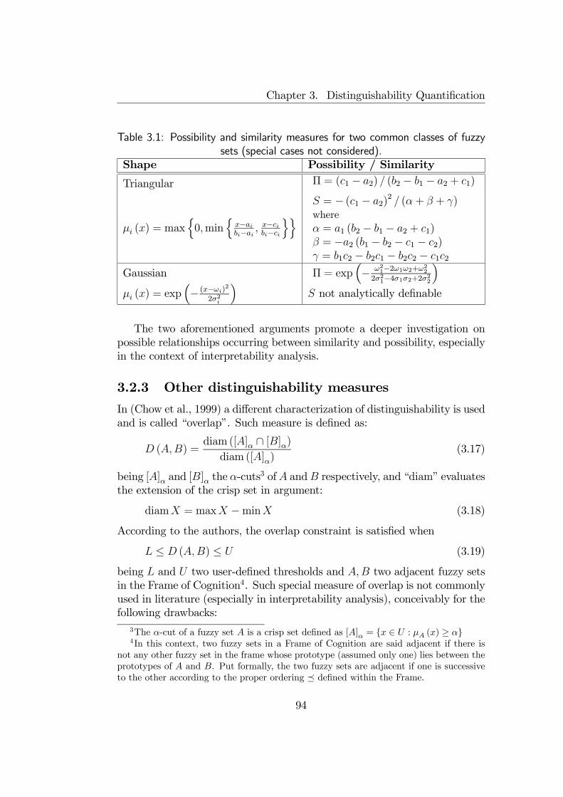
Chapter 3. Distinguishability Quantification
Table 3.1: Possibility and similarity measures for two common classes of fuzzysets (special cases not considered).
Shape Possibility / Similarity
Triangular Π = (c1 − a2) / (b2 − b1 − a2 + c1)
µi (x) = maxn0,min
nx−aibi−ai ,
x−cibi−ci
oo S = − (c1 − a2)2 / (α+ β + γ)
whereα = a1 (b2 − b1 − a2 + c1)β = −a2 (b1 − b2 − c1 − c2)γ = b1c2 − b2c1 − b2c2 − c1c2
Gaussian Π = exp³− ω21−2ω1ω2+ω222σ21−4σ1σ2+2σ22
´µi (x) = exp
³− (x−ωi)2
2σ2i
´S not analytically definable
The two aforementioned arguments promote a deeper investigation onpossible relationships occurring between similarity and possibility, especiallyin the context of interpretability analysis.
3.2.3 Other distinguishability measures
In (Chow et al., 1999) a different characterization of distinguishability is usedand is called “overlap”. Such measure is defined as:
D (A,B) =diam ([A]α ∩ [B]α)diam ([A]α)
(3.17)
being [A]α and [B]α the α-cuts3 ofA andB respectively, and “diam” evaluates
the extension of the crisp set in argument:
diamX = maxX −minX (3.18)
According to the authors, the overlap constraint is satisfied when
L ≤ D (A,B) ≤ U (3.19)
being L and U two user-defined thresholds and A,B two adjacent fuzzy setsin the Frame of Cognition4. Such special measure of overlap is not commonlyused in literature (especially in interpretability analysis), conceivably for thefollowing drawbacks:
3The α-cut of a fuzzy set A is a crisp set defined as [A]α = x ∈ U : µA (x) ≥ α4In this context, two fuzzy sets in a Frame of Cognition are said adjacent if there is
not any other fuzzy set in the frame whose prototype (assumed only one) lies between theprototypes of A and B. Put formally, the two fuzzy sets are adjacent if one is successiveto the other according to the proper ordering ¹ defined within the Frame.
94

3.2. Distinguishability measures
1. The measure depends on three parameters (α, L and U). Moreover,the sensibility of the measure w.r.t. such parameters is very high, asadmitted by the same authors;
2. The measure is asymmetrical (D (A,B) 6= D (B,A)), due to the de-nominator of (3.17). This property is counter-intuitive, as the distin-guishability appears as a symmetrical relation between two fuzzy sets.
In (Valente de Oliveira, 1999a), another measure is adopted to quantifydistinguishability. It is not conceived as a measure between fuzzy sets, but apointwise property that must hold everywhere in the Universe of Discourse.Specifically, the following condition must be verified:
∀x ∈ U : p
sXX∈F
µX (x)p ≤ 1 (3.20)
Such condition assures that any element of U will not have simultaneouslyhigh membership grades in different fuzzy sets of the same Frame of Cogni-tion. The parameter p regulates the strength of the condition, which vanishesfor p → +∞. This kind of constraint has been used in regularizing a RBFnetwork together with other interpretability constraints. This measure isstrictly related to the possibility measure, as proved here:
Proposition 3.1 Let F = hU,F,¹,L, vi be a Frame of Cognition. If theconstraint (3.20) holds, then:
∀A,B ∈ F : A 6= B → Π (A,B) ≤ 2− 1p (3.21)
Proof.Consider the min function (x, y) ∈ [0, 1]2 7→ min (x, y) and let Φ ⊆ [0, 1]2.In order to find the supremum of the min function within the region Φ, the followingline segments can be defined:
u (x) =n(x, y) ∈ [0, 1]2 : y ≥ x
o(3.22)
and:
r (y) =n(x, y) ∈ [0, 1]2 : x ≥ y
o(3.23)
Let be:
x1 = sup x ∈ [0, 1] : u (x) ∩ Φ 6= ∅ (3.24)
and:
y2 = sup y ∈ [0, 1] : r (y) ∩ Φ 6= ∅ (3.25)
95

Chapter 3. Distinguishability Quantification
The maximum between x1 and y2 is the supremum of min within Φ. Indeed:
∀ (x, y) ∈ [0, 1]2 : (x, y) ∈ Φ ∧ y ≥ x→ x ≤ x1 =⇒∀ (x, y) ∈ [0, 1]2 : (x, y) ∈ Φ ∧ y ≥ x : min (x, y) ≤ x1 (3.26)
and similarly:
∀ (x, y) ∈ [0, 1]2 : (x, y) ∈ Φ ∧ x ≥ y → y ≤ y2 =⇒∀ (x, y) ∈ [0, 1]2 : (x, y) ∈ Φ ∧ x ≥ y : min (x, y) ≤ y2 (3.27)
Since, by definition,
∃y1 ∈ [0, 1] : (x1, y1) ∈ Φ (3.28)
and
∃x2 ∈ [0, 1] : (x2, y2) ∈ Φ (3.29)
then:
∀ (x, y) ∈ Φ : min (x, y) ≤ max x1, y2 (3.30)
and:
∃ (x, y) ∈ Φ : min (x, y) = max x1, y2 (3.31)
As a consequence:
sup(x,y)∈Φ
min (x, y) = max x1, y2 (3.32)
This general result can be applied to a specific class of sets, defined as follows:
Φp =n(x, y) ∈ ]0, 1]2 : xp + yp ≤ 1
o(3.33)
If the constraint (3.20) is verified by the Frame of Cognition F, then the followinginequality is verified:
ΨA,B ⊆ Φp (3.34)
where:
ΨA,B =n(µA (u) , µB (u)) ∈ [0, 1]2 : u ∈ U
o(3.35)
Figure 3.3 illustrates the relationships between the sets ΨA,B and Φp, as well as thecontour of the min function. Relation (3.34) is due to the following inequality:
96

3.2. Distinguishability measures
Figure 3.3: The contour of the min function (gray lines), the set Φ3 (shadowed)and an example of ΨA,B (dashed line)
µA (u)p + µB (u)
p ≤ 1−X
X∈F\A,BµX (x)
p ≤ 1 (3.36)
Given two sets A and B in the frame F, the possibility measure between A and B,namely Π (A,B), verifies the following equality:
Π (A,B) = sup(x,y)∈ΨA,B
min (x, y) (3.37)
Since ΨA,B ⊆ Φp, then:Π (A,B) ≤ sup
(x,y)∈Φpmin (x, y) (3.38)
In order to quantify the right side of (3.38), the values x1 and y2 should be calcu-lated as in (3.24) and (3.25). It is actually unnecessary to calculate both values,since they coincide due to the symmetry of Φp w.r.t. the straight line y = x.
It is easy to prove that x1 = y2 = 2− 1p . Indeed, for a given x > 2−
1p then
∀ (x, y) ∈ u (x) : xp + yp > 2xp > 1 (3.39)
hence u (x) ∩ Φp = ∅. Furthermore, for a given x < 2−1p there exists x such that
x < x < 2−1p such that u
¡x¢ ∩ Φp 6= ∅. As a consequence:
sup(x,y)∈Φp
min (x, y) = 2−1p (3.40)
97
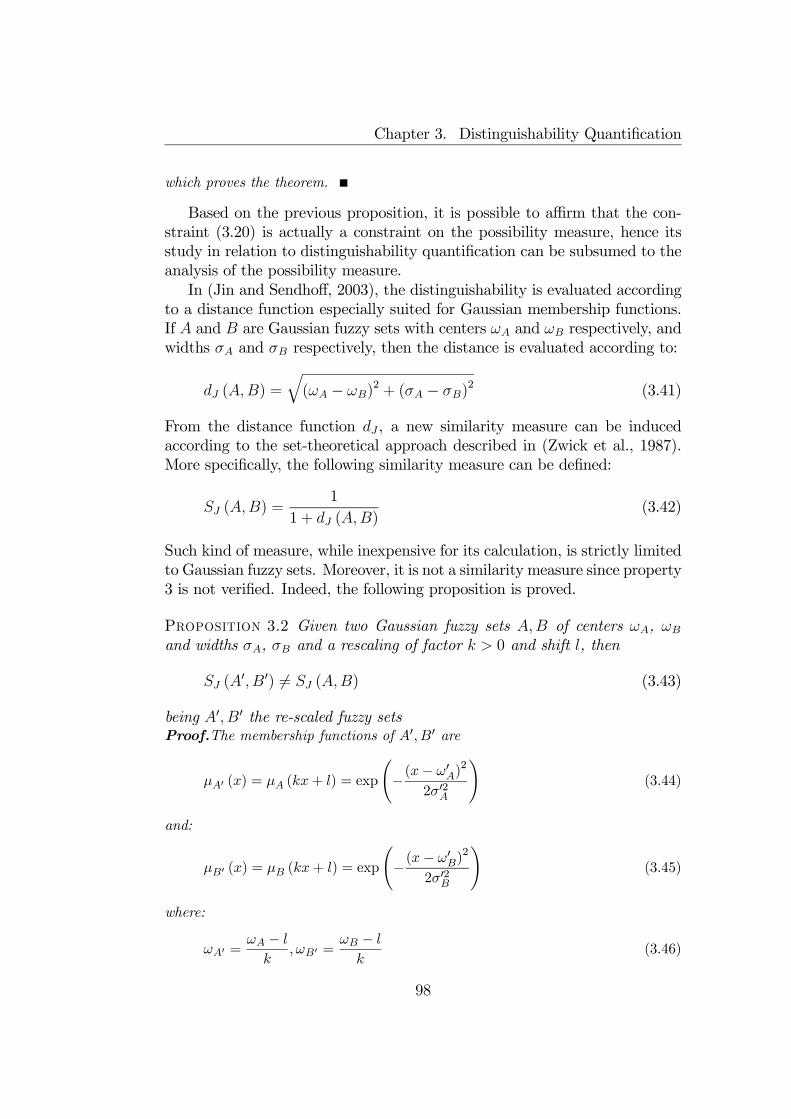
Chapter 3. Distinguishability Quantification
which proves the theorem.
Based on the previous proposition, it is possible to affirm that the con-straint (3.20) is actually a constraint on the possibility measure, hence itsstudy in relation to distinguishability quantification can be subsumed to theanalysis of the possibility measure.In (Jin and Sendhoff, 2003), the distinguishability is evaluated according
to a distance function especially suited for Gaussian membership functions.If A and B are Gaussian fuzzy sets with centers ωA and ωB respectively, andwidths σA and σB respectively, then the distance is evaluated according to:
dJ (A,B) =
q(ωA − ωB)
2 + (σA − σB)2 (3.41)
From the distance function dJ , a new similarity measure can be inducedaccording to the set-theoretical approach described in (Zwick et al., 1987).More specifically, the following similarity measure can be defined:
SJ (A,B) =1
1 + dJ (A,B)(3.42)
Such kind of measure, while inexpensive for its calculation, is strictly limitedto Gaussian fuzzy sets. Moreover, it is not a similarity measure since property3 is not verified. Indeed, the following proposition is proved.
Proposition 3.2 Given two Gaussian fuzzy sets A,B of centers ωA, ωB
and widths σA, σB and a rescaling of factor k > 0 and shift l, then
SJ (A0, B0) 6= SJ (A,B) (3.43)
being A0, B0 the re-scaled fuzzy setsProof.The membership functions of A0, B0 are
µA0 (x) = µA (kx+ l) = exp
Ã−(x− ω0A)
2
2σ02A
!(3.44)
and:
µB0 (x) = µB (kx+ l) = exp
Ã−(x− ω0B)
2
2σ02B
!(3.45)
where:
ωA0 =ωA − l
k, ωB0 =
ωB − l
k(3.46)
98

3.3. Theorems about Similarity and Possibility measures
and
σ0A =σAk, σ0B =
σBk
(3.47)
As a consequence:
dJ¡A0, B0
¢=
dJ (A,B)
k(3.48)
and hence
SJ¡A0, B0
¢=
k
k + dJ (A,B)6= SJ (A,B) (3.49)
for k 6= 1.
This and other issues are faced in (Guillaume and Charnomordic, 2004),where a more sophisticated metric is adopted for fuzzy partitioning withsemantic constraints.
3.3 Theorems about Similarity and Possibil-ity measures
On the basis of the considerations discussed in the previous Section, thepossibility measure emerges as a potentially good candidate for distinguisha-bility quantification. The main advantage deriving from adopting possibilityconsists in a more efficient evaluation of distinguishability, which can be usedin on-line learning schemes. However, the adoption of possibility for quan-tifying distinguishability is consistent provided the existence of a monotonicrelation between possibility and similarity, i.e. a relation that assures lowgrades of similarity for small values of possibility and vice versa. Unfortu-nately, as previously showed in examples 3.1 and 3.2, such relation does notexist unless some restrictions are imposed on the involved fuzzy sets.To find a relationship between possibility and similarity, in this Section
it will be proved that the involved fuzzy sets must verify the following inter-pretability constraints:
• Normality;
• Convexity;
• Continuity.
99

Chapter 3. Distinguishability Quantification
The three above-mentioned constraints are widely used in interpretablefuzzy modeling, since usually fuzzy sets used in model design belong to spe-cific classes (such as triangular, Gaussian, trapezoidal, etc.) that fulfill allthe three properties. As a consequence, assuming the validity of the aboveproperties does not limit the subsequent analysis to any specific class of in-terpretable fuzzy model.Before enunciating the relation between similarity and possibility, two
technical lemmas are necessary to establish some useful properties of convexfuzzy sets, which will turn useful in the successive discussion.
Lemma 3.1 For any convex fuzzy set A there exists an element p ∈ U suchthat the membership function µA restricted to the sub-domain
UL = x ∈ U : x ≤ p (3.50)
is non-increasing. Similarly, the membership function µA restricted to thesub-domain
UR = x ∈ U : x ≥ p (3.51)
is non-decreasing.Proof.Let p ∈ argmax
x∈UµA (x) . Consider two points x1 < x2 ≤ p and the corre-
sponding membership values α1 = µA (x1) and α2 = µA (x2). By definition ofconvexity, α2 ≥ min µA (p) , α1 = α1. Hence, the membership function µA isnon-decreasing in UL. With the same procedure, it can be proved that µA is non-increasing in UR.
Lemma 3.2 Let A and B be two continuous convex normal fuzzy sets withpA ∈ argmaxµA and pB ∈ argmaxµB such that pA < pB. Then, thereexists a point between pA and pB whose membership degree (both on A andB) corresponds to the possibility measure between A and B:
Π (A,B) = ϑ→ ∃x ∈ [pA, pB] : µA (x) = µB (x) = ϑ (3.52)
Proof.By definition of possibility (3.11):
ϑ = supminx∈U
µA (x) , µB (x) (3.53)
Because of continuity of fuzzy set A, and by Weierstrass theorem, the range of µAin the interval [pA, pB] is a closed interval [mA, 1]. Similarly, the range of µB inthe same interval is [mB, 1]. Let be:eϑ = supmin
x∈[pA,pB ]µA (x) , µB (x) (3.54)
100

3.3. Theorems about Similarity and Possibility measures
Let ex ∈ [pA, pB] such that min µA (ex) , µB (ex) = eϑ. Without loss of general-ity, suppose that µA (ex) = eϑ < 1. Because of convexity of A, then ∀x : pA ≤x < ex → µA (x) > eϑ. As a consequence µB (ex) ≥ eϑ. If µB (ex) > eϑ, then forany ∆ex > 0 sufficiently small, µB (ex−∆ex) > eϑ and µA (ex−∆ex) > eϑ. Thus,min µA (ex−∆ex) , µB (ex−∆ex) > eϑ and (3.54) would be invalidated. As a con-sequence, µB (ex) = µA (ex) = eϑ. In the specific case of eϑ = 1 , the equality of thetwo membership values is trivial.Suppose now, ab absurdo, that the possibility measure ϑ is different from eϑ, i.e.ϑ > eϑ (the case ϑ < eϑ is impossible by definition of possibility measure). Twocases can be considered:
(i) ∃xϑ < pA : min µA (x) , µB (x) = ϑ (3.55)
(ii) ∃xϑ > pB : min µA (x) , µB (x) = ϑ (3.56)
We consider first case (i). Then, xϑ < ex ≤ pB and µB (xϑ) = ϑ > eϑ = µB (ex).But since B is convex, by Lemma 3.1 xϑ < ex ≤ pB → µB (xϑ) = ϑ ≤ µB (ex) = eϑ.This is a contradiction, thus, ϑ = eϑ. Case (ii) is symmetrical to case (i).The last lemma states that for convex, continuous and normal fuzzy sets,
the “intersection point” of the fuzzy membership functions µA and µB layingbetween the modal values of A and B determines the possibility value (seefig. 3.4). In this way, the analysis can be limited to the interval between themodal values of the two fuzzy sets, thus simplifying further considerationson relating possibility and similarity.Now it is possible to establish an important relation between possibility
and similarity with the following theorem.
Theorem 3.1 Let A and B be two fuzzy sets that are continuous, normaland convex. Let pA ∈ argmaxµA, pB ∈ argmaxµB and suppose pA < pB.Let ϑ = Π (A,B) and xϑ ∈ [pA, pB] such that µA (xϑ) = µB (xϑ) = ϑ. Inaddition, suppose that:
∀x ∈ ]pA, xϑ[ : d2µAdx2
(x) ≤ 0 (3.57)
and:
∀x ∈ ]xϑ, pB[ : d2µBdx2
(x) ≤ 0 (3.58)
Then, the similarity between A and B is upper-bounded by:
S (A,B) ≤ Smax =2ϑ
r + 2ϑ− rϑ(3.59)
101
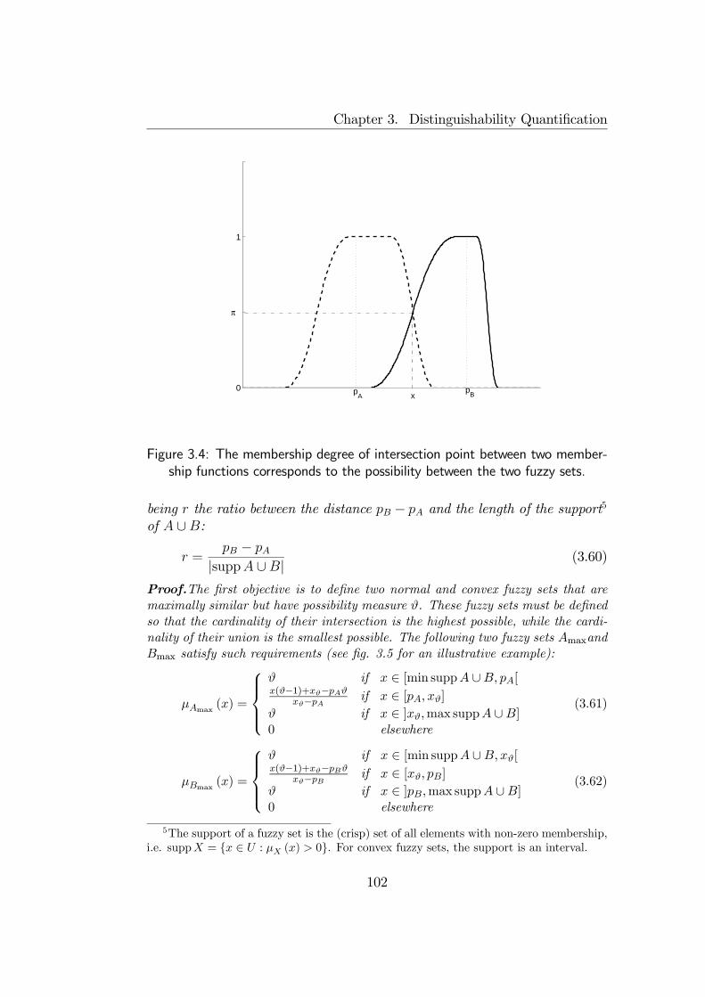
Chapter 3. Distinguishability Quantification
0
1
pA
pB
π
x
Figure 3.4: The membership degree of intersection point between two member-ship functions corresponds to the possibility between the two fuzzy sets.
being r the ratio between the distance pB − pA and the length of the support5
of A ∪B:r =
pB − pA|suppA ∪B| (3.60)
Proof.The first objective is to define two normal and convex fuzzy sets that aremaximally similar but have possibility measure ϑ. These fuzzy sets must be definedso that the cardinality of their intersection is the highest possible, while the cardi-nality of their union is the smallest possible. The following two fuzzy sets AmaxandBmax satisfy such requirements (see fig. 3.5 for an illustrative example):
µAmax (x) =
ϑ if x ∈ [min suppA ∪B, pA[x(ϑ−1)+xϑ−pAϑ
xϑ−pA if x ∈ [pA, xϑ]ϑ if x ∈ ]xϑ,max suppA ∪B]0 elsewhere
(3.61)
µBmax (x) =
ϑ if x ∈ [min suppA ∪B, xϑ[x(ϑ−1)+xϑ−pBϑ
xϑ−pB if x ∈ [xϑ, pB]ϑ if x ∈ ]pB,max suppA ∪B]0 elsewhere
(3.62)
5The support of a fuzzy set is the (crisp) set of all elements with non-zero membership,i.e. suppX = x ∈ U : µX (x) > 0. For convex fuzzy sets, the support is an interval.
102

3.3. Theorems about Similarity and Possibility measures
A B
pA pB
π
xπ
AmaxBmax
Figure 3.5: Example of fuzzy sets with maximal similarity for a given possibilitymeasure
The membership functions so defined are such that intersection and union coin-cide in all the support except the interval [pA, pB], while within such interval themembership functions have null second derivative. As a consequence, any coupleof fuzzy sets A and B satisfying the hypothesis will have:
∀x ∈ [pA, xϑ] : µA (x) ≥ µAmax (x) (3.63)
and
∀x ∈ [xϑ, pB] : µB (x) ≥ µBmax (x) (3.64)
In this way, the cardinality of the intersection fuzzy set is minimized while theunion is maximized. More specifically, the intersection of the two fuzzy sets hasthe following membership function:
µAmax∩Bmax (x) =
½ϑ if x ∈ suppA ∪B0 elsewhere
(3.65)
The union of the two fuzzy sets has the following membership function:
µAmax∪Bmax (x) =
ϑ if x ∈ [min suppA ∪B, pA[x(ϑ−1)+xϑ−pAϑ
xϑ−pA if x ∈ [pA, xϑ]x(ϑ−1)+xϑ−pBϑ
xϑ−pB if x ∈ [xϑ, pB]ϑ if x ∈ ]pB,max suppA ∪B]0 elsewhere
(3.66)
The similarity of the two fuzzy sets is:
S (Amax, Bmax) =|Amax ∩Bmax||Amax ∪Bmax| =
ϑ |suppA ∪B|ϑ |suppA ∪B|+ 1
2 (1− ϑ) (pB − pA)(3.67)
103
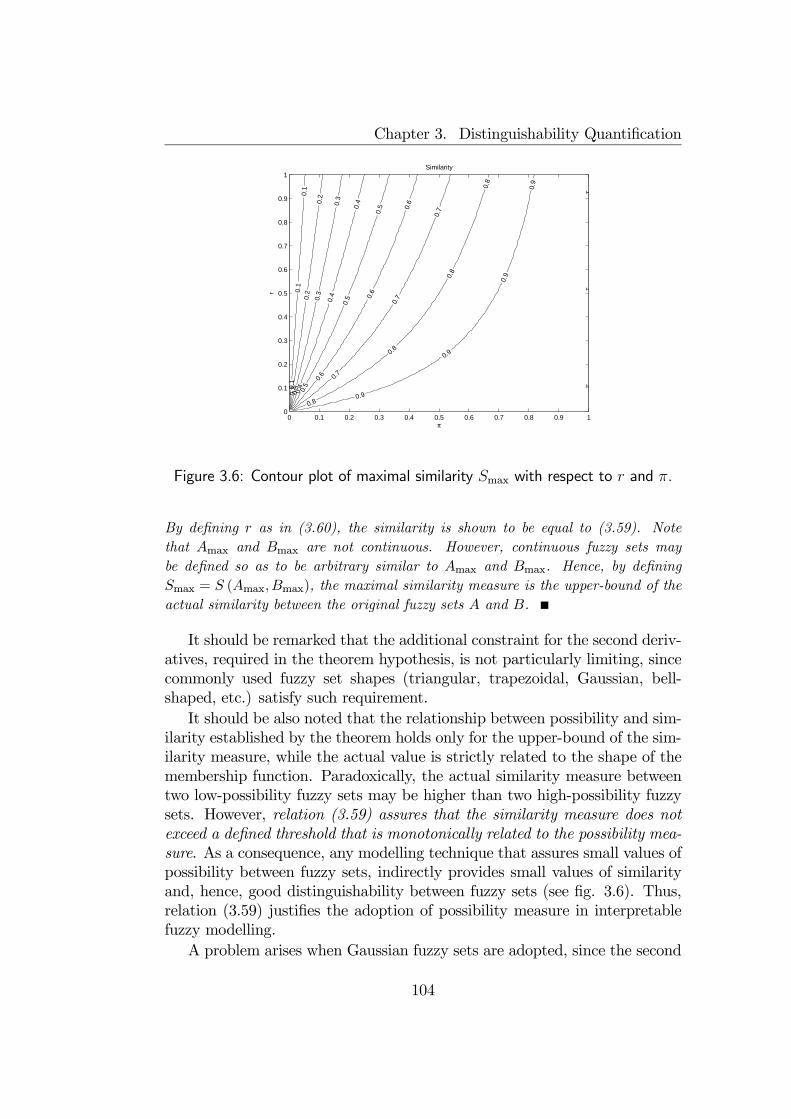
Chapter 3. Distinguishability Quantification
0 0.1 0.2 0.3 0.4 0.5 0.6 0.7 0.8 0.9 10
0.1
0.2
0.3
0.4
0.5
0.6
0.7
0.8
0.9
1
π
r
Similarity
0.1
0.1
0.1
0.2
0.2
0.2
0.3
0.3
0.3
0.4
0.4
0.4
0.5
0.5
0.5
0.6
0.6
0.6
0.7
0.7
0.7
0.8
0.8
0.8
0.8
0.9
0.9
0.9
0.9
11
1
Figure 3.6: Contour plot of maximal similarity Smax with respect to r and π.
By defining r as in (3.60), the similarity is shown to be equal to (3.59). Notethat Amax and Bmax are not continuous. However, continuous fuzzy sets maybe defined so as to be arbitrary similar to Amax and Bmax. Hence, by definingSmax = S (Amax, Bmax), the maximal similarity measure is the upper-bound of theactual similarity between the original fuzzy sets A and B.
It should be remarked that the additional constraint for the second deriv-atives, required in the theorem hypothesis, is not particularly limiting, sincecommonly used fuzzy set shapes (triangular, trapezoidal, Gaussian, bell-shaped, etc.) satisfy such requirement.It should be also noted that the relationship between possibility and sim-
ilarity established by the theorem holds only for the upper-bound of the sim-ilarity measure, while the actual value is strictly related to the shape of themembership function. Paradoxically, the actual similarity measure betweentwo low-possibility fuzzy sets may be higher than two high-possibility fuzzysets. However, relation (3.59) assures that the similarity measure does notexceed a defined threshold that is monotonically related to the possibility mea-sure. As a consequence, any modelling technique that assures small values ofpossibility between fuzzy sets, indirectly provides small values of similarityand, hence, good distinguishability between fuzzy sets (see fig. 3.6). Thus,relation (3.59) justifies the adoption of possibility measure in interpretablefuzzy modelling.A problem arises when Gaussian fuzzy sets are adopted, since the second
104

3.3. Theorems about Similarity and Possibility measures
derivatives of the respective membership functions may not be negative asrequested by the theorem. In order to satisfy the theorem hypothesis, it isnecessary that the intersection point between two Gaussian fuzzy set must laybetween the prototype and the inflection point of each membership function.To guarantee this condition, the possibility threshold should not be less than6
e−1/2 ≈ 0.606 53. However, a specific analysis can be made for Gaussianfuzzy sets, which shows that possibility and similarity are still monotonicallyrelated. Indeed, the following proposition can be proved.
Proposition 3.3 Let A and B be two Gaussian fuzzy sets with same width.If the possibility value between A and B is ϑ then their similarity measure is:
S (A,B) =1− erf ¡√− lnϑ¢1 + erf
¡√− lnϑ¢ (3.68)
where:
erf (x) =2√π
Z x
0
e−t2
dt (3.69)
Proof.Let ωA and ωB be the centers of the fuzzy sets A and B respectively. With-out loss of generality, it can be assumed ωA ≤ ωB. Let σ > 0 be the common widthof the two fuzzy sets. By lemma 3.2, it is possible to state that there exists a pointxϑ ∈ [ωA, ωB] such that:
µA (xϑ) = ϑ = µB (xϑ) (3.70)
Moreover, in example 2.2 (page 32) it has been proved that the intersection pointbetween two fuzzy sets of equal width is unique. As a consequence, the cardinalityof the intersection between the fuzzy sets A and B is the area depicted in fig 3.7.The expression for the cardinality of the intersection between A and B is therefore:
|A ∩B| =ZRmin µA (x) , µB (x) dx =
Z xϑ
−∞µB (x) dx+
Z +∞
xϑ
µA (x) dx (3.71)
For the sake of simplicity, it is assumed that the Universe of Discourse coincidedwith the real line R. Since each membership function is symmetrical w.r.t. itscenter, and since the membership function µB can be viewed as a horizontal trans-lation of µA of length ωB − ωA, it is possible to simplify the previous relation inthe following:
|A ∩B| = 2Z +∞
xϑ
µA (x) dx (3.72)
6Note that this value is stable against possible variations in the definition of Gaussianmembership functions. Indeed, it is easy to prove that the indicated possibility threshold
is constant for any membership function of the form exp³− (x− ω)2 /aσ2
´with a > 0.
105
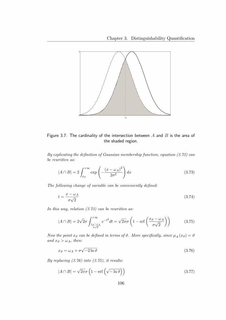
Chapter 3. Distinguishability Quantification
0
1
xϑ
Figure 3.7: The cardinality of the intersection between A and B is the area ofthe shaded region.
By explicating the definition of Gaussian membership function, equation (3.72) canbe rewritten as:
|A ∩B| = 2Z +∞
xϑ
exp
Ã−(x− ωA)
2
2σ2
!dx (3.73)
The following change of variable can be conveniently defined:
t =x− ωA
σ√2
(3.74)
In this way, relation (3.73) can be rewritten as:
|A ∩B| = 2√2σ
Z +∞
xϑ−ωAσ√2
e−t2dt =
√2πσ
µ1− erf
µxϑ − ωA
σ√2
¶¶(3.75)
Now the point xϑ can be defined in terms of ϑ. More specifically, since µA (xϑ) = ϑand xϑ > ωA, then:
xϑ = ωA + σ√−2 lnϑ (3.76)
By replacing (3.76) into (3.75), it results:
|A ∩B| =√2πσ
³1− erf
³√− lnϑ´´ (3.77)
106
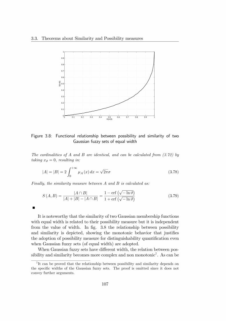
3.3. Theorems about Similarity and Possibility measures
0 0.1 0.2 0.3 0.4 0.5 0.6 0.7 0.8 0.9 10
0.1
0.2
0.3
0.4
0.5
0.6
0.7
0.8
0.9
1
Π(A,B)
S(A
,B)
Figure 3.8: Functional relationship between possibility and similarity of twoGaussian fuzzy sets of equal width
The cardinalities of A and B are identical, and can be calculated from (3.72) bytaking xϑ = 0, resulting in:
|A| = |B| = 2Z +∞
0µA (x) dx =
√2πσ (3.78)
Finally, the similarity measure between A and B is calculated as:
S (A,B) =|A ∩B|
|A|+ |B|− |A ∩B| =1− erf ¡√− lnϑ¢1 + erf
¡√− lnϑ¢ (3.79)
It is noteworthy that the similarity of two Gaussian membership functionswith equal width is related to their possibility measure but it is independentfrom the value of width. In fig. 3.8 the relationship between possibilityand similarity is depicted, showing the monotonic behavior that justifiesthe adoption of possibility measure for distinguishability quantification evenwhen Gaussian fuzzy sets (of equal width) are adopted.When Gaussian fuzzy sets have different width, the relation between pos-
sibility and similarity becomes more complex and non monotonic7. As can be
7It can be proved that the relationship between possibility and similarity depends onthe specific widths of the Gaussian fuzzy sets. The proof is omitted since it does notconvey further arguments.
107
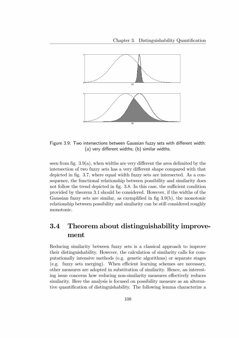
Chapter 3. Distinguishability Quantification
0
1
(a)
0
1
(b)
Figure 3.9: Two intersections between Gaussian fuzzy sets with different width:(a) very different widths; (b) similar widths.
seen from fig. 3.9(a), when widths are very different the area delimited by theintersection of two fuzzy sets has a very different shape compared with thatdepicted in fig. 3.7, where equal width fuzzy sets are intersected. As a con-sequence, the functional relationship between possibility and similarity doesnot follow the trend depicted in fig. 3.8. In this case, the sufficient conditionprovided by theorem 3.1 should be considered. However, if the widths of theGaussian fuzzy sets are similar, as exemplified in fig 3.9(b), the monotonicrelationship between possibility and similarity can be still considered roughlymonotonic.
3.4 Theorem about distinguishability improve-ment
Reducing similarity between fuzzy sets is a classical approach to improvetheir distinguishability. However, the calculation of similarity calls for com-putationally intensive methods (e.g. genetic algorithms) or separate stages(e.g. fuzzy sets merging). When efficient learning schemes are necessary,other measures are adopted in substitution of similarity. Hence, an interest-ing issue concerns how reducing non-similarity measures effectively reducessimilarity. Here the analysis is focused on possibility measure as an alterna-tive quantification of distinguishability. The following lemma characterize a
108
3.4. Theorem about distinguishability improvement
wide class of possibility-reducing procedures.
Lemma 3.3 Let A and B two fuzzy sets defined on the Universe of Dis-course U , which are continuous normal and convex. Let pA ∈ argmaxµA,pB ∈ argmaxµB and suppose pA < pB. Let Φ : F (U) → F (U) be a trans-formation such that B0 = Φ (B) is a continuous, normal and convex fuzzyset, and ∀x ∈ U : x ≤ pB → µB0 (x) ≤ µB (x). Then,
Π (A,B0) ≤ Π (A,B) (3.80)
Conversely, if B0 is such that ∀x ∈ U : x ≤ pB → µB0 (x) ≥ µB (x), then
Π (A,B0) ≥ Π (A,B) (3.81)
Proof.We consider only the first thesis (3.80), because the other can be provedsimilarly. Let ϑ be the possibility measure Π (A,B). In force of Lemma 3.2,
∃xϑ ∈ [pA, pB] : µA (x) = µB (x) = ϑ (3.82)
By hypothesis, µB0 (xϑ) ≤ ϑ, and re-applying Lemma 3.2 to A and B0, it can bestated that:
∃x0 ∈ [pA, pB0 ] : µA¡x0¢= µB0
¡x0¢= Π
¡A,B0
¢= ϑ0 (3.83)
where pB0 ∈ argmaxµB0. If µB0 (xϑ) < µB (xϑ), then ∀x00 < xϑ : µA (x00) ≥ ϑ ∧
µB0 (x00) ≤ µB0 (xϑ) < ϑ. Hence, ∀x00 < xϑ : µA (x
00) 6= µB (x00). As a consequence,
x0 ≥ xϑ. In such case, ϑ0 = µA (x0) ≤ µA (x) = ϑ, i.e. Π (A,B0) ≤ Π (A,B).
Two very common examples of transformations satisfying the lemma’shypothesis are the translation (µB0 (x) = µB (x− x0) , x0 > 0) and the con-traction (µB0 (x) = µB (x)
p , p > 1) of the membership function. Such trans-formations can be effectively used to reduce possibility between two fuzzysets, but in order to establish whether such transformations also reduce simi-larity an additional condition must be introduced, as proved in the followingtheorem.
Theorem 3.2 Any transformation Φ : F (U)→ F (U) such that B0 = Φ (B)preserves lemma 3.3 hypothesis and additionally
r0 =pB0 − pA
|suppA ∪B0| ≥pB − pA
|suppA ∪B| = r (3.84)
produces a decrease of the maximal similarity Smax.
109
Chapter 3. Distinguishability Quantification
Proof.The function Smax (ϑ, r) = 2ϑr+2ϑ−rϑ given in (3.59) is continuous and deriv-
able for every ϑ ∈ [0, 1]. Its derivative is:∂Smax∂ϑ
=2r
(r + 2ϑ− rϑ)2(3.85)
Since the ratio r is always positive, Smax is monotonically decreasing as ϑ de-creases, for a fixed ratio r. However, the new fuzzy set B0 may determine a differ-ent ratio r0 different from r. The directional derivative of Smax w.r.t. the direction(∆ϑ,∆r) is:
dSmaxd (∆ϑ,∆r)
= ∇Smax · (∆ϑ,∆r)k(∆ϑ,∆r)k =2r∆ϑ+ 2ϑ (ϑ− 1)∆r
k(∆ϑ,∆r)k (r + 2ϑ− rϑ)2(3.86)
Such derivative is negative (i.e. Smax is decreasing) when:
∆r >2r∆ϑ
2ϑ (1− ϑ)(3.87)
For ∆ϑ < 0 (reduced possibility), the second member of (3.87) is negative, henceany transformation that does not reduce the ratio (∆r = r0− r ≥ 0) will effectivelyreduce the maximal possibility Smax.
As a corollary of the theorem, every method aimed to reduce possibilityactually reduces (maximal) similarity, thus improving distinguishability. Inthis sense, the adoption of possibility as a measure of distinguishability isfully justified. The additional constraint required in the corollary (the ratior must not decrease) is always fulfilled by any translation that lengthensthe distance between the prototypes, as well as by contractions. However,attention must be paid for those transformation that reduce the support, forwhich the relation (3.87) must be carefully taken into account.
3.5 Final remarks
In this Chapter, it has been shown that possibility is both an effective andcomputationally efficient measure to quantify distinguishability, an impor-tant constraint for interpretable fuzzy modelling. Indeed, while similaritycan be considered as the most representative measure for distinguishabilityof fuzzy sets, it has been proved that under mild conditions (always satisfiedby interpretable fuzzy sets) possibility and similarity are related monotoni-cally, so that small values of possibility imply small values of similarity. Theadded values of possibility measures are its sound semantic meaning and thecomputationally efficiency of the calculation procedure. As a matter of fact,in most cases possibility measure can be expressed analytically in terms of
110

3.5. Final remarks
fuzzy sets parameters, so it can be used in many learning schemes withoutresorting computationally intensive algorithms.
111

Chapter 3. Distinguishability Quantification
112

Chapter 4
Interface Optimality
4.1 Introduction
Frames of Cognition are employed in fuzzy modelling to provide a granulatedview of a simple (i.e. one-dimensional) attribute by means of interpretablefuzzy sets that can be designated by semantically sound linguistic labels.Frames of Cognition are at the basis for the definition of more complex in-formation granules that relate different attributes so as to express knowledgeand perform approximate reasoning.From a functional point of view, Frames of Cognition can be regarded
as mappings that convert an external representation of information to aninternal one (or vice versa), which is suited to the information processing thatis carried out within a fuzzy model. For such reason, Frames of Cognitionare parts of the so-called “Input Interfaces” and “Output Interfaces”, whichare — along with the “Processing Module” — the main functional blocks mostfuzzy models.The role of the Input Interface consists in the conversion of informa-
tion coming from the environment in an internal format acceptable by theProcessing Module. Symmetrically, the Output Interface transforms infor-mation coming from the processing module into a suited external representa-tion to be used in the environment. The information transformation from theexternal to the internal representation can be carried out through a match-ing procedure employing a family of referential fuzzy sets that belong tosome Frame of Cognition. Specifically, the Input Interface provides a map-ping from numerical data into a structure of fuzzy membership values, whilethe Output Interface transforms such structures into numerical results. Al-though the roles of the input and output interfaces are quite different, bothof them share the same framework as being based on Frames of Cognition
113
Chapter 4. Interface Optimality
(de Oliveira, 1993; de Oliveira, 1995; Pedrycz and de Oliveira, 1996).As it is widely recognized that the impact of the performance of fuzzy
models heavily depends on the input/output interfaces, a careful design ofsuch functional blocks is crucial for the overall quality of the fuzzy models.With this purpose, several criteria have been proposed in order to guar-antee well-designed interfaces in terms of two main factors: the semanticintegrity of the modeled linguistic terms and the precise representation ofuncertain input data (Valente de Oliveira, 1999a; Pedrycz, 1996b). In partic-ular, precise representation can be guaranteed by the so-called “InformationEquivalence Criterion” (Pedrycz and de Oliveira, 1996), also called “Anti-fuzzy-aliasing Condition” (de Oliveira, 1996) or “Error-free Reconstruction”(Pedrycz, 1994). According to the Information Equivalence Criterion, aninterface should preserve the information coming into (or outcoming from)the processing block by converting it into a relevant internal representationappropriate for further processing. An interface that satisfies the Informa-tion Equivalence Criterion is also called “Optimal Interface” (de Oliveira,1996). Using optimal interfaces, it can be proved that each external datumhas its own internal representation, and referential fuzzy sets cover the entireUniverse of Discourse (Valente de Oliveira, 1998).In interpretable fuzzy modelling, optimal Input Interfaces are important
because they provide for a precise internal representation of the informa-tion coming from the environment. More specifically, for different inputs,an optimal Input Interface returns different representations that are furtherprocessed by the Processing Module. In case of sub-optimality, there wouldexists two or more inputs for which the same representation is provided bythe Input Interface. In this way, the inputs would processed exactly in thesame way: they would be indistinguishable even though they are different.But often fuzzy models are used because their internal knowledge is definedby formal concepts (i.e. the information granules) that are always verifiedto a degree. Therefore, it could be expected that different inputs verify con-cepts to different degrees, in the same way humans perceive different stimuliwith different intensities. As a consequence, sub-optimality of Input Inter-faces could make fuzzy models too approximative to be acceptable in certainapplicative contextsConversely, optimal Output Interfaces provide for an invertible represen-
tation of the inference process carried out by the Processing Module. In thecontext of interpretable fuzzy modelling, this means that the output of themodel could be re-fuzzified to yield the same fuzzy representation providedby the Processing Module. Such representation is a structure of truth de-grees, usually consequence degrees of a list of rules. Therefore, the outputof the model would verify the consequent of each rule with the same degree
114
4.1. Introduction
provided by the Processing Module. This is exactly what is required by afully interpretable inference process: if the strength of a rule is high (resp.low), it is expected that the inferred output verifies the rule consequent witha high (resp. low) degree1. In this sense, optimality of the Output Interfaceis a necessary condition to guarantee that the output provided by the modelis in strict correspondence with the conclusion inferred by the ProcessingModule.Optimal Interfaces have been extensively studied in the context of Frames
of Cognition defined by triangular fuzzy sets (de Oliveira, 1993; de Oliveira,1995; Pedrycz, 1994; Pedrycz and de Oliveira, 1996), but little attention hasbeen paid to interfaces based on fuzzy sets of different shapes, such as trape-zoidal, Gaussian, bell-shaped, etc. (Zimmermann, 2001). Moreover, someauthors are skeptical concerning the real effectiveness of triangular fuzzy setsin solving modeling problems (see for example (Mitaim and Kosko, 2001)).Conversely, convex fuzzy sets are regarded as a promising class of fuzzy setsto guarantee interface optimality (de Oliveira, 1995). Hence, the issue ofoptimality of interfaces based on different shapes of fuzzy sets should beaddressed.In this Chapter, it is proved that optimality of Input Interfaces can be
guaranteed for a wide class of fuzzy sets, provided that mild conditions aresatisfied. In particular, after the definition of two main classes of fuzzysets, namely “strictly bi-monotonic” fuzzy sets and “loosely bi-monotonic”fuzzy sets, two theorems are proved. The first theorem proves that optimalinterfaces are always guaranteed for strictly bi-monotonic fuzzy sets (e.g.Gaussian fuzzy sets), provided that weak conditions hold. The second theo-rem states that optimality is guaranteed for loosely bi-monotonic fuzzy sets(e.g. triangular and convex fuzzy sets in general) if stronger conditions hold.The theorems provide sufficient conditions for optimality for a wide class offuzzy sets, including convex fuzzy sets, so that their results can be useful ina broad range of fuzzy modeling contexts.Such theoretical results, derived for Input Interfaces, are not applicable to
Output Interfaces. Indeed, while Input Interfaces are usually implementedby a matching mechanism that derives membership values from numericalvalues, Output Interfaces are generally defined by an aggregation operationthat can easily hamper the optimality condition. Nevertheless, the Infor-mation Equivalence Criterion should be taken into account in the design ofOutput Interfaces, since it is a necessary condition to define transparent andaccurate models. For such reason, a different optimality criterion is pro-posed, which leads to the definition of an Optimality Degree that measures
1Assuming a conjunctive interpretation of rules, see §2.6
115

Chapter 4. Interface Optimality
Figure 4.1: The three functional blocks of a Fuzzy Model
the quality of a fuzzy Output Interface. According to such criterion, differ-ent Output Interfaces can be compared and their quality ranked accordingto their optimality.The Chapter is organized as follows. Section 4.2 provides a formal de-
scription of Input and Output Interfaces. In Section 4.3, the optimality ofInput Interfaces is addressed: the class of bi-monotonic fuzzy sets is definedand two theorems on optimality conditions for bi-monotonic fuzzy sets areproved. In Section 4.4, the optimality of Output Interfaces is discussed, andthe Optimality Degree is introduced. Also, an illustrative example is pre-sented to show how the defined optimality degree can be conveniently usedto highlight quality variations attained by different output interfaces. Finally,in Section 4.5 some conclusions are drawn.
4.2 Fuzzy Interfaces
A Fuzzy Model is typically composed of three main functional blocks (fig.4.1), namely the Input and the Output Interface communicating betweenthe modeling environment, and the processing module dedicated for fuzzycomputations. In the following,he role of each functional block is brieflydescribed along with the basic terminology.
4.2.1 Input Interface
The role of the Input Interface is to transform the data about a certainapplication from the usual numerical level into the linguistic level. In otherwords, an Input Interface provides a fuzzy discretization of external data bymeans of a family of Kx reference fuzzy sets. For nx-dimensional data ofdomain X ⊆ Rnx, the (multidimensional) Input Interface can be formalizedas follows:
= : X ⊂ Rnx → [0, 1]Kx (4.1)
116
4.2. Fuzzy Interfaces
such that:
∀x ∈ X : = (x) = [Ai (x)]i=1,2,...Kx(4.2)
where Ai (x) is the membership degree of the i-th reference fuzzy set. Itshould be remarked that the definition of Input Interfaces can be extendedto deal with fuzzy inputs, as remarked in (Pedrycz and de Oliveira, 1996),but in such case it is impossible to perfectly reconstruct inputs when onlymembership values are given (see (Pedrycz and Gomide, 1998) for a completeproof).Usually, in interpretable fuzzy models, an Input Interface is composed of
several one-dimensional Input Interfaces defined by Frames of Cognition. Insuch a case, the (multidimensional) Input Interface is defined as follows:
∀x ∈ X ⊆ Rnx : = (x) = £=(j) (xj)¤j=1,2,...nx (4.3)
being x = [x1, x2, . . . , xnx] and =(j) the j-th one-dimensional Input Interfacewhich is in the form:
=(j) : X(j) ⊆ R→ [0, 1]K(j)x , j = 1, 2, . . . nx (4.4)
Each one-dimensional Input Interface can be defined as the functionalcounterpart of a Frame of Cognition. Specifically, if for the j-th attributethe following Frame of Cognition is defined:
F(j) =U (j),F(j),¹(j),L(j), v(j)® (4.5)
being the family of fuzzy sets:
F(j) =nA(j)1 , A
(j)2 , . . . , A
(j)
K(j)x
o(4.6)
then, the j-th input interface is defined as:
=(j) (x) =³A(j)1 (x) , A
(j)2 (x) , . . . , A
(j)
K(j)x
(x)´
(4.7)
with the assumption that A(j)i ¹(j) A(j)i+1.
4.2.2 Processing Module
The outcome of the Input Interface is transformed into a structure of outputmembership degrees by the processing module, which is dedicated to allcomputations at a fuzzy level. From a functional point of view, the processingmodule can be formalized as follows:
P : [0, 1]Kx → [0, 1]Ky (4.8)
The processing module can be implemented in several forms, including fuzzyrelational calculus, fuzzy regression models and fuzzy neural networks (Pedrycz,1995).
117
Chapter 4. Interface Optimality
4.2.3 Output Interface
The role of the Output Interface (Output Interface) consists in transformingthe results produced by the processing module into a form acceptable by themodeling environment, which often calls for numerical values. Hence, suchtransformation completes a mapping from the linguistic to the numericallevel. From a functional point of view, the Output Interface can be formalizedas:
O : [0, 1]Ky → Rny (4.9)
For simplicity, it is assumed that ny = 1, i.e. the Output Interface pro-vides only a one-dimensional numerical value. The extension to multidi-mensional outputs is straightforward by considering ny Output Interfacesindependently.Generally, an Output Interface is characterized by a family of referential
fuzzy sets belonging to a related Frame of Cognition and the final numericaloutput is calculated by means of a defuzzification algorithm, which operatesby aggregating membership degrees coming from the processing module.Depending on the type of the fuzzy model, the Output Interface can be
very simple or quite complex. In Takagi-Sugeno Fuzzy Inference Systemswith rules of the following type:
IF x is A(r) THEN y = w(r) (4.10)
the Output Interface is defined as a weighted average formula:
OTS (πy) =
PKy
r=1 π(r)y · w(r)PKy
r=1 π(r)y
(4.11)
being πy =hπ(1)y , π
(2)y , . . . , π
(Ky)y
ithe vector of membership degrees provided
by the Processing Module, with π(r)y = A(r) (x). In a Mamdani Fuzzy Infer-
ence System with rules of the following type:
IF x is A(r) THEN y is B(r) (4.12)
the Output Interface derives, for each rule, a new fuzzy set as follows:
B(r) (y) = B(r) (y)⊗ π(r)y (4.13)
being ⊗ a t-norm like the minimum or the product operator. Then, all suchfuzzy sets are aggregated to form a unique fuzzy set:
B =
Ky[r=1
B(r) (4.14)
118

4.3. Theorems about optimality for Input Interfaces
centroid ey = RB(y)·y·dyRB(y)·dy
bisector ey s.t.R y−∞B (y) dy =
R +∞y
B (y) dy
mean of maxima (MOM) ey = φeM φ
|M | ,M = argmaxB
sup of maxima (SOM) ey = sup (argmaxB)inf of maxima (LOM) ey = inf (argmaxB)
Table 4.1: Some common defuzzification formulas
where the union operation can be computed by means of a t-conorm, likethe maximum or the probabilistic sum. Finally the aggregate fuzzy set B isreduced to a single numerical value y according to a defuzzification method,like those illustrated in table 4.1 (for a more complete review of defuzzifica-tion methods, see (Lee, 1990)). Hence, in case of Mamdani Fuzzy InferenceSystems, the Output Interface is implicitly defined by one of the above de-fuzzification formulas.
4.3 Theorems about optimality for Input In-terfaces
The idea behind the concept of optimal interface states that an error-freeconversion should exist when the values of a given numerical variable aretransformed in the internal representation, and vice versa. Hence, an InputInterface is defined as optimal if it is invertible, i.e. there exists a way toexactly determine the input value when the vector of membership degrees isgiven. Formally:
opt (=,X)⇔ ∃=−1 s.t.∀x ∈ X : =−1 (= (x)) = x (4.15)
The optimality condition of a multidimensional Input Interface defined asin (4.3) is met when all its composing one-dimensional Input Interfaces areoptimal.It should be remarked that this definition is slightly different from those
found in literature to characterize optimality (see, e.g., (Valente de Oliveira,1998; Valente de Oliveira, 1999a; Pedrycz, 1994)). Indeed, other authorsprovide a definition of optimality for a given couple of I/O interfaces, beingthe Output Interface the inverse function of the Input Interface. This inversefunction is usually defined by a defuzzification formula. Conversely, in (4.15)the inverse function of the Input Interface is not explicitly given, but it is sim-ply required to exist. In other words, such inverse function may not coincide
119
Chapter 4. Interface Optimality
with any known defuzzification method, but the definition still guaranteesthat no ambiguity is introduced in the conversion process performed by theInput Interface.In the design of an Input Interface, the optimality condition can be easily
guaranteed if the referential fuzzy sets are properly chosen. Here, a familyof fuzzy sets which guarantee optimality condition is characterized. Thisfamily embraces two classes of fuzzy sets, called bi-monotonic, that covermost types of fuzzy sets, including convex fuzzy sets. In the following, afterthe definition of the two classes of bi-monotonic fuzzy sets, namely strictlybi-monotonic fuzzy sets and loosely bi-monotonic fuzzy sets, two theoremsabout optimality condition are formulated and proved.
4.3.1 Bi-monotonic fuzzy sets
Definition 4.1 (bi-monotonic fuzzy sets) A one-dimensional fuzzy setA defined over the Universe of Discourse X ⊆ R is strictly bi-monotonic ifthere exists a prototype p ∈ X (i.e. A (p) = 1) such that the restrictions of themembership function2 A : X → [0, 1] to the sub-domains XL = X ∩ ]−∞, p]and XR = X ∩ [p,+∞[ are strictly monotonic. The fuzzy set A is (loosely)bi-monotonic if such restrictions are loosely monotonic. Of course, strictlybi-monotonic fuzzy sets are also loosely bi-monotonic. We will call the twoabove mentioned restrictions as AL (left restriction) and AR (right restric-tion).
Lemma 4.1 If A is (strictly/loosely) bi-monotonic, then the complement ofA (i.e. A (x) = 1−A (x)) is bi-monotonic.
Lemma 4.2 If A is strictly bi-monotonic, then ∀π ∈ [0, 1] : |A−1 (π)| ≤ 2,where A−1 (π) = x ∈ X|A (x) = π.Proof.If the range of the membership function of A is ρ (A) ⊆ [0, 1], then ∀π ∈[0, 1]− ρ (A) : A−1 (π) = ∅.Let p be a prototype of A. If π ∈ ρ (A), let:
A−1L (π) = x ∈ X ∩ ]−∞, p] |A (x) = π (4.16)
A−1R (π) = x ∈ X ∩ [p,+∞[ |A (x) = π (4.17)
Then¯A−1L (π)
¯ ≤ 1 because if ∃x1, x2 : x1 < x2 ∧ x1 ∈ A−1L (π) ∧ x2 ∈ A−1L (π),then ∃x1, x2 : x1 < x2 ∧ AL (x1) = AL (x2) that is, the left restriction AL
would not be strictly monotonic. The same is true for AR. As a consequence,A−1 (π) = A−1L (π) ∪A−1R (π)⇒ ¯
A−1 (π)¯ ≤ ¯A−1L (π)
¯+¯A−1R (π)
¯ ≤ 2.2Hereafter, the membership function of a fuzzy set A is denoted with the same symbol
A and not by µA, as in other chapters. This notation has been preferred for ease of reading.
120

4.3. Theorems about optimality for Input Interfaces
Corollary 4.1 If p is a prototype of A, then |A−1 (A (p))| = 1Proof.Note that p ∈ A−1L (A (p)) ∧ p ∈ A−1R (A (p)). If, ad absurdum,∃q s.t. p 6= q ∧ q ∈ A−1 (A (p)), then q ∈ A−1L (A (p)) ∨ q ∈ A−1R (A (p)), that is,¯A−1L (A (p))
¯> 1 ∨ ¯A−1R (A (p))
¯> 1. This is absurd.
Corollary 4.2 The support of a strictly bi-monotonic fuzzy set A definedover X is X − O, where O is a set with at most two elements, and can beeventually empty.
Lemma 4.3 Convex one-dimensional fuzzy sets are loosely bi-monotonic.Proof.Let A be a convex fuzzy set and p ∈ argmax
xeXA (x). Consider two points
x1, x2 ∈ X such that x1 < x2 < p and their respective membership degrees α1 =A(x1), α2 = A(x2). Because of convexity of A, α2 = A(x2) ≤ min A(x1), A (p) =A (x1) = α1, hence α1 6 α2. As a consequence, the restriction AL is looselymonotonic. Similarly, AR is loosely monotonic, so A is loosely bi-monotonic.
Corollary 4.3 Gaussian membership functions (and their complements)are strictly bi-monotonic. Triangular and trapezoidal membership functions(with their complements) are loosely bi-monotonic but, in general, not strictlybi-monotonic.
4.3.2 Optimality conditions
Two sufficient conditions of optimality are provided, for Input Interfacesbased on the two classes of bi-monotonic fuzzy sets (strictly and loosely).Such conditions are fulfilled if some mild constraints are satisfied.
Theorem 4.1 Let Φ = A1, A2, . . . , An be a family of one-dimensionalstrictly bi-monotonic fuzzy sets, with respective distinct prototypes p1 < p2 <· · · < pn such that ∀x ∈ X∃pi, pj : pi ≤ x ≤ pj.. Then, the correspondingInput Interface = (x) = (A1 (x) , A2 (x) , . . . , An (x)) is optimal.Proof.Let x ∈ X and = (x) = (π1, π2, . . . , πn). Let πi, πj be the values of(π1, π2, . . . , πn) corresponding to two fuzzy sets Ai, Aj ∈ Φ with prototypes pi, pjsuch that pi ≤ x ≤ pj. Then, A−1i (πi) ∩ A−1j (πj) = x. Indeed, suppose, adabsurdum, that A−1i (πi) ∩A−1j (πj) = y, z, with y < z (note thatx = y ∨ x = z, since x will always compare in the intersection by constructionof the defined sets). By Lemma 4.2, we have y ∈ A−1iL (πi) ∧ z ∈ A−1iR (πi) and,symmetrically, y ∈ A−1jL (πj) ∧ z ∈ A−1jR (πj). As a consequence, the prototypespi, pj are such that y ≤ pi < pj ≤ z, that is x ≤ pi < pj ∨ pi < pj ≤ x. This isabsurd. Since any two fuzzy sets are sufficient in uniquely determining the original
121
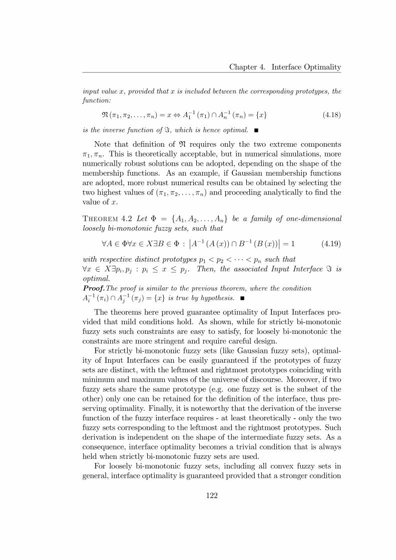
Chapter 4. Interface Optimality
input value x, provided that x is included between the corresponding prototypes, thefunction:
N (π1, π2, . . . , πn) = x⇔ A−11 (π1) ∩A−1n (πn) = x (4.18)
is the inverse function of =, which is hence optimal.Note that definition of N requires only the two extreme components
π1, πn. This is theoretically acceptable, but in numerical simulations, morenumerically robust solutions can be adopted, depending on the shape of themembership functions. As an example, if Gaussian membership functionsare adopted, more robust numerical results can be obtained by selecting thetwo highest values of (π1, π2, . . . , πn) and proceeding analytically to find thevalue of x.
Theorem 4.2 Let Φ = A1, A2, . . . , An be a family of one-dimensionalloosely bi-monotonic fuzzy sets, such that
∀A ∈ Φ∀x ∈ X∃B ∈ Φ :¯A−1 (A (x)) ∩B−1 (B (x))¯ = 1 (4.19)
with respective distinct prototypes p1 < p2 < · · · < pn such that∀x ∈ X∃pi, pj : pi ≤ x ≤ pj. Then, the associated Input Interface = isoptimal.Proof.The proof is similar to the previous theorem, where the conditionA−1i (πi) ∩A−1j (πj) = x is true by hypothesis.The theorems here proved guarantee optimality of Input Interfaces pro-
vided that mild conditions hold. As shown, while for strictly bi-monotonicfuzzy sets such constraints are easy to satisfy, for loosely bi-monotonic theconstraints are more stringent and require careful design.For strictly bi-monotonic fuzzy sets (like Gaussian fuzzy sets), optimal-
ity of Input Interfaces can be easily guaranteed if the prototypes of fuzzysets are distinct, with the leftmost and rightmost prototypes coinciding withminimum and maximum values of the universe of discourse. Moreover, if twofuzzy sets share the same prototype (e.g. one fuzzy set is the subset of theother) only one can be retained for the definition of the interface, thus pre-serving optimality. Finally, it is noteworthy that the derivation of the inversefunction of the fuzzy interface requires - at least theoretically - only the twofuzzy sets corresponding to the leftmost and the rightmost prototypes. Suchderivation is independent on the shape of the intermediate fuzzy sets. As aconsequence, interface optimality becomes a trivial condition that is alwaysheld when strictly bi-monotonic fuzzy sets are used.For loosely bi-monotonic fuzzy sets, including all convex fuzzy sets in
general, interface optimality is guaranteed provided that a stronger condition
122
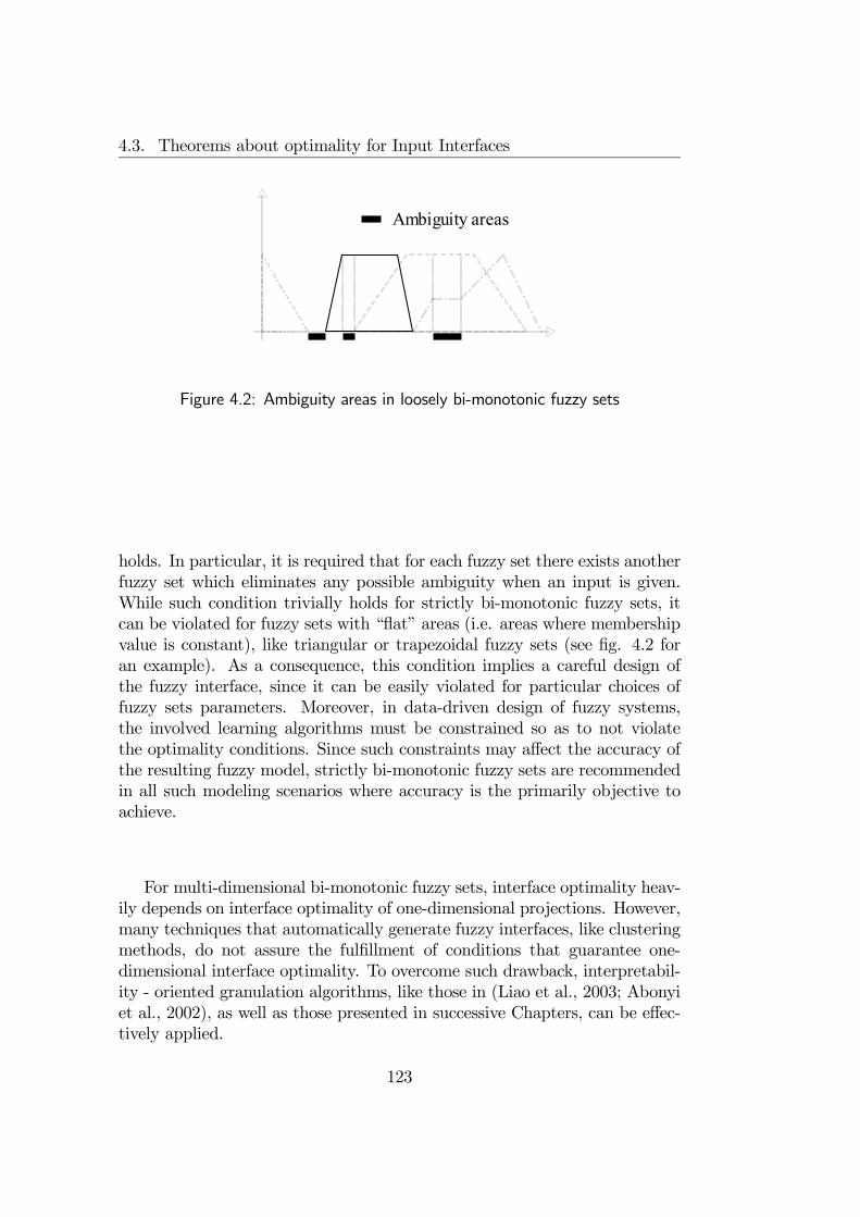
4.3. Theorems about optimality for Input Interfaces
Figure 4.2: Ambiguity areas in loosely bi-monotonic fuzzy sets
holds. In particular, it is required that for each fuzzy set there exists anotherfuzzy set which eliminates any possible ambiguity when an input is given.While such condition trivially holds for strictly bi-monotonic fuzzy sets, itcan be violated for fuzzy sets with “flat” areas (i.e. areas where membershipvalue is constant), like triangular or trapezoidal fuzzy sets (see fig. 4.2 foran example). As a consequence, this condition implies a careful design ofthe fuzzy interface, since it can be easily violated for particular choices offuzzy sets parameters. Moreover, in data-driven design of fuzzy systems,the involved learning algorithms must be constrained so as to not violatethe optimality conditions. Since such constraints may affect the accuracy ofthe resulting fuzzy model, strictly bi-monotonic fuzzy sets are recommendedin all such modeling scenarios where accuracy is the primarily objective toachieve.
For multi-dimensional bi-monotonic fuzzy sets, interface optimality heav-ily depends on interface optimality of one-dimensional projections. However,many techniques that automatically generate fuzzy interfaces, like clusteringmethods, do not assure the fulfillment of conditions that guarantee one-dimensional interface optimality. To overcome such drawback, interpretabil-ity - oriented granulation algorithms, like those in (Liao et al., 2003; Abonyiet al., 2002), as well as those presented in successive Chapters, can be effec-tively applied.
123
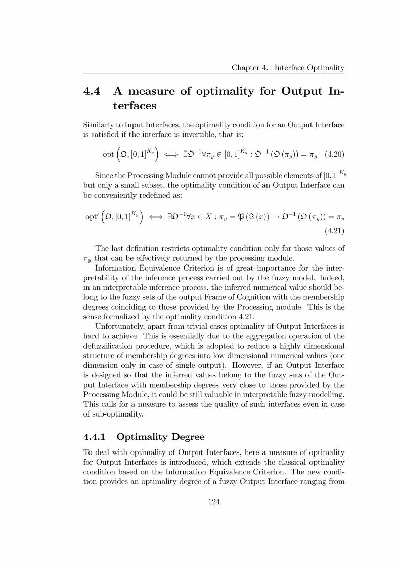
Chapter 4. Interface Optimality
4.4 A measure of optimality for Output In-terfaces
Similarly to Input Interfaces, the optimality condition for an Output Interfaceis satisfied if the interface is invertible, that is:
opt³O, [0, 1]Ky
´⇐⇒ ∃O−1∀πy ∈ [0, 1]Ky : O−1 (O (πy)) = πy (4.20)
Since the ProcessingModule cannot provide all possible elements of [0, 1]Ky
but only a small subset, the optimality condition of an Output Interface canbe conveniently redefined as:
opt0³O, [0, 1]Ky
´⇐⇒ ∃O−1∀x ∈ X : πy = P (= (x))→ O−1 (O (πy)) = πy
(4.21)
The last definition restricts optimality condition only for those values ofπy that can be effectively returned by the processing module.Information Equivalence Criterion is of great importance for the inter-
pretability of the inference process carried out by the fuzzy model. Indeed,in an interpretable inference process, the inferred numerical value should be-long to the fuzzy sets of the output Frame of Cognition with the membershipdegrees coinciding to those provided by the Processing module. This is thesense formalized by the optimality condition 4.21.Unfortunately, apart from trivial cases optimality of Output Interfaces is
hard to achieve. This is essentially due to the aggregation operation of thedefuzzification procedure, which is adopted to reduce a highly dimensionalstructure of membership degrees into low dimensional numerical values (onedimension only in case of single output). However, if an Output Interfaceis designed so that the inferred values belong to the fuzzy sets of the Out-put Interface with membership degrees very close to those provided by theProcessing Module, it could be still valuable in interpretable fuzzy modelling.This calls for a measure to assess the quality of such interfaces even in caseof sub-optimality.
4.4.1 Optimality Degree
To deal with optimality of Output Interfaces, here a measure of optimalityfor Output Interfaces is introduced, which extends the classical optimalitycondition based on the Information Equivalence Criterion. The new condi-tion provides an optimality degree of a fuzzy Output Interface ranging from
124

4.4. A measure of optimality for Output Interfaces
0 (excluded) to 1. The higher is such degree, the better is the quality ofthe interface. The maximal optimality degree corresponds to an optimal in-terface in the classical sense. Conversely, the lower is such degree the lessprecise is the conversion process performed by the fuzzy interface.To define the Optimality Degree of an Output Interface as in (4.9), a
related Input Interface is considered:
←−O : Rny → [0, 1]Ky (4.22)
The definition of←−O depends on the form of O. For Mamdani rules as in
(4.12),←−O is defined as follows:
∀y ∈ Rny :←−O (y) =
£B(r) (y)
¤r=1,2,...Ky
(4.23)
Once the Input Interface←−O has been derived, its optimality (in the clas-
sical sense) can be easily checked. If the related Input Interface←−O is optimal,
then O is defined as reversely optimal. Assuming that the Output Interfaceis reversely optimal, its optimality degree is computed as follows.
1. When an input x is presented to the fuzzy model, a structure of mem-bership degrees πy is computed by the Processing Module.
2. The vector πy is further processed by the Output Interface O, whichprovides a numerical value y.
3. Now the related Input Interface←−O is considered, and the structure of
membership values πy =←−O (y) is computed for the numerical value y.
4. If πy = πy, then the Output Interface is optimal for x. Conversely, themore πy is different from πy, the less optimal is the O-interface.
Given a distance measure d : [0, 1]Ky × [0, 1]Ky → R (e.g. the Euclideandistance), the Optimality Degree is hence defined as:
od (x) = exp (−d (πy, πy)) (4.24)
A value od (x) ≈ 1 means that the membership values provided by theProcessing Module can be reconstructed almost perfectly. When od (x) ≈ 1,the output y produced by the Output Interface belongs to the fuzzy sets ofthe output Frame of Cognition with membership degrees very close to thoseprovided by the Processing Module. Conversely, if od (x) ¿ 1, the inferred
125
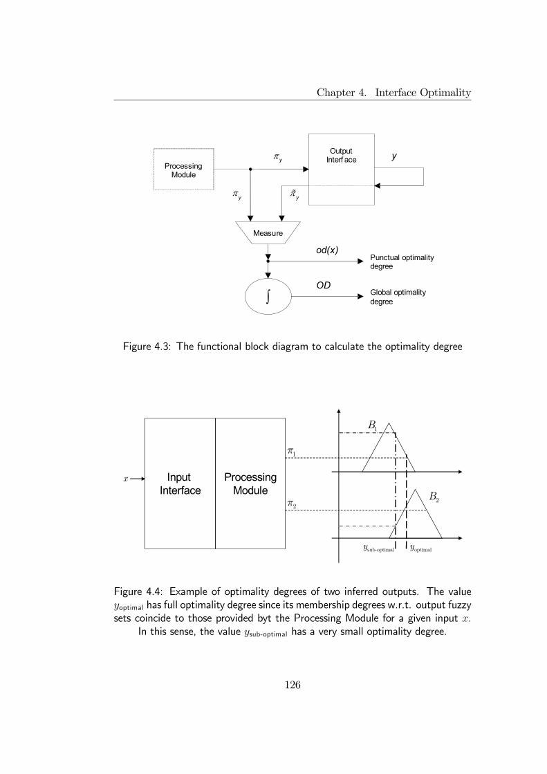
Chapter 4. Interface Optimality
Figure 4.3: The functional block diagram to calculate the optimality degree
1π
2π
1B
2B
optimaly
ProcessingModule
sub-optimaly
Input Interface
x
Figure 4.4: Example of optimality degrees of two inferred outputs. The valueyoptimal has full optimality degree since its membership degrees w.r.t. output fuzzysets coincide to those provided byt the Processing Module for a given input x.
In this sense, the value ysub-optimal has a very small optimality degree.
126
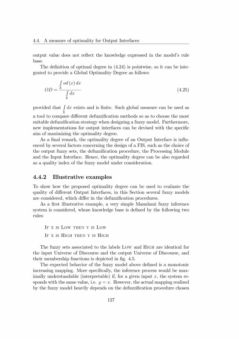
4.4. A measure of optimality for Output Interfaces
output value does not reflect the knowledge expressed in the model’s rulebase.The definition of optimal degree in (4.24) is pointwise, so it can be inte-
grated to provide a Global Optimality Degree as follows:
OD =
RX
od (x) dxRX
dx(4.25)
provided thatRX
dx exists and is finite. Such global measure can be used as
a tool to compare different defuzzification methods so as to choose the mostsuitable defuzzification strategy when designing a fuzzy model. Furthermore,new implementations for output interfaces can be devised with the specificaim of maximizing the optimality degree.As a final remark, the optimality degree of an Output Interface is influ-
enced by several factors concerning the design of a FIS, such as the choice ofthe output fuzzy sets, the defuzzification procedure, the Processing Moduleand the Input Interface. Hence, the optimality degree can be also regardedas a quality index of the fuzzy model under consideration.
4.4.2 Illustrative examples
To show how the proposed optimality degree can be used to evaluate thequality of different Output Interfaces, in this Section several fuzzy modelsare considered, which differ in the defuzzification procedures.As a first illustrative example, a very simple Mamdami fuzzy inference
system is considered, whose knowledge base is defined by the following tworules:
If x is Low then y is Low
If x is High then y is High
The fuzzy sets associated to the labels Low and High are identical forthe input Universe of Discourse and the output Universe of Discourse, andtheir membership functions is depicted in fig. 4.5.The expected behavior of the fuzzy model above defined is a monotonic
increasing mapping. More specifically, the inference process would be max-imally understandable (interpretable) if, for a given input x, the system re-sponds with the same value, i.e. y = x. However, the actual mapping realizedby the fuzzy model heavily depends on the defuzzification procedure chosen
127
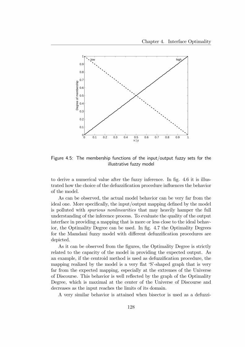
Chapter 4. Interface Optimality
0 0.1 0.2 0.3 0.4 0.5 0.6 0.7 0.8 0.9 10
0.1
0.2
0.3
0.4
0.5
0.6
0.7
0.8
0.9
1
x | y
Deg
ree
of m
embe
rshi
p
low high
Figure 4.5: The membership functions of the input/output fuzzy sets for theillustrative fuzzy model
to derive a numerical value after the fuzzy inference. In fig. 4.6 it is illus-trated how the choice of the defuzzification procedure influences the behaviorof the model.As can be observed, the actual model behavior can be very far from the
ideal one. More specifically, the input/output mapping defined by the modelis polluted with spurious nonlinearities that may heavily hamper the fullunderstanding of the inference process. To evaluate the quality of the outputinterface in providing a mapping that is more or less close to the ideal behav-ior, the Optimality Degree can be used. In fig. 4.7 the Optimality Degreesfor the Mamdani fuzzy model with different defuzzification procedures aredepicted.As it can be observed from the figures, the Optimality Degree is strictly
related to the capacity of the model in providing the expected output. Asan example, if the centroid method is used as defuzzification procedure, themapping realized by the model is a very flat ‘S’-shaped graph that is veryfar from the expected mapping, especially at the extremes of the Universeof Discourse. This behavior is well reflected by the graph of the OptimalityDegree, which is maximal at the center of the Universe of Discourse anddecreases as the input reaches the limits of its domain.A very similar behavior is attained when bisector is used as a defuzzi-
128

4.4. A measure of optimality for Output Interfaces
0 10
1
x
y
Centroid
0 10
1
x
y
Bisector
0 10
1
x
y
Mean of Maxima
0 10
1Lowest of Maxima
x
y
Figure 4.6: The behavior of the fuzzy model according to different choices ofdefuzzification methods
fication procedure. However, the slope of the graph appears a little closerto the ideal mapping. This slight improvement is captured by the GlobalOptimality Degree, which is slightly higher for bisector than for centroid.
A completely symmetrical behavior is shown when mean of maxima isused as a defuzzification procedure. In this case, the model mapping is closerto the ideal behavior at the extremes of the Universe of Discourse, whileit deteriorates at it center. However, on the overall the Global OptimalityDegree shows a better behavior w.r.t. centroid but worse than bisector.
If the lowest of maxima is used as a defuzzification method, an asymmet-rical behavior is observed. In the leftmost side of the Universe of Discourse,the mapping carried out by the model is adherent to the ideal behavior,while on the rightmost side the mapping is unacceptably constant with value1. This behavior is also captured by the trend of the optimality degree. Thebehavior of the model with supremum of maxima defuzzification method isnot shown because it is symmetrical to that emerging from the adoption oflowest of maxima.
129
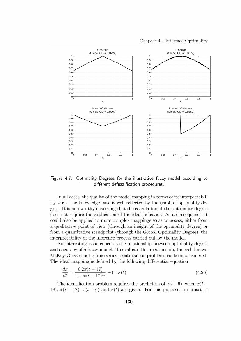
Chapter 4. Interface Optimality
0 10
0.1
0.2
0.3
0.4
0.5
0.6
0.7
0.8
0.9
1
Centroid(Global OD = 0.8222)
x0 0.2 0.4 0.6 0.8 1
0
0.1
0.2
0.3
0.4
0.5
0.6
0.7
0.8
0.9
1
Bisector(Global OD = 0.8677)
x
0 0.2 0.4 0.6 0.8 10
0.1
0.2
0.3
0.4
0.5
0.6
0.7
0.8
0.9
1
Mean of Maxima(Global OD = 0.8397)
x0 0.2 0.4 0.6 0.8 1
0
0.1
0.2
0.3
0.4
0.5
0.6
0.7
0.8
0.9
1
Lowest of Maxima(Global OD = 0.8553)
x
Figure 4.7: Optimality Degrees for the illustrative fuzzy model according todifferent defuzzification procedures.
In all cases, the quality of the model mapping in terms of its interpretabil-ity w.r.t. the knowledge base is well reflected by the graph of optimality de-gree. It is noteworthy observing that the calculation of the optimality degreedoes not require the explication of the ideal behavior. As a consequence, itcould also be applied to more complex mappings so as to assess, either froma qualitative point of view (through an insight of the optimality degree) orfrom a quantitative standpoint (through the Global Optimality Degree), theinterpretability of the inference process carried out by the model.An interesting issue concerns the relationship between optimality degree
and accuracy of a fuzzy model. To evaluate this relationship, the well-knownMcKey-Glass chaotic time series identification problem has been considered.The ideal mapping is defined by the following differential equation
dx
dt=
0.2x(t− 17)1 + x(t− 17)10 − 0.1x(t) (4.26)
The identification problem requires the prediction of x(t+6), when x(t−18), x(t − 12), x(t − 6) and x(t) are given. For this purpose, a dataset of
130
4.5. Final remarks
Table 4.2: Comparison of Optimality Degree and Mean Squared Error for afuzzy model predicting the McKey Glass time series with different defuzzification
methodsDefuzzification Optimality Mean Squared
Method Degree ErrorCentroid 0.4823 0.0212Bisector 0.4608 0.0232
MOM/LOM/SOM 0.3832 0.0647
1000 samples has been generated for t = 118...1117, with the initial conditionx(0) = 1.2. The data have been granulated through the application of theCrisp Double Clustering technique, described in Chapter 8. Based on theresulting information granules, a Mamdani fuzzy model has been designed,which consists of three rules with three inputs and one output.As before, different defuzzification methods are considered for such sys-
tem. For each defuzzification procedure, the Global Optimality Degree andthe Mean Squared Error have been registered as reported in table 4.2. Asit can be seen, the higher is the global optimality degree, the more accurateresults the fuzzy model. This confirms that the optimality degree can be alsoregarded as a quality index of the model under consideration.
4.5 Final remarks
In this Chapter, the issue of interface optimality has been addressed. After aformal specification of Input and Output Interfaces, the optimality conditionhas been analyzed for both types of interfaces. For Input Interfaces, optimal-ity condition can be easily guaranteed if a proper choice of reference fuzzyset is made. In particular, if such fuzzy sets belong to the class of strictly bi-monotonic fuzzy sets (like Gaussian fuzzy sets), optimality condition is easyto guarantee, even if the fuzzy interface is designed by means of data drivenmethods. On the other hand, Input Interfaces based on loosely bi-monotonicfuzzy sets (e.g. triangular shaped) must be designed carefully if optimalitycondition must be met.Differently to Input Interfaces, optimality is hardly satisfied in Output
Interfaces, due to the defuzzification methods that implement them. To stilldeal with the so-called “Information Equivalence Criterion” in Output Inter-faces, a measure of optimality for fuzzy interfaces has been proposed. Themeasure, called Optimality Degree, is defined under a particular condition,i.e. reverse optimality of the Output Interface. The pointwise definition of
131

Chapter 4. Interface Optimality
the optimality degree highlights the variation of quality of the defuzzifica-tion method implementing the Output Interface. The global definition of theoptimality degree provides a quantitative estimate of the quality of the FIS,which may be affected by different design choices.Experimental results have shown that defuzzification methods can be
compared in terms of optimality degrees and a high value of such measure isa necessary condition for accurate fuzzy models. As a design tool, the opti-mality degree can be used to compare different output interfaces (or differentdefuzzification methods), especially when interpretability if of major concernin the design of the model. Furthermore, Optimality Degree could be usedas an objective function that would suggest the investigation of new imple-mentations of Output Interfaces that are specifically aimed at optimizingit.
132

Part III
Algorithms for DerivingInterpretable FuzzyInformation Granules
133

Chapter 5
Gaussian InformationGranulation
5.1 Introduction
The term “Information Granulation” refers to any task aimed at automati-cally generating information granules on the basis of a set of observed exam-ples. When the information granules are semantically represented as multidi-mensional fuzzy sets, the task is called “fuzzy information granulation” andthe generated granules “fuzzy information granules”1. As already mentionedin the first Chapter, the granulation process is fundamental to any intelligentsystem with adaptive behavior.Within the context of interpretable fuzzy modelling, it is necessary that
the information granulation process yields information granules that satisfya set of interpretability requirements. As already observed in the previouschapters, the required interpretability constraints depends on the applicativecontext, on the desired formal representation of granules and, ultimately, onsubjective judgements.In many applicative contexts, especially in control and system identifica-
tion, it is highly desirable that information granules provide a vague repre-sentation of quantities (e.g. “About 10”, “More or Less 2”, “Nearly0”, etc.), as well as spacial information (e.g. cities, lands, etc.). To ad-mit this kind of representation, information granules must satisfy a set ofinterpretability constraints, which include:
• Normality;1Hereafter, as only fuzzy information granulation tasks are analyzed, the adjective
“fuzzy” may be dropped for ease of reading.
135

Chapter 5. Gaussian Information Granulation
• Convexity;• Continuity;In some cases, the Unimodality constraint may be required if vague quan-
tities represent fuzzy numbers or fuzzy points, while this constraint may bedropped when fuzzy intervals or fuzzy regions are allowed. Other inter-pretability constraints may be included according to applicative needs anddesigner judgements, but the three aforementioned constraints constitute theminimal set that is necessary for a proper representation of vague quantities.The automatic generation of fuzzy information granules can be carried
out by means of fuzzy clustering of numerical observations. Fuzzy clusteringalgorithms are extremely useful in finding hidden relationships among dataand hence are widely used for unsupervised learning of empirical knowledge.Unfortunately, in the interpretability context, the adoption of fuzzy clus-tering algorithms may yield to severe drawbacks that must be taken intoaccount. Indeed, many fuzzy clustering algorithms return a set of proto-types and a partition matrix that contains the membership values of eachobservation to each cluster (Bezdek, 1981). Such partition does not conveyany direct information about fuzzy memberships on the entire Universe ofDiscourse, since a column of the partition matrix delineates a discontinuousfuzzy set defined only on the available observations.Furthermore, many clustering algorithms may not produce convex fuzzy
sets, thus the association of linguistic labels to the resulting informationgranules is hard unless further processing is carried out. As an additionaldifficulty, the multi-dimensional clusters cannot be directly projected ontoeach dimension without information loss. This drawback further reduces theutility of fuzzy clustering algorithms in interpretable fuzzy modelling. Finallythe partition matrix is a structure that may need large memory requirements,since its space complexity is linear in the number of observations and inthe number of clusters. This clashes with the simplified representation ofknowledge with highly meaningful linguistic terms.A common approach for the definition of interpretable fuzzy informa-
tion granules is to define them by interpretable fuzzy sets whose parametersare determined by the information provided by the results of a clusteringprocess. In a simplified setting, however, only the derived prototypes areconsidered for determining such parameters, while the information providedby the partition matrix is partially or totally ignored. As an example, ifinterpretable information granules are represented by Gaussian fuzzy sets,the centers of the Gaussian functions are usually made to coincide with theprototypes calculated by the clustering algorithm, while usually no analyt-ical process is adopted to define their widths. Often, heuristic techniques
136
5.1. Introduction
are applied to define the Gaussian widths (Haykin, 1999), but most of themrequire the introduction of some user-defined parameters and do not exploitall the information about the fuzzy clusters discovered by the clustering al-gorithm. Also, the widths are frequently chosen by trial-and-error, and strictassumptions are formulated to simplify the search (e.g. isotropic membershipfunctions with equal widths in all dimensions). The consequence is a largewaste of time that sums up with unexploited useful information provided bythe clustering process.
In this Chapter, a method to induce fuzzy information granules from dataand to represent them by Gaussian functional forms is proposed. First, in-formation granules are extracted from data by a fuzzy clustering algorithm.Then, they are properly represented by Gaussian functions whose widthsare determined by solving a constrained quadratic programming problem onmembership values returned by the clustering algorithm. The method allowscomputation of the widths of Gaussian functions by exploiting the infor-mation conveyed by the partition matrix of the clustering algorithm. Thekey advantage of the proposed approach is the ability to automatically findGaussian representations of fuzzy granules which approximate the member-ship values in the partition matrix with a small Mean Squared Error. Inthe proposed approach, any fuzzy clustering algorithm that returns a set ofprototypes and the corresponding partition matrix can be adopted. Also, theapproach does not require trial-and-error procedures or strong constraints,such as imposing the same width for all the granules (i.e. isotropic Gaussianfunctions).
In the next Section, the proposed method for representation of infor-mation granules induced by fuzzy clustering is introduced. In particular, aGaussian representation is derived by solving a constrained quadratic pro-gramming problem. Then, a rule-based fuzzy model for descriptive modelingis described, as an inference framework in which the derived fuzzy informa-tion granules can be applied. Finally, a real-world information granulationproblem is considered to validate the proposed method. Also, the sectionincludes the development of a descriptive fuzzy model for MPG (miles perGallon) prediction benchmark. The Chapter ends with some conclusive re-marks.
137
Chapter 5. Gaussian Information Granulation
5.2 Amethod of Information Granulation withGaussian fuzzy sets
Gaussian fuzzy sets are especially useful in representing interpretable infor-mation granules. Indeed, they satisfy several interpretability requirements— included those considered in this study — and have the added value of adifferentiable functional form that is valuable in many adaptive models. Aninteresting issue concerns the generation of fuzzy information granules se-mantically represented by Gaussian fuzzy sets by exploiting the results ofa clustering process. In this Section, this issue is pursued and an efficientmethod is proposed.On a formal level, a fuzzy clustering algorithm can be described as a
function that accepts a set of observations and returns a set of prototypestogether with a partition matrix. The number of clusters (i.e. informationgranules) may be predefined or determined by the algorithm. Hence, a genericfuzzy clustering algorithm may be formalized as:
fc : UN → Uc × [0, 1]m×c (5.1)
for U ⊆ Rn, N > 1, c ≥ 1 and such that:
fc (x1,x2, . . . ,xN) = hP,Mi (5.2)
where:
P = [p1,p2, . . . ,pc] (5.3)
is the matrix of all prototypes (one for each column), and:
M = [m1,m2, . . . ,mc] = [mij]i=1,2,...,Nj=1,2,...,c
(5.4)
is the partition matrix, that contains the membership value of each observa-tion to each cluster.
5.2.1 Problem formulation
Given the result of a fuzzy clustering algorithm, the objective of the proposedmethod is to find a set of Gaussian representations of the discovered clusters,corresponding to the following functional form:
µ[ω,C] (x) = exp³− (x− ω)C−1 (x− ω)T
´(5.5)
138

5.2. A method of Information Granulation with Gaussian fuzzy sets
where ω is the center and C−1 is the inverse of the width matrix. Ma-trix C−1 should be symmetric positive definite (s.p.d.) in order to have aconvex shape centered on ω of the function graph. Nevertheless, to achieveinterpretability of the resulting granule, the membership function should beprojected onto each axis without any loss of information. This can be at-tained if the amplitude matrix has non-zero elements only in its principaldiagonal. Indeed, if C−1 is a diagonal matrix, that is:
C−1 = diag c = diag (c1, c2, . . . , cn) , ci > 0 (5.6)
then the fuzzy granule can be represented as product of independent scalarexponential functions2:
µ[ω,C] (x) =nYi=1
µ[ωi,ci] (xi) =nYi=1
exp¡−ci (xi − ωi)
2¢ (5.7)
where the product can be conveniently interpreted as the conjunction oper-ation of fuzzy sets.The problem of finding membership parameters can be decomposed into
c independent sub-problems that find the best representation for each clusterdiscovered by the clustering algorithm. Hence, in the following the analysisis focused on a single cluster and the cluster index j is dropped — whenunnecessary — for ease of reading.Generally, there is no an exact solution to the problem, i.e. there is not
a pair hω,Ci such that:∀i : µ[ω,C] (xi) = mi (5.8)
with the constraint:
∀x 6= 0 : xTC−1x > 0 (5.9)
In order to choose the “best” Gaussian representation, some error functionhas to be defined. Because of the nonlinearity of the equations in (5.8), it isnot possible to apply general linear systems theory. On the other hand, theequation system in (5.8) is equivalent to the following:
∀i : − (xi − ω)T C−1 (xi − ω) = logmi, C−1s.p.d. (5.10)
The system (5.10) can be rewritten as:
∀i : bxiTC−1 bxi = − logmi, C−1s.p.d. (5.11)
2Each unidimensional Gaussian fuzzy set can be reconducted to the canonical formwith the definition σi = 1/2ci
139

Chapter 5. Gaussian Information Granulation
where the center of the Gaussian membership function is put equal to thecluster prototype:
ω = pj (5.12)
and the following change of variables is done:
bxi = xi − ω (5.13)
By imposing C to be positive diagonal, the system can be further simplifiedas:
∀i :nX
k=1
cxik2ck = − logmi, ci > 0 (5.14)
where
bxi = [cxik]k=1,2,...,n (5.15)
The equations in (5.14) form a constrained linear system; generally, ithas not an exact solution, so a constrained least squared error minimizationproblem can be formulated as follows:
minimize: f (c) = 1N
PNi=1
¡Pnk=1 cxik2ck + logmi
¢2subject to: c > 0
(5.16)
To solve the minimization problem (5.16) the following matrix is defined:
H =£cxik2¤i=1,2,...,N
k=1,2,...,n(5.17)
then, excluding the constant terms, the problem (5.16) can be restated as:
minimize: f 0 (c) = 12cTGc+ gTc
subject to: c > 0(5.18)
where:
G = 2HTH (5.19)
and:
g = 2HT logm (5.20)
140
5.2. A method of Information Granulation with Gaussian fuzzy sets
The problem (5.18) can be solved with classical constrained quadraticprogramming techniques. Usually, quadratic programming algorithms onlyaccept constraints in the form:
Ac ≥ b (5.21)
In this case, it is useful to express the constraints of the objective functionin the form:
c ≥ cmin (5.22)
where the vector cmin defines the maximum admissible amplitudes. Ifcmin = 0, then all possible amplitudes are admissible, even infinite.
5.2.2 Analysis of the solution
In order to analyze the optimal solution of (5.18) with respect to the originalproblem setting (5.8), it is useful to rewrite the objective function f as:
f (c) =1
N
NXi=1
log exp³−bxiT · diag c · bxi´
mi
2
(5.23)
which is the mean squared log-ratio between the Gaussian membership ap-proximation and the actual membership value assigned by the clusteringalgorithm. The squared log-ratio is a concave positive function with globalminimum in 1 with value 0 (see fig. 5.1).By expanding the Taylor series of the squared log-ratio with center in 1,
it is possible to observe that in a sufficiently small neighbor of point 1, thefunction is equal to:
(log ξ)2 = (ξ − 1)2 +O¡(ξ − 1)3¢ (5.24)
In such neighborhood, the following approximation can be done:
ε =
µlog
µ[ω,C] (xi)
mi
¶2≈µµ[ω,C] (xi)
mi− 1¶2
(5.25)
This implies that:¡µ[ω,C] (xi)−mi
¢2 ≈ m2i ε ≤ ε (5.26)
As a consequence, if the log-ratio assumes small values, the resultingGaussian membership function approximates the partition matrix with asmall Mean Squared Error. This property validates the proposed approach.
141
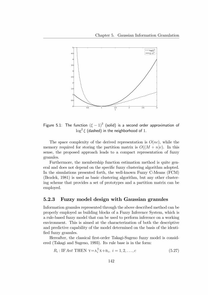
Chapter 5. Gaussian Information Granulation
0.5 1 1.5 2 2.5 30
0.5
1
1.5
2
2.5
3
3.5
4
4.5
5
ξ
log(ξ)2
(ξ−1)2
Figure 5.1: The function (ξ − 1)2 (solid) is a second order approximation oflog2 ξ (dashed) in the neighborhood of 1.
The space complexity of the derived representation is O(nc), while thememory required for storing the partition matrix is O((M + n)c). In thissense, the proposed approach leads to a compact representation of fuzzygranules.Furthermore, the membership function estimation method is quite gen-
eral and does not depend on the specific fuzzy clustering algorithm adopted.In the simulations presented forth, the well-known Fuzzy C-Means (FCM)(Bezdek, 1981) is used as basic clustering algorithm, but any other cluster-ing scheme that provides a set of prototypes and a partition matrix can beemployed.
5.2.3 Fuzzy model design with Gaussian granules
Information granules represented through the above described method can beproperly employed as building blocks of a Fuzzy Inference System, which isa rule-based fuzzy model that can be used to perform inference on a workingenvironment. This is aimed at the characterization of both the descriptiveand predictive capability of the model determined on the basis of the identi-fied fuzzy granules.Hereafter, the classical first-order Takagi-Sugeno fuzzy model is consid-
ered (Takagi and Sugeno, 1993). Its rule base is in the form:
Ri : IFAnt THEN y=aTi x+bi, i = 1, 2, . . . , c (5.27)
142
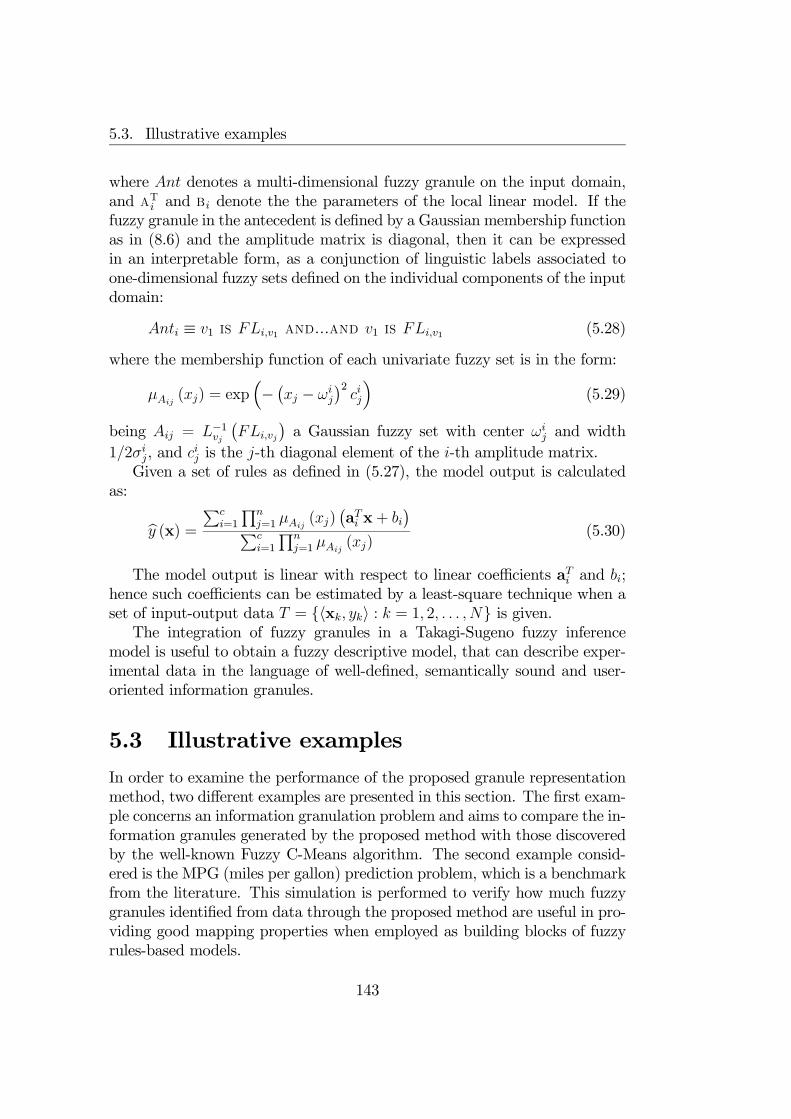
5.3. Illustrative examples
where Ant denotes a multi-dimensional fuzzy granule on the input domain,and aTi and bi denote the the parameters of the local linear model. If thefuzzy granule in the antecedent is defined by a Gaussian membership functionas in (8.6) and the amplitude matrix is diagonal, then it can be expressedin an interpretable form, as a conjunction of linguistic labels associated toone-dimensional fuzzy sets defined on the individual components of the inputdomain:
Anti ≡ v1 is FLi,v1 and...and v1 is FLi,v1 (5.28)
where the membership function of each univariate fuzzy set is in the form:
µAij(xj) = exp
³− ¡xj − ωi
j
¢2cij
´(5.29)
being Aij = L−1vj¡FLi,vj
¢a Gaussian fuzzy set with center ωi
j and width1/2σij, and cij is the j-th diagonal element of the i-th amplitude matrix.Given a set of rules as defined in (5.27), the model output is calculated
as:
by (x) = Pci=1
Qnj=1 µAij
(xj)¡aTi x+ bi
¢Pci=1
Qnj=1 µAij
(xj)(5.30)
The model output is linear with respect to linear coefficients aTi and bi;hence such coefficients can be estimated by a least-square technique when aset of input-output data T = hxk, yki : k = 1, 2, . . . , N is given.The integration of fuzzy granules in a Takagi-Sugeno fuzzy inference
model is useful to obtain a fuzzy descriptive model, that can describe exper-imental data in the language of well-defined, semantically sound and user-oriented information granules.
5.3 Illustrative examples
In order to examine the performance of the proposed granule representationmethod, two different examples are presented in this section. The first exam-ple concerns an information granulation problem and aims to compare the in-formation granules generated by the proposed method with those discoveredby the well-known Fuzzy C-Means algorithm. The second example consid-ered is the MPG (miles per gallon) prediction problem, which is a benchmarkfrom the literature. This simulation is performed to verify how much fuzzygranules identified from data through the proposed method are useful in pro-viding good mapping properties when employed as building blocks of fuzzyrules-based models.
143

Chapter 5. Gaussian Information Granulation
Figure 5.2: The North-East Dataset
5.3.1 Information granulation of postal addresses
As an information granulation problem, the North East dataset is chosen,containing 123,593 postal addresses (represented as normalized coordinates,see fig. 5.2), which represent the three metropolitan areas of New York,Philadelphia and Boston. (Kollios et al., 2003). The dataset can be groupedinto three clusters, with a lot of noise, in the form of uniformly distributedrural areas and smaller population centers.The FCM algorithm has been used to generate three fuzzy clusters from
the dataset. Successively, the prototype vector and the partition matrixreturned by FCM were used by the proposed method to obtain a Gaussianrepresentation of the three clusters. For FCM and quadratic programming,the Matlab R° R11.1 Fuzzy toolbox and Optimization toolbox have been usedrespectively.Centers and widths of the derived Gaussian functions are reported in
table 5.1. Figures 5.3, 5.4 and 5.5, depict for each cluster both membershipvalues in the partition matrix as grey-levels, and the radial contours of thecorresponding Gaussian function.As it can be seen in the figures, Gaussian granules obtained by the pro-
posed approach properly model some qualitative concepts about the available
144

5.3. Illustrative examples
Table 5.1: Parameters of the Gaussian Information Granules and Mean SquaredError
Boston New York PhiladelphiaCenter (0.6027, 0.6782) (0.3858, 0.4870) (0.1729, 0.2604)Amplitudes (0.0906, 0.1027) (0.0580, 0.0606) (0.1013, 0.1151)MSE 0.0360 0.0203 0.0347
Figure 5.3: Fuzzy granule for Philadelphia city and its Gaussian representation
145
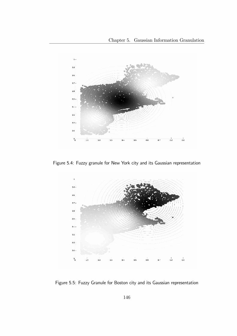
Chapter 5. Gaussian Information Granulation
Figure 5.4: Fuzzy granule for New York city and its Gaussian representation
Figure 5.5: Fuzzy Granule for Boston city and its Gaussian representation
146
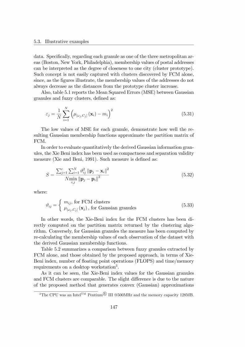
5.3. Illustrative examples
data. Specifically, regarding each granule as one of the three metropolitan ar-eas (Boston, New York, Philadelphia), membership values of postal addressescan be interpreted as the degree of closeness to one city (cluster prototype).Such concept is not easily captured with clusters discovered by FCM alone,since, as the figures illustrate, the membership values of the addresses do notalways decrease as the distances from the prototype cluster increase.Also, table 5.1 reports the Mean Squared Errors (MSE) between Gaussian
granules and fuzzy clusters, defined as:
εj =1
N
NXi=1
³µ[ωj ,Cj ] (xi)−mi
´2(5.31)
The low values of MSE for each granule, demonstrate how well the re-sulting Gaussian membership functions approximate the partition matrix ofFCM.In order to evaluate quantitatively the derived Gaussian information gran-
ules, the Xie Beni index has been used as compactness and separation validitymeasure (Xie and Beni, 1991). Such measure is defined as:
S =
Pcj=1
PNi=1 ϑ
2ij kpj − xik2
Nmini,jkpj − pik2
(5.32)
where:
ϑij =
½mij, for FCM clustersµ[ωj ,Cj ] (xj) , for Gaussian granules
(5.33)
In other words, the Xie-Beni index for the FCM clusters has been di-rectly computed on the partition matrix returned by the clustering algo-rithm. Conversely, for Gaussian granules the measure has been computed byre-calculating the membership values of each observation of the dataset withthe derived Gaussian membership functions.Table 5.2 summarizes a comparison between fuzzy granules extracted by
FCM alone, and those obtained by the proposed approach, in terms of Xie-Beni index, number of floating point operations (FLOPS) and time/memoryrequirements on a desktop workstation3.As it can be seen, the Xie-Beni index values for the Gaussian granules
and FCM clusters are comparable. The slight difference is due to the natureof the proposed method that generates convex (Gaussian) approximations
3The CPU was an IntelTM Pentium R° III @500MHz and the memory capacity 128MB.
147
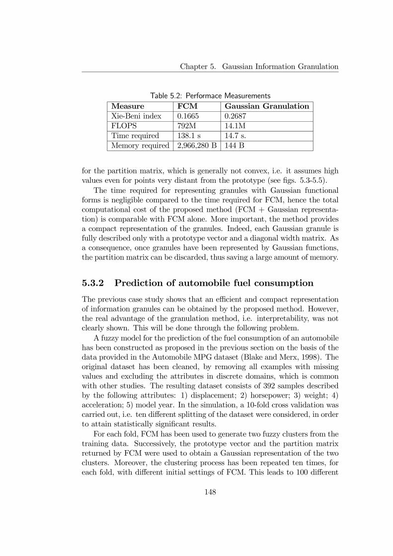
Chapter 5. Gaussian Information Granulation
Table 5.2: Performace MeasurementsMeasure FCM Gaussian GranulationXie-Beni index 0.1665 0.2687FLOPS 792M 14.1MTime required 138.1 s 14.7 s.Memory required 2,966,280 B 144 B
for the partition matrix, which is generally not convex, i.e. it assumes highvalues even for points very distant from the prototype (see figs. 5.3-5.5).The time required for representing granules with Gaussian functional
forms is negligible compared to the time required for FCM, hence the totalcomputational cost of the proposed method (FCM + Gaussian representa-tion) is comparable with FCM alone. More important, the method providesa compact representation of the granules. Indeed, each Gaussian granule isfully described only with a prototype vector and a diagonal width matrix. Asa consequence, once granules have been represented by Gaussian functions,the partition matrix can be discarded, thus saving a large amount of memory.
5.3.2 Prediction of automobile fuel consumption
The previous case study shows that an efficient and compact representationof information granules can be obtained by the proposed method. However,the real advantage of the granulation method, i.e. interpretability, was notclearly shown. This will be done through the following problem.A fuzzy model for the prediction of the fuel consumption of an automobile
has been constructed as proposed in the previous section on the basis of thedata provided in the Automobile MPG dataset (Blake and Merx, 1998). Theoriginal dataset has been cleaned, by removing all examples with missingvalues and excluding the attributes in discrete domains, which is commonwith other studies. The resulting dataset consists of 392 samples describedby the following attributes: 1) displacement; 2) horsepower; 3) weight; 4)acceleration; 5) model year. In the simulation, a 10-fold cross validation wascarried out, i.e. ten different splitting of the dataset were considered, in orderto attain statistically significant results.For each fold, FCM has been used to generate two fuzzy clusters from the
training data. Successively, the prototype vector and the partition matrixreturned by FCM were used to obtain a Gaussian representation of the twoclusters. Moreover, the clustering process has been repeated ten times, foreach fold, with different initial settings of FCM. This leads to 100 different
148

5.3. Illustrative examples
Table 5.3: Average RMSE of the 10 Takagi-Sugeno models identified from eachfold. The total mean of RMSE is reported in the last row
Average Error on Average Error onFold Training set Test set1 3.05 2.552 2.58 3.063 2.81 2.824 2.86 2.835 2.71 2.926 2.71 3.017 2.67 2.968 2.66 2.949 2.90 2.7510 2.88 2.74Mean 2.78 2.86
granulations of the data in total.Then, using the information granules resulting from each granulation
process, a Takagi-Sugeno model with two rules has been built as previouslydescribed. The prediction ability of the identified fuzzy models has beenevaluated both on the training set and the test set in terms of root meansquared error (RMSE):
RMSE(T ) =
s1
|T |X
hx,yi∈T
(y − by (x))2 (5.34)
Results of such experiments are summarized in table 5.3 which reports, foreach fold, the average RMSE of the 10 TS models identified. Also, the totalmean of RMSE is reported, as an estimate of the prediction capability of thefuzzy inference model based on information granules derived by the proposedapproach. This value shows a good predictive accuracy for such a fuzzy modelas compared with previously reported results. Indeed, very similar resultsare reported by Abonyi, Babuška and Szeifert (Abonyi et al., 2002), wherea modified version of Gath-Geva clustering that extracts Gaussian clusterswith diagonal amplitude matrices is proposed. With a two-rule model, sucha method achieved RMSE value of 2.72 and 2.85 for training and test data.However, it should be noted that these results derive from a single partitionof the dataset, and hence they are not statistically significant.For a further comparison, fuzzy models with only two input variables,
namely the Weight and the Year, as suggested by Jang (Jang, 1996), were
149
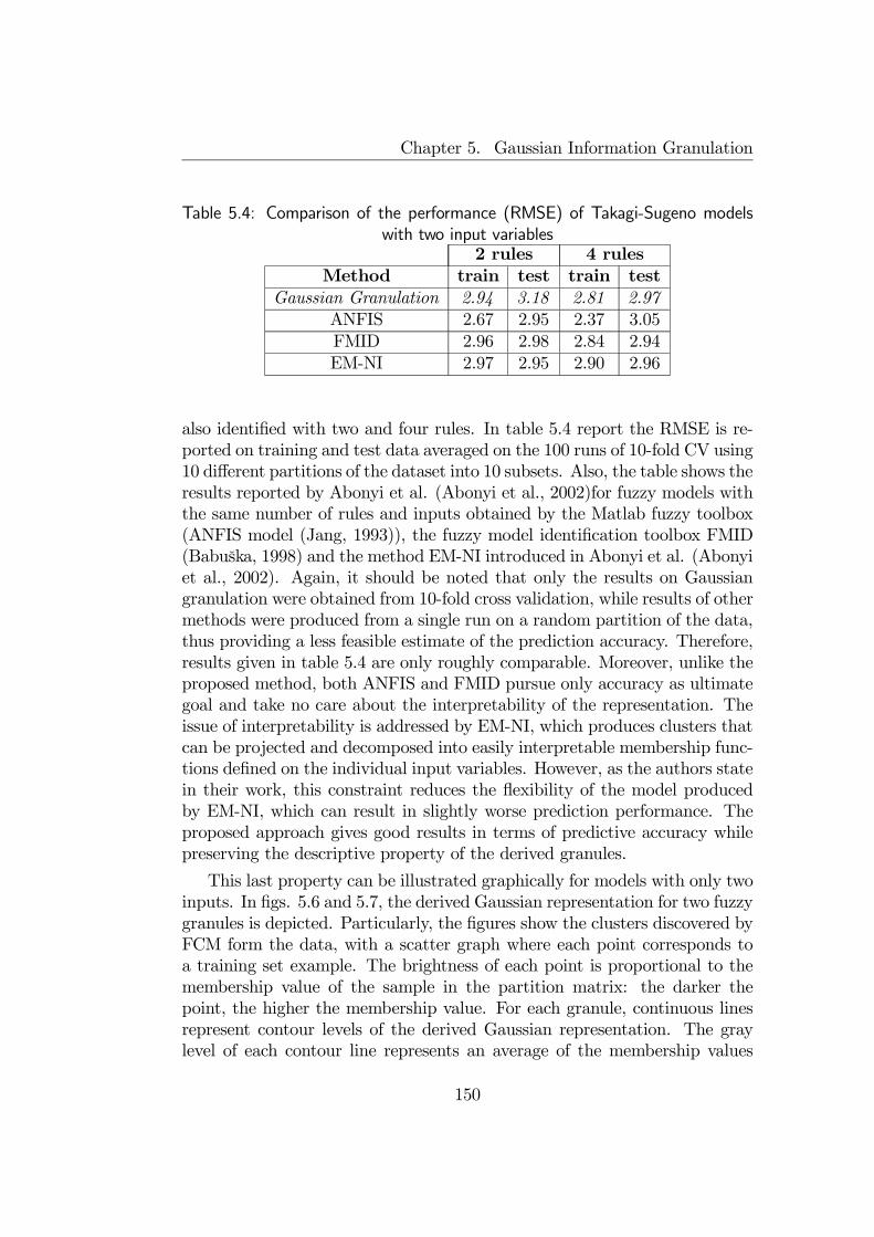
Chapter 5. Gaussian Information Granulation
Table 5.4: Comparison of the performance (RMSE) of Takagi-Sugeno modelswith two input variables
2 rules 4 rulesMethod train test train test
Gaussian Granulation 2.94 3.18 2.81 2.97ANFIS 2.67 2.95 2.37 3.05FMID 2.96 2.98 2.84 2.94EM-NI 2.97 2.95 2.90 2.96
also identified with two and four rules. In table 5.4 report the RMSE is re-ported on training and test data averaged on the 100 runs of 10-fold CV using10 different partitions of the dataset into 10 subsets. Also, the table shows theresults reported by Abonyi et al. (Abonyi et al., 2002)for fuzzy models withthe same number of rules and inputs obtained by the Matlab fuzzy toolbox(ANFIS model (Jang, 1993)), the fuzzy model identification toolbox FMID(Babuška, 1998) and the method EM-NI introduced in Abonyi et al. (Abonyiet al., 2002). Again, it should be noted that only the results on Gaussiangranulation were obtained from 10-fold cross validation, while results of othermethods were produced from a single run on a random partition of the data,thus providing a less feasible estimate of the prediction accuracy. Therefore,results given in table 5.4 are only roughly comparable. Moreover, unlike theproposed method, both ANFIS and FMID pursue only accuracy as ultimategoal and take no care about the interpretability of the representation. Theissue of interpretability is addressed by EM-NI, which produces clusters thatcan be projected and decomposed into easily interpretable membership func-tions defined on the individual input variables. However, as the authors statein their work, this constraint reduces the flexibility of the model producedby EM-NI, which can result in slightly worse prediction performance. Theproposed approach gives good results in terms of predictive accuracy whilepreserving the descriptive property of the derived granules.
This last property can be illustrated graphically for models with only twoinputs. In figs. 5.6 and 5.7, the derived Gaussian representation for two fuzzygranules is depicted. Particularly, the figures show the clusters discovered byFCM form the data, with a scatter graph where each point corresponds toa training set example. The brightness of each point is proportional to themembership value of the sample in the partition matrix: the darker thepoint, the higher the membership value. For each granule, continuous linesrepresent contour levels of the derived Gaussian representation. The graylevel of each contour line represents an average of the membership values
150

5.3. Illustrative examples
Figure 5.6: First granule representation
relative to the points laying in the contours neighbors.These fuzzy information granules can be easily projected onto each axis,
yielding interpretable Frames of Cognition defined on each input feature,as depicted in figs. 5.8 and 5.9. As it can be seen, for each variable, thetwo fuzzy sets are represented by very distinct membership functions thatturn out to be nicely interpretable. As a consequence, each one-dimensionalfuzzy set can be easily associated to a quantitative linguistic label, such as“About 2500 Kg”, “About 3500 Kg”, “About 1973”, “About 1979”.Such linguistic labels can be used in the formulation of fuzzy rules, as thefollowings:
R1: IF weight is About 2500 Kg AND year is About1973 THEN mpg = f1(weight, year)
R2: IF weight is About 3500 Kg AND year is About1979 THEN mpg = f2(weight, year)
where:
f1 (w, y) =−4.1241000
w +27.24
100y + 12.62 (5.35a)
f2 (w, y) =−10.531000
w +60.68
100y + 9.069 (5.35b)
151

Chapter 5. Gaussian Information Granulation
Figure 5.7: Second granule representation
Figure 5.8: The Frame of Cognition for the “Weight” variable
152
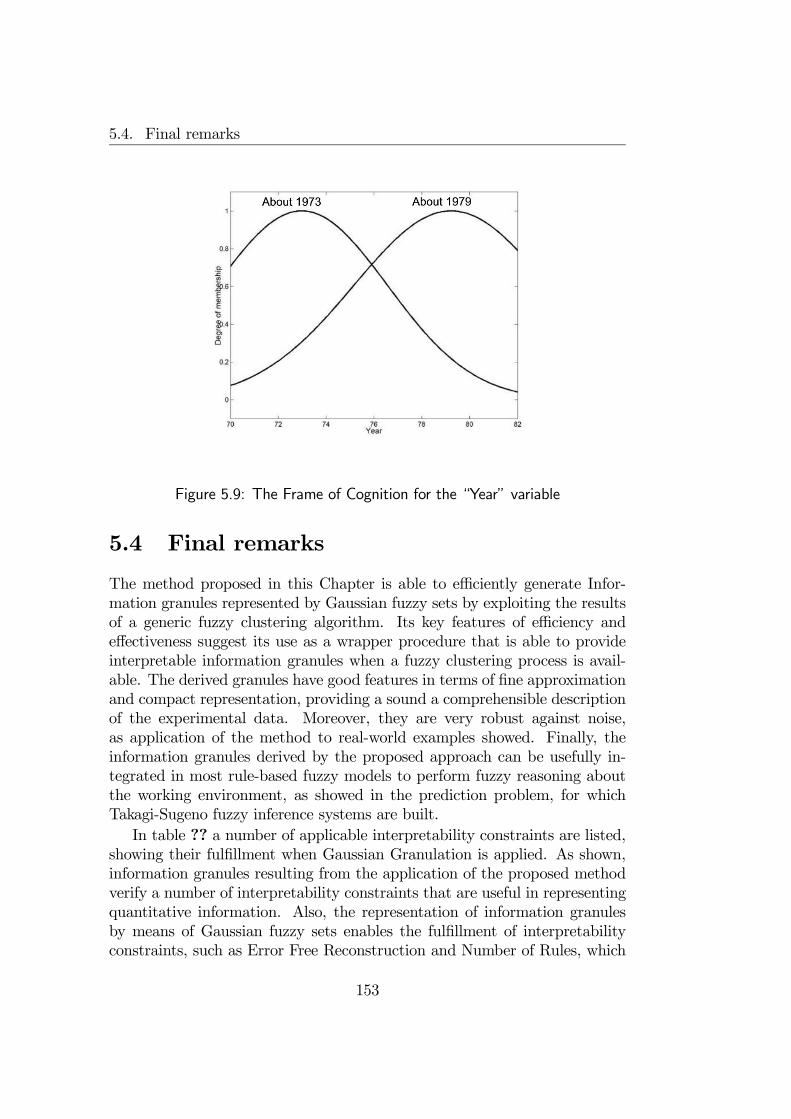
5.4. Final remarks
Figure 5.9: The Frame of Cognition for the “Year” variable
5.4 Final remarks
The method proposed in this Chapter is able to efficiently generate Infor-mation granules represented by Gaussian fuzzy sets by exploiting the resultsof a generic fuzzy clustering algorithm. Its key features of efficiency andeffectiveness suggest its use as a wrapper procedure that is able to provideinterpretable information granules when a fuzzy clustering process is avail-able. The derived granules have good features in terms of fine approximationand compact representation, providing a sound a comprehensible descriptionof the experimental data. Moreover, they are very robust against noise,as application of the method to real-world examples showed. Finally, theinformation granules derived by the proposed approach can be usefully in-tegrated in most rule-based fuzzy models to perform fuzzy reasoning aboutthe working environment, as showed in the prediction problem, for whichTakagi-Sugeno fuzzy inference systems are built.In table ?? a number of applicable interpretability constraints are listed,
showing their fulfillment when Gaussian Granulation is applied. As shown,information granules resulting from the application of the proposed methodverify a number of interpretability constraints that are useful in representingquantitative information. Also, the representation of information granulesby means of Gaussian fuzzy sets enables the fulfillment of interpretabilityconstraints, such as Error Free Reconstruction and Number of Rules, which
153
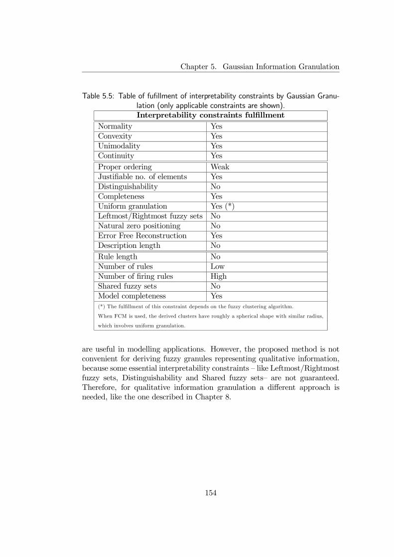
Chapter 5. Gaussian Information Granulation
Table 5.5: Table of fufillment of interpretability constraints by Gaussian Granu-lation (only applicable constraints are shown).Interpretability constraints fulfillment
Normality YesConvexity YesUnimodality YesContinuity YesProper ordering WeakJustifiable no. of elements YesDistinguishability NoCompleteness YesUniform granulation Yes (*)Leftmost/Rightmost fuzzy sets NoNatural zero positioning NoError Free Reconstruction YesDescription length NoRule length NoNumber of rules LowNumber of firing rules HighShared fuzzy sets NoModel completeness Yes(*) The fulfillment of this constraint depends on the fuzzy clustering algorithm.
When FCM is used, the derived clusters have roughly a spherical shape with similar radius,
which involves uniform granulation.
are useful in modelling applications. However, the proposed method is notconvenient for deriving fuzzy granules representing qualitative information,because some essential interpretability constraints — like Leftmost/Rightmostfuzzy sets, Distinguishability and Shared fuzzy sets— are not guaranteed.Therefore, for qualitative information granulation a different approach isneeded, like the one described in Chapter 8.
154
Chapter 6
Minkowski InformationGranulation
6.1 Introduction
In the previous Chapter, a method has been proposed with the specific aimof generating information granules representing vague numbers or vectors. Inother applicative contexts, however, a different type of granular informationmay be required, as one representing intervals or hyper-boxes1 (either crispor fuzzy). In this case, Gaussian granulation may not be convenient sincethe generated granules represent fuzzy vectors that have an elliptical — ratherthan boxed — distribution of membership degrees (see fig. 6.1).To generate box-shaped fuzzy information granules, a different approach
for information granulation is proposed in this Chapter. The described ap-proach is based on that presented in (Bargiela and Pedrycz, 2003b) andconsists in decomposing complex topologies of data structures through hi-erarchical partitioning of the structures into core and residual parts. Thecores are represented as granular prototypes characterized by a transparentboxlike shape that can be interpreted as a decomposable relation among datafeatures.To generate the granular prototypes, the Minkowski Fuzzy C-Means has
been investigated as a tool that allows a degree of control over the geometryof the information granules identified through clustering. The transition fromhyper-ellipsoids to hyper-boxes, prompted by the change of the order of theMinkowski distance from 2 to ∞, is somewhat distorted by two concurrentfactors subject of study: the Minkowski order and the interactions amongclusters.
1A hyper-box (or hyper-interval) is the Cartesian product of one or more intervals.
155

Chapter 6. Minkowski Information Granulation
(a) (b)
Figure 6.1: Two distributions of membership degrees: (a) elliptical distribution;(b) boxed distribution.
The first deformation factor is due to the estimation error introducedwhen approximating the Tchebychev distance — which characterizes boxlikegranules — with Minkowski distances. To investigate such phenomenon, afirst distortion measure is formalized to quantify the approximation error inrelation to the Minkowski order. Experimental results show that such distor-tion measure quickly decreases as the Minkowski order increases, but calculiwith too high orders are hampered by perturbation errors involved by finiteprecision arithmetic. As a consequence the distortion measure can be usedas a tool to estimate the best Minkowski order that allows the approximationto the Tchebychev on a given machine.
The second deformation effect is due to interactions among clusters, whichdistort the boxlike shape of clusters to meet the constraints required byFuzzy C-Means. To deal with such problem, a second deformation measurehas been formalized. This measure evaluates the distortion of each clusterα-cut with an associated “ideal” hyper-box. With the aid of such measure,boxlike granular prototypes can be generated within an accepted deformationthreshold.
In the next section, the Minkowski Fuzzy C-Means is described in detail.Then, the approach for extracting interpretable information granules is for-malized, and a study on the deformation effects is presented. Finally, someillustrative material is portrayed so as to exemplify the key results of thestudy from a practical viewpoint.
156

6.2. A method for Information Granulation through Minkowski fuzzyclustering
6.2 A method for Information Granulationthrough Minkowski fuzzy clustering
In this Section, the proposed method for information granulation throughMinkowski fuzzy clustering is described. First, the Minkowski Fuzzy C-Means is formalized and its algorithmic issues are analyzed. Then, themethod for information granulation is described with a number of theoreticalconsiderations.
6.2.1 Minkowski Fuzzy C-Means
Let be a set of data patterns to be clustered into fuzzy partitions by mini-mizing the following objective function:
Q =cX
i=1
NXk=1
m2ikd
(p)ik (6.1)
where [mik]k=1,2,...,Ni=1,2,...,c is the partition matrix, which is subject to:
∀k :cX
i=1
mik = 1 (6.2a)
∀i, k : 0 ≤ mik ≤ 1 (6.2b)
∀i : 0 <NXk=1
mik < N (6.2c)
The distance between a pattern xk and a cluster prototype vi is denotedby d(p)ik and is defined as:
d(p)ik =
p
vuut nXj=1
|xkj − vij|p (6.3)
being p the order of the Minkowski distance xk = (xk1, xk2, . . . , xkn), andvi = (vi1, vi2, . . . , vin). The objective of Minkowski Fuzzy C-Means is to finda proper choice of the partition matrix [mik] and prototypes v1,v2, . . . ,vcsuch that (6.1) is minimal while satisfying constraints in (6.2).Such minimization problem has been tackled specifically for Minkowski
distances in (Groenen and Jajuga, 2001). There, the authors propose agradient-free minimization method called “iterative majorization” (Groenenet al., 1995). However, such method cannot be applied for p > 2, it is
157
Chapter 6. Minkowski Information Granulation
not suitable to generate boxlike information granules. As a consequence,an extension of the classical Fuzzy C-Means procedure has been devised tofit Minkowski distance. Fuzzy C-Means is standard to a high extent and isbased on alternative optimization of the partition matrix [mik] and the setof prototypes v1,v2, . . . ,vc (Bezdek, 1981). These two steps are repeatediteratively until no significant change of the objective function is registered.The update formula of the partition matrix does not depend on the chosendistance function and is derived by means of Lagrange multipliers. Aftersome straightforward calculations, the following expression can be obtained:
mst [τ + 1] =1Pc
j=1d(p)st [τ ]
d(p)jt [τ ]
(6.4)
Here, the variable τ denotes the iteration number. Differently from thepartition matrix, the derivation of the update formula for the cluster proto-types depends on the analytical form of the distance function. Specifically,the update formula is determined by solving the following equation system:
∂Q
∂vst= 0,
s = 1, 2, . . . , ct = 1, 2, . . . , n
(6.5)
Such equation system has a simple solution for p = 2 while cannot besolved analytically for a generic order p. For such reason, the update formulafor each prototypes follows the gradient-descent scheme:
vst [τ + 1] = vst [τ ]− α∂Q
∂vst(6.6)
Such scheme introduces a novel hyper-parameter α whose value is criticalfor the convergence of the iterations. However, based on empirical observa-tions, the following choice always leads to convergence:
α ∝ 1
N(6.7)
The derivatives of the objective function with respect to each prototypeare calculated as follows:
∂Q
∂vst=
NXk=1
m2sk
∂
∂vstd(p)sk (6.8)
where:
∂
∂vstd(p)sk = −
³d(p)sk
´1−p· |xkt − vst| · sgn (xkt − vst) (6.9)
158
6.2. A method for Information Granulation through Minkowski fuzzyclustering
being sgn the sign function.Although the case of p = +∞ is not included in such computation, it
should be remarked that the Tchebychev distance can be handled through afuzzy logic approximation of the ‘max’ operation as discussed in (Castellanoet al., 2004). In particular, for pÀ 1 the corresponding Minkowski distancequickly approaches the Tchebychev distance, hence the Minkowski Fuzzy C-Means can be applied to derive box-shaped information granules by using agradient descent scheme.In summary, the clustering algorithm can be described as a sequence of
the following steps:
1. Randomly define prototypes
2. Repeat
(a) Compute the partition matrix according to (4)
(b) Compute prototypes according to (6)
3. Until a termination criterion is satisfied
The most commonly adopted termination criterion entails the variationof the objective function. Specifically, it is met when:
Q [τ + 1]−Q [τ ] < ε (6.10)
being ε a user-defined threshold. Note that while the update formula of thepartition matrix is the same as for the standard Fuzzy C-Means, the updateof the prototypes is more time consuming.
6.2.2 Generation of Information Granules
The Minkowski order p used for clustering is user defined and is chosen so asto achieve a control over the shape of the information granules. It should beremarked that as p→ +∞, the distance function approaches the Tchebychevdistance defined as:
d(∞)ik = max
j=1,2,...,n|xkj − vij| (6.11)
Such distance function is well suited to identify box-shaped informationgranules that can be represented as a decomposable relation R identified asa Cartesian product of one-dimensional information granules:
R = R1 ×R2 × · · · ×Rn (6.12)
159
Chapter 6. Minkowski Information Granulation
Such decomposability leads to transparent information granules and canbe effectively adopted in data mining contexts. On the other hand, for p = 2,the Minkowski Fuzzy C-Means reduces to the classical Fuzzy C-Means basedon Euclidean distance, which is used to extract ellipsoidal-shaped informationgranules that are not decomposable in the aforementioned sense. As a conse-quence, an interesting study concerns the quantification of the deformationeffects of information granules in relation to the Minkowski order.Once the final partition matrix has been computed, c multidimensional
fuzzy sets G1, . . . ,Gc can be defined by the following membership functions:
mi (x) =
(δij, if x = vj for some j³Pc
j=1d(p)(x,vi)
d(p)(x,vj)
´−1, otherwise
(6.13)
being:
d(p) (x,v) = p
vuut nXj=1
|xj − vj|p (6.14)
and δij the Kronecker’s symbol. Definition (6.13) is a direct extension ofequation (6.4) in a functional form.In a small neighborhood of vi, the contour levels of the i-th fuzzy set
have approximately the same shape of the distance function. Indeed, if fori 6= j : d(p) (x,vi)¿ d(p) (x,vj), then:
mi (x) ≈ 1− βd(p) (x,vi) (6.15)
being β a positive constant. As the distance between x and increases vi, theinteractions amongst the different clusters become stronger, and the shapeof the contour levels will distort significantly.By virtue of (6.15), for pÀ 1 the contour levels of the fuzzy sets assume
the shape of a hyper-box in the neighborhood of each prototype. To assessthe distortion involved in approximating the Tchebychev distance with aMinkowski distance, the following measure can be adopted:
∆(p) =cX
i=1
ZU
|mi (x)−mi (x)| (6.16)
being:
mi (x) =
(δij, if x = vj for some j³Pc
j=1d(∞)(x,vi)
d(∞)(x,vj)
´−1, otherwise
(6.17)
160

6.2. A method for Information Granulation through Minkowski fuzzyclustering
The measure ∆(p) is theoretical and cannot be evaluated in any analyticalway. Nevertheless, it can be estimated as:
D(p) =1
N
cXi=1
NXk=1
|mi (xk)−mi (xk)| (6.18)
From a theoretical point of view, it is expected that:
limp→∞
D(p) = 0 (6.19)
However, when the Minkowski Fuzzy C-Means is executed on a digitalcomputer, it is possible that for very high values of p numerical errors sig-nificantly perturb the convergence (6.19). As a consequence, the measure(6.18) can be used to evaluate the maximum value of p that allows the bestapproximation of the Tchebychev distance on a given digital computer.Once the most suitable value p of has been selected, the geometric proper-
ties of the information granules can be studied. As an example, in (Bargielaand Pedrycz, 2003b) an approach is proposed to evaluate the deformation ofmembership grades due to cluster interactions when box-shaped informationgranules are required. To quantify such deformation, the γ-cuts of each fuzzyset are considered:
[Gi]γ = x : mi (x) ≥ γ (6.20)
For each γ-cut, an “ideal” hyper-box is built according to2:
[Γ]γ =hvi − l(γ)i ,vi + s
(γ)i
i(6.21)
being l(γ)i =³l(γ)i1 , l
(γ)i2 , . . . , l
(γ)in
´and s(γ)i =
³s(γ)i1 , s
(γ)i2 , . . . , s
(γ)in
´such that:
mi
³vi − l
(γ)ij ej
´= mi
³vi + s
(γ)ij ej
´= γ (6.22)
for each j = 1, 2, . . . , n, and:
ej =
0, 0, . . . , 0| z j−1
, 1, 0, 0, . . . , 0| z n−j
(6.23)
2A hyper-box is represented as [a,b] and is defined as the Cartesian product [a1, b1]×· · · × [an, bn]
161
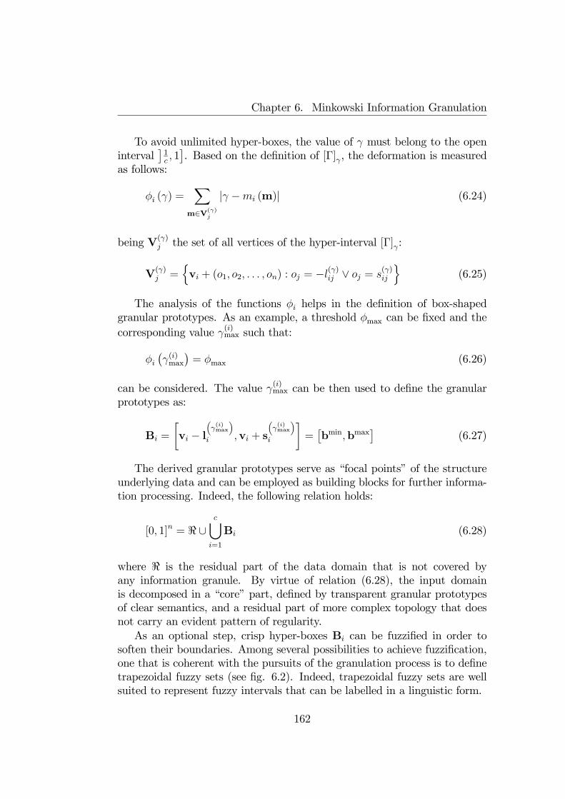
Chapter 6. Minkowski Information Granulation
To avoid unlimited hyper-boxes, the value of γ must belong to the openinterval
¤1c, 1¤. Based on the definition of [Γ]γ, the deformation is measured
as follows:
φi (γ) =X
m∈V(γ)j
|γ −mi (m)| (6.24)
being V(γ)j the set of all vertices of the hyper-interval [Γ]γ:
V(γ)j =
nvi + (o1, o2, . . . , on) : oj = −l(γ)ij ∨ oj = s
(γ)ij
o(6.25)
The analysis of the functions φi helps in the definition of box-shapedgranular prototypes. As an example, a threshold φmax can be fixed and thecorresponding value γ(i)max such that:
φi¡γ(i)max
¢= φmax (6.26)
can be considered. The value γ(i)max can be then used to define the granularprototypes as:
Bi =
·vi − l
γ(i)max
i ,vi + sγ(i)max
i
¸=£bmin,bmax
¤(6.27)
The derived granular prototypes serve as “focal points” of the structureunderlying data and can be employed as building blocks for further informa-tion processing. Indeed, the following relation holds:
[0, 1]n = < ∪c[
i=1
Bi (6.28)
where < is the residual part of the data domain that is not covered byany information granule. By virtue of relation (6.28), the input domainis decomposed in a “core” part, defined by transparent granular prototypesof clear semantics, and a residual part of more complex topology that doesnot carry an evident pattern of regularity.As an optional step, crisp hyper-boxes Bi can be fuzzified in order to
soften their boundaries. Among several possibilities to achieve fuzzification,one that is coherent with the pursuits of the granulation process is to definetrapezoidal fuzzy sets (see fig. 6.2). Indeed, trapezoidal fuzzy sets are wellsuited to represent fuzzy intervals that can be labelled in a linguistic form.
162

6.2. A method for Information Granulation through Minkowski fuzzyclustering
a b c d0
1
Figure 6.2: Shape of trapezoidal fuzzy set. The fuzzy set is well suited torepresent the fuzzy interval with core [b, c]
The parametric definition of a one dimensional trapezoidal fuzzy set isthe following:
µtrap (x; [a, b, c, d]) =
0 if x < a ∨ x > dx− a
b− aif b ≤ x ≤ c
1 if b < x < cx− d
c− dif c ≤ x ≤ d
(6.29)
LetBi be a granular prototype defined as in (6.27). It can be convenientlyrepresented as a Cartesian product of its one-dimensional projections:
Bi = Bi1 × · · · ×Bin (6.30)
being each Bij defined as:
Bij =£bminij , bmaxij
¤(6.31)
Each interval Bij can be fuzzified by defining a proper trapezoidal fuzzyset eBij with membership function
µBij(xj) = µtrap
¡xj;£aij, b
minij , bmaxij , dij
¤¢(6.32)
The parameters aij and dij can be determined according to different ap-proaches e.g. by setting them so that the support of each eBij includes all
163
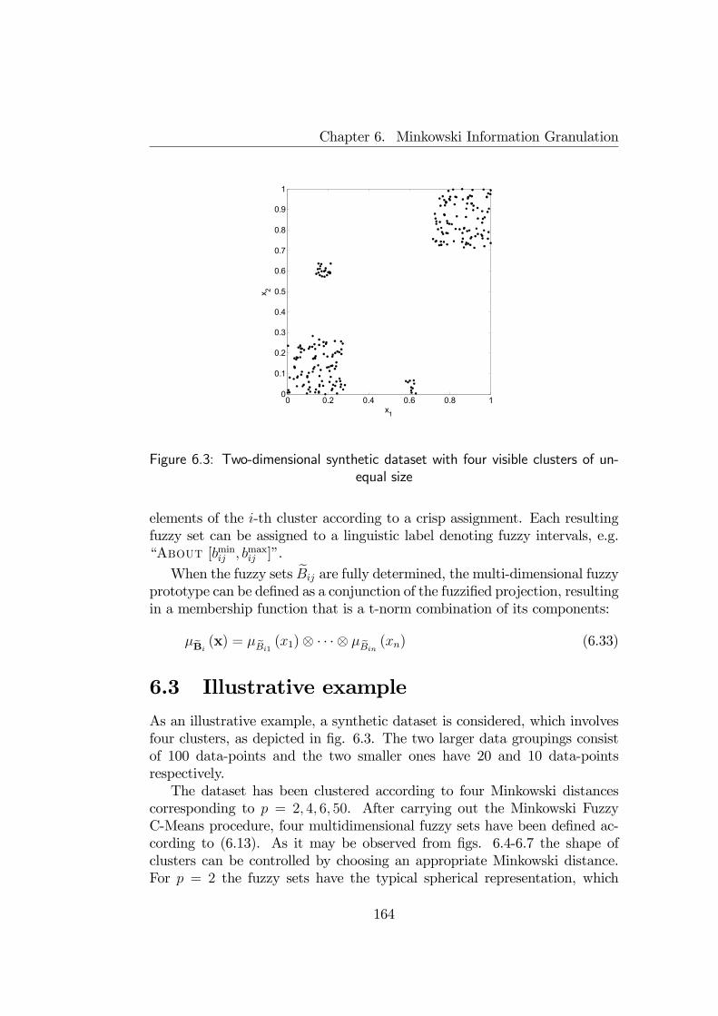
Chapter 6. Minkowski Information Granulation
0 0.2 0.4 0.6 0.8 10
0.1
0.2
0.3
0.4
0.5
0.6
0.7
0.8
0.9
1
x1
x 2
Figure 6.3: Two-dimensional synthetic dataset with four visible clusters of un-equal size
elements of the i-th cluster according to a crisp assignment. Each resultingfuzzy set can be assigned to a linguistic label denoting fuzzy intervals, e.g.“About [bminij , bmaxij ]”.When the fuzzy sets eBij are fully determined, the multi-dimensional fuzzy
prototype can be defined as a conjunction of the fuzzified projection, resultingin a membership function that is a t-norm combination of its components:
µBi(x) = µBi1
(x1)⊗ · · ·⊗ µBin(xn) (6.33)
6.3 Illustrative example
As an illustrative example, a synthetic dataset is considered, which involvesfour clusters, as depicted in fig. 6.3. The two larger data groupings consistof 100 data-points and the two smaller ones have 20 and 10 data-pointsrespectively.The dataset has been clustered according to four Minkowski distances
corresponding to p = 2, 4, 6, 50. After carrying out the Minkowski FuzzyC-Means procedure, four multidimensional fuzzy sets have been defined ac-cording to (6.13). As it may be observed from figs. 6.4-6.7 the shape ofclusters can be controlled by choosing an appropriate Minkowski distance.For p = 2 the fuzzy sets have the typical spherical representation, which
164
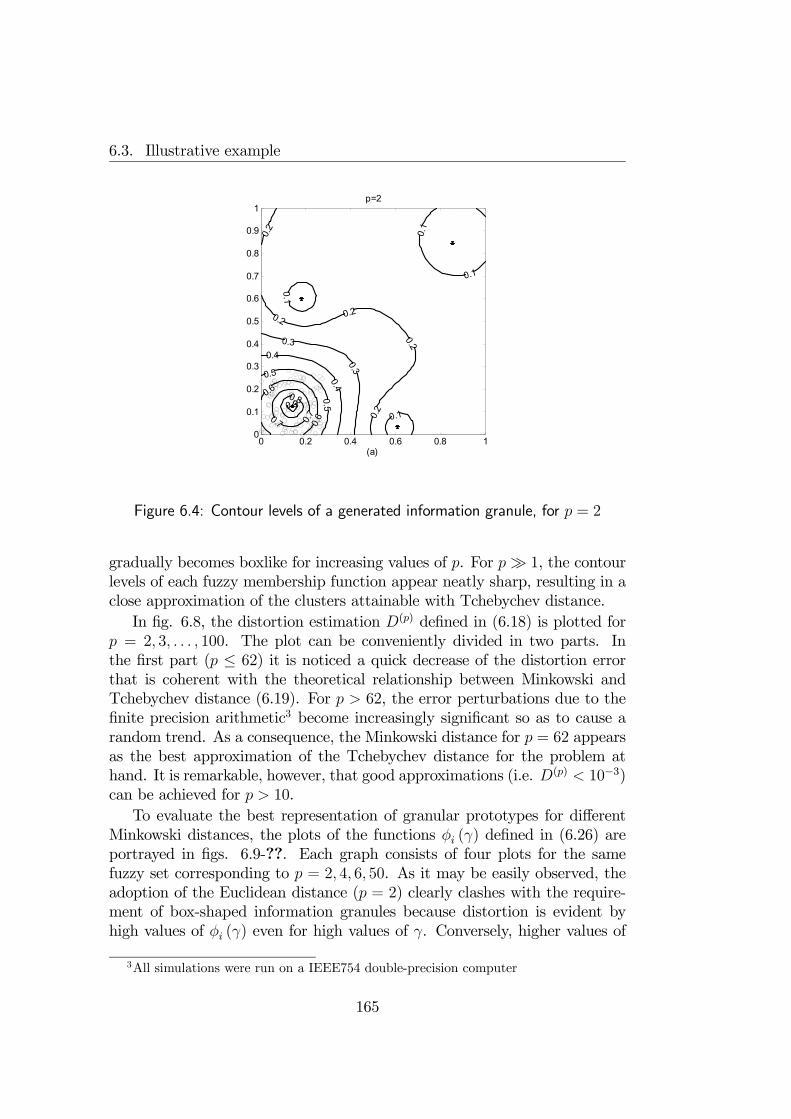
6.3. Illustrative example
0 0.2 0.4 0.6 0.8 10
0.1
0.2
0.3
0.4
0.5
0.6
0.7
0.8
0.9
1
(a)
p=2
0.1
0.1
0.1
0.1
0.2 0.2
0.20.
2
0.2
0.3
0.3
0.4
0.4
0.5
0.5
0.6
0.60.70.7
0.80.9
Figure 6.4: Contour levels of a generated information granule, for p = 2
gradually becomes boxlike for increasing values of p. For pÀ 1, the contourlevels of each fuzzy membership function appear neatly sharp, resulting in aclose approximation of the clusters attainable with Tchebychev distance.In fig. 6.8, the distortion estimation D(p) defined in (6.18) is plotted for
p = 2, 3, . . . , 100. The plot can be conveniently divided in two parts. Inthe first part (p ≤ 62) it is noticed a quick decrease of the distortion errorthat is coherent with the theoretical relationship between Minkowski andTchebychev distance (6.19). For p > 62, the error perturbations due to thefinite precision arithmetic3 become increasingly significant so as to cause arandom trend. As a consequence, the Minkowski distance for p = 62 appearsas the best approximation of the Tchebychev distance for the problem athand. It is remarkable, however, that good approximations (i.e. D(p) < 10−3)can be achieved for p > 10.To evaluate the best representation of granular prototypes for different
Minkowski distances, the plots of the functions φi (γ) defined in (6.26) areportrayed in figs. 6.9-??. Each graph consists of four plots for the samefuzzy set corresponding to p = 2, 4, 6, 50. As it may be easily observed, theadoption of the Euclidean distance (p = 2) clearly clashes with the require-ment of box-shaped information granules because distortion is evident byhigh values of φi (γ) even for high values of γ. Conversely, higher values of
3All simulations were run on a IEEE754 double-precision computer
165
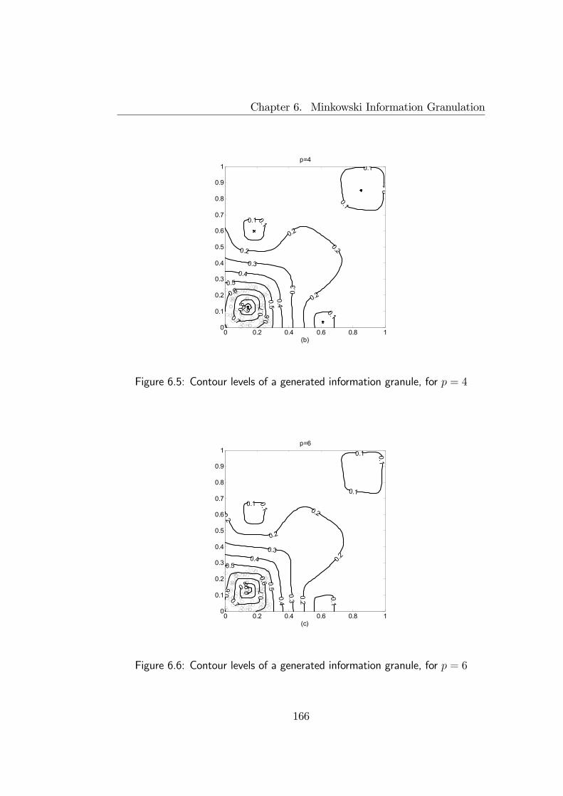
Chapter 6. Minkowski Information Granulation
0 0.2 0.4 0.6 0.8 10
0.1
0.2
0.3
0.4
0.5
0.6
0.7
0.8
0.9
1
(b)
p=4
0.1
01
0.1
0.1
0.10.1
0.2
0.20.2
0.2
0.3
0.3
0.40.4
0.50.5
0.6
0.60.
7
0.7
0.80.9
Figure 6.5: Contour levels of a generated information granule, for p = 4
0 0.2 0.4 0.6 0.8 10
0.1
0.2
0.3
0.4
0.5
0.6
0.7
0.8
0.9
1
(c)
p=6
0.1
0.1
0.1
0.1
0.10.1
0.2
0.2
0.2
0.2
0.2
0.3
0.3
0.4
0.4
0.5
0.5
0.6
0.6
0.7
0.7
0.8
0.9
Figure 6.6: Contour levels of a generated information granule, for p = 6
166
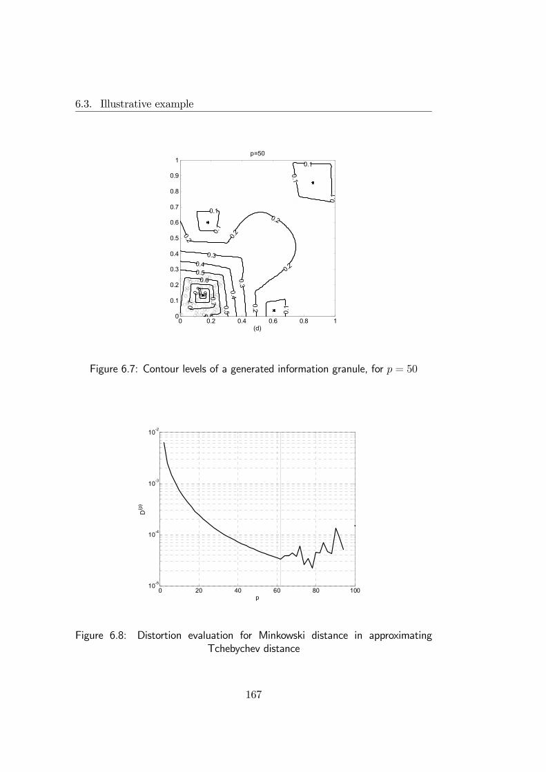
6.3. Illustrative example
0 0.2 0.4 0.6 0.8 10
0.1
0.2
0.3
0.4
0.5
0.6
0.7
0.8
0.9
1
(d)
p=50
0.1
0.1
0.1
0.1
0.1
0.1
0.2 0.2
0.2
0.2
0.2
0.3
0.3
0.4
0.4
0.5
0.5
0.6
0 6
0.7
0.7
0.80.9
Figure 6.7: Contour levels of a generated information granule, for p = 50
0 20 40 60 80 10010-5
10-4
10-3
10-2
p
D(p
)
Figure 6.8: Distortion evaluation for Minkowski distance in approximatingTchebychev distance
167

Chapter 6. Minkowski Information Granulation
0.3 0.4 0.5 0.6 0.7 0.8 0.9 10
0.1
0.2
0.3
0.4
0.5
0.6
granule 1
γ
φ i( γ)
p=2p=4p=6p=50
Figure 6.9: The plot of φ1 vs. γ
p determine very similar behavior, which is roughly characterized by a con-vex trend. Indeed, for γ ≈ 1, interactions amongst clusters is not relevant,thus the distortion value φi (γ) is close to zero. As γ decreases, the influenceof each information granule becomes significant so that the distortion valueraises consequently. For small values of γ, i.e. γ ≈ 1
c, the distortion measure
becomes small since the membership value of each fuzzy set is asymptoti-cally constant for large distances. Such behavior suggests to select the valueof γ approximately within the range [0.7, 1] to extract meaningful granularprototypes.
To derive crisp granular prototypes, the maximum distortion measure hasbeen set to φmax = 0.1. Based on such threshold, the granular prototypescorresponding to each cluster have been derived for p = 2 and p = 50 andrepresented in fig. 6.13. As it may be observed, hyper-boxes derived for p = 2appear too narrow, especially for the two biggest clusters, thus excluding asignificant number of patterns. Conversely, hyper-boxes derived for p = 50better capture the underlying structure of data. As an optional step, theresulting hyper-boxes can be fuzzified in order to provide a description ofdata in terms of soft intervals.
168

6.3. Illustrative example
0.3 0.4 0.5 0.6 0.7 0.8 0.9 10
0.1
0.2
0.3
0.4
0.5
0.6
0.7
γ
φ i( γ)
granule 2
p = 2p = 4p = 6p = 50
Figure 6.10: The plot of φ2 vs. γ
0.3 0.4 0.5 0.6 0.7 0.8 0.9 10
0.1
0.2
0.3
0.4
0.5
0.6
0.7
γ
φ i( γ)
granule 3
p = 2p = 4p = 6p = 50
Figure 6.11: The plot of φ3 vs. γ
169

Chapter 6. Minkowski Information Granulation
0.3 0.4 0.5 0.6 0.7 0.8 0.9 10
0.1
0.2
0.3
0.4
0.5
0.6
γ
φ i( γ)
granule 4
p = 2p = 4p = 6p = 50
Figure 6.12: The plot of φ4 vs. γ
0 0.2 0.4 0.6 0.8 10
0.2
0.4
0.6
0.8
x1
x 2
Figure 6.13: Granular prototypes generated for p = 2 (dashed boxes) and p = 50(solid boxes) with φmax = 0.1
170
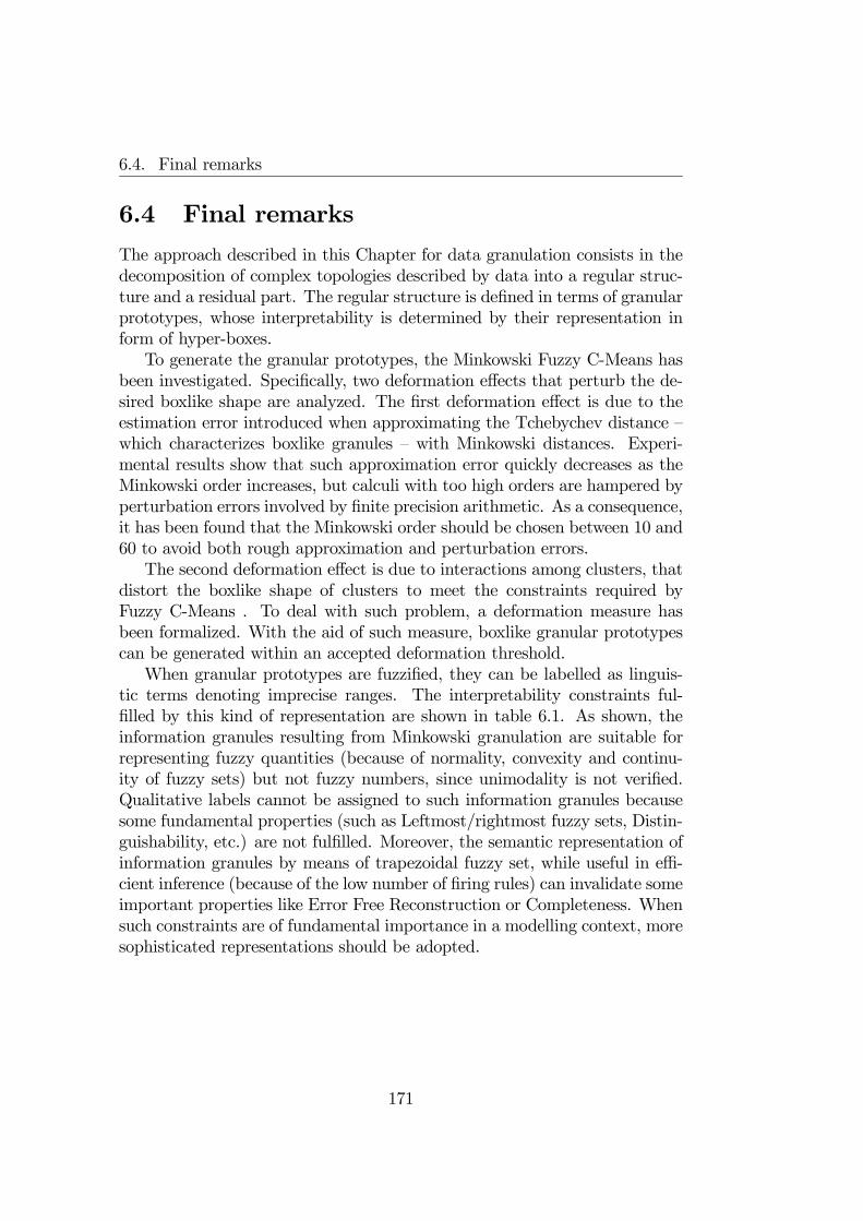
6.4. Final remarks
6.4 Final remarks
The approach described in this Chapter for data granulation consists in thedecomposition of complex topologies described by data into a regular struc-ture and a residual part. The regular structure is defined in terms of granularprototypes, whose interpretability is determined by their representation inform of hyper-boxes.To generate the granular prototypes, the Minkowski Fuzzy C-Means has
been investigated. Specifically, two deformation effects that perturb the de-sired boxlike shape are analyzed. The first deformation effect is due to theestimation error introduced when approximating the Tchebychev distance —which characterizes boxlike granules — with Minkowski distances. Experi-mental results show that such approximation error quickly decreases as theMinkowski order increases, but calculi with too high orders are hampered byperturbation errors involved by finite precision arithmetic. As a consequence,it has been found that the Minkowski order should be chosen between 10 and60 to avoid both rough approximation and perturbation errors.The second deformation effect is due to interactions among clusters, that
distort the boxlike shape of clusters to meet the constraints required byFuzzy C-Means . To deal with such problem, a deformation measure hasbeen formalized. With the aid of such measure, boxlike granular prototypescan be generated within an accepted deformation threshold.When granular prototypes are fuzzified, they can be labelled as linguis-
tic terms denoting imprecise ranges. The interpretability constraints ful-filled by this kind of representation are shown in table 6.1. As shown, theinformation granules resulting from Minkowski granulation are suitable forrepresenting fuzzy quantities (because of normality, convexity and continu-ity of fuzzy sets) but not fuzzy numbers, since unimodality is not verified.Qualitative labels cannot be assigned to such information granules becausesome fundamental properties (such as Leftmost/rightmost fuzzy sets, Distin-guishability, etc.) are not fulfilled. Moreover, the semantic representation ofinformation granules by means of trapezoidal fuzzy set, while useful in effi-cient inference (because of the low number of firing rules) can invalidate someimportant properties like Error Free Reconstruction or Completeness. Whensuch constraints are of fundamental importance in a modelling context, moresophisticated representations should be adopted.
171

Chapter 6. Minkowski Information Granulation
Table 6.1: Table of fufillment of interpretability constraints by Minkowski Gran-ulation (only applicable constraints are shown).Interpretability constraints fulfillmentNormality YesConvexity YesUnimodality NoContinuity YesProper ordering NoJustifiable no. of elements YesDistinguishability NoCompleteness NoUniform granulation NoLeftmost/Rightmost fuzzy sets NoNatural zero positioning NoError Free Reconstruction NoDescription length NoRule length NoNumber of rules LowNumber of firing rules LowShared fuzzy sets NoModel completeness No
172
Chapter 7
Information Granulationthrough Prediction Intervals
7.1 Introduction
Fuzzy information granulation is one of the basic tasks in designing fuzzymodels for solving predictive tasks. From a functional point of view, a fuzzymodel defines a pointwise input/output mapping that provides a predictionof the output value when an input is presented to the system. Differentlyfrom other predictive models, fuzzy models have the added value of an in-terpretable knowledge base that explains the functional mapping by meansof cause/effect rules. For this particularly appreciable feature, fuzzy modelshave met considerable success in control (Farinwata et al., 2000), engineering(Ross, 1997) as well as other theoretical and applicative areas. However, asalready observed in Chapter 2, interpretability is not granted by the simpleadoption of a fuzzy information granulation process to design fuzzy models,but a number of interpretability constraints have to be fulfilled.A fuzzy information granulation process that verifies all the required in-
terpretability constraints may not be sufficient to design an interpretablefuzzy model. Indeed, there are some constraints that do not depend on thegranulation technique because they involve the representation of each singlerule or the behavior of the entire model. In addition, interpretability mustbe balanced with accuracy as they are conflicting properties of a fuzzy modelthat must be equilibrated on the basis of practical issues.One of the most important interpretability constraints is the compactness
of the model, which is directly related to the number of rules that constituteits knowledge base. However, in many real-world problems, data are cor-rupted by noise or follow complex relationships that are hardly discovered
173
Chapter 7. Information Granulation through Prediction Intervals
by simple models; in such cases, a model that provides a granular output -i.e. an aggregate of values rather than a single numerical value — is moreappreciable. Prediction intervals as outputs are desirable since they providea range of values that most likely include the true value to be predicted.Moreover, prediction intervals allow the user to perceive the accuracy of theestimation provided by the model, thus deciding to keep or reject the result.The integration of prediction intervals within function approximation
models has been extensively analyzed in the neural paradigm. In (Dybowskiand Roberts, 2001; Papadopoulos et al., 2001; Ungar et al., 1996) sometechniques are critically reviewed. Unfortunately, most of the proposed ap-proaches have features that are not suitable for fuzzy models. In particular,many techniques (Nix and Weigen, 1994; Heskes, 1997; Efron and Tibshirani,1993) yield prediction intervals with length related to the input variables.While this feature can be desirable for black-box models like classical neuralnetworks, it can hamper the interpretability of the knowledge base in a fuzzymodel. Moreover, as such techniques are based on the model’s gradient,they are dependent on specific architecture and must be completely rede-fined whenever the architecture of the network changes. This is undesirablein fuzzy models — eventually encoded as neuro-fuzzy networks1 (Jang andSun, 1995)— since they are susceptible to architecture changes due to somemodification of the represented rules, e.g. by adding/deleting new rules ornew input variables. Finally, in other approaches like in (MacKay, 1992;Neal, 1996), the Bayesian framework is considered and the free parametersof the network are estimated by Monte Carlo methods. However such ap-proach is inefficient and requires strict assumptions on the free parametersthat are often impractical to solve real-world problems.In this Chapter, an approach is proposed to derive prediction intervals
for fuzzy models that in this way provide an estimate of the uncertaintyassociated with predicted output values. The derived intervals are constantthroughout the input domain and do not require any strict assumption on theunknown distribution of data. Prediction intervals can be attached to eachrule so as to provide a granulated output that enhances their interpretability.The resulting prediction intervals, even if expectably wider than those ob-
1A neuro-fuzzy network is a fuzzy model that uses a learning algorithm derived fromor inspired by neural network theory to determine its parameters (fuzzy sets and fuzzyrules) by processing data samples (Nauck et al., 1997). The key advantage of neuro-fuzzynetworks consists in their ability to acquire knowledge directly from data and representit in form of linguistically sound fuzzy rules. Compared with classical neural networks,neuro-fuzzy systems exhibit similar performances in terms of accuracy and learning speed,but their added value lies in the representation of the acquired knowledge in terms ofinterpretable fuzzy rules.
174

7.2. A method of Information Granulation through Prediction Intervals
tained with classical methods, provide a better understanding on the model’saccuracy due to their integration in the knowledge base. In addition, as themode structure changes, prediction intervals can be recomputed effortlessly.In the next section, a method of information granulation through pre-
diction interval derivation is introduced, together with a description of theirintegration in the knowledge base of a referential fuzzy model. In Section7.3, some experimental results are drawn, both from a synthetic problem andfrom a real-world problem of ash combustion prediction. The Chapter endswith some final remarks.
7.2 Amethod of Information Granulation throughPrediction Intervals
In this Section, the proposed method of information granulation throughprediction is described in detail. First, a fuzzy model is established as a ref-erence for the formalization of the method. Then, the derivation of predictionintervals is formalized and analyzed in the context of fuzzy modelling.
7.2.1 Reference Model
The pilot fuzzy model for prediction interval derivation is defined by 0thorder Takagi-Sugeno rules, which have the following schema:
Ri : IF Anti THEN y=ai (7.1)
being i = 1, 2, . . . , R. Here, Anti is an information granule resultingfrom an information granulation process and is semantically represented bya multidimensional fuzzy set Ai ∈ F (U), being U ⊆ Rn. Given a numericalinput x ∈ U, the output of the model is computed according to the followinginference formula:
y =
RPi=1
aiµAi(x)
RPi=1
µAi(x)
(7.2)
Usually, the consequent parameters ai are not evaluated by the the infor-mation granulation procedure, but through several possible techniques, in-cluding neural learning (Jang, 1993). In this latter case, the training process,may also involve the adaption of the fuzzy sets in the rule antecedents so asto minimize a given loss function, usually the Mean Squared Error.
175

Chapter 7. Information Granulation through Prediction Intervals
7.2.2 Prediction interval derivation
It is supposed that there exists a supervisor that provides, for each input x,the value y of an underlying unknown function:
y = f (x) + ε (7.3)
where f (x) is a deterministic input/output relationship and ε is a randomvariation. Random variation can be due to noise or inadequacy of the inputvariable x in fully describing the input/output relationship. Unlike otherworks known in literature, it is not assumed a zero mean value for ε. Dataprovided by the supervisor are limited to a finite training set of independentand identically distributed samples:
T =©(xp, yp) ∈ Rn+1, p = 1, 2, . . . , N
ª(7.4)
It is also assumed that the supervisor is memory-less, that is, the returnedvalue is independent on the previously calculated values. A fuzzy model isdesigned and trained so as to provide an approximated value y for the sameinput x. The following error function can be hence defined as:
e (x) = y (x)− y (x) (7.5)
After training, a finite number of errors e1, e2, . . . , eN are available. Sucherrors can be considered as independent and identically distributed univariaterandom variables with mean value:
e =1
N
NXi=1
ei (7.6)
For sampled errors, prediction intervals can be calculated. A predictioninterval [Lα, Uα] of confidence level α represents an interval that will includethe error enew of a newly drawn example xnew, with probability greater than1− α (Neter et al., 1985). Formally:
P (enew ∈ [Lα, Uα]) > 1− α (7.7)
With simple formal transformations, it is possible to derive the followinginequality:
P (y ∈ [y − Uα, y − Lα]) > 1− α (7.8)
Relation (7.8) defines a statistical method to estimate the true value ofthe underlying function approximated by the fuzzy model, with a desirable
176

7.2. A method of Information Granulation through Prediction Intervals
confidence level. Formally, a prediction interval is defined by the followingrelations:
Lα = e− tα2,[N−1]
Ãs
r1
N+ 1
!(7.9)
Uα = e+ tα2,[N−1]
Ãs
r1
N+ 1
!(7.10)
where tα2,[N−1] is the value of the Student distribution with N −1 degrees
of freedom corresponding to the critical value α/2, and s is the sampledstandard deviation:
s =
vuuut NPi=1
(ei−e)2
N − 1 (7.11)
The width of the prediction interval is directly related to the model accuracy.As a consequence, the less accurate is the model, or the smaller is the trainingset cardinality, the wider is the prediction interval.In the proposed approach, the prediction intervals are derived on the
basis of the approximated outputs inferred by the fuzzy model. However, forrepresentation pursuits, prediction intervals can be calculated for each ruleconsequent, resulting in the following representation:
IFx isAiTHEN y is in [ai − Ui,α, ai − Li,α] (1− α)% (7.12)
The individual prediction intervals are calculated by assuming each ruleto be a simple fuzzy model with input/output mapping:
yi (x) = µAi(x) · ai (7.13)
Each prediction interval is derived according to (7.5) through (7.10). Asa consequence, the knowledge base is enriched with granular outputs thatconvey information on the accuracy of each rule. Moreover, the calculationof prediction intervals for the fuzzy rules leads to a more interpretable knowl-edge base, since it helps users to perceive an entire range of validity of eachrule, instead of a single numerical value. It should be noted, however, thatsuch intervals are used only for rules representation, while the derivation ofthe prediction interval for the model output must follow relation (7.8). Thisis due to the normalization effect existing in (7.2), while direct computationof the final prediction interval from the prediction intervals of each rule ispossible only if the constraint ∀x : PR
i=1 µAi(x) = 1 is added in the design
of the fuzzy model.
177
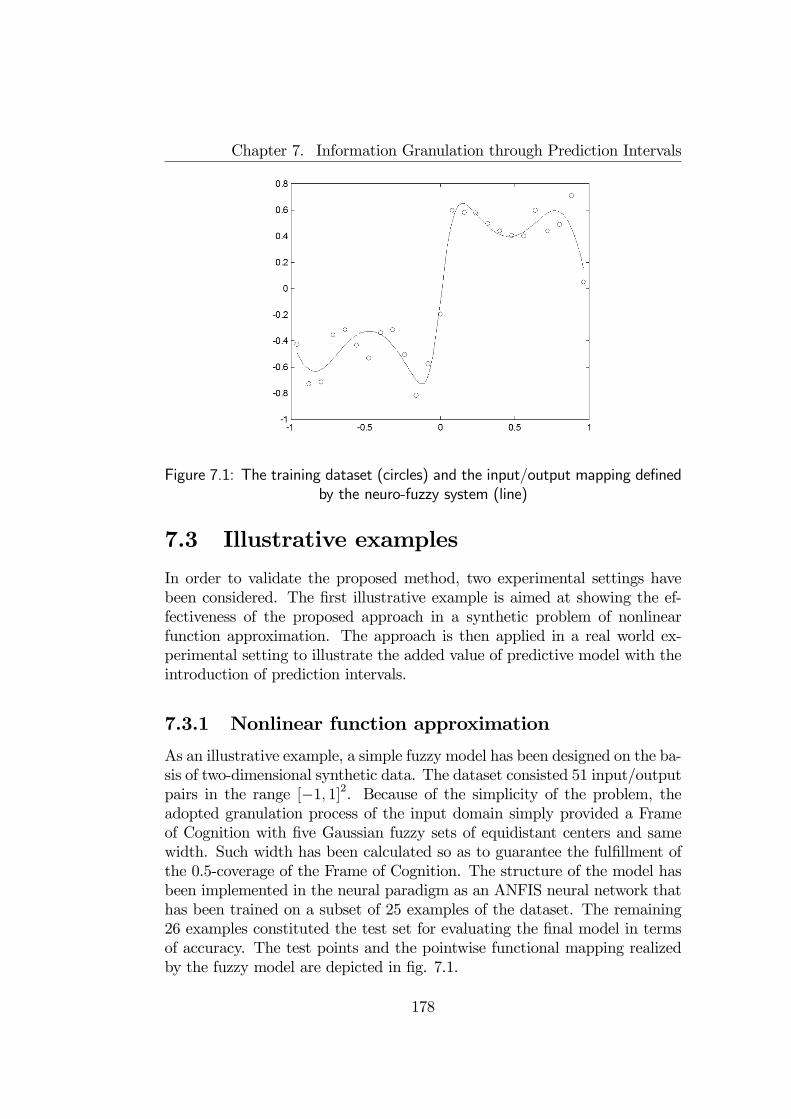
Chapter 7. Information Granulation through Prediction Intervals
Figure 7.1: The training dataset (circles) and the input/output mapping definedby the neuro-fuzzy system (line)
7.3 Illustrative examples
In order to validate the proposed method, two experimental settings havebeen considered. The first illustrative example is aimed at showing the ef-fectiveness of the proposed approach in a synthetic problem of nonlinearfunction approximation. The approach is then applied in a real world ex-perimental setting to illustrate the added value of predictive model with theintroduction of prediction intervals.
7.3.1 Nonlinear function approximation
As an illustrative example, a simple fuzzy model has been designed on the ba-sis of two-dimensional synthetic data. The dataset consisted 51 input/outputpairs in the range [−1, 1]2. Because of the simplicity of the problem, theadopted granulation process of the input domain simply provided a Frameof Cognition with five Gaussian fuzzy sets of equidistant centers and samewidth. Such width has been calculated so as to guarantee the fulfillment ofthe 0.5-coverage of the Frame of Cognition. The structure of the model hasbeen implemented in the neural paradigm as an ANFIS neural network thathas been trained on a subset of 25 examples of the dataset. The remaining26 examples constituted the test set for evaluating the final model in termsof accuracy. The test points and the pointwise functional mapping realizedby the fuzzy model are depicted in fig. 7.1.
178

7.3. Illustrative examples
Figure 7.2: Prediction intervals of the input/output mapping for four confidencelevels (10%, 1%, 0.5%, 0.1%)
Table 7.1: Prediction errors with different confidence levelsConfidence level Examples outside the prediction interval10% 2 (7.69%)1% 1 (3.85%)0.5% 00.1% 0
The proposed approach for deriving prediction intervals has been appliedon the fuzzy model acquired through ANFIS learning. More specifically, fourprediction intervals have been calculated in correspondence to the confidencelevels α = 10%, 1%, 0.5%, 0.1%. The interval mappings provided by theresulting four fuzzy models are illustrated in fig. 7.2.For each value of the confidence level, the test set has been used to check
whether the desired outputs fall within the prediction interval. The resultsare reported in table 7.1. As it can be seen, the number of desired outputsthat fall outside the prediction interval is coherent with the confidence level.In the design phase, the choice of the appropriate value of the confidence levelshould be a trade-off between precision of the mapping (narrow intervals) andgood predictive estimation (large intervals).
179
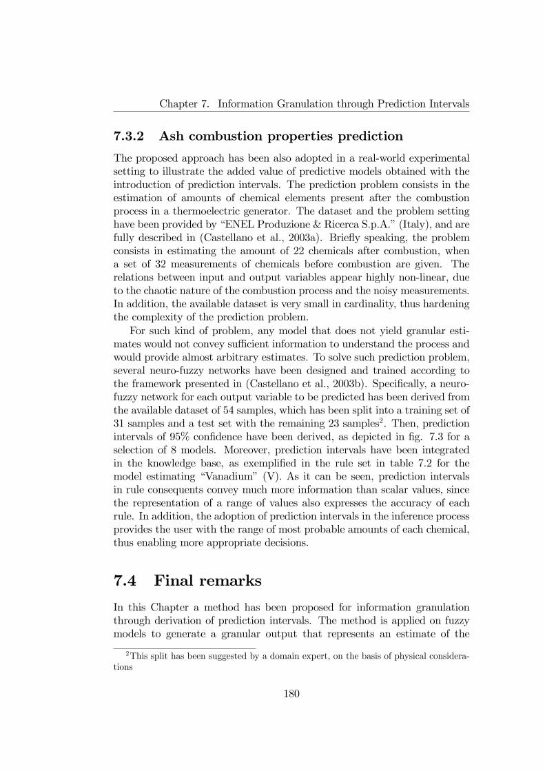
Chapter 7. Information Granulation through Prediction Intervals
7.3.2 Ash combustion properties prediction
The proposed approach has been also adopted in a real-world experimentalsetting to illustrate the added value of predictive models obtained with theintroduction of prediction intervals. The prediction problem consists in theestimation of amounts of chemical elements present after the combustionprocess in a thermoelectric generator. The dataset and the problem settinghave been provided by “ENEL Produzione & Ricerca S.p.A.” (Italy), and arefully described in (Castellano et al., 2003a). Briefly speaking, the problemconsists in estimating the amount of 22 chemicals after combustion, whena set of 32 measurements of chemicals before combustion are given. Therelations between input and output variables appear highly non-linear, dueto the chaotic nature of the combustion process and the noisy measurements.In addition, the available dataset is very small in cardinality, thus hardeningthe complexity of the prediction problem.For such kind of problem, any model that does not yield granular esti-
mates would not convey sufficient information to understand the process andwould provide almost arbitrary estimates. To solve such prediction problem,several neuro-fuzzy networks have been designed and trained according tothe framework presented in (Castellano et al., 2003b). Specifically, a neuro-fuzzy network for each output variable to be predicted has been derived fromthe available dataset of 54 samples, which has been split into a training set of31 samples and a test set with the remaining 23 samples2. Then, predictionintervals of 95% confidence have been derived, as depicted in fig. 7.3 for aselection of 8 models. Moreover, prediction intervals have been integratedin the knowledge base, as exemplified in the rule set in table 7.2 for themodel estimating “Vanadium” (V). As it can be seen, prediction intervalsin rule consequents convey much more information than scalar values, sincethe representation of a range of values also expresses the accuracy of eachrule. In addition, the adoption of prediction intervals in the inference processprovides the user with the range of most probable amounts of each chemical,thus enabling more appropriate decisions.
7.4 Final remarks
In this Chapter a method has been proposed for information granulationthrough derivation of prediction intervals. The method is applied on fuzzymodels to generate a granular output that represents an estimate of the
2This split has been suggested by a domain expert, on the basis of physical considera-tions
180

7.4. Final remarks
If Cu is in [240, 540]0.5, V is in [0, 1100]0.5, DRAWINGis in S1, S2, S3, Then V is in [0, 711] (95%);If Cu is in [220, 350]0.5, V is in [1700, 3400]0.5, DRAWINGis in S2, S3, S4, S5, Then V is in [2720, 3890] (95%);If Cu is in [260, 540]0.5, V is in [1600, 3300]0.5, DRAWINGis in S2, S3, Then V is in [1640, 2800] (95%);If Cu is in [260, 540]0.5, V is in [1600, 3300]0.5, DRAWINGis in S2, S3, Then V is in [1640, 2800] (95%);If Cu is in [0, 210]0.5, V is in [1100, 2900]0.5, DRAWINGis in S1, S2, Then V is in [1140, 2310] (95%);If Cu is in [0, 260]0.5, V is in [0, 1400]0.5, DRAWINGis in S2, S3, S4, S5, Then V is in [0, 877] (95%);If Cu is in [290, 590]0.5, V is in [950, 1710]0.5, DRAWINGis in S4, S5, Then V is in [1590, 2750] (95%);If Cu is in [0, 290]0.5, V is in [0, 1400]0.5, DRAWINGis in S1, S2, S3, Then V is in [0, 690] (95%)
Table 7.2: The ruleset generated for predicting Vanadium after the combustionprocess, on the basis of the quantitis of Copper (Cu) and Vanadium (V) beforecombustion, and the drawing source. For ease of reading, the fuzzy sets in the
rules antecedents have been represented by their respective 0.5-cuts
181
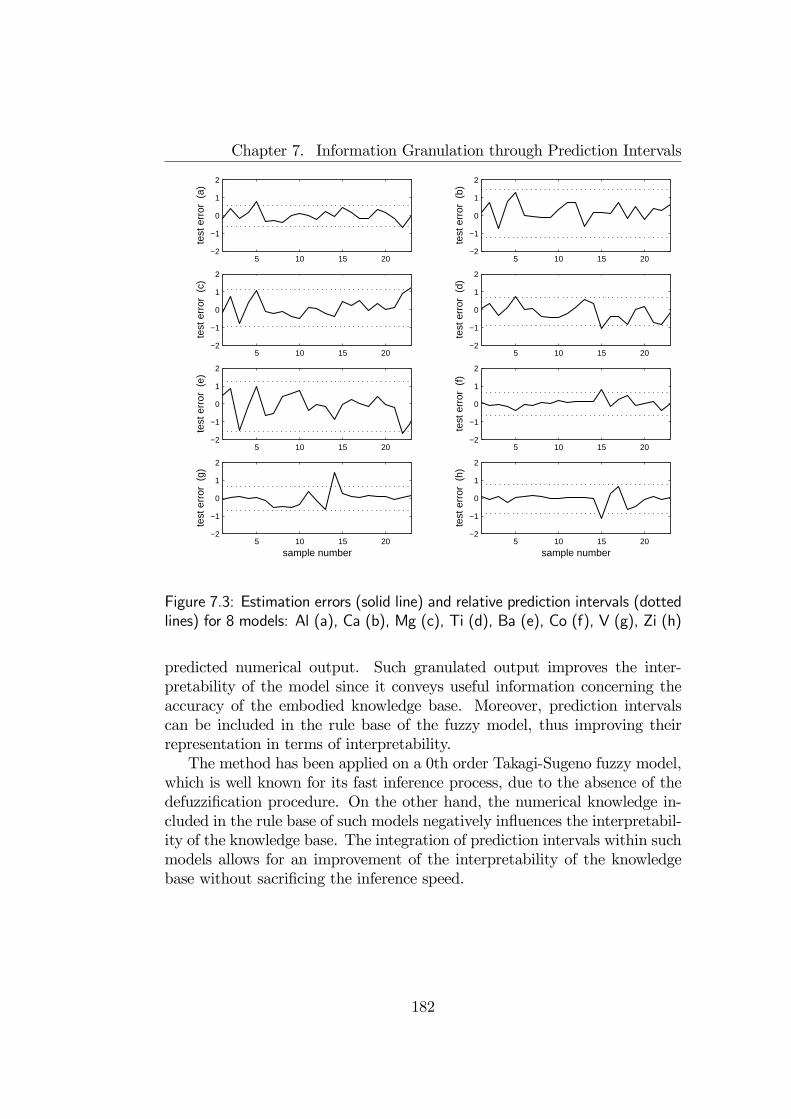
Chapter 7. Information Granulation through Prediction Intervals
5 10 15 20−2
−1
0
1
2
test
err
or (
a)
5 10 15 20−2
−1
0
1
2
test
err
or (
b)
5 10 15 20−2
−1
0
1
2
test
err
or (
c)
5 10 15 20−2
−1
0
1
2
test
err
or (
d)5 10 15 20
−2
−1
0
1
2
test
err
or (
e)
5 10 15 20−2
−1
0
1
2
test
err
or (
f)
5 10 15 20−2
−1
0
1
2
sample number
test
err
or (
g)
5 10 15 20−2
−1
0
1
2
sample number
test
err
or (
h)
Figure 7.3: Estimation errors (solid line) and relative prediction intervals (dottedlines) for 8 models: Al (a), Ca (b), Mg (c), Ti (d), Ba (e), Co (f), V (g), Zi (h)
predicted numerical output. Such granulated output improves the inter-pretability of the model since it conveys useful information concerning theaccuracy of the embodied knowledge base. Moreover, prediction intervalscan be included in the rule base of the fuzzy model, thus improving theirrepresentation in terms of interpretability.The method has been applied on a 0th order Takagi-Sugeno fuzzy model,
which is well known for its fast inference process, due to the absence of thedefuzzification procedure. On the other hand, the numerical knowledge in-cluded in the rule base of such models negatively influences the interpretabil-ity of the knowledge base. The integration of prediction intervals within suchmodels allows for an improvement of the interpretability of the knowledgebase without sacrificing the inference speed.
182

Chapter 8
Information Granulationthrough Double Clustering
8.1 Introduction
The key feature of information granulation consists in forming meaningfulpieces of information that exhibit some functional and descriptive represen-tation of data gathered into each information granule. Such a representationcould take different forms, depending on the nature of data as well as onapplicative needs.In the previous chapters, some techniques for information granulation
have been proposed, with the main objective of representing quantitativeinformation. This type of representation usually takes the form of fuzzynumber, fuzzy vector or fuzzy/probabilistic interval, and could be also usedas a basis for further arithmetic processing.In different applicative areas, however, quantitative representation of data
may not be necessary, nor helpful. In some cases, a qualitative descriptionof data, which makes use of linguistic terms like “small”, “cold”, “bright”,etc., could be more advantageous. Indeed, qualitative linguistic terms areoften used in common speech and are very helpful in conveying informationin an economic yet effective way. As a consequence, the adoption of a qual-itative representation of information granules could significantly boost theinterpretability of a knowledge base.Information granulation of data with qualitative representation requires a
higher number of interpretability constraints than in the case of quantitativerepresentation since the metaphors associated to linguistic terms are relatedtogether more tightly than for linguistic quantities. As a consequence, anumber of additional constraints is required, especially those defined at the
183
Chapter 8. Information Granulation through Double Clustering
level of Frame of Cognition1.The interpretability constraints that are essential in a sound qualitative
representation of information granules are:
• Normality, convexity, continuity, as for quantitatively represented in-formation granules;
• Proper ordering, so as to reflect the ordering of linguistic labels (e.g.“small” recalls a concept that precedes “large” w.r.t. a suitable scale);
• Justifiable number of elements, because the number of linguistic labelsused to describe an attribute is usually very limited;
• Distinguishability, because different linguistic labels designate well dis-tinct metaphors;
• Completeness, because each element of the Universe of Discourse couldbe denoted by at least one linguistic label;
• Leftmost/Rightmost fuzzy sets, which properly refer to limit cases intoa Universe of Discourse.
The process of automatically extracting information granules from datawith qualitative representation is rather difficult because it implies two majorproblems: (1) the discover of hidden relationships among multi-dimensionaldata, and (2) the representation of such relationship in terms in a linguis-tically interpretable fashion. Usually, the problem of discovering hidden re-lationships among data is tackled with cluster analysis techniques, whichhowever may fail in providing a qualitative description of data in terms ofinterpretable fuzzy information granules. On the other hand, the a-prioridefinition of interpretable fuzzy sets is relatively simple, but it is rather hardto guarantee that information granules based on such definition adequatelyrepresent the relationships underlying the distribution of data.In this Chapter, an algorithmic framework is proposed, called “Double
Clustering Framework”, which enables the extraction of qualitatively de-scribed information granules with through efficient clustering techniques.The framework is mainly centered on two clustering steps: the first, appliedon the multidimensional data, is aimed at discovering the hidden relation-ships among data, while the second, which operates at the level of each di-mension, enables the definition of interpretable fuzzy sets that can be labelled
1See Chapter 2 for a deeper discussion.
184

8.2. The Double Clustering Framework
with linguistic terms. The framework does not fully specify the clusteringalgorithms, which could be chosen according to different applicative needs.The Double Clustering Framework is described in detail in Section 8.2,
along with some implementations that include specific clustering algorithms.Then, some illustrative examples are portrayed and conclusive remarks aredrawn.
8.2 The Double Clustering Framework
The Double Clustering Framework is an algorithmic scheme that enables theextraction of fuzzy information granules representable in terms of qualitativelinguistic labels. It is made of three main steps:
1. Data Clustering. Clustering is performed in the multi-dimensionalspace of experimental data — assumed to belong to a numerical domain— to embrace similar points into granules. At this stage, the informationgranules are described by single multi-dimensional prototypes definedon the same numerical level of experimental data;
2. Prototype Clustering. The prototypes obtained from the first clus-tering stage are further clustered along each dimension of the numericaldomain, so as to obtain a number of one-dimensional prototypes on eachdimension;
3. Granule Fuzzification. Multidimensional and one-dimensional pro-totypes provide useful information to derive information granules thatcan be conveniently represents by fuzzy sets. Moreover, such fuzzy setscan be built in accord to the interpretability constraints that allow aqualitative description of the information granules.
The framework tries to exploit the features of both multi-dimensional andone-dimensional clustering. Precisely, the multi-dimensional clustering cap-tures the granularity of the data in the multi-dimensional space, but the fuzzi-fication of the resulting granules typically results in fuzzy sets that cannot beassociated with qualitative linguistic labels. Conversely, the one-dimensionalclustering can provide interpretable fuzzy sets but may loose informationabout the granularity of the multi-dimensional data. The combined applica-tion of both one-dimensional and multi-dimensional clustering exploits thebenefits of the two approaches and enables an interpretable granulation of in-formation. A schema of the process carried out within the Double ClusteringFramework is portrayed in fig. 8.1.
185

Chapter 8. Information Granulation through Double Clustering
MultidimensionalClustering
MultidimensionalData
GranuleFuzzification
One DimensionalPrototypeClustering
Information Granules
Figure 8.1: The three steps of the Double Clustering Framework
186
8.2. The Double Clustering Framework
Formally, the Double Clustering Framework can be described as follows.Let
X = [m1,M1]× · · · × [mn,Mn] ⊆ Rn (8.1)
be the n-dimensional Universe of Discourse in which an available set of nu-merical data
D = xi ∈ X : i = 1, 2, . . . , N (8.2)
is defined.The first stage of the Double Clustering Framework performs a multi-
dimensional clustering on the dataset D, providing a collection of multi-dimensional prototypes
c1, c2, . . . , cp ∈ X (8.3)
being ci =³c(1)i , c
(2)i , . . . , c
(n)i
´, i = 1, 2, ..., p.
The multi-dimensional prototypes are then projected onto each dimen-sion, resulting in n sets
C(j) =nc(j)i ∈ [mj,Mj] : i = 1, 2, . . . , p
o(8.4)
for j = 1, 2, . . . , n. The points of each C(j) are subject to one-dimensionalclustering in the second step, yielding to one-dimensional prototypes
P (j) =np(j)1 , p
(j)2 , . . . , p
(j)Kj
o(8.5)
being Kj the number of clusters in the j-th dimension, which must be low inaccordance to the “justifiable number of elements” interpretability constraint.The last stage of the Double Clustering Framework involves the fuzzifi-
cation of the information granules. This is achieved by first fuzzifying theone-dimensional granules defined by the prototypes in each P (j) and thenby aggregating one-dimensional fuzzy sets to form multi-dimensional fuzzyinformation granules.For each dimension j = 1, 2, . . . , n, the Kj extracted clusters are trans-
formed into as many interpretable fuzzy sets. Different types of membershipfunctions can be used to characterize fuzzy sets; here, Gaussian fuzzy setsare considered, with the following membership functions:
µA(j)k(x) = exp
−³x− ω
(j)k
´22³σ(j)k
´2 (8.6)
187
Chapter 8. Information Granulation through Double Clustering
for k = 1, 2, . . . ,Kj. To complete the mathematical definition of fuzzy sets,the values of the centers ω(j)k and the widths σ(j)k must be derived.The definition of such values must take into account the information pro-
vided by the clustering stages and, at the same time, must consider the re-quired interpretability constraints. To meet both requirements, the following“cut points” are defined:
t(j)k =
2mj − t
(j)1 for k = 0³
p(j)k + p
(j)k+1
´/2 for 0 < k < Kj
2Mj − t(j)Kj−1 for k = Kj
(8.7)
Note that there are Kj + 1 cut point for each dimension. Cut points canbe used to define centers and widths of the Gaussian membership functions sothat the interpretability constraints can be met. Their values can be derivedby the following relations:
ω(j)k =
t(j)k−1 + t
(j)k
2(8.8)
and
σ(j)k =
t(j)k − t
(j)k−1
2√−2 ln ε (8.9)
where ε is the maximum allowed overlap (possibility) between two adjacentfuzzy sets2.It is easy to show that for each dimension, the fuzzy sets defined in
(8.6) meet all required interpretability constraints, so qualitative linguisticlabels can be attached within the newly formed frame of cognition. Morespecifically:
• Normality, convexity and continuity are verified by the Gaussian shapeof fuzzy sets;
• Proper ordering is verified by defining the order relation of fuzzy setsreflecting the order of the prototypes.
• Justifiable number of elements is verified by an appropriate choice ofKj;
2On the basis of theoretical results derived in Chapter 3, the possibility measure is usedto quantify distinguishability
188
8.2. The Double Clustering Framework
• Distinguishability is verified by construction of the fuzzy sets, whichhave possibility measure not exceeding the allowed overlap ε;
• Completeness is verified by construction of the fuzzy sets, which guar-antee ε-coverage;
• Leftmost/Rightmost fuzzy sets by construction of the first and lastfuzzy sets, whose prototypes coincide with the limits of Universe ofDiscourse.
Once the fuzzification process is completed, for each dimension a Frame ofCognition can be defined, by attaching proper linguistic labels to the derivedfuzzy sets. Because of the verification of the interpretability constraints, theassociation of linguistic labels is a straightforward process.Let
F(j) =U (j),F(j),¹(j),L(j), v(j)® (8.10)
be the Frames of Cognition defined after the granulation process. Multi-dimensional fuzzy information granules are formed by combining one-dimen-sional fuzzy sets, one for each frame. A naïve approach, however, wouldlead to an exponentially high number of information granules, which violatesthe compactness interpretability constraint. Indeed, the total number ofinformation granules is
nYj=1
Kj ∼ Ω (2n) (8.11)
Furthermore, the so derived information granule would not convey anyuseful information concerning the distribution of data and, hence, a descrip-tion of their underlying relationships. To avoid combinatorial explosion ofmulti-dimensional fuzzy information granules, only those granules that aremost representative of the multi-dimensional prototypes ci are considered.The selection of such granules is accomplished within each dimension, byconsidering, for each i = 1, 2, . . . , p, the fuzzy set in the j-th dimension withhighest membership value on the j-th projection of the i-th prototype. Theindex of such fuzzy set is defined as:
k(j)i = argmax
k=1,2,...,Kj
µA(j)k
³c(j)i
´(8.12)
Once representative fuzzy sets are chosen, multi-dimensional fuzzy infor-mation granules can be defined as usual. Specifically, the semantics of each
189

Chapter 8. Information Granulation through Double Clustering
information granule is defined by the Cartesian product of the selected fuzzysets while its syntax is defined as:
v(1) is LµA(1)
k(j)i
¶AND . . . AND v(n) is L
µA(n)
k(n)i
¶(8.13)
for i = 1, 2, . . . , p. It is possible that two ore more information granulescoincide, hence the total number of derived granules is upper bounded bythe number of multi-dimensional prototypes p.When the granulation process is completed, a fuzzy rule-based model can
be built on the basis of the derived fuzzy granules. This is aimed to verifyhow much the fuzzy granules identified from data are useful in providinggood mapping properties or classification capabilities.The Double Clustering Framework can be customized by choosing ap-
propriate clustering algorithms, either for the multi-dimensional or the one-dimensional stage. The unique requirement for such algorithms is to producea set of prototypes in conformity with the granulation process outlined in theprevious Section.The choice of specific clustering algorithms defines an implementation of
the Double Clustering Framework, and depends on applicative issues. Inthe following, some implementations of the framework are described, andpotential applicative contexts are considered.
8.2.1 Fuzzy Double Clustering
A first implementation of the Double Clustering Framework integrates a fuzzyclustering algorithm in the first stage for multi-dimensional clustering, and ahierarchical clustering scheme for the one-dimensional clustering. This typeof implementation is particularly suited to enhance existing applications offuzzy clustering in order to enable interpretable fuzzy information granula-tion.The fuzzy clustering scheme for the first stage could be any algorithm that
carries out a set of prototypes as a result of its execution process. Examplesof such scheme are the Fuzzy C-Means (Bezdek, 1981) and all its variants, likethe Gustafson-Kessel algorithm (Gustafson and Kessel, 1979), the Gath-Gevaalgorithm (Abonyi et al., 2002), the Conditional Fuzzy C-Means (Pedrycz,1996a), etc. Also, Possibilistic C-Means can be applied (Krishnapuram andKeller, 1993), as well as other clustering schemes (Baraldi and Blonda, 1999).In the choice of a specific clustering algorithm, the maximum number of fuzzyclusters that can be extracted must be a controlled parameter; indeed anuncontrolled number of clusters may hamper the compactness requirementthat is fundamental for the interpretability of the fuzzy model. For this
190
8.2. The Double Clustering Framework
reason, fuzzy clustering algorithms that require a fixed (or maximum) numberof clusters as working parameters are preferred for the implementation of thefirst stage of the Double Clustering Framework.The second stage of one-dimensional clustering does not require a fuzzy
clustering scheme, since fuzzification in each dimension is an integral partof the Double Clustering Framework that is accomplished in its third stage.Moreover, since the number of points to be clustered coincides with thenumber of multi-dimensional clusters, and since the latter is very low toguarantee compactness of the fuzzy model, simple one-dimensional clusteringalgorithms can be adopted.Hierarchical clustering is a crisp, simple clustering algorithm that has
the additional property of being quite efficient for one-dimensional numericaldata, provided that such data are sorted. These advantageous features justifyits adoption within the considered implementation of the Double ClusteringFramework.The application of hierarchical clustering within the Double Clustering
Framework is as follows. For each dimension j = 1, 2, . . . , n, the set ofprototype projections C(j) defined in (8.4) is sorted to provide the followingarray:
−−→C(j) =
Dc(j)i1, c(j)i2, . . . , c
(j)ip
E(8.14)
such that c(j)ih ≤ c(j)ih+1.
The hierarchical clustering operates by successive partitions of−−→C(j), and
terminates when a partition of defined cardinality Kj is reached. The firstpartition is trivial, with each element of the array forming a single cluster(hereafter the index (j) is dropped for ease of notation):
H0 =h01, h
02, . . . , h
0p
®(8.15)
being
h0l = cil , l = 1, 2, . . . , p (8.16)
For the partition H0 a trivial set of prototypes is also defined as:
P 0 =p01, p
02, . . . , p
0p
®(8.17)
where
p0l = cil , l = 1, 2, . . . , p (8.18)
191
Chapter 8. Information Granulation through Double Clustering
The clustering process proceeds by aggregating clusters from previouspartitions. The clusters to be merged are chosen on the basis of the minimaldistance between prototypes. Since data are one-dimensional and sorted, theselection of the two closest clusters can be achieved within a single scan ofthe prototype array, thus resulting in a very efficient process.The aggregation process is carried out as follows. For k = 1, 2, . . . , p−Kj,
the two nearest prototypes from the (k − 1)-th partition are selected and theirposition is considered:
l∗k = argmaxl=1,2,...,p−k−1
¯pk−1l − pk−1l+1
¯(8.19)
The position index l∗k enables the definition of a new partition Hk that is
identical to Hk−1 with the exception of the clusters hk−1l∗kand hk−1l∗k+1
that aremerged together. The formal definition of Hk is given as follows:
Hk =hk1, h
k2, . . . , h
kp−k®
(8.20)
where, for each l = 1, 2, . . . , p− k:
hkl =
hk−1l if l < l∗khk−1l ∪ hk−1l+1 if l = l∗khk−1l+1 if l > l∗k
(8.21)
The new prototype array P k =pk1, p
k2, . . . , p
kp
®can be computed on the
basis of the new partition Hk:
pkl =1¯hkl¯ Xc∈hkl
c, l = 1, 2, . . . , p− k (8.22)
Prototype calculation can be simplified with the observation that thevalues of P k change from P k−1 only in one element. For k = p − Kj theclustering process is stopped and the final prototype set P (j) is defined as:
P (j) = P p−Kj (8.23)
Each cycle of the clustering process hence takes O (p− k) operations andthe number of cycles is p−Kj +1. By adding the time necessary to sort theprototypes before clustering — O (p2) in the worst case — the time complexityof the hierarchical clustering procedure for all dimensions is
O¡np2 − nK2
¢(8.24)
192
8.2. The Double Clustering Framework
being
K = maxj=1,2,...,n
Kj (8.25)
Since the number of prototypes is usually much lower that the cardinalityof the dataset D, it can be affirmed that the overhead of the Double Clus-tering Framework is negligible when compared to the time complexity of themultidimensional clustering procedure, which is usually at least linear in thecardinality of the dataset, N .
8.2.2 Crisp Double Clustering
Fuzzy Double Clustering is useful when an existing fuzzy clustering appli-cation must be wrapped so as to accommodate interpretability constraints.When new systems have to be developed, it is more convenient to use avector quantization technique in substitution to the fuzzy clustering algo-rithm in the first stage of the Double Clustering Framework. This choiceis motivated by the unnecessity of the partition matrix within the DoubleClustering Framework, which is usually calculated — with a significant timeconsumption — by fuzzy clustering algorithms.The Crisp Double Clustering is based on a general-purpose vector quanti-
zation algorithm that follows the Linde-Buzo-Gray (LBG) formulation (Lindeand Gray, 1980). From the dataset D a number of p multi-dimensional pro-totypes c01, c
02, . . . , c
0p ∈ D is randomly selected. Based on such prototypes,
the dataset D is partitioned according to:
D0l =
½x ∈ D :
°°x− c0l °° = mink=1,2,...p
°°x− c0k°°¾ (8.26)
where k·k is a suitable norm. The partition D01,D
02, . . . , D
0p is used to define
a new set of prototypes
c1l =1
|D0l |Xx∈D0
l
x, l = 1, 2, . . . , p (8.27)
The new set of prototype is used to calculate a new partition as in (8.26)and then a new set of prototypes as in (8.27). The process is repeatediteratively so as to generate a sequence of prototype vectors ckl , for k =0, 1, 2, . . .. The iterative process is stopped when a termination criterion ismet, e.g. when all prototypes do not change significantly:
STOP when ∀l = 1, 2, . . . , p : °°ckl − ck−1l
°° < (8.28)
193
Chapter 8. Information Granulation through Double Clustering
where is a user-defined threshold. An accurate implementation of the LBGalgorithm can avoid the explicit representation of the partitions Dk
l , thussaving significant amounts of memory space3.
8.2.3 DCClass
The Crisp Double Clustering implementation is general-purpose and can beapplied to all problems of numerical data granulation. However, for clas-sification problems, the information deriving from the class partitioning ofdata can be effectively exploited to improve the granulation process. Morespecifically, the class division of data can be used to automatically determinethe granularity level for each attribute, without the need of specifying thenumber Kj of fuzzy sets onto each dimension.The first stage of DCClass is similar to Crisp Double Clustering, though
better results can be achieved if a classification-oriented vector quantizationalgorithm is used in substitution to the classical LBG scheme. An exampleof algorithm that performs vector quantization in classification problems isLVQ1 (Learning Vector Quantization, version 1) (Kohonen, 1986), thoughmore stable techniques may be adopted, like Self Organizing Maps, etc.(Kohonen, 1990; Kohonen, 1997). As an example, the LVQ1 algorithm isportrayed in the following.Let DC be the dataset of numerical data enriched with class information:
DC = hxi, ψii : i = 1, 2, . . . , N ⊆ X × C (8.29)
where C is the set of all class labels
C = Ψ1,Ψ2, . . . ,Ψm (8.30)
The LVQ1 algorithm operates by firstly selecting at random a number ofp prototypes fromDC, possibly reflecting the class distribution of the dataset.This selection corresponds to the first array of prototypes:
c01, ψc1
®,c01, ψc2
®, . . . ,
c0p, ψcp
® ∈ DC (8.31)
The prototypes are then updated interactively, by selecting at randoman example
xik , ψik
®from the dataset DC and following an update rule
3This could be achieved by defining two arrays of p elements, namely COUNT[1..p]and SUM[1..p]. Each element x of D is compared to all prototypes; if the l-th prototypeis the closest, then COUNT[l]:=COUNT[l]+1 and SUM[l]:=SUM[l]+x. The new prototypesare calculated as c[l]:=SUM[l]/COUNT[l]; in this way the algorithm requires only anamount of memory proportional to 3p to compute prototypes.
194
8.2. The Double Clustering Framework
that involves only the prototype ckl that is closest to the selected point xik .The update rule takes into account the class information, so as to bring theprototype closer to the data point if the class labels coincide, and to keep theprototype away from the data point if the class labels are different. Statedformally:
ckl =
½ck−1l + αk
¡xik − ck−1l
¢if ψcl = ψik
ck−1l − αk
¡xik − ck−1l
¢if ψcl 6= ψik
(8.32)
The update iterations are repeated until a convergence criterion is met,like the one define in (8.28).A key feature of classification-oriented vector quantization algorithms is
the possibility to clearly assign a class label to each prototype. This classinformation is also inherited by the prototype projections, so that each multi-dimensional prototype can be represented as
hcl, ψcli =D³
c(1)l1 , c
(2)l2 , . . . , c
(n)ln
´, ψcl
E(8.33)
and the set of projection on the j-th dimension Cj as:
C(j) =nD
c(j)l , ψcl
E∈ [mj,Mj]× C : l = 1, 2, . . . , p
o(8.34)
By sorting each C(j) on the values c(j)l , the following array can be derived:
−−→C(j) =
DDc(j)l1, ψcl1
E,Dc(j)l2, ψcl2
E, . . . ,
Dc(j)lp, ψclp
EE(8.35)
A partition of elements of−−→C(j) is automatically induced by the class labels
ψclkby keeping in the same cluster all adjacent elements that share the same
class label. Formally, the one-dimensional projections are clustered accordingto the partition induced by the following equivalence relation:
c(j)lk≡ c
(j)lk+1⇐⇒ ψclk
= ψclk+1(8.36)
for k = 1, 2, . . . , p−1. The number of one-dimensional clusters is not defineda priori, but it is upper bounded by p. As a consequence, if p is small (to meetthe compactness requirement), also the number of clusters in each dimensionis low.For each one-dimensional cluster, one-dimensional prototypes can be cal-
culated according to (8.22), so that the fuzzy information granules can bedefined according to the Double Clustering Framework.The granulation process carried out by DCClass is graphically exemplified
in figs. 8.2—8.4. In fig. 8.2, data are quantized through the LVQ1 algorithms,
195
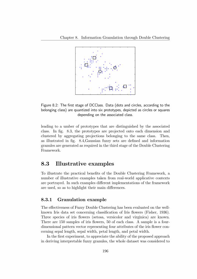
Chapter 8. Information Granulation through Double Clustering
Figure 8.2: The first stage of DCClass. Data (dots and circles, according to thebelonging class) are quantized into six prototypes, depicted as circles or squares
depending on the associated class.
leading to a umber of prototypes that are distinguished by the associatedclass. In fig. 8.3, the prototypes are projected onto each dimension andclustered by aggregating projections belonging to the same class. Then,as illustrated in fig. 8.4,Gaussian fuzzy sets are defined and informationgranules are generated as required in the third stage of the Double ClusteringFramework.
8.3 Illustrative examples
To illustrate the practical benefits of the Double Clustering Framework, anumber of illustrative examples taken from real-world applicative contextsare portrayed. In such examples different implementations of the frameworkare used, so as to highlight their main differences.
8.3.1 Granulation example
The effectiveness of Fuzzy Double Clustering has been evaluated on the well-known Iris data set concerning classification of Iris flowers (Fisher, 1936).Three species of iris flowers (setosa, versicolor and virginica) are known.There are 150 samples of iris flowers, 50 of each class. A sample is a four-dimensional pattern vector representing four attributes of the iris flower con-cerning sepal length, sepal width, petal length, and petal width.In the first experiment, to appreciate the ability of the proposed approach
in deriving interpretable fuzzy granules, the whole dataset was considered to
196
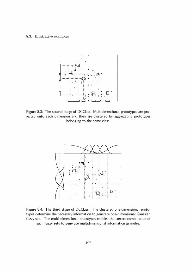
8.3. Illustrative examples
Figure 8.3: The second stage of DCClass. Multidimensional prototypes are pro-jected onto each dimension and then are clustered by aggregating prototypes
belonging to the same class.
Figure 8.4: The third stage of DCClass. The clustered one-dimensional proto-types determine the necessary information to generate one-dimensional Gaussianfuzzy sets. The multi-dimensional prototypes enables the correct combination of
such fuzzy sets to generate multidimensional information granules.
197
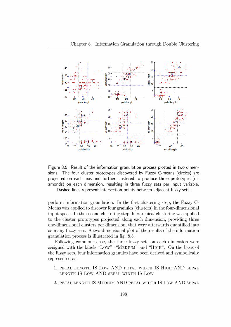
Chapter 8. Information Granulation through Double Clustering
Figure 8.5: Result of the information granulation process plotted in two dimen-sions. The four cluster prototypes discovered by Fuzzy C-means (circles) areprojected on each axis and further clustered to produce three prototypes (di-amonds) on each dimension, resulting in three fuzzy sets per input variable.
Dashed lines represent intersection points between adjacent fuzzy sets.
perform information granulation. In the first clustering step, the Fuzzy C-Means was applied to discover four granules (clusters) in the four-dimensionalinput space. In the second clustering step, hierarchical clustering was appliedto the cluster prototypes projected along each dimension, providing threeone-dimensional clusters per dimension, that were afterwards quantified intoas many fuzzy sets. A two-dimensional plot of the results of the informationgranulation process is illustrated in fig. 8.5.Following common sense, the three fuzzy sets on each dimension were
assigned with the labels “Low”, “Medium” and “High”. On the basis ofthe fuzzy sets, four information granules have been derived and symbolicallyrepresented as:
1. petal length IS Low AND petal width IS High AND sepallength IS Low AND sepal width IS Low
2. petal length IS Medium AND petal width IS Low AND sepal
198
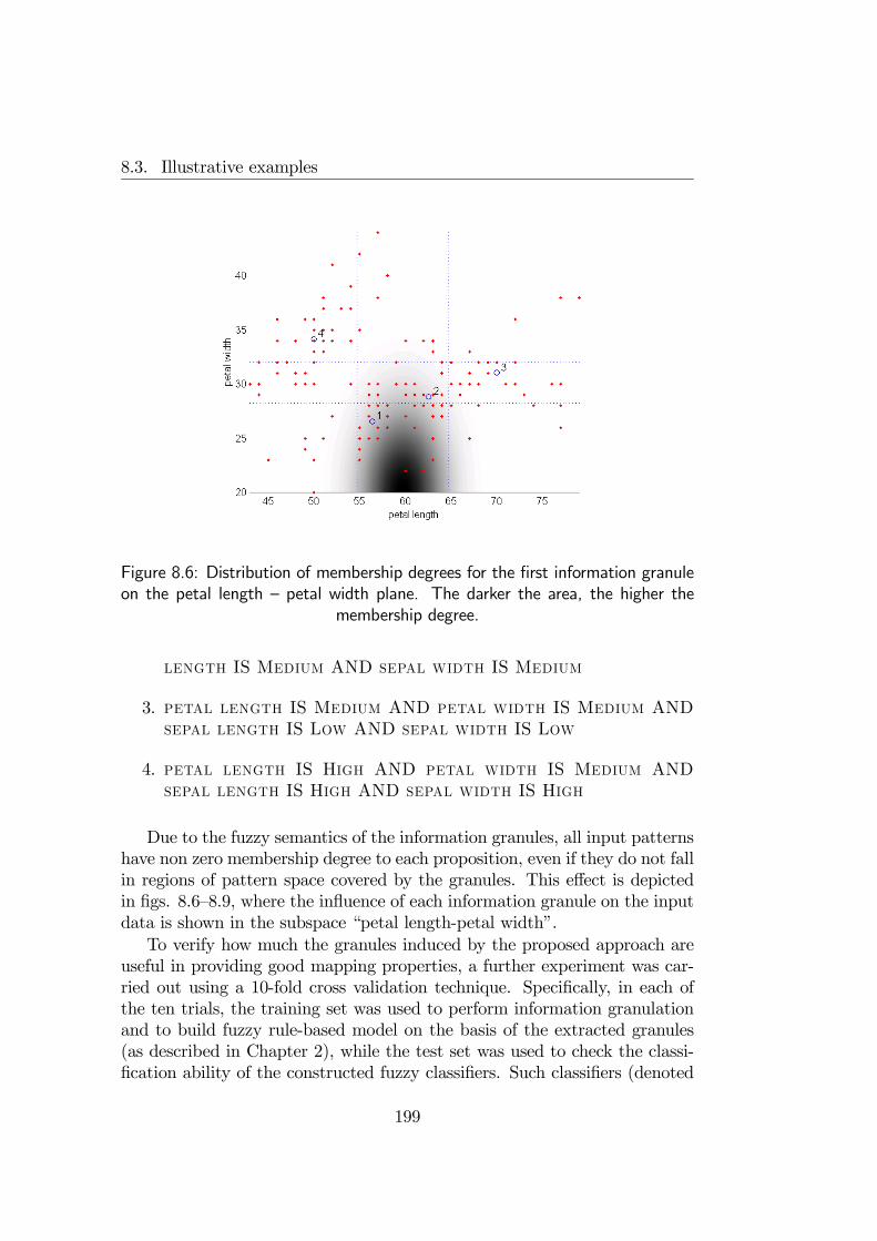
8.3. Illustrative examples
Figure 8.6: Distribution of membership degrees for the first information granuleon the petal length — petal width plane. The darker the area, the higher the
membership degree.
length IS Medium AND sepal width IS Medium
3. petal length IS Medium AND petal width IS Medium ANDsepal length IS Low AND sepal width IS Low
4. petal length IS High AND petal width IS Medium ANDsepal length IS High AND sepal width IS High
Due to the fuzzy semantics of the information granules, all input patternshave non zero membership degree to each proposition, even if they do not fallin regions of pattern space covered by the granules. This effect is depictedin figs. 8.6—8.9, where the influence of each information granule on the inputdata is shown in the subspace “petal length-petal width”.To verify how much the granules induced by the proposed approach are
useful in providing good mapping properties, a further experiment was car-ried out using a 10-fold cross validation technique. Specifically, in each ofthe ten trials, the training set was used to perform information granulationand to build fuzzy rule-based model on the basis of the extracted granules(as described in Chapter 2), while the test set was used to check the classi-fication ability of the constructed fuzzy classifiers. Such classifiers (denoted
199

Chapter 8. Information Granulation through Double Clustering
Figure 8.7: Distribution of membership degrees for the second information gran-ule on the petal length — petal width plane. The darker the area, the higher the
membership degree.
Figure 8.8: Distribution of membership degrees for the third information granuleon the petal length — petal width plane. The darker the area, the higher the
membership degree.
200
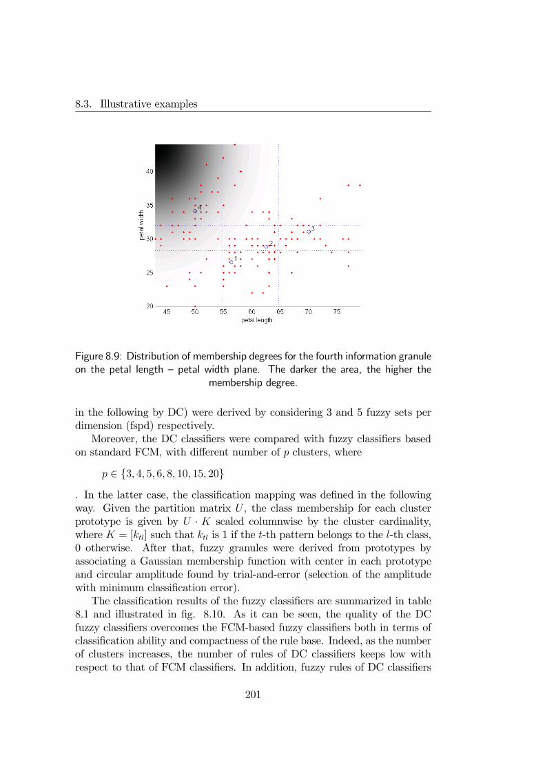
8.3. Illustrative examples
Figure 8.9: Distribution of membership degrees for the fourth information granuleon the petal length — petal width plane. The darker the area, the higher the
membership degree.
in the following by DC) were derived by considering 3 and 5 fuzzy sets perdimension (fspd) respectively.Moreover, the DC classifiers were compared with fuzzy classifiers based
on standard FCM, with different number of p clusters, where
p ∈ 3, 4, 5, 6, 8, 10, 15, 20. In the latter case, the classification mapping was defined in the followingway. Given the partition matrix U , the class membership for each clusterprototype is given by U · K scaled columnwise by the cluster cardinality,where K = [ktl] such that ktl is 1 if the t-th pattern belongs to the l-th class,0 otherwise. After that, fuzzy granules were derived from prototypes byassociating a Gaussian membership function with center in each prototypeand circular amplitude found by trial-and-error (selection of the amplitudewith minimum classification error).The classification results of the fuzzy classifiers are summarized in table
8.1 and illustrated in fig. 8.10. As it can be seen, the quality of the DCfuzzy classifiers overcomes the FCM-based fuzzy classifiers both in terms ofclassification ability and compactness of the rule base. Indeed, as the numberof clusters increases, the number of rules of DC classifiers keeps low withrespect to that of FCM classifiers. In addition, fuzzy rules of DC classifiers
201

Chapter 8. Information Granulation through Double Clustering
Table 8.1: Classification results of the fuzzy classifiers. Classification error isexpressed in terms of misclassification rate (%)
FCM DC 3 fspd DC 5 fspdTest Error Rul Test Error Rules Test Error Rules
p Mean Std es Mean Std Min Max Mean Std Min Max3 20.0 10.8 3 14.0 7.6 3 3 - - - -4 18.0 7.3 4 14.7 6.5 4 4 - - - -5 16.7 8.6 5 12.7 7.0 5 5 19.3 11.3 5 56 16.0 8.0 6 10.7 8.0 5 6 14.0 7.6 6 68 13.3 18.1 8 6.7 8.0 6 8 7.1 8.5 8 810 5.3 7.8 10 7.3 4.7 6 8 5.3 5.0 9 1015 5.3 4.0 15 4.0 3.3 8 10 4.7 3.1 12 1520 3.3 4.5 20 5.3 5.8 7 9 5.3 6.5 15 19
are nicely interpretable, as it can be seen in the following, where the rule baseof one of the DC fuzzy classifiers with 6 rules and 3 fuzzy sets per dimensionis described, and from fig. 8.11 in which the fuzzy sets on each dimensionare plotted.
1. if petal length is low and petal width is low and sepallength is medium and sepal width is medium then flower issetosa with degree 0.02, virginica with degree 0.86, versi-colour with degree 0.11
2. if petal length is low and petal width is medium and sepallength is low and sepal width is low then flower is setosawith degree 0.94, virginica with degree 0.05, versicolourwith degree 0.02
3. if petal length is low and petal width is high and sepallength is low and sepal width is low then flower is setosawith degree 0.94, virginica with degree 0.05, versicolourwith degree 0.02
4. if petal length is medium and petal width is high and sepallength is low and sepal width is medium then flower issetosa with degree 0.01, virginica with degree 0.63, versi-colour with degree 0.36
5. if petal length is medium and petal width is medium andsepal length is high and sepal width is high then flower is
202

8.3. Illustrative examples
Classification accuracy comparison
0.0%
5.0%
10.0%
15.0%
20.0%
25.0%
3 4 5 6 8 10 15 20number of clusters with FCM
Classificationerror
FCMDC (3 fspd)DC (5 fspd)
Figure 8.10: Comparison of the fuzzy classifiers in terms of classification error
Figure 8.11: Fuzzy sets used to define the rulebase for Iris classification
203

Chapter 8. Information Granulation through Double Clustering
setosa with degree 0.01, virginica with degree 0.17, versi-colour with degree 0.82
6. if petal length is high and petal width is medium and sepallength is high and sepal width is high then flower is setosawith degree 0.01, virginica with degree 0.11, versicolourwith degree 0.87
8.3.2 Fuzzy Diagnosis
To assess the effectiveness of the Double Clustering Framework in solvingreal-world problems, the well-known Wisconsin Breast Cancer (WBC) clas-sification problem has been considered. The original dataset consists of 699examples of breast cancer diagnosis. Each example is formed by ten at-tributes plus the class diagnosis (benign/malignant). Full details about thedataset can be found in (Blake and Merx, 1998).In order to effectively apply the proposed framework, the dataset has
been cleaned by removing one attribute (corresponding to the patient IDs)and all the examples with at least one missing value. The total number ofremoved examples is 16, hence the cardinality of the dataset used in the fuzzyinformation granulation process is 683.The dataset has been split according to the stratified 10-fold cross-val-
idation scheme. For each fold, the Double Clustering Framework has beenapplied, and the resulting multidimensional granules have been used to definefuzzy rules. Such rules have been employed to infer breast cancer diagnosisfor both the training set and the test set of the fold.Two implementations of the Double Clustering Framework have been
considered — namely the Crisp Double Clustering and DCClass — in order toobserve their different behavior in solving the same classification problem.For the Crisp Double Clustering, the simulation has been repeated withdifferent choices of both the number of multidimensional prototypes andthe number of fuzzy set for each dimension. In particular, the number ofprototypes ranges from 2 to 10, while the number of fuzzy sets per dimensionvaries from 2 to 4. In each trial, the coverage level ε is fixed to 0.5.In table 8.2, an example of fuzzy rule is reported. As it can be seen, read-
ability of the extracted rules is immediate. In figs. 8.12 and 8.13, the derivedone-dimensional fuzzy sets for two input features are illustrated. Moreover,classification results are reported in tables 8.3 and 8.4 for the training setand the test set respectively, by varying number of multidimensional proto-types and fuzzy sets per input (equal for each dimension). Each value is theaverage for all the 10 folds used in the simulation.
204

8.4. Final remarks
Table 8.2: An example of rule induced by the proposed methodIf
ClumpThickness is HIGH ANDUniformityOfCellSize is MED-LOW ANDUniformityOfCellSize is MED-LOW ANDMarginalAdhesion is MED-HIGH ANDSingleEpithelialCellSize is MED-LOW ANDBareNuclei is HIGH ANDBlandChromatin is MED-LOW ANDNormalNucleoli is MED-HIGH ANDMitoses is MED-LOW
Thencancer is BENIGN with degree 0.99171,MALIGN with degree 0.0082883.
The obtained results on the breast-cancer problem are comparable withthose obtained by other techniques proposed in literature (see, e.g. (Abonyiet al., 2002)), with the additional feature of that the derived rules are ex-pressed in a nicely human-interpretable way.
The same classification problem has been tackled through the appli-cation of DCClass. In this case, however, the number of fuzzy sets per inputis not specified as it is automatically defined within the granulation process.By fixing the number of multidimensional prototypes to six, the appli-
cation of DCClass provides ten rule sets with average classification error onthe test sets of 3.975%, while the mean number of rules is 3.6. When com-pared with similar approaches, like NEFCLASS (Nauck and Kruse, 1999),the achieved results confirm that the proposed tool is a valid technique toextract accurate knowledge from data.To assess the transparency of the resulting information granules, a rule set
of five rules has been chosen, which provides a classification error of 1.471%on the test set. The one-dimensional fuzzy sets derived from the applicationof DCClass satisfy the interpretability constraints defined in Section 8.1, asalso illustrated in figs. 8.14—8.16 for three input dimensions. For such fuzzysets, the association of meaningful linguistic label is straightforward.
8.4 Final remarks
In this Chapter, a framework for fuzzy information granulation has been pre-sented. Its key feature is the ability of generating information granules from
205
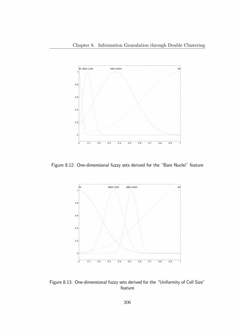
Chapter 8. Information Granulation through Double Clustering
0 0.1 0.2 0.3 0.4 0.5 0.6 0.7 0.8 0.9 1
0
0.2
0.4
0.6
0.8
1OW MED-LOW MED-HIGH HIG
Figure 8.12: One-dimensional fuzzy sets derived for the “Bare Nuclei” feature
0 0.1 0.2 0.3 0.4 0.5 0.6 0.7 0.8 0.9 1
0
0.2
0.4
0.6
0.8
1OW MED-LOW MED-HIGH HIG
Figure 8.13: One-dimensional fuzzy sets derived for the “Uniformity of Cell Size”feature
206
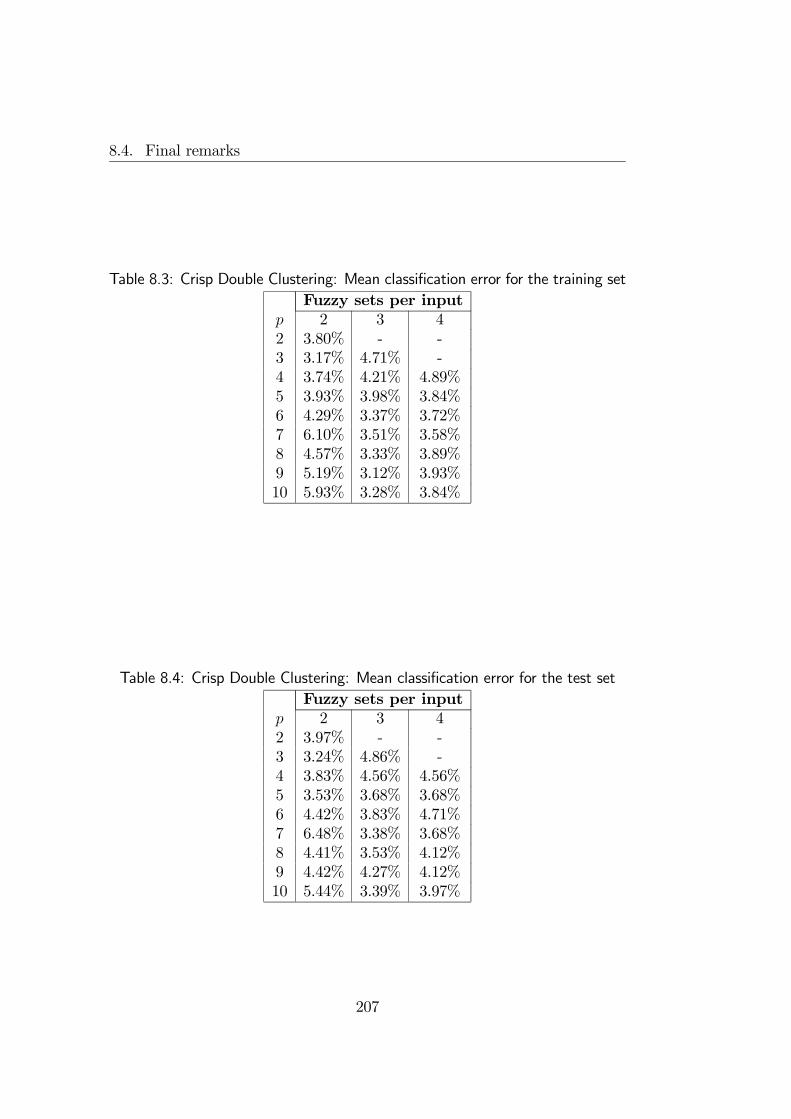
8.4. Final remarks
Table 8.3: Crisp Double Clustering: Mean classification error for the training setFuzzy sets per input
p 2 3 42 3.80% - -3 3.17% 4.71% -4 3.74% 4.21% 4.89%5 3.93% 3.98% 3.84%6 4.29% 3.37% 3.72%7 6.10% 3.51% 3.58%8 4.57% 3.33% 3.89%9 5.19% 3.12% 3.93%10 5.93% 3.28% 3.84%
Table 8.4: Crisp Double Clustering: Mean classification error for the test setFuzzy sets per input
p 2 3 42 3.97% - -3 3.24% 4.86% -4 3.83% 4.56% 4.56%5 3.53% 3.68% 3.68%6 4.42% 3.83% 4.71%7 6.48% 3.38% 3.68%8 4.41% 3.53% 4.12%9 4.42% 4.27% 4.12%10 5.44% 3.39% 3.97%
207
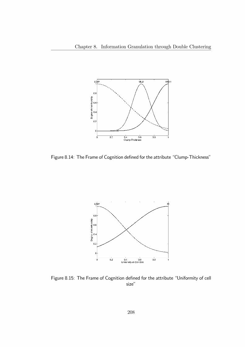
Chapter 8. Information Granulation through Double Clustering
Figure 8.14: The Frame of Cognition defined for the attribute “Clump-Thickness”
Figure 8.15: The Frame of Cognition defined for the attribute “Uniformity of cellsize”
208

8.4. Final remarks
Figure 8.16: The Frame of Cognition defined for the attribute “Uniformity of cellshape”
data which can be represented in terms of qualitative properties on data. Assupported by experimental examples, this feature turns very useful in all ap-plicative contexts — like fuzzy diagnosis — where an intelligible description of aphenomenon (like symptoms/diagnosis relationships) is of great importance.The framework is general enough to be extended with more sophisticated
techniques that may support a greater number of interpretability constraints,which could lead to the generation of knowledge structures that are morecomprehensible by human users.
209

Chapter 8. Information Granulation through Double Clustering
210
Chapter 9
Refinement of InterpretableInformation Granules throughNeural Learning
9.1 Introduction
Fuzzy information granules can be used as building blocks for designing fuzzymodels, often rule-based, which can be effectively employed to solve soft-computing problems such as predictions, classifications, system identification,etc. The added value of fuzzy models over “black-box” models (like neuralnetworks) is the explicit representation of the knowledge base in terms of sym-bolic structures, with the additional capability of handling vaguely definedconcepts by means of fuzzy sets. In this context, interpretable fuzzy infor-mation granulation plays an essential role in providing information granulesthat can be naturally associated to linguistic labels coming from the naturallanguage. As a result of such association, the knowledge base embodied intoa fuzzy model is easy to read and understand by human users.From a functional point of view, fuzzy models are approximative repre-
sentations of an underlying functional input/output relationship that has tobe discovered. To achieve such objective, often a dataset is available, whichprovides a finite collection of input/output examples from which the model’sknowledge has to be built. Information granulation techniques operate onsuch dataset to properly extract information granules that will be used todefine the model’s knowledge base. In this context, information granulationcan be accomplished in two main ways:
1. The complete dataset of examples is granulated, involving both inputand output information. At the end of the granulation process, the
211
Chapter 9. Refinement of Interpretable Information Granules throughNeural Learning
knowledge base of the fuzzy model is complete and can be immediatelyused for approximating the underlying functional relationship. A typ-ical example of fuzzy model defined by this kind of knowledge base isthe Mamdani Fuzzy Inference System;
2. The examples are split in the input and output components, and thegranulation process is executed only in the input part. This choice istypical in classification problems, where outputs are class labels thatbelong to a symbolic domain, which cannot be granulated. This formof granulation is also chosen when accuracy has a great impact in theassessment of the model quality.
When the second form of granulation is chosen, the resulting informationgranules are able to describe the relationships among input data, but theymiss to correctly represent the underlying input/output relationship. Whenoutput information is available, the knowledge base of the fuzzy model hasto be refined in order to better approximate the unknown functional rela-tionship, by means of supervised learning schemes1.The problem of model refinement through supervised learning has been
effectively solved by means of neuro-fuzzy networks. Neuro-fuzzy networksare translational architectures that map each element of the fuzzy modelinto an element of a suited neural network and vice-versa (Cloete and Zurada,2000). This bijective mapping allows for a dual view of the same system: as afuzzy model or as a neural network. In this way, learning techniques availablefor neural networks can be effectively applied to modify the parameters ofthe fuzzy model, whose knowledge base can thus be refined to accommodatethe underlying functional mapping.Neural learning schemes are very flexible and are able to adjust the net-
work parameters so as to finely approximate the unknown input/output rela-tionship described by the available dataset of examples. However, this strongflexibility may turn as a drawback in interpretable fuzzy modelling, since pa-rameters of the network — which are reflected into parameters of the model’sknowledge base and hence of the information granules — can easily change ina way that violates the interpretability constraints which guided the informa-tion granulation process. This drawback is particularly felt when informationgranules represent qualitative properties on data, since interpretability con-straints on such kind of granules are more stringent.
1It should be noted that information granulation on the input space can be consideredas an unsupervised learning scheme. The fuzzy model resulting from both unsupervisedand supervised learning is then a hybrid model.
212
9.1. Introduction
To protect interpretability of the model’s knowledge base, several ap-proaches have been proposed. Some of them apply a regularization term tothe learning objective, so as to penalize those configurations of parametersthat violate interpretability constraints (Jin et al., 1998a; Jin and Sendhoff,2003; Lozowski and Zurada, 2000; Valente de Oliveira, 1999b). Regular-ized learning is effective for interpretability constraints that can be partiallyviolated, and the violation degree must be represents as an explicit func-tion of the network parameters. This condition cannot be easily appliedto all interpretability constraints (e.g. leftmost/rightmost fuzzy sets, nat-ural zero positioning, etc.), thus regularized learning could be ineffectivein some cases. Furthermore, regularized learning procedures introduce newhyper-parameters whose automatic handling is difficult unless computation-ally complex mathematical techniques (Bengio, 2000; Craven and Wabba,1979) — or time-consuming trial-and-error strategies — are adopted.An alternative to regularized learning procedure is the adoption of genetic
algorithms, which provide for an evolutive process of network configurationsthat combine themselves and mutate in order to survive over a selectionprocess that promotes accurate and interpretable knowledge representations(Cordón et al., 2003; Marìn-Blàzquez and Shen, 2002; Riid et al., 2000; Her-rera et al., 1995; Ishibuchi and Yamamoto, 2002; Ishibuchi et al., 1997). Asan additional feature, the selection process can evaluate complex and multi-objective fitness functions that can represent interpretability constraints ofdifferent representations. The main disadvantage of genetic algorithms istheir computational cost, which could be too high to be acceptable in manyapplicative contexts.Other approaches have been proposed to cope with interpretable neural
learning, including the one described in (Altug et al., 1999; Chow et al., 1999)that make use of a classical back-propagation learning scheme integrated witha procedure that projects the actual configuration of parameters computedby back-propagation into another configuration of parameters that is closeto the actual but verifies a set of interpretability constraints. The projectionoperation is applied after each back-propagation iteration, resulting in highcomputational cost.To deal with computational cost of interpretable learning schemes, Nauck
and Kruse propose a family of fuzzy models, NEFCLASS, NEFCON andNEFPROX, which are translated in specific neural architectures that aretrained by means of heuristic learning rules to preserve interpretability whilesimultaneously adapting the knowledge base to data (Nauck et al., 1997).This approach is interesting for its low computational cost, but the introduc-tion of heuristic learning rules poses some serious questions concerning theirconvergence properties and optimality of the found solutions. Furthermore,
213
Chapter 9. Refinement of Interpretable Information Granules throughNeural Learning
good interpretation of the learning results cannot always be guaranteed, espe-cially for high-dimensional problems. Hence, in (Nauck and Kruse, 1999) theNEFCLASS algorithm is added with interactive strategies for pruning rulesand variables so as to improve readability. This approach provides goodresults, but it results in a long interactive process that cannot extract auto-matically rules from data but requires the ability of the user to supervisedand interpret the learning procedure in all its stages.The problem of interpretable learning from data can be theoretically ana-
lyzed by observing that the space of the network parameters actually containsa small subset of configuration referring to an interpretable knowledge. Themajor difficulty is hence to characterize this subset in such a way to providea specific neural architecture whose possible parameter configurations belongto this subspace only. Once this neural architecture is defined, classical learn-ing schemes can be safely applied, since the adaption process will entirely takeplace within the subspace of interpretable configurations. As a result, theknowledge base mapped in the neural network will be interpretable before,during and after the learning process. The rest of the Chapter is devoted indescribing this approach in a greater detail.
9.2 A neuro-fuzzy network to learn interpretableinformation granules
In this Section, a neuro-fuzzy architecture is proposed whose parameter spaceis restricted so that only interpretable fuzzy models are representable. First,such subspace (named “subspace of interpretable configurations”) is mathe-matically characterized. On the basis of such characterization, a neuro-fuzzyarchitecture is defined. Finally, a learning scheme based on the well-knowngradient-descent strategy is formalized and analyzed.
9.2.1 The subspace of interpretable configurations
To characterize the subspace of interpretable configurations, the followinginterpretability constraints are considered:
• Normality;• Convexity;• Unimodality;• Continuity;
214

9.2. A neuro-fuzzy network to learn interpretable information granules
• Weak proper ordering;
• Coverage (more specifically, ε-coverage for ε > 0);
• Distinguishability;
• Leftmost/Rightmost fuzzy sets.
It should be noted that such constraints are the same required for quali-tative information granulation. In this way, interpretable fuzzy informationgranules resulting from this form of granulation can be directly applied todesign fuzzy models which can be implemented according to the proposedarchitecture. The chosen characterization for distinguishability is by meansof the possibility function. For a simplified analysis, the maximum allowedpossibility in a Frame of Cognition is set to ε, i.e. the same threshold forcoverage. Furthermore, the value ε is assumed to be constant for each Frameof Cognition2.The aim of this Section is to characterize the subspace of interpretable
configurations independently from the specific information granulation tech-nique used to build the knowledge base. As a consequence, the simplestassumptions will be made on the knowledge base, which is characterized bya set of R rules of the form
Rule r :IF v1 is L³A(1)g(r,1)
´AND ... AND vn is L
³A(n)g(r,n)
´THEN <Consequent>
where L(A(i)g(r,i)) is the label associated to fuzzy set A(i)g(r,i) according tothe Frame of Cognition Fi of the i-th input feature. The consequent of therule is left unspecified since interpretability constraints do not apply to thispart of the rule. For convenience, the index specification of each fuzzy setis represented as a function g : 1, 2, . . . , R × 1, 2, . . . , n → N, so thatg (r, i) = k if in rule r the k-th fuzzy set of the Frame of Cognition i isused. The adoption of function g facilitates the representation of the rulebase within the neural architecture3.For the i-th input dimension, i = 1, 2, . . . , n, a Frame of Cognition con-
sisting of Ki fuzzy sets is defined and properly labelled. The definition ofsuch fuzzy sets, as well as the combinations of them occurring in the rules
2As will be clear forth, this is not a stringent requirement, which is set only for easiningthe discussion.
3Specifically, g (i, j) = k means that the k-th node of the j-th input in the MembershipLayer is connected to the i-th neuron of the Rule Layer
215
Chapter 9. Refinement of Interpretable Information Granules throughNeural Learning
antecedents is determined by the information granulation algorithm, like anyimplementation of the Double Clustering Framework.In most cases, fuzzy sets belonging to Frames of Cognition have a mem-
bership function with a fixed functional form, and one fuzzy set differ fromany other by the values of a set of parameters. As an example, Gaussianfuzzy set differ for their centers and amplitudes. As a consequence, the ar-ray of fuzzy sets occurring in a frame of cognition, properly sorted by therelated order relation of the frame, can be mapped bijectively into an arrayof parameters. For Gaussian fuzzy sets of center ω and width σ, a Frame ofCognition represented by fuzzy setsD
A(i)1 , A
(i)2 , . . . , A
(i)Ki
E(9.1)
is directly mapped into the vector that includes both centers and widths ofeach fuzzy set. The resulting parameter space can be defined as:
Ω(i) =
( ³ω(i)1 , ω
(i)2 , . . . , ω
(i)Ki, σ
(i)1 , σ
(i)2 , . . . , σ
(i)Ki
´∈ R2Ki :
∀h : mi ≤ ω(i)h < ω
(i)h+1 ≤Mi ∧ σ(i)i > 0
)(9.2)
where the order relation ω(i)h ≤ ω
(i)h+1 is given by the proper ordering of
fuzzy sets and by unimodality of Gaussian membership functions. It is alsoassumed that each fuzzy set of the Frame of Cognition is defined on theUniverse of Discourse Ui = [mi,Mi], as usual.Due to the independence of the elements of the parameter vector, the
dimensionality of each parameter space is 2Ki. The entire parameter spaceof the fuzzy model is defined as
Ω = Ω(1) × · · · × Ω(n) (9.3)
and has dimensionality
dimΩ = 2nXi=1
Ki (9.4)
Let
Ω∗ = Ω∗(1) × · · · ×Ω∗(n) (9.5)
be the subspace of interpretable configurations, i.e. the subspace of para-meters that correspond to fuzzy sets satisfying the aforementioned inter-pretability constraints. If Gaussian fuzzy sets are used, then the propertiesof normality, unimodality, continuity and convexity are satisfied for any value
216

9.2. A neuro-fuzzy network to learn interpretable information granules
assumed by centers and amplitudes. As a consequence, the constraints oncoverage and distinguishability — together with leftmost and rightmost con-straints — contribute in restricting the set of admissible values for centers andamplitudes.To characterize Ω∗ by means of formal conditions that enable the evalu-
ation of its dimensionality, the following lemma is particularly useful.
Lemma 9.1 For each pair of one-dimensional Gaussian membership func-tions (defined on the same Universe of Discourse) with centers and widthsω1, ω2 (such that ω1 < ω2) and σ1, σ2 respectively, there exists a unique pointt between their centers, for which the membership values are identical.Proof.The explicit representation of the Gaussian membership functions are:
µk (x) = exp
Ã−(x− ωk)
2
2σ2k
!, k = 1, 2 (9.6)
The intersection points of the two functions are:
T = t ∈ R : µ1 (t) = µ2 (t) (9.7)
By solving the equation characterizing the set T , the following point are obtained:
T =
nσ1ω2−σ2ω1
σ1−σ2 , σ1ω2+σ2ω1σ1+σ2
oif σ1 6= σ2n
σ2ω1+σ1ω2σ1+σ2
oif σ1 = σ2
(9.8)
In both cases, the point:
t =σ1ω2 + σ2ω1
σ1 + σ2(9.9)
is located between ω1 and ω2 since it is a convex combination of the two centers.If σ1 > σ2, then:
ω1 < ω2 =⇒ σ1ω2 − σ2ω1σ1 − σ2
> ω2 (9.10)
Conversely, if σ1 < σ2, then
ω1 < ω2 =⇒ σ1ω2 − σ2ω1σ1 − σ2
< ω1 (9.11)
In both cases, the point σ1ω2−σ2ω1σ1−σ2 is outside the range [ω1, ω2]; hence the point t
is unique.
If the fuzzy sets of a Frame of Cognition are constrained so as to sat-isfy ε-coverage and ε-possibility4, then the following proposition can be alsoasserted:
4With the term ε-possibility, it is intended that the maximum allowed possibility in aFrame of Cognition is ε.
217
Chapter 9. Refinement of Interpretable Information Granules throughNeural Learning
Proposition 9.1 LetDA(i)1 , A
(i)2 , . . . , A
(i)Ki
Ebe the family of ordered Gaussian
fuzzy set defined in a Frame of Cognition Fi. Suppose that the frame verifiesε-coverage and ε-possibility. Then, for any two adjacent fuzzy sets A(i)k , A
(i)k+1
there exists a unique intersection point tk such that µA(i)k(tk) = ε = µ
A(i)k+1(tk).
Proof.Consider the intersection point tk between two adjacent fuzzy sets A(i)k , A
(i)k+1
located between the two centers ω(i)k , ω(i)k+1. By virtue of the previous Lemma, such
point is unique. Three cases can be considered to analyze the value of µA(i)k
(tk). If,
ad absurdum, µA(i)k
(tk) > ε, then Π³A(i)k , A
(i)k+1
´> ε, but this is not possible since
ε-possibility is verified by hypotheses. Suppose, still ad absurdum, that µA(i)k
(tk) <
ε; by ε-coverage there would be a third fuzzy set A(i)h such that µA(i)h
(tk) ≥ ε
and h /∈ k, k + 1. Because of the proper ordering of the frame of cognition,the center ω
(i)h is not located between ω
(i)k and ω
(i)k+1. As a first case, consider
ω(i)h < ω
(i)k . In the interval
hω(i)h , th
hthe membership value of A(i)h is always greater
than ε and, in the unique intersection point t0hk between ω(i)h and ω(i)k there would be
µA(i)h
(t0hk) = µA(i)k
(t0hk) > ε, thus violating the ε-possibility constraint. Similarly,
if ω(i)h > ω(i)k+1 there would exist a point t
0hk+1 between ω
(i)h and ω
(i)k+1 such that
µA(i)h
¡t0hk+1
¢= µ
A(i)k+1
¡t0hk+1
¢> ε. This is absurd, hence the fuzzy set A(i)h cannot
exist and µA(i)k
(tk) cannot be less than ε. Since Gaussian membership functions
are continuos and have range ]0, 1], then it must be µA(i)k
(tk) = ε = µA(i)k+1
(tk).
As an important corollary of the proposition, the following theorem canbe stated:
Theorem 9.1 LetDA(i)1 , A
(i)2 , . . . , A
(i)Ki
Ebe the family of ordered Gaussian
fuzzy set defined in a Frame of Cognition Fi. Suppose that the frame ver-ifies ε-coverage and ε-possibility. The, there exists a unique vector t(i) =³t(i)1 , t
(i)2 , . . . , t
(i)Ki−1
´of intersection points between adjacent fuzzy sets of the
frame. Such intersection points verify the following inequalities:
mi < t(i)1 < t
(i)2 < . . . < t
(i)Ki−1 < Mi (9.12)
Proof.The existence and uniqueness of t(i) is a trivial consequence of Proposition9.1. The inequalities are also a direct consequence of the weak proper ordering ofthe fuzzy sets in the Frame of Cognition.
The last theorem is important because it reduces the vector of parametersof a Frame of Cognition into a vector of Ki − 1 intersection points between
218

9.2. A neuro-fuzzy network to learn interpretable information granules
adjacent fuzzy sets. By varying the parameters of the fuzzy sets in the frame,also the vector t(i) varies in a space that can be defined as:
T (i) =
( ³t(i)1 , t
(i)2 , . . . , t
(i)Ki−1
´∈ RKi−1 :
mi < t(i)1 < t
(i)2 < . . . < t
(i)Ki−1 < Mi
)(9.13)
An important question concerns the possibility of expanding a vector ofintersection points into a vector of parameters characterizing the member-ship functions of a Frame of Cognition. The following theorem affirmativelyanswers the question.
Theorem 9.2 Let
t(i) =³t(i)1 , t
(i)2 , . . . , t
(i)Ki−1
´∈ T (i) (9.14)
be a set of intersection points in [mi,Mi]. Then there exists a unique vector³ω(i)1 , ω
(i)2 , . . . , ω
(i)Ki, σ
(i)1 , σ
(i)2 , . . . , σ
(i)Ki
´∈ Ω∗(i) (9.15)
that corresponds to an ordered collection of Gaussian fuzzy setsDA(i)1 , A
(i)2 , . . . , A
(i)Ki
E(9.16)
with ε-coverage, ε-possibility and intersection point t(i)k between two adjacentfuzzy sets A(i)k , A
(i)k+1, for k = 1, 2, . . . ,Ki − 1.
Proof.Consider the following dummy points:
t(i)0 = 2mi − t
(i)1 (9.17)
and
t(i)Ki= 2Mi − t
(i)Ki−1 (9.18)
and consider the following values:
ω(i)k =
t(i)k−1 + t
(i)k
2(9.19)
and
σ(i)k =
t(i)k − t
(i)k−1
2√−2 ln ε (9.20)
219
Chapter 9. Refinement of Interpretable Information Granules throughNeural Learning
for k = 1, 2, . . . ,Ki. Since ∀k : t(i)k−1 < t(i)k < t
(i)k+1, then ω
(i)k < ω
(i)k+1 and σ
(i)k > 0,
hence the vector³ω(i)1 , ω
(i)2 , . . . , ω
(i)Ki, σ(i)1 , σ
(i)2 , . . . , σ
(i)Ki
´belongs to Ω(i). The unique
intersection point between the Gaussian fuzzy sets A(i)k , A(i)k+1 induced by parameters
ω(i)k , ω
(i)k+1 and σ
(i)k , σ
(i)k+1 is
t =σ(i)k ω
(i)k+1 + σ
(i)k+1ω
(i)k
σ(i)k + σ
(i)k+1
=
=
³t(i)k − t
(i)k−1
´³t(i)k + t
(i)k+1
´+³t(i)k+1 − t
(i)k
´³t(i)k−1 + t
(i)k
´2³t(i)k+1 + t
(i)k−1
´ =
=2t(i)k
³t(i)k+1 + t
(i)k−1
´2³t(i)k+1 + t
(i)k−1
´ = t(i)k (9.21)
The membership value at the intersection point is
µA(i)k
³t(i)k
´= exp
−³t(i)k − ω
(i)k
´22³σ(i)k
´2 = exp
−µt(i)k −
t(i)k−1+t
(i)k
2
¶22
µt(i)k −t
(i)k−1
2√−2 ln ε
¶2 = ε (9.22)
For x ∈hω(i)k , t
(i)k
ithen µ
A(i)k
(x) > ε because A(i)k is Gaussian. Similarly, for
x ∈ht(i)k , ω
(i)k+1
iresults µ
A(i)k+1
(x) > ε; hence ε-coverage is verified by the fuzzy sets
A(i)k and A
(i)k+1 in the interval
hω(i)k , ω
(i)k+1
i. Since:
Ki−1[k=1
hω(i)k , ω
(i)k+1
i= [mi,Mi] (9.23)
then ε-coverage is verified in the entire domain of the i-th feature. To verify ε-possibility, consider two adjacent fuzzy sets A(i)k , A
(i)k+1; for x < t
(i)k :
µA(i)k+1
(x) < µA(i)k
³t(i)k
´= ε =⇒ min
½µA(i)k+1
(x) , µA(i)k
(x)
¾< ε (9.24)
Similarly, for x > t(i)k :
µA(i)k
(x) < µA(i)k+1
³t(i)k
´= ε =⇒ min
½µA(i)k+1
(x) , µA(i)k
(x)
¾< ε (9.25)
As a consequence:
Π³A(i)k+1, A
(i)k
´= sup
x∈[mi,Mi]min
½µA(i)k+1
(x) , µA(i)k
(x)
¾= ε (9.26)
220
9.2. A neuro-fuzzy network to learn interpretable information granules
Thus ε-possibility is verified between A(i)k+1 and A
(i)k . Consider a third fuzzy set
A(i)h , and suppose h > k + 1; if Π
³A(i)k , A
(i)h
´> ε then the unique intersection
point t0hk between A(i)k and A
(i)h within
hω(i)k , ω
(i)h
iwould be greater than ε, as the
possibility value coincides with the membership value at the intersection point. As aconsequence, in the interval
ht0hk, ω
(i)h
ithe membership value of A(i)h is greater than
ε. If ω(i)h−1 ∈ht0hk, ω
(i)h
ithen the possibility Π
³A(i)h−1, A
(i)h
´would be greater than
ε, but this is absurd because it has been proved that the possibility of two adjacentfuzzy sets is always equal to ε. If ω(i)h−1 ∈
hω(i)k , t0hk
i, then Π
³A(i)k , A
(i)h−1
´> ε since
µA(i)k
(x) > ε for x ∈hω(i)k , t0hk
i. In this case, by performing a change of variable
h − 1 7−→ h it is possible to repeat the same considerations as above, which willlead to an absurdum or to another change of variables. In all cases, it is provedthat Π
³A(i)k , A
(i)h
´≤ ε for h > k + 1. In a similar manner, it can be proved that
Π³A(i)k , A
(i)h
´≤ ε for h < k.
The theorems 9.1 and 9.2 state that there is a bijective correspondencebetween the spaces Ω∗(i) and T (i). Since each space T (i) has a geometricdimensionality Ki − 1, then the dimensionality of the space of interpretableconfigurations is:
dimΩ∗ =nX
k=1
dimΩ(i)∗ =nX
k=1
(Ki − 1) (9.27)
Comparing (9.27) with (9.4), it is possible to affirm that:
dimΩ∗ < dimΩ (9.28)
that is, the number of free parameters necessary to generate interpretableconfigurations is smaller than the free parameters corresponding to the to-tality of centers and widths of all Gaussian fuzzy sets involved in the ruleantecedents.
9.2.2 The Neuro-Fuzzy architecture
Proofs of theorems 9.1 and 9.2 provide a constructive procedure to transformelements of the space T (i) in elements of spaces Ω∗(i) of interpretable config-urations of one-dimensional fuzzy sets. This procedure suggests a particularneuro-fuzzy architecture that is able to represent interpretable fuzzy rulesdefined by interpretable fuzzy information granules.The network architecture is depicted in fig 9.1. It is a feed-forward,
partially connected architecture defined by the following layers:
221

Chapter 9. Refinement of Interpretable Information Granules throughNeural Learning
Figure 9.1: The neuro-fuzzy architecture for learning interpretable rules.
Input Layer It simply spreads input vector x = (x1, x2, . . . , xn) to theMembership Layer, described forth.
T-Layer The nodes of such layer are grouped into blocks, where each blockcorresponds to an input feature. Each block is made up of Ki+1 linearSingle Input Single Output nodes, ordered from the left to the right.The first node is defined by the following transfer function:
oTi,0 = uTi,0 ·mi = mi (9.29)
being mi the infimum of the i-th feature range and the input uTi,0 is theinput signal, which is kept constantly to +1. The transfer function ofthe last node of the group is similarly defined as
oTi,Ki= uTi,Ki
·Mi =Mi (9.30)
being Mi the supremum of the i-th feature range and the input uTi,Ki
is constantly +1. These two nodes are not adjustable, i.e. they haveno free parameters. The remaining Ki − 1 nodes have a similar linearactivation function, defined as
oTi,k = uTi,k · ti,k = ti,k, k = 1, 2, . . . ,Ki − 1 (9.31)
222
9.2. A neuro-fuzzy network to learn interpretable information granules
Each of such nodes has one free parameter, ti,k, which is subject ofadaptation during learning. The input signal uTi,k is always fed to +1.Each group of the T-Layer represents an element of the subspace T (i).The constraint mi < ti,1 < · · · < ti,Ki < Mi must be guaranteed by theinitialization process as well as by the network learning process.
Membership Layer The nodes of this layer can are also grouped intoblocks, with each block corresponding to an input feature. The nodesof the layer provide for the calculation of the membership degrees foreach input feature, and are defined by three inputs and one output.The Membership Layer is connected both to the Input Layer and theT-Layer in a way that can be formalized by the definition of the inputsignals for each node:
uM,1i,k = oTi,k−1 (9.32)
uM,2i,k = xi (9.33)
uM,3i,k = oTi,k (9.34)
For k = 1, 2, . . . ,Ki. The transfer functions represent Gaussian mem-bership functions, with the centers and widths calculated by meansof outputs coming from the T-Layer. The definition of the transferfunctions are:
oMi,1 = exp
−³uM,2i,k − uM,1
i,k
´22³σ³2uM,1
i,k − uM,3i,k , uM,3
i,k
´´2
= exp
Ã− (xi −mi)
2
2 (σ (2mi − ti,1, ti,1))2
!= µ
A(i)1(xi) (9.35)
oMi,k = exp
−³uM,2i,k − ω
³uM,1i,k , uM,3
i,k
´´22³σ³uM,1i,k , uM,3
i,k
´´2 (9.36)
= exp
Ã−(xi − ω (ti,k−1, ti,k))
2
2 (σ (ti,k−1, ti,k))2
!= µ
A(i)k(xi) , (9.37)
k = 1, 2, . . . ,Ki (9.38)
223

Chapter 9. Refinement of Interpretable Information Granules throughNeural Learning
oMi,Ki= exp
−³uM,2i,Ki− uM,3
i,Ki
´22³σ³uM,1i,Ki
, 2uM,3i,Ki− uM,1
i,Ki,´´2
(9.39)
= exp
Ã− (xi −Mi)
2
2 (σ (ti,Ki , 2Mi − ti,Ki))2
!= µ
A(i)Ki
(xi) (9.40)
The distinguished definition of the extreme nodes vs. the middle nodesis necessary to satisfy the “leftmost/rightmost fuzzy sets” interpretabil-ity constraint. It is noteworthy that extreme nodes have no free para-meters, since centers and widths are determined by the two functionsω and σ defined as:
ω (t0, t00) =t0 + t00
2(9.41)
and
σ (t0, t00) =t00 − t0
2√−2 ln ε (9.42)
In this way, interpretability constraints are always guaranteed due tothe theoretical results shown in the previous Section.
Rule Layer This Layer combines fuzzy membership values coming from theMembership Layer to form the rule activation strengths. Each nodeshas n inputs and one output. The i-th input signal corresponds to oneoutput of the i-th block of the Membership Layer. The specific node ofsuch layer that is connected to a node of the Rule layer is determinedby the function g, which is in turn determined by the informationgranulation algorithm. The Rule Layer is composed of R nodes, onefor each rule, and the r-th node of the layer is characterized by thefollowing input signals:
uR,ir = oMi,g(r,i), i = 1, 2, . . . n (9.43)
The transfer function computes the rule activation strength, which isgenerally determined by a t-norm composition of the membership val-ues occurring in the rule antecedent. For the design of the neuro-fuzzyarchitecture, the product is chosen as a suitable t-norm because it iseverywhere differentiable. As a consequence, the transfer function isdefined as:
oRr =nYi=1
uR,ir =nYi=1
µA(i)g(r,i)
(xi) = µr (x) (9.44)
224
9.2. A neuro-fuzzy network to learn interpretable information granules
Again, the nodes of the Rule Layer have not free parameters, as theoutput signal is fully determined by the input signals.
Output Layer The role of such layer is to complete the inference process ofthe fuzzy model implemented by the neural network. For simplicity, a 0-order Takagi-Sugeno fuzzy model is chosen, though more sophisticatedmodels can be also considered. If the fuzzy model has m outputs, thenthere will be m nodes on the Output Layer. There are R input signalsfor each node, defined as:
uO,rj = oRr , r = 1, 2, . . . , R (9.45)
for j = 1, 2, . . . ,m. It can be noted that the definition of the inputsignal does not depend on the output index j, thus the Rule Layer andthe Output Layer are fully connected. The transfer function of eachnode reflects the inference rule of the fuzzy model:
oOj =
PRr=1 u
O,rj · vj,rPR
r=1 uO,rj
=
PRr=1 u
O,rj · vj,rPR
r=1 uO,rj
=
PRr=1 µr (x) · vj,rPR
r=1 µr (x)= yj (x)
(9.46)
Each node of the Output Layer has r free parameters vj,r which lin-early contribute to the determination of the final output. However,such parameters are not involved in the definition of interpretable con-figurations of the rules.
9.2.3 The Neuro-Fuzzy learning scheme
The learning process for the proposed neural model can be accomplishedin several ways, including hybrid ones that exploit the linear contributionsof the free parameters in the Output Layer. The simplest learning algo-rithm is, however, the back-propagation algorithm, which follows the gra-dient descent rule for updating the free parameters. Apart from simplicity,Back-propagation is able to update also the parameters of the T-Layer, thuscontributing to the refinement of the information granules codified in thenetwork.For the purpose of describing the learning algorithm, it is supposed that
a finite training set D of input/output pairs is available:
D =©x(1),d(1)
®,x(2),d(2)
®, . . . ,
x(N),d(N)
®ª(9.47)
225
Chapter 9. Refinement of Interpretable Information Granules throughNeural Learning
where x(p) =³x(p)1 , x
(p)2 , . . . , x
(p)n
´∈ X is an input pattern and d(p) =³
d(p)1 , d
(p)2 , . . . , d
(p)m
´∈ Rm is the corresponding desired output vector. The
objective of learning is to modify the free parameters of the neural networkso as to minimize an error function generally defined as
E =1
N
NXp=1
E¡S¡x(p)
¢,d(p)
¢(9.48)
where S : X → Rm is the functional mapping realized by the neural networkand E is a punctual error function that is averaged over all training patternsto obtain the final error value E.The error function E can have different formulations, depending on the
applicative context of the neuro-fuzzy model. For simplicity, it is temporarilyleft undefined. To derive the learning rule of the Back-propagation algorithm,the derivatives of the global error vale E with respect to any free parametermust be explicated. Let ξ be a generic free parameter (of any layer); thegeneral schema for the derivatives is:
∂E
∂ξ=1
N
NXp=1
∂E
∂ξ
¡S¡x(p)
¢,d(p)
¢(9.49)
which corresponds to:
∂E
∂ξ=1
N
NXp=1
·∂E
∂S
¡S,d(p)
¢ · ∂S∂ξ
¡x(p)
¢¸S=S(x(p))
(9.50)
In general, S is multidimensional, hence the product within the summationis a scalar product, which can be explicated as:
∂E
∂ξ=1
N
NXp=1
"mXj=1
∂E
∂yj
¡S,d(p)
¢ · ∂yj∂ξ
¡x(p)
¢#S=(y1,y2,...,ym)(x(p))
(9.51)
This general formulation decouples the derivatives of the Error Function,which depend only on the desired output d(p) and the actual output S, andthe derivatives that depend on the structure of the neural network. Thelatter depend on the specific free parameter ξ. If ξ ≡ vk,r, the derivativeformulation is:
∂yj∂vk,r
¡x(p)
¢=
∂
∂vk,r
PRr=1 µr
¡x(p)
¢ · vk,rPRr=1 µr (x
(p))= δjk
µr¡x(p)
¢PRr=1 µr (x
(p))(9.52)
226

9.2. A neuro-fuzzy network to learn interpretable information granules
where δjk is the Kronecker Symbol, δjk = 1 if j = k, otherwise δjk = 0. Thefollowing definition:
λ(p)r
¡x(p)
¢=
µr¡x(p)
¢PRr=1 µr (x
(p))(9.53)
will be useful in successive calculations.The derivatives of one output with respect to the center of a Gaussian
fuzzy set is
∂yj
∂ω(i)h
¡x(p)
¢=
RXs=1
∂yj∂µs
¡x(p)
¢ · ∂µs
∂ω(i)h
¡x(p)
¢(9.54)
where:
∂yj∂µs
¡x(p)
¢=
∂
∂µs
PRr=1 µr
¡x(p)
¢ · vj,rPRr=1 µr (x
(p))=
vj,s − yj¡x(p)
¢PRr=1 µr (x
(p))(9.55)
and:
∂µs
∂ω(i)h
¡x(p)
¢= δg(s,i),h · µs
¡x(p)
¢ · x(p)i − ω(i)h³
σ(i)h
´2 (9.56)
By combining (9.55) and (9.56) in (9.54), it results:
∂yj
∂ω(i)h
¡x(p)
¢=
x(p)i − ω
(i)h³
σ(i)h
´2 RXs=1
g(s,i)=h
¡vj,s − yj
¡x(p)
¢¢ · λ(p)s
¡x(p)
¢(9.57)
Similarly, the derivatives of one output with respect to the width of aGaussian fuzzy set can be derived:
∂yj
∂σ(i)h
¡x(p)
¢=
³x(p)i − ω
(i)h
´2³σ(i)h
´3 RXs=1
g(s,i)=h
¡vj,s − yj
¡x(p)
¢¢ · λ(p)s
¡x(p)
¢(9.58)
To complete the calculation, the derivatives with respect to the cut pointsmust be computed. From (9.19) and (9.20) it can be observed that the h-thcenter and width of i-th input feature depend on the (h− 1)-th and h-th cutpoint. As a consequence, the derivative of yj with respect to ti,h could bewritten as:
∂yj∂ti,h
=∂yj
∂ω(i)h
· ∂ω(i)h
∂ti,h+
∂yj
∂ω(i)h+1
· ∂ω(i)h+1
∂ti,h+
∂yj
∂σ(i)h
· ∂σ(i)h
∂ti,h+
∂yj
∂σ(i)h+1
· ∂σ(i)h+1
∂ti,h(9.59)
227

Chapter 9. Refinement of Interpretable Information Granules throughNeural Learning
for h = 1, 2, . . . ,Ki − 1 and i = 1, 2, . . . , n. Special cases must be consideredfor k = 1 and k = Ki − 1, since the relative cut points are associated toleftmost and rightmost fuzzy sets. For h = 2, 3, . . . ,Ki − 2 derivatives canbe explicated as:
∂ω(i)h
∂ti,h=1
2=
∂ω(i)h+1
∂ti,h(9.60)
and:
∂σ(i)h
∂ti,h= − 1
2√−2 ln ε = −
∂σ(i)h+1
∂ti,h(9.61)
Leftmost and rightmost derivatives are calculated as,
ω(i)1 = ω (2mi − ti,1, ti,1) = mi =⇒ ∂ω
(i)1
∂ti,1= 0 (9.62)
ω(i)Ki
= ω (tKi−1, 2Mi − tKi−1) =Mi =⇒∂ω
(i)Ki
∂ti,Ki−1= 0 (9.63)
and
σ(i)1 = σ (2mi − ti,1, ti,1) =
2ti,1 − 2mi
2√−2 ln ε =⇒ ∂σ
(i)1
∂ti,1=
1√−2 ln εσ(i)Ki= σ (tKi−1, 2Mi − tKi−1) =
2Mi − 2tKi−1
2√−2 ln ε
=⇒ ∂σ(i)Ki
∂ti,Ki−1= − 1√−2 ln ε (9.64)
To complete the computation of derivatives, the error function must nowbe taken into account. More specifically, the derivatives ∂E/∂yj must becomputed. If the neuro-fuzzy model is used for function approximation, themost appropriate error function is Mean Squared Error (MSE), defined as
EMSE (y,d) =mXj=1
(yj − dj)2 (9.65)
In such a case, the required derivatives are easily computed:
∂E
∂yj=
∂EMSE
∂yj= 2 (yj − dj) (9.66)
228

9.2. A neuro-fuzzy network to learn interpretable information granules
If the neuro-fuzzy model is used for classification tasks, other error func-tions can be used. As an example, the Approximate Differentiable EmpiricalRisk Functional (ADERF) proposed in (Castellano et al., 2004) could beadequate. The ADERF functional is defined as:
EADERF (y,d) =1
2
mXj=1
µµyjkykw
¶u
− dj
¶2(9.67)
where kykw is the Minkowski norm of order w. The derivative of such errorfunction has the following form:
∂E
∂yj=
∂EADERF
∂yj=
u
µyujkykuw
− dj
¶yu−1j
1− kyk−ww ywjkykww
+
− uyw−1j
kyku+ww
mXk=1k 6=j
µyukkykuw
− dk
¶yuk (9.68)
With all derivatives explicated, the gradient descent learning rule cancomputed. At any discrete instant τ and for any network parameter ξ, thelearning rule follows the law:
ξ [τ + 1] = ξ [τ ]− η [τ ]∂E
∂ξ[τ ] (9.69)
where η [τ ] is the learning rate. Variations of (9.69) can also be considered,e.g. to provide a lightweight learning procedure by taking into account onlyone pattern at time. Furthermore, derivatives formulations can be rearrangedso as to follow the Back-propagation update formulas.When the learning procedure is applied to train the neuro- fuzzy net-
work, an important question arises on the order of the elements of each T (i),as defined in (9.13). The respect of such constraint, which is fundamentalto guarantee understandability of fuzzy rules, depends on the value of thelearning rate. Indeed, if the learning rate is too high, the update formulas ofparameters ti,h could exchange the relative position of a couple ti,h and ti,h+1.If the exchange is not avoided, the updated configuration of network para-meters would not belong to T (i) anymore, thus resulting in non-interpretableconfigurations. On the other hand, if the learning rate is too small, conver-gence could be too slow to be acceptable. An important question arises onthe quantification of the upper bound allowed for the learning rate to avoiddangerous exchanges of parameter positions.
229
Chapter 9. Refinement of Interpretable Information Granules throughNeural Learning
In order to provide for such a quantification, for each discrete instantτ two consecutive cut points ti,h and ti,h+1 on a generic dimension i areconsidered. The following quantity is taken into account:
∆i,h [τ ] = ti,h+1 [τ ]− ti,h [τ ] (9.70)
By hypothesis, ∆i,h [0] > 0 since the the initial configuration of parame-ters is assumed to be in T (i). The sequence ∆i,h [0] ,∆i,h [1] , . . . ,∆i,h [τ ] , . . .is derived by the following relation:
∆i,h [τ + 1] = ti,h+1 [τ + 1]− ti,h [τ + 1] = (9.71)
= ti,h+1 [τ ]− η [τ ]∂E
∂ti,h+1[τ ]− ti,h [τ ] + η [τ ]
∂E
∂ti,h[τ ] =(9.72)
= ∆i,h [τ ] + η [τ ]
µ∂E
∂ti,h[τ ]− ∂E
∂ti,h+1[τ ]
¶(9.73)
It is noteworthy observing that:
∆i,h [τ + 1] < ∆i,h [τ ] ⇐⇒ ∂E
∂ti,h[τ ] <
∂E
∂ti,h+1[τ ] (9.74)
By assuming that ∆i,h [τ ] > 0 (i.e. non exchange between ti,h and ti,h+1 attime τ), exchange at time τ +1 is avoided if ∆i,h [τ + 1] ≥ ∆i,h [τ ]. However,if ∆i,h [τ + 1] < ∆i,h [τ ] then exchange can be still avoided if:
∆i,h [τ ]| z >0
+ η [τ ]|z>0
µ∂E
∂ti,h[τ ]− ∂E
∂ti,h+1[τ ]
¶| z
<0
> 0 (9.75)
that is:
0 < η [τ ] <∆i,h [τ ]
∂E∂ti,h+1
[τ ]− ∂E∂ti,h
[τ ](9.76)
Since the learning rate does not depend on the specific cut points consid-ered, nor on the specific input dimension, the upper bound for the learningrate is:
η [τ ] < minh,i
∆i,h [τ ]∂E
∂ti,h+1[τ ]− ∂E
∂ti,h[τ ]
(9.77)
Since∆i,h [τ ] by hypotheses, the upper bound of the learning rate is alwaysgreater than zero. As a consequence, relation (9.77) proves the existenceof a non-empty range of values admissible for learning rates. The exactcalculation of the upper bound is unnecessary, since a simple trial-and-errorprocedure can be adopted: if a learning rate causes the exchange of two cutpoints, then it is reduced (e.g. halved) and the update procedure is repeated.
230
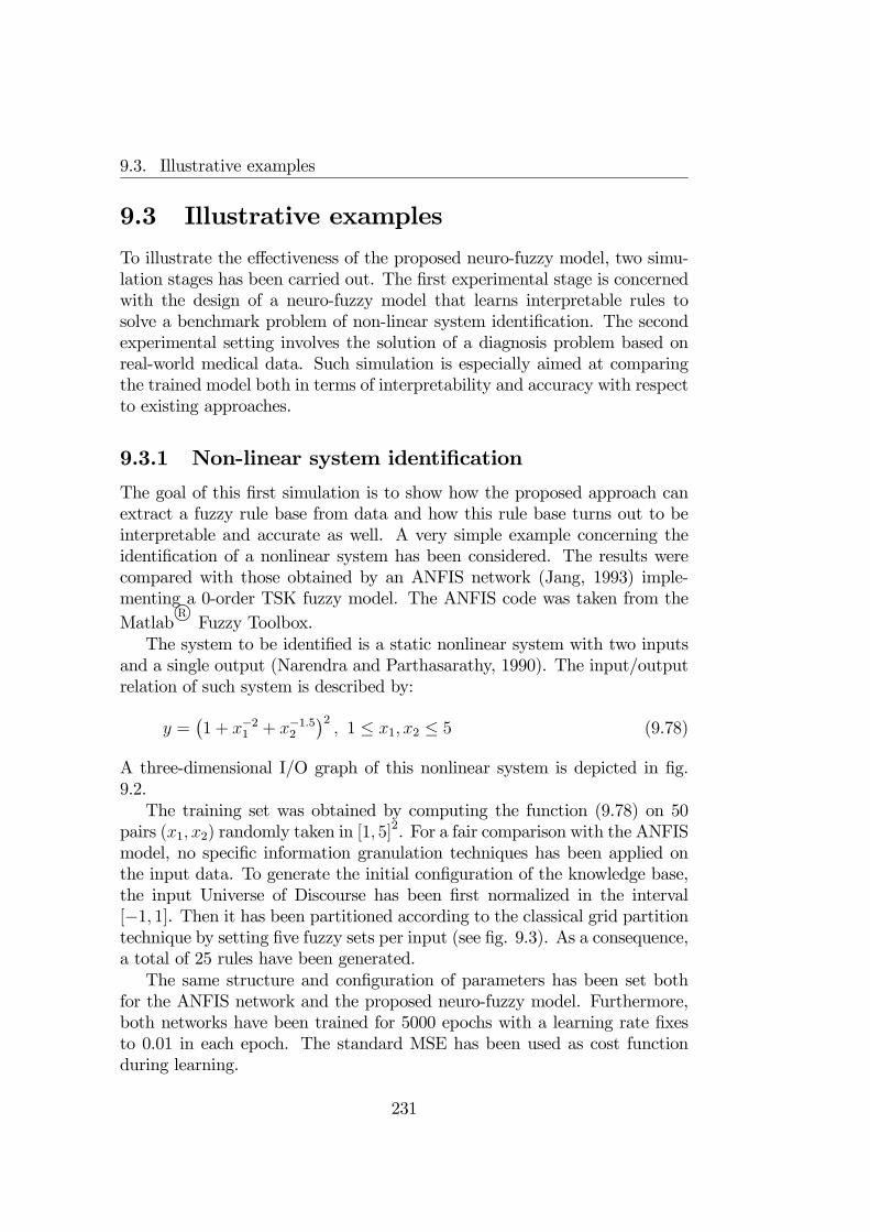
9.3. Illustrative examples
9.3 Illustrative examples
To illustrate the effectiveness of the proposed neuro-fuzzy model, two simu-lation stages has been carried out. The first experimental stage is concernedwith the design of a neuro-fuzzy model that learns interpretable rules tosolve a benchmark problem of non-linear system identification. The secondexperimental setting involves the solution of a diagnosis problem based onreal-world medical data. Such simulation is especially aimed at comparingthe trained model both in terms of interpretability and accuracy with respectto existing approaches.
9.3.1 Non-linear system identification
The goal of this first simulation is to show how the proposed approach canextract a fuzzy rule base from data and how this rule base turns out to beinterpretable and accurate as well. A very simple example concerning theidentification of a nonlinear system has been considered. The results werecompared with those obtained by an ANFIS network (Jang, 1993) imple-menting a 0-order TSK fuzzy model. The ANFIS code was taken from theMatlab
R°Fuzzy Toolbox.
The system to be identified is a static nonlinear system with two inputsand a single output (Narendra and Parthasarathy, 1990). The input/outputrelation of such system is described by:
y =¡1 + x−21 + x−1.52
¢2, 1 ≤ x1, x2 ≤ 5 (9.78)
A three-dimensional I/O graph of this nonlinear system is depicted in fig.9.2.The training set was obtained by computing the function (9.78) on 50
pairs (x1, x2) randomly taken in [1, 5]2. For a fair comparison with the ANFIS
model, no specific information granulation techniques has been applied onthe input data. To generate the initial configuration of the knowledge base,the input Universe of Discourse has been first normalized in the interval[−1, 1]. Then it has been partitioned according to the classical grid partitiontechnique by setting five fuzzy sets per input (see fig. 9.3). As a consequence,a total of 25 rules have been generated.The same structure and configuration of parameters has been set both
for the ANFIS network and the proposed neuro-fuzzy model. Furthermore,both networks have been trained for 5000 epochs with a learning rate fixesto 0.01 in each epoch. The standard MSE has been used as cost functionduring learning.
231
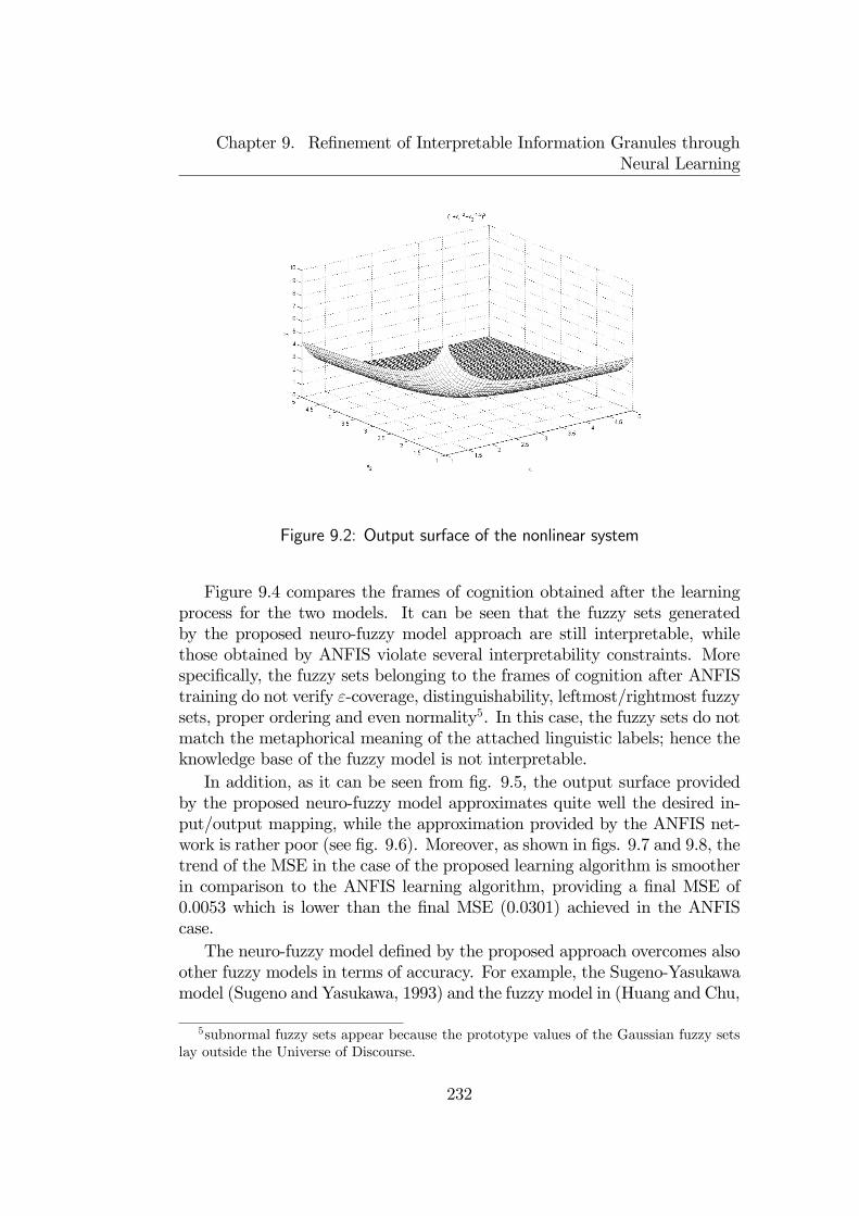
Chapter 9. Refinement of Interpretable Information Granules throughNeural Learning
Figure 9.2: Output surface of the nonlinear system
Figure 9.4 compares the frames of cognition obtained after the learningprocess for the two models. It can be seen that the fuzzy sets generatedby the proposed neuro-fuzzy model approach are still interpretable, whilethose obtained by ANFIS violate several interpretability constraints. Morespecifically, the fuzzy sets belonging to the frames of cognition after ANFIStraining do not verify ε-coverage, distinguishability, leftmost/rightmost fuzzysets, proper ordering and even normality5. In this case, the fuzzy sets do notmatch the metaphorical meaning of the attached linguistic labels; hence theknowledge base of the fuzzy model is not interpretable.In addition, as it can be seen from fig. 9.5, the output surface provided
by the proposed neuro-fuzzy model approximates quite well the desired in-put/output mapping, while the approximation provided by the ANFIS net-work is rather poor (see fig. 9.6). Moreover, as shown in figs. 9.7 and 9.8, thetrend of the MSE in the case of the proposed learning algorithm is smootherin comparison to the ANFIS learning algorithm, providing a final MSE of0.0053 which is lower than the final MSE (0.0301) achieved in the ANFIScase.The neuro-fuzzy model defined by the proposed approach overcomes also
other fuzzy models in terms of accuracy. For example, the Sugeno-Yasukawamodel (Sugeno and Yasukawa, 1993) and the fuzzy model in (Huang and Chu,
5subnormal fuzzy sets appear because the prototype values of the Gaussian fuzzy setslay outside the Universe of Discourse.
232
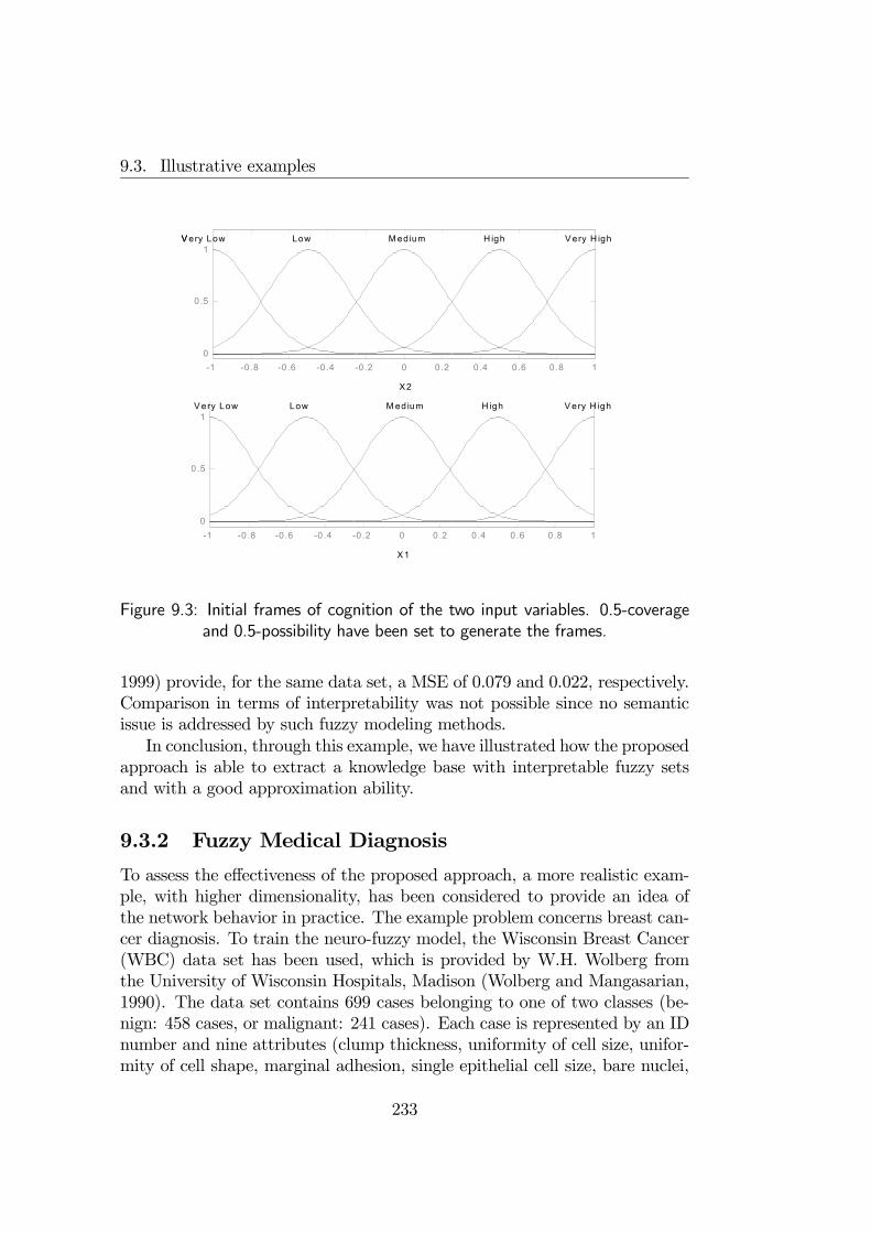
9.3. Illustrative examples
-1 -0 .8 -0.6 -0 .4 -0 .2 0 0.2 0.4 0 .6 0.8 10
0.5
1
X1
V ery Low Low M edium H igh V ery H igh
-1 -0 .8 -0 .6 -0 .4 -0 .2 0 0.2 0.4 0 .6 0.8 10
0.5
1
X2
V ery Low Low M edium H igh V ery H igh
-1 -0 .8 -0 .6 -0 .4 -0 .2 0 0 .2 0.4 0 .6 0.8 10
0.5
1
X 1
V ery Low Low M edium H igh V ery H igh
-1 -0 .8 -0 .6 -0 .4 -0 .2 0 0.2 0.4 0 .6 0.8 10
0.5
1
X2
V ery Low Low M edium H igh V ery H igh
Figure 9.3: Initial frames of cognition of the two input variables. 0.5-coverageand 0.5-possibility have been set to generate the frames.
1999) provide, for the same data set, a MSE of 0.079 and 0.022, respectively.Comparison in terms of interpretability was not possible since no semanticissue is addressed by such fuzzy modeling methods.In conclusion, through this example, we have illustrated how the proposed
approach is able to extract a knowledge base with interpretable fuzzy setsand with a good approximation ability.
9.3.2 Fuzzy Medical Diagnosis
To assess the effectiveness of the proposed approach, a more realistic exam-ple, with higher dimensionality, has been considered to provide an idea ofthe network behavior in practice. The example problem concerns breast can-cer diagnosis. To train the neuro-fuzzy model, the Wisconsin Breast Cancer(WBC) data set has been used, which is provided by W.H. Wolberg fromthe University of Wisconsin Hospitals, Madison (Wolberg and Mangasarian,1990). The data set contains 699 cases belonging to one of two classes (be-nign: 458 cases, or malignant: 241 cases). Each case is represented by an IDnumber and nine attributes (clump thickness, uniformity of cell size, unifor-mity of cell shape, marginal adhesion, single epithelial cell size, bare nuclei,
233
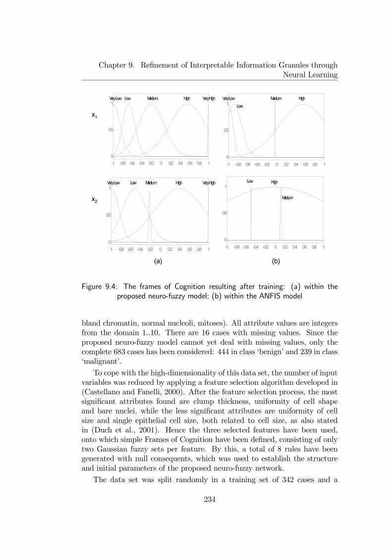
Chapter 9. Refinement of Interpretable Information Granules throughNeural Learning
-1 -0.8 -0.6 -0.4 -0.2 0 0.2 0.4 0.6 0.8 10
0.5
1 Very Low Low Medium High Very High
-1 -0.8 -0.6 -0.4 -0.2 0 0.2 0.4 0.6 0.8 1 0
0.5
1Low
Medium
High
-1 -0.8 -0.6 -0.4 -0.2 0 0.2 0.4 0.6 0.8 10
0.5
1 Very Low Low Medium High Very High
-1 -0.8 -0.6 -0.4 -0.2 0 0.2 0.4 0.6 0.8 10
0.5
1Very Low
Low
Medium High
x1
x2
(a) (b)
Figure 9.4: The frames of Cognition resulting after training: (a) within theproposed neuro-fuzzy model; (b) within the ANFIS model
bland chromatin, normal nucleoli, mitoses). All attribute values are integersfrom the domain 1..10. There are 16 cases with missing values. Since theproposed neuro-fuzzy model cannot yet deal with missing values, only thecomplete 683 cases has been considered: 444 in class ‘benign’ and 239 in class‘malignant’.
To cope with the high-dimensionality of this data set, the number of inputvariables was reduced by applying a feature selection algorithm developed in(Castellano and Fanelli, 2000). After the feature selection process, the mostsignificant attributes found are clump thickness, uniformity of cell shapeand bare nuclei, while the less significant attributes are uniformity of cellsize and single epithelial cell size, both related to cell size, as also statedin (Duch et al., 2001). Hence the three selected features have been used,onto which simple Frames of Cognition have been defined, consisting of onlytwo Gaussian fuzzy sets per feature. By this, a total of 8 rules have beengenerated with null consequents, which was used to establish the structureand initial parameters of the proposed neuro-fuzzy network.
The data set was split randomly in a training set of 342 cases and a
234

9.3. Illustrative examples
Figure 9.5: The input/output mapping realized by the proposed neuro-fuzzymodel
Figure 9.6: The input/output relationship realized by the ANFIS network
235
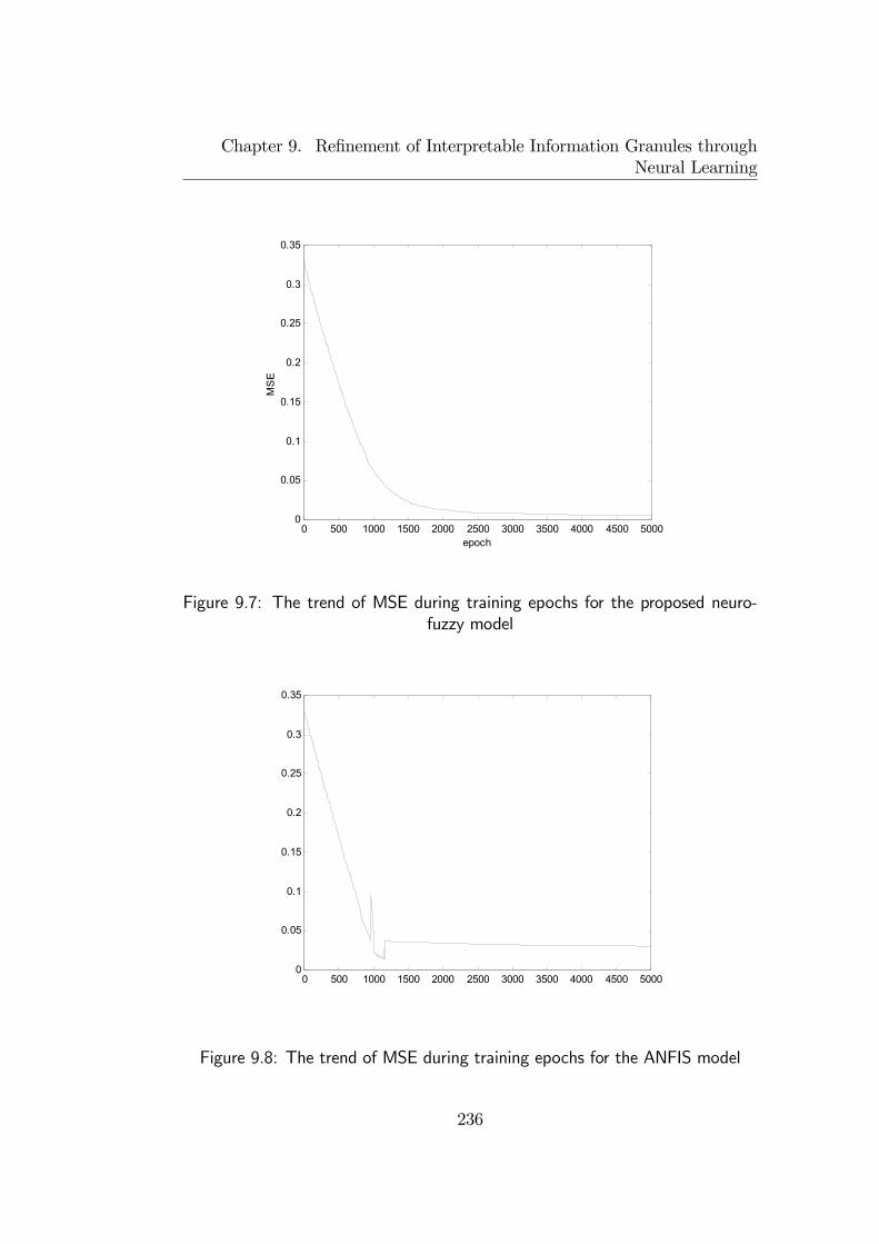
Chapter 9. Refinement of Interpretable Information Granules throughNeural Learning
0 500 1000 1500 2000 2500 3000 3500 4000 4500 50000
0.05
0.1
0.15
0.2
0.25
0.3
0.35
epoch
MS
E
Figure 9.7: The trend of MSE during training epochs for the proposed neuro-fuzzy model
0 500 1000 1500 2000 2500 3000 3500 4000 4500 50000
0.05
0.1
0.15
0.2
0.25
0.3
0.35
Figure 9.8: The trend of MSE during training epochs for the ANFIS model
236

9.3. Illustrative examples
1 2 3 4 5 6 7 8 9 100
0.1
0.2
0.3
0.4
0.5
0.6
0.7
0.8
0.9
1
clump thickness
Small Large
Figure 9.9: The refined frame of cognition for the feature “clump thickness”
test set of 341 cases, so that each set contains roughly the same number ofpatterns for each class. After 100 epochs of the proposed learning algorithm,a classification rate of 95.32% on the training set (16 errors), 96.48% on thetest set (12 errors), and 95.90% (28 errors) on the whole dataset has beenattained. For each variable, the two fuzzy sets (which have been labeled‘Small’ and ‘Large’) refined after learning are represented in figs. 9.9-9.11. The fuzzy sets and the frames of cognition verify all the requiredinterpretability constraints.Since in application areas like medicine interpretability is of great concern,
a small number of rules is highly desirable. As a consequence, the refinedknowledge base has been pruned according to the technique described in(Castellano and Fanelli, 1996), which automatically reduces the number ofrules while completely preserving the accuracy and the interpretability of theknowledge base. After rule simplification, there are only four fuzzy rules inthe rule base with unchanged fuzzy sets and accuracy with respect to the8-rule base. In the following, the discovered diagnostic rules are listed.
Rule 1: IF (clump thickness IS small) AND (uniformityof cell shape IS small) AND (bare nuclei IS small)THEN Patient belongs to class benign with degree0.67 and to class malignant with degree 0.11
Rule 2: IF (clump thickness IS small) AND (uniformityof cell shape IS small) AND (bare nuclei IS large)
237

Chapter 9. Refinement of Interpretable Information Granules throughNeural Learning
1 2 3 4 5 6 7 8 9 100
0.1
0.2
0.3
0.4
0.5
0.6
0.7
0.8
0.9
1
uniformity of cell shape
Small Large
Figure 9.10: The refined frame of cognition for the feature “uniformity of cellshape”
1 2 3 4 5 6 7 8 9 100
0.1
0.2
0.3
0.4
0.5
0.6
0.7
0.8
0.9
1
bare nuclei
Small Large
Figure 9.11: The refined frame of cognition for the feature “bare nuclei”
238

9.3. Illustrative examples
THEN Patient belongs to class benign with degree0.022 and to class malignant with degree 0.47
Rule 3: IF (clump thickness IS small) AND (uniformityof cell shape IS large) AND (bare nuclei IS small)THEN Patient belongs to class benign with degree0.00 and to class malignant with degree 0.54
Rule 4: IF (clump thickness IS large) AND (uniformityof cell shape IS small) AND (bare nuclei IS small)THEN Patient belongs to class benign with degree0.081 and to class malignant with degree 0.32
To evaluate the effectiveness of the resulting model in terms of accuracy,it has been compared with the NEFCLASS neuro-fuzzy system, also appliedto this dataset in (Nauck and Kruse, 1999), under the same experimentalsetting (i.e. removing 16 cases with missing values and partitioning the dataset into 342 samples for training and 341 for testing). Using 4 rules and“best-per-class” rule learning (which can be regarded as a kind of pruningstrategy), NEFCLASS achieves 8 errors on the training set (97.66% correct),18 errors on the test set (94.72% correct) and 26 errors (96.2% correct) on thewhole set. Despite the slightly better accuracy of NEFCLASS on the wholedataset, it should be noted that in case of the proposed neuro-fuzzy model,higher accuracy on the test set (generalization ability) is achieved with evena very small number of input variables with respect to the nine features usedby NEFCLASS, thus resulting in a more simple and interpretable rule base.Furthermore, it should be noted that results of the proposed model come fromthe application of automatic procedures, both for learning and simplification,that do not require human intervention unlike the NEFCLASS system.In addition, to obtain a more feasible estimate of the classification error, a
10-fold cross validation has been carried out. The data set was randomly splitinto ten equally sized parts without changing the class frequency. Each partwas used as test set for the knowledge base discovered from the remainingdata. The estimate of the classification accuracy was then computed asaverage of classification errors of all 10 neuro-fuzzy models on their test set.The mean error on the 10 test sets was 96.08% and the average number ofrules was 4.2 (ranging from 3 to 7 rules). A comparison with other neural,fuzzy and traditional classifiers developed for the same dataset is summarizedin table 9.1. It can be seen that the estimated classification of the proposedneuro-fuzzy model is comparable with most of the considered models. Indeed,most of the modeling methods reported in the table pursue only accuracy asultimate goal and take no care about the interpretability of the knowledgerepresentation.
239

Chapter 9. Refinement of Interpretable Information Granules throughNeural Learning
Table 9.1: Accuracy comparison of the proposed neuro-fuzzy model w.r.t. otherapproaches for the WBC dataset
Method Accuracy ReferenceIncNet 97.1% (1)
k-NN 97.0±0.12 (2)
Fisher LDA 96.8% (3)
MLP with Backprop 96.7% (3)
LVQ 96.6% (3)
Bayes (pairwise dep.) 96.6% (3)
Naïve Bayes 96.4% (3)
DB-CART 96.2% (4)
LDA 96.0% (3)
LFC,ASI,ASR 94.4%—95.6% (3)
CART 93.5% (4)
Quadratic DA 34.5% (3)
FSM, 12 rules 96.5% (2)
SSV, 3 rules 96.3%±0.2% (2)
NEFCLASS-X, 2 rules, 5-6 feat. 95.06% (5)
Proposed model 96.08%(1): (Jankowski and Kadirkamanathan, 1997)
(2): (Duch et al., 2001)
(3): (Ster and Dobnikar, 1996)
(4): (Shand and Breiman, 1996)
(5): (Nauck and Kruse, 1999)
240

9.4. Final remarks
9.4 Final remarks
In this Chapter, a neuro-fuzzy architecture and its learning algorithm forrefinement of fuzzy models with interpretability protection. Interpretabilityof fuzzy models is preserved during learning by allowing the free parametersto vary in a parameter subspace containing only configurations satisfying aset of formal properties.A simple benchmark and a real-world example have been considered to
illustrate the key features of the proposed model and its related learning al-gorithm. The given examples highlight that the proposed neural architecturecan be effective for model refinement, since the refined fuzzy models have anaccuracy comparable to other state-of-art models. Also, simulation resultsconfirm the essential feature of the proposed neuro-fuzzy architecture, thatis the ability to produce final rule bases that are also interpretable.Further extensions of the proposed model may concern the fulfillment
of additional interpretability requirements. As an example, the “UniformGranulation” interpretability constraint may be taken into account duringneural learning by checking the distance between consecutive cut points. Toembody such constraint, a threshold (or a penalization term) can be includedin the learning process so that such distances do not become too dissimilar.
241

Chapter 9. Refinement of Interpretable Information Granules throughNeural Learning
242

Part IV
Conclusions and FutureResearch
243


Conclusions and Future Research
The purpose of computing is insight,not numbers.(R. Hamming)
One of the fundamental motivations for the development of GranularComputing is to bring computer-based information processing closer to hu-man perception and reasoning. In this way it is hoped that complex problemscould be tackled and solved by computer systems following the well-knownprinciple postulated by Lotfi Zadeh:
[...] to exploit the tolerance for imprecision and uncertainty toachieve tractability, robustness, and low solution cost.
To cope with complex problems, the knowledge-oriented approach ap-pears the most successful, since it associates a general-purpose inferencemechanism with a problem-specific knowledge base that represents the prob-lem in a formal —hence machine treatable — way. The key feature of modelsbased on the Granular Computing paradigm is the organization of the knowl-edge base into chunks of information, the so-called information granules. Thisorganization has several advantages, like hierarchical decomposition, infor-mation hiding and user-centered modelling. Furthermore, the introductionof Fuzzy Logic into Granular Computing — which gives rise to the Theory ofFuzzy Information Granulation — enables the processing of vague knowledgethat highly pervades real-world problems.As a valuable consequence of modelling with the Theory of Fuzzy In-
formation Granulation, the knowledge base embodied in the model couldbe expressed in linguistic terms that are immediately intelligible by humanusers. However, interpretability of the knowledge base is not granted ipsofacto: fuzzy information granules must define a semantics that matches themetaphorical meaning conveyed by the associated linguistic representation.Interpretability within the Theory of Fuzzy Information Granulation raises
a number of issues that only recently have been taken into consideration. Theaim of this thesis has been to provide a number of contributions in this di-rection, both of theoretical and algorithmic type.The first issue taken under consideration in the thesis concerns the char-
acterization of interpretability in a mathematical fashion. A deep study ofexisting literature revealed that the constraint-based approach is the mosteffective for such a characterization, but there is not a general agreement ofwhich constraints mathematically define the blurry notion of interpretabilityin an exhaustive way. The first contribution of the thesis has hence been a
245
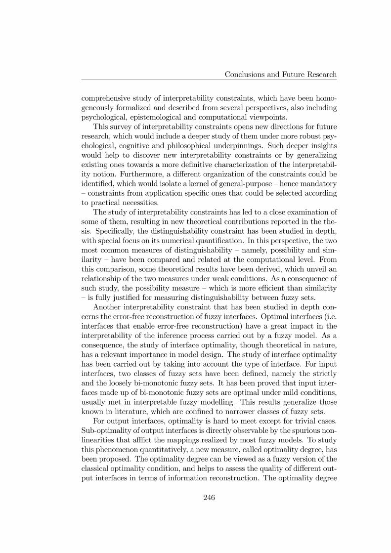
Conclusions and Future Research
comprehensive study of interpretability constraints, which have been homo-geneously formalized and described from several perspectives, also includingpsychological, epistemological and computational viewpoints.This survey of interpretability constraints opens new directions for future
research, which would include a deeper study of them under more robust psy-chological, cognitive and philosophical underpinnings. Such deeper insightswould help to discover new interpretability constraints or by generalizingexisting ones towards a more definitive characterization of the interpretabil-ity notion. Furthermore, a different organization of the constraints could beidentified, which would isolate a kernel of general-purpose — hence mandatory— constraints from application specific ones that could be selected accordingto practical necessities.The study of interpretability constraints has led to a close examination of
some of them, resulting in new theoretical contributions reported in the the-sis. Specifically, the distinguishability constraint has been studied in depth,with special focus on its numerical quantification. In this perspective, the twomost common measures of distinguishability — namely, possibility and sim-ilarity — have been compared and related at the computational level. Fromthis comparison, some theoretical results have been derived, which unveil anrelationship of the two measures under weak conditions. As a consequence ofsuch study, the possibility measure — which is more efficient than similarity— is fully justified for measuring distinguishability between fuzzy sets.Another interpretability constraint that has been studied in depth con-
cerns the error-free reconstruction of fuzzy interfaces. Optimal interfaces (i.e.interfaces that enable error-free reconstruction) have a great impact in theinterpretability of the inference process carried out by a fuzzy model. As aconsequence, the study of interface optimality, though theoretical in nature,has a relevant importance in model design. The study of interface optimalityhas been carried out by taking into account the type of interface. For inputinterfaces, two classes of fuzzy sets have been defined, namely the strictlyand the loosely bi-monotonic fuzzy sets. It has been proved that input inter-faces made up of bi-monotonic fuzzy sets are optimal under mild conditions,usually met in interpretable fuzzy modelling. This results generalize thoseknown in literature, which are confined to narrower classes of fuzzy sets.For output interfaces, optimality is hard to meet except for trivial cases.
Sub-optimality of output interfaces is directly observable by the spurious non-linearities that afflict the mappings realized by most fuzzy models. To studythis phenomenon quantitatively, a newmeasure, called optimality degree, hasbeen proposed. The optimality degree can be viewed as a fuzzy version of theclassical optimality condition, and helps to assess the quality of different out-put interfaces in terms of information reconstruction. The optimality degree
246
Conclusions and Future Research
could be viewed also as a starting point for newly devised output interfacesthat are specifically aimed at maximizing this measure. Such new outputinterfaces would drastically alleviate the problem of spurious nonlinearities,thus improving the interpretability of the inference process. The definitionand the implementation of such new interface is under investigation.Fuzzy information granules are often acquired from a set of available
observations. The process of fuzzy information granulation, which buildsinformation granules from data, must be tailored to verify interpretabilityconstraints, otherwise the resulting knowledge cannot be expressed with lin-guistic terms. This calls for brand new algorithms, or extension of existingones, for information granulation. Different algorithms can be devised onthe basis of the desired representation of the information granules, e.g. as aquantitative or as a qualitative description of data.A number of granulation algorithms have been proposed throughout this
work. For quantitative information granules, an algorithm for Gaussian in-formation granulation has been proposed, which can be used to wrap existingclustering algorithms (like Fuzzy C-Means) in order to derive interpretableinformation granules that can expressed as fuzzy numbers or fuzzy vectors.The granulation algorithm operates by solving a constrained quadratic op-timization problem based on the results of a fuzzy clustering algorithm. Itis shown that the solution of such optimization problem leads to compactinformation granules that can be effectively used to build accurate yet inter-pretable fuzzy models.For interval-valued information granules, a different approach has been
proposed. It extends the well-known Fuzzy C-Means clustering algorithm byprocessing Minkowski distances of any order on data. With the Minkowskiorder approaching infinity (in practice, for any order greater than about ten),this extended version of fuzzy clustering is able to discover boxlike-shapedclusters. The analysis of interference between clusters helps in choosing ap-propriate settings for the final definition of hyper-boxes, which could be de-composed as Cartesian product of intervals, either of crisp or of fuzzy type.The added value deriving from the adoption of intervals instead of scalar
values consists in the representation of an entire range of possibilities in-stead of a single quantity. This key feature has suggested the proposal ofextending the inference process of a fuzzy model to derive a prediction in-terval instead of a single numerical value. Prediction intervals, which havea sound meaning within the Theory of Probability, embody the knowledgeabout the uncertainty of the prediction carried out by a fuzzy model. Inthis way, the user can perceive the uncertainty of the model in providing thepredicted value. In this sense, the interpretability of the model is signifi-cantly improved. For such reason, prediction intervals have been adopted to
247

Conclusions and Future Research
extend a class of fuzzy models, and the added value of such approach hasbeen observed on a complex real-world problem.In some applicative contexts, a qualitative representation of information
granules is preferable. To generate interpretable information granules thatcan be described in terms of linguistic adjectives, like “small”, “cold”, etc.,an algorithmic framework has been proposed in this work. The framework,called “Double Clustering” is able to acquire from data information granulesthat verify a number of interpretability constraints so that they can be la-belled by linguistic adjectives of immediate semantics. The framework canbe implemented in several ways, according to applicative requirements. Fur-thermore, it is open to novel implementations that can further enhance thecapabilities of the framework. It is under investigation an implementation ofthe framework that makes use of a sophisticated informed search strategy,which could automatize the process of information granulation by selectingthe best granularity level in describing data so as to minimize the descriptionlength of the final representation.Fuzzy models design by means of information granulation processes could
be further refined if the internal knowledge is not completely defined by thederived information granules. When this occurs, a refinement process is nec-essary to complete the definition of the knowledge base. Neural learning is aneffective approach for this task, but without any control, the interpretabilityof the generated information granules can be seriously hampered. To copewith such a problem, a new neuro-fuzzy architecture has been proposed, to-gether with its learning scheme, which enable the refinement of the modelknowledge through neural learning without violating the interpretability con-straints for the tuned information granules. As a further enhancement, theproposed neuro-fuzzy network can be extended so as to satisfy a greaternumber of interpretability constraints, thus providing an even better inter-pretability of the resulting knowledge base.All the contributions presented in this work finally emerge as a unified
framework for interpretable information granulation and model design. Inthis direction, future developments will focus on the implementation of anextensible software tool that embodies all the proposed algorithms with pos-sibility of further extension to include newly devised algorithms. The toolwill allow the application of the proposed techniques for solving complexproblems coming from the real world. This could promote further investi-gations on interpretability issues within the Theory of Fuzzy InformationGranulation, both from theoretical and algorithmic standpoints.
248

List of Figures
1.1 Example of a granulation process . . . . . . . . . . . . . . . . 71.2 Basic epistemic relationships between labels, concepts and ob-
jects . . . . . . . . . . . . . . . . . . . . . . . . . . . . . . . . 14
2.1 Example of a nornal fuzzy set (solid) and a sub-normal fuzzyset (dashed) . . . . . . . . . . . . . . . . . . . . . . . . . . . . 25
2.2 A convex fuzzy set (solid) and a non-convex fuzzy set (dashed).While the convex fuzzy set may be associated to a semanti-cally sound lingusitic label, the non-convex fuzzy set conveysrepresents the semantic of a complex concept that is hard torepresent by a lingustic label. . . . . . . . . . . . . . . . . . . 27
2.3 An example of one-dimensional membership function that canbe derived by application of Fuzzy C-Means algorithm. . . . . 28
2.4 A Frame of Cognition with three fuzzy sets. While each in-dividual fuzzy sets has a well defined semantics, they are notproperly labelled thus hampering their interpretability . . . . 31
2.5 An example of violation of proper ordering . . . . . . . . . . . 332.6 Example of Frame of Cognition with a five fuzzy sets (a) and
another with ten fuzzy sets (b). The association of liguisticlabels to fuzzy sets of the first frame is clearly easier than tifuzzy sets of the second frame . . . . . . . . . . . . . . . . . . 35
2.7 Example of non-distinguishable fuzzy sets (dash vs. dash-dots) and distinguishable fuzzy sets (solid vs. dash or solidvs. dash-dots) . . . . . . . . . . . . . . . . . . . . . . . . . . . 36
2.8 Example of completeness violation. In the highlighted regionsof the Universe of Discourse (ellipses) 0.5-completeness is notverified. . . . . . . . . . . . . . . . . . . . . . . . . . . . . . . 38
2.9 Example of two frames of cognition with complementarity con-straint verified (a) and violated (b). . . . . . . . . . . . . . . . 43
2.10 Comparative example of two Frames of Congition where Uni-form Granulation is verified (a) and violated (b) . . . . . . . . 45
249

List of Figures
2.11 Example of a Frame of Cognition violating leftmost/rightmostfuzzy sets (a) and a frame veryfing such constraint (b). . . . . 47
2.12 Example of inference with rules in implicative interpretation.The inferred fuzzy set (bottom-right) is empty . . . . . . . . . 68
2.13 Example of inference with rules in conjuctive interpretation.The inferred fuzzy set (bottom right) represents two distinctand equally possible alternatives. . . . . . . . . . . . . . . . . 71
3.1 Example of fuzzy sets with full possibility but zero similarity . 923.2 Example of fuzzy set with low possibility . . . . . . . . . . . . 933.3 The contour of the min function (gray lines), the set Φ3 (shad-
owed) and an example of ΨA,B (dashed line) . . . . . . . . . . 973.4 The membership degree of intersection point between twomem-
bership functions corresponds to the possibility between thetwo fuzzy sets. . . . . . . . . . . . . . . . . . . . . . . . . . . 102
3.5 Example of fuzzy sets with maximal similarity for a given pos-sibility measure . . . . . . . . . . . . . . . . . . . . . . . . . . 103
3.6 Contour plot of maximal similarity Smax with respect to r andπ. . . . . . . . . . . . . . . . . . . . . . . . . . . . . . . . . . . 104
3.7 The cardinality of the intersection between A and B is thearea of the shaded region. . . . . . . . . . . . . . . . . . . . . 106
3.8 Functional relationship between possibility and similarity oftwo Gaussian fuzzy sets of equal width . . . . . . . . . . . . . 107
3.9 Two intersections between Gaussian fuzzy sets with differentwidth: (a) very different widths; (b) similar widths. . . . . . 108
4.1 The three functional blocks of a Fuzzy Model . . . . . . . . . 1164.2 Ambiguity areas in loosely bi-monotonic fuzzy sets . . . . . . 1234.3 The functional block diagram to calculate the optimality degree1264.4 Example of optimality degrees of two inferred outputs. The
value yoptimal has full optimality degree since its membershipdegrees w.r.t. output fuzzy sets coincide to those provided bytthe Processing Module for a given input x. In this sense, thevalue ysub-optimal has a very small optimality degree. . . . . . . 126
4.5 The membership functions of the input/output fuzzy sets forthe illustrative fuzzy model . . . . . . . . . . . . . . . . . . . 128
4.6 The behavior of the fuzzy model according to different choicesof defuzzification methods . . . . . . . . . . . . . . . . . . . . 129
4.7 Optimality Degrees for the illustrative fuzzy model accordingto different defuzzification procedures. . . . . . . . . . . . . . 130
250
List of Figures
5.1 The function (ξ − 1)2 (solid) is a second order approximationof log2 ξ (dashed) in the neighborhood of 1. . . . . . . . . . . 142
5.2 The North-East Dataset . . . . . . . . . . . . . . . . . . . . . 1445.3 Fuzzy granule for Philadelphia city and its Gaussian represen-
tation . . . . . . . . . . . . . . . . . . . . . . . . . . . . . . . 1455.4 Fuzzy granule for New York city and its Gaussian representation1465.5 Fuzzy Granule for Boston city and its Gaussian representation 1465.6 First granule representation . . . . . . . . . . . . . . . . . . . 1515.7 Second granule representation . . . . . . . . . . . . . . . . . . 1525.8 The Frame of Cognition for the “Weight” variable . . . . . . . 1525.9 The Frame of Cognition for the “Year” variable . . . . . . . . 153
6.1 Two distributions of membership degrees: (a) elliptical distri-bution; (b) boxed distribution. . . . . . . . . . . . . . . . . . 156
6.2 Shape of trapezoidal fuzzy set. The fuzzy set is well suited torepresent the fuzzy interval with core [b, c] . . . . . . . . . . . 163
6.3 Two-dimensional synthetic dataset with four visible clustersof unequal size . . . . . . . . . . . . . . . . . . . . . . . . . . . 164
6.4 Contour levels of a generated information granule, for p = 2 . 1656.5 Contour levels of a generated information granule, for p = 4 . 1666.6 Contour levels of a generated information granule, for p = 6 . 1666.7 Contour levels of a generated information granule, for p = 50 . 1676.8 Distortion evaluation for Minkowski distance in approximating
Tchebychev distance . . . . . . . . . . . . . . . . . . . . . . . 1676.9 The plot of φ1 vs. γ . . . . . . . . . . . . . . . . . . . . . . . . 1686.10 The plot of φ2 vs. γ . . . . . . . . . . . . . . . . . . . . . . . . 1696.11 The plot of φ3 vs. γ . . . . . . . . . . . . . . . . . . . . . . . . 1696.12 The plot of φ4 vs. γ . . . . . . . . . . . . . . . . . . . . . . . . 1706.13 Granular prototypes generated for p = 2 (dashed boxes) and
p = 50 (solid boxes) with φmax = 0.1 . . . . . . . . . . . . . . 170
7.1 The training dataset (circles) and the input/output mappingdefined by the neuro-fuzzy system (line) . . . . . . . . . . . . 178
7.2 Prediction intervals of the input/output mapping for four con-fidence levels (10%, 1%, 0.5%, 0.1%) . . . . . . . . . . . . . . 179
7.3 Estimation errors (solid line) and relative prediction intervals(dotted lines) for 8 models: Al (a), Ca (b), Mg (c), Ti (d), Ba(e), Co (f), V (g), Zi (h) . . . . . . . . . . . . . . . . . . . . . 182
8.1 The three steps of the Double Clustering Framework . . . . . 186
251
List of Figures
8.2 The first stage of DCClass. Data (dots and circles, accord-ing to the belonging class) are quantized into six prototypes,depicted as circles or squares depending on the associated class.196
8.3 The second stage of DCClass. Multidimensional prototypesare projected onto each dimension and then are clustered byaggregating prototypes belonging to the same class. . . . . . . 197
8.4 The third stage of DCClass. The clustered one-dimensionalprototypes determine the necessary information to generateone-dimensional Gaussian fuzzy sets. The multi-dimensionalprototypes enables the correct combination of such fuzzy setsto generate multidimensional information granules. . . . . . . 197
8.5 Result of the information granulation process plotted in twodimensions. The four cluster prototypes discovered by FuzzyC-means (circles) are projected on each axis and further clus-tered to produce three prototypes (diamonds) on each dimen-sion, resulting in three fuzzy sets per input variable. Dashedlines represent intersection points between adjacent fuzzy sets. 198
8.6 Distribution of membership degrees for the first informationgranule on the petal length — petal width plane. The darkerthe area, the higher the membership degree. . . . . . . . . . . 199
8.7 Distribution of membership degrees for the second informationgranule on the petal length — petal width plane. The darkerthe area, the higher the membership degree. . . . . . . . . . . 200
8.8 Distribution of membership degrees for the third informationgranule on the petal length — petal width plane. The darkerthe area, the higher the membership degree. . . . . . . . . . . 200
8.9 Distribution of membership degrees for the fourth informationgranule on the petal length — petal width plane. The darkerthe area, the higher the membership degree. . . . . . . . . . . 201
8.10 Comparison of the fuzzy classifiers in terms of classificationerror . . . . . . . . . . . . . . . . . . . . . . . . . . . . . . . . 203
8.11 Fuzzy sets used to define the rulebase for Iris classification . . 2038.12 One-dimensional fuzzy sets derived for the “Bare Nuclei” feature2068.13 One-dimensional fuzzy sets derived for the “Uniformity of Cell
Size” feature . . . . . . . . . . . . . . . . . . . . . . . . . . . . 2068.14 The Frame of Cognition defined for the attribute “Clump-
Thickness” . . . . . . . . . . . . . . . . . . . . . . . . . . . . . 2088.15 The Frame of Cognition defined for the attribute “Uniformity
of cell size” . . . . . . . . . . . . . . . . . . . . . . . . . . . . 2088.16 The Frame of Cognition defined for the attribute “Uniformity
of cell shape” . . . . . . . . . . . . . . . . . . . . . . . . . . . 209
252

List of Figures
9.1 The neuro-fuzzy architecture for learning interpretable rules. . 2229.2 Output surface of the nonlinear system . . . . . . . . . . . . . 2329.3 Initial frames of cognition of the two input variables. 0.5-
coverage and 0.5-possibility have been set to generate the frames.2339.4 The frames of Cognition resulting after training: (a) within
the proposed neuro-fuzzy model; (b) within the ANFIS model 2349.5 The input/output mapping realized by the proposed neuro-
fuzzy model . . . . . . . . . . . . . . . . . . . . . . . . . . . . 2359.6 The input/output relationship realized by the ANFIS network 2359.7 The trend of MSE during training epochs for the proposed
neuro-fuzzy model . . . . . . . . . . . . . . . . . . . . . . . . . 2369.8 The trend of MSE during training epochs for the ANFIS model2369.9 The refined frame of cognition for the feature “clump thickness”2379.10 The refined frame of cognition for the feature “uniformity of
cell shape” . . . . . . . . . . . . . . . . . . . . . . . . . . . . . 2389.11 The refined frame of cognition for the feature “bare nuclei” . . 238
253

List of Figures
254

List of Tables
3.1 Possibility and similarity measures for two common classes offuzzy sets (special cases not considered). . . . . . . . . . . . . 94
4.1 Some common defuzzification formulas . . . . . . . . . . . . . 1194.2 Comparison of Optimality Degree and Mean Squared Error
for a fuzzy model predicting the McKey Glass time series withdifferent defuzzification methods . . . . . . . . . . . . . . . . . 131
5.1 Parameters of the Gaussian Information Granules and MeanSquared Error . . . . . . . . . . . . . . . . . . . . . . . . . . . 145
5.2 Performace Measurements . . . . . . . . . . . . . . . . . . . . 1485.3 Average RMSE of the 10 Takagi-Sugeno models identified from
each fold. The total mean of RMSE is reported in the last row 1495.4 Comparison of the performance (RMSE) of Takagi-Sugeno
models with two input variables . . . . . . . . . . . . . . . . . 1505.5 Table of fufillment of interpretability constraints by Gaussian
Granulation (only applicable constraints are shown). . . . . . 154
6.1 Table of fufillment of interpretability constraints byMinkowskiGranulation (only applicable constraints are shown). . . . . . 172
7.1 Prediction errors with different confidence levels . . . . . . . . 1797.2 The ruleset generated for predicting Vanadium after the com-
bustion process, on the basis of the quantitis of Copper (Cu)and Vanadium (V) before combustion, and the drawing source.For ease of reading, the fuzzy sets in the rules antecedents havebeen represented by their respective 0.5-cuts . . . . . . . . . . 181
8.1 Classification results of the fuzzy classifiers. Classification er-ror is expressed in terms of misclassification rate (%) . . . . . 202
8.2 An example of rule induced by the proposed method . . . . . 205
255

List of Tables
8.3 Crisp Double Clustering: Mean classification error for thetraining set . . . . . . . . . . . . . . . . . . . . . . . . . . . . 207
8.4 Crisp Double Clustering: Mean classification error for the testset . . . . . . . . . . . . . . . . . . . . . . . . . . . . . . . . . 207
9.1 Accuracy comparison of the proposed neuro-fuzzy model w.r.t.other approaches for the WBC dataset . . . . . . . . . . . . . 240
256

Bibliography
Abonyi, J., Babuška, R., and Szeifert, F. (2002). Modified gath-geva fuzzyclustering for identification of takagi-sugeno fuzzy models. IEEE Transac-tions on Systems, Man and Cybernetics, part B, 32(5):612—621.
Abonyi, J., Roubos, H., Babuška, R., and Szeifert, F. (2003). Interpretablesemi-mechanistic fuzzy models by clustering, OLS and FIS model reduc-tion. In Casillas, J., Cordón, O., Herrera, F., and Magdalena, L., editors,Interpretability Issues in Fuzzy Modeling, pages 221—248. Springer-Verlag,Heidelberg.
Agarwal, L. and Taniru, M. (1992). A petri-net based approach for verifyingthe integrity of production systems. International Journal of man-machinestudies, 36:447—468.
Altug, S., Chow, M.-Y., and Trussel, H. J. (1999). Heuristic constraintsenforcement for training of and rule extraction from a Fuzzy/Neural archi-tecture — part II: Implementation and application. IEEE Transactions onFuzzy Systems, 7(2):151—159.
Angelov, P. (2004). An approach for fuzzy rule-base adaptation using on-lineclustering. International Journal of Approximate Reasoning, 35:275—289.
Auephanwiriyakul, S. and Keller, J. (2002). Analysis and efficient implemen-tation of a linguistic fuzzy c-means. IEEE Transactions on Fuzzy Systems,10(5):563—582.
Babuška, R. (1998). Fuzzy Modeling and Control. Kluwer, Norwell, MA.
Babuška, R. (1999). Data-driven fuzzy modeling: Transparency and com-plexity issues. In Proceedings 2nd European Symposium on Intelligent Tech-niques ESIT’99, Crete, Greece. ERUDIT.
Baraldi, A. and Blonda, P. (1999). A survey on fuzzy clustering algorithmsfor pattern recognition I/II. IEEE Transactions on Systems, Man and Cy-bernetics, part B, 29(6):778—801.
257
Bibliography
Baranyi, P., Yam, Y., Tikk, D., and Patton, R. (2003). Trade-off betweenapproximation accuracy and complexity: TS controller design via HOSVDbased complexity minimization. In Casillas, J., Cordón, O., Herrera, F.,and Magdalena, L., editors, Interpretability Issues in Fuzzy Modeling, pages249—277. Springer-Verlag, Heidelberg.
Bargiela, A. (2001). Interval and ellispoidal uncertainty in water systemstate estimation. In Pedrycz, W., editor, Granular Computing: An Intro-duction, pages 23—57. Physica-Verlag.
Bargiela, A. and Pedrycz, W. (2003a). Granular Computing: An Introduc-tion. Kluwer Academic Publishers, Boston, Dordrecht, London.
Bargiela, A. and Pedrycz, W. (2003b). A model of granular data: A designproblem with the tchebyschev fuzzy c-means. Soft Computing, (online first).
Barsalou, L. (1999). Perceptual symbol systems. Behavioral and BrainSciences, 22:577—660.
Bellman, R. (1961). Adaptive Control Processes: A Guided Tour. PrincetonUniversity Press, Princeton, NJ.
Bellman, R. and Giertz, M. (1973). On the analytic formalism of the theoryof fuzzy sets. Information sciences, 5:149—156.
Bellman, R., Kalaba, L., and Zadeh, L. (1966). Abstraction and patternclassification. Journal of Mathematical Analysis and Applications, 13:1—7.
Bengio, Y. (2000). Gradient-based optimization of hyper-parameters.Neural Computation, 12(8).
Berenji, H. and Khedkar, P. (1993). Clustering in product space for fuzzyinference. In Proceedings of the Second IEEE International Conference onFuzzy Systems, pages 1402—1407, San Francisco. IEEE.
Bettini, C. and Montanari, A., editors (2000). Spatial and Temporal Gran-ularity: Papers from the AAAI Workshop. The AAAI Press, Menlo Park,CA.
Bettini, C. and Montanari, A. (2002). Research issues and trends in spatialand temporal granularities. Annals of Mathematics and Artificial Intelli-gence, 36:1—4.
Bezdek, J. (1981). Pattern Recognition with Fuzzy Objective Function Al-gorithms. Plenum, New York.
258
Bibliography
Bezdek, J. (1992). On the relationship between neural networks, patternrecognition and intelligence. Journal of Approximate Reasoning, 6:85—107.
Bikdash, M. (1999). A highly interpretable form of sugeno inference systems.IEEE Transactions on Fuzzy Systems, 7(6):686—696.
Bishop, C. (1995). Neural Networks for Pattern Recognition. Oxford Uni-versity Press, Oxford, UK.
Blake, C. and Merx, C. (1998). UCI repository of machine learning data-bases. http://www.ics.uci.edu/ mlearn/MLRepository.html.
Bonarini, A. (1997). Anytime learning and adaptation of hierarchical fuzzylogic behaviors. Adaptive Behavior Journal, Special Issue on CompleteAgent Learning in Complex Environments, 5(3-4):281—315.
Butz, C. and Lingras, P. (2004). Granular jointree probability propaga-tion. In Proceedings of the 2004 Conference of the North American FuzzyInformation Processing Society (NAFIPS’04), pages 69—72, Banff, Alberta.
Casillas, J., Cordón, O., Herrera, F., and Magdalena, L., editors (2003).Interpretability Issues in Fuzzy Modeling. Springer, Germany.
Castellano, G., Castiello, C., Fanelli, A., and Giovannini, M. (2003a). Aneuro-fuzzy framework for predicting ash propeties in combustion processes.Neural, Parallel and Scientific Computation, 11:69—82.
Castellano, G., Castiello, C., Fanelli, A., and Mencar, C. (2003b). Discov-ering prediction rules by a neuro-fuzzy modeling framework. In Palade, V.,Howlett, R., and Jain, L., editors, Knowledge-Based Intelligent Informationand Engineering Systems (KES 2003), volume I, pages 1242—1248. Springer.
Castellano, G. and Fanelli, A. (1996). Simplifying a neuro-fuzzy model.Neural Processing Letters, 4(6):75—81.
Castellano, G. and Fanelli, A. (2000). Variable selection using neural net-work models. Neurocomputing, 31(14):1—13.
Castellano, G., Fanelli, A., and Mencar, C. (2001). Automatic fuzzy en-coding of complex objects. In Proceedings of the Joint 9th IFSA WorldCongress and 20th NAFIPS International Conference, pages 407—410.
Castellano, G., Fanelli, A., and Mencar, C. (2004). An empirical risk func-tional to improve learning in a neuro-fuzzy classifier. IEEE Transactions onSystems, Man and Cybernetics, part B, 34(1):725—731.
259
Bibliography
Castellano, G., Fanelli, A. M., and Mencar, C. (2002). A neuro-fuzzynetwork to generate human understandable knowledge from data. Cogni-tive Systems Research, Special Issue on Computational Cognitive Modeling,3(2):125—144.
Chepoi, V. and Dumitrescu, D. (1999). Fuzzy clustering with structuralconstraints. Fuzzy Sets and Systems, 105:91—97.
Chiang, J.-H., Yue, S., and Yin, Z.-X. (2004). A new fuzzy cover approachto clustering. IEEE Transactions on Fuzzy Systems, 12(2):199—208.
Chow, M.-Y., Altug, S., and Trussel, H. J. (1999). Heuristic constraintsenforcement for training of and knowledge extraction froma Fuzzy/Neuralarchitecture—part i: Foundation. IEEE Transactions on Fuzzy Systems,7(2):143—150.
Cios, K., Pedrycz, W., and Swiniarski, R. (1998). Data Mining. Methodsfor Knowledge Discovery. Kluwer.
Cloete, I. and Zurada, J., editors (2000). Knowledge-Based NeuroComput-ing. MIT Press.
Combs, W. E. and Andrews, J. E. (1998). Combinatorial rule explosioneliminated by a fuzzy rule configuration. IEEE Transactions on Fuzzy Sys-tems, 6(1):1—11.
Cordón, O., Del Jesus, M., Herrera, F., Magdalena, L., and Villar, P. (2003).A multiobjective genetic learning process for joint feature selection andgranularity and context learning in fuzzy rule-based classification systems.In Casillas, J., Cordón, O., Herrera, F., and Magdalena, L., editors, Inter-pretability Issues in Fuzzy Modeling, pages 79—99. Springer-Verlag, Heidel-berg.
Cordón, O. and Herrera, F. (2000). A proposal for improving the accuracyof linguistic modeling. IEEE Transactions on Fuzzy Systems, 8(3):335—344.
Corsini, P., Lazzerini, B., and Marcelloni, F. (2004). A fuzzy relationalclustering algorithm based on a dissimilarity measure extracted from data.IEEE Transactions on Systems, Man and Cybernetics, part B, 34(1):775—781.
Craven, P. and Wabba, G. (1979). Smoothing noisy data with spline func-tions: Estimating the correct degree of smoothing by the method of gener-alized cross-validation. Numerische Mathematik, 31:377—403.
260

Bibliography
Cressie, N. (1993). Statistics for Spatial Data. Wiley.
Cross, V. (1993). An analysis of fuzzy set aggregators and compatibilitymeasures. Master’s thesis, Dept. of Electronic Engineering, University ofDelft.
Czogala, E. and Leski, J. (2000). Fuzzy and Neuro-Fuzzy Intelligent Systems.Physica-Verlag, Heidelberg, Berlin.
de Oliveira, J. (1993). On optimal fuzzy systems I/O interfaces. In Pro-ceedings of the 2nd IEEE International Conference on Fuzzy Systems, pages851—865, San Francisco, CA.
de Oliveira, J. (1995). A set-theoretical defuzzification method. Fuzzy Setsand Systems, 76:63—71.
de Oliveira, J. (1996). Sampling, fuzzy discretization, and signal reconstruc-tion. Fuzzy Sets and Systems, 79:151—161.
Dempster, A. (1966). New methods for reasoning toward posterior distribu-tions based on sample data. Annals of Mathematical Statistics, 37:355—374.
Dick, S. and Kandel, A. (1999). Comment on "combinatorial rule explo-sion eliminated by a fuzzy rule configuration" (with author’s reply). IEEETransactions on Fuzzy Systems, 7(4):475—478.
Dreyfus, H. and Dreyfus, S. (1986). Mind over Machine: The Power ofHuman Intuition and Expertise in the Era of the Computer. MIT Press,Cambridge, MA.
Dubois, D. and Prade, H. (1980). Fuzzy Sets and Systems: Theory andApplications. Academic Press, New York.
Dubois, D. and Prade, H. (1988). Possibility Theory: An Approach toComputerized Processing of Uncertainty. Plenum Press, New York.
Dubois, D. and Prade, H. (1992). Evidence, knowledge and belief functions.International Journal of Approximate Reasoning, 6:295—319.
Dubois, D. and Prade, H. (1996). What are fuzzy rules and how to usethem. Fuzzy Sets and Systems, 84:169—185.
Dubois, D. and Prade, H. (1997). The three semantics of fuzzy sets. FuzzySets and Systems, 90:141—150.
261
Bibliography
Duch, W., Adamczak, R., and Grabczewski, K. (2001). A new methodologyof extraction, optimization and application of crisp and fuzzy logical rules.IEEE Transactions on Neural Networks, 12(2):277—306.
Dybowski, R. and Roberts, S. (2001). Confidence intervals and predictionintervals for feed-forward neural networks. In Dybowski, R. and Gant, V.,editors, Clinical Applications of Artificial Neural Networks, pages 298—326.Cambridge University Press, Cambridge, UK.
Efron, B. and Tibshirani, R. (1993). An Introduction to the Bootstrap.Chapman and Hall.
Espinosa, J. and Vandewalle, J. (2000). Constructing fuzzy models withlinguistic integrity from numerical data — AFRELI algorithm. IEEE Trans-actions on Fuzzy Systems, 8(5):591—600.
Espinosa, J. and Vandewalle, J. (2003). Extracting linguistic fuzzy modelsfrom numerical data — AFRELI algorithm. In Casillas, J., Cordón, O.,Herrera, F., and Magdalena, L., editors, Interpretability Issues in FuzzyModeling, pages 100—124. Springer-Verlag, Heidelberg.
Euzenat, J. (2001). Granularity in relational formalisms - with applicationto time and space representation. Computational Intelligence, 17:703—737.
Fagin, R. and Halpern, J. (1989). Uncertainty, belief and probability. InProceedings of the International Joint Conference in Artificial Intelligence(IJCAI-89), pages 1161—1167.
Farinwata, S., Filev, S., and Langari, R. (2000). Fuzzy Control: Synthesisand Analysis. Wiley.
Ferri, E., Kandel, A., and Langholz, G. (1999). Fuzzy negation. InZadeh, L. and Kacprzyk, J., editors, Computing with Words in Informa-tion/Intelligent Systems 1: Foundations, pages 297—325. Physica-Verlag,Heidelberg, New York.
Fischer, M., Nelles, O., and Fink, A. (1998). Adaptive fuzzy model-basedcontrol. Journal a, 39(3):22—28.
Fisher, R. (1936). The use of multiple measurements in taxonomic problems.Ann. Eugen., 7:179—188.
Fodor, J. A. (1975). The Language of Thought. Thomas Y. Crowell Co.,New York.
262

Bibliography
Fonseca, C. and Fleming, P. (1995). An overview of evolitionary algorithmsin multiobjective optimization. Evolutionary computation, 3(1):1—16.
Friedman, J. (1995). An overview of prediction learning and function ap-proximation. In Cherkassky, V., Friedman, J., and Wechsler, H., editors,From Statistics to Neural Networks: Theory and Pattern Recognition Ap-plications. Springer Verlag, New York.
Gao, Q., Li, M., and Vitanyi, P. (2000). Applying MDL to learning bestmodel granularity. Artificial Intelligence, 121(1-2):1—29.
Gaweda, A. E. and Zurada, J. M. (2001). Data driven design of fuzzysystem with relational input partition. In Proceedings of International IEEEConference on Fuzzy Systems, Melbourne, Australia.
Geman, S., Bienenstock, E., and Doursat, R. (1992). Neural networks andthe Bias/Variance dilemma. Neural Computation, 4:1—58.
Giunchigalia, F. and Walsh, T. (1992). A theory of abstraction. ArtificialIntelligence, 56:323—390.
Glorennec, P. (1993). Adaptive fuzzy control. In Lowen, R. and Roubens,M., editors, Fuzzy Logic: State of the Art, pages 541—551. Kluwer AcademicPress.
Goguen, J. (1967). L-fuzzy sets. Journal of Mathematical Analysis andApplications, 18:145—174.
Gómez-Skarmeta, A., Jiménez, F., and Ibánez, J. (1998). Pareto-optimalityin fuzzy modelling. In Proc. Of EUFIT’98, pages 694—700, Aachen, Ger-many.
Gottwald, S. (1979). Set theory for fuzzy sets of higher level. Fuzzy Setsand Systems, 2:125—151.
Groenen, P. and Jajuga, K. (2001). Fuzzy clustering with squaredminkowski distances. Fuzzy Sets and Systems, 120(2):227—237.
Groenen, P., Mathar, R., and Heiser, W. (1995). The majorization approachto multidimensional scaling for minkowski distances. Journal of Classifica-tion, 12:3—19.
Guillaume, S. (2001). Designing fuzzy inference systems from data: Aninterpretability-oriented review. IEEE Transactions on Fuzzy Systems,9(3):426—443.
263
Bibliography
Guillaume, S. and Charnomordic, B. (2003). A new method for inducinga set of interpretable fuzzy partitions and fuzzy inference systems fromdata. In Casillas, J., Cordón, O., Herrera, F., and Magdalena, L., editors,Interpretability Issues in Fuzzy Modeling, pages 148—175. Springer-Verlag,Heidelberg.
Guillaume, S. and Charnomordic, B. (2004). Generating an interpretablefamily of fuzzy partitions from data. IEEE Transactions on Fuzzy Systems,12(3):324—335.
Gustafson, E. and Kessel, W. (1979). Fuzzy clustering with a covariancematrix. In Proceedings of the IEEE Conference on Decision Control, pages761—766, San Diego, US.
Hájek, P. (1998). Metamathematics of Fuzzy Logic. Springer.
Han, J., Cai, Y., and Cercone, N. (1993). Data-driven discovery of quan-titative rules in data bases. IEEE Transactions on Knowledge and DataEngineering, 5:29—40.
Hansen, E. (1975). A generalized interval arithmetic. Lecture Notes inComputer Science, 29:7—18.
Haykin, S. (1999). Neural Networks. A Comprehensive Foundation (2ndEd.). Prentice-Hall, New Jersey, NJ.
Hermann, C. S. (1997). Symbolic reasoning about numerical data: A hybridapproach. Applied Intelligence, 7:339—354.
Herrera, F., Lozano, M., and Verdegay, J. (1995). Generating fuzzy rulesfrom examples using genetic algorithms. In Bouchon-Meunier, B., Yager,R., and Zadeh, L., editors, Fuzzy Logic and Soft Computing, pages 11—20.World Scientific.
Herrera, F., Lozano, M., and Verdegay, J. (1998). A learning processfor fuzzy control rules using genetic algorithms. Fuzzy Sets and Systems,100:143—158.
Heskes, T. (1997). Practical confidence and prediction intervals. In Mozer,M., Jordan, M., and Petsche, T., editors, Advances in Neural InformationProcessing Systems, pages 176—182. The MIT Press.
Hobbs, J. (1985). Granularity. In Proceedings of the 9th International JointConference on Artificial Intelligence, pages 432—435.
264
Bibliography
Höppner, F. and Klawonn, F. (2000). Obtaining interpretable fuzzy modelsfrom fuzzy clustering and fuzzy regression. In Proc. Of the 4th Int. Conf. OnKnowledge-Based Intelligent Engineering Systems and Allied Technologies(KES), pages 162—165, Brighton, UK.
Hornsby, K. (2001). Temporal zooming. Transactions on Geographical In-formation Systems, 5:255—272.
Huang, Y. and Chu, H. (1999). Simplifying fuzzy modeling by both gray re-lational analysis and data transformation methods. Fuzzy Sets and Systems,104:183—197.
Ichihashi, H., Shirai, T. Nagasaka, K., and Miyoshi, T. (1996). Neuro-fuzzyID3: A method of inducing fuzzy decision trees with linear programmingfor maximizing entropy and an algebraic method for incremental learning.Fuzzy Sets and Systems, 81:157—167.
IEE, editor (1988). IEE Colloquium Qualitative Modelling in Diagnosis andControl, Edinburgh, UK.
IJCAI, editor (1995). IJCAI’95 (11th International Joint Conference on AI)Workshop on Comprehensibility in Machine Learning, Montreal, Canada.
Inuiguchi, M., Hirano, S., and Tsumoto, S., editors (2003). Rough SetTheory and Granular Computing. Springer, Berlin.
Ishibuchi, H., Murata, T., and Türksen, I. (1997). Single-objective andtwo-objective genetic algorithms for selecting linguistic rules for patternclassification problems. Fuzzy Sets and Systems, 89:135—150.
Ishibuchi, H., Nozaki, K., and Tanaka, H. (1994). Empirical study on learn-ing in fuzzy systems by rice taste analysis. Fuzzy Sets and Systems, 64:129—144.
Ishibuchi, H., Nozaki, K., Yamamoto, N., and Tanaka, H. (1995). Selectingfuzzy if-then rules for classification problems using genetic algorithms. IEEETransactions on Fuzzy Systems, 3:260—270.
Ishibuchi, H. and Yamamoto, T. (2002). Fuzzy rule selection by data min-ing criteria and genetic algorithms. In Proc. Of Genetic and EvolutionaryComputation Conference (GECCO 2002), pages 399—406, New York.
Jain, A., Duin, R., and Mao, J. (2000). Statistical pattern recognition: Areview. IEEE Transactions on Pattern Analysis and Machine Intelligence,22(1).
265
Bibliography
Jain, A., Murty, M., and Flynn, P. (1999). Data clustering: A review. ACMComputing Surveys, 31(3):264—323.
Jamei, M., Mahfouf, M., and Linkens, D. A. (2001). Elicitation and fine tun-ing of mamdani-type fuzzy rules using symbiotic evolution. In Proceedingsof European Symposium on Intelligent Technologies, Hybrid Systems andtheir Implementation on Smart Adaptive Systems (EUNITE 2001), Tener-ife, Spain.
Jang, J. (1993). ANFIS: Adaptive-network-based fuzzy inference system.IEEE Transactions on Systems, Man and Cybernetics, 23(3):665—684.
Jang, J. (1996). Input selection for ANFIS learning. In Proceedings of IEEEICFS, New Orleans.
Jang, J.-S. (1992). Neuro-Fuzzy Modeling: Architectures, Analyses, andApplications. PhD thesis, University of California, Berkeley.
Jang, J.-S. and Sun, C.-T. (1995). Neuro-fuzzy modeling and control. Pro-ceedings of the IEEE.
Janikow, C. Z. (1998). Fuzzy decision trees: Issues and methods. IEEETransactions on Systems, Man and Cybernetics, part B, 28(1):1—14.
Jankowski, N. and Kadirkamanathan, V. (1997). Statistical control of RBF-like networks for classification. In Proceedings of the 7th International Con-ference on Artificial Neural Networks (ICANN’97), pages 385—390, Lau-sanne, Switzerland.
Jaulin, L., Kieffer, M., Didrit, O., and Walter, E. (2001). Applied IntervalAnalysis. Springer, London.
Jiménez, F., Gómez-Skarmeta, A., Roubos, H., and Babuška, R. (2001).A multi-objective evolutionary algorithm for fuzzy modeling. In Proc. OfNAFIPS’01, pages 1222—1228, New York.
Jin, Y. (2000). Fuzzy modeling of high-dimensional systems: Complexityreduction and interpretability improvement. IEEE Transactions on FuzzySystems, 8(2):212—221.
Jin, Y. and Sendhoff, B. (2003). Extracting interpretable fuzzy rules fromRBF networks. Neural Processing Letters, 17:149—164.
266
Bibliography
Jin, Y., Von Seelen, W., and Sendhoff, B. (1998a). An approach to rule-based knowledge extraction. In Proceedings of the IEEE International Con-ference on Fuzzy Systems, pages 1188—1193, Anchorage, AK. IEEE.
Jin, Y., Von Seelen, W., and Sendhoff, B. (1998b). An approach to rule-based knowledge extraction. In Proceedings IEEE International Conferenceon Fuzzy Systems, pages 1188—1193, Anchourage, AK.
Jin, Y., Von Seelen, W., and Sendhoff, B. (1999). On generating FC3 fuzzyrule systems from data using evolution strategies. IEEE Transactions onSystems, Man and Cybernetics, part B, 29(6):829—845.
Johansen, T. A., Shorten, R., and Murray-Smith, R. (2000). On the inter-pretation and identification of dynamic takagi-sugeno fuzzy models. IEEETransactions on Fuzzy Systems, 8(3):297—313.
Johansson, U., Niklasson, L., and Köning, R. (2004). Accuracy vs. com-prehensibility in data mining models. In Proceedings of the Seventh In-ternational Conference on Information Fusion, pages 295—300, Stockholm,Sweden.
Kandel, A. (1982). Fuzzy Techniques in Pattern Recognition. John Wileyand Sons, New York.
Karplus, W. (1996). cited in A. Bargiela, "Cycle of lectures on: GranularComputing, An Introduction", 1-3 july 2003, Department of Informatics,University of Bari, Italy.
Kaufmann, A. and Gupta, M. (1985). Introduction to Fuzzy Arithmetic.Reinhold, New York.
Kearfott, R. and Kreinovich, V., editors (1996). Applications of IntervalComputations. Kluwer, Dordrecht.
Klawonn, K. and Keller, A. (1997). Fuzzy clustering and fuzzy rules. In Pro-ceedings of the 7th International Fuzzy Systems Association World Congress(IFSA’97), page 193.198, Prague.
Klir, G. (2001). Foundations of fuzzy set theory and fuzzy logic: A historicalreview. Journal of General Systems, 30(2):91—132.
Klir, G. and Folger, T. (1988). Fuzzy Sets, Uncertainty and Information.Prentice Hall, Englewood Cliffs.
267
Bibliography
Klir, G. and Ramer, A. (1990). Uncertainty in the dempster-shafer the-ory: A critical re-examination. International Journal of General Systems,18:155—166.
Knight, K. (1990). Connectionist ideas and algorithms. Communicationsof the ACM, 33(11):59—74.
Knoblock, C. (1993). Generating Abstraction Hierarchies: An AutomatedApproach to Reducing Search in Planning. Kluwer Academic Publishers,Boston.
Kohonen, T. (1986). Learning vector quantization for pattern recognition,TKK-f-a601. Technical report, Helsinki University of Technology, Finland.
Kohonen, T. (1990). Improved versions of learning vector quantization. InIEEE International Joint Conference on Neural Networks, volume I, pages545—550, San Diego, CA.
Kohonen, T. (1997). Self-Organizing Maps. Spinger-Verlag, Berlin, 2ndedition.
Kollios, G., Gunopulos, D., Koudas, N., and Berchtold, S. (2003). Effi-cient biased sampling for approximate clustering and outlier detection inlarge data sets. IEEE Transactions on Knowledge and Data Engneering,15(5):1170—1187.
Kong, S.-G. and Kosko, B. (1992). Adaptive fuzzy systems for backing upa truck-and-trailer. IEEE Transactions on Neural Networks, 3:211—223.
Kosko, B. (1986). Fuzzy cognitive maps. Internation Journal of Man-Machine Studies, 24:65—75.
Kosko, B. (1992). Neural Networks and Fuzzy Systems. Prentice-Hall, En-glewood Cliffs.
Kosko, B. (1995). Optimal fuzzy rules cover extrema. International Journalof Intelligent Systems, 10(2):249—255.
Kowalczyk, R. (1998). On linguistic approximation of subnormal fuzzysets. In Proceedings of the 1998 Conference of the North American FuzzyInformatio Processing Society (NAFIPS’98), pages 329—333. IEEE.
Krishnapuram, R. and Keller, J. (1993). A possibilistc approach to cluster-ing. IEEE Transactions on Fuzzy Systems, 1(2):98—110.
268
Bibliography
Kruse, R., Gebhardt, J., and Klawonn, F. (1994). Foundations of FuzzySystems. Wiley, Chichester.
Kuipers, B. (1994). Qualitative Reasoning: Modelinf and Simulation withIncomplete Knowledge. MIT Press, Cambridge, MA.
Kuncheva, L. (2000). Fuzzy Classifier Design. Physica-Verlag, Hedelberg.
Lazzerini, B. and Marcelloni, F. (2000). Some considerations on inputand output partitions to produce meaningful conclusions in fuzzy inference.Fuzzy Sets and Systems, 113:221—235.
Lee, C. (1990). Fuzzy logic in control systems: Fuzzy logic controller — partsi and II. IEEE Transactions on Systems, Man and Cybernetics, 20:404—435.
Lee, S. and Lee, E. (1975). Fuzzy neural networks.Mathematical Bioscience,23:151—177.
Liao, T., Celmins, R., and Hammel, I. (2003). A fuzzy c-means varian forthe generation of fuzzy term sets. Fuzzy Sets and Systems, 135:241—257.
Lin, T. (1998). Granular computing on binary relations i: Data miningand neighborhood systems, II: Rough sets representations and belief func-tions. In Polkowski, L. and Skowron, A., editors, Rough Sets in KnowledgeDiscovery, pages 107—140. Physica-Verlag, Heidelberg.
Lin, T. (2001). Granular computing. In Proceedings of the 9th Interna-tional Conference on Rough Sets, Fuzzy Sets, Data Mining and GranularComputing, volume 2639 of Lecture Notes in Artificial Intelligence, pages16—24.
Lin, T. and Cercone, N., editors (1997). Rough Sets and Data Mining.Kluwer Academic Publishers, Boston.
Lin, T., Yao, Y., and Zadeh, L., editors (2002). Rough Sets, GranularComputing and Data Mining. Physica-Verlag, Heidelberg.
Linde, A. and Gray, R. (1980). An algorithm for vector quantization design.IEEE Transactions on Communications, COM-28:84—95.
Linkens, D. and Chen, M. (1999). Input selection and partition valida-tion for fuzzy modelling using neural networks. Fuzzy Sets and Systems,107(3):299—308.
269

Bibliography
Lotfi, A., Andersen, H., and Chung Tsoi, A. (1996). Interpretation preser-vation of adaptive fuzzy inference systems. International Journal of Ap-proximate Reasoning, 15:379—394.
Lozowski, A. and Zurada, J. (2000). Extraction of linguistic rules from datavia neural networks and fuzzy approximation. In Cloete, J. and Zurada, J.,editors, Knowledge-Based Neurocomputing. The MIT Press, Massachussets,MA.
Maciej, W. (2000). An axiomatic approach to scalar cardinalities of fuzzysets. Fuzzy Sets and Systems, 110(2):175—179.
MacKay, D. (1992). A practical bayesan framework for back-propagationnetworks. Neural Computation, 4(3):448—472.
Malerba, D., Esposito, F., Ceci, M., and Appice, A. (2004). Top-downinduction of model trees with regression and splitting nodes. IEEE Trans-actions on Pattern Analysis and Machine Intelligence, 26(5):612—625.
Mani, I. (1998). A theory of granularity and its applications to problemsof polysemy and underspecification of meaning. In Proceedings of the 6thInternational Conference on Principles of Knowledge Representation andReasoning, pages 245—255.
Marìn-Blàzquez, J. G. and Shen, Q. (2002). From approximative to descrip-tive fuzzy classifiers. IEEE Transactions on Fuzzy Systems, 10(4):484—497.
Matheron, G. (1975). Random Sets and Integral Geometry. Wiley.
McCalla, G., Greer, J., Barrie, J., and Pospisil, P. (1992). Granularityhierarchies. Computer and Mathematics with Applications, 23:363—375.
Meesad, P. and Yen, G. G. (2002). Quantitative measures of the accuracy,comprehensibility, and completeness of a fuzzy expert system. In Proceed-ings of the IEEE International Conference on Fuzzy Systems (FUZZ ’02),pages 284—289, Honolulu, Hawaii.
Mendel, J. and John, R. (2002). Type-2 fuzzy sets made simple. IEEETransactions on Fuzzy Systems, 10(2):117—127.
Mendel, J. M. and Liang, Q. (1999). Comments on "combinatorial ruleexplosion eliminated by a fuzzy rule configuration" (with authors’ reply).IEEE Transactions on Fuzzy Systems, 7(3):369—372.
270

Bibliography
Michalewicz, Z. (1996). Genetic Algorithms + Data Structures = EvolutionPrograms. Springer-Verlag, Heidelberg.
Miller, G. A. (1956). The magical number seven, plus or minus two: Somelimits on our capacity for processing information. The Psychological Review,63:81—97. url: http://www.well.com/user/smalin/miller.html (electronic re-production by Stephen Malinowski).
Mitaim, S. and Kosko, B. (2001). The shape of fuzzy sets in adaptivefunction approximation. IEEE Transactions on Fuzzy Systems, 9(4):637—656.
Moore, R. (1962). Interval Arithmetic and Automatic Error Analysis inDigital Computing. PhD thesis, Department of Mathematics, Stanford Uni-versity.
Morse, A. (1965). A Theory of Sets. Academic Press, San Diego, CA.
Mundici, D. (2002). IF-THEN-ELSE and rule extraction from two sets ofrules. In Apolloni, B. and Kurfess, F., editors, From Synapses to Rules. Dis-covering Symbolic Rules from Neural Processed Data, pages 87—108. KluwerAcademic / Plenum Publishers, New York.
Narendra, K. and Parthasarathy, K. (1990). Identification and control ofdynamical systems using neural networks. IEEE Transactions on NeuralNetworks, 1:4—27.
Nauck, D., Klawonn, F., and Kruse, R. (1997). Foundations of Neuro-FuzzySystems. John Wiley and Sons, New York.
Nauck, D. and Kruse, R. (1994). Choosing appropriate neuro-fuzzy models.In Proc. Of EUFIT’94, pages 552—557, Aachen, Germany.
Nauck, D. and Kruse, R. (1998). A neuro-fuzzy approach to obtain in-terpretable fuzzy systems for function approximation. In Proc. Of IEEEInternational Conference on Fuzzy Systems (FUZZ-IEEE’98), pages 1106—1111, Anchorage (AK).
Nauck, D. and Kruse, R. (1999). Obtaining interpretable fuzzy classificationrules from medical data. Artificial Intelligence in Medicine, 16:149—169.
Nauck, D., Nauck, U., and Kruse, R. (1996). Generating classification ruleswith the neuro-fuzzy system NEFCLASS. In Proceedings of the BiennialConference of the North American Fuzzy Information Processing Society(NAFIPS’96), pages 466—470.
271
Bibliography
Neal, R. (1996). Bayesian learning for neural networks. Lecture Notes inStatistics Series, 118.
Neter, J., Wasserman, W., and Kutner, M. (1985). Applied Linear StatisticalModels: Regression, Analysis of Variance, and Eperimental Designs. Irwin,Homewood, IL.
Nguyen, H. (1978). On random sets and belief functions. Journal of Math-ematical Analysis and Applications, 65:531—542.
Nguyen, S. and Skowron, A. (2001). Granular computing: A rough setapproach. Computational Intelligence, 17(3):514—544.
Nix, D. and Weigen, A. (1994). Learning local error bars for nonlinearregression. In Tesauro, G., Touretzky, D., and Leen, T., editors, Advancesin Neural Information Processing Systems, pages 489—496. The MIT Press.
Norman, D. (1981). Perspective on Cognitive Science. Ablex PublishingCo., Norwood, NJ.
Novák, V., Pefilieva, I., and Mockor, J. (1999). Mathematical Principles ofFuzzy Logic. Kluwer, Boston, Dordrecht.
Ostasiewicz, W. (1999). Towards fuzzy logic. In Zadeh, L. and Kacprzyk,J., editors, Computing with Words in Information/Intelligent Systems 1:Foundations, pages 259—296. Physica-Verlag, Heidelberg.
Paiva, R. and Dourado, A. (2001). Merging and constrained learning fo in-terpretability in neuro-fuzzy systems. In Proc. Of the to First InternationalWorkshop on Hybrid Methods for Adaptive Systems, Tenerife, Spain.
Pal, S. and Skowron, A., editors (1999). Rough Fuzzy Hybridization: A NewTrend in Decision Making. Springer-Verlag, Singapore.
Pal, S. K. (2004). Soft data mining, computational theory of perceptions,and a rough set approach. Information Sciences, 163:5—12.
Papadopoulos, G., Edwards, P., and Murray, A. (2001). Confidence estima-tion for neural networks: A praxtical comparison. IEEE Transactions onNeural Networks, 12(6).
Pawlak, Z. (1982). Rough sets. International Journal of Computer andInformation Sciences, 11:341—356.
272

Bibliography
Pawlak, Z. (1999). Rough Sets. Theoretical Aspects of Reasoning AboutData. Kluwer Academic Publishers, Dordrecht.
Pedrycz, W. (1993). Fuzzy Control and Fuzzy Systems. RSP Press, NewYork.
Pedrycz, W. (1994). Why triangular membership functions? Fuzzy Setsand Systems, 64(1):21—30.
Pedrycz, W. (1995). Fuzzy Sets Engineering. CRC Press.
Pedrycz, W. (1996a). Conditional fuzzy c-means. Pattern Recognition Let-ters, 17:625—631.
Pedrycz, W. (1996b). Interfaces of fuzzy models: A study in fuzzy informa-tion processing. Intelligent Systems, 90:231—280.
Pedrycz, W. (1997). Computational Intelligence: An Introduction. CRCPress.
Pedrycz, W., editor (2001). Granular Computing: An Emerging Paradigm.Physica-Verlag, Heidelberg, New York.
Pedrycz, W. (2002). Collaborative fuzzy clustering. Pattern RecognitionLetters, 23(14):1675—1686.
Pedrycz, W. and Bargiela, A. (2002). Granular clustering: A granularsignature of data. IEEE Transactions on Systems, Man and Cybernetics,part B, 32(2):212—224.
Pedrycz, W. and de Oliveira, J. (1996). Optimization of fuzzy models. IEEETransactions on Systems, Man and Cybernetics, part B, 26(4):627—636.
Pedrycz, W. and Gomide, F. (1998). An Introduction to Fuzzy Sets. Analysisand Design. MIT Press, Cambridge (MA).
Pedrycz, W. and Smith, M. (1999). Granular correlation analysis in datamining. In Proceedings of the 18th International Conference of the NorthAmerican Fuzzy Information Processing Society (NAFIPS99), pages 715—719, New York.
Pedrycz, W., Smith, M., and Bargiela, A. (2000). Granular clustering:A granular signature of data. In Proceedings of the 19th InternationalConference of the North American Fuzzy Information Processing Society(NAFIPS2000), pages 105—109, Atlanta.
273

Bibliography
Pedrycz, W. and Vukovi, G. (1999). Quantification of fuzzy mappings:A relevance of rule-based architectures. In Proceedings of the 18th Inter-national Conference of the North American Fuzzy Information ProcessingSociety (NAFIPS99), pages 105—109, New York.
Peña-Reyes, C.-A. and Sipper, M. (2003). Fuzzy CoCo: Balancing ac-curacy and interpretability of fuzzy models by means of coevolution. InCasillas, J., Cordon, O., Herrera, F., and Magdalena, L., editors, AccuracyImprovements in Linguistic Fuzzy Modeling, Studies in Fuzziness and SoftComputing, pages 119—146. Springer-Verlag.
Penrose, R. (1989). The Emperor’s New Mind. Oxford University Press,UK.
Polkowski, L. and Skowron, A. (1998). Towards adaptive calculus of gran-ules. In Proceedings of the 1998 IEEE International Conference on FuzzySystems (FUZZ’IEEE98), pages 111—116.
Ramot, D., Milo, R., Friedman, M., and Kandel, A. (2002). Complex fuzzysets. IEEE Transactions on Fuzzy Systems, 10(2):171—186.
Rapaport, W. (2003). Cognitive science. In Ralston, A., Reilly, E., andHemmendinger, D., editors, Encyclopedia of Computer Science, 4th Ed.,pages 227—233. Wiley, England.
Raskin, J. (1994). Intuitive equals familiar. Communications of the ACM,37(9):17—18.
Rieger, B. (2003). Understanding is meaning constitution. perception-basedprocessing of natural language texts in procedural models of SCIP systems.In Wang, P., editor, Proceedings of the 7th Joint Conference on InformationScience (JCIS-03), pages 13—18, Research Triangle Park, Duke UP.
Riid, A., Jartsev, P., and Rüstern, E. (2000). Genetic algorithms in trans-parent fuzzy modeling. In Proc. 7th Biennal Baltic Electronic Conference,pages 91—94, Tallinn.
Riid, A. and Rüstern, E. (2000). Transparent fuzzy systems and modellingwith transparency protection. In Proc. Of IFAC Symposium on ArtificialIntelligence in Real Time Control, pages 229—234, US.
Riid, A. and Rüstern, E. (2003). Transparent fuzzy systems in modellingand control. In Casillas, J., Cordón, O., Herrera, F., and Magdalena, L.,editors, Interpretability Issues in Fuzzy Modelling, pages 452—476. Springer,Berlin Heidelberg.
274

Bibliography
Rissanen, J. (1978). Modeling by shortest data description. Automatica,14:465—471.
Rojas, I., Pomares, H., Ortega, J., and Prieto, A. (2000). Sel-organizedfuzzy system generation from training examples. IEEE Transactions onFuzzy Systems, 8:23—26.
Ross, T. (1997). Fuzzy Logic with Engineering Applications. McGraw Hill.
Roubos, H. and Setnes, M. (2001). Compact and transparent fuzzy modelsand classifiers through iterative complexity reduction. IEEE Transactionson Fuzzy Systems, 9(4):516—524.
Ruspini, E. (1969). A new approach to clustering. Information and Control,15:22—32.
Ruspini, E., Lowrance, J., and Strat, T. (1992). Understanding evidentialreasoning. International Journal of Approximate Reasoning, 6:401—424.
Russell, B. (1923). Vagueness. The Australian Journal of Psychology andPhilosophy, 1:88—92.
Russell, S. and Norvig, P. (1995). Artificial Intelligence: A Modern Ap-proach. Prentice Hall.
Saaty, T. (1980). The Analytic Hierarchy Processes. McGraw Hill, NewYork.
Saitta, L. and Zucker, J.-D. (1998). Semantic abstraction for concept rep-resentation and learning. In Proceedings of the Symposium on Abstraction,Reformulation and Approximation, pages 103—120.
Scarpelli, H. and Gomide, F. (1994). Discovering potential inconsistenciesin fuzzy knowledge bases using high level nets. Fuzzy Sets and Systems,64:175—193.
Searle, J. (1980). Minds, brains, and programs. Behavioral and BrainSciences, 3:417—457.
Setnes, M. (1995). Fuzzy rule-base simplification using similarity measures.Master’s thesis, Dept. of Electronic Engineering, University of Delft.
Setnes, M. (2003). Simplification and reduction of fuzzy rules. In Casillas,J., Cordón, O., Herrera, F., and Magdalena, L., editors, InterpretabilityIssues in Fuzzy Modeling, pages 278—302. Springer-Verlag, Heidelberg.
275
Bibliography
Setnes, M., Babuška, R., Kaymak, U., and Van Nauta Lemke, H. R. (1998a).Similarity measures in fuzzy rule base simplification. IEEE Transactions onSystems, Man and Cybernetics, part B, 28(3):376—386.
Setnes, M., Babuška, R., and Verbruggen, H. B. (1998b). Rule-based mod-eling: Precision and transparency. IEEE Transactions on Systems, Manand Cybernetics, part C, 28(1):165—169.
Setnes, M. and Roubos, H. (1999). Transparent fuzzy modeling using fuzzyclustering and GA’s. In IEEE, editor, 18th Conference of the North Amer-ican Fuzzy Information Processing Society, NAFIPS,, pages 198—202, NewYork.
Shafer, G. (1976). AMathematical Theory of Evidence. Princeton UniversityPress.
Shafer, G. (1987). Probability judgement in artificial intelligence and expertsystems. Statistical Science, 2:3—44.
Shand, N. and Breiman, M. (1996). Distribution based trees are more accu-rate. In Proceedings of the International Conference on Neural InformationProcessing, volume 1, pages 133—138, Hong Kong.
Shen, Q. and Chouchoulas, A. (2001). Selection of features in transpar-ent fuzzy modelling. In Proc. Of 2001 IEEE International Fuzzy SystemsConference, pages 51—54. IEEE.
Shneiderman, B. and Plaisant, C. (2004). Designing the User Interface:Strategies for Effective Human-Computer Interaction. Addison-Wesley.
Skowron, A. (2001). Toward intelligent systems: Calculi of informationgranules. Bulletin of International Rough Set Society, 5:193—236.
Skowron, A. and Stepaniuk, J. (1998). Information granules and approxima-tion spaces. In Proceedings of 7th International Conference on InformationProcessing and Management of Uncertainty in Knowledge-Based Systems,pages 354—361.
Skowron, A. and Stepaniuk, J. (2001). Information granules: Towards foun-dations of granular computing. International Journal of Intelligent Systems,16(1):57—85.
Stamou, G. and Tzafestas, S. (1999). Fuzzy relation equations and fuzzyinference systems: An inside approach. IEEE Transactions on Systems,Man and Cybernetics, part B, 29(6):694—702.
276
Bibliography
Stell, J. and Worboys, M. (1998). Stratified map spaces: A formal basis formultiresolution spatial databases. In Proceedings of the 8th InternationalSymposium on Spatial Data Handling, pages 180—189.
Ster, B. and Dobnikar, A. (1996). Neural networks in medical diagnosis:Comparison with other methods. In Bulsari, A., editor, Proceedings of theEuropean Conference on Artificial Neural Networks (EANN’96), pages 427—430.
Stoyan, D., Kendall, D., and Mecke, J. (1995). Stochastic Geometry and ItsApplications. Wiley.
Sudkamp, T., Knapp, A., and Knapp, J. (2003). Effect of rule representationin rule base reduction. In Casillas, J., Cordón, O., Herrera, F., and Mag-dalena, L., editors, Interpretability Issues in Fuzzy Modeling, pages 303—324.Springer-Verlag, Heidelberg.
Sugeno, M. and Yasukawa, T. (1993). A fuzzy-logic-based approach toqualitative modelling. IEEE Transactions on Fuzzy Systems, 1:7—31.
Sun, C.-T. (1994). Rule-base structure identification in an adaptive-network-based fuzzy inference system. IEEE Transactions on Fuzzy Sys-tems, 3:64—73.
Sunaga, T. (1958). Theory of interval algebra and its applications to nu-merical analysis. In Gaukutsu Bunken Fukeyu-Kai, Tokyo.
Takagi, T. and Sugeno, M. (1993). Fuzzy identification of systems and itsapplication to modeling and control. IEEE Transactions on Fuzzy Systems,1:7—31.
Tarrazo, M. (2004). Schopenhauer’s prolegomenon to fuzziness. Fuzzy Op-timization and Decision Making, 3(3):227—254.
Tikk, D. and Baranyi, P. (2003a). Constrained optimization of fuzzy de-cision trees. In Casillas, J., Cordón, O., Herrera, F., and Magdalena, L.,editors, Interpretability Issues in Fuzzy Modeling, pages 125—147. Springer-Verlag, Heidelberg.
Tikk, D. and Baranyi, P. (2003b). Exact trade-off between approximationaccuracy and interpretability: Solving the saturation problem for certainFRBs. In Casillas, J., Cordón, O., Herrera, F., and Magdalena, L., editors,Interpretability Issues in Fuzzy Modeling, pages 587—604. Springer-Verlag,Heidelberg.
277

Bibliography
Tikk, D., Gedeon, T., and Wong, K. (2003). A feature ranking algorithmfor fuzzy modelling problems. In Casillas, J., Cordón, O., Herrera, F.,and Magdalena, L., editors, Interpretability Issues in Fuzzy Modeling, pages176—192. Springer-Verlag, Heidelberg.
Toth, H. (1997). Fuzziness: From epistemic considerations to termino-logical clarification. International Journal of Uncertainty, Fuzziness andKnowledge-Based Systems, 5:481—503.
Toth, H. (1999). Towards fixing some ’fuzzy’ catchwords: A terminologicalprimer. In Zadeh, L. and Kacprzyk, J., editors, Computing with Words inInformation/Intelligent Systems 1. Foundations, pages 154—181. Physica-Verlag, Heidelberg New York.
Trillas, E., de Soto, A., and Cubillo, S. (2000). A glance at implication andt-conditional functions. In Novák, V. and Perfilieva, I., editors, Discoveringthe World with Fuzzy Logic, pages 126—149. Physica-Verlag, Heidelberg NewYork.
Ungar, L., De Veaux, R., and Rosengarten, E. (1996). Estimating predictionintervals for artificial neural networks. In Proc. Of Ninth Yale Workshop onAdaptive and Learning Systems, US.
Valente de Oliveira, J. (1998). On the optimization of fuzzy systems usingbio-inspired strategies. In Proceedings of the IEEE International Conferenceon Fuzzy Systems, pages 1229—1234, Anchorage, AK. IEEE.
Valente de Oliveira, J. (1999a). Semantic constraints for membership func-tion optimization. IEEE Transactions on Systems, Man and Cybernetics,part A, 29(1):128—138.
Valente de Oliveira, J. (1999b). Towards neuro-linguistic modeling: Con-straints for optimization of membership functions. Fuzzy Sets and Systems,106:357—380.
Vanhoucke, V. and Silipo, R. (2003). Interpretability in multidimensionalclassification. In Casillas, J., Cordón, O., Herrera, F., and Magdalena, L.,editors, Interpretability Issues in Fuzzy Modeling, pages 193—217. Springer-Verlag, Heidelberg.
Vapnik, V. (1999). An overview of statistical learning theory. IEEE Trans-actions on Neural Networks (special issue on VC Learning Theory and ItsApplications), pages 988—1000.
278
Bibliography
Vuorimaa, P. (1994). Fuzzy self-organizing map. Fuzzy Sets and Systems,66:223—231.
Wang, L. (1992). Fuzzy systems are universal approximators. In Proceedingsof the First IEEE Conference on Fuzzy Systems, pages 1163—1170.
Wang, S., Chung, K., Shen, H., and Zhu, R. (2004). Note on the relationshipbetween probabilistic and fuzzy clustering. Soft Computing, 8:523—526.
Warmus, M. (1956). Calculus of approximations. Bulletin de l’AcademiePolonaise des Sciences, 4(5):253—259.
Wolberg, W. and Mangasarian, O. (1990). Multisurface method of patternseparation for medical diagnosis applied to breast cytology. Proceedings ofNational Academy of Sciences, 87:9193—9196.
Xie, X. and Beni, G. (1991). A validity measure for fuzzy clustering. IEEETransactions on Pattern Analysis and Machine Intelligence, 13(4):841—846.
Yager, R. (1999). Approximate reasoning as a basis for computing withwords. In Zadeh, L. and Kacprzyk, J., editors, Computing with Wordsin Information/Intelligent Systems 1: Foundations, pages 50—77. Physica-Verlag, Heidelberg.
Yager, R. and Filev, D. (1998). Operations for granular computing: Mix-ing words with numbers. In Proceedings of the 1998 IEEE InternationalConference on Fuzzy Systems, pages 123—128.
Yager, R. and Larsen, H. (1991). On discovering potential incosistenciesin validating uncertain knowledge bases by reflecting on the input. IEEETransactions on Systems, Man and Cybernetics, 21(4):790—801.
Yao, J., Dash, M., Tan, S., and Liu, H. (2000). Entropy-based fuzzy clus-tering and fuzzy modelling. Fuzzy Sets and Systems, 113:381—388.
Yao, Y. (2000a). Granular computing: Basic issues and possible solutions.In Proceedings of the 5th Joint Coference on Information Sciences, pages186—189.
Yao, Y. (2000b). Granular computing: Basic issues and possible solutions.In Proceedings of the 5th Joint Conference on Information Sciences, pages186—189.
Yao, Y. (2004). A partition model of granular computing. Lecture Notes inComputer Sciences, Transactions on Rough Sets, 1:232—253.
279

Bibliography
Yao, Y. and Zhong, N. (2002). Granular computing using information ta-bles. In Lin, T., Yao, Y., and Zadeh, L., editors, Data Mining, Rough Setsand Granular Computing, pages 102—124. Physica-Verlag, Heidelberg.
Yen, J., Wang, L., and Gillespie, C. W. (1998). Improving the interpretabil-ity of TSK fuzzy models by combining global learning and local learning.IEEE Transactions on Fuzzy Systems, 6(4):530—537.
Zadeh, L. (1965). Fuzzy sets. Information and Control, 8:338—353.
Zadeh, L. (1975a). The concept of linguistic variable and its application toapproximate reasoning - part 1. Information Sciences, 8:199—249.
Zadeh, L. (1975b). The concept of linguistic variable and its application toapproximate reasoning - part 2. Information Sciences, 9:43—80.
Zadeh, L. (1978). Fuzzy sets as a basis for a theory of possibility. FuzzySets and Systems, 1:3—28.
Zadeh, L. (1979). Fuzzy sets and information granularity. In Gupta, M.,Ragade, R., and Yager, R., editors, Advances in Fuzzy Set Theory andApplications, pages 3—18. North Holland, North Holland.
Zadeh, L. (1994). Soft computing and fuzzy logic. IEEE Software, 11(6):48—56.
Zadeh, L. (1996a). Fuzzy logic = computing with words. IEEE Transactionson Fuzzy Systems, 4:103—111.
Zadeh, L. (1996b). Fuzzy logic and the calculi of fuzzy rules and fuzzygraphs. International Journal of Multiple-Valued Logic, 1:1—39.
Zadeh, L. (1997). Toward a theory of fuzzy information granulation andits centrality in human reasoning and fuzzy logic. Fuzzy Sets and Systems,90:111—117.
Zadeh, L. (1998). Some reflections on soft computing, granular comput-ing and their roles in the conception, design and utilization of informa-tion/intelligent systems. Soft Computing, 2:23—25.
Zadeh, L. (2000). Toward a logic of perceptions based on fuzzy logic. InNovák, V. and Perfilieva, I., editors, Discovering the World with Fuzzy Logic,pages 4—28. Physica-Verlag, Heidelberg.
280
Bibliography
Zadeh, L. (2002). Toward a perception-based theory of probabilistic rea-soning with imprecise probabilities. Journal of Statistical Planning andInference, 105:233—264.
Zadeh, L. (2003). Computing with words and its application to informationprocessing, decision and control. In Proceedings of the 2003 IEEE Con-ference on Information Reuse and Integration. The IEEE. keynote speechavailable at http://parks.slu.edu/IRI2003/.
Zadeh, L. (2004). Precisiated natural language (PNL). AI Magazine,25(3):74—91.
Zadeh, L. and Kacprzyk, J. (1999). Computing with Words in Informa-tion/Intelligent Systems, volume 1,2. Physica-Verlag, Heidelberg.
Zahid, N., Abouelala, O., Limouri, M., and Essaid, A. (2001). Fuzzy clus-tering based on k-nearest-neighbours rule. Fuzzy Sets and Systems, 120:239—247.
Zhang, B. and Zhang, L. (1992). Theory and Applications of Problem Solv-ing. North-Holland, Amsterdam.
Zhang, J.-S. and Leung, Y.-W. (2004). Improved possibilistc c-means clus-tering algorithms. IEEE Transactions on Fuzzy Systems, 12(2):209—217.
Zhang, L. and B., Z. (2003). The quotient space theory of problem solv-ing. Lecture Notes in Artificial Intelligence, Proceedings of the InternationalConference on Rough Sets, Fuzzy Sets, Data Mining and Granular Comput-ing, 2639:11—15.
Zhong, N., Skowron, A., and Ohsuga, S., editors (1999). New Directions inRough Sets, Data Mining, and Granular-Soft Computing. Springer-Verlag,Berlin.
Zimmermann, H. (2001). Fuzzy Set Theory and Its Applications. KluwerAcademic Publishers, Boston, 4th edition.
Zwick, R., Carlstein, E., and Budescu, D. (1987). Measures of similarityamong fuzzy concepts: A comparative analysis. International Journal ofApproximate Reasoning, 1:221—242.
281