Theory and Flight-Test Validation of a Concurrent-Learning

Theory and Flight-Test Validation of a Concurrent-LearningAdaptive Controller

Girish V. Chowdhary∗ and Eric N. Johnson†

Georgia Institute of Technology, Atlanta, Georgia 30332

DOI: 10.2514/1.46866

Theory and results of flight-test validation are presented for a novel adaptive law that concurrently uses current as

well as recorded data for improving the performance of model reference adaptive control architectures. This novel

adaptive law is termed concurrent learning. This adaptive law restricts theweight updates based on stored data to the

null-space of the weight updates based on current data for ensuring that learning on stored data does not affect

responsiveness to current data. This adaptive law alleviates the rank-1 condition on weight updates in adaptive

control, thereby improving weight convergence properties and improving tracking performance. Lyapunov-like

analysis is used to show that the new adaptive law guarantees uniform ultimate boundedness of all system signals

in the framework of model reference adaptive control. Flight-test results confirm expected improvements in

performance.

Nomenclature

A = state matrix for a linear systema = sigmoidal function activation potential�a = maximum sigmoidal function activation potentialB = input matrix for a linear systembW , bV = neural network biasese = tracking errorf = function representing the vehicle dynamics

f = function representing approximate inversion modelKp, Kd = proportional and derivative linear gainsm, n = dimension of the input and the staten1, n2, n3 = number of input-layer, hidden-layer, and output-

layer neuronsP = positive-definite solution to the Lyapunov equationp = number of stored data pointsp, q, r = aircraft roll rate, pitch rate, and yaw rate in rad=sQ = positive-definite matrix appearing in the Lyapunov

equationr = neural network training signal formed by a linear

transformation of tracking errort = timeu, v, w = aircraft velocity along the body X, Y, and Z axes,

ft/sV,W = matrices containing neural network hidden- and

output-layer weightsV�,W� = matrices containing ideal neural network weightsx = state vector�x = input to neural networkZ = matrix formed by stacking the columns of V and

Wz = input to sigmoidal activation function� = variable used to bound the neural network input�V , �W = adaptive law learning rates forW and V matrices� = unknown model error function� = control input

� = neural network approximation bound�� = largest neural network approximation bound� = e-modification scaling term� = pseudo control�ad = output of the adaptive element�pd = output of the proportional–derivative compensator�rm = output of the reference model� = neural network sigmoidal activation function

Subscript

c = commanded variable

Superscripts

i, j, k = numerical variables

I. Introduction

A DAPTIVE control has been extensively studied for aerospaceapplications. Many active research directions exist: for

example, Lewis [1], Kim and Lewis [2], and Patiño et al. [3] havedeveloped methods in adaptive control for the control of roboticarms. Calise et al. [4], Johnson et al. [5–8], Kannan [9], and othershave developed model reference adaptive control (MRAC) method-ology for control of unmanned aerial systems (UASs). Hovakimyanet al. [10] studied output feedback adaptive control and Cao andHovakimyan [11] have developed the paradigm of L1 adaptivecontrol. Lavretsky andWise [12], Nguyen et al. [13], and others haveextended direct adaptive controlmethods to fault-tolerant control anddeveloped techniques in composite/hybrid adaptive control. Theincreasing interest in adaptive control stems from its ability to handlechanges in system dynamics and to mitigate uncertainty. Theseabilities allow a relatively direct extension of adaptive control tofault-tolerant control.

Many of these approaches use a parameterized model, e.g., aneural network (NN), to capture the plant uncertainty. The param-eters of the model are tuned online using an adaptive law and areoften referred to as adaptiveweights. The existence of an ideal (albeitunknown) set of weights that guarantee a sufficiently accurateparameterization of the plant uncertainty is an inherent assumption inapproaches using such parametric models. The convergence ofadaptive weights to these ideal values is a problem of considerableinterest in adaptive control. If the online adaptive control laws areindeed able to drive the adaptive weights to the ideal values, then thetracking performance of the adaptive controller should improvesignificantly. Furthermore, in the framework of MRAC, such accu-rate parameterization will allow the linear tracking-error dynamics to

Received 25 August 2009; revision received 1 October 2010; accepted forpublication 3October 2010.Copyright©2010byGirishChowdhary andEricJohnson. Published by the American Institute of Aeronautics andAstronautics, Inc., with permission. Copies of this paper may be made forpersonal or internal use, on condition that the copier pay the $10.00 per-copyfee to the Copyright Clearance Center, Inc., 222 Rosewood Drive, Danvers,MA 01923; include the code 0731-5090/11 and $10.00 in correspondencewith the CCC.

∗Research Assistant, Ph.D. Candidate, School of Aerospace Engineering;[email protected]. Member AIAA.

†Associate Professor, School of Aerospace Engineering. Member AIAA.

JOURNAL OF GUIDANCE, CONTROL, AND DYNAMICS

Vol. 34, No. 2, March–April 2011

592

http://dx.doi.org/10.2514/1.46866

dominate, allowing the use of powerful linear control metrics formaking inferences about the robustness of the tracking-errordynamics. However, most adaptive laws in MRAC suffer from localadaptation; that is, the weights take on values such that the adaptiveelement dominates the uncertainty pointwise in time, rather thanapproximating it uniformly over the entire domain. The three majorcontributors that may cause local adaptation are as follows:

1) Tracking error is used for adaptation rather thanmodeling error.Modeling error in the system (that is, the difference between theoutput of the parametric model of the uncertainty and the true plantuncertainty) cannot be directly used for training, since the true plantuncertainty is not known. Hence, most adaptive laws are designed toupdate the weights in order to minimize an instantaneous tracking-error cost (e.g., V � eTe) by using a gradient-descent-type method(e.g., [1,14]) rather than to approximate the true uncertainty.

2)Weight updates in traditional adaptive laws occur based only onthe instantaneous data. This leaves the adaptive lawwith access onlyto local information for forming a global approximation of the trueplant uncertainty.

3) Due to the rank-1 condition [5], the rank of gradient-descent-based adaptive laws that use only instantaneous data for adaptation isalways, at most, one. Conceptually, the rank-1 condition indicatesthat the adaptive law is constrained to searching adaptive weightsonly along one direction in the underlying vector space at that instant.It is well known that in order to guarantee parameter convergencewhen using rank-1 laws the system states are required to bepersistently excited [14,15]. Particularly, Boyd and Sastry [16] haveshown that in order to guarantee weight convergence for a class ofMRAC adaptive laws, the exogenous reference input must have asmany spectral lines as the number of unknown parameters. Thiscondition relates to the persistency of excitation in the referenceinput. Forflight vehicle control, however, persistently exciting inputscannot always be used, as they may result in waste of fuel and maycause undue stress on the aircraft. Hence, adaptive flight controllerswith the rank-1 condition are unlikely to exhibit weight convergencein practice.

Ioannou and Sun [14] suggested the use of a � modification termthat adds damping to the adaptive law to counter weight drift whenpersistently exciting inputs cannot be used, and Narendra andAnnaswamy [17] suggested the e modification term to scale theadded damping by using the norm of the tracking error. Thesemethods are primarily designed to ensure boundedness of adaptiveweights and do little to ensure weight convergence to ideal values.One way to overcome the problem of local adaptation is to incor-porate memory in the adaptive law by using stored information. Themost commonly used approach for incorporating memory is the useof a momentum term [18–20]. The momentum term scales the mostrecent weight update in the direction of the last weight update. Thisspeeds up the convergence of weights when in the vicinity of localminima and slows the divergence. This modification is heuristic andresults only in a modest improvement. Furthermore, it does notaddress the issue of susceptibility to local training due to highreliance on instantaneous data. Another common approach is the useof a forgetting factor that can be tuned to indicate the degree ofreliance on past data [21]. This approach suffers from the drawbacksthat the forgetting factor is difficult to tune, and an improper valuecan adversely affect the performance of the adaptive controller.Particularly, a smaller value of the forgetting factor indicates higherreliance on recent data, which could lead to a local parameterization,while a larger value of the forgetting factor indicates higher relianceon past data, which could lead to sluggish adaptation performance.Patiño et al. [3] suggested the use of a bank of NNs trained arounddifferent operating conditions as a basis for the space of all operatingconditions. The required model error was then calculated by using alinear combination of the outputs of these different NNs. Toovercome the shortcomings of online training algorithms, Patiñoet al. also suggested that the bank of NNs be adapted offline usingrecorded data. The reliance on offline training makes this approachinappropriate for adaptive flight applications. To improve weightconvergence, Volyanskyy et al. [22] proposed Q modification tobaseline MRAC-based NN adaptation law. Q modification adds a

modification term to the baseline adaptive law that uses the integral ofthe tracking error over a finite time window. This method iscomputationally intensive; furthermore, its performance depends onthe size of thewindow over which the integral is performed, which isnormally selected to be a short time interval in the instantaneous past.It is noted that to the best of the authors’ knowledge, no currentmethod exists that can incorporate data points stored anytime acrossthe flight envelope in the adaptive law.

This work presents a novel adaptive control method that is aimedat improving the convergence of adaptive weights in MRAC. Thisnovel method is termed as concurrent learning. Concurrent learninguses current aswell as stored data concurrently for adaptation and hasan associated stability proof. This ability allows the adaptive law toincorporate memory consisting of specifically selected and storeddata points across the flight envelope. Weight updates based onstored data are restricted to the null-space of theweight updates basedon current data in concurrent learning. This key feature ensures thatconcurrent-learning adaptive laws alleviate the rank-1 condition andensures that adaptation on stored data does not affect the responsive-ness of the adaptive element to sudden changes. Furthermore,concurrent learning allows the adaptive element to train on multiplespecifically stored input-output data pairs and enables furtherprocessing of stored information to allow the use of direct traininginformation. In this paper the stability of concurrent-learning adap-tive laws is established in the sense of uniform ultimate boundedness(UUB) using Lyapunov-like analysis. Along with the theoreticalresults, this paper also presents flight-test results of the presentedconcurrent-learning adaptive controller onboard the Georgia Insti-tute of Technology (Georgia Tech) GTMax rotorcraft UAS. Theresults show improved tracking-error performance and the removalof the rank-1 condition.

This paper begins by presenting a brief overview of approximatemodel-inversion NN-based adaptive control in Sec. II. In Sec. IIIthe structure of the current learning law is discussed. In Sec. IV theconcurrent-learning adaptive law is presented, along with theassociated proof of its UUB. Sections V, VI, and VII are dedicated tothe discussion of simulation and flight-test results of a concurrent-learning adaptive law.

II. Model Reference Adaptive ControlUsing Neural Networks

This section introduces the approximate dynamic inversion-basedadaptive control architecture used in this paper.

A. Approximate Model-Inversion-Based Adaptive Control

LetDx 2 Rn be a compact set, let x, _x 2 Dx be the known state andits time derivative, let � 2 Rm be the control input, and consider thefollowing system describing the dynamics of an aircraft:

�x� f�x; _x; �� (1)

The function f is assumed to be continuously differentiable on Dx,and the control input is assumed to be bounded and piecewise-continuous. The conditions for the existence and uniqueness of thesolution to Eq. (1) are assumed to be met. Let � 2 Rn3 denote thepseudo control input, which represents a desired �x that is expected tobe achieved by the controller. Since the exact model in Eq. (1) isusually not available or not invertible, an approximate inversionmodel is introduced:

�� f�x; _x; �� (2)

It is assumed that the approximate inversion model is chosen suchthat it can be inverted to obtain � for all pseudo control inputs �.Hence,

�� f�1�x; _x; �� (3)

This results in a model error of the form

�x� ��x; _x; �� (4)

CHOWDHARYAND JOHNSON 593

where the modeling error � is given by

��x; _x; �� f�x; _x; �� f�x; _x; �� (5)

A reference model frm can be chosen to characterize the desiredresponse of the system:

�x rm � frm�xrm; _xrm; xc� (6)

where xrm denotes the state of the reference model and xc denotes thedesired reference command. It is assumed that all the requirementsfor guaranteeing a unique and bounded solution to Eq. (6) aresatisfied and that the reference command is piecewise-continuous.

Figure 1 depicts the control architecture for MRAC controldiscussed in this section. In the above discussion the effects ofactuator nonlinearities is not considered, and it is assumed that theactual servo deflection is equal to the commanded input �.

B. Model Tracking-Error Dynamics

A tracking control law consisting of the output of a linear feedbackcompensator �pd, a feedforward part �rm � �xrm, and the output of theadaptive element �ad is proposed to have the following form:

�� rm � �pd � �ad 2 Rn3 (7)

For a second-order system, the proportional–derivativecompensation term �pd in Eq. (7) is expressed by

�pd � �Kp Kd �e (8)

where the reference model tracking error is defined as

e� xrm � x_xrm � _x

� �(9)

The model tracking-error dynamics are found by differentiating eand using Eqs. (4) and (7) [5,9]:

_e� Ae� B��ad�x; _x; �� f�x; _x; �� f�x; _x; �� (10)

where

A� 0 I�Kp �Kd

� �; B� 0

I

� �(11)

and both Kp and Kd are chosen such that A is Hurwitz. Let �represent themodel error given by Eq. (5), then the error dynamics inEq. (10) can be rewritten as

_e� Ae� B��ad�x; _x; �� x; _x; �� (12)

Based on the above equation, note that if �ad�x; _x; ��x; _x; �� 0 for all x, _x, and �, then the tracking-error dynamicsare reduced to an exponentially stable linear system. This would bethe case if the model error is cancelled uniformly by �ad.

Since the matrix A is designed to be Hurwitz, for any positive-definite matrix Q 2 R2n2n a positive-definite solution to theLyapunov equation P 2 R2n2n exists:

ATP� PA�Q� 0 (13)

C. Neural-Network-Based Adaptation

In this paper a single hidden-layer (SHL) NN is used as theadaptive element. Let �x denote the input vector, let V denote thematrix containing the input-layer to hidden-layer synaptic weights,let W denote the matrix containing hidden-layer to output-layersynaptic weights, and let ��z� denote the output of the sigmoidalactivation function vector with z� VT �x 2 Rn2 , then the SHL NNoutput �ad can be expressed in a compact form as

�ad�W;V; �x� �WT��VT �x� 2 Rn3 (14)

Let n1 denote the number of input-layer neurons, let n2 denote thenumber of hidden-layer neurons, let n3 denote the number of output-layer neurons, let xin 2 Rn1 denote the system signals used foradaptation, and let bv 0 and bw 0 denote input biases that allowthe thresholds �V and �W to be included in the weight matrices V andW, then the terms in Eq. (14) can be expressed as

�x� bvxin

� �2 R�n1�1� (15)

V �

�v;1 . . . �v;n2v1;1 . . . v1;n2

..

. . .. ..

.

vn1;1 � � � vn1;n2

26664

37775 2 R�n1�1�n2 (16)

W �

�w;1 . . . �w;n3w1;1 . . . w1;n3

..

. . .. ..

.

wn2�1;1 � � � wn2�1;n3

26664

37775 2 R�n2�1�n3 (17)

The function ��z�: Rn2 ! Rn2�1 maps the elements zj of thevector signal z in the following manner:

rmrm xx .,

Reference Model 1ˆ −f f

Adaptation Law

PD compensator

δ

pdν

adν−Neural Network

xx.

,δcrmν-

cx?

Fig. 1 Neural network adaptive control using approximate inversion model.

594 CHOWDHARYAND JOHNSON

��z� �

bw�1�z1�

..

.

�n2�zn2�

26664

37775 2 Rn2�1 (18)

The elements of � consist of sigmoidal activation functions givenby

�j�zj� �1

1� e�ajzj 2 R (19)

Further details on NN theory and MRAC can be found in[1,2,7,18–20].

III. Online-Learning NN Adaptive Controland Rank-1 Limitation

SHL NNs are considered to be universal function approximators[23]. That is, given an � > 0 (for all �x 2 D, whereD is a compact set),there exists a number of hidden-layer neurons n2 and an ideal set ofweights �W�; V�� that brings the NN output to within an �neighborhood of the function approximation error�, with the largestsuch � given by

�� sup�x2DkW�T��V�T �x� ��x; _x; ��k (20)

Recall that the model tracking-error dynamics represented byEq. (12) have a term that is linear in e. Hence, if A is chosen to beHurwitz and if the adaptive law is such that W�t� ! W� andV�t� ! V�, then by choosing a sufficient number of hidden-layerneurons, �� can be made sufficiently small to allow the exponentiallystable linear tracking-error dynamics to dominate. Therefore, con-vergence of weights to their ideal values not only ensures attractivestability properties of the tracking error, but also makes wellestablished metrics in linear stability analysis available for ascer-taining the robustness of the tracking controller.

Traditional adaptive laws inMRAC, including those in [1,2,5,12],are designed to update the adaptive weights such that V � eTe isminimized. The following theorem provides one such law in theframework of MRAC. In the following theorem �W and �V denotethe positive-definite matrices containing the NN W and V matrixlearning rates; � denotes the e-modification scaling term; r, V, W,and �x are as defined previously; and �� is the derivative of � withrespect to �x.

Theorem 1: Consider the system in Eq. (1) and the invertingcontroller of Eq. (3), the following online adaptive law guaranteesthat the tracking error e and the adaptive weights W and V stayuniformly ultimately bounded [2]

_W ��W��VT �x� � ��VT �x�VT �x�eTPB� kkek�WW (21)

_V ��V �xeTPBWT ��VT �x� � kkek�VV (22)

Proof: This theorem is a special case of Theorem 2 (Sec. IV) whenusing only current data (i.e., p� 0). □

Consider now the following fact from linear algebra [24].Fact 1: Let u 2 Rn and v 2 Rm be nonzero vectors, then the

matrix A� uvT , where A 2 Rnm, is of rank 1.Using the above fact, it can be seen that even though theNNweight

adaptation laws of Eqs. (21) and (22) have a matrix form, they are

always, at most, rank 1. Particularly, _W is always, at most, a rank-1

matrix, since � 2 Rn2�1 and eTPB 2 R1n3 , and _V is always, atmost, rank 1, because �V �x 2 Rn1�1 and eTPBWT ��VT �x� 2 R1n2 .For these adaptive laws it is well known that convergence of adaptiveweights to their ideal values is guaranteed only if the system states aremade persistently exciting by choosing persistently excitingreference commands [14–16]. However, the use of persistentlyexciting reference commands is not always desirable inflight control,especially since such inputs may cause nuisance, waste of fuel, and

undue stress on the aircraft. Therefore, rank-1 adaptive laws areunlikely to enjoy parameter convergence in practice.

IV. Overcoming the Rank-1 Limitation withConcurrent Learning on Past and Current Data

In this work a novel adaptive law is presented that overcomes therank-1 condition by using current data with specifically selected andstored data concurrently for adaptation. The presented law is termed

as concurrent learning. Let _Wt and _Vt denote any traditional adaptivelaws evaluated using current data, and let _Wb and _Vb denote adaptivelaws evaluated using stored data, then the concurrent-learning lawtakes the following form:

_W�t� � _Wt�t� �Wc�t� _Wb�t� (23)

_V�t� � _Vt�t� � Vc�t� _Vb�t� (24)

where Wc�t� and Vc�t� are orthogonal projection operators that

project _Wb into the null-space of _Wt and _Vb into the null-space of _Vt.Hence, the operators Wc�t� and Vc�t� restrict the weight updatesbased on stored data to the null-space of the weight updates based oncurrent data, thereby ensuring that the magnitude of weight update in

the direction of _Wt�t� and _Vt�t� remains unaffected. This enforcedseparation of training spaces ensures that the adaptation on past datadoes not affect the responsiveness of the adaptive law to current data,which may reflect sudden changes in the environment. Hence,concurrent-learning adaptive laws are not susceptible to sluggishadaptation performance due to overreliance on memory, a phenom-enon that may be experienced when using forgetting-factor-basedadaptation laws [21]. Furthermore, this enforced separation allowsconcurrent learning to use data stored anytime in the past. Hence, thestored data can be chosen to represent the full flight envelope of thevehicle. Finally, since the weight update based on the instantaneous

data � _Wt; _Vt� is always, at most, rank 1, learning on stored data canoccur in an n � 1 dimensional subspace, where n is the maximumpossible rank of the appropriate weight matrix. The combinedlearning on stored and current data thus allows the concurrent-learning law to overcome the rank-1 condition.

A. Selection of Data Points for Concurrent Learning

The choice of the selected data points affects the rank andperformance of the adaptive law. For a given � �x > 0, a simple way tochoose points that are sufficiently different from the last point storedis to enforce the following criterion:

k �x � �xpk2k �xk

� �x (25)

where the subscript p denotes the index of the last data point stored.The above method ascertains that only those data points that aresufficiently different from the last data point are selected for storage.Let the subscript i denote the ith stored data point. Once the datapoints xi are selected, the model error ��x; _x; �� of Eq. (5) can bedirectly estimated by noting that

��x; _x; �� f�xi; _xi; �i� � f�xi; _xi; �i� � �xi � �i (26)

Since �i is known, the above equation reduces the problem ofestimating the model error � to that of estimating �x. If an explicitmeasurement of �x is not available, �x can be estimated using animplementation of an optimal fixed-point smoother [25]. Optimalfixed-point smoothing uses all available measurements up to thecurrent time T to arrive at an estimate of the system state at time t,

where 0 � t � T. Let �xi denote the smoothed estimate of �xi, then anestimate of the model error can be formed as follows:

��xi; _xi� � �xi � �i (27)


The Appendix describes the details of the fixed-point smoothing

procedure for estimating �xi. The residual signal that is used fortraining on stored data then becomes

rbi �WT��VT �xi� � ��xi; _xi; �i� (28)

The residual signal in this form is the difference between thecurrent estimate of themodel error and a stored estimate of themodelerror and allows the use of direct training information in the updatelaw. It is important to note here that fixed-point smoothing [25] uses aforward and a backward Kalman filter for improving the estimate of�x. Hence, using fixed-point smoothing for estimating themodel errorwill entail a finite time delay before rbi can be calculated for that datapoint. However, the enforced separation of training spaces in theconcurrent learning ensures that this delay does not affect theinstantaneous tracking performance of the controller.

B. Combined Instantaneous and Concurrent-Learning NN, Proofof Boundedness

In this sectionLyapunov-like analysis is used to guarantee stabilityof a particular concurrent-learning adaptive law (Theorem 2) in thesense of UUB [26,27]. The adaptive law is presented in theframework of approximate model-inversion-based adaptive controldescribed in Sec. II.

Let _Wt and _Vt be given by Eqs. (21) and (22). Let ~W ≜W �W�and ~V ≜ V � V�, where �W�; V�� are the ideal NN weights. Let

i 2 @ denote the index of a stored data point �xi. Furthermore, let �xidenote the fixed-point smoother estimate of �xi. Define the estimate of

the model error for the ith data point as ��xi; _xi; �i� � �xi � �i. Letrbi �WT��VT �xi� � ��xi; _xi; �i�, and consider the followingassumptions:

Assumption 1: The norm of the ideal weights �W�; V�� is boundedby a known positive value:

0< kZ�kF � �Z (29)

where k � kF denotes the Frobenius norm, and

Z≜ V 0

0 W

� �.

Assumption 2: The external reference commands to the system xcremain bounded.

Assumption 3: The reference model is chosen such that the statesof the reference model remain bounded for a bounded referencecommand xc.

Assumption 4: The NN approximation ��x; _x; ��W�T��V�T �x� � ��, holds on a compact domain D, which issufficiently large and includes �x�0�.

Assumption 5: The model error of the system can be observedaccurately for points sufficiently far in the past using optimal fixed-point smoothing. This assumption can be relaxed by accounting forinaccuracies in model error observability, which leads to an increase

in the size of bounds on ~Z. In essence, this assumption enforces that�xi � �xi for all data points.Lemma 1: Let

Wc ��I � ��V

T �x� � ��VT �x�VT �x��VT �x� � ��VT �x�VT �x�T��VT �x� � ��VT �x�VT �x�T��VT �x� � ��VT �x�VT �x�

�(30)

Vc ��I � �V �x �x

T�V�xT�TV�V �x

�(31)

where I is an identity matrix of the appropriate dimension; �, �x, and�V are as defined in Eqs. (15), (21), and (22); then Wc and Vc areorthogonal projection operators projecting into the null-space of _Wt

and _Vt, respectively.

Proof: Note thatWc and Vc are idempotent and symmetric; hence,they are orthogonal projection operators [28]. The proof for showing

thatWc, andVc are projection operators into the null-space of _Wt and_Vt follows by noting thatWc

_Wt � 0 and Vc _Vt � 0. □

Note that both the projection matrices are rank-deficient in onlyone direction, which is the direction of the weight update based on

current data � _Wt�t�; _Vt�t��.Theorem 2: Consider the system in Eq. (1), the inverting controller

of Eq. (3), Assumptions 1–5, the NN training signal based on storeddata given by rbi �WT��VT �xi� ��xi; _xi; �i�, SHL NN output �adgiven by Eq. (14), and the structure of the adaptive law characterizedby Eqs. (23) and (24), withWc and Vc as in Eqs. (30) and (31). Thefollowing concurrent-learning adaptive law (32) and (33) guarantees

that the tracking error e and the NN weight errors ~W and ~V areuniformly ultimately bounded:

_W ��W��VT �x� � ��VT �x�VT �x�eTPB� kkek�WW

�Wc�WXPi�1��VT �xi� � ��VT �xi�VT �xi�rTbi (32)

_V ��V �xeTPBWT ��VT �x� � kkek�VV

� VcXPi�1��V �xirTbiW

T ��VT �xi�� (33)

Proof: Begin by noting that for allV and �x the sigmoidal activationfunction (19) and its derivatives are bounded, due to its exponentialform, as follows [5,7]:

k��VT �x�k � bw � n2 (34)

k ��VT �x�k � �a�bw � n2��1� bw � n2� � �ak1k2 (35)

where �a is the maximum activation potential in the sigmoidalactivation functions, and k1 � bw � n2 and k2 � 1� bw � n2 areconstants defined for convenience.

The Taylor series expansion of the sigmoidal activation functionabout the ideal weights is given by

��V�T �x� � ��VT �x� � @��s�@s

��s�VT �x�V�T �x � VT �x� � H:O:T: (36)

where H.O.T. represents the higher-order terms. A bound on H.O.T.

can be found by rearranging Eq. (36) and letting ~Z� Z � Z�, whereZ is defined by Assumption 1:

kH:O:T:k � k��V�T �x�k � k��VT �x�k � k ��VT �x�kk ~Vkk �xk� 2k2 � �ak1k2k �xkk ~ZkF (37)

The error in the NN parameterization for a given state �x; _x� can bewritten as

�ad�x; _x; �� x; _x; �� WT��VT �x� �W�T ��V�T �x� � � (38)

Using the Taylor series expansion for the sigmoidal activationfunction from Eq. (36), this can be further expanded to

�ad�x; _x; �� x; _x; �� WT��VT �x� �W�T ��VT �x�� VT �x� ~VT �x� H:O:T:� � � (39)

�ad�x; _x; �� x; _x; �� ~WT��VT �x� � ��VT �x�VT �x��WT ��VT �x� ~VT �x� w (40)

where w is given by


w� ~WT ��VT �x�V�T �x �W�T �H:O:T:� � � (41)

Bounds on w can now be obtained:

kwk � k ~WTkk ��VT �x�kkV�kk �xk � kW�kkH:O:T:k � �� (42)

which leads to

kwk � �ak1k2 �Zk ~ZkFk �xk � �Z�2k1 � �ak1k2k �xkk ~ZkF� � �� (43)

Letting

c0 � �� 2 �Zk1; c1 � �ak1k2 �Z� �Z �a k1k2 (44)

we have that

kwk � c0 � c1k �xkk ~Zk (45)

To show the boundedness of the referencemodel errors and theNNweights a Lyapunov-like analysis is used [26]. A radially unboundedand positive-definite Lyapunov-like candidate [26,27] is

L�e; ~W; ~V� � 12eTPe� 1

2trf ~WT��1W ~Wg � 1

2trf ~VT��1V ~Vg (46)

where trf:g denotes the trace operator. Differentiating the Lyapunovcandidate along the trajectory of system described by Eq. (10) resultsin

_L�e; ~W; ~V� � �12eTQe� eTPB��ad ��

� trf� ~WT��1w _W�g � trf� ~VT��1v _V�g (47)

Expanding the NN model parameterization error using Eq. (39)and adding and subtracting

XPi�1��ad�xi; _xi� ��xi; _xi��T��ad�xi; _xi� ��xi; _xi��;

trfkkekW ~WTg; trfkkekV ~VTg

results in

_L�e; ~W; ~V� � �12eTQe� eTPB� ~WT��VT �x�

� ��VT �x�VT �x� �WT ��VT �x� ~VT �x�w�� trf ~WT��1W � _Wt �Wc

_Wb�g � trf ~VT��1V � _Vt � Vc _Vb�g

�XPi�1��ad�xi; _xi� ��xi; _xi��T��ad�xi; _xi� ��xi; _xi��

�XPi�1��ad�xi; _xi� ��xi; _xi��T��ad�xi; _xi� ��xi; _xi��

� trfkkekW ~WTg � trfkkekW ~WTg � trfkkekV ~VTg� trfkkekV ~VTg (48)

Using Eq. (40) to expand �ad�xi; _xi� ��xi; _xi� and collectingterms, the following terms can be set to zero:

tr f ~WT��VT �x� � ��VT �x�VT �x�eTPB� kkekW � ��1W _Wt�g � 0

(49)

tr f ~VT� �xeTPBW ��VT �x� � kkekV � ��1V _Vt�g � 0 (50)

tr

�~WT

�XPi�1��VT �xi� � ��VT �xi�VT �xi�rTbi � ��1W Wc

_Wb

�� 0

(51)

tr

�~VT�XPi�1

�xirTbiWT ��VT �xi� � ��1V Vc _Vb

�� 0 (52)

This leads to

_W t ��W��VT �x� � ��VT �x�VT �x�eTPB� kkek�WW (53)

_V t ��V �xeTPBWT ��VT �x� � kkek�VV (54)

Wc_Wb ��

XPi�1��W��VT �xi� � ��VT �xi�VT �xi�rTbi� (55)

Vc _Vb ��XPi�1��V �xirTbiW

T ��VT �xi�� (56)

Noting that orthogonal projection operators are idempotent andmultiplying both sides of Eqs. (55) and (56) by Wc and Vc,respectively, results in

Wc_Wb ��Wc

XPi�1��W��VT �xi� � ��VT �xi�VT �xi�rTbi� (57)

Vc _Vb ��VcXPi�1��V �xirTbiW

T ��VT �xi�� (58)

Summing Eq. (53) with Eq. (57), and Eq. (54) with Eq. (58), wearrive at the required training law of Theorem 2. The derivative of theLyapunov candidate is now reduced to

_L�e; ~W; ~V� � � 12�minQkek2 �keTPBkkwk

�XPi�1krbik2 �

XPi�1krbikkwik � kkekk ~Zk2F � kkekk ~ZkF �Z (59)

Using previously computed bounds,

_L�e; ~W; ~V� � � 1

2�min�Q�kek2 � kekkPBk�c0 � c1k ~ZkFk �xk�

�XPi�1krbik2 �

XPi�1krbik�c0 � c1k ~ZkFk �xk� � kkekk ~Zk2F

� kkekk ~ZkF �Z (60)

Hence, when �min�Q� and k are sufficiently large, _L�e; ~W ~; V� � 0everywhere outside of a compact set. Therefore, the system states arebounded; hence, letting � denote some positive constant, the input tothe NN can be bounded as follows:

k �xk � bv � � (61)

With this definition, let c1 � �ak1k2 �Z� �Z �a k1k2�bv � ��; hence,kwk � c0 � c1k ~Zk.

To see that the set is indeed compact, consider _L�e; ~W ~V� � 0when

kek �a0 �

��a20 � 2�min�Q�

��P

Pi�1 krbik2 �

PPi�1 krbik�c0 � c1k ~ZkF�

�s

�min�Q�� be

�k ~Zk; �min�Q�;

XPi�1krbik

�(62)


where

a0 � kPBk�c0 � c1k ~ZkF� � kk ~Zk2F � kk ~ZkF �Z

or kek � 0, kwik � 0, or kek ≠ 0,

XPi�1krbik ≠ 0

and

k ~Zk �b0 �

��b20 � 4kkek

��12�min�Q�kek2 � kPBkkekc0 �

PPi�1 krbik2 �

PPi�1 krbikc0

�s

2kkek � bZ�kek;

XPi�1krbik

�(63)

where

b0 � kekkPBkc1 �Xpi�1krbikc1 � kkek �Z

or kek ≠ 0, k ~Zk ≠ 0 and

XPi�1krbik

��c0 � c1k ~ZkF� ��c0 � c1k ~ZkF�2 � 4d0

q2

� brb�kek; k ~Zk� (64)

where

d0 ��12�min�Q�kek2 � kkekk ~Zk2F � kkekk ~ZkF �Z� kekkPBk�c0

� c1k ~ZkF�

.The curves represented by

be

�k ~Zk; �min�Q�;

XPi�1krbik

�; bZ

�kek;

XPi�1krbik

�

brb�kek; k ~Zk�

are guaranteed to intersect. □

Remark 1: When a data point is added or removed, the discretechange in the Lyapunov function is zero. Hence, the Lyapunovcandidate holds for any number of recorded data points. Further-more, arbitrary addition or removal of data points does not affect theuniform ultimate boundedness properties.

Remark 2: The ultimate bound on the tracking error can be reducedby increasing �min�Q�.

Remark 3: Note that if no concurrent points are stored, then theNNweight adaptation law reduces to that of Theorem 1. This indicatesthat the purely online NN weight adaptation method can beconsidered as a special case of the more general online andconcurrent weight adaptation method of Theorem 2.

Remark 4: A key point to note is that the proof of Theorem 2 doesnot depend on specific forms of Wc and Vc as long as they are

orthogonal projection operators mapping into the null-space of _Wt

and _Vt, respectively. Hence, similar results as those in Theorem 2 canbe formed for other stable baseline laws andmodifications, includingsigma modification, adaptive loop recovery modification, andprojection-operator-based modifications.

Corollary 1: If the concurrent-learning lawof Theorem 2 is used inthe control law of Eq. (3), then all plant states x of the system ofEq. (1) are uniformly ultimately bounded.

Proof: Considering the ultimate boundedness of e, ~W, and ~V fromTheorem 2, alongwith the boundedness of the referencemodel states

(Assumption 3), and the definition of reference model tracking errorinEq. (9), the ultimate boundedness of the plant states x is immediate.

V. Demonstration of Concept for the Adaptive Controlof an Inverted Pendulum

In this section a simple example is presented to illustrate theconcept of concurrent-learning augmented adaptive control.Consider an inverted pendulum system described by the followingequation:

�x� �� sin�x� � j _xj _x� 0:5ex _x (65)

where � is the control input and x describes the angular position of thependulum. The system in Eq. (65) is unstable, and the controllerstructure described in Sec. II is used to stabilize the system. The lastthree terms are regarded as unknown and result in a significant modelerror when the approximate inversion model is chosen to have thesimple form: �� .

It is assumed that a measurement for �x is not available and that thesystem outputs are corrupted by Gaussian white noise. Conse-quently, an optimal fixed-lag smoother is used to estimate the modelerror (26) for points sufficiently far in the past. The reference modeldesired dynamics are that of a second-order system. A cyclic historystack of five data points is used and the oldest data point is replacedby the most recently selected data point. Concurrent-learning pointselection is based on Eq. (27) with � �x � 0:3. An SHL NN with eighthidden nodes is used as the adaptive element.

Figure 2 shows the performance of the NN-based adaptivecontroller (without concurrent learning) for the plant in Eq. (65). Theexternal reference command xc consists of squarewaves commandedat regular intervals. No noticeable improvement in tracking-errorperformance is noted, even though the system tracks a repeatedcommand. The forgetting nature of the adaptive law is furtherreflected in the periodic nature of the adaptive weights shown inFig. 3.

Figure 4 shows the performance of the adaptive controller withconcurrent-learning adaptive lawof Theorem 2. It can be clearly seenthat the tracking performance of the controller improves throughrepeated commands. This is easily ascertained by considering Fig. 5,

0 50 100 1500

0.5

1

1.5

Time (sec)

x (r

ad)

Position

0 50 100 150−0.6

−0.4

−0.2

0

0.2

0.4

Time (sec)

xDot

(ra

d/s)

Angular Velocity

actualref modelcommand

actualref model

Fig. 2 Comparison of states without concurrent learning.


which explicitly shows the evolution of both position and angularvelocity tracking error. To further characterize the impact ofconcurrent learning, the following is noted:

1) When the concurrent-learning controller of Theorem 2 is used,comparatively quick convergence of NN weights to almost constantvalues is observed, as depicted in Fig. 6. This behavior is in clearcontrast with the periodic behavior of the weights when noconcurrent learning is present. Furthermore, the weights attained alarger value when concurrent learning was used; however, the NNoutput was of comparable magnitude in both cases, except duringtransient peaks, where the concurrent-learning NNwas better able toapproximate the uncertainty.

2) Figure 7 plots the difference between the stored estimate ofmodel error and the current estimate of model error (28) for eachstored data point when using the concurrent-learning adaptivecontroller. The five lines in the figure correspond to the output ofEq. (28) for data points in thefive slots of the cyclic history stack. Theconvergence of these terms indicates that the NN is concurrentlyadapting to the model error over various data points, indicatingsemiglobal model error parameterization.

3) The concurrent-learning adaptive law had a rank greater thanunity. Figure 6 shows the resulting separation of NN weights whenusing concurrent-learning adaptive law. Furthermore, theweights areseen to approach constant values in that figure. On the other hand,when concurrent learning is not used, the weights do not approach

0 50 100 150-0.2

-0.1

0

0.1

0.2

0.3

Time (sec)

W

0 50 100 150-1

0

1

2

3

4

5x 10-3

Time (sec)

V

Fig. 3 Evolution of NN weights and W and V matrix without

concurrent learning.

0 50 100 150−0.2

0

0.2

0.4

0.6

0.8

1

1.2

Time (sec)

x (r

ad)

Position

actualref modelcommand

0 50 100 150−0.8

−0.6

−0.4

−0.2

0

0.2

0.4

0.6

Time (sec)

xDot

(ra

d/s)

Angular Velocity

actualref model

Fig. 4 Comparison of states with concurrent learning.

0 50 100 150-0.2

-0.1

0

0.1

0.2

0.3

Time (sec)

xErr

(ra

d)

Position Error

0 50 100 150-0.4

-0.2

0

0.2

0.4

Time (sec)

xDot

Err

(ra

d/s)

Angular Rate Error

Fig. 5 Position and angular rate errors with concurrent-learning

adaptive controller.

0 50 100 150-1

-0.5

0

0.5

1

1.5

2

Time (sec)

W

0 50 100 150-0.6

-0.4

-0.2

0

0.2

0.4

0.6

0.8

Time (sec)

V

Fig. 6 Evolution of NN weights and W and V matrix with concurrent

learning.

0 50 100 150-1.5

-1

-0.5

0

0.5

1

1.5

ν ad-

estim

ated

mod

el e

rror

Difference betweeen stored estimate of model error and current estimate of model error

Time (sec)

Fig. 7 Difference between stored estimate of model error and current

estimate of model error for different data points with concurrent

learning.


constant values, as shown in Fig. 3. This suggests that alleviation ofthe rank-condition by concurrent-learning adaptive laws results infaster weight convergence and that concurrent-learning adaptivelaws need less excitation in the system states for weight convergence.

4) Figure 8 compares theNNoutput �ad with themodel error� as afunction of the state xwith NN weights set to the final weight valuesobtained at the end of the simulation. This plot indicates that theconcurrent-learning adaptive controller of Theorem 2 is able to find aset of synaptic weights to form an approximation of the model error

−0.2 0 0.2 0.4 0.6 0.8 1

−0.4

−0.2

0

0.2

0.4

0.6

0.8

1

1.2

1.4Comparision of model error and NN parametrization post adaptation

position (rad)

torq

ue (

N.m

)

∆νad with concurrent learning

νad without concurrent learning

Fig. 8 NN postadaptation approximation of the unknown model error� as a function of state x.

Fig. 9 Georgia Tech GTMax, in autonomous landing approach.

2090 2100 2110 2120 2130 2140 2150 2160 2170-0.5

0

0.5Evolution of inner loop errors for successive forward step inputs

Err

or in

p (

rad/

s)

2090 2100 2110 2120 2130 2140 2150 2160 2170-0.4

-0.2

0

0.2

0.4

Err

or in

q (

rad/

s)

2090 2100 2110 2120 2130 2140 2150 2160 2170-0.5

0

0.5

Err

or in

r (

rad/

s)

Time (sec)

Fig. 10 Evolution of inner-loop errors for successive forward-step

maneuvers without concurrent learning.

2090 2100 2110 2120 2130 2140 2150 2160 2170-0.2

-0.1

0

0.1

0.2

0.3

0.4

0.5Evolution of NN weights W matrix (online only)

Time (sec)

NN

wei

ghts

W m

atrix

Fig. 11 Evolution of NN weights, W matrix, without concurrent

learning.

2090 2100 2110 2120 2130 2140 2150 2160 2170-0.08

-0.06

-0.04

-0.02

0

0.02

0.04

0.06

0.08Evolution of NN weights V matrix (online only)

Time (sec)

NN

wei

ghts

V m

atrix

Fig. 12 Evolution of NN weights, V matrix, without concurrent

learning.

2190 2200 2210 2220 2230 2240 2250 2260 2270-0.1

-0.05

0

0.05

0.1Evolution of inner loop errors for successive forward step inputs

Err

or in

p r

ad/s

2190 2200 2210 2220 2230 2240 2250 2260 2270-0.4

-0.2

0

0.2

0.4

Err

or in

q r

ad/s

2190 2200 2210 2220 2230 2240 2250 2260 2270-0.04

-0.02

0

0.02

0.04

Err

or in

r r

ad/s

Time (sec)

Fig. 13 Evolution of inner-loop error for successive forward-step

maneuvers with concurrent learning.


over the range of the presented data (semiglobal model errorparameterization). Figure 8 also shows output of the NNwith the NNweights set to the final weight values obtained at the end of thesimulation without concurrent learning. It can be seen that withoutconcurrent learning the postadaptation NN approximation of theuncertainty is a straight line. This is expected, as the baseline adaptivelaw of Theorem 1 is designed to minimize the tracking error ratherthan approximate the uncertainty; hence, it results in dominating theuncertainty pointwise in time.

These effects in combination highlight the performance gainwhen using concurrent-learning adaptive controllers. Note that inorder to make a fair comparison, the same controller parameters(including learning rates �W and �V , reference model parameters,e-modification gain �, and linear gains Kp and Kd) were used,regardless of whether concurrent learning was used.

It is interesting to note that the inclusion of concurrent learningdoes not increase the computational requirements significantly. Theincreased computational load due to the inclusion of concurrentlearning consists of 1) screening of current data to determine which

points to store in the history stack, 2) fixed-point smoothingalgorithm to estimate the model error of the stored data point usingEq. (26), and 3) evaluating the adaptive law of Theorem 2 over pointsstored in the history stack. The most significant of these is the fixed-point smoothing; however, this process does not necessarily need toupdate as often as the control output itself.

VI. Implementation on a High-FidelityFlight Simulator

In this section simulation results of the presented controller on ahigh-fidelity simulation of the Georgia Tech GTMax UAS arepresented. The GTMax is based on the Yamaha RMAX helicopter(Fig. 9). The software simulation used relies on a high-fidelitydynamical model of the GTMax, including a detailed emulation ofsensors and actuators.

The GTMax uses an approximate model-inversion adaptivecontroller equivalent to that described in Sec. II and uses an SHLNNwith eight hidden-layer nodes as the adaptive element. The baseline

2190 2200 2210 2220 2230 2240 2250 2260 2270-2

-1

0

1

2

3

4

5Evolution of NN weights W matrix (online only)

Time (sec)

NN

wei

ghts

W m

atrix

Fig. 14 Evolution of NN weights,W matrix, with concurrent learning.

2190 2200 2210 2220 2230 2240 2250 2260 2270-3

-2

-1

0

1

2

3

4Evolution of NN weights V matrix (online only)

Time (sec)

NN

wei

ghts

V m

atrix

Fig. 15 Evolution of NN weights, V matrix, with concurrent learning.

3370 3380 3390 3400 3410 3420 3430 3440 3450 3460-0.5

0

0.5Body velocity and accln

p ra

d/s

3370 3380 3390 3400 3410 3420 3430 3440 3450 3460-1

0

1

q ra

d/s

3370 3380 3390 3400 3410 3420 3430 3440 3450 3460-0.5

0

0.5

r ra

d/s

3370 3380 3390 3400 3410 3420 3430 3440 3450 3460-10

0

10

u ft/

s

3370 3380 3390 3400 3410 3420 3430 3440 3450 3460-10

0

10

v ft/

s

3370 3380 3390 3400 3410 3420 3430 3440 3450 3460-10

0

10

w ft

/s

Time (sec)

Fig. 16 Body-frame states: repeated forward steps.


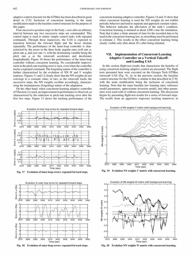
adaptive control structure for the GTMax has been described in greatdetail in [7,9]. Inclusion of concurrent learning is the mainmodificationmade to the baseline control structure for the purpose ofthis paper.

Four successive position steps in the body x axis after an arbitraryinterval between any two successive steps are commanded. Thiscontrol input is used to mimic simple control tasks with repeatedcommands. Through these maneuvers, the UAS is expected totransition between the forward flight and the hover domainrepeatedly. The performance of the inner-loop controller is char-acterized by the errors in the three body angular rates (roll rate p,pitch rate q, and yaw rate r), with the dominating variable being thepitch rate q as the rotorcraft accelerates and decelerateslongitudinally. Figure 10 shows the performance of the inner-loopcontroller without concurrent learning. No considerable improve-ment in the pitch-rate tracking error is seen, even when the controllertracks a repeated command. The forgetting nature of the controller isfurther characterized by the evolution of NN W and V weightsmatrices. Figures 11 and 12 clearly show that the NNweights do notconverge to a constant value; in fact, as the rotorcraft tracks thesuccessive steps, the NN weights oscillate accordingly, character-izing the instantaneous (forgetting) nature of the adaptation.

On the other hand, when concurrent-learning adaptive controllerof Theorem 2 is used, an improvement in performance is observed, ascharacterized by the reduction in pitch-rate tracking error after thefirst two steps. Figure 13 shows the tracking performance of the

concurrent-learning adaptive controller. Figures 14 and 15 show thatwhen concurrent learning is used the NN weights do not exhibitperiodic behavior and tend to separate and approach constant values.This behavior indicates the alleviation of the rank-1 condition.Concurrent learning is initiated at about 2200 s into the simulation.Note that it takes a finite amount of time for the recorded data to beused in the concurrent-learning law, as smoothingmust be performedto estimate �x. This results in the effect concurrent learning beingclearly visible only after about 20 s after being initiated.

VII. Implementation of Concurrent-LearningAdaptive Controller on a Vertical-Takeoff-

and-Landing UAS

In this section flight-test results that characterize the benefits ofusing concurrent-learning adaptive control are presented. The flighttests presented here were executed on the Georgia Tech GTMaxrotorcraft UAS (Fig. 9). As in the previous section, the baselinecontrol structure for the GTMax is similar to that described in [7,9],with the main modification being the inclusion of concurrentlearning. Note that the same baseline law learning rates, referencemodel parameters, approximate inversion model, and other param-eters were used with or without concurrent learning. The discussionbegins by presenting flight-test results for a series of forward steps.The results from an aggressive trajectory tracking maneuver, in

3370 3380 3390 3400 3410 3420 3430 3440 3450 3460

-0.1-0.05

00.05

0.1

Err

or in

p (

rad/

s)

Evolution of inner loop errors for repeated forward steps

3370 3380 3390 3400 3410 3420 3430 3440 3450 3460

-0.1-0.05

00.05

0.1

Err

or in

q (

rad/

s)

3370 3380 3390 3400 3410 3420 3430 3440 3450 3460

-0.1-0.05

00.05

0.1

Err

or in

r (

rad/

s)

Time (sec)

Fig. 17 Evolution of inner-loop errors: repeated forward steps.

3370 3380 3390 3400 3410 3420 3430 3440 3450 3460-2

-1

0

1

2Evolution of outer loop errors for repeated forward steps

Err

or in

u (

ft/s)

3370 3380 3390 3400 3410 3420 3430 3440 3450 3460-2

-1

0

1

2

Err

or in

v (

ft/s)

3370 3380 3390 3400 3410 3420 3430 3440 3450 3460-2

-1

0

1

2

Err

or in

w (

ft/s)

Time (sec)

Fig. 18 Evolution of outer-loop errors: repeated forward steps.

3370 3380 3390 3400 3410 3420 3430 3440 3450 3460-3

-2

-1

0

1

2

3Evolution of NN weights V matrix (with background learning)

Time (sec)

NN

wei

ghts

V m

atrix

Fig. 19 Evolution NN weights V matrix with concurrent learning.

3370 3380 3390 3400 3410 3420 3430 3440 3450 3460-0.4

-0.3

-0.2

-0.1

0

0.1

0.2

0.3

0.4

0.5Evolution of NN weights W matrix (with background learning)

Time (sec)

NN

wei

ghts

W m

atrix

Fig. 20 Evolution NN weights W matrix with concurrent learning.


which the UAS tracks an elliptical trajectory with aggressivevelocity, and acceleration profiles are then presented.

A. Repeated Forward-Step Maneuvers

The repeated forward-step maneuvers are chosen to demonstrate asituation in which the controller performs a simple repeated task.Figure 16 shows the body-frame states from recorded flight data for achain of forward-step commands. Figures 17 and 18 show theevolution of inner- and outer-loop errors, respectively, for therepeated forward-step maneuvers. These results assert the stability(in the sense of UUB) of the concurrent-learning controller ofTheorem 2.

Figures 19 and 20 show the evolution of NN weights as the rotor-craft tracks repeated steps using the concurrent-learning controller ofTheorem 2. Figures 21 and 22 show the evolution of NN weights asthe rotorcraft tracks another sequence of repeated steps withoutconcurrent learning. The NN V weights (Fig. 19) appear to approach

constant values when concurrent learning is used. This behavior canbe contrasted with Fig. 21, which shows that the NN V weightswithout concurrent learning do not appear to approach constantvalues. NNW weights for both cases remain bounded, with the maindifference being the increased separation in W weights whenconcurrent learning is used, indicating the alleviation of the rank-1condition. Furthermore, it is noted that the weights take on muchlarger values when using concurrent learning. This indicates thatconcurrent-learning adaptive law is searching for ideal weights inareas of the weight space that are never reached by the baselineadaptive without concurrent learning. The flight-test results alsoindicate an improvement in the error profile. In Fig. 18 it is seen thatthe lateral velocity tracking error reduces over repeated commands.These effects in combination indicate improved performance of theconcurrent-learning adaptive controller. These results are of parti-cular interest, since the maneuvers performed were conservative andthe baseline adaptive controller had already been extensively tuned.

4000 4005 4010 4015 4020 4025 4030 4035 4040 4045-0.5

-0.4

-0.3

-0.2

-0.1

0

0.1

0.2

0.3

0.4

0.5Evolution of NN weights W matrix

Time (sec)

NN

wei

ghts

W m

atrix

Fig. 22 Evolution of NN weights W matrix without concurrentlearning.

5250 5300 5350 5400 5450 5500 5550 5600-1

0

1Body velocity and accln

p ra

d/s

5250 5300 5350 5400 5450 5500 5550 5600-1

0

1

qrad

/s

5250 5300 5350 5400 5450 5500 5550 5600-1

0

1

r ra

d/s

5250 5300 5350 5400 5450 5500 5550 5600-100

0

100

u ft/

s

5250 5300 5350 5400 5450 5500 5550 5600-20

0

20

v ft/

s

5250 5300 5350 5400 5450 5500 5550 5600-20

0

20

w ft

/s

Time (sec)

Fig. 23 Recorded inner- and outer-loop states when repeatedly tracking aggressive trajectories.

4000 4005 4010 4015 4020 4025 4030 4035 4040 4045-0.04

-0.02

0

0.02

0.04

0.06

0.08

0.1

0.12Evolution of NN weights V matrix

Time (sec)

NN

wei

ghts

V m

atrix

Fig. 21 Evolution NN weights V matrix without concurrent learning.


B. Aggressive Trajectory Tracking Maneuver

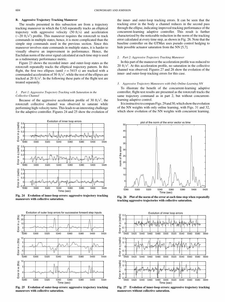
The results presented in this subsection are from a trajectorytracking maneuver in which the UAS repeatedly tracks an ellipticaltrajectory with aggressive velocity (50 ft=s) and acceleration( 20 ft=s2) profile. This maneuver requires the rotorcraft to trackcommands in multiple states; hence, it is more complicated than thesimple step commands used in the previous section. Since thismaneuver involves state commands in multiple states, it is harder tovisually observe an improvement in performance. Hence, theEuclidian norm of the error signal calculated at each time step is usedas a rudimentary performance metric.

Figure 23 shows the recorded inner- and outer-loop states as therotorcraft repeatedly tracks the elliptical trajectory pattern. In thisflight, the first two ellipses (until t� 5415 s) are tracked with acommanded acceleration of 30 ft=s2, while the rest of the ellipses aretracked at 20 ft=s2. In the following these parts of the flight test aretreated separately.

1. Part 1: Aggressive Trajectory Tracking with Saturation in the

Collective Channel

Because of the aggressive acceleration profile of 30 ft=s2, therotorcraft collective channel was observed to saturate whileperforming high-velocity turns. This leads to an interesting challengefor the adaptive controller. Figures 24 and 25 show the evolution of

the inner- and outer-loop tracking errors. It can be seen that thetracking error in the body u channel reduces in the second passthrough the ellipse, indicating improved tracking performance of theconcurrent-learning adaptive controller. This result is furthercharacterized by the noticeable reduction in the norm of the trackingerror calculated at every time step, as shown in Fig. 26. Note that thebaseline controller on the GTMax uses pseudo control hedging tohide possible actuator saturation from the NN [5,7].

2. Part 2: Aggressive Trajectory Tracking Maneuver

In this part of themaneuver the acceleration profilewas reduced to20 ft=s2. At this acceleration profile, no saturation in the collectivechannel was observed. Figures 27 and 28 show the evolution of theinner- and outer-loop tracking errors for this case.

3. Aggressive Trajectory Maneuvers with Only Online-Learning NN

To illustrate the benefit of the concurrent-learning adaptivecontroller, flight-test results are presented as the rotorcraft tracks thesame trajectory command as in part 2, but without concurrent-learning adaptive control.

It is instructive tocompareFigs.29and30,whichshowtheevolutionof the NN weights with only online learning, with Figs. 31 and 32,which show evolution of the NN weights with concurrent learning.

5280 5300 5320 5340 5360 5380 5400 5420-0.2

0

0.2

0.4

0.6Evolution of inner loop errors

Err

or in

p (

rad/

s)

5280 5300 5320 5340 5360 5380 5400 5420-0.2

0

0.2

0.4

0.6

Err

or in

q (

rad/

s)

5280 5300 5320 5340 5360 5380 5400 5420-0.2

0

0.2

0.4

0.6

Err

or in

r (

rad/

s)

Time (sec)

Fig. 24 Evolution of inner-loop errors: aggressive trajectory tracking

maneuvers with collective saturation.

5280 5300 5320 5340 5360 5380 5400 5420-10

0

10

20

30Evolution of outer loop errors for successive forward step inputs

Err

or in

u (

ft/s)

5280 5300 5320 5340 5360 5380 5400 5420-10

-5

0

5

10

Err

or in

v (

ft/s)

5280 5300 5320 5340 5360 5380 5400 5420-5

0

5

10

Err

or in

w (

ft/s)

Time (sec)

Fig. 25 Evolution of outer-loop errors: aggressive trajectory tracking

maneuvers with collective saturation.

5280 5300 5320 5340 5360 5380 5400 54200

5

10

15

20

25

30

35

40

45

50plot of the norm of the error vector vs time

Time (sec)

norm

of t

he e

rror

Fig. 26 Plot of the norm of the error at each time step when repeatedly

tracking aggressive trajectories with collective saturation.

5400 5420 5440 5460 5480 5500 5520 5540 5560 5580 5600-0.2

-0.1

0

0.1

0.2Evolution of inner loop errors

Err

or in

p (

rad/

s)

5400 5420 5440 5460 5480 5500 5520 5540 5560 5580 5600-0.2

-0.1

0

0.1

0.2

Err

or in

q (

rad/

s)

5400 5420 5440 5460 5480 5500 5520 5540 5560 5580 5600-0.2

-0.1

0

0.1

0.2

Err

or in

r (

rad/

s)

Time (sec)

Fig. 27 Evolution of inner-loop errors: aggressive trajectory tracking

maneuvers without collective saturation.


5400 5420 5440 5460 5480 5500 5520 5540 5560 5580 5600-5

0

5

10Evolution of outer loop errors

Err

or in

u (

ft/s)

5400 5420 5440 5460 5480 5500 5520 5540 5560 5580 5600-5

0

5

10

Err

or in

v (

ft/s)

5400 5420 5440 5460 5480 5500 5520 5540 5560 5580 5600-5

0

5

10

Err

or in

w (

ft/s)

Time (sec)

Fig. 28 Evolution of outer-loop errors: aggressive trajectory tracking

maneuvers without collective saturation.

5590 5600 5610 5620 5630 5640 5650 5660-0.8

-0.6

-0.4

-0.2

0

0.2

0.4

0.6

0.8


Time (sec)

NN

wei

ghts

V m

atrix

Fig. 29 Evolution ofNNVmatrixweights without concurrent-learning

adaptation.

5590 5600 5610 5620 5630 5640 5650 5660-1.5

-1

-0.5

0

0.5

1

1.5

2

2.5Evolution of NN weights W matrix (with background learning)

Time (sec)

NN

wei

ghts

W m

atrix

Fig. 30 Evolution of NN W matrix weights without concurrent-

learning adaptation.

5280 5300 5320 5340 5360 5380 5400 5420-6

-4

-2

0

2

4

6


Time (sec)

NN

wei

ghts

V m

atrix

Fig. 31 Evolution of NNVmatrix weights as theUAS tracks aggressive

trajectory with concurrent-learning adaptation.

5280 5300 5320 5340 5360 5380 5400 5420-3

-2

-1

0

1

2

3

4Evolution of NN weights W matrix (with background learning)

Time (sec)

NN

wei

ghts

W m

atrix

Fig. 32 Evolution of NN W matrix weights as the UAS tracks anaggressive trajectory with concurrent-learning adaptation.

5590 5600 5610 5620 5630 5640 5650 56600

5

10

15

20

25

30


Time (sec)

norm

of t

he e

rror

Fig. 33 Evolution of the norm of the tracking-error vector without

concurrent learning when tracking aggressive trajectories.


Although absolute convergence ofweights is not seen, it is interestingto note thatwhenusing concurrent learning theweights tend to be lessoscillatory. Also, when using concurrent learning, the adaptation isretained (that is, the weights do not approach zero) when the UAS ishovering between two successive maneuvers. Furthermore, theweights take on different values when using concurrent learning.Figure33showstheplotof thetracking-errornormwithoutconcurrentlearning evaluated at each time step, and Fig. 34 shows the plot of thetracking-error normwith current learning. The peaks in the tracking-error norms in these figures represent the beginning of a maneuver.Note thatFig.33containsonlyonepeak,asdataforonlyonemaneuverwithout concurrent learning were recorded, whereas Fig. 34 containstwo peaks, as data for two consecutive maneuvers were recorded.Contrasting thepeakof the tracking-errornorminFig.33withFig.34,it can be seen that the norm of the error vector is much higher withoutconcurrent learning, indicating that the combined online- andconcurrent-learning adaptive controller has improved trajectorytracking performance.

VIII. Conclusions

In this paper theory and flight-test results for a concurrent-learningadaptive control algorithm were presented. The ultimate bounded-ness of all system signals using Lyapunov-like stability analysis forthe presented adaptive control law in the framework of approximatemodel reference adaptive control was shown. Concurrent learningsimulates memory by recording interesting data points and storingthem in a history stack. The novel aspect of this learning law is itsability to adapt using current as well as stored data without affectingthe responsiveness of the adaptive law to current data. Concurrentlearning achieves this by restricting the training on recorded data tothe null-space of the training based on current data. Concurrentlearning also allows the use of direct training information, which canbe used to improve the performance of the adaptive controller. It wasalso shown that concurrent learning alleviates the rank-1 condition oftraditional backpropagation-based NN training laws that use onlycurrent data for adaptation. Furthermore, since the choice of thebaseline adaptive law and the projection matrix does not affect thestability properties of the concurrent-learning adaptive law, it isexpected that the concurrent-learning methodology can be furthergeneralized to other adaptive schemes.

Another contribution of this paper was the presentation of flight-test results with concurrent-learning adaptive controllers on arotorcraft unmanned aerial vehicle. The flight-test results ascertainthat all states remain uniformly ultimately bounded when usingconcurrent-learning adaptation. Expected improvement in trackingperformance was noted. Furthermore, the evolutions of the neuralnetwork W and V matrix weights were observed to have different

characteristics when concurrent learning was employed, includingweight separation, a tendency toward weight convergence in somecases, and different numerical values of the adaptive weights. Thisdifference in neural network weight behavior demonstrates the effectof overcoming the rank-1 condition. Because of the fact that othertraining algorithms are enabled by the stability proof, and sincemanyother ways for selecting data points can be developed, this can beachieved even more consistently by improved implementation.

Appendix: Optimal Fixed-Point Smoothing

Numerical differentiation for estimation of state derivates suffersfrom high sensitivity to noise. An alternate method is to use aKalman-filter-based approach. Let x be the state of the system, let _xbe its first derivative, and consider the following system:

_x�xx:::

24

35� 0 1 0

0 0 1

0 0 0

24

35 x

_x�x

24

35 (A1)

Suppose that x and _x are available as sensor measurements, thenusing the above system, optimal fixed-point smoothing can be usedto estimate �x from available noisy measurements [25].

Optimal fixed-point smoothing is a non-real-time method forarriving at a state estimate at some time t, where 0 � t � T, by usingall available data up to time T. Optimal smoothing combines aforward filter that operates on all data before time t and a backwardfilter that operates on all data after time t to arrive at an estimate of thestate that uses all the available information. This Appendix presentsbrief information on implementation of optimal fixed-pointsmoothing; the interested reader is referred to Gelb [25] for furtherdetails. For ease of implementation on modern avionics, the relevantequations are presented in the discrete form. Let xkjN denote theestimate of the state x� � x _x �x �T , let Zk denote the mea-surements, let (�) denote predicted values, and let (�) denotecorrected values. Then the forward Kalman filter equations can begiven as follows:

�k � e

0 1 0

0 0 1

0 0 0

24

35 dt

0@

1A

(A2)

zk �1 0 0

0 1 0

� � x_x�x

24

35 (A3)

x k�� kxk�1 (A4)

Pk�� kPk�1�Tk �Qk (A5)

Kk � Pk��HTk �HkPk��HT

k � Rk��1 (A6)

x k�� xk�� Kk�Zk �Hkxk�� (A7)

Pk�� I � KkHk�Pk�� (A8)

The smoothed state estimate can be given as

x kjN � xkjN�1 � BN �xN�� xN�� (A9)

where xkjk � xk, N � k� 1; k� 2; . . ., and

BN ��N�1i�k Pi��T

i P�1i�1�� (A10)

5420 5440 5460 5480 5500 5520 5540 5560 5580 56000

5

10

15

20

25

30


Time (sec)

norm

of t

he e

rror

Fig. 34 Evolution of the norm of the tracking-error vector withconcurrent learning when tracking aggressive trajectories.


The smoothed error covariance matrix is propagated as

PkjN � PkjN�1 � BN �Pk�� Pk��BTN (A11)

where Pkjk � Pk��.

Acknowledgments

This work was supported in part by National Science Foundationgrant ECS-0238993 and NASA Research Announcement NNX08AD06A. The authors also thank the members of the GeorgiaInstitute of Technology’s unmanned aerial vehicle research facilityfor their support in flight-testing activities. Particularly, the authorswish to thank Suresh Kannan, Jeong Hur, R. Wayne Pickell, HenrikChristophersen, Nimord Rooz, AllenWu, H. Claus Christmann, andM. Scott Kimbrell.

References

[1] Lewis, F. L., “Nonlinear Network Structures for Feedback Control,”Asian Journal of Control, Vol. 1, Dec. 1999, pp. 205–228.doi:10.1111/j.1934-6093.1999.tb00021.x

[2] Kim, Y. H., and Lewis, F. L.,High Level Feedback Control with NeuralNetworks, World Scientific Series in Robotics and Intelligent Systems,Vol. 21, World Scientific, Singapore, 1998.

[3] Patiño, D. H., Carelli, R., and Kuchen, B. R., “Neural Networks forAdvanced Control of Robot Manipulators,” IEEE Transactions on

Neural Networks, Vol. 13, No. 2, March 2002, pp. 343–354.doi:10.1109/72.991420

[4] Calise, A., Hovakimyan, N., and Idan, M., “Adaptive Output FeedbackControl of Nonlinear Systems Using Neural Networks,” Automatica,Vol. 37, No. 8, Aug. 2001, pp. 1201–1211.doi:10.1016/S0005-1098(01)00070-X

[5] Johnson, E. N., “Limited Authority Adaptive Flight Control,” Ph.D.Thesis, Georgia Inst. of Technology, Atlanta, 2000.

[6] Johnson, E. N., and Calise, A., “Limited Authority Adaptive FlightControl for Reusable Launch Vehicles,” Journal of Guidance, Control,and Dynamics, Vol. 26, No. 6, pp. 906–913.doi:10.2514/2.6934, 2003

[7] Johnson, E. N., and Kannan, S. K., “Adaptive Trajectory Control forAutonomous Helicopters,” Journal of Guidance, Control, and

Dynamics, Vol. 28, No. 3, May–June 2005, pp. 524–538.doi:10.2514/1.6271

[8] Johnson, E., Turbe, M., and Wu, A., edited by S. Kannan, “FlightResults of Autonomous Fixed-Wing UAS Transitions to and fromStationary Hover,” AIAA Guidance, Navigation, and ControlConference, AIAA Paper 2006-6775, Aug. 2006.

[9] Kannan, S. K., “Adaptive Control of Systems in Cascade withSaturation,” Ph.D. Thesis, Georgia Inst. of Technology, Atlanta, 2005.

[10] Hovakimyan, N., Yang, B. J., and Calise, A., “Adaptive OutputFeedback Control Methodology Applicable to Non-Minimum PhaseNonlinear Systems,” Automatica, Vol. 42, No. 4, 2006, pp. 513–522.doi:10.1016/j.automatica.2005.11.001

[11] Cao, C., and Hovakimyan, N., “Design and Analysis of a Novel L1

Adaptive Control Architecture with Guaranteed Transient Perform-ance,” IEEE Transactions on Automatic Control, Vol. 53, No. 2, 2008,pp. 586–590.doi:10.1109/TAC.2007.914282

[12] Lavretsky, E., and Wise, K., “Adaptive Flight Control of Manned/Unmanned Military Aircraft,” Proceedings of the American Control

Conference, June 2005.[13] Nguyen, N., Krishnakumar, K., Kaneshige, J., and Nespeca, P.,

“Dynamics and Adaptive Control for Stability Recovery of DamagedAsymmetric Aircraft,” AIAA Guidance, Navigation, and ControlConference, AIAA Paper 2006-6049, Keystone, CO, Aug. 2006.

[14] Ioannou, P., and Sun, J.,Robust AdaptiveControl, Prentice–Hall, UpperSaddle River, NJ, 1996.

[15] Gang, T., Adaptive Control Design and Analysis, Wiley, New York,2003.

[16] Boyd, S., and Sastry, S., “Necessary and Sufficient Conditions forParameter Convergence in Adaptive Control,” Automatica, Vol. 22,No. 6, 1986, pp. 629–639.doi:10.1016/0005-1098(86)90002-6

[17] Narendra, K., and Annaswamy, A., “A New Adaptive Law for RobustAdaptation without Persistent Excitation,” IEEE Transactions on

Automatic Control, Vol. 32, No. 2, Feb. 1987, pp. 134–145.doi:10.1109/TAC.1987.1104543

[18] Haykin, S., Neural Networks a Comprehensive Foundation, 2nd ed.,Prentice–Hall, Upper Saddle River, NJ, 1998.

[19] Ponzyak, A. S., Sanchez, E. N., and Yu, W., Differential Neural

Networks for Robust Nonlinear Control, Identification, State

Estimation, and Trajectory Tracking, World Scientific, Singapore,2001.

[20] Suykens, J. A. K., Vandewalle, J. P. L., and DeMoor, B. L. R.,ArtificialNeural Networks for Modeling and Control of Non-Linear Systems,Kluwer Academic, Dordrecht, The Netherlands, 1996.

[21] Ioannou, P. A., and Kokotovic, P. V., Adaptive Systems with Reduced

Models, Springer–Verlag, Berlin, 1983.[22] Volyanskyy, K., Calise, A. J., Yang, B. J., and Lavretsky, E., “An Error

Minimization Method in Adaptive Control,” AIAA GuidanceNavigation and Control Conference, AIAA Paper 2006-6346,Keystone, CO, 2006.

[23] Hornik, K., Stinchcombe, M., and White, H., “Multilayer FeedforwardNetworks are Universal Approximators,” Neural Networks, Vol. 2,1989, pp. 359–366.doi:10.1016/0893-6080(89)90020-8

[24] Strang, G., Linear Algebra and its Applications, 3rd ed., ThomsonLearning, San Diego, CA, 1988.

[25] Gelb, A., Applied Optimal Estimation, MIT Press, Cambridge, MA,1974.

[26] Hadad, W., and Chellebaonia, V., Nonlinear Dynamical Systems andControl: A Lyapunov Based Approach, Princeton Univ. Press,Princeton, NJ, 2006.

[27] Khalil, H., Nonlinear Systems, 3rd ed., Prentice–Hall, Upper SaddleRiver, NJ, 2001.

[28] Berberian, S. K., Introduction to Hilbert Spaces, AMS Chelsea,New York, 1976.


http://dx.doi.org/10.1111/j.1934-6093.1999.tb00021.x

http://dx.doi.org/10.1109/72.991420

http://dx.doi.org/10.1016/S0005-1098(01)00070-X

http://dx.doi.org/10.2514/2.6934

http://dx.doi.org/10.2514/1.6271

http://dx.doi.org/10.1016/j.automatica.2005.11.001

http://dx.doi.org/10.1109/TAC.2007.914282

http://dx.doi.org/10.1016/0005-1098(86)90002-6

http://dx.doi.org/10.1109/TAC.1987.1104543

http://dx.doi.org/10.1016/0893-6080(89)90020-8

Theory and Flight-Test Validation of a Concurrent-Learning

Documents

Transcript of Theory and Flight-Test Validation of a Concurrent-Learning