Experimental and Computational Steady and Unsteady Transonic ...
THEORY AND EXPERIMENTAL EVALUATION OF A
CONSISTENT STEADY-STATE KINETIC MODEL FOR
2-D CONDUCTIVE STRUCTURES IN IONOSPHERIC
PLASMAS WITH APPLICATION TO BARE
ELECTRODYNAMIC TETHERS IN SPACE
by
Eric Choiniere
A dissertation submitted in partial fulfillmentof the requirements for the degree of
Doctor of Philosophy(Electrical Engineering)
in The University of Michigan2004
Doctoral Committee:
Professor Brian E. Gilchrist, ChairAssistant Professor Sven G. BilenProfessor Iain BoydProfessor Alec D. GallimoreProfessor Kamal Sarabandi

©Eric Choiniere
All Rights Reserved2004

A mon amour, Isabelle, pour sa patience et son support,
et a la memoire de ma grand-mere Bernadette.
ii

ACKNOWLEDGMENTS
First, I would like to thank my research advisor and committee chair, Professor Brian
Gilchrist, for allowing me on board in September of 1999 when I first stepped foot in his
office, for making so many great opportunities happen during my years in Ann Arbor, and
for all of his support throughout this exciting, difficult, and rewarding journey. I really
appreciate the freedom and trust you have given me throughout the years, as well as the
friendly atmosphere that you have fostered within the SETS group. I look forward to
collaboration in the future.
I would also like to thank the other members of my thesis committee, Prof. Sven Bilen,
Prof. Iain Boyd, Prof. Alec Gallimore and Prof. Sarabandi, for accepting to judge this
work and for their guidance. Special thanks go to Prof. Bilen for teaching me the ropes
of experimental work while he was working as a Postdoc at Michigan, as well as for his
guidance with the English language throughout several co-authored papers and this thesis.
I would like to thank Prof. Gallimore for his essential support of our experimental work
in the Large Vacuum Test Facility, and for having given a second life to this outstanding
vacuum test facility.
I would like to thank my colleagues of the Space Electrodynamics and Tether Systems
(SETS) group for their assistance and guidance throughout the years, for all the insightful
discussions, for the entertaining and politically-charged debates, and for their friendship.
Thanks to Dave Morris, Chris Davis, Boon Lim, Brent West, Hannah Goldberg, Chris
iii

Deline, and Keith Fuhrhop. Special thanks to Keith for all his help preparing and analyzing
laboratory tests.
I am grateful for scholarship support provided by a 2-year Postgraduate Scholarship
from the Natural Sciences and Engineering Research Council of Canada, two Fessenden
Graduate Awards from the Communications Research Centre and Industry Canada, a 1-
year Departmental Fellowship from the Electrical Engineering and Computer Science de-
partment, and a 1-year Rackham Predoctoral Fellowship from the Horace H. Rackham
School of Graduate Studies. These fellowships not only allowed me to join the Ph.D. pro-
gram within such a great institution as the University of Michigan, they also gave me the
liberty to take risks in undertaking the development of a new computational plasma model,
which would probably not have been possible through other types of funding resources.
I would like to acknowledge the support of NASA for part of the experimental portion of
this work through the STEP-Airseds project. I would also like to acknowledge the support
of Tethers Unlimited, Inc. with special thanks to Rob Hoyt, Bryan Minor and Nestor
Voronka. Thank you for providing new and exciting opportunities for the application of the
KiPS models to the remediation of radiation belts. I look forward to future collaboration
on this and other exciting space projects.
From the Plasmadynamics and Electric Propulsion Laboratory, I would like to thank,
in addition to Professor Alec Gallimore, all of the students and staff members who have
assisted and guided in one way or another myself and other members of the Space Elec-
trodynamic and Tether Systems group during several electrodynamic tether sample testing
sessions. Thanks to Tim Smith, Dan Hermann, Mitchell Walker, Brian Beal, Jon Van No-
ord, and Travis Patrick.
Several fellow members of the Radiation Laboratory have provided their technical as-
sistance, guidance or friendship during my stay at Michigan. I would like to thank in
iv

particular Stephane Legault, Hanh Pham, Mark Casciato, Lee Harle, Brian Hornbuckle,
Valdis Liepa and Nadib Nashashibi.
Special thanks go to several researchers in the space plasma community with whom I
have had some very insightful exchanges and discussions: Prof. James Laframboise, Dr.
Ira Katz, Prof. Juan Sanmartın, Prof. Manual Martınez-Sanchez, Dr. Tatsuo Onishi, and
Dr. Dave Cook.
Several staff members have indirectly contributed to this thesis by making things run
smoother for me as a graduate student. In the Space Physics Research Laboratory, I would
like to thank Charles Navarre (“Chuck”) for his help in the machine shop, Clinton Lee for
putting up with all my special backup needs, and Melissa Lee, our outstanding secretary.
For their flawless administrative support, I would like to thank Susan Charnley, Mary Eyler
and Karen Kirchener from the Radiation Laboratory and Beth Stalnaker from EECS.
The highly computational nature of the present work relies on the existence and avail-
ability of large parallel computing resources. I would like to thank Mark Giuffrida, di-
rector of the Computer Aided Engineering Network, for his collaboration and flexibility in
the deployment and operation of a powerful opportunistic computing platform for plasma
simulations on the CAEN network.
Authors of free software provide an invaluable contribution to the scientific community.
I would like to specifically acknowledge Frederic Hecht, the author of the Bidimensional
Anisotropic Mesh Generator (BAMG), and all the authors of the Parallel Virtual Machine
(PVM) at Oak Ridge National Laboratory. I am also grateful to Leslie Lamport, the author
of the most essential thesis writing tool, LATEX.
I would like to thank my friends from up in Quebec for their support and continuous
friendship despite the 12-hour drive that separated us during almost five years. Merci pour
votre amitie.
v

I acknowledge my family as well as my wife’s family for their support and patience
throughout the past years spent in the United States. I would especially like to thank my
parents for encouraging me to reach for my dreams. Chere soeur, I have not forgotten your
promise to read my thesis once completed ! I only wish my grandmother Bernadette had
lived to see this work completed.
Last, but not least, I wish to thank my wife Isabelle for her love, companionship and
endurance throughout the past 5 years. You have largely contributed to the success of this
journey. Merci mon amour!
Eric ChoiniereSeptember 24, 2004
vi

ABSTRACT
THEORY AND EXPERIMENTAL EVALUATION OF A CONSISTENTSTEADY-STATE KINETIC MODEL FOR 2-D CONDUCTIVE
STRUCTURES IN IONOSPHERIC PLASMAS WITH APPLICATIONTO BARE ELECTRODYNAMIC TETHERS IN SPACE
byEric Choiniere
Chair: Brian E. Gilchrist
A steady-state kinetic computational model is developed, allowing for self-consistent
simulations of collisionless, unmagnetized flowing plasmas in a vast region surrounding
any two-dimensional conductive object. An optimization approach is devised based on a
stable, noise-robust Tikhonov-regularized Newton method. Dynamic, adaptive, unstruc-
tured meshing allows arbitrary geometries and adequate resolution of plasma sheath fea-
tures. A 1-D cylindrical solver (KiPS-1D) and a full 2-D solver (KiPS-2D) were developed,
the latter using coarse-grained parallelism.
This technique is applied to investigate various applications of special and fundamen-
tal importance, principally for space plasmas, although not limited as such. This thesis
addresses new simulations and experiments relevant to space borne electrodynamic teth-
ers for propellantless propulsion and for the remediation of radiation belts through charge
precipitation, as well as to Langmuir probes for plasma diagnostic in flowing plasmas.
Here, the existing set of plasma sheath profiles and current collection characteristics
for round cylinders in stationary plasmas is extended to large bias potentials. Interfer-
vii

ence effects between two parallel cylinders are shown to exist for spacings upward of 20
times the single-cylinder sheath radius, and an optimal spacing equal to the single-cylinder
sheath radius maximizes the sheath area, a finding qualitatively supported by our new ex-
perimental data on electron-collecting thin slotted tapes. Also, a thin conductive solid tape
is shown to have an equal-capacitance circular radius of about 0.29 times its width. Its
predicted collected current characteristic as a function of width approximately agrees with
experimental measurements. Further, it has a lower current collection capability than the
equal-capacitance circular cylinder.
For ion-attracting cylinders, ionospheric plasma representative of an altitude of 1500
km with a flow energy on the order of the thermal energy is shown to cause significant
sheath asymmetries, reducing the sheath radius and current collection by about 30%. For
electron-attracting cylinders, a mesosonic flow is experimentally shown to significantly
enhance electron collection. This cannot be predicted by a collisionless model and may be
due to an elongation of the ram-side pre-sheath into a collisional zone for electrons.
viii

TABLE OF CONTENTS
DEDICATION . . . . . . . . . . . . . . . . . . . . . . . . . . . . . . . . . . . . . ii
ACKNOWLEDGMENTS . . . . . . . . . . . . . . . . . . . . . . . . . . . . . . . iii
ABSTRACT . . . . . . . . . . . . . . . . . . . . . . . . . . . . . . . . . . . . . . vii
LIST OF TABLES . . . . . . . . . . . . . . . . . . . . . . . . . . . . . . . . . . . xiv
LIST OF FIGURES . . . . . . . . . . . . . . . . . . . . . . . . . . . . . . . . . . xv
LIST OF ALGORITHMS . . . . . . . . . . . . . . . . . . . . . . . . . . . . . . .xxiii
LIST OF APPENDICES . . . . . . . . . . . . . . . . . . . . . . . . . . . . . . . xxiv
CHAPTERS
1 Introduction, Background and Previous Research . . . . . . . . . . . . . . 11.1 Motivation and Definition of the Problem . . . . . . . . . . . . . . 1
1.1.1 Bare Electrodynamic Tethers for Space Propulsion . . . . 21.1.2 Bare Electrodynamic Tethers for Ionospheric High-Energy
Charge Precipitation (“Electrostatic” Tethers) . . . . . . . 51.1.3 Plasma Diagnostics Probes . . . . . . . . . . . . . . . . . 61.1.4 Other Applications . . . . . . . . . . . . . . . . . . . . . 71.1.5 Description of the Problem & Regimes of interest . . . . . 8
1.2 Cylindrical Plasma Probes: Background and Literature Review . . 111.2.1 Stationary plasmas . . . . . . . . . . . . . . . . . . . . . 12
1.2.1.1 Thin Sheath Limit . . . . . . . . . . . . . . . . 131.2.1.2 Orbital-Motion Limit (“Thick” Sheath Limit) . . 141.2.1.3 Numerical Approaches for Arbitrary Probe Sizes 16
1.2.2 Flowing Plasmas . . . . . . . . . . . . . . . . . . . . . . 171.2.2.1 Treatments Based on a Symmetric Potential
Profile Assumption . . . . . . . . . . . . . . . . 171.2.2.2 Consistent Numerical Treatments . . . . . . . . 18
1.2.2.2.1 Steady-State Kinetic Treatments . . 181.2.2.2.2 Particle-in-Cell Treatment . . . . . . 19
1.3 Summary of Research Contributions . . . . . . . . . . . . . . . . 19
ix

1.3.1 A Self-Consistent Steady-State Kinetic Model for Arbi-trary 2-D Conductive Structures in Flowing Plasmas . . . . 20
1.3.2 New Simulation Results . . . . . . . . . . . . . . . . . . . 211.3.3 New Experimental Results . . . . . . . . . . . . . . . . . 22
1.4 Dissertation Overview . . . . . . . . . . . . . . . . . . . . . . . . 23
2 Steady-State Poisson–Vlasov Model: Theory and Implementation . . . . . 252.1 Basic Assumptions . . . . . . . . . . . . . . . . . . . . . . . . . 272.2 Poisson–Vlasov Representation of Collisionless Plasmas . . . . . 332.3 Finite-Element Poisson Solver . . . . . . . . . . . . . . . . . . . 36
2.3.1 1-D Cylindrical Implementation . . . . . . . . . . . . . . 372.3.2 2-D Implementation . . . . . . . . . . . . . . . . . . . . . 41
2.3.2.1 Poisson Boundary Conditions . . . . . . . . . . 412.3.2.2 Finite-Element Formulation . . . . . . . . . . . 43
2.3.2.2.1 Formulation of the Outer BoundaryCondition . . . . . . . . . . . . . . 43
2.3.2.2.2 Formulation of the Internal FiniteElements . . . . . . . . . . . . . . . 46
2.4 Steady-State Vlasov Solver . . . . . . . . . . . . . . . . . . . . . 502.4.1 1-D Cylindrical Implementation . . . . . . . . . . . . . . 51
2.4.1.1 Approximating the Vlasov Functional fV in 1-D 522.4.1.2 Linearizing the 1-D Vlasov Solver . . . . . . . . 55
2.4.2 Full 2-D Implementation . . . . . . . . . . . . . . . . . . 562.4.2.1 Orbit Tracking and Analysis . . . . . . . . . . . 56
2.4.2.1.1 A Note on Segment-bound Trajec-tories . . . . . . . . . . . . . . . . . 62
2.4.2.2 Sampling the Velocity Distribution Function . . 622.4.2.3 Velocity Space Integration . . . . . . . . . . . . 65
2.4.2.3.1 Defining “Directional-Energy” Space 652.4.2.3.2 Numerical Integration in
“Directional-Energy” Space . . . . . 662.4.2.4 Linearizing the 2-D Vlasov Solver . . . . . . . . 70
2.5 Regularized Newton Iterative Poisson–Vlasov Scheme . . . . . . . 702.5.1 Top-level Iterative Scheme . . . . . . . . . . . . . . . . . 712.5.2 Conditioning and Quadrature Noise Issues . . . . . . . . . 732.5.3 Diagonal Preconditioning . . . . . . . . . . . . . . . . . . 752.5.4 Tikhonov “Progressive” Regularization . . . . . . . . . . . 762.5.5 Discrepancy Principle as Stopping Criteria . . . . . . . . . 812.5.6 Dynamic Step Size Control . . . . . . . . . . . . . . . . . 822.5.7 Dynamic Adaptive Quadrature Tolerance . . . . . . . . . . 85
2.6 Dynamic Adaptive Mesh Refinement . . . . . . . . . . . . . . . . 862.6.1 KiPS Cylindrical 1-D Implementation . . . . . . . . . . . 862.6.2 KiPS 2-D Implementation . . . . . . . . . . . . . . . . . 88
2.6.2.1 Meshing Software . . . . . . . . . . . . . . . . 882.6.2.2 Mesh Symmetry Axes . . . . . . . . . . . . . . 88
x
2.6.2.3 Mesh Refinement: Strategy & Metrics . . . . . . 892.6.2.4 Examples of Mesh Geometries Under Consid-
eration . . . . . . . . . . . . . . . . . . . . . . 912.6.2.4.1 Single Round Cylinder . . . . . . . 912.6.2.4.2 Tape Cylinder . . . . . . . . . . . . 922.6.2.4.3 Two Round Cylinders . . . . . . . . 93
2.7 Computer Implementation . . . . . . . . . . . . . . . . . . . . . . 942.7.1 General Philosophy . . . . . . . . . . . . . . . . . . . . . 942.7.2 Optimizing & Parallelizing the Vlasov Solver . . . . . . . 952.7.3 Present Parallel Computing Platform . . . . . . . . . . . . 962.7.4 Alternative Parallel Computing Platforms . . . . . . . . . 96
3 Experimental Investigation of Electron-Collecting TetherSamples in a Mesosonic Xenon Plasma . . . . . . . . . . . . . . . . . . . 98
3.1 Background . . . . . . . . . . . . . . . . . . . . . . . . . . . . . 983.2 Design and Assembly of Solid and Slotted Tape Tether Guarded
Samples . . . . . . . . . . . . . . . . . . . . . . . . . . . . . . . 993.3 Vacuum Chamber Setup and Plasma Source Characteristics . . . . 1053.4 Plasma Parameter Measurements Using Negatively-Biased Lang-
muir Probes . . . . . . . . . . . . . . . . . . . . . . . . . . . . . 1083.5 Experimental Results & Analysis . . . . . . . . . . . . . . . . . . 110
3.5.1 Reference Cylinder . . . . . . . . . . . . . . . . . . . . . 1113.5.2 Solid Tapes . . . . . . . . . . . . . . . . . . . . . . . . . 1123.5.3 Slotted Tapes . . . . . . . . . . . . . . . . . . . . . . . . 1143.5.4 Comparison of the Solid and Slotted Tapes . . . . . . . . . 116
3.6 Present Status and Conclusions . . . . . . . . . . . . . . . . . . . 120
4 Simulation Results and Validation . . . . . . . . . . . . . . . . . . . . . . 1224.1 Definition of Normalized Physical Quantities . . . . . . . . . . . . 1224.2 Single Round Cylinder in Stationary Plasma . . . . . . . . . . . . 126
4.2.1 Validation of Potential & Density Profiles at Low BiasVoltages . . . . . . . . . . . . . . . . . . . . . . . . . . . 126
4.2.2 Validation of Collected Current at Low Bias Voltages . . . 1304.2.3 Assessment of Collected Current at High Bias Voltages . . 1314.2.4 Plasma Profiles at High Voltages . . . . . . . . . . . . . . 133
4.2.4.1 Typical Plasma Profile from KiPS-1D . . . . . . 1344.2.4.2 Typical Two-Dimensional Plasma Structure
from KiPS-2D . . . . . . . . . . . . . . . . . . 1374.2.4.3 Profile dependence on Bias Potential and Cylin-
der Radius . . . . . . . . . . . . . . . . . . . . 1374.2.4.4 Variation of the Ion Velocity Distribution
Throughout the Sheath . . . . . . . . . . . . . . 1434.2.5 Sheath Radius at High Voltages . . . . . . . . . . . . . . . 146
4.3 Interference of Parallel Round Cylinders in a Stationary Plasma . . 1494.3.1 Treatment of Repelled Electrons . . . . . . . . . . . . . . 150
xi

4.3.2 Orbits of the Attracted Ions . . . . . . . . . . . . . . . . . 1504.3.2.1 Criteria for Trapped Orbits . . . . . . . . . . . . 1514.3.2.2 Examples of Ion Orbits . . . . . . . . . . . . . . 152
4.3.3 Inspection of the 2-D Sheath Structure . . . . . . . . . . . 1544.3.4 Definition of an Effective Sheath Area Concept . . . . . . 1704.3.5 Determination of the Effective Sheath Area of the Two-
Cylinder Configuration . . . . . . . . . . . . . . . . . . . 1714.3.6 Parametric Analysis of the Sheath Structure . . . . . . . . 1814.3.7 Interference Effect on Collected Current . . . . . . . . . . 186
4.4 Solid Tape Cylinder in Stationary Plasma: Current Collection . . . 1894.4.1 Equivalent Cylinder Radius and Collected Current: Theo-
retical Comparisons . . . . . . . . . . . . . . . . . . . . . 1894.4.2 Collected Current: Comparisons with Experimental Results 192
4.5 Flow Effects on Ion-Attracting Round Cylinder . . . . . . . . . . 1964.5.1 Criteria for Trapped Orbits . . . . . . . . . . . . . . . . . 1984.5.2 Treatment of Electrons . . . . . . . . . . . . . . . . . . . 1994.5.3 Validation with Existing Simulation Results . . . . . . . . 200
4.5.3.1 Ion Density Profile Validations . . . . . . . . . . 2004.5.3.2 Ion Current Collection Validations . . . . . . . . 203
4.5.4 Ionospheric Flow Effects at High Altitudes (H=1500 km) . 2064.5.4.1 Flow Energy at Altitude of Interest . . . . . . . 2064.5.4.2 Inspection of the Sheath Structure . . . . . . . . 2074.5.4.3 Plasma Flow Effects on Sheath Structure and
Dimensions . . . . . . . . . . . . . . . . . . . . 2234.5.4.4 Plasma Flow Effect on Ion Current Collection . . 226
4.6 Flow Effects on Electron-Attracting Round Cylinder . . . . . . . . 2274.6.1 Potential and Density Profiles . . . . . . . . . . . . . . . . 2284.6.2 Electron Current Collection . . . . . . . . . . . . . . . . . 237
4.7 Outline of Simulation Resource Requirements . . . . . . . . . . . 2424.7.1 1-D Cylindrical Implementation (KiPS-1D) . . . . . . . . 2424.7.2 2-D Cylindrical Implementation (KiPS-2D) . . . . . . . . 244
4.7.2.1 Processing Time . . . . . . . . . . . . . . . . . 2444.7.2.2 Random-Access Memory Requirements . . . . . 247
5 Conclusions and Recommendations for Future Research . . . . . . . . . . 2485.1 Summary and Conclusions of Research . . . . . . . . . . . . . . . 248
5.1.1 Self-Consistent Steady-State Kinetic Model . . . . . . . . 2485.1.2 Experimental Investigation of Electron-Collecting Tether
Samples . . . . . . . . . . . . . . . . . . . . . . . . . . . 2505.1.3 Important Simulation and Experimental Results . . . . . . 251
5.1.3.1 Ion-Attracting High-Voltage Single Cylinder inStationary Plasma . . . . . . . . . . . . . . . . 251
5.1.3.2 Interference Effects of Parallel Cylinders . . . . 2515.1.3.3 Geometry Effects of the Solid Tape Cylinder . . 2525.1.3.4 Plasma Flow Effects on Ion-Attracting Cylinder . 252
xii
5.1.3.5 Plasma Flow Effects on Electron-AttractingCylinder . . . . . . . . . . . . . . . . . . . . . 253
5.2 Recommendations for Future Research . . . . . . . . . . . . . . . 2535.2.1 Computational Modeling . . . . . . . . . . . . . . . . . . 2545.2.2 Experimental Testing . . . . . . . . . . . . . . . . . . . . 256
APPENDICES . . . . . . . . . . . . . . . . . . . . . . . . . . . . . . . . . . . . . 258
BIBLIOGRAPHY . . . . . . . . . . . . . . . . . . . . . . . . . . . . . . . . . . . 281
xiii

LIST OF TABLES
Table
1.1 Approximate plasma parameters for the main applications of interest. . . . 11
2.1 Decay rates of the radial electric field Ern = −∂Vxn
∂ rfor various circular
harmonic modes. . . . . . . . . . . . . . . . . . . . . . . . . . . . . . . . 42
2.2 Functional operators and corresponding numerical solvers. . . . . . . . . . 71
3.1 Effective diameter of the reference cylinder and effective widths of thethree solid tapes. . . . . . . . . . . . . . . . . . . . . . . . . . . . . . . . 101
3.2 Effective center-to-center line spacing as a function of sample porosity. . . 101
3.3 Operating parameters of the plasma source (P5 Hall thruster). . . . . . . . . 107
3.4 Variation of the measured plasma parameters as a function of distance fromthe Hall thruster. . . . . . . . . . . . . . . . . . . . . . . . . . . . . . . . . 108
xiv

LIST OF FIGURES
Figure
1.1 Example of an application of the electrodynamic space tether concept foruse as a station keeping device for the International Space Station. . . . . . 3
1.2 Geometry of the interaction of the electrodynamic tether and the radiationbelt. . . . . . . . . . . . . . . . . . . . . . . . . . . . . . . . . . . . . . . 5
1.3 Four examples of the cylinder geometries under consideration. . . . . . . . 10
1.4 Normalized current characteristics in the thin sheath limit and orbital mo-tion limit. . . . . . . . . . . . . . . . . . . . . . . . . . . . . . . . . . . . 16
2.1 Example of the semi-analytical particle tracking process through the poten-tial mesh on a grid with normalized coordinates. . . . . . . . . . . . . . . . 59
2.2 Poisson–Vlasov operator comprised of both the Poisson and Vlasov solvers. 71
2.3 Tikhonov-regularized Newton iterative Poisson–Vlasov procedure. . . . . . 72
2.4 Sequence of refined meshes obtained for a single one-Debye-length-radiusround cylinder. . . . . . . . . . . . . . . . . . . . . . . . . . . . . . . . . 92
2.5 Sequence of refined meshes obtained for a tape cylinder. . . . . . . . . . . 93
2.6 Sequence of refined meshes for 2 parallel one-Debye-length-radius cylinders. 94
3.1 Drawing and description of the six guarded tether samples shown beforeassembly. . . . . . . . . . . . . . . . . . . . . . . . . . . . . . . . . . . . 100
3.2 Assemblies of the reference cylinder and tape guarded tether samples. . . . 102
3.3 Example of the ceramic attachment used on all solid and slotted tape samples.103
3.4 Pictures of three typical tether samples. . . . . . . . . . . . . . . . . . . . 104
xv

3.5 Experimental setup in the Large Vacuum Test Facility (LVTF) at the Plas-madynamics and Electric Propulsion Laboratory (PEPL). . . . . . . . . . . 106
3.6 Picture of the guarded sample support structure and the P5 Hall thrusterused as a high-speed plasma source. . . . . . . . . . . . . . . . . . . . . . 107
3.7 Schematic of the computer-controlled high-voltage test equipment setup. . . 109
3.8 Normalized I–V characteristics of parallel and perpendicular solid tapes. . . 113
3.9 Normalized I–V characteristics of parallel and perpendicular slotted tapes. . 115
3.10 Comparison of the I–V characteristics of solid and slotted tapes at 75 cm. . 117
3.11 Comparison of the I–V characteristics of solid and slotted tapes at 160 cm. . 118
3.12 Comparison of the I–V characteristics of solid and slotted tapes at 300 cm. . 119
4.1 Normalized ion and electron charge densities as a function of normalizeddistance from the surface of a round cylindrical probe. . . . . . . . . . . . 127
4.2 Normalized net charge density as a function of normalized distance fromthe surface of a round cylindrical probe. . . . . . . . . . . . . . . . . . . . 128
4.3 Normalized electric potential as a function of normalized distance from thesurface of a round cylindrical probe. . . . . . . . . . . . . . . . . . . . . . 129
4.4 Normalized collected ion current I/Ith to a round conductive cylinder as afunction of normalized bias potential φ0 = (V0−Vp)/Te. . . . . . . . . . . 131
4.5 Current ratio I/Ioml (“current collection efficiency”) as a function of theradius of a round conductive cylinder. . . . . . . . . . . . . . . . . . . . . 132
4.6 Typical high-voltage cylindrical sheath structure. . . . . . . . . . . . . . . 134
4.7 Poisson–Vlasov consistent KiPS-2D solution for a single cylinder configu-ration. . . . . . . . . . . . . . . . . . . . . . . . . . . . . . . . . . . . . . 138
4.8 Poisson–Vlasov consistent electron and ion density distributions for asingle-cylinder configuration. . . . . . . . . . . . . . . . . . . . . . . . . . 139
4.9 Family of electron and ion density profiles for a round conductive cylinderwith radius r0 = λDe. . . . . . . . . . . . . . . . . . . . . . . . . . . . . . 140
4.10 Family of electron and ion density profiles for a round conductive cylinderwith radius r0 = 0.001λDe. . . . . . . . . . . . . . . . . . . . . . . . . . . 141
xvi

4.11 Family of potential profiles for a round conductive cylinder with radiusr0 = λDe. . . . . . . . . . . . . . . . . . . . . . . . . . . . . . . . . . . . 142
4.12 Family of potential profiles for a round conductive cylinder with radiusr0 = 0.001λDe. . . . . . . . . . . . . . . . . . . . . . . . . . . . . . . . . 142
4.13 Ion “directional-energy” distributions in the high-voltage cylindrical sheath. 144
4.14 Equivalent sheath radius as a function of normalized bias potential and nor-malized line charge for an ion-attracting round conductive cylinder. . . . . . 147
4.15 Examples of some typical ion orbits within the self-consistent potentialstructure of a two-cylinder system. . . . . . . . . . . . . . . . . . . . . . . 153
4.16 Poisson–Vlasov consistent solution for a two-cylinder configuration with∆x= 2λDe. . . . . . . . . . . . . . . . . . . . . . . . . . . . . . . . . . . 155
4.17 Poisson–Vlasov consistent electron and ion density distributions for a two-cylinder configuration with ∆x= 2λDe. . . . . . . . . . . . . . . . . . . . . 156
4.18 Poisson–Vlasov consistent solution for a two-cylinder configuration with∆x= 10λDe. . . . . . . . . . . . . . . . . . . . . . . . . . . . . . . . . . . 158
4.19 Poisson–Vlasov consistent electron and ion density distributions for a two-cylinder configuration with ∆x= 10λDe. . . . . . . . . . . . . . . . . . . . 159
4.20 Poisson–Vlasov consistent solution for a two-cylinder configuration with∆x= 20λDe. . . . . . . . . . . . . . . . . . . . . . . . . . . . . . . . . . . 160
4.21 Poisson–Vlasov consistent electron and ion density distributions for a two-cylinder configuration with ∆x= 20λDe. . . . . . . . . . . . . . . . . . . . 161
4.22 Poisson–Vlasov consistent solution for a two-cylinder configuration with∆x= 40λDe. . . . . . . . . . . . . . . . . . . . . . . . . . . . . . . . . . . 163
4.23 Poisson–Vlasov consistent electron and ion density distributions for a two-cylinder configuration with ∆x= 40λDe. . . . . . . . . . . . . . . . . . . . 164
4.24 Poisson–Vlasov consistent solution for a two-cylinder configuration with∆x= 80λDe. . . . . . . . . . . . . . . . . . . . . . . . . . . . . . . . . . . 165
4.25 Poisson–Vlasov consistent electron and ion density distributions for a two-cylinder configuration with ∆x= 80λDe. . . . . . . . . . . . . . . . . . . . 166
4.26 Poisson–Vlasov consistent solution for a two-cylinder configuration with∆x= 160λDe. . . . . . . . . . . . . . . . . . . . . . . . . . . . . . . . . . 168
xvii

4.27 Poisson–Vlasov consistent electron and ion density distributions for a two-cylinder configuration with ∆x= 160λDe. . . . . . . . . . . . . . . . . . . 169
4.28 Potential contour levels along with a plot of the contour level as a functionof the area enclosed by a given contour, for a two-cylinder configurationwith ∆x= 2λDe. . . . . . . . . . . . . . . . . . . . . . . . . . . . . . . . . 172
4.29 Potential contour levels along with a plot of the contour level as a functionof the area enclosed by a given contour, for a two-cylinder configurationwith ∆x= 10λDe. . . . . . . . . . . . . . . . . . . . . . . . . . . . . . . . 173
4.30 Potential contour levels along with a plot of the contour level as a functionof the area enclosed by a given contour, for a two-cylinder configurationwith ∆x= 20λDe. . . . . . . . . . . . . . . . . . . . . . . . . . . . . . . . 174
4.31 Potential contour levels along with a plot of the contour level as a functionof the area enclosed by a given contour, for a two-cylinder configurationwith ∆x= 40λDe. . . . . . . . . . . . . . . . . . . . . . . . . . . . . . . . 175
4.32 Potential contour levels along with a plot of the contour level as a functionof the area enclosed by a given contour, for a two-cylinder configurationwith ∆x= 80λDe. . . . . . . . . . . . . . . . . . . . . . . . . . . . . . . . 176
4.33 Potential contour levels along with a plot of the contour level as a functionof the area enclosed by a given contour, for a two-cylinder configurationwith ∆x= 160λDe. . . . . . . . . . . . . . . . . . . . . . . . . . . . . . . 177
4.34 Effective sheath area ratio RAs as a function of the center-to-center spacingof two parallel cylinders. . . . . . . . . . . . . . . . . . . . . . . . . . . . 181
4.35 Ratio of the outward sheath radius to the single independent cylinder sheathradius rs,1 as a function of the center-to-center spacing of two parallel cylin-ders. . . . . . . . . . . . . . . . . . . . . . . . . . . . . . . . . . . . . . . 183
4.36 Ratio of the total surface charge on both cylinders to the surface chargeheld by a single independent cylinder. . . . . . . . . . . . . . . . . . . . . 184
4.37 Equivalent bias potential of a single cylinder as a function of the center-to-center spacing of two parallel cylinders. . . . . . . . . . . . . . . . . . . . 185
4.38 Equivalent radius of a single cylinder as a function of the center-to-centerspacing of two parallel cylinders. . . . . . . . . . . . . . . . . . . . . . . . 186
4.39 Current ratio as a function of center-to-center spacing for the two-cylinderconfiguration. . . . . . . . . . . . . . . . . . . . . . . . . . . . . . . . . . 187
xviii
4.40 Illustration of the convex envelope surrounding both cylinders. . . . . . . . 188
4.41 Equivalent circular probe radius as a function of width for a solid tapeelectron collector biased at φ0 =
V0−VpTe= 300. . . . . . . . . . . . . . . . . 191
4.42 Current ratio I/Ioml as a function of tape width for a solid tape biased atφ0 =
V0−VpTe= 300. . . . . . . . . . . . . . . . . . . . . . . . . . . . . . . . 192
4.43 Simulated current ratio I/Ioml as a function of tape width for a solid tapebiased at φ0 =
V0−VpTe= 100, along with experimental data. . . . . . . . . . 193
4.44 Normalized current characteristics of solid tapes: comparison of simulationresults with experimental data obtained at 75 cm. . . . . . . . . . . . . . . 196
4.45 Normalized current characteristics of solid tapes: comparison of simulationresults with experimental data obtained at 160 cm. . . . . . . . . . . . . . . 197
4.46 Normalized current characteristics of solid tapes: comparison of simulationresults with experimental data obtained at 300 cm. . . . . . . . . . . . . . . 197
4.47 Ion normalized density profile along the central axis of a round conductivecylinder (r0= λDe) biased at a potential of−25Te and immersed in a plasmaflowing at speed ratios Sd = 0.5 and Sd = 1. . . . . . . . . . . . . . . . . . 201
4.48 Ion normalized density profile along the central axis of a round conductivecylinder (r0= λDe) biased at a potential of−25Te and immersed in a plasmaflowing at speed ratios Sd = 3 and Sd = 6. . . . . . . . . . . . . . . . . . . 202
4.49 Collected ion current as a function of the ion speed ratio Sd , for a roundconductive cylinder with probe radii r0 = 0.2λDe and r0 = λDe, immersedin a flowing plasma with Ti = Te. . . . . . . . . . . . . . . . . . . . . . . . 204
4.50 Collected ion current as a function of the ion speed ratio Sd , for a roundconductive cylinder with probe radii r0 = 5λDe and r0 = 10λDe, immersedin a flowing plasma with Ti = Te. . . . . . . . . . . . . . . . . . . . . . . . 205
4.51 Poisson–Vlasov consistent solution for an ion-attracting cylinder (r0= λDe)biased at φ0 = −5 and immersed in a flowing plasma with flow energyUev = 0.66Te. . . . . . . . . . . . . . . . . . . . . . . . . . . . . . . . . . 209
4.52 Poisson–Vlasov consistent electron and ion density distributions for an ion-attracting cylinder (r0 = λDe) biased at φ0 =−5 and immersed in a flowingplasma with flow energy Uev = 0.66Te. . . . . . . . . . . . . . . . . . . . . 210
xix

4.53 Poisson–Vlasov consistent solution for an ion-attracting cylinder (r0= λDe)biased at φ0 = −10 and immersed in a flowing plasma with flow energyUev = 0.66Te. . . . . . . . . . . . . . . . . . . . . . . . . . . . . . . . . . 211
4.54 Poisson–Vlasov consistent electron and ion density distributions for an ion-attracting cylinder (r0= λDe) biased at φ0=−10 and immersed in a flowingplasma with flow energy Uev = 0.66Te. . . . . . . . . . . . . . . . . . . . . 212
4.55 Poisson–Vlasov consistent solution for an ion-attracting cylinder (r0= λDe)biased at φ0 = −20 and immersed in a flowing plasma with flow energyUev = 0.66Te. . . . . . . . . . . . . . . . . . . . . . . . . . . . . . . . . . 213
4.56 Poisson–Vlasov consistent electron and ion density distributions for an ion-attracting cylinder (r0= λDe) biased at φ0=−20 and immersed in a flowingplasma with flow energy Uev = 0.66Te. . . . . . . . . . . . . . . . . . . . . 214
4.57 Poisson–Vlasov consistent solution for an ion-attracting cylinder (r0= λDe)biased at φ0 = −50 and immersed in a flowing plasma with flow energyUev = 0.66Te. . . . . . . . . . . . . . . . . . . . . . . . . . . . . . . . . . 215
4.58 Poisson–Vlasov consistent electron and ion density distributions for an ion-attracting cylinder (r0= λDe) biased at φ0=−50 and immersed in a flowingplasma with flow energy Uev = 0.66Te. . . . . . . . . . . . . . . . . . . . . 216
4.59 Poisson–Vlasov consistent solution for an ion-attracting cylinder (r0= λDe)biased at φ0 = −100 and immersed in a flowing plasma with flow energyUev = 0.66Te. . . . . . . . . . . . . . . . . . . . . . . . . . . . . . . . . . 217
4.60 Poisson–Vlasov consistent electron and ion density distributions for an ion-attracting cylinder (r0 = λDe) biased at φ0 =−100 and immersed in a flow-ing plasma with flow energy Uev = 0.66Te. . . . . . . . . . . . . . . . . . . 218
4.61 Poisson–Vlasov consistent solution for an ion-attracting cylinder (r0= λDe)biased at φ0 = −200 and immersed in a flowing plasma with flow energyUev = 0.66Te. . . . . . . . . . . . . . . . . . . . . . . . . . . . . . . . . . 219
4.62 Poisson–Vlasov consistent electron and ion density distributions for an ion-attracting cylinder (r0 = λDe) biased at φ0 =−200 and immersed in a flow-ing plasma with flow energy Uev = 0.66Te. . . . . . . . . . . . . . . . . . . 220
4.63 Poisson–Vlasov consistent solution for an ion-attracting cylinder (r0= λDe)biased at φ0 = −300 and immersed in a flowing plasma with flow energyUev = 0.66Te. . . . . . . . . . . . . . . . . . . . . . . . . . . . . . . . . . 221
xx

4.64 Poisson–Vlasov consistent electron and ion density distributions for an ion-attracting cylinder (r0 = λDe) biased at φ0 =−300 and immersed in a flow-ing plasma with flow energy Uev = 0.66Te. . . . . . . . . . . . . . . . . . . 222
4.65 Set of curves of the axial potential profiles corresponding to various biaspotentials for a one-Debye-length-radius round cylinder immersed in a flow-ing plasma with flow energy Uev = 0.66Te. . . . . . . . . . . . . . . . . . . 223
4.66 Set of curves of the electron and ion axial density profiles correspondingto various bias potentials for a one-Debye-length-radius round cylinder im-mersed in a flowing plasma with flow energy Uev = 0.66Te. . . . . . . . . . 224
4.67 Effective sheath area ratio RAs as a function of normalized bias potentialfor an ion-attracting single round cylinder immersed in a flowing plasmawith flow energy Uev = 0.66Te. . . . . . . . . . . . . . . . . . . . . . . . . 225
4.68 Ratio of surface charge to the “stationary” surface charge as a functionof normalized bias potential, for an ion-attracting single round cylinderimmersed in a flowing plasma with flow energy Uev = 0.66Te. . . . . . . . 226
4.69 Current ratio as a function of normalized bias potential for an ion-attractingsingle round cylinder immersed in a flowing plasma with flow energy Uev=0.66Te. . . . . . . . . . . . . . . . . . . . . . . . . . . . . . . . . . . . . . 227
4.70 Poisson–Vlasov consistent solution for an electron-attracting cylinder (r0=λDe) biased at φ0 = 20 and immersed in a flowing plasma with flow energyUev = 0.2 Te. . . . . . . . . . . . . . . . . . . . . . . . . . . . . . . . . . 229
4.71 Poisson–Vlasov consistent electron and ion density distributions for anelectron-attracting cylinder (r0 = λDe) biased at φ0 = 20 and immersed ina flowing plasma with flow energy Uev = 0.2 Te. . . . . . . . . . . . . . . . 230
4.72 Poisson–Vlasov consistent solution for an electron-attracting cylinder (r0=λDe) biased at φ0 = 20 and immersed in a flowing plasma with flow energyUev = 0.5 Te. . . . . . . . . . . . . . . . . . . . . . . . . . . . . . . . . . 231
4.73 Poisson–Vlasov consistent electron and ion density distributions for anelectron-attracting cylinder (r0 = λDe) biased at φ0 = 20 and immersed ina flowing plasma with flow energy Uev = 0.5 Te. . . . . . . . . . . . . . . . 232
4.74 Poisson–Vlasov consistent solution for an electron-attracting cylinder (r0=λDe) biased at φ0 = 20 and immersed in a flowing plasma with flow energyUev = Te. . . . . . . . . . . . . . . . . . . . . . . . . . . . . . . . . . . . 233
xxi
4.75 Poisson–Vlasov consistent electron and ion density distributions for anelectron-attracting cylinder (r0 = λDe) biased at φ0 = 20 and immersed ina flowing plasma with flow energy Uev = Te. . . . . . . . . . . . . . . . . 234
4.76 Poisson–Vlasov consistent solution for an electron-attracting cylinder (r0=λDe) biased at φ0 = 20 and immersed in a flowing plasma with flow energyUev = 1.5 Te. . . . . . . . . . . . . . . . . . . . . . . . . . . . . . . . . . 235
4.77 Poisson–Vlasov consistent electron and ion density distributions for anelectron-attracting cylinder (r0 = λDe) biased at φ0 = 20 and immersed ina flowing plasma with flow energy Uev = 1.5 Te. . . . . . . . . . . . . . . . 236
4.78 Collected Electron Current Ratio Ie/Ioml as a function of the normalizedflow energy Uev/Te (φ0 = 20, r0 = λDe). . . . . . . . . . . . . . . . . . . . 238
4.79 Number of iterations required for convergence and CPU time as a functionof the number of unknowns in KiPS-1D simulations involving a cylinderradius of r0 = λDe. The number of unknowns was modulated by changingthe bias potential, since higher potentials demand a larger number of gridsamples. . . . . . . . . . . . . . . . . . . . . . . . . . . . . . . . . . . . . 243
4.80 CPU time as a function of the number of iterations required for conver-gence in KiPS-1D simulations involving a cylinder of radius r0 = λDe. Thenumber of unknowns was modulated by changing the bias potential, sincehigher potentials demand a larger number of grid samples. . . . . . . . . . 244
4.81 Simulation time required as a function of the magnitude of the normalizedbias φ0, for the KiPS-2D simulations shown in Section 4.5.4, with r0= λDe,Uev = 0.66Te, and one mesh refinement. . . . . . . . . . . . . . . . . . . . 245
F.1 Best fit of the I2i -vs.-V data in the ion saturation regime. . . . . . . . . . . . 274
F.2 Best fits in the electron retardation regime of a transverse-flow Langmuirprobe. . . . . . . . . . . . . . . . . . . . . . . . . . . . . . . . . . . . . . 278
F.3 Theoretical “blurring” of the current collection to probes in the thin sheathand OML limits. . . . . . . . . . . . . . . . . . . . . . . . . . . . . . . . . 279
xxii

LIST OF ALGORITHMS
Algorithm
1 Algorithm used to compute the elements of the density Jacobian∂�n∂�V
(1-D
cylindrical implementation) . . . . . . . . . . . . . . . . . . . . . . . . . . 57
2 Numerically stable evaluation of quadratic root . . . . . . . . . . . . . . . 61
3 Dynamic step size control . . . . . . . . . . . . . . . . . . . . . . . . . . . 84
4 Relaxation of relative quadrature tolerance . . . . . . . . . . . . . . . . . . 86
5 General mesh refinement strategy . . . . . . . . . . . . . . . . . . . . . . 87
xxiii

LIST OF APPENDICES
APPENDIX
A Nomenclature . . . . . . . . . . . . . . . . . . . . . . . . . . . . . . . . . 259
B Acronyms . . . . . . . . . . . . . . . . . . . . . . . . . . . . . . . . . . . 264
C 2-D Poisson Solver: Detailed Expression of the Loading Matrix Elements . 265
D Adaptive Integration Using Trapezoidal Quadrature . . . . . . . . . . . . . 267
E Linearization of the 2-D Vlasov Solver . . . . . . . . . . . . . . . . . . . . 268
F Langmuir Probe Analysis for the Experimental Assessment of Density,Temperature, and Flow Speed . . . . . . . . . . . . . . . . . . . . . . . . 273
xxiv

CHAPTER 1
Introduction, Background and Previous Research
1.1 Motivation and Definition of the Problem
Long conductive structures immersed in flowing plasmas have several applications in
science and engineering. Among them are propellantless in-orbit spacecraft propulsion [1,
2] and high-energy charge precipitation from the Earth’s radiation belts [3–5], also known
as remediation of radiation belts. Another common application is the Langmuir probe, a
device that is widely used for laboratory and in-space plasma diagnostics [6, 7].
Unfortunately, the existing models commonly used as design tools for these applica-
tions are limited in terms of one or more of the following:
• the cross-sectional geometries they can address;
• the regimes of operation they can support (e.g. voltage bias, plasma flow speed);
• the validity and accuracy of their treatment (self-consistency of the fields and space
charge).
As it turns out, the design parameters of some of the applications of present interest, namely
propellantless propulsion and high-energy charge precipitation, simply fall outside of the
scope of existing models, as will be explained later.
1

In the following paragraphs, the engineering applications that have motivated this re-
search will be described in more detail, and a generic problem will be defined along with
the regimes of interest applicable to these applications. This will demonstrate the need
for a more capable model of the plasma sheath structure and current collection properties
of conductive structures in ionospheric plasmas. For the moment however, let us outline
the scientific contributions provided by this thesis in order to address the need for such a
model:
1. definition and validation of an accurate 2-D steady-state plasma model based on a
fully kinetic description of the plasma species, applicable to cylinders of various
cross-section geometries immersed in stationary or flowing unmagnetized plasmas;
2. elaboration of a 1-D cylindrical version of the model useful for determining plasma
sheath dimensions for round cylindrical conductors in stationary plasmas; this model
expands the domain of applicability of a similar existing 1-D model [8] to very large
voltages (∼ 10,000 times the electron temperature);
3. acquisition and analysis of new experimental vacuum chamber simulation data per-
taining to simulated tether samples in high-speed plasmas, in support of the 2-D
model.
The need for these new capabilities will become obvious in the following descriptions of
the engineering applications of interest.
1.1.1 Bare Electrodynamic Tethers for Space Propulsion
Space electrodynamic tethers offer the opportunity for propellantless propulsion of
spacecraft in orbit around any planet with a magnetic field and plasmasphere, based on
the conversion of the geomagnetic force on an electric current along a conducting tether
2

Figure 1.1: Example of an application of the electrodynamic space tether concept for useas a station keeping device for the International Space Station. This image is a courtesy ofNASA.
into a propulsive force [2,9]. The electric current flow along the tether is generated through
either one of these mechanisms:
• the motional electromotive force (emf) experienced by the tether-bound charge car-
riers as they move at orbital speed through the Earth’s magnetic field;
• an on-board voltage source, which can either add to the motional emf or counter it.
The motional emf and the on-board voltage source can be used to drive current in either
direction, resulting in an increase or decrease of the orbital energy. Figure 1.1 shows an
example of the use of the propulsive force of an electrodynamic tether for station keeping
purposes on the International Space Station (ISS). The accelerating thrust provided by the
electrodynamic tether could be used to counter the atmospheric drag on the space station,
without the need for propellant that presently must be hauled periodically to the ISS by the
Space Shuttle [10]. One of the key parameters affecting thrust is the amount of electrical
current flowing through the tether, which in turn is limited by the amount of electron current
3

collected from the ionosphere.
Some authors have proposed the use of bare conductive tethers as an alternative to con-
figurations using an insulated tether combined with an end collector [1,2]. Bare tethers are
believed to be efficient electron collectors provided that electrons are collected in a quasi
orbital-motion-limited (OML) regime. In a stationary unmagnetized plasma, the electron
collection process can reach the orbital motion limit, provided that the cylindrical collec-
tor is sufficiently thin [11, 12] with respect to a Debye length, the characteristic shielding
distance in a plasma. However, space tethers are moving through the ionosphere at orbital
velocities, effectively adding a flow component to the surrounding plasma. It is desirable
to assess how the electron collection capability of a cylindrical bare tether immersed in a
flowing plasma departs from that predicted by the orbital motion limit.
Past bare tether designs used a small, closely packed cross-section of wires or even a
single wire as the anode [13]. In future designs, addressing concerns such as survivability
from collisions with micro-meteoroids and space debris will require the use of distributed or
sparse tether cross-section geometries, which could span tens of Debye lengths, depending
on plasma density [14]. Since the merits of bare tethers are closely related to the efficiency
of the orbital-motion-limited regime, one needs to consider how these new distributed or
sparse geometries will perform in terms of current collection, as compared to thin cylinders.
To summarize, a better understanding of the effects of plasma flow and collector ge-
ometry on electron collection is necessary in order to enable efficient design techniques for
future propulsive space tether designs.
4

r1
r2L
2 ρs
ElectrostaticTether Area of
Influence
Cross-section ofRadiation Belt
Electrons bounceback and forth throughtether's orbit plane
B
Figure 1.2: Geometry of the interaction of the electrodynamic tether and the radiationbelt. Figure reproduced with permission [15]. The term “electrostatic tether”, used inthis figure, is often used to refer to the specific application of particle precipitation usingelectrodynamic tethers and distinguish it from their original use for spacecraft propulsion.
1.1.2 Bare Electrodynamic Tethers for Ionospheric High-EnergyCharge Precipitation (“Electrostatic” Tethers)
Another emerging application for bare electrodynamic tethers is the ionospheric high-
energy charge precipitation.1 Sometimes called space remediation, its aim is to provide
a means to precipitate high-energy (MeV) electrons from the Earth’s radiation belts [3–5,
15]. Such high-energy particles could be born out of a single low-yield (10–20 kilotons),
high-altitude (125–300 km) nuclear explosion and could potentially “disable — in weeks
to months — all low-Earth-orbit satellites not specifically hardened to withstand radia-
tion” [16]. Figure 1.2 illustrates the interaction between a bare tether used as a scattering
device (the “electrostatic” tether) and a trapped population of high-energy electrons that
are bouncing back and forth along the Earth’s magnetic field lines. A large sheath forming
1The expression “Electrostatic Tether” is sometimes used to distinguish the use of electrodynamic tethersfor charge precipitation applications from their use as space propulsion devices.
5

around this high-voltage tether is meant to act as a scattering structure for the high-energy
electrons, causing some of them to fall prematurely into the loss cone of an Earth-bound
“leaky magnetic bottle” [4]. In this application, the bare tether is biased negatively, creating
an ion-attracting, electron-repelling plasma sheath around it. This allows for the scattering
of high-energy electrons by the electric field, while minimizing the amount of collected
current, due to the heavy mass of the collected ions as compared to electrons.
In the present application, the collected current is directly linked to the power expen-
diture necessary for maintaining the plasma sheath, and one therefore seeks to minimize
current collection. Interestingly, this goal of minimizing current collection is the opposite
of that demanded of bare tethers in the propulsive electrodynamic systems, in which the
propulsive force is proportional to the amount of current flowing on the tether. The two
quantities of interest are thus:
• the sheath dimension, which determine the “cross-section” of the particle scatterer;
• the collected ion current, which is an undesired secondary effect that translates into
expended power.
Designers of charge-precipitation tether systems will need to consider various tether
cross-section geometries in order to maximize sheath dimensions, while minimizing cur-
rent collection. In addition, the ionospheric flow plays a role in the determination of the
plasma sheath dimensions and current collection. Both the flow and geometry effects thus
need to be assessed in order to provide the tools necessary for the development of this
emerging technology.
1.1.3 Plasma Diagnostics Probes
Langmuir probes are widely used as plasma diagnostic devices, both in vacuum cham-
ber experiments and in on-board spacecraft instruments [6, 7]. They allow for the determi-
6

nation of plasma parameters such as the electron temperature, extracted from the electron
retardation regime, and the ion and electron densities, extracted from the ion and electron
saturation regimes. Analytical expressions for current characteristics to conductive cylin-
ders only exist for the two extreme geometrical cases, that is, for probes with very large
radii (hundreds of Debye lengths) or small radii (one Debye length or less). In order to min-
imize perturbations and optimize the spatial resolution of the measurement, however, small
probes are usually preferred, in which case the analytical expression for the orbital-motion-
limited current can be used for both electron and ion collection. The orbital-motion-limited
result only applies in stationary plasmas, but is still widely used for plasma diagnostics
of flowing plasmas, which may lead to errors in the extracted plasma densities, especially
when the electron saturation data are used for density extraction.
A new model that accounts for the effects of the plasma flow on current collection is
needed to allow for the development of improved plasma-parameter extraction algorithms
for use in the analysis of the current characteristics of Langmuir probes in flowing plasmas.
1.1.4 Other Applications
Although the applications outlined above define our requirements for the 2-D steady-
state plasma model developed here, a multitude of other potential applications exist. For
instance, this model could be adapted for the analysis of the interaction of a spacecraft
with the surrounding ionospheric plasma, including spacecraft charging effects. Other pos-
sible applications include plasma processing, plasma screens, plasma-based thrusters for
space propulsion, charge transport in solid-state materials (e.g., semiconductors), and space
charge effects in solid or fluid dielectrics.
7

1.1.5 Description of the Problem & Regimes of interest
The three applications described above (propellantless propulsion, charge precipitation,
and plasma diagnostics using Langmuir probes) require a detailed model of the plasma ki-
netics in order to allow for the accurate prediction of sheath structures and current collec-
tion.
For the propellantless propulsion application, electron current collection is the most
important parameter of interest because it relates directly to the amount of thrust available
to the system; electrodynamic tether designers are thus interested in maximizing current
collection.
For the charge precipitation application, sheath size is of primary concern since it re-
lates directly to the overall cross-section of the system and, therefore, its scattering effi-
ciency. Ion current collection, however, must be minimized because it translates directly
into expended power.
In addition, both of these applications will require designs that are survivable to colli-
sions with small orbiting debris. This may involve multi-wire or similar concepts spreading
the tether structure over several parallel elements.
The geometries encountered in those applications are somewhat similar, allowing for
the definition of a generic problem applicable to all three technologies. The basic geom-
etry under consideration is an arbitrarily-shaped 2-dimensional conductive object, i.e., a
cylinder of arbitrary cross-section geometry and infinite length. Figure 1.3 illustrates some
examples of geometries that are considered in this thesis either through the use of the pro-
posed kinetic model or via experimental measurements. We describe them below.
Single Round Circular Cylinder The round cylinder is the most standard geometry for
tethers as well as for Langmuir probes; we investigate it here using both simulations
and experiments. We will use results for this geometry in order to validate our mod-
8

eling approach with existing results at low voltages, which are available for both the
stationary [8] and flowing [17] cases.
Two Parallel Circular Cylinders Using multiple parallel wires as a tether structure is of
interest both from the standpoint of collision survivability, applicable to both propul-
sion and charge precipitation, and from the standpoint of reducing the collected ion
current in the electrostatic tether application.
The first logical step in the analysis of the multi-wire geometry is to seek an under-
standing of the physics involved in the two-wire geometry, which we develop using
our kinetic model. We assess the scaling of the sheath around the two wires, as
well as study interference effects involved in current collection. Results are validated
against an existing model for wire interference [18] and qualitative comparisons are
made with some of our experimental results involving slotted tapes, which basically
were equivalent to 4 parallel wires.
Thin Tape Cylinder The thin tape cylinder is another fairly simple geometry that is an
example of the geometries that could be considered for improved survivability from
collisions. We are primarily interested in determining the effect of the tape width
and plasma flow on collected electron current. Simulation results will be compared
against our own experimental data and against existing models for tapes in stationary
plasmas [11].
Slotted tape This geometry was investigated experimentally. It consists of a flat tape out
of which slots were cut out, and is equivalent to a set of four parallel narrow tapes,
as seen on Figure 1.3(d). The experimental results will help our understanding of
sheath interference effects on current collection.
Even though we consider only a limited set of geometries as part of this thesis, our kinetic
9

(a) Single CircularCylinder
(b) Two ParallelCircular Cylinders
(c) Solid Tape (d) Slotted Tape
Figure 1.3: Four examples of the cylinder geometries under consideration.
model was developed for problems involving conductive cylinders with arbitrary cross-
section geometries (i.e., any 2-D conductive object), as will become obvious in Chapter 2.
For each of the conductive cylinder geometries under consideration, the 2-D object
is immersed in a 2-species, unmagnetized plasma (flowing or stationary), and biased at
a specified potential V0−Vp with respect to the background plasma potential Vp. When
considering a flowing plasma, the flow will always be directed along the x axis.
Table 1.1 lists some estimated representative values for the parameters of interest corre-
sponding to the propulsion and charge precipitation applications, along with corresponding
estimates for the vacuum chamber experiment described in Chapter 3 and used in compar-
ison with our kinetic model. It is seen that all forms of collisions play a very minor role in
these plasmas, so that they can safely be modeled as collisionless plasmas (more detail on
our assumptions can be found in Section 2.1). Another common feature among the three
sets of parameters is that the effective plasma flow is much lower than the electron thermal
velocity (U ≪ vthe), which allows some simplifications for the treatment of the electron
species. Such simplifications are not possible for ions, because the ion thermal velocity
is seen to take on values that are alternatively smaller, larger, or on the order of the flow
velocity. The implications of the Larmor gyroradius are discussed in Section 2.1.
10
Vac. Chamber Propellantless ChargeExperiments Propulsion Precipitation
Main Plasma ParametersAltitude (km) – 300 km 1500 kmDominant ion species Xe+ O+ H+
Ion mass (kg) 2.18×10⁻²⁵ 2.7×10⁻²⁶ 1.7×10⁻²⁷
Plasma density n0 (m−3) 5×10¹⁴–5×10¹⁵ 1011 1.8×10¹⁰
Electron/ion temperature (eV) 1.5–1.8 0.1 0.4Ion thermal velocity (m/s) 1049–1194 644 6136Electron thermal velocity (m/s) 5.1–5.6×10⁵ 1.3×10⁵ 2.7×10⁵
Orbital or flow velocity (m/s) 6000 7700 7100Ion flow energy (eV) 25 5 0.27Electron Debye length (m) 1.3–4.5×10⁻⁴ 7.4×10⁻³ 3.5×10⁻²
Collision MFP (m)Electron-neutral (elastic) 8.5 103−104 104−105
Ion–neutral (elastic) 28 3×10³ 108
Ion–neutral charge-exchange 2.5Electron–electron 5–32.6 106 107
Electron–ion 4.9–31.9 106 107
Ion–ion 3.3–23.5 106 107
Ion–electron 7.5–64.3 103 105
Ion Larmor gyroradius (m) 26–28.5 5 7.4Electron Larmor gyroradius (m) 0.53–0.58 0.03 0.09
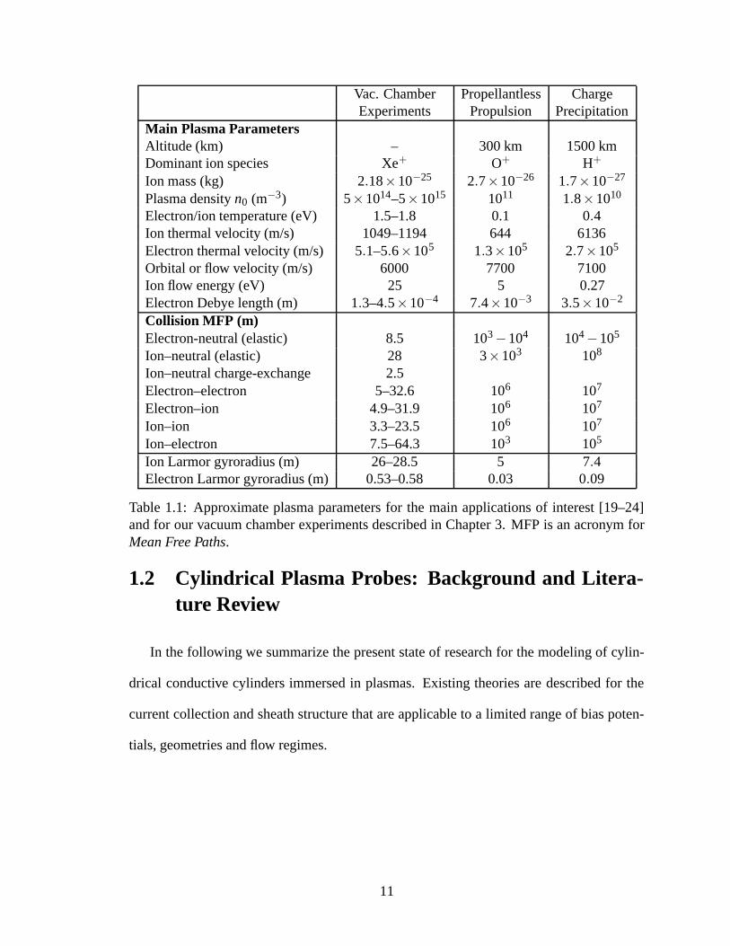
Table 1.1: Approximate plasma parameters for the main applications of interest [19–24]and for our vacuum chamber experiments described in Chapter 3. MFP is an acronym forMean Free Paths.
1.2 Cylindrical Plasma Probes: Background and Litera-ture Review
In the following we summarize the present state of research for the modeling of cylin-
drical conductive cylinders immersed in plasmas. Existing theories are described for the
current collection and sheath structure that are applicable to a limited range of bias poten-
tials, geometries and flow regimes.
11
1.2.1 Stationary plasmas
When considering the problem of a round cylindrical probe immersed in a stationary
plasma, there are two key parameters for the applications of interest:
• Current Collection (electron or ion current) is of concern in all three applications.
For propellantless propulsion, the tether bias potential is primarily positive, and we
seek to maximize electron current collection because it translates directly into avail-
able thrust. For charge precipitation, the tether is biased negatively, and we seek to
minimize the amount of ion current collected, because it translates into expended
power. In plasma diagnostics using Langmuir probes, expected current characteris-
tics as a function of plasma parameters must be precisely known in order to allow for
parameter extraction;
• Plasma sheath size and structure is a determining factor in the charge precipitation
application of electrostatic tethers. It determines the effective dimensions of the par-
ticle scatterer and thus its efficiency at precipitating high-energy electrons into the
loss cone [4].
The sheath structure and dimensions are closely linked to the particle kinetics, and can-
not be obtained by direct calculation for small and moderate-sized probes, even in the most
simple case of a round cylindrical probe in a stationary plasma. The Child Law sheath [25]
analytical expression, for example, is only applicable to probes with large dimensions as a
function of the Debye length, i.e., it is only valid in the thin-sheath limit, which is outside
of our regimes of interest.
Whereas sheath sizes cannot be computed directly for any probe size, exact analytical
expressions have been derived for the collected current to an attracting round conductive
cylinder immersed in a stationary, Maxwellian plasma. These expressions are only appli-
12

cable to two extreme regimes: the thin-sheath (infinite cylinder radius) and orbital-motion
(vanishing cylinder radius) limits. In the following, we provide a derivation of these limits.
1.2.1.1 Thin Sheath Limit
When the cylinder radius becomes sufficiently large, the current density collected to
the cylinder approaches that which would be collected on an infinite plate: this is the thin-
sheath limit.
Let us assume that an infinite plate, normal to the x axis, is the rightmost bound of
a 2-species Maxwellian plasma, with the velocity distribution functions of either plasma
species given by
fe,i (vx,vy) =n0me,i
2πeTe,iexp
{−
me,i
2eTe,i
(v2
x+ v2y
)}, (1.1)
where n0 is the background plasma number density in m−3, me,i is the electron or ion mass
in kg, Te,i is the electron or ion temperature in eV, and the velocity components vx and vy
are in m/s. First, note that the background density n0 is recovered by simply integrating
over velocity space:
ne,i =∫ +∞
vx=−∞
∫ +∞
vy=−∞fe,i (vx,vy)dvxdvy = n0. (1.2)
Now, let us assume that the infinite plate is biased at a potential V0 with respect to the
plasma potential (i.e., Vplate−Vplasma =V0). For either population (electrons and ions), the
current density collected on the infinite plate can be obtained by integrating the accelerated
or decelerated particle flux over all rightward-directed velocities on the plate’s left-side
surface, i.e.
Je,i = qe,iΓe,i
= qe,in0me,i
2πeTe,i×
+∞∫vx=
√max
(0,−
2qe,iV0me,i
)vy=+∞∫
vy=−∞
vx exp
{−
me,i
2eTe,i
[(v2
x+2qe,iV0
me,i
)+ v2
y
]}dvxdvy.
(1.3)
13

Performing the integral over vy, we get
Je,i = qe,in0
√me,i
2πeTe,i
+∞∫vx=
√max
(0,−
2qe,iV0me,i
) vx exp
{−
me,i
2eTe,i
(v2
x+2qe,iV0
me,i
)}dvx. (1.4)
Finally, we integrate over vx and obtain
Je,i = qe,in0
√eTe,i
2πme,i︸ ︷︷ ︸Jth
×
{1 qe,iV0 ≤ 0,
exp{−
qe,iV0eTe,i
}qe,iV0 > 0.
(1.5)
In Equation (1.5), Jth is simply the thermal current density, i.e., the average random current
density one finds at any location within the background plasma. This result shows that the
current density varies exponentially under a repelling bias and saturates to a constant value,
the thermal current Jth, for an attracting bias. The reason why the current density is limited
to the thermal current is that the sheath only extends in a single dimension, which precludes
any particle focusing.
1.2.1.2 Orbital-Motion Limit (“Thick” Sheath Limit)
We now consider the opposite limit, corresponding to a vanishing cylinder radius. In
practice, this limit is achieved when the cylinder radius falls below the Debye length. An
analytical expression for the OML current was first derived by Mott–Smith and Lang-
muir [26], based on conservation of energy and angular momentum in a central force
field. The orbital-motion-limit (OML) regime is attained when the cylinder radius is small
enough that all particle trajectories terminated on the cylinder’s surface are connected to
the background plasma, regardless of their angular momentum (i.e., none are connected to
another location on the probe’s surface). Since, in a collisionless plasma, the distribution
function is conserved along particle orbits, having all “directions of arrival” populated cor-
responds to an upper limit on the collected current. In the following, we derive the OML
current based on the precedent argument, similar to the approach used by Laframboise [6].
14
Using the alternative, but equivalent representation of velocity space in the form of
kinetic energy κ = me,i(v2x+v2
y)2eTe,i
in units of electron-volts and angular direction α in units of
radians, the energy distribution function of any given species at the surface of the probe
may be written:
ge,i (κ,α) =
{n0
2πTe,iexp
{−
eκ+qe,iVeTe,i
}κ >max(0,−qe,i
e V )
0 κ ≤max(0,−qe,ie V )
, (1.6)
where V is the local electric potential. The number density ne,i at the probe’s surface is
recovered by simply integrating over all of kinetic energy space and half of the angular
directions (since the probe blocks half of velocity space):
ne,i =
+∞∫κ=0
α=α ′+ 3π2∫
α=α ′+π/2
ge,i (κ,α)dκdα
=12
n0
{exp
(−
qe,iVeTe,i
), qe,iV ≤ 0
1, qe,iV > 0,
(1.7)
where α ′ is the angle between the outward surface normal and the x axis. Likewise, the
OML current density can be obtained by integrating the normal flux to the surface:
Je,i = qe,iΓe,i
= qe,i
+∞∫κ=0
α=α ′+ 3π2∫
α=α ′+π/2
√2eκme,i
cos(α−α ′
)︸ ︷︷ ︸
v⊥
fe,i (κ,α)dκdα
= qe,in0
√eTe,i
2πme,i︸ ︷︷ ︸Jthe,i
⎧⎨⎩
2√π
√−
qe,iVeTe,i+ exp
(−
qe,iVeTe,i
)erfc
(√−
qe,iVeTe,i
), qe,iV ≤ 0
exp(−
qe,iVeTe,i
), qe,iV > 0
.
(1.8)
Jth is the thermal current density and the complementary error function erfc(x) is given
by erfc(x) = 2√π∫ ∞
x e−t2dt. The repelled-species current is the same in the thin sheath and
OML limits, as can be seen by comparing (1.5) and (1.8) — this is called the retardation
region of the current characteristic and is valid in all regimes. The attracted-species current
is constant and equal to the thermal current in the thin-sheath limit, whereas in the OML
15
−10 −5 0 5 100
0.5
1
1.5
2
2.5
3
3.5
4
−qV/eT
I ts/I th
Thin−Sheath Saturation Region
Retardation Region
(a) Thin Sheath Normalized Current Character-istic (Eq. 1.5)
−10 −5 0 5 100
0.5
1
1.5
2
2.5
3
3.5
4
−qV/eT
I oml/I th
Retardation Region
OML SaturationRegion
(b) OML Normalized Current Characteristic(Eq. 1.8)
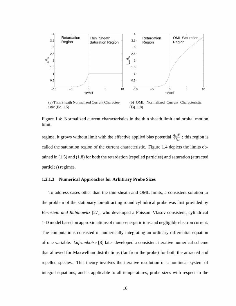
Figure 1.4: Normalized current characteristics in the thin sheath limit and orbital motionlimit.
regime, it grows without limit with the effective applied bias potential qe,iVeTe,i
; this region is
called the saturation region of the current characteristic. Figure 1.4 depicts the limits ob-
tained in (1.5) and (1.8) for both the retardation (repelled particles) and saturation (attracted
particles) regimes.
1.2.1.3 Numerical Approaches for Arbitrary Probe Sizes
To address cases other than the thin-sheath and OML limits, a consistent solution to
the problem of the stationary ion-attracting round cylindrical probe was first provided by
Bernstein and Rabinowitz [27], who developed a Poisson–Vlasov consistent, cylindrical
1-D model based on approximations of mono-energetic ions and negligible electron current.
The computations consisted of numerically integrating an ordinary differential equation
of one variable. Laframboise [8] later developed a consistent iterative numerical scheme
that allowed for Maxwellian distributions (far from the probe) for both the attracted and
repelled species. This theory involves the iterative resolution of a nonlinear system of
integral equations, and is applicable to all temperatures, probe sizes with respect to the
16

Debye length and potential values, although results were only given for relatively small
bias potentials.
In addition to providing results for the current collected to round cylindrical probes of
arbitrary sizes, these numerical schemes were the first to provide self-consistent results for
the density profiles of the attracted and repelled species.
1.2.2 Flowing Plasmas
1.2.2.1 Treatments Based on a Symmetric Potential Profile Assumption
Several authors have addressed, in a first-order sense, the problem of ion collection by
a round cylindrical probe immersed in a flowing plasma, using the crucial assumption of a
radially symmetric potential profile unaffected by any flow effects. Mott–Smith and Lang-
muir [26] derived an asymptotic formula valid in the limit of large speed ratios (relative to
the ion thermal velocity) for the current characteristic in the large-sheath limit (orbital mo-
tion limit). Kanal [28] derived similar expressions valid in the limit of small speed ratios.
Hoegy and Wharton [29] generalized those results by providing expressions valid for all
speed ratios, for the limiting cases of thin-sheath, large-sheath (orbital-motion-limit), and
retarding regimes.
Godard and Laframboise [30] went further by developing a numerical model that al-
lowed for all probe radii to be considered in the flowing case by using the 1-D cylindrically
symmetric potential profiles obtained by Laframboise [8] as the assumed electric potential.
In the case of the mesosonic regime, where the velocity of the flow is much larger
than the ion thermal velocity but much smaller than the electron thermal velocity, only
ion collection can be addressed by an approximate solution based on an assumed symmet-
ric potential profile. Such an approximation would show virtually no departure from the
stationary results in the case of electron collection, due to their large thermal velocity as
compared to the speed of the flow for the regimes of interest here. The effects of the flow
17

on the collection of the light species — the electrons— are thus only indirect. That is, these
effects only occur due to the asymmetries in the potential profile around the probe that are
induced by the heavier ion species. However indirect, these effects can be significant, as
will be seen in Chapter 4.
Even for the ion-attracting case, the assumption of a symmetric profile could fail to
provide a correct answer at least in cases showing one or more of these two conditions [30]:
• the probe radius is not small with respect to the Debye length, implying a non negli-
gible and likely asymmetric ion space-charge distribution near the collector;
• the ratio of flow energy to bias potential is neither very small (a small flow could
only cause small asymmetries) nor very large (in which case the bias potential could
not significantly affect the flow).
1.2.2.2 Consistent Numerical Treatments
A few numerical treatments have been performed to consistently model flow effects
on the sheath structure (i.e., asymmetries) and current collection to a round cylinder. In
the following we discuss some of the work that has been done using steady-state kinetic
approaches or particle-in-cell implementations.
1.2.2.2.1 Steady-State Kinetic Treatments Xu [17] and McMahon [22] have worked
on consistent steady-state kinetic models to address the problem of ion collection to a round
cylinder in a flowing plasma. The main difference between their approaches is that Xu uses
an inside-out trajectory tracking procedure whereas McMahon uses an outside-in strategy.
The outside-in steady-state method used by McMahon [22] bears some similarity with
the popular particle-in-cell plasma modeling techniques [25], in part due to the manner
in which the discrete charges are assigned to a fixed set of grid nodes. This approach is
18
intrinsically more efficient computationally, at the expense of some added numerical noise
associated with the charge assignment.
The inside-out approach used by Xu [17] and in the present work, although not as
efficient computationally, is based on a direct sampling of the velocity distribution function
at the nodes of a mesh.
1.2.2.2.2 Particle-in-Cell Treatment Onishi [31] has performed simulations of a single
electron-attracting cylinder immersed in a flowing unmagnetized plasma using a particle-
in-cell approach. His findings indicate that a population of trapped electrons, upstream
of the cylinder, is necessary for the plasma to reach a steady state. This requirement is
attributed to the fact that the local increase of the ion density on the ram side of the cylinder,
beyond the ambient density, must be matched by an increased electron density to satisfy
the quasi-neutrality condition. Limitations on the computational zone size may be in part
responsible for this computational requirement, and it is not clear whether or not this is a
physical requirement.
1.3 Summary of Research Contributions
The general aim of the research that has led to this thesis was to improve the understand-
ing of the steady-state perturbations caused in a two-species plasma (flowing or stationary)
by the introduction of a long conductive cylinder (e.g., an electrodynamic tether) of arbi-
trary cross-section geometry, biased at a specified potential. Specifically, our main interests
were to determine
• the structure of the plasma sheath/pre-sheath, and
• the amount of collected current
19

as a function of cylinder geometry, bias potential, and plasma flow speed. These objectives
have required both the development of a new computer model capable of accurately sim-
ulating the general problem of interest, and an experimental investigation using a vacuum
chamber. Consequently, the contributions of the research presented in this thesis fall in one
of three major categories:
1. a computational model for the self-consistent modeling of arbitrary 2-D conductive
structures immersed in flowing plasmas;
2. new computer simulation results for regimes (combination of biases, geometries, and
plasma flow) not addressed in previous research;
3. new experimental results pertaining to the effects of plasma flow and geometry on
electron collection.
We describe these contributions in more detail in the following three sub-sections corre-
sponding to the three major categories outlined above.
1.3.1 A Self-Consistent Steady-State Kinetic Model for Arbitrary 2-DConductive Structures in Flowing Plasmas
A new computational model was created for the self-consistent kinetic modeling of the
charge-imbalance structure forming around arbitrary two-dimensional conductive objects
immersed in stationary and flowing two-species plasmas. The following are some new
contributions brought about by this new model.
1. A dynamic, adaptive, unstructured meshing strategy that allows support for arbitrary
2-D geometries and can accurately resolve features with widely disparate scales, such
as very small probes together with very large sheath structures. Another typical
plasma feature that requires this dynamic resolution capability is the narrow surge
20

of the net charge density found at the sheath edge (a location not known a priori) in
the case of high-voltage biases, which is attributed to the combination of the density
profiles of the counter-streaming attracted and repelled species.
2. A new approach based on a Tikhonov-regularized Newton method for the efficient
minimization of the nonlinear least-squares problem, which provides a numerical
approximation for the fixed point of the Poisson–Vlasov operator. This approach is
robust to numerical instabilities and numerical noise as well as very versatile, in that
it can successfully solve a wide class of 2-D problems without the need for empirical
tuning of parameters such as is required by overrelaxation techniques [17].
3. Support for the kinetic treatment of both ions and electrons, even in the case of a
flowing plasma. Previous treatments of the flowing plasma case, applied for ion
collection only, have assumed “Boltzmann” electrons [17, 22].
4. A parallel implementation of the 2-D Vlasov solver based on the PVM library [32],
which enables a very accurate representation of plasmas extending over large do-
mains within reasonable computing times. The parallel code is a coarse-grained
MPMD (Multiple Processors, Multiple Data) implementation that runs efficiently on
a dynamically-configured scattered network of workstations, using their idle com-
puting time. The code was developed and tested on scattered networks of Sun™
and Linux workstations, and also has been tested successfully on a standard Linux
cluster.
1.3.2 New Simulation Results
Using this new steady-state kinetic model, a collection of new results applicable to
the problems of interest have been obtained via computer simulation. These new results
21

provide:
1. an extension of the operating regimes covered by Laframboise [8], Xu [17] and
McMahon [22] to a wider range of bias potentials. Bias potentials from an arbitrary
small fraction of the plasma temperature T up to 10,000T have been successfully
covered by the cylindrical 1-D model. The full 2-D model has reached 640Te.
2. an assessment of wire interference effects on sheath structure and current collection
based on two parallel round cylinders with various center-to-center spacings in a
stationary plasma.
3. an assesment of the sheath structure and current collection for the case of a thin tape
cylinder.
4. an assessment of plasma flow effects on sheath structure and current collection for
both ion- and electron-attracting round cylinders. The electron-collecting case has
not been previously successfully analyzed in an unmagnetized plasma.2 As for the
ion-collecting case, it has previously been addressed by Xu [17] and McMahon [22]
using a Boltzmann approximation for the electrons. The present research contains the
first results of simulations using a non-PIC fully kinetic treatment for both species in
a flowing plasma.
To the author’s knowledge, items 2 and 3 constitute the first fully self-consistent kinetic
simulation results for cylinder geometries other than circular cylinders.
1.3.3 New Experimental Results
Experimental testing of electron collection to tether samples of various geometries in
a mesosonic xenon plasma were performed using the Large Vacuum Test Facility at the
2Onishi [31] has reported that his particle-in-cell code could not reach a steady state when simulating aflowing, collisionless, unmagnetized plasma.
22

University of Michigan’s Plasmadynamics and Electric Propulsion Laboratory. New ex-
perimental results were obtained pertaining to
• the effect of plasma flow on the electron collection to round cylinders (a significant
enhancement was observed); and
• a comparison of electron current collection efficiencies of solid and slotted tape tether
samples, oriented parallel and perpendicular to plasma flow.
The geometry effects observed during these experiments are in general agreement with
those predicted by our kinetic model. As for the electron current enhancement associated
with the mesosonic plasma flow, it cannot be predicted by our collisionless plasma model.
However, the sheath structures obtained via simulation give some indication as to how
pre-sheath collisions may have caused the observed enhancement.
1.4 Dissertation Overview
The five chapters of this dissertation are structured as follows:
Chapter 1 provides motivation, defines the problem of interest, reviews previous relevant
research, and summarizes research contributions.
Chapter 2 develops the theory and describes the computer implementation of a steady-
state Poisson–Vlasov self-consistent computational model based on kinetic theory.
The model is applicable to a wide range of 2-D objects immersed in stationary and
flowing plasmas. Both a 1-D cylindrical implementation and a full 2-D implementa-
tion are presented side-by-side.
Chapter 3 describes the experimental testing of electron-collecting tether samples in a
mesosonic flowing plasma. The sample geometries tested include a round cylinder,
thin solid tapes, and thin slotted tapes.
23

Chapter 4 presents and discusses the results and analyses of the kinetic simulations per-
formed using the computer model defined in Chapter 2. Comparisons with our ex-
perimental results are also shown.
Chapter 5 discusses the conclusions of this dissertation and provides suggestions for fu-
ture research.
24

CHAPTER 2
Steady-State Poisson–Vlasov Model: Theory andImplementation
We present the theory and software implementation of a consistent, steady-state, elec-
trodynamic plasma model based on kinetic theory. The solver presented here is best clas-
sified as a Vlasov code based on a kinetic description of plasmas [33]. It differs from
particle-in-cell methods in that the Vlasov equation is solved directly instead of resorting
to a set of discrete macro-particles. It is also distinct from Eulerian Vlasov implemen-
tations [34], owing primarily to the fact that a steady-state “non time-varying” solution is
sought directly, without resorting to incremental time stepping. The steady-state solver pre-
sented here bears some similarity with previous work addressing other geometries [35–37],
and may be regarded as a 2-D extension of the 1-D cylindrical model developed by Lafram-
boise [8].
The general aim of this model is to numerically solve, in a self-consistent manner, the
Poisson and Vlasov equations in a steady state over a large computational region around an
arbitrarily-shaped 2-D conductive body in a collisionless, unmagnetized, flowing 2-species
plasma. The implementation of the 2-D solver, called KiPS-2D (Kinetic Plasma Solver,
2-dimensional) consists of successive linearizations of the nonlinear Poisson–Vlasov op-
erator, within a Tikhonov-regularized Newton iterative process. Following are listed the
main features of the proposed model and solver:
25

• it allows for the representation of the complete, arbitrary velocity distribution of both
plasma species at all sampled locations in the computational domain;
• it can model plasma cross flow in all speed regimes with respect to the ion thermal
velocity;
• it includes a finite-element-based Poisson solver incorporating a background plasma
boundary condition based on asymptotic analytical results [27];
• it provides a dynamic, adaptive, unstructured meshing strategy, allowing for the res-
olution of sheath asymmetries induced by the plasma flow and the support of con-
ductive objects with arbitrary 2-D geometries;
• it allows for the simulation of very large computational domains in order to accom-
modate the pronounced pre-sheath elongation along the direction of plasma flow. The
variable grid size is tailored locally to efficiently accommodate potential variations.
Numerical instabilities resulting from large grid sizes are handled using a Tikhonov
regularization process;
• its steady-state Vlasov solver features a parallel implementation based on the PVM
library [32], allowing it to run on either a single host, a parallel architecture, or a
scattered network of workstations based on a MPMD (Multiple Processors, Multiple
Data) scheme.
Although the primary purpose of this work was to provide a 2-D solver, a 1-D cylin-
drical implementation of this model, called KiPS-1D, was also developed. This 1-D code
has been validated against results from Laframboise [8], and extends the covered range of
probe bias potentials from 25Te to 10,000Te. In addition, it serves as a validation tool for
the 2-D implementation of the code. In the following sections, the general formulation will
26

be described consistent with the 2-D implementation. However, where necessary, specific
derivations will be presented pertaining to the 1-D and 2-D implementations of each com-
ponent. Note that the main symbols used throughout this chapter and others are listed in
Appendix A for convenience.
2.1 Basic Assumptions
The aim of the steady-state, consistent kinetic plasma model presented in this thesis is
to provide an accurate representation of the dominant physical mechanisms involved in the
formation of a steady-state sheath as well as in current collection to 2-D conductive bodies.
In setting up the basic physics underlying the model, we make the following assumptions
regarding the physical mechanisms involved in the sheath–plasma system:
• the plasma is collisionless;
• a steady state exists;
• the plasma is unmagnetized;
• the background plasma is a drifting Maxwellian;
• end effects are negligible;and
• trapped orbits are unpopulated.
Let us now describe in more detail each of these assumptions.
The Plasma is Collisionless Several types of collisions can be considered. Based on the
very long mean free paths given in Table 1.1, we can certainly neglect the elastic
ion–neutral and electron–neutral collisions for all three cases (vacuum chamber ex-
periment, electrodynamic tethers, and electrostatic tethers), because they are much
larger than the typical sheath sizes we are interested in.
27

Coulomb collisions are also neglected, i.e., we assume that the forces experienced
by any of the charged particles forming the plasma are entirely due to the collective
effect of the charge density contributed by all particles, not to their individual ef-
fect. This assumption is accurate for sufficiently low plasma densities (such as space
plasmas), in which any given particle very rarely “meets” another particle in a close
encounter. In other words, the number of particles contained within the “sphere of
influence” (Debye sphere) of a given particle is so large that the overall forces are
overwhelmingly attributable to the bulk of the plasma.
A Steady State Exists We assume that there exists a steady state of the plasma density and
potential distributions in the frame of reference of the moving tether or probe. By
“steady state” we imply a state in which there are no time variations of the plasma
density or electric potential anywhere in the frame of reference of the moving object.
Our definition of the steady state allows for a steady flow of plasma particles in any
directions where applicable, including a net drift component of the plasma bulk due
to the orbital motion of the tether. This implies that time variations may be perceived
as seen from other frames of reference.
The existence of a steady state will be proved a posteriori by showing that we can
find a self-consistent, steady-state solution satisfying both the steady-state Vlasov
and Poisson equations. Proving the existence of a steady state is not, however, a
guarantee that no time variations can exist even in the absence of transients and ex-
ternal excitations. Nonetheless, the steady-state solution that we provide here can be
regarded as a lowest energy state that the electrodynamic forces will seek to attain in
order to minimize the system energy.
The Plasma is Unmagnetized We assume that the effect of the magnetic field on the so-
28

lution is negligible, and therefore choose to neglect the magnetic field force in our
computational model. To qualify this approximation, let us consider the effect of
the magnetic field for the main applications of interest. This effect can be gaged by
comparing the typical gyroradius of the attracted species within the computational
domain to the size of the computational zone, which is typically on the order of the
sheath dimensions. The effect of the magnetic field on the repelled species’ density
is unimportant as long as the said species does not have a sizable drift component
as compared to its thermal distribution, because then the local densities are solely
determined by the local potential for all practical purposes. This applies to the elec-
trons when using a negative bias potential, since their drift velocity is negligible in
the regimes of interest.
For charge precipitation, the magnetic field effect on the repelled electrons is there-
fore negligible for the reason just mentioned. As for the attracted ions, Table 1.1 lists
for their gyroradius in the background plasma a value of 7.4 m, which is admittedly
smaller than the typical sheath diameters of interest for tether bias potentials in the
vicinity of 100,000 volts. However, this relatively small value of the Larmor gyrora-
dius should be put into perspective, because it only applies in the background plasma
where particle velocities are on the order of the thermal velocity. Within the acceler-
ating potential of the sheath structure however, the attracted particles are accelerated
to velocities that can be up to a few hundred times the thermal velocities, for tether
bias potentials of a few tens of thousands of volts. The gyroradius rG is proportional
to the ratio of the particle velocity to the magnetic field intensity [38],
rG =miveB, (2.1)
where the magnetic field B is in units of Tesla and v is the local ion velocity. Inside the
sheath the accelerated species’ gyroradius scales proportional to particle velocities,
29

to values much larger than the corresponding sheath size. For example, consider a
one-Debye-length-radius ion-attracting tether, used for charge precipitation, biased
at 100,000 volts. Scaling the ion Larmor gyroradius proportional to the ratio of in-
sheath velocity to the thermal velocity, the ion gyroradius close to the probe is given
by
rG ≈
√100000eV
0.4eVrGL
∣∣∣∣∣rGL=7.4 m
=√
250000×7.4 m= 3700 m. (2.2)
This result is significantly larger than any practical sheath size, and emphasizes the
fact that the magnetic field should not play a significant role in this application. For
this specific bias potential and a tether radius of one Debye length, the sheath diame-
ter is about 92 meters according to the asymptotic expressions derived in Chapter 4.
For propellantless propulsion applications, the electrons are the attracted species.
Their relatively small Larmor gyroradius of 3 cm would be scaled up, within a sheath
created by a typical 1 kV-biased tether, to a value of
rG ≈
√10000.1
rGL
∣∣∣∣∣rGL=0.03 m
=√
10000×0.03 m= 3 m, (2.3)
which is also significantly larger than the approximate sheath diameter of 0.5 m.
In general, we can therefore say that attracted species can be expected to have large
gyroradii for most of the sheath as compared to the sheath’s dimensions. This means
that the magnetic field is playing a relatively minor role in the sheath formation and
current collection processes, and may thus be safely ignored for these purposes, es-
pecially for the charge precipitation application where bias voltages are typically
larger than in the propulsion application. A similar reasoning can be made based on
a comparison of the magnitudes of the electrostatic and magnetic forces acting on the
particles: the electrostatic field forces can be as much as a few orders of magnitude
larger than the magnetic field forces.
30

Our kinetic model therefore assumes that no magnetic fields are present, resulting in
a purely electrostatic solution of the plasma sheath.
The Background Plasma is a Drifting Maxwellian Although no assumptions are made
with regards to the velocity distributions within the computational domain, the source
of the plasma entering the computational domain must be known and is defined as a
boundary condition. The computational domain must be made sufficiently large to
include all of the major perturbations on the plasma caused by the presence of a con-
ductive object. The velocity distribution of the incoming plasma particles entering
the simulation domain is thus assumed to closely correspond to the ambient veloc-
ity distribution that exists in the background (undisturbed) plasma. In a stationary
plasma, the 2-D velocity distribution is assumed to be Maxwellian (see equation 1.1).
For a moving plasma, the background velocity distribution function for both electron
and ion species becomes
fe,i (vx,vy) =n0me,i
2πeTe,iexp
{−
me,i
2eTe,i
[(vx−U)2+ v2
y
]}, (2.4)
where we assume that the plasma is moving along the direction of the x axis with
velocity U . Note that the vz dependence of the 3-D velocity distribution function
has been integrated out into a constant in front of equations (1.1) and (2.4) since
we only consider 2-D structures in unmagnetized plasma, which implies that the vz
Maxwellian dependence of the plasma is unchanged throughout the computational
domain. Section 2.4.2.2 provides more detail regarding the method used to account
for the small perturbations to this distribution function that occur between the back-
ground plasma (at r→ ∞) and the outer boundary of the computational domain.
End Effects are Negligible Probe end effects are neglected in this treatment. This is
hardly an approximation in the case of bare, space borne electrodynamic tethers,
31

which are typically several kilometers long, corresponding to lengths of tens of thou-
sands of Debye lengths and beyond. In the case of laboratory probes of more modest
lengths, the end effect can be neglected provided that the cylinder is of sufficient
length. The typical probes considered here are several hundred to a few thousand
Debye lengths long. In addition, it has been shown, at least for ion-attracting probes,
that end effects are negligible provided that the probe is oriented perpendicular to the
direction of plasma flow. [39]
Trapped Orbits are Unpopulated In our analysis, we assume that trapped particle or-
bits are unpopulated, which is consistent with the treatments described by Lafram-
boise [8] and Xu [17] (more detail is given in Section 2.4). This assumption fol-
lows from the previous “collisionless” and “steady-state” assumptions. When both
of these assumptions hold, all particles present anywhere in the vicinity of the 2-D
object can be traced back to the background plasma (the “source”) on collisionless
orbits. Therefore closed orbits cannot be populated because they have no source.
Collisions, when they occur, may be regarded as scattering events that can displace
a particle from one “collisionless orbit” to another. The present assumption, based
on a “conservation of orbits” argument, is appropriate for the plasmas of interest (see
Table 1.1), because they feature very few collisions, implying that the “paths” con-
necting two points in the background plasma or connecting the background plasma
to the tether can be traversed by a particle with virtually no collision events. Time
variations, which could be induced by external perturbations such as variations in the
plasma environment, can also be regarded as scattering events, similar to collisions.
The present treatment does not account for any “filling” of the trapped orbits that
could result from such time variations. The impact of collisional and time-varying
effects on the level of filling of trapped orbits will be assessed as part of future re-
32
search. Some authors have provided indications as to how this may be done [40,41].
As pointed out by Prof.Laframboise3 in recent discussions, trapped orbits could also
potentially be filled by some of the particles entering through the ends of the cylindri-
cal sheath of a tether, since some of the so-called “trapped“ collisionless orbits may
actually be connected to the background plasma through the hemispherical end caps
of the long, but finite, cylindrical sheath enclosing the tether. The level of “steady-
state filling” of trapped orbits attained through this mechanism should be assessed as
part of future research but is beyond the scope of the present work.
2.2 Poisson–Vlasov Representation of Collisionless Plas-mas
Obtaining a simultaneous solution in two dimensions for the asymmetric steady-state
electric potential distribution and charge density distributions of both plasma species (ions
and electrons) requires the ability to solve, self-consistently, Vlasov’s equation for each
species and Poisson’s equation for the electric potential and charges, while satisfying ap-
propriate boundary conditions.
Both the electric potential and charge densities are sampled on a piecewise-triangular
mesh, which is generated using the Bidimensional Anisotropic Mesh Generator (BAMG)
developed at INRIA, France [42]. An adaptive process was implemented whereby the
BAMG mesher is used to periodically refine the mesh based on the best available approxi-
mation of the net charge density and potential distributions.
In charged media such as a plasma, the steady state of the potential distribution and net
charge distribution obeys Poisson’s equation [43],
∇2V (x,y) =−ρ(x,y)
ε0, (2.5)
3Prof. James G. Laframboise, York University, Ontario, Canada.
33

at any point within the plasma. In addition, each species comprising the plasma, that is,
electrons and ions, is composed of particles with a distribution of velocities at any point
in space f3d (x,y,z,vx,vy,vz). In an unmagnetized electrostatic plasma bounded with 2-
dimensional boundaries, the distribution of velocities along the third dimension is inde-
pendent of position, such that we only need to keep track of the 2-dimensional velocity
distribution function obtained by integrating along vz
f2d (x,y,vx,vy) =
vz=+∞∫vz=−∞
dvz f3d (x,y,vx,vy,vz) , (2.6)
where the z variable was dropped because the 2-D boundary conditions preclude any de-
pendence on z. The number density of each species is obtained by integrating the velocity
distribution function over all velocity space,
ne,i =
∫ ∫fe,i(x,y,vx,vy) dvxdvy, (2.7)
where the indices e and i refer to electrons and ions, respectively. The net charge density
results from
ρ(x,y) = qini(x,y)+qene(x,y), (2.8)
where qe and qi are the electron and ion particle charge.
In a collisionless, unmagnetized plasma at the steady state, the velocity distribution
functions f (x,y,vx,vy) of each species is conserved along particle orbits. This is stated by
Vlasov’s equation in the steady state (∂ f∂ t= 0) [25],
d fe,i
dt= vx
∂ fe,i
∂x+ vy
∂ fe,i
∂y−
qe,i
me,i
∂V∂x
∂ fe,i
∂vx−
qe,i
me,i
∂V∂y
∂ fe,i
∂vy= 0, (2.9)
where we substituted the electric field components with the gradient of the electric poten-
tial, i.e., �E =−∇V . Given a known potential distribution and a boundary condition for the
incoming particles at the outer boundary of the computational domain, the method of char-
acteristics can be used to solve (2.9) for the velocity distributions fe,i(x,y,vx,vy) of both the
electrons and ions, at all positions and for all velocities.
34
The use of the method of characteristics for the resolution of Vlasov’s equation in
plasma problems was reported early on [36], and was referred to as the inside-out proce-
dure. It consists of tracking a particle’s trajectory back in time until it intersects the “source
boundary” (which in our case is the outer boundary) of computational space, where the ve-
locity distribution function is sampled. Any trajectory not originating from the outer shell
is deemed unpopulated [8]. Such is the case for trajectories originating from the tether
itself, which we assume does not emit charged particles, as well as trapped trajectories,
which have no sources in the collisionless case.
The steady-state of the plasma must simultaneously satisfy Poisson’s equation (2.5) and
Vlasov’s equation (2.9), subject to boundary conditions on the potential and the incoming
particles. To find the steady-state solution, both a Poisson and a Vlasov operator are needed:
• the Poisson operator solves for the potential distribution V (x,y), given a net charge
distribution ρ(x,y) together with boundary conditions on the potential distribution,
consistent with Poisson’s equation (2.5);
• the Vlasov operator solves for the charge distribution ρ(x,y), given a potential distri-
bution V (x,y), consistent with Vlasov’s equation equation (2.9) as well as equations
(2.7) and (2.8).
Let the Poisson operator be defined by the functional
fP : V (x,y) = fP {ρin(x,y)} , (2.10)
and the Vlasov operator be defined by the functional
fV : ρout(x,y) = fV {V (x,y)} . (2.11)
Then the solution of the problem lies at the fixed point of the Poisson–Vlasov functional,
35
defined as a composition of the Poisson and Vlasov functionals:
fPV : ρout(x,y) = fPV {ρin(x,y)}= fV { fP {ρin(x,y)}} . (2.12)
That is, the solution for the net charge distribution ρ(x,y) is that which, when given at the
input of the Poisson–Vlasov operator, yields an identical output (ρout(x,y) = ρin(x,y)). A
Vlasov-Poisson operator could also be considered that would have V (x,y) as its input and
output. The Poisson–Vlasov operator was chosen because of a stability advantage inherent
to the regularization process discussed later.
In the following, we present the specific Poisson and Vlasov solvers used in both our
1-D and 2-D implementations. We then proceed to define an algorithm for finding a best
approximation to the fixed point of the Poisson–Vlasov operator, i.e., the steady state of the
plasma.
2.3 Finite-Element Poisson Solver
Here we derive the Poisson solver, a numerical approximation for the Poisson operator
defined above by the functional fP. The Poisson solver will provide the capability to obtain
a numerical approximation for the potential distribution satisfying Poisson’s equation and
boundary conditions for a given net charge density distribution. We have chosen to use
the finite-element method to implement our Poisson solver, due to its relative simplicity
and mathematical compactness. In addition, it does not present any of the numerical issues
associated with the poles generated with techniques such as the method of moments.
The approximate character of the Poisson solver is due to the finite discretization em-
ployed to solve Poisson’s differential equation (2.5). Both the potential and charge distri-
butions are assumed piecewise-linear, and the accuracy of this representation improves as
the mesh density increases.
In the following, we show two separate derivations for the 1-D cylindrical Poisson
36

Solver, used in KiPS-1D, and for the full 2-D Poisson Solver, used in KiPS-2D.
2.3.1 1-D Cylindrical Implementation
In the absence of any azimuthal variation of either the charge distribution or boundary
conditions on the potential, Poisson’s equation (2.5) simplifies to
1r
ddr
(r
dVdr
)=−
1ε0
ρ (r) . (2.13)
Finding a unique solution for this differential equation requires boundary conditions on
V (r). At the surface of the probe, located at r= r0, we require that the potential be equal to
the applied bias voltage, i.e., V (r = r0) =V0. Now, our computational domain is finite and
terminates at a large radius r = rM. We have found that the most suitable boundary condi-
tion to represent an open-ended plasma domain is a floating boundary condition based on
the asymptotic potential profile V (r) ∝ 1/r derived by Bernstein and Rabinowitz [27] and
also used by Laframboise [8]. This asymptotic behavior, together with the bias potential,
results in the following boundary conditions for the potential:
V (r = r0) =V0, (2.14)
dVdr
∣∣∣∣r=rM
=−Vr
∣∣∣∣r=rM
. (2.15)
According to variational principles [44, 45], which are the foundation of the finite-
element method, the solution of (2.13), subject to boundary conditions defined in (2.14)–
(2.15), is equivalent to the stationary point (or minimum energy point) of the following
functional:
Π=∫ rM
r0
dr
[12
rV ′2(r)−rρ(r)V (r)
ε0
]+
V 2
2
∣∣∣∣r=rM
. (2.16)
37
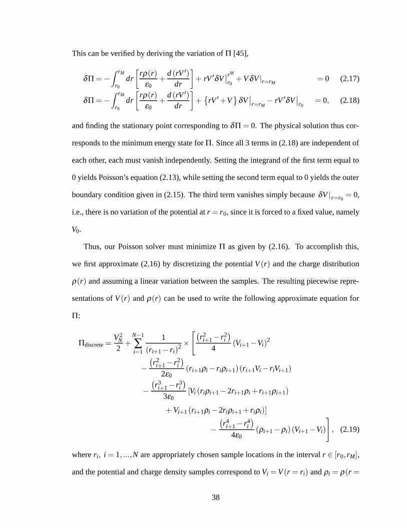
This can be verified by deriving the variation of Π [45],
δΠ=−∫ rM
r0
dr
[rρ(r)
ε0+
d (rV ′)dr
]+ rV ′δV
∣∣rM
r0+ V δV |r=rM
= 0 (2.17)
δΠ=−∫ rM
r0
dr
[rρ(r)
ε0+
d (rV ′)dr
]+{
rV ′+V}
δV∣∣r=rM− rV ′δV
∣∣r0
= 0, (2.18)
and finding the stationary point corresponding to δΠ = 0. The physical solution thus cor-
responds to the minimum energy state for Π. Since all 3 terms in (2.18) are independent of
each other, each must vanish independently. Setting the integrand of the first term equal to
0 yields Poisson’s equation (2.13), while setting the second term equal to 0 yields the outer
boundary condition given in (2.15). The third term vanishes simply because δV |r=r0= 0,
i.e., there is no variation of the potential at r= r0, since it is forced to a fixed value, namely
V0.
Thus, our Poisson solver must minimize Π as given by (2.16). To accomplish this,
we first approximate (2.16) by discretizing the potential V (r) and the charge distribution
ρ(r) and assuming a linear variation between the samples. The resulting piecewise repre-
sentations of V (r) and ρ(r) can be used to write the following approximate equation for
Π:
Πdiscrete =V 2
N
2+
N−1
∑i=1
1
(ri+1− ri)2 ×
[(r2
i+1− r2i
)4
(Vi+1−Vi)2
−
(r2
i+1− r2i
)2ε0
(ri+1ρi− riρi+1)(ri+1Vi− riVi+1)
−
(r3
i+1− r3i
)3ε0
[Vi (riρi+1−2ri+1ρi+ ri+1ρi+1)
+ Vi+1 (ri+1ρi−2riρi+1+ riρi)]
−
(r4
i+1− r4i
)4ε0
(ρi+1−ρi)(Vi+1−Vi)
], (2.19)
where ri, i= 1, ...,N are appropriately chosen sample locations in the interval r ∈ [r0,rM],
and the potential and charge density samples correspond to Vi =V (r = ri) and ρi = ρ(r =
38

ri). The equivalent matrix-form expression is:
Π≈Πdiscrete =12�V T KN×N�V −
1ε0
�V T QN×N�ρ, (2.20)
where K and Q are N×N matrices, and the elements of the vectors �V and �ρ correspond to
the potential and charge density samples Vi and ρi for i ∈ [1,N]. The non-zero elements of
matrix K are given by
1st row: K1,1 =r2
2− r21
2(r2− r1)2 , K1,2 =−
r22− r2
1
2(r2− r1)2
ith row: Ki,i−1 =r2
i−1− r2i
2(ri− ri−1)2 , Ki,i =
r2i − r2
i−1
2(ri− ri−1)2 +
r2i+1− r2
i
2(ri+1− ri)2
and Ki,i+1 =r2
i − r2i+1
2(ri+1− ri)2 , i ∈ [2,N−1]
Nth row: KN,N−1 =−r2
N− r2N−1
2(rN− rN−1)2 , KN,N = 1+
r2N− r2
N−1
2(rN− rN−1)2 .
(2.21)
With regards to matrix Q, the non-zero elements of its first row are given by
Q1,1 =1
(r2− r1)2
[12
r22
(r2
2− r21
)−
23
r2(r3
2− r31
)+
14
(r4
2− r41
)]and
Q1,2 =1
(r2− r1)2
[−
12
r1r2(r2
2− r21
)+
13(r1+ r2)
(r3
2− r31
)−
14
(r4
2− r41
)],
(2.22)
the non-zero elements of rows 2 through N−1 are given by
Qi,i−1 =1
(ri− ri−1)2
[−
12
ri−1ri(r2
i − r2i−1
)+
13(ri−1+ ri)
(r3
i − r3i−1
)−
14
(r4
i − r4i−1
)],
Qi,i =1
(ri− ri−1)2
[12
r2i−1
(r2
i − r2i−1
)−
23
ri−1(r3
i − r3i−1
)+
14
(r4
i − r4i−1
)]
+1
(ri+1− ri)2
[12
r2i+1
(r2
i+1− r2i
)−
23
ri+1(r3
i+1− r3i
)+
14
(r4
i+1− r4i
)], and
Qi,i+1 =1
(ri+1− ri)2
[−
12
riri+1(r2
i+1− r2i
)+
13(ri+ ri+1)
(r3
i+1− r3i
)−
14
(r4
i+1− r4i
)],
(2.23)
39

and the non-zero elements of its N th row are given by
QN,N−1 =1
(rN− rN−1)2
[−
12
rN−1rN(r2
N− r2N−1
)+
13(rN−1+ rN)
(r3
N− r3N−1
)−
14
(r4
N− r4N−1
)]and
QN,N =1
(rN− rN−1)2
[12
r2N−1
(r2
N− r2N−1
)−
23
rN−1(r3
N− r3N−1
)+
14
(r4
N− r4N−1
)],
(2.24)
with all the unspecified matrix elements equal to zero.
Now, the best approximation to the physical solution, i.e., the stationary point of Π,
which is also the root of δΠ as specified in (2.18), is obtained by setting to zero the partial
derivatives of Πdiscrete with respect to the unknown potential samples Vi, i = 2, ...,N. This
operation yields the following linear system of equations:
K2:N,2:N�V2:N =1ε0
Q2:N,1:N�ρ−V0K2:N,1. (2.25)
This system is then solved for the unknown potential samples Vi, i ∈ [2,N]:
�V2:N =
[1ε0(K2:N,2:N)
−1 Q2:N,1:N
]︸ ︷︷ ︸
JP′N−1×N
�ρ −V0 (K2:N,2:N)−1 K2:N,1︸ ︷︷ ︸
�V cst′
, (2.26)
where we have defined an (N−1)×N matrix JP′ and a vector�V cst′ with (N−1) elements.
Based on this result and the potential boundary condition at r = r0, we can form the com-
plete Poisson solver as follows:
�V = JP�ρ+�V cst, (2.27)
with
JP2:N,1:N = JP′, (2.28)
JP1,1:N =�0, (2.29)
�V cst2:N =�V
cst′, and (2.30)
V cst1 =V0. (2.31)
40
The expression given by (2.27) is the final compact form of our finite element-based cylin-
drical 1-D Poisson solver. It is obviously a linear operator, and only needs to be computed
once upon generating a new grid.
2.3.2 2-D Implementation
For the 2-D implementation of our Poisson solver, we wish to approximately solve, in
two dimensions, Poisson’s equation (2.5), with appropriate boundary conditions. We will
first focus on the boundary conditions, and then proceed to derive the finite element solver
itself.
2.3.2.1 Poisson Boundary Conditions
At the surface of the conductive object(s) (e.g., probe), we simply enforce a fixed bias
potential V =V0, with the potential V being measured from infinity.
The question of the outer boundary condition is significantly more difficult to address.
Since the computational domain must be finite, an appropriate outer boundary condition
should be selected that will help keep the required extent of the computational domain at a
reasonable size. In its undisturbed state, the plasma is neutral, and it therefore acts to shield
any perturbations in the electric potential caused by a biased conductive object inserted
within that plasma. For that reason, we can make the argument that the potential profile,
beyond the circular outer edge of the computational domain, must fall off faster than it
would in free space.
In free space, we drop the space charge term ρ(x,y) on the right-hand side of Pois-
son’s equation (eq. (2.5)), and recover Laplace’s equation. In 2-D cylindrical coordinates,
Laplace’s equation can be written as
∇2V =1r
∂∂ r
(r
∂V∂ r
)+
1r2
∂ 2V∂θ 2 = 0 (2.32)
41
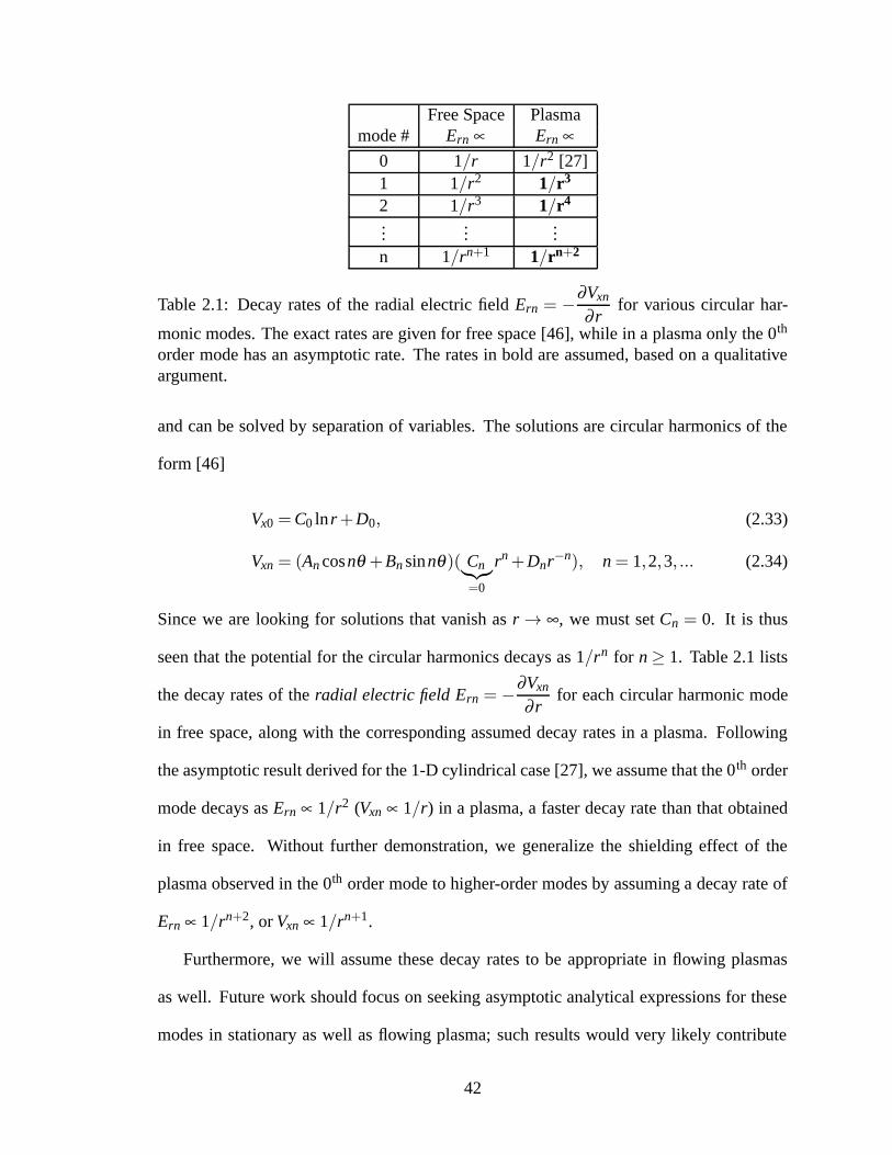
Free Space Plasmamode # Ern ∝ Ern ∝
0 1/r 1/r2 [27]1 1/r2 1/r3
2 1/r3 1/r4
......
...n 1/rn+1 1/rn+2
Table 2.1: Decay rates of the radial electric field Ern = −∂Vxn
∂ rfor various circular har-
monic modes. The exact rates are given for free space [46], while in a plasma only the 0th
order mode has an asymptotic rate. The rates in bold are assumed, based on a qualitativeargument.
and can be solved by separation of variables. The solutions are circular harmonics of the
form [46]
Vx0 =C0 lnr+D0, (2.33)
Vxn = (An cosnθ +Bn sinnθ)( Cn︸︷︷︸=0
rn+Dnr−n), n= 1,2,3, ... (2.34)
Since we are looking for solutions that vanish as r→ ∞, we must set Cn = 0. It is thus
seen that the potential for the circular harmonics decays as 1/rn for n≥ 1. Table 2.1 lists
the decay rates of the radial electric field Ern = −∂Vxn
∂ rfor each circular harmonic mode
in free space, along with the corresponding assumed decay rates in a plasma. Following
the asymptotic result derived for the 1-D cylindrical case [27], we assume that the 0th order
mode decays as Ern ∝ 1/r2 (Vxn ∝ 1/r) in a plasma, a faster decay rate than that obtained
in free space. Without further demonstration, we generalize the shielding effect of the
plasma observed in the 0th order mode to higher-order modes by assuming a decay rate of
Ern ∝ 1/rn+2, or Vxn ∝ 1/rn+1.
Furthermore, we will assume these decay rates to be appropriate in flowing plasmas
as well. Future work should focus on seeking asymptotic analytical expressions for these
modes in stationary as well as flowing plasma; such results would very likely contribute
42

to reducing the computational domain size requirements in the flowing plasma case, in a
similar fashion as the improvement obtained in the 1-D cylindrical case upon replacing the
hard outer boundary condition V = 0 with a boundary condition based on the asymptotic
behavior V ∝ 1/r.
The decay rates for each mode were not hard-coded into the program. Instead, those
rates are given as an input parameter by the user, such that one may provide the best-suited
decay rates for the application of interest.
2.3.2.2 Finite-Element Formulation
We proceed by fully discretizing Poisson’s equation in two dimensions (2.5) using a
piecewise-bilinear representation of the potential and charge density distributions. The 2-
D domain is subdivided into triangular elements.4 The formulation of the linear Poisson
solver is based on that found in chapter 2 of Tong’s finite-element textbook [44]. Anal-
ogous to (2.16), we choose the functional for which the stationary point corresponds to
the solution of (2.5), subject to the boundary conditions defined in Section 2.3.2.1. This
functional is given by
Π=12
∫∫A
dA(∇V )2
︸ ︷︷ ︸Π1
+12
∫∫A∞
dA∞
[(∇V )2+
(∇2V
)V]
︸ ︷︷ ︸Π2
−1ε0
∫∫A
dAρ(x,y)V
︸ ︷︷ ︸Π3
, (2.35)
where (∇V )2 ≡ (∇V ) · (∇V ), the area A refers to the full area of the computational domain,
and A∞ represents the area extending beyond the computational domain, all the way to
infinity (r ≥ rM).
2.3.2.2.1 Formulation of the Outer Boundary Condition We hereby derive an ap-
proximation for Π2, the energy outside of the computational domain, in terms of the sam-
ples of the potential profile at the outer boundary r = rM of the computational domain, to
4Section 2.6 describes the mesh construction process.
43
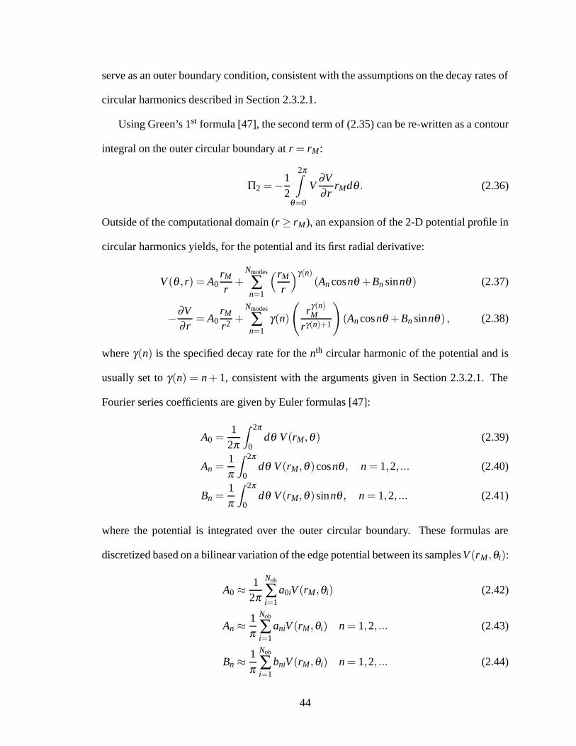
serve as an outer boundary condition, consistent with the assumptions on the decay rates of
circular harmonics described in Section 2.3.2.1.
Using Green’s 1st formula [47], the second term of (2.35) can be re-written as a contour
integral on the outer circular boundary at r = rM:
Π2 =−12
2π∫θ=0
V∂V∂ r
rMdθ . (2.36)
Outside of the computational domain (r ≥ rM), an expansion of the 2-D potential profile in
circular harmonics yields, for the potential and its first radial derivative:
V (θ ,r) = A0rM
r+
Nmodes
∑n=1
(rM
r
)γ(n)(An cosnθ +Bn sinnθ) (2.37)
−∂V∂ r= A0
rM
r2 +Nmodes
∑n=1
γ(n)
(rγ(n)
M
rγ(n)+1
)(An cosnθ +Bn sinnθ) , (2.38)
where γ(n) is the specified decay rate for the nth circular harmonic of the potential and is
usually set to γ(n) = n+ 1, consistent with the arguments given in Section 2.3.2.1. The
Fourier series coefficients are given by Euler formulas [47]:
A0 =1
2π
∫ 2π
0dθ V (rM,θ) (2.39)
An =1π
∫ 2π
0dθ V (rM,θ)cosnθ , n= 1,2, ... (2.40)
Bn =1π
∫ 2π
0dθ V (rM,θ)sinnθ , n= 1,2, ... (2.41)
where the potential is integrated over the outer circular boundary. These formulas are
discretized based on a bilinear variation of the edge potential between its samples V (rM,θi):
A0 ≈1
2π
Nob
∑i=1
a0iV (rM,θi) (2.42)
An ≈1π
Nob
∑i=1
aniV (rM,θi) n= 1,2, ... (2.43)
Bn ≈1π
Nob
∑i=1
bniV (rM,θi) n= 1,2, ... (2.44)
44

where Nob is the number of potential samples on the outer boundary. The coefficients a0i,
ani and bni are obtained by integrating the piecewise-linear representation of the boundary
potential profile along with either 1, cosnθ , or sinnθ over each sub-interval defined by the
outer boundary sample locations, yielding:
a0i =12[mod(θi+1−θi,2π)+mod(θi−θi−1,2π)] (2.45)
ani =(cosnθi− cosnθi−1)
n2mod(θi−θi−1,2π)−(cosnθi+1− cosnθi)
n2mod(θi+1−θi,2π), (2.46)
bni =(sinnθi− sinnθi−1)
n2mod(θi−θi−1,2π)−(sinnθi+1− sinnθi)
n2mod(θi+1−θi,2π)(2.47)
where mod() is the modulo function, and the θi samples are assumed to be ordered in
counter-clockwise (increasing) order. These coefficients are computed for modes n =
0,1,2, ...Nmodes, where Nmodes is chosen sufficiently large to accurately represent the az-
imuthal modes that the outer boundary sampling can support. Typically, Nmodes is chosen
as a few times (10 times, for example) the approximate Nyquist limit, i.e.,
Nmodes = ceil
(10
πmin |mod(θi+1−θi,2π)|
). (2.48)
where the function ceil(·) rounds its argument up to the next integer. In contrast with the
discrete Fourier transform, which gives rise to aliasing when the Nyquist limit is exceeded,
there is no concern for aliasing here, since we have defined the coefficients a0i, ani and
bni based on the continuous Fourier transform of a piecewise-linear boundary potential,
as opposed to having discretized the Fourier integrands, as is done in the discrete Fourier
transform.
We may now put the pieces together to obtain a discrete representation of Π2. Insert-
ing (2.37)–(2.38) into (2.36), we obtain for Π2:
Π2 = π
{A2
0+12
Nmodes
∑n=1
γ(n)(A2
n+B2n
)}. (2.49)
45
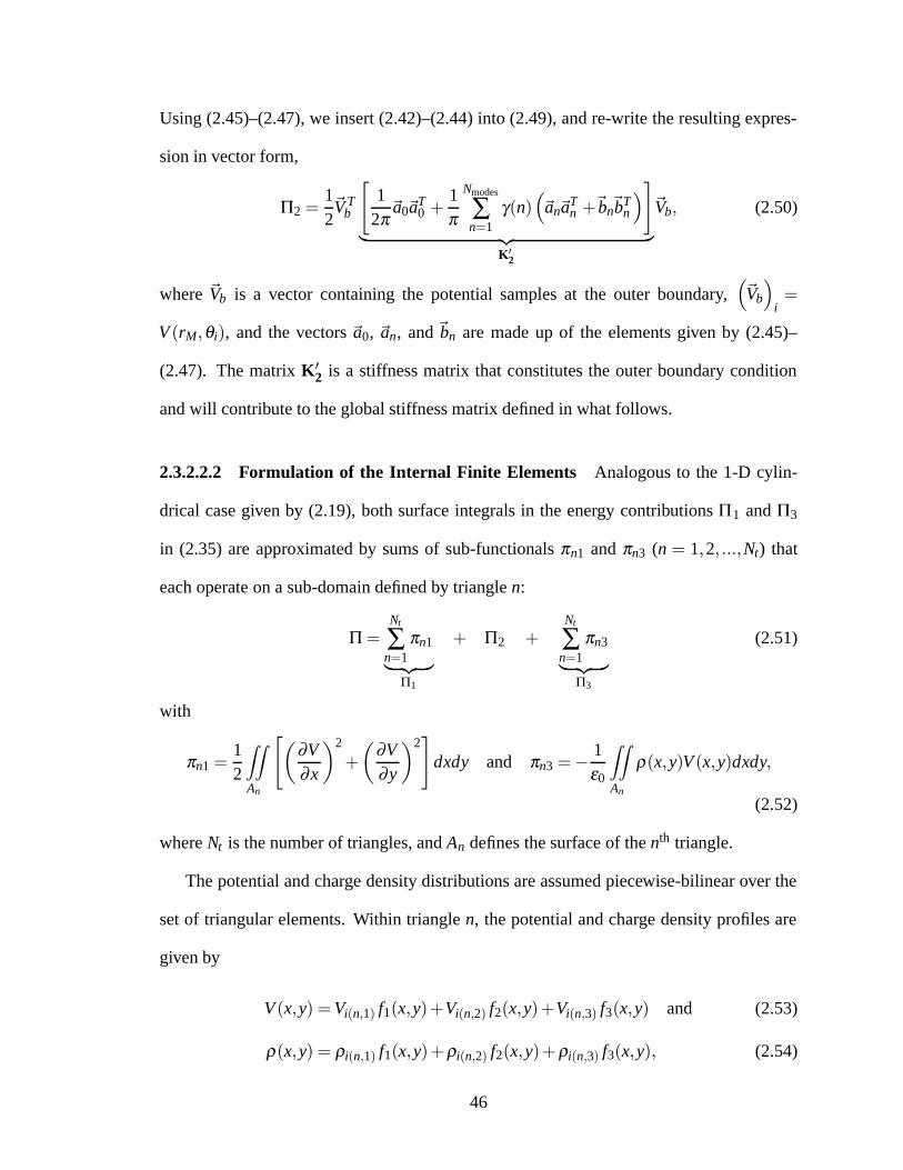
Using (2.45)–(2.47), we insert (2.42)–(2.44) into (2.49), and re-write the resulting expres-
sion in vector form,
Π2 =12�V T
b
[1
2π�a0�a
T0 +
1π
Nmodes
∑n=1
γ(n)(�an�a
Tn +�bn�b
Tn
)]︸ ︷︷ ︸
K′2
�Vb, (2.50)
where �Vb is a vector containing the potential samples at the outer boundary,(�Vb
)i=
V (rM,θi), and the vectors �a0, �an, and �bn are made up of the elements given by (2.45)–
(2.47). The matrix K′2 is a stiffness matrix that constitutes the outer boundary condition
and will contribute to the global stiffness matrix defined in what follows.
2.3.2.2.2 Formulation of the Internal Finite Elements Analogous to the 1-D cylin-
drical case given by (2.19), both surface integrals in the energy contributions Π1 and Π3
in (2.35) are approximated by sums of sub-functionals πn1 and πn3 (n = 1,2, ...,Nt) that
each operate on a sub-domain defined by triangle n:
Π=Nt
∑n=1
πn1︸ ︷︷ ︸Π1
+ Π2 +Nt
∑n=1
πn3︸ ︷︷ ︸Π3
(2.51)
with
πn1 =12
∫∫An
[(∂V∂x
)2
+
(∂V∂y
)2]
dxdy and πn3 =−1ε0
∫∫An
ρ(x,y)V (x,y)dxdy,
(2.52)
where Nt is the number of triangles, and An defines the surface of the nth triangle.
The potential and charge density distributions are assumed piecewise-bilinear over the
set of triangular elements. Within triangle n, the potential and charge density profiles are
given by
V (x,y) =Vi(n,1) f1(x,y)+Vi(n,2) f2(x,y)+Vi(n,3) f3(x,y) and (2.53)
ρ(x,y) = ρi(n,1) f1(x,y)+ρi(n,2) f2(x,y)+ρi(n,3) f3(x,y), (2.54)
46

where the Vi’s and ρi’s are samples of the potential and charge density distributions, and
i(n, :) is a lookup table mapping each of the 3 vertices of triangle n to the corresponding
indices within the vectors of samples �V and �ρ . The fi’s are bilinear interpolation functions
given by
fi(x,y) =(ai+bix+ ciy)
2∆, i= 1,2,3, (2.55)
with coefficients [44]
∆=12|x2y3− x3y2+ x3y1− x1y3+ x1y2− x2y1| ,
a1 = x2y3− x3y2, b1 = y2− y3, c1 = x3− x2,
a2 = x3y1− x1y3, b2 = y3− y1, c2 = x1− x3,
a3 = x1y2− x2y1, b3 = y1− y2, c3 = x2− x1,
(2.56)
where the xi’s and yi’s are the coordinates of the 3 vertices for triangle n and ∆ is the
triangle area. Based on the piecewise-linear description of the potential and charge density
distributions specified by (2.53)–(2.56), approximations for πn1 and πn3 can be written in
matrix form as
πn1 ≈12�V T
i(n,1:3)kn1�Vi(n,1:3) and πn3 ≈−1ε0
�V Ti(n,1:3)Qn�ρi(n,1:3), (2.57)
where kn1, and Qn are both 3×3 matrices. The elements of kn1 are obtained from [44]
(kn1)i j =∫An
(∂ fi
∂x
∂ f j
∂x+
∂ fi
∂y
∂ f j
∂y
)dxdy
=1
4∆(bib j+ cic j
),
(2.58)
where ∆, the bi’s, and the ci’s are defined by (2.56) for triangle n.
Now, finding an expression for the elements of the 3×3 loading matrix Qn is a bit more
involved. The following expression is consistent with πn3 in (2.52), (2.54), and (2.57):
(Qn)i j =1
4∆2
∫An
(a j+b jx+ c jy
)(ai+bix+ ciy) dxdy, (2.59)
47
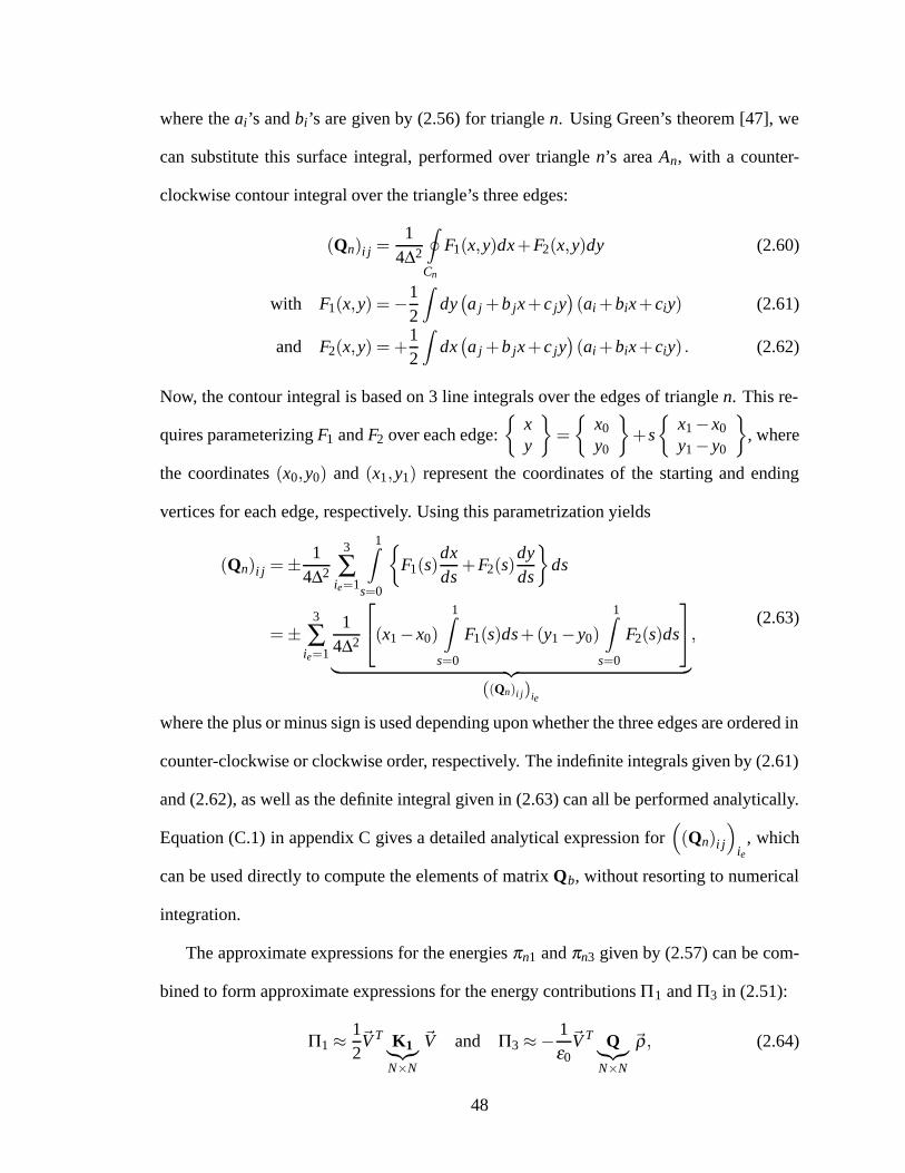
where the ai’s and bi’s are given by (2.56) for triangle n. Using Green’s theorem [47], we
can substitute this surface integral, performed over triangle n’s area An, with a counter-
clockwise contour integral over the triangle’s three edges:
(Qn)i j =1
4∆2
∮Cn
F1(x,y)dx+F2(x,y)dy (2.60)
with F1(x,y) =−12
∫dy(a j+b jx+ c jy
)(ai+bix+ ciy) (2.61)
and F2(x,y) = +12
∫dx(a j+b jx+ c jy
)(ai+bix+ ciy) . (2.62)
Now, the contour integral is based on 3 line integrals over the edges of triangle n. This re-
quires parameterizing F1 and F2 over each edge:
{xy
}=
{x0
y0
}+s
{x1− x0
y1− y0
}, where
the coordinates (x0,y0) and (x1,y1) represent the coordinates of the starting and ending
vertices for each edge, respectively. Using this parametrization yields
(Qn)i j =±1
4∆2
3
∑ie=1
1∫s=0
{F1(s)
dxds+F2(s)
dyds
}ds
=±3
∑ie=1
14∆2
⎡⎣(x1− x0)
1∫s=0
F1(s)ds+(y1− y0)
1∫s=0
F2(s)ds
⎤⎦
︸ ︷︷ ︸((Qn)i j)ie
,(2.63)
where the plus or minus sign is used depending upon whether the three edges are ordered in
counter-clockwise or clockwise order, respectively. The indefinite integrals given by (2.61)
and (2.62), as well as the definite integral given in (2.63) can all be performed analytically.
Equation (C.1) in appendix C gives a detailed analytical expression for((Qn)i j
)ie
, which
can be used directly to compute the elements of matrix Qb, without resorting to numerical
integration.
The approximate expressions for the energies πn1 and πn3 given by (2.57) can be com-
bined to form approximate expressions for the energy contributions Π1 and Π3 in (2.51):
Π1 ≈12�V T K1︸︷︷︸
N×N
�V and Π3 ≈−1ε0
�V T Q︸︷︷︸N×N
�ρ, (2.64)
48
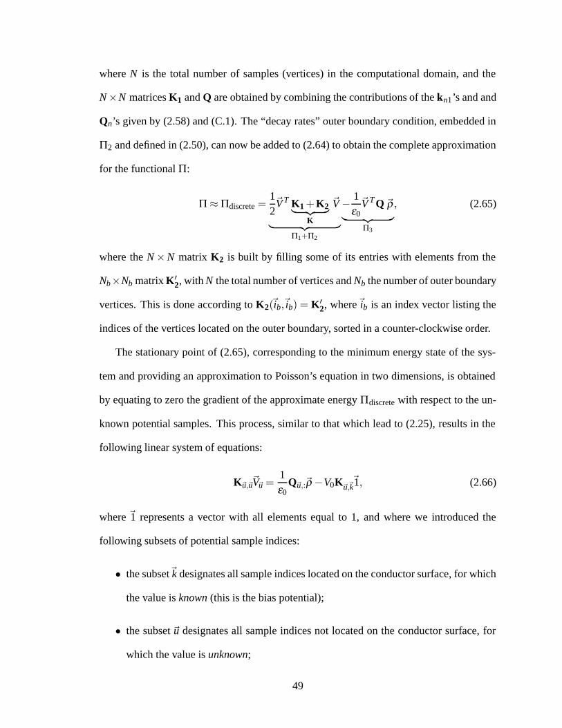
where N is the total number of samples (vertices) in the computational domain, and the
N×N matrices K1 and Q are obtained by combining the contributions of the kn1’s and and
Qn’s given by (2.58) and (C.1). The “decay rates” outer boundary condition, embedded in
Π2 and defined in (2.50), can now be added to (2.64) to obtain the complete approximation
for the functional Π:
Π≈Πdiscrete =12�V T K1+K2︸ ︷︷ ︸
K
�V
︸ ︷︷ ︸Π1+Π2
−1ε0
�V T Q �ρ︸ ︷︷ ︸Π3
, (2.65)
where the N×N matrix K2 is built by filling some of its entries with elements from the
Nb×Nb matrix K′2, with N the total number of vertices and Nb the number of outer boundary
vertices. This is done according to K2(�ib,�ib) = K′2, where�ib is an index vector listing the
indices of the vertices located on the outer boundary, sorted in a counter-clockwise order.
The stationary point of (2.65), corresponding to the minimum energy state of the sys-
tem and providing an approximation to Poisson’s equation in two dimensions, is obtained
by equating to zero the gradient of the approximate energy Πdiscrete with respect to the un-
known potential samples. This process, similar to that which lead to (2.25), results in the
following linear system of equations:
K�u,�u�V�u =1ε0
Q�u,:�ρ−V0K�u,�k�1, (2.66)
where �1 represents a vector with all elements equal to 1, and where we introduced the
following subsets of potential sample indices:
• the subset�k designates all sample indices located on the conductor surface, for which
the value is known (this is the bias potential);
• the subset �u designates all sample indices not located on the conductor surface, for
which the value is unknown;
49

• the use of the colon “:” as a matrix index designates the complete set of potential
samples (same notation as in the Matlab™ scripting language).
We can then solve for the unknown potential samples, analogous to (2.26):
�V�u =
[1ε0
(K�u,�u
)−1 Q�u,:
]︸ ︷︷ ︸
JP′Nu×N
�ρ −V0(K�u,�u
)−1 K�u,�k�1︸ ︷︷ ︸
�V cst′
, (2.67)
where Nu is the number of unknown samples (i.e., the length of �u), and �V cst′ has Nu el-
ements. Finally, we combine this resulting operator with the known potential samples to
form the complete 2-D Poisson solver as follows:
�V = JP�ρ+�V cst, (2.68)
with
JP�u,: = JP′, (2.69)
JP�k,: = [0]Nk×N , (2.70)
�V cst�u =
�V cst′, and (2.71)
�V cst�k=V0�1, (2.72)
where [0]Nk×N is an Nk×N zero matrix. (2.68) gives the final compact form of our finite
element-based 2-D Poisson solver. Just like its 1-D counterpart, it is a linear operator and
only needs to be computed once upon generating a new triangular mesh.
2.4 Steady-State Vlasov Solver
We now derive the Vlasov solver, that is, a numerical approximation for the Vlasov
operator defined above by the functional fV . The Vlasov solver will provide the capability
to find a numerical approximation for the net charge density distribution satisfying Vlasov’s
equation and boundary conditions for the inbound particles.
50
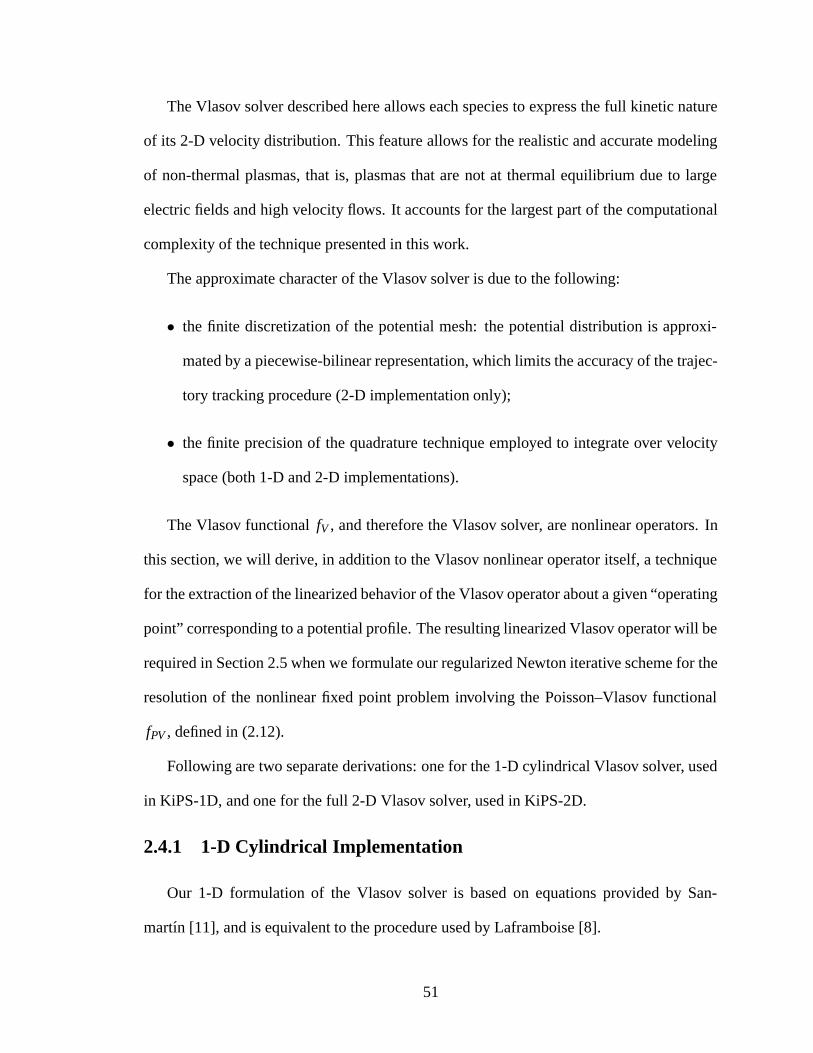
The Vlasov solver described here allows each species to express the full kinetic nature
of its 2-D velocity distribution. This feature allows for the realistic and accurate modeling
of non-thermal plasmas, that is, plasmas that are not at thermal equilibrium due to large
electric fields and high velocity flows. It accounts for the largest part of the computational
complexity of the technique presented in this work.
The approximate character of the Vlasov solver is due to the following:
• the finite discretization of the potential mesh: the potential distribution is approxi-
mated by a piecewise-bilinear representation, which limits the accuracy of the trajec-
tory tracking procedure (2-D implementation only);
• the finite precision of the quadrature technique employed to integrate over velocity
space (both 1-D and 2-D implementations).
The Vlasov functional fV , and therefore the Vlasov solver, are nonlinear operators. In
this section, we will derive, in addition to the Vlasov nonlinear operator itself, a technique
for the extraction of the linearized behavior of the Vlasov operator about a given “operating
point” corresponding to a potential profile. The resulting linearized Vlasov operator will be
required in Section 2.5 when we formulate our regularized Newton iterative scheme for the
resolution of the nonlinear fixed point problem involving the Poisson–Vlasov functional
fPV , defined in (2.12).
Following are two separate derivations: one for the 1-D cylindrical Vlasov solver, used
in KiPS-1D, and one for the full 2-D Vlasov solver, used in KiPS-2D.
2.4.1 1-D Cylindrical Implementation
Our 1-D formulation of the Vlasov solver is based on equations provided by San-
martın [11], and is equivalent to the procedure used by Laframboise [8].
51

2.4.1.1 Approximating the Vlasov Functional fV in 1-D
The potential profile is symmetric about the center of the round cylindrical probe. Since
the only force present is that due to the electrostatic field, we have a central force field.
Because there are no azimuthal forces, the angular momentum L = mrvθ of any particle
is conserved along its trajectory. In addition, the transverse energy of a particle, E =
me,i2
(v2
∞− v2z
), is conserved5:
me,i
2
(v2
r + v2θ)+qV ≡ E, (2.73)
where V is the electric potential, and m and q are the mass and charge of the particle. In
this 1-D formulation, the cylindrical symmetry of the electric field and particle distribu-
tions only allows us to consider the “stationary plasma” case. Both the ion and electron
populations are assumed to have Maxwellian velocity distributions far from the probe, as
r→ ∞:
fe,i (r→ ∞,E,L) =n0 me,i
2π eTe,iexp
(−
EeTe,i
), (2.74)
where we use the invariants E and L as the independent variables for simplicity and to be
consistent with Sanmartın.6 At any given location in space, the velocity distribution is equal
to that given by (2.74) for all energy and angular momentum values (E,L) corresponding
to a trajectory that is connected to infinity, and is assumed unpopulated otherwise. Let us
define L2r (E)≡ 2me,ir2 [E−qe,iV (r)] and recognize that L2
r (E) = L2+m2e,ir
2v2r . We repeat
here, for completeness, the criteria given in [11] for a trajectory to be connected to infinity:
• owing to conservation of energy, only particles with a total energy sufficient to over-
come any electric potential barriers, i.e., particles with an energy
E ≥ Emin =max(0,max
{qV (r′); r ≤ r′ < ∞
}), (2.75)
5v∞ is the particle’s velocity when it is far removed from the probe, i.e., as r −→ ∞.6In this text, the variable L is used for angular momentum, whereas Sanmartın [11] uses the notation J.
52

are connected to infinity;
• an incoming particle can only reach r if its angular momentum L is sufficiently small
to allow v2r to have stayed positive from r′ = ∞ to r′ = r. This specifies an allowed
range that the angular momentum of an incoming particle can have at r:
0< L< L∗r (E) =min{
Lr′(E); r ≤ r′ < ∞}. (2.76)
Particles with a larger angular momentum L> L∗r (E) are thus “reflected” by what is
sometimes described as an effective potential barrier;
• for outgoing particles there is, in addition to an upper bound L∗r (E) on the angular
momentum, a lower bound L∗r0(E) = min{Lr′(E);r0 ≤ r′ < ∞}. Particles having a
lower angular momentum are collected on the probe at r= r0 and thus do not return.
Based on these bounds for the angular momentum, the velocity distribution is given by:
fe,i (r,E,L) =
⎧⎪⎨⎪⎩
fe,i (r→ ∞,E,L) if vr < 0 and 0< L< L∗r (E)
fe,i (r→ ∞,E,L) if vr > 0 and L∗r0(E)< L< L∗r (E)
0 otherwise.
(2.77)
The number density is then obtained by integrating the velocity distribution function over
velocity space, or alternatively, over the 2-D space defined by E and L. The change of
variables (vr,vθ )→ (E,L) implies the following Jacobian:
∂ (vr,vθ )
∂ (E,L)=
∣∣∣∣∣∣∣∣∣∂vr
∂E∂vr
∂L
∂vθ∂E
∂vθ∂L
∣∣∣∣∣∣∣∣∣=
1
m√
L2r (E)−L2
. (2.78)
53

Using this Jacobian and accounting for both positive and negative values of the angular
momentum L, we obtain
ne,i(r) =n0
π eTe,i
∞∫E=Emin
dE exp
(−
EeTe,i
)⎡⎢⎢⎢⎢⎢⎢⎣
L∗r (E)∫L=0
dL√L2
r (E)−L2︸ ︷︷ ︸vr<0
+
L=Lr∗(E)∫L=L∗r0
(E)
dL√L2
r (E)−L2
︸ ︷︷ ︸vr>0
⎤⎥⎥⎥⎥⎥⎥⎦
=n0
π eTe,i
∞∫E=Emin
dE exp
(−
EeTe,i
)⎡⎢⎢⎢⎢⎣sin−1
(L
Lr(E)
)∣∣∣∣L∗r (E)
0︸ ︷︷ ︸vr<0
+sin−1(
LLr(E)
)∣∣∣∣L∗r (E)
L∗r0(E)︸ ︷︷ ︸
vr>0
⎤⎥⎥⎥⎥⎦
=n0
π eTe,i
∞∫E=Emin
dE exp
(−
EeTe,i
)[2sin−1 L∗r (E)
Lr(E)− sin−1 L∗r0
(E)
Lr(E)
],
(2.79)
with Emin as defined in (2.75), and L∗r (E) as defined in (2.76). The integral in (2.79) cannot,
in general, be performed analytically, because of the dependence of L∗r (E) and L∗r0(E) on
part or all of the potential profile through (2.76). This is true even in the case of the orbital
motion limit, a regime in which all trajectories hitting the probe surface at r = r0 are con-
nected to infinity, except for n(r= r0). In the case of OML, L∗r0(E)= Lr0(E) applies, so that
the bracketed expression in (2.79) goes to π/2, resulting in n(r0) = n0/2. However, even
in OML, L∗r (E) < Lr(E) for some positions r, which means that, at several positions, es-
pecially further out from the probe, the integral cannot be performed analytically to obtain
the number density.
In general, it suffices to integrate the exponentially-decaying integrand up to a finite en-
ergy value E = κrangeeTe,i, with a sufficiently large value for κrange, to obtain an acceptable
accuracy on the integral. A value of κrange = 5 is typically chosen, corresponding to an in-
tegrand exp(− E
eTe,i
)∣∣∣E=5eTe,i
= 0.0067, and yielding integration accuracies on the order of
1%. Our 1-D Vlasov solver computes an approximation for this integral to a given relative
54

accuracy εr using a numerical integration technique. We have implemented an adaptive
scheme using the trapezoidal quadrature rule [48] to that effect, which is discussed in Ap-
pendix D. This adaptive quadrature scheme selects a set of abscissa Ek,k = 1,2, ..,Nk,
where the integrand is evaluated, along with associated weights, resulting in the following
approximation for the density profile at locations r = r j, j = 1,2, ...,N:
ne,i(r j)≈ (ne,i) j =n0
π eTe,i
Nk
∑k=1
wk exp
(−
Ek
eTe,i
)[2sin−1
L∗r j(Ek)
Lr j(Ek)− sin−1 L∗r1
(Ek)
Lr j(Ek)
]
with E1 < E2 < ... < Ek < ... < EN−1 < EN,
E1 =max(0,max
{qe,iVj′ ; j ≤ j′ ≤ N
}),
Lr j(Ek) =
{√2me,ir2
j
[Ek−qe,iVj
]Ek ≥ qe,iVj
0 Ek < qe,iVj
, and
L∗r j(Ek) =min
{Lr j′
; j ≤ j′ ≤ N}.
(2.80)
The complete 1-D Vlasov solver computes both density profiles ne(r) and ni(r) by
numerically evaluating (2.80) at a set of radial positions in computational space within the
range r0 < r < rM . It then combines both results to obtain the “output” net charge density
at all sampled locations r j, j = 1,2, ...,N:
ρ(r j)≈ (�ρout) j = qe (ne) j+qi (ni) j , (2.81)
where qe and qi are the electron and ion charge, respectively. The term “output” is used
here to designate the output of the Vlasov solver.
2.4.1.2 Linearizing the 1-D Vlasov Solver
We now proceed to find expressions for the linearized behavior of the discrete Vlasov
operator specified by (2.81) and (2.80), with respect to the samples of the potential profile.
Let us define∂�ρ∂�V
, an N ×N matrix, as the Jacobian of the Vlasov solver, i.e., a matrix
containing the linearized behavior of each net charge density sample as a function of all the
55
potential samples: (∂�ρ∂�V
)jk≡
∂ρ j
∂Vk, j,k = 1,2, ...,N. (2.82)
Based on (2.81) we can define∂�ni
∂�Vand
∂�ne
∂�Vsuch that
∂�ρ∂�V= qe
∂�ne
∂�V+qi
∂�ni
∂�Vas follows:
(∂�ne
∂�V
)j,k≡
∂ (ne) j
∂Vk, j,k= 1,2, ...,N, and (2.83)(
∂�ni
∂�V
)j,k≡
∂ (ni) j
∂Vk, j,k = 1,2, ...,N. (2.84)
Analytical expressions for the elements of these two N×N matrices are fairly compli-
cated and therefore difficult to write in compact form. However, they can be written in a
fairly compact form as an algorithm used to fill the elements, which is done in Algorithm 1,
consistent with (2.80). It should be noted that the Ek’s are samples of the independent vari-
able (the energy), and therefore have no dependence on the potential.
Finally, considering a Vlasov “input” potential profile �Vin, a Vlasov “output” net charge
profile �ρout, and the Jacobian expression JV =∂�ρ∂�V
, the linearized behavior of the Vlasov
solver can be described as
�ρ ∼=�ρout+∂�ρ∂�V
(�V −�Vin
)(2.85)
for any input potential profile �V in the vicinity of �Vin. This linearized behavior will be used
in Section 2.5 for the implementation of the regularized Newton iterative scheme used for
the resolution of the nonlinear fixed point Poisson–Vlasov problem.
2.4.2 Full 2-D Implementation
2.4.2.1 Orbit Tracking and Analysis
The crucial difference between the 1-D Vlasov solver and its 2-D counterpart is that
the latter requires explicit tracking of particle trajectories in order to sample the velocity
distribution function in 2-D velocity space. This requirement is born out of the fact that,
generally speaking, the 2-D potential profile is not rotationally symmetric, i.e., there are
56

Algorithm 1 Algorithm used to compute the elements of the density Jacobian∂�n∂�V
(1-D
cylindrical implementation)
Initialize Jacobian:∂�n∂�V= [0]N×N
for k = 1 to N doif k �= k∗ and L∗rk
(Ek)> 0 then(∂�n∂�V
)k,k=
(∂�n∂�V
)k,k+
qe,in0
π eTe,iwk exp
(−
Ek
eTe,i
)γ
√u
(Ek−qVk)√
1− γ2u,(
∂�n∂�V
)k,k∗=
(∂�n∂�V
)k,k∗−
qe,in0
π eTe,iwk exp
(−
Ek
eTe,i
)γ
1
(Ek−qVk)√
u(1− γ2u),
with γ =r∗krk
and u= 1+qVk−V ∗kEk−qVk
.
end ifif k �= 1∗ and L∗r1
(Ek)> 0 then(∂�n∂�V
)k,1∗=
(∂�n∂�V
)k,1∗+
qe,in0
2π eTe,iwk exp
(−
Ek
eTe,i
)γ ′
√u′
(Ek−qVk)√
1− γ ′2u′,
(∂�n∂�V
)k,1∗=
(∂�n∂�V
)k,1∗−
qe,in0
2π eTe,iwk exp
(−
Ek
eTe,i
)γ ′
1
(Ek−qVk)√
u′(1− γ ′2u′
) ,
with γ ′ =r∗1rk
and u′ = 1+qVk−V ∗1Ek−qVk
.
end ifend forwhere k∗, r∗k and 1∗, r∗1 are such that:L∗rk(Ek)≡ Lr∗k
(Ek)≡ Lrk∗(Ek) =minimum
{Lrk′(Ek) : k ≤ k′ ≤ N
}L∗r1(Ek)≡ Lr∗1
(Ek)≡ Lr1∗(Ek) =minimum
{Lrk′(Ek) : 1≤ k′ ≤ N
}
azimuthal variations of the potential and net charge density distributions. Any particle
trajectory belongs to one of three states:
plasma-bounded trajectories are trajectories originating from the background plasma;
conductor-bounded trajectories are trajectories originating from the surface of a con-
ductor, such as a probe;
trapped trajectories are trajectories of indefinite length, which typically orbit around the
probe.
57

In our basic implementation, only plasma-bounded trajectories are populated. Conductor-
bounded trajectories are left empty, consistent with our assumption of non-emitting con-
ductors; accounting for thermionic emission would require populating those trajectories.
Trapped trajectories are deemed unpopulated because of the absence of collisions to scat-
ter bounded particles into trapped states.7
In the 1-D cylindrical case, conservation of angular momentum L allows for the direct
determination of the state of a particle’s trajectory based solely on its energy E and angular
momentum L, as described in Section 2.4.1. However, since the angular momentum L is not
conserved in the more general 2-D case, an “inside-out” [36] trajectory tracking procedure
is employed in order to determine the origin of each trajectory and therefore its state.
Figure 2.1 illustrates the particle tracking process, which is similar to that used by
Xu [17]. The trajectories are tracked analytically backward in time from one edge of the
mesh to another, assuming a constant electric field within any given triangle of the mesh;
this is consistent with the assumption of a piecewise-bilinear potential distribution. Every
sub-trajectory is resolved by computing the intersection of a quadratic parametric curve
with a segment on the mesh.
Within a given triangle of the mesh, a particle’s trajectory is described by
x= xi+ vixt+12
axt2 and (2.86)
y= yi+ viyt+12
ayt2, (2.87)
where (xi,yi) and (vix,viy) are the initial position and velocity of the particle upon entering
the triangle, t < 0 is the negative time-of-flight8 from the triangle entry, and the constant
7Under certain conditions, however, even very low collision rates can lead to substantial accumulation ofparticles in trapped states [41].
8The time-of-flight is negative since we are tracking trajectories backward in time.
58
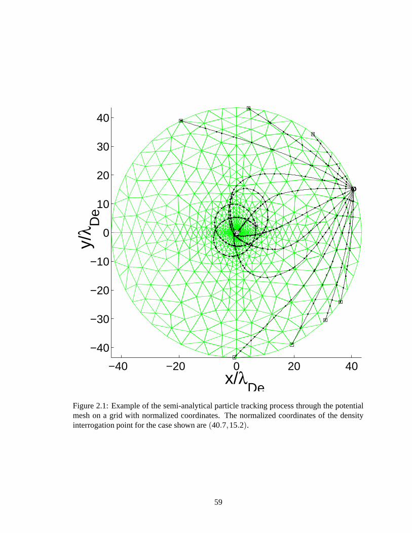
−40 −20 0 20 40
−40
−30
−20
−10
0
10
20
30
40
x/λDe
y/λ D
e
Figure 2.1: Example of the semi-analytical particle tracking process through the potentialmesh on a grid with normalized coordinates. The normalized coordinates of the densityinterrogation point for the case shown are (40.7,15.2).
59

acceleration�a=
{ax
ay
}is obtained from the potential samples at the triangle’s vertices using
�a=qm�E =−
qm
∇V
=−qm[(V1b1+V2b2+V3b3) x+(V1c1+V2c2+V3c3) y]
2∆,
(2.88)
where V1, V2, and V3 are the potential samples at the three vertices of the triangle under
consideration and the bi, ci, and ∆ constants are given by (2.56) as a function of the triangle
vertex coordinates. This trajectory is intersected with each of the three segments, and
the intersection resulting in the shortest time-of-flight is selected as the origin of this sub-
trajectory. Each triangle’s segment can be represented in one of two forms:
z(x,y) = s(y− px−q) = 0 (2.89)
for segments oriented within 45 degrees of the x axis, and
z′(x,y) = s(x− p′y−q′
)= 0 (2.90)
for other segments. In both (2.89) and (2.90), s is chosen as either +1 or −1, such that
z(x,y) or z′(x,y) is made positive inside the triangle and negative outside. Inserting (2.86)
and (2.87) into either (2.89) or (2.90), we obtain
z(t) =s2(ay− pax)︸ ︷︷ ︸
zA
t2+ s(viy− pvix)︸ ︷︷ ︸zB
t+ s(yi− pxi−q)︸ ︷︷ ︸zC
= 0 (2.91)
or
z(t) =s2
(ax− p′ay
)︸ ︷︷ ︸
zA
t2+ s(vix− p′viy
)︸ ︷︷ ︸zB
t+ s(xi− p′yi−q′
)︸ ︷︷ ︸zC
= 0, (2.92)
respectively. Only one of the two roots of z(t), which we define as z(t) = zAt2+ zBt+ zC in
either cases, corresponds to an intersection where the particle is entering the triangle. This
“entering” intersection must satisfy dzdt > 0, since z(t)< 0 outside the triangle and z(t)< 0
inside the triangle. The unique solution that is both a root of z(t) and satisfies dzdt > 0 can
60

Algorithm 2 Numerically stable evaluation of quadratic root
if z2B−4zAzC < 0 then
No real root: trajectory does not intersect segmentelse if zB ≤ 0 and zA ≥ 0 then
No past “entering” root for t < 0else if zB ≤ 0 and zA < 0 then
t←−zB+
√z2
B−4zAzC
2zAelse if zB > 0 then
t←−2zC
zB+√
z2B−4zAzC
end if
be written in two equivalent forms. For numerical stability [48], the roots are evaluated
according to Algorithm 2.
Although both expressions for t in Algorithm 2 are mathematically equivalent, either
one can become numerically unstable, and we must therefore choose the most stable ex-
pression on every evaluation. Our condition ondzdt
is easily verified for both expressions:
dzdt= 2zAt + zB =
√z2
B−4zAzC > 0. The first expression is numerically unstable when
zB > 0, especially when zA is small, due to near cancellation of the two terms in the nu-
merator; a pathological example is that when zA = 0, which leads to t ← −zB+zB0 = 0
0 , an
indeterminate state, while the second expression yields the correct result, t = − zCzB
. The
second expression is numerically unstable when zB ≤ 0, especially when zC is small, due to
near cancellation of the two terms in the denominator; a pathological example is that when
zc = 0, leading to the indeterminate state t← 0zB−zB
= 00 .
This semi-analytical trajectory-tracking technique is much more efficient than using
a fixed time step particle pusher, since the number of computations necessary for each
trajectory depends on the number of edges being crossed rather than the number of time
steps necessary to reach a boundary. This is a highly desirable feature, in light of the fact
that our typical applications (small probes at high voltage) require multi-scale resolution.
61
In addition, given the assumption of a piecewise-bilinear potential distribution, it provides
exact (nearly exact if we account for roundoff errors) conservation of energy along orbits,
which contributes to the accuracy of the overall approach.
2.4.2.1.1 A Note on Segment-bound Trajectories Under certain conditions of the ac-
celerating electric fields in the two triangles surrounding a given mesh segment, some tra-
jectories become bound to that segment, which can give rise to a large number of intersec-
tions with the segment due to tiny oscillations of the trajectory from one side of the segment
to the other. Because this large number of intersections can significantly slow down com-
putations, this case is treated as an exception. When such infinitesimal oscillations are
detected, the oscillating portion of the trajectory is resolved using only the tangential ve-
locity and acceleration along the segment. This process does not reduce the accuracy of the
trajectory tracking in any way.
2.4.2.2 Sampling the Velocity Distribution Function
In collisionless plasmas, the velocity distribution function f (x,y,vx,vy) is conserved
along particle orbits [25], which allows one to infer the value of f (x f ,y f ,vx f ,vy f ) at a
final position (x f ,y f ) and velocity (vx f ,vy f ), based on its initial value f (xi,yi,vxi,vyi) at the
origin of the particle’s trajectory, at a position (xi,yi) and velocity (vxi,vyi).
Using the semi-analytical trajectory-tracking procedure just described, we may deter-
mine the origin of a given particle trajectory, and thus sample the velocity distribution
function. This is typically referred to as the inside-out technique [36] in plasma modeling
and, more generally, as the method of characteristics [49] for solving partial differential
equations (here, the collisionless Vlasov equation).
For plasma-bounded trajectories, the reverse-time tracking procedure eventually gets
to the outer boundary of the computational domain (its origin), at a position (xi,yi) with
62

an “initial” velocity (vxi,vyi). The velocity distribution at the “final” position (x f ,y f ) and
velocity (vx f ,vy f ) can therefore be sampled based on the known velocity distribution on the
outer boundary. The fact that the potential is floating on the outer boundary implies that the
velocity distribution function at that location, f i(vxi,vyi) = f (xi,yi,vxi,vyi), is different than
the velocity distribution function f∞(vx∞,vy∞) at infinity. Since the electric fields are not
modeled from r=∞ to the outer boundary of the computational domain, an approximation
must be made to infer fi from f∞.
For this purpose, we use the “straight-line approximation”. This approximation con-
sists of assuming straight-line trajectories from infinity to the outer boundary of the com-
putational domain. Particles in the drifting Maxwellian population at r = ∞ are assumed
to be accelerated along straight lines in the direction pointed to by their initial velocity, all
the way to the point where they intersect the outer boundary of the computational domain.
Based on this assumption, a drifting Maxwellian at infinity, given by
f∞ (vx∞,vy∞) =n0me,i
2πeTe,iexp
{−
me,i
2eTe,i
((vx∞−U)2+ v2
y∞
)}, (2.93)
where U is the flow speed of the background plasma, would be mapped to the following
distribution on the outer boundary of the computational domain:
fi (xi,yi,vxi,vyi) =n0me,i
2πeTe,iexp
{−
me,i
2eTe,i
(2
qe,i
me,iVedge+ v2
xi+ v2yi+U2
−2Uvxi
√√√√v2xi+ v2
yi+2 qe,ime,i
Vedge
v2xi+ v2
yi
⎞⎟⎠⎫⎪⎬⎪⎭ , (2.94)
where Vedge is the potential at the entry point on the outer boundary of the computational
domain. This method was used for the calculations performed by Godard and Lafram-
boise [30]. Its main advantage is that it provides a smooth transition to the stationary case
where U = 0, in which case we simply recover the exact accelerated Maxwellian distribu-
tion. The expression given by (2.94) is no longer an approximation when U = 0 because,
63

in this case, the velocity distribution function samples do not depends on trajectories, they
simply depend on total energy, just like in the 1-D model.
The reverse-time tracking procedure eventually traces the origin of conductor-bounded
trajectories back to the surface of the probe or other conducting surfaces. Since the con-
ductors are not emitting particles, we assume that these trajectories are unpopulated and set
fe,i(x f ,y f ,vx f ,vy f
)= 0.
Trapped trajectories, defined earlier in this section, are deemed unpopulated just like
conductor-bounded trajectories. Thus, the velocity distribution function sample for tra-
jectories identified as trapped is set to zero. The main difficulty with these trajectories,
however, resides in the determination of the trapped state. Since, by definition, trapped tra-
jectories orbit indefinitely, a set of criteria must be used to determine whether a trajectory
being followed is actually trapped:
Maximum angular displacement The angular displacement of the particle is integrated
over time, i.e.,
θvar =
t f∫t=ti
∣∣∣∣dθ(t)dt
∣∣∣∣dt. (2.95)
When this quantity goes beyond 2πMorb, the trajectory is deemed trapped. Typically,
Morb is set to 3, which, for a trajectory orbiting in a constant orientation along θ ,
corresponds to 3 full orbits about the origin.
Maximum number of radial oscillations Beyond a given number Mrosc of significant os-
cillations of the particle’s radial coordinate r, the trajectory is assumed trapped. Typ-
ically, Mrosc is set to 5. This parameter is discussed in more detail in Section 4.3.2.1.
Maximum number of intersections of any single edge When the trajectory intersects a
given edge, within the mesh, more than a given number Msegcross of times, the trajec-
tory is assumed trapped. Typically, Msegcross is set to 100.
64
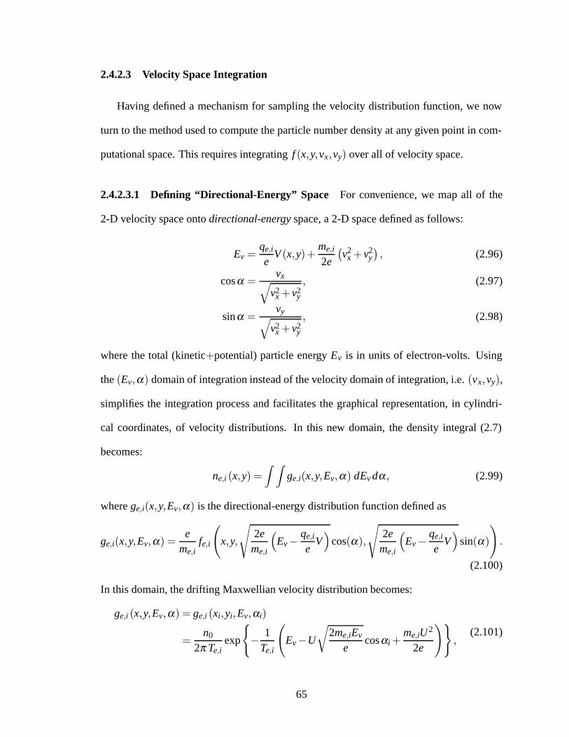
2.4.2.3 Velocity Space Integration
Having defined a mechanism for sampling the velocity distribution function, we now
turn to the method used to compute the particle number density at any given point in com-
putational space. This requires integrating f (x,y,vx,vy) over all of velocity space.
2.4.2.3.1 Defining “Directional-Energy” Space For convenience, we map all of the
2-D velocity space onto directional-energy space, a 2-D space defined as follows:
Ev =qe,i
eV (x,y)+
me,i
2e
(v2
x+ v2y
), (2.96)
cosα =vx√
v2x+ v2
y
, (2.97)
sinα =vy√
v2x+ v2
y
, (2.98)
where the total (kinetic+potential) particle energy Ev is in units of electron-volts. Using
the (Ev,α) domain of integration instead of the velocity domain of integration, i.e. (vx,vy),
simplifies the integration process and facilitates the graphical representation, in cylindri-
cal coordinates, of velocity distributions. In this new domain, the density integral (2.7)
becomes:
ne,i (x,y) =∫ ∫
ge,i(x,y,Ev,α) dEv dα, (2.99)
where ge,i(x,y,Ev,α) is the directional-energy distribution function defined as
ge,i(x,y,Ev,α) =e
me,ife,i
(x,y,
√2e
me,i
(Ev−
qe,i
eV)
cos(α),
√2e
me,i
(Ev−
qe,i
eV)
sin(α)
).
(2.100)
In this domain, the drifting Maxwellian velocity distribution becomes:
ge,i (x,y,Ev,α) = ge,i (xi,yi,Ev,αi)
=n0
2π Te,iexp
{−
1Te,i
(Ev−U
√2me,iEv
ecosαi+
me,iU2
2e
)},
(2.101)
65

where the index i refers to the entry (or “initial”) point of the particle at the outer boundary
of computational space, and the total energy Ev is conserved all along the trajectory from
(xi,yi) to (x,y).
To limit the computational task, we restrict the domain of integration to a finite annular
region within directional-energy space, outside of which ge,i(x,y,Ev,α) is known to be very
low:
Ev,min =max
(qe,i
eV (x,y),
(√me,i
2eU−
√κrangeTe,i
)2)
(2.102)
Ev,max =
(√me,i
2eU+
√κrangeTe,i
)2
. (2.103)
Outside of those bounds for the energy Ev, the exponential factor in (2.101) is guaran-
teed to be lower than exp{−κrange}. We typically choose κrange = 5, corresponding to
exp{−κrange}∣∣κrange=5 = 0.0067. This means that we are neglecting the integrand wherever
its value goes below 0.67% of its maximum value (see discussion on page 54).
2.4.2.3.2 Numerical Integration in “Directional-Energy” Space Based on the new
directional-energy space defined above, we numerically integrate ge,i(x,y,Ev,α) within the
rectangular domain given by:
Ev,min ≤Ev ≤ Ev,max (2.104)
0≤α ≤ 2π. (2.105)
Several numerical quadrature schemes were considered, such as an adaptive cubature of
triangular elements [50,51]. As it turns out, however, this technique, as well as other high-
order automatic quadrature routines available, are most suitable for smooth integrands.
Even though (2.101) does appear to be a smooth function, the directional-energy do-
main defined above is only partly covered with plasma-bounded trajectories. Some sub-
66

domains are populated with conductor-bounded and trapped trajectories, for which the dis-
tribution function ge,i(x,y,Ev,α) is set to zero. This creates major discontinuities in the
integrand, which are best represented and integrated using simple first-order polynomials.
Consistent with those findings, a low-order numerical scheme was implemented using
a 2-D iterated integral, based on a single-variable adaptive trapezoidal quadrature [48]. The
outer integral is performed along the direction α:
n(x,y) =
2π∫α=0
I1(x,y,α)dα ≈Nα
∑kα=1
wkα I1(x,y,αkα )≡ nest(x,y), (2.106)
with the integrand I1(x,y,αkα ) obtained by integrating along the energy Ev (inner inte-
grand),
Ev,max∫Ev=Ev,min
ge,i (x,y,Ev,αkα )dEv ≈NE(kα)
∑kE=1
wkα ,kE ge,i(x,y,Ekα ,kE ,αkα
)= I1(x,y,αkα ), (2.107)
where we have explicitly indicated the dependence of the inner quadrature coefficients
wkα ,kE , the energy samples Ekα ,kE = Ev (kα ,kE) and the number of energy samples NE(kα)
on the azimuthal sample number kα .
For each one-dimensional quadrature, the domain of integration is sub-divided into a set
number of sub-intervals, typically 25 along Ev and 45 along α . The integral over each sub-
interval is then initially performed using both 2-point and 3-point trapezoidal rules [48].
The difference between the 2-point and 3-point quadratures is used as an estimate of the
quadrature error. The sub-integrals are then refined by increasing the number of points
used with the trapezoidal rule, providing improved sub-integrals and error estimates. This
refinement is performed on the sub-integrals in decreasing order of quadrature error, until
the total estimated error δnest over the collection of sub-intervals is small enough that
δnest ≤ τrelnest, where δnest is the estimated error on nest, and τrel is a relative tolerance
on the integration error.
67

Let us consider the outer quadrature given by (2.106). In addition to the error caused by
this quadrature approximation, there is a second error term caused by the error δ I1(x,y,αkα )
on the integrand I1(x,y,αkα ), which stems from the error generated by the inner quadrature
given by (2.107). However, if we assume that the errors δ I1(x,y,αkα ), kα = 1, ...,Nα are not
correlated and use the same relative error τrel for the inner quadrature as we do for the outer
quadrature, then the total error term contributed by those integrand errors can be considered
small as compared to the quadrature error δnest = τrelnest on the outer quadrature:
Nα
∑kα=1
wkα δ I1(x,y,αkα ) =Nα
∑kα=1
wkα pkα τrelI1(x,y,αkα )<< τrelnest, (2.108)
where pkα = ±1 is a random phase factor. This justifies using the same relative tolerance
for both the inner and outer quadratures.
In addition to the use of a relative error tolerance, an absolute error tolerance is also
used, in order to prevent excessive refinements of the inner quadrature. For some values of
kα , the integrand I1(x,y,αkα ) can take on relatively small values, contributing very little to
nest, and therefore need not be computed with an accuracy as good as that specified by the
relative tolerance. Let us assume that we can tolerate an additional error term to nest, on the
same order of magnitude as δnest = τrelnest, which, if we spread it out over the integrand
I1(x,y,α), determines an absolute tolerance on the values computed for I1(x,y,αkα ):
τabs,E =τrelnest
2π. (2.109)
Since the value for τabs,E is required in advance, i.e., before having computed a value for
nest, we use our best available estimate for nest to compute τabs,E , that is, the value obtained
at the previous iteration of the iterative process (see Section 2.5). Finally, for the same
reasons mentioned earlier, the non-correlated addition of the error terms caused by the
use of this absolute error tolerance actually contributes much less than the outer-integral
quadrature error δnest = τrelnest. Therefore, for all practical purposes, we need not account
68
for this error term within δnest.
We hereby summarize the complete quadrature process:
• The inner quadrature dynamically selects, using adaptive trapezoidal rules on a set
of sub-intervals, the energy samples Ekα ,kE , kE = 1, ...,NE(kα) and corresponding
weights wkα ,kE that are required in order to compute I1(x,y,αkα ) with a relative accu-
racy τrel such that
δ I1(x,y,αkα )≤ τrelI1(x,y,αkα )+ τrelnest,prev
2π(2.110)
with nest,prev an estimate for the density based on the previous iteration.
• The outer quadrature dynamically selects, using adaptive trapezoidal rules on a set of
sub-intervals, the direction samples αkα , kα = 1, ...,Nα and corresponding weights
wkα that are required in order to compute the estimate nest(x,y) for the density n(x,y)
with an accuracy
δnest ≤ τrelnest. (2.111)
• The net result of those two embedded quadratures is an approximate number density
n j ≡ n(x j,y j) =Nα
∑kα=1
wkα
NE(kα )
∑kE=1
wkα ,kE ge,i(x,y,Ekα ,kE ,αkα ), (2.112)
where wkα and αkα are selected by the α-quadrature, while wkα ,kE and Ekα ,kE are
selected by the E-quadrature. Finally, both the electron and ion number density
estimates at all node locations are combined into the net charge density �ρ through
the expression
ρ(x j,y j) = (�ρout) j = qe (ne) j+qi (ni) j . (2.113)
69

2.4.2.4 Linearizing the 2-D Vlasov Solver
The linearization of the 2-D Vlasov operator is similar to that of the 1-D Vlasov opera-
tor. It provides a Jacobian matrix JV =∂�fV
∂�V=
∂�ρout
∂�Vthat describes the linear dependence
of the output charge distribution onto the potential distribution.
Appendix E details the linearization process used for the 2-D Vlasov solver. It describes
two different techniques that are used alternatively for stationary and flowing problems,
respectively, along with sources of error in the calculation of the Jacobian.
2.5 Regularized Newton Iterative Poisson–Vlasov Scheme
Using the Poisson and Vlasov solvers, we now seek to find a solution for the poten-
tial and charge distributions that satisfies both the Poisson and Vlasov equations. We have
seen that this task is equivalent to finding the fixed point of the Poisson–Vlasov functional
defined in (2.12) and illustrated in Figure 2.2. In Sections 2.3 and 2.4, we have defined
Poisson and Vlasov solvers that are numerical approximations of the Poisson (2.10) and
Vlasov (2.11) operators, respectively. In Table 2.2, we show the correspondence between
the functional and associated numerical solver for the Poisson, Vlasov, and Poisson–Vlasov
operators. As can be seen in that table, we distinguish the functionals from their corre-
sponding numerical solvers by putting an arrow on top of the symbols used for the opera-
tors, which were defined in Section 2.2. The newly defined functions �fP, �fV and �fPV are
thus all multi-valued functions of multiple variables.
There are known difficulties arising in finding the fixed point of a multivalued, multi-
variate function [8]. Simple iteration of the fixed point operator does not in general yield
convergence, since it is a non-contractive mapping [52]. Laframboise [8], Xu [17], and
McMahon [22] use a method consisting of mixing consecutive iterates using empirically-
determined mixing functions. Because of the breadth of regimes sought as part of this
70

Operator Functional Numerical Solver
Poisson V (x,y) = fP {ρ(x,y} �V = �fP {�ρin}
Vlasov ρ(x,y) = fV {V (x,y)} �ρout = �fV{�V}
Poisson–Vlasov ρout(x,y) = fPV {ρin(x,y)} �ρout = �fPV {�ρin}
Table 2.2: Functional operators and corresponding numerical solvers. The Poisson–Vlasovfunctional is defined as a composition of the Poisson and Vlasov functionals, so that�fPV {·}= �fV
{�fP {·}
}.
research (low and high voltages, arbitrary geometries, plasma flow), we found that the it-
erate mixing method could not provide a repeatable and reliable automated technique for
finding accurate approximations to the fixed point of the Poisson–Vlasov operator in a rea-
sonable number of iterations. This is especially true when modeling two kinetic species
and in regimes comprising high voltages and various probe geometries.
2.5.1 Top-level Iterative Scheme
To address these difficulties, we have chosen to implement a procedure based on New-
ton’s method for nonlinear systems of equations [53]. This technique, which we desig-
nate as the Progressive Tikhonov-regularized Newton iterative Poisson–Vlasov procedure,
is depicted in Figure 2.3. It consists of progressively improving a solution vector �ρin, i.e.,
reducing the residual norm ‖�ρin−�ρout‖, by successively linearizing the Poisson–Vlasov
PoissonSolver
VlasovSolver
�ρin
�V
�ρout
Poisson-Vlasov Operator �fPV
Figure 2.2: Poisson–Vlasov operator comprised of both the Poisson and Vlasov solvers.This operator is an approximation of the Poisson–Vlasov functional defined in (2.12).
71

PoissonSolver
VlasovSolver
�ρin �V �ρout
Poisson-Vlasov Operator �fPV
Tikhonov-Regularized Inversion
�ρ ≈ �ρout + JPV (�ρ − �ρin)
�ρin + β (JPV − I)† (�ρin − �ρout)
Step Size Control
Figure 2.3: Tikhonov-regularized Newton iterative Poisson–Vlasov procedure.
operator and finding a regularized solution for the resulting linearized system of equations.
This process relaxes the solution vector �ρin and has the global effect of reducing the Eu-
clidean distance between�ρin and�ρout. The iterative process continues until the solution can
no longer be improved with the specified quadrature accuracy used in the Vlasov solver.
In practice, a suitable quadrature accuracy is chosen that allows the iterates to reach a rea-
sonably low residual norm ‖�ρin−�ρout‖∞, on the order of one percent of the background
plasma density.
This iterative procedure requires the N×N Jacobian matrix JPV of the Poisson–Vlasov
operator, which is defined as
JPV =∂�fPV
∂�ρ
∣∣∣∣∣�ρ=�ρin
(2.114)
and can be obtained, using the chain rule, as a combination of the Jacobian matrices of the
72

Poisson and Vlasov operators, following
JPV =∂�fV
∂�V×
∂�fP
∂�ρ
∣∣∣∣∣�ρ=�ρin
=∂�ρout
∂�V︸ ︷︷ ︸JV
∂�V∂�ρin︸︷︷︸
JP
= JV JP, (2.115)
where the Jacobian of the Poisson operator was simply recognized as the matrix in the
linear Poisson operator, as obtained for KiPS-1D in (2.27) and for KiPS-2D in (2.68). The
Jacobian of the Vlasov solver, JV , was derived in Sections 2.4.1.2 and 2.4.2.4, where we
discussed the linearization of the Vlasov operator in the 1-D and 2-D solvers, respectively.
In its simplest form, the Newton method [53] attempts to use the linearized behavior
of a multivalued function of several variables to solve a nonlinear system of equations. In
the present case, we are looking for the fixed point of the Poisson–Vlasov operator or, put
differently, we are looking for the vectorial root of the vectorial equation
�g(�ρ) = �fPV (�ρ)−�ρ = 0, (2.116)
which, upon approximating �fPV by its first-order Taylor expansion
�fPV (�ρ)≈�ρout+JPV (�ρ−�ρin) , (2.117)
yields a linear system of N equations in N variables,
[JPV − I] (�ρ−�ρin) =�ρin−�ρout, (2.118)
where the unknown vector �ρ−�ρin is an incremental improvement that will be added to the
present guess �ρin of the charge density distribution, and I is the N×N identity matrix.
2.5.2 Conditioning and Quadrature Noise Issues
One is first tempted to simply invert the system matrix and compute the corrected charge
density distribution according to
�ρin←�ρin+[JPV − I]−1 (�ρin−�ρout) , (2.119)
73

which can be performed using standard linear algebra algorithms such as the LU decompo-
sition [54]. Such an attempt, however, is in general met with wild, non-physical variations
in the charge density distribution �ρin at some point during the iterative process, and al-
most never leads to a convergence of the result to a low ‖�ρin−�ρout‖∞ error state. This
diverging behavior is generally due to the ill-conditioning of the system matrix [JPV − I]
for some iterates, which can greatly amplify any quadrature noise present in the error vec-
tor (�ρin−�ρout). The ill-conditioning of the system matrix can be due to a combination of
several causes, some of which we identify here.
Ill-conditioning of the Vlasov operator, which can be due to the weak or inexistent de-
pendence of most particle trajectories upon some samples of the potential, at various
“operating points” of the potential solution vector �V (near or far from the physical
solution).
Ill-conditioning of the Poisson operator due to a high mesh density in some locations
that creates very similar dependences to some of the densely packed charge samples,
thereby causing highly similar lines in the Poisson matrix JP, defined in Section 2.3.
Incomplete entries in the Vlasov Jacobian JV due to the fact that some components of
the linearized dependence upon the potential samples �V could not be fully accounted
for by the approximate gradient calculation (this only applies to the 2-D version —
see Section 2.4.2.4).
Because of the ill-posedness of this problem, the standard Newton method turns out to
be impractical for the resolution of this nonlinear system of equations. In the following, we
will describe a diagonal scaling technique and a nonlinear regularization method to address
this conditioning issue.
74

Even though our nonlinear system (2.116) does not contain any noisy data per se, the
right-hand side of the linearized system (2.118) is noisy due to the finite precision used in
calculating the output charge profile �ρout = �fPV (�ρin), which we emphasize here:
[JPV − I] (�ρ−�ρin) =�ρin− �ρout︸︷︷︸�ρout+δ�ρout
, (2.120)
where δ�ρout is the quadrature noise term. Recall that the output charge profile �ρout is
computed based on subtracting the electron and ion charge profiles,
�ρout = e(�ni−�ne) , (2.121)
which implies that any numerical quadrature error in the calculation of the density profiles
�ni and�ne can lead to a large relative error ‖δ�ρout‖‖�ρout‖
wherever the electron and ion densities are
very similar, leading to a subtraction of like terms. This situation arises close to the outer
boundary of the computational domain, which is typically sized large enough to enclose all
of the significant charge imbalance, that is, all of the sheath and some of the pre-sheath.
2.5.3 Diagonal Preconditioning
One of the simplest measures that can be taken in order to mitigate the propagation of
the quadrature errors present on the RHS of (2.120) to the incremental solution�ρ−�ρin is to
perform a diagonal preconditioning of the linear system, in an effort to reduce the condition
number of the system matrix. Let us first re-cast the linearized system of interest (2.120)
into the following standard form:
A�x=�b=�b+δ�b, (2.122)
where A ≡ [JPV − I], �b ≡ �ρin−�ρout, �x ≡ (�ρ−�ρin) and the quadrature noise is given by
δ�b≡ −δ�ρout. The vector�x thus constitutes an increment to the present state of the charge
profile�ρin. We choose to use a diagonal right preconditioner [54] Dp that must approximate
75

A−1 as best as possible without actually inverting A, in such a manner as to make the
product ADp closer to the identity matrix. Inserting DpD−1p into (2.122), we write:
ADp︸︷︷︸A′
(D−1
p �x)︸ ︷︷ ︸
�x ′
=�b. (2.123)
To solve (2.122), we will therefore first solve A′�x ′ =�b, and then compute�x using�x=Dp�x ′.
For the class of problems at hand, it was found that setting the entries of the diagonal
matrix Dp equal to the inverse of the norm of the corresponding column vectors of A
yielded the best results:
Dp :
{i= j (Dp)i j =
1‖A:,i‖2
i �= j (Dp)i j = 0,(2.124)
where ‖A:,i‖2 is the Euclidean norm of the ith column of the system matrix A. Using this
preconditioner, the scaled solution vector �x ′ has its elements scaled proportional to the
level of dependence of the system matrix A on each element of �x, thereby improving the
signal-to-noise ratio on the elements of�x upon which the system is most dependent.
Even though preconditioning is essential and improves the condition of the linearized
system, it is simply not sufficient to fully prevent quadrature noise from entering the solu-
tion vector. The regularization process described below will complete the required set of
tools for an accurate resolution of the nonlinear systems at hand.
2.5.4 Tikhonov “Progressive” Regularization
In this section we will describe the complete regularization procedure, which we repre-
sent as a “Tikhonov-regularized inversion” in Figure 2.3.
The topic of regularization of linear systems of equations has attained a very good
maturity level [55–60] and is extensively used for inverse linear problems involving noisy
data in applications such as ionospheric characterizations [61]. A typical linear inverse
problem involving noisy data is of the form A�x=�y=�y0+�δ , where�y contains some noisy
76

data and�x is a set of unknown parameters.
Nonlinear inversion has also seen significant progress [62–66]. It consists of looking
for a solution�x to a nonlinear system of equations of the form
�F(�x) =�y=�y0+�δ , (2.125)
where �F is a nonlinear multivalued function of several variables,�y contains noisy data, and
�x is the set of unknown parameters.
Our problem of interest is different from nonlinear inversion in that we are not trying
to “invert” a nonlinear function given a specified noisy data set. Instead, we are looking for
the fixed point of a nonlinear function �fPV (�ρ), i.e., the root of the nonlinear function �g(�ρ)
as specified by (2.116). This is equivalent to solving a nonlinear system of the form given
by (2.125) with�y= 0.
We therefore seek a method to limit the amount of quadrature noise entering the so-
lution vector �ρin at every iteration, while still allowing a significant improvement of the
solution. Instead of directly solving the preconditioned linear system of equations (2.123),
we seek a compromise between the reduction of the error ‖A′�x ′ −�b‖ and the amount of
noise “creeping into” the solution. A useful compromise is one that would prevent any
significant magnification of the noise present in �b by the inversion of the ill-conditioned
system matrix A′, while still significantly reducing the error ‖A′�x ′ −�b‖. This can be ac-
complished by solving only for the “modes” in �x ′ upon which the preconditioned system
matrix A′ is most dependent, effectively filtering out the more independent, higher-order
“modes” that are very sensitive to any noise in�b.
The “modes” we refer to here correspond to the set of singular values of the precondi-
tioned system matrix A′. Using the singular value decomposition [54], the N×N matrix
77

A′ can be factorized to the form:
A′ =U diag(�σ) VT , (2.126)
where diag(�σ) is a diagonal matrix whose diagonal is formed by the N elements of the
vector�σ , which are the singular values of A′ numbered in descending order, σ1≥σ2≥ ...≥
σn ≥ 0. U and V are both N×N unitary matrices. Recasting the system equation (2.123)
based on this transformation yields:
diag(�σ) VT�x ′ = UT�b (2.127)
or
diag(�σ)x= b, (2.128)
with
x=VT�x ′ and b=UT�b. (2.129)
The linearized system has been re-written in a vector space corresponding to the singular
values of the system matrix A, yielding a set of uncoupled linear relationships between the
corresponding components of x and b:
σ1x1 = b1
σ2x2 = b2
...
σNxN = bN.
(2.130)
In this transformed vector space, a direct inversion of the linearized system is performed
by simply solving each mode separately using
xi =bi
σi. (2.131)
Now, an ill-conditioned matrix A has some extremely small singular values σ i for large i,
potentially resulting in extremely large amplitudes for some of the xi’s, along with signifi-
cant amplification of the noise present in the corresponding bi’s.
78
Setting an appropriate “low-pass” filter to allow the lowest-order modes corresponding
to the largest singular values of σi while blocking the high-order modes corresponding to
the smallest singular values of σi would accomplish our goal of somewhat improving upon
the current guess �ρin while limiting the amount of noise creeping into the solution. The
Tikhonov regularization [56, 58] implements such a continuous “low-pass” filter. Instead
of directly solving for x using (2.131), the Tikhonov-regularized inversion is implemented
as
xi =σi
σ 2i +λ 2
bi, (2.132)
effectively shutting down the high-order modes corresponding to small singular values for
which σi < λ . A mathematically equivalent form of the Tikhonov regularization exists in
the non-transformed domain, as a replacement for the simple inversion�x ′ = [A′]−1�b:
�x ′ =[A′T A′+λ 2I
]−1A′T�b. (2.133)
For our application, the Tikhonov-regularization parameter λ is tuned according to the
following criteria: the targeted error is to be equal to half of the present error, in order to
achieve some progress while limiting the amount of noise creeping into the solution. This
prudent requirement constitutes the basis of the proposed progressive Tikhonov regulariza-
tion. It has been shown in practice to prevent divergence due to the ill-conditioning of the
system matrix, while allowing for significant reduction of the present error ‖�ρin−�ρout‖2.
This criteria can be written as
‖�b−A′�x ′λ‖2 = 0.5‖�b‖2 (2.134)
or, using the original notation,
‖(�ρin−�ρout)− [JPV − I]�xλ‖2 = 0.5‖�ρin−�ρout‖2 . (2.135)
In these two expressions,�x ′λ and�xλ both correspond to the result from (2.133) for a given
79

value of the regularization parameter λ , and are related through �xλ = Dp�x ′λ . At each it-
eration, an optimal value for λ must be determined that satisfies the equivalent expres-
sions (2.134) and (2.135). This is done in one of two ways:
• If the dimension of the system matrix, N, is not too large (say N < 1000), A′ is
first factored into a set of singular values and corresponding unitary matrices U and
V, consistent with (2.126), using the singular value decomposition algorithm [54].
(2.134) is then solved by numerically solving for λ the equivalent expression
N
∑i=1
λ 4(σ 2
i +λ 2)2 b2
i =14
N
∑i=1
b2i , (2.136)
using an appropriate numerical root-finding algorithm (we use the function fminnbd()
provided as part of the Matlab™ software package).
• If the dimension of the system matrix N is too large (N > 1000) for the singular
value decomposition to be performed quickly, then equations (2.134) and (2.133)
are used to numerically solve for λ with reasonable accuracy. This method is more
computationally economical than the previous one since, by using the optimal value
of λ obtained at the previous iteration, as few as 10 trials are typically necessary
to re-optimize for λ . For large N, 10 linear system resolutions of an N×N system
as performed in (2.133) are done much faster than one singular value decomposi-
tion (e.g., for N = 1000, it takes about 65 times longer to perform a singular value
decomposition than to perform an LU decomposition.9)
This progressive regularization strategy enables the iterative refinement procedure to safely
get through the highly singular iterates, that is, the iterates for which the system ma-
trix A= [JPV − I] is quasi-singular, without diverging. The net effect of the progressive
9Based on a benchmark performed on a Linux-based Matlab ™ 6.0 engine.
80

Tikhonov regularization is that the incremental correction of the solution vector dominates
over the addition of quadrature noise, resulting in a net improvement of the solution.
The combination of the diagonal preconditioner, described in Section 2.5.3 and the reg-
ularized inversion described in this section constitute the “Tikhonov-regularized inversion”
and are represented using the symbol † in Figure 2.3. The complete Tikhonov-regularized
inversion referred to in Figure 2.3 can thus be written as
∆�ρin = β (JPV − I)† (�ρin−�ρout)≡ βDp
[(ADp)
T ADp+λ 2I]−1(ADp)
T (�ρin−�ρout) ,
(2.137)
where A = (JPV − I), λ is determined according to (2.135), Dp is the diagonal precon-
ditioner described in Section 2.5.3, and β is the step length determined by the step size
control procedure described in Section 2.5.6.
2.5.5 Discrepancy Principle as Stopping Criteria
As the algorithm approaches the solution, the error �b = �ρin−�ρout goes down signifi-
cantly while the quadrature error δ�b=−δ�ρout on the RHS of (2.122) and (2.123) increases
due to the fact that the densities for both species have reached similar values close to the
outer computational boundary, that is, in the pre-sheath (see discussion in Section 2.5.2).
For a given quadrature accuracy, there is a point at which the magnitude of the quadra-
ture error will become comparable to that of the residual norm of the solution, i.e., ‖�b‖2 ≈
‖δ�b‖2. According to the discrepancy principle [57], [67, §26], [64], this corresponds to
the ideal level of regularization, an optimal compromise between the minimization of the
residual norm ‖�ρin−�ρout‖2 and the penetration of quadrature noise in the solution �ρin.
We therefore set as a stopping criteria that the iterations must stop when the ratio of
quadrature noise over residual norm goes beyond unity:
Stopping Criteria:‖δ�b‖2
‖�b‖2=‖δ�ρout‖2
‖�ρin−�ρout‖2≥ 1. (2.138)
81
Continuing the iterations further would “oversolve” the problem (or under-regularize) and
stopping any earlier would “undersolve” the problem (or over-regularize). Of course,
this stopping criteria is dependent upon computing a sufficiently accurate estimate of the
quadrature error as part of the quadrature algorithms for KiPS-1D and KiPS-2D, presented
in Sections 2.4.1.1 and 2.4.2.3 respectively.
The quadrature accuracy estimates used as part of this work are conservative, i.e., they
tend to overestimate the quadrature error, which means that most of the time we may be
somewhat “undersolving” (or over-regularizing) the solution. The only consequence of
this is that a better quadrature accuracy may be required in order to reduce the residual
norm to a given desired level as compared to the ideal situation where one has an infinitely
accurate evaluation of the quadrature error. We choose to stay on the “safe” side and risk
undersolving the problem rather than to risk letting any quadrature noise degrade the quality
of the solution and possibly generate a nonphysical solution.
2.5.6 Dynamic Step Size Control
We hereby describe the step size control procedure represented by the constant β in
Figure 2.3. The standard Newton method simply uses β = 1. This is not suitable, in
general, for our problems of interest, for several reasons:
• For some iterates, the local curvature of the “solution path” in N-dimensional space
is sufficiently pronounced that the local linearization of the Poisson–Vlasov operator
�fPV , represented by the Jacobian JPV , cannot be trusted to represent �fPV for a full
unit step.
• Even though the analytical Poisson–Vlasov functional fPV (see Table 2.2) has a fixed
point corresponding to the physical solution, its approximate numerical representa-
tion �fPV may not actually have an exact fixed point due to the discrete representation
82
of the numerical solver. Therefore, the Poisson–Vlasov operator �fPV can be singu-
lar at the optimum solution point, i.e., the linearized system can be ill-conditioned
near the optimum solution. The optimal solution in this case corresponds to a least-
squares solution.
• The Jacobian can in some cases be incomplete for some N-dimensional space direc-
tions, as mentioned in Section 2.5.2.
In order to ensure a fault-tolerant step size control algorithm (i.e., tolerant to an in-
complete Jacobian), we cannot use any implicit step size formula that would be based on
the Jacobian. In addition, we cannot afford to perform an explicit line search that would
involve evaluating the Poisson–Vlasov operator along the search direction. Instead, we
seek to control the progress of the iterations by enforcing a specified “angle” αc between
successive search directions, as defined by
cos(αc)k =
[(∆�ρin)k‖(∆�ρin)k‖
]T[(∆�ρin)k−1∥∥(∆�ρin)k−1
∥∥], (2.139)
where (∆�ρin)k‖(∆�ρin)k‖
is the present search direction (iteration k) and(∆�ρin)k−1
‖(∆�ρin)k−1‖is the previous
iteration’s search direction (iteration k−1).
The guarded tangent control algorithm that we present here seeks to control the step
size β in such a way as to stabilize the change in successive directions to a target value
αc = αtc. Let us first define an a posteriori formula that applies a correction to the present
step length β based on the present value of αc and the target value α tc,
β desiredk = βk−1×min
{12,1+ cos(αc)k
1+ cosα tc
}, (2.140)
where we enforce a minimum step size compression of 12 to improve the stability of the
algorithm. This correction formula provides a simple correction based on two successive
search directions. However, using it directly may cause the step size to oscillate as a func-
tion of the iteration number k. For additional stability, controls are included that mix the
83

Algorithm 3 Dynamic step size controlInitialize step size: set β = 1;Initialize mixing factor: set µmix = 0.1;Initialize iteration number: set k = 0;while Solution has not converged do
k⇐ k+1;Compute search direction;if Not first iteration then
Compute angle (αc)k between (k−1)th and kth search directions using (2.139);Compute desired step size β desired based on present step size β and αc using (2.140);if (αc)k is below a threshold value αmax
c thenMix the present step size with the desired step size using the mixing factor µmix:β ⇐ β +µmix
(β desired−β
)Enforce maximum step size (a prudent value is βmax = 1): β ⇐min(βmax,β );if the step size has changed in the opposite direction from the previous iterationthen
Decrease the mixing factor (within bounds)µmix⇐max(0.01,0.5 µmix)
elseIncrease the mixing factor (within bounds)µmix⇐min(1.0,1.1 µmix)
end ifelse
Use the desired step size directly: set βk = β desiredk ;
Resume the previous solution vector : set (�ρin)k = (�ρin)k−1;end if
end ifend while
previous step size βk−1 with the “desired” step size β desiredk , and dynamically adjust the
mixing factor in order to stabilize the step size. This is shown in Algorithm 3. Note that
the stabilizing effect comes from the contrast between the increasing (1.1) and decreasing
(0.5) multipliers used to modify the mixing factor µmix: the mixing factor drops sharply
to dampen any detected oscillations, and then slowly ramps up as long as no oscillations
are detected. In addition to attempting to maintain αc near a target value αtc, the algorithm
features a “guard” value αmaxc that it is not allowed to exceed. Whenever successive search
directions differ so much that αmaxc is exceeded, the previous incremental adjustment to the
solution vector�ρin is canceled and the iterations resume starting with the previous guess for
84
�ρin and an appropriately reduced step size. This adds some stability to the whole procedure
by guarding against excessive step sizes that would bring the solution vector too far off
from the linearized behavior of the Poisson–Vlasov operator.
2.5.7 Dynamic Adaptive Quadrature Tolerance
In Section 2.5.5, we have seen that the iterative process is allowed to continue as long
as the quadrature error is smaller than the residual norm (see (2.138)). On the other hand,
for the early iterates the residual norm is so large that it would be acceptable to use a larger
quadrature tolerance for these iterates. Setting the quadrature tolerance in a dynamic fash-
ion at every iteration allows great savings on computing time. In order to include margin
with the stopping criteria, however, our dynamic adaptive quadrature tolerance strategy is
based on the requirement
‖∆�ρout‖2
‖�ρin−�ρout‖2≤ 0.5, (2.141)
which is equal to half of the level set for the stopping criteria defined in (2.138).
Now, the output charge density profile is computed from �ρout = e(�ni−�ne), where e is
the magnitude of the electron and ion charge, and �ni,�ne are the ion and electron number
density profiles. Thus, the error on the net output charge density profile relates to the
relative quadrature tolerance on densities τrel through
∆�ρout = e τrel (�ni+�ne) . (2.142)
Combining the requirement given by (2.141) with (2.142), the relative quadrature tolerance
τrel for a given iteration can be set based on the previous iteration’s residual norm using
τgoalrel =
12‖�ρin−�ρout‖2
e‖(�ni+�ne)|2. (2.143)
Now, in order to prevent oscillations of the tolerance from one iterate to another, we in-
troduce asymmetric mixing factors that favor a reduction rather than an increase of the
85
tolerance. The actual tolerance is computed based on the present tolerance and the “goal”
tolerance given by (2.143) following Algorithm 4.
Algorithm 4 Relaxation of relative quadrature tolerance
if τgoalrel ≤ τrel then
τrel⇐ τgoalrel
elseτrel⇐ τrel+0.1
(τgoal
rel − τrel
)end if
2.6 Dynamic Adaptive Mesh Refinement
For both the 1-D and 2-D implementations, a dynamic adaptive grid refinement strategy
is necessary in order to efficiently resolve not only the geometrical features of the conduc-
tive structure (in the 2-D case), but also the natural features of the density and net charge
density profile. For example, in the case of high-voltage probes a sharply-defined ring
forms in the net charge density profile, as a result of the combinations of the density drops
of both the electron and ion species. The location of this sharp peak is not known a priori,
which is why mesh refinements are necessary to accurately resolve this important feature.
The general mesh refinement strategy used in both KiPS-1D and KiPS-2D is shown in
Algorithm 5. The mesh is refined a set number of times, typically anywhere from 3 to 5
times, which we have found sufficient to capture all of the important features of the plasma
for the cases of interest, based on observing the convergence of the plasma profiles.
In the following we describe the particular details of the mesh refinement strategies
pertaining to both the 1-D and 2-D implementations of KiPS.
2.6.1 KiPS Cylindrical 1-D Implementation
The grid used in the 1-D implementation is fairly simple. We start with an initial set of
samples spaced logarithmically along the radial direction between the round cylinder and
86

an outer boundary located at a specified radius Rmax, which is typically set to be about three
times the expected sheath size. This has been found to be more than sufficient to capture all
of the important features of the density profiles that cannot be accurately accounted for by
the floating outer boundary condition used for the Poisson solver and specified in (2.14)–
(2.15).
The grid refinement is implemented as follows using Matlab™. For a given absolute
tolerance τmesh,abs specifying the acceptable errors on the electron, ion, and net charge
density profiles, we first compute the desired local grid spacings hgoal(ri) based on their
local second derivatives,
hgoal(ri) =
√√√√√√τmesh,abs
max
(1n0
d2ne
dr2
∣∣∣∣r=ri
,1n0
d2ni
dr2
∣∣∣∣r=ri
,1
en0
d2ρdr2
∣∣∣∣r=ri
) , (2.144)
for all radial samples r = ri, with the second derivatives approximated using finite differ-
ences. This relationship is based on assuming a piecewise linear variation for all three
quantities, which is consistent with a local error given by δn(ri)≈ h(ri)d2ndr2
∣∣∣∣r=ri
.
The dynamic grid refinement simply consists of sub-dividing the intervals for which the
the desired local grid spacing is smaller than the present local grid spacing, i.e., for which
hgoal(ri) < h(ri). Those said intervals are divided into a number of sub-intervals given by
Ndiv = ceil(
h(ri)hgoal(ri)
).
Algorithm 5 General mesh refinement strategyGenerate initial mesh from given geometry.Initialize the solution vector with some “guessed” charge distribution (typically we as-sume zero net charge everywhere, i.e., no disturbance of the plasma);for a pre-determined number of refinement steps Nr do
–Refine the present mesh based on the present best estimate of the solution and a givenset of criteria pertaining to the electron density distribution, ion density distribution,net charge distribution, and potential distribution;–Improve the solution using the regularized Newton iterative Poisson–Vlasov schemeuntil convergence;
end for
87

In the 1-D implementation, the grid intervals are always refined, never coarsened. A
more efficient mesh refinement procedure would both refine and coarsen as needed. Chap-
ter 4 shows some KiPS-1D simulation results that illustrate the result of the grid refinement
described here.
2.6.2 KiPS 2-D Implementation
The 2-D implementation was designed to allow the analysis of any 2-D geometry im-
mersed in a flowing plasma. As mentioned in Section 2.3.2.2, the 2-D implementation
of the finite-element formulation is performed over a set of triangular elements filling the
complete 2-D domain occupied by the plasma.
2.6.2.1 Meshing Software
In order to generate the meshes for arbitrarily-defined geometries, we use an unstruc-
tured mesh generator, a freely available copyrighted software called the Bidimensional
Anisotropic Mesh Generator (BAMG) developed at the INRIA (France). The BAMG man-
ual [68] describes the software in detail, and related publications [69, 70] provide its theo-
retical basis.
The mesh generation and refinement process is performed based on a file-based inter-
face. KiPS-2D generates the initial geometry input file required by BAMG, and calls to
BAMG are made to both generate the initial mesh and perform mesh refinements.
2.6.2.2 Mesh Symmetry Axes
KiPS-2D implements 2 optional symmetry axes that can be used wherever applicable.
Horizontal (y = 0) and vertical (x = 0) symmetry axes can be defined that apply to both
the electrostatic fields (Poisson solver) and kinetic plasma flow (Vlasov solver). These
allow for major savings in terms of computational effort and memory requirements. The
88
following are the typical cases where savings can be made based on using symmetry axes:
1. In a stationary plasma, for any structure that has 2 symmetry axes (x= 0 and y= 0),
we generate a “single quadrant” mesh and perform the kinetic simulation in this
quadrant only. This results in a reduction of the Vlasov computational effort by a
factor 4, and a reduction of the Poisson computational effort by a factor 42.64 ≈ 39,
an estimate based on the measured computational work for the LU decomposition,
which scales as N2.64. The Poisson savings becomes significant when the number of
samples N is on the order of 2000 and beyond;
2. In a flowing plasma with an x-directed flow, for any structure having at least a hor-
izontal symmetry axis, we generate a “two-quadrant” mesh and perform the kinetic
simulation in those two quadrants. In this case, we must simulate two quadrants even
with structures having two symmetry axes, because of the asymmetry introduced by
the horizontal flow.
A minor modification was made to the metric construction routine within the BAMG
software to allow for the correct mesh refinement near the computational zones bounded
by one of the symmetry axes. Whereas the original version of the code assumes vanishing
second derivatives on all boundaries for the quantity being refined, with our modification
it accounts for non-zero second derivatives consistent with a “mirroring” of the quantity
being refined at the boundary.
2.6.2.3 Mesh Refinement: Strategy & Metrics
Mesh refinement is driven by the state of the best-available consistent simulation results
at any of the refinement stages as shown in Algorithm 5. The mesh refinement is performed
based on the criteria of the equidistribution of error [68] for several quantities of interest
(single-species number density, charge density, and potential distributions). Several metrics
89

are used in conjunction to determine the best set of anisometric triangles that should be used
based on the best-known consistent plasma solution. Using several calls to BAMG’s metric
construction routine, a single anisometric metric is generated that seeks to satisfy all of the
following set criteria:
• the absolute error on the electric potential distribution V (r,θ) must be no larger
than min{(∆V )max ,τmesh,V × [max{V (r,θ)}−min{V (r,θ)}]
}, where (∆V )max and
τmesh,V are absolute and relative tolerances, respectively;
• the absolute error on the net charge density distribution ρ(r,θ) must be no higher
than a set fraction τmesh,ρ of the full range of the charge density distribution ∆ρ =
max{ρ(r,θ)}−min{ρ(r,θ)}, i.e., δρ ≤ τmesh,ρ∆ρ;
• the absolute error on each single-species number density distribution ne(r,θ) and
ni(r,θ) must be no higher than a set fraction τmesh,n of the full range of each of the
number density distributions ∆ne,i = max{ne,i(r,θ)}−min{ne,i(r,θ)}, i.e., δne,i ≤
τmesh,n∆ne,i.
The resulting metric satisfying all these criteria specifies the desired 2-D dimensions and
orientations of the triangle elements. The metric is then fed into the mesh refinement
routine from BAMG to construct a refined mesh. Typical values used for the tolerances
defined above are as follows:
Tolerance Parameter Typical Value(∆V )max 2.0τmesh,V 0.025−0.05τmesh,ρ 0.025−0.05τmesh,n 0.025−0.05
These values were chosen based on a reasonable compromise between the accuracy of the
results and the required computational effort. Since these specified tolerances apply to nor-
malized quantities (as opposed to physical ones), they are not application-dependent. It is
90

generally recognized in the finite-element community that using several different redun-
dant tolerance criteria based on the physical quantities of interest, as we have done here,
improves the accuracy of the macroscopic results.
2.6.2.4 Examples of Mesh Geometries Under Consideration
The 2-D implementation of our solver generally supports any 2-D conductor geome-
try. Three basic geometries have been tested as part of this thesis and are described in
this section. Support for additional geometries can be implemented through the addition
of a fairly simple geometry-construction routine along with an associated routine for the
interpretation of collected currents.
The three geometries shown here all use two symmetry axes, such that their meshes
were computed for a single quadrant and then replicated in the 3 other quadrants. In addi-
tion, since all three of these cases correspond to stationary situations, the symmetry of the
plasma and electric fields is conserved; therefore, the actual simulations were all performed
within a single quadrant only. However, four-quadrant meshes are shown to illustrate more
clearly the actual geometries under consideration. Note that an independent mesh refine-
ment for all four quadrants is also possible for cases not featuring either symmetry axes.
2.6.2.4.1 Single Round Cylinder The simplest geometry of interest is the single round
cylinder, which is a case that can be compared directly against the KiPS-1D simulation
results (see Chapter 4 for detailed comparisons). Figure 2.4 shows the evolution of the
mesh structure from the initial mesh to the fourth refinement step for a typical single one-
Debye-length-radius round cylinder simulation. It is seen that the fourth and fifth mesh
are quite similar, which is an indication that a sufficient number of refinements have been
performed. It is seen that a strong mesh density is required near the sheath edge (which is
well within the computational domain) to satisfy all of the metric requirements outlined in
91
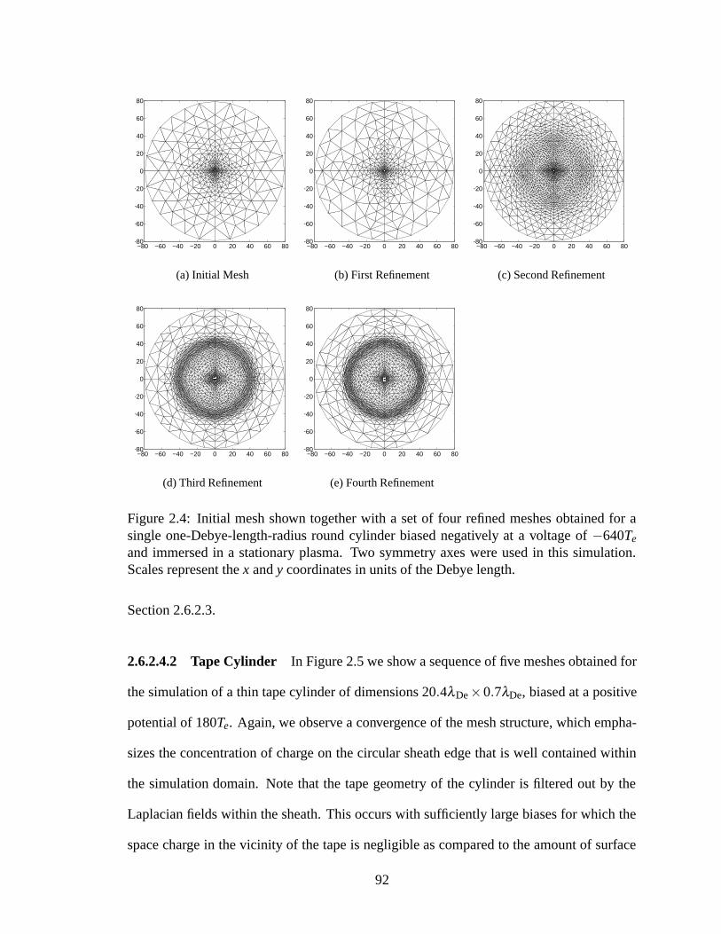
−80 −60 −40 −20 0 20 40 60 80−80
−60
−40
−20
0
20
40
60
80
(a) Initial Mesh
−80 −60 −40 −20 0 20 40 60 80−80
−60
−40
−20
0
20
40
60
80
(b) First Refinement
−80 −60 −40 −20 0 20 40 60 80−80
−60
−40
−20
0
20
40
60
80
(c) Second Refinement
−80 −60 −40 −20 0 20 40 60 80−80
−60
−40
−20
0
20
40
60
80
(d) Third Refinement
−80 −60 −40 −20 0 20 40 60 80−80
−60
−40
−20
0
20
40
60
80
(e) Fourth Refinement
Figure 2.4: Initial mesh shown together with a set of four refined meshes obtained for asingle one-Debye-length-radius round cylinder biased negatively at a voltage of −640Te
and immersed in a stationary plasma. Two symmetry axes were used in this simulation.Scales represent the x and y coordinates in units of the Debye length.
Section 2.6.2.3.
2.6.2.4.2 Tape Cylinder In Figure 2.5 we show a sequence of five meshes obtained for
the simulation of a thin tape cylinder of dimensions 20.4λDe×0.7λDe, biased at a positive
potential of 180Te. Again, we observe a convergence of the mesh structure, which empha-
sizes the concentration of charge on the circular sheath edge that is well contained within
the simulation domain. Note that the tape geometry of the cylinder is filtered out by the
Laplacian fields within the sheath. This occurs with sufficiently large biases for which the
space charge in the vicinity of the tape is negligible as compared to the amount of surface
92

−60 −40 −20 0 20 40 60−60
−40
−20
0
20
40
60
(a) Initial Mesh
−60 −40 −20 0 20 40 60−60
−40
−20
0
20
40
60
(b) First Refinement
−60 −40 −20 0 20 40 60−60
−40
−20
0
20
40
60
(c) Second Refinement
−60 −40 −20 0 20 40 60−60
−40
−20
0
20
40
60
(d) Third Refinement
−60 −40 −20 0 20 40 60−60
−40
−20
0
20
40
60
(e) Fourth Refinement
Figure 2.5: Initial mesh shown together with a set of four refined meshes obtained for atape cylinder with a width of 20.4λDe and a thickness of 0.7λDe. The tape was biased at apositive voltage of 180Te and immersed in a stationary plasma. Two symmetry axes wereused in this simulation. Scales represent the x and y coordinates in units of the Debyelength.
charge on the conducting tape itself.
2.6.2.4.3 Two Round Cylinders In Figure 2.6 we show a sequence of five meshes per-
taining to the 2-wire configuration. Two parallel one-Debye-length-radius round cylinders
are spaced 10λDe apart (center-to-center distance) and are both biased at a negative voltage
of −320Te. Here again, mesh convergence is observed after the fifth refinement step. De-
spite the asymmetric geometry of the structure, a circular charge-rich sheath structure still
forms on a circle of radius ∼ 30λDe and is resolved by the mesh refinement procedure.
93
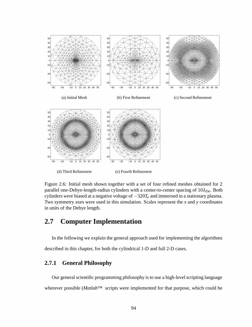
−50 −30 −10 0 10 20 30 40 50
−50
−30
−10
0
10
20
30
40
50
(a) Initial Mesh
−50 −30 −10 0 10 20 30 40 50
−50
−30
−10
0
10
20
30
40
50
(b) First Refinement
−50 −30 −10 0 10 20 30 40 50
−50
−30
−10
0
10
20
30
40
50
(c) Second Refinement
−50 −30 −10 0 10 20 30 40 50
−50
−30
−10
0
10
20
30
40
50
(d) Third Refinement
−50 −30 −10 0 10 20 30 40 50
−50
−30
−10
0
10
20
30
40
50
(e) Fourth Refinement
Figure 2.6: Initial mesh shown together with a set of four refined meshes obtained for 2parallel one-Debye-length-radius cylinders with a center-to-center spacing of 10λDe. Bothcylinders were biased at a negative voltage of−320Te and immersed in a stationary plasma.Two symmetry axes were used in this simulation. Scales represent the x and y coordinatesin units of the Debye length.
2.7 Computer Implementation
In the following we explain the general approach used for implementing the algorithms
described in this chapter, for both the cylindrical 1-D and full 2-D cases.
2.7.1 General Philosophy
Our general scientific programming philosophy is to use a high-level scripting language
wherever possible (Matlab™ scripts were implemented for that purpose, which could be
94

easily ported to functionally similar platforms such as Scilab or Octave), because it speeds
up development time and is less error prone. Where necessary, specific routines can then be
optimized through a different implementation using a lower-level language such as Fortran
90, a very standard platform in the scientific computing community. Appropriate interfaces
must then be used to dynamically link the Fortran 90 routines with Matlab™ at run time
when called from high-level Matlab™ scripts. Building Matlab™ EXecutable (MEX)
files using Fortran routines allows such interfacing.
2.7.2 Optimizing & Parallelizing the Vlasov Solver
At the early stages of development, it soon became apparent that the Vlasov solvers
(both 1-D and 2-D versions) were so computationally demanding that they required opti-
mization for any practical use.
The numerous numerical integrations performed in the 1-D Vlasov solver can actu-
ally be performed from within Matlab™, but it is much more efficient to implement the
numerical quadrature in Fortran 90.
In the case of the 2-D Vlasov solver, the computational requirements are much more
severe for the following three reasons in decreasing order of importance:
1. in KiPS-2D, each sample of the velocity distribution function that is being integrated
as part of the quadrature integration involves tracking a particle trajectory through the
potential structure, whereas in the case of KiPS-1D no particle tracking is required;
2. in KiPS-2D, the numerical quadrature integrations need to be performed in 2-D
velocity space, whereas in KiPS-1D one of the integrals is performed analytically,
which means that only a single-variable quadrature is required;
3. in KiPS-2D, the number of density samples that need to be computed, using numeri-
cal quadrature, is an order of magnitude larger than that which is required in the 1-D
95

implementation (∼ N2 as compared to N).
For these reasons, implementing a Vlasov solver that would be both efficient and accurate
mandated the use of parallel computing resources. To accomplish this, the 2-D version of
the Vlasov solver was thus implemented in Fortran 90 using an MPMD10 parallel process-
ing scheme based on the Parallel Virtual Machine library [32]. Since the Vlasov solver
consists of computing a fixed number (say M) of plasma density samples throughout the
computational domain based on a given potential profile, it can be divided easily into M
independent sub-tasks. These sub-tasks can be distributed to the slave nodes on a parallel
platform in what constitutes a coarse-grained parallel algorithm.
2.7.3 Present Parallel Computing Platform
The primary computing platform that we have used for this purpose consists of:
• A Linux-based master node,11 running the top-level Matlab™ scripts, the Matlab™-
based Poisson solver, and the top-level part of the Fortran 90-based Vlasov solver that
distributes sub-tasks to slave nodes.
• A dynamically-configured pool of about 150 Sun Blade 1000/1500 workstations,
each running a Fortran 90-based slave node and forming part of the Vlasov solver. A
total of 250 workstations are being used on an opportunistic basis, being swapped in
and out of the 150-workstation slave node pool according to their availability.12
2.7.4 Alternative Parallel Computing Platforms
Other parallel computing platforms were used as part of this project:
10Multiple Program, Multiple Data.11Dual-CPU Intel-based system running at a clock speed of 2.4 GHz with 4 GB of random-access memory.12A workstation is removed from the slave node pool when a console user logs in, and only moved back in
when no console users are logged in.
96

• An opportunistic pool of around 10 to 20 Linux workstations (based on 3.0-GHz
CPU’s) was used. Although the computing power of these nodes surpassed that of
the Sun Blade workstations, the number of Linux nodes accessible on campus could
not rival the shear number of existing Sun workstations;
• Dedicated Linux clusters, such as those operated by the University of Michigan’s
Computer Aided Engineering Network (CAEN) as part of the National Partnership
for Advanced Computer Infrastructure (NPACI), were used and shown to provide
very efficient computing power due to a better interconnection speed between the
slave and master nodes. However, the number of nodes and level of availability of
these queue-managed systems could not compare to that provided by the opportunis-
tic pooling of workstations for purposes of developing the code. Future production
runs requiring less user interaction and changes may be more suited for this kind of
platform.
Ultimately, the ideal computing platform is a dedicated Linux cluster comprised of
about 20 dual-CPU nodes. This would provide simulation times on par with our present
pool of 150 Sun workstations with a much higher degree of availability than pooled parallel
computing resources.
97
CHAPTER 3
Experimental Investigation of Electron-Collecting TetherSamples in a Mesosonic Xenon Plasma
3.1 Background
In this chapter, we present the results of an experimental investigation of the electron
current collection to tether samples of various cross-section geometries: round cylinder,
solid tape and slotted tape. These results were submitted for publication [71]. A compar-
ison of some of these results with kinetic simulation results obtained using KiPS-2D are
performed in Chapter 4 as part of the kinetic model validation.
The orbital-motion limit will be used as a baseline to compare the current collection
results for the various sample geometries and sizes. Recall that the OML electron current
collected by a thin cylinder is given by (1.8), which we re-write here for clarity:
I = Apnee
√eTe
2πme︸ ︷︷ ︸Ithe
{2√
π
√V0−Vp
Te+ exp
(V0−Vp
Te
)erfc
(√V0−Vp
Te
)}, (3.1)
with erfc(x) = 2√π∫ ∞
x e−t2dt. (3.1) is approximated, for V0−Vp > 2Te, by
I = Apnee
√eTe
2πme︸ ︷︷ ︸Ithe
2√
π
√1+
V0−Vp
Te, (3.2)
where V0 is the applied voltage, Vp is the plasma potential, Te is the electron temperature in
eV, Ap is the cylinder area, and Ithe is the electron thermal current given as a function of the
98

electron number density ne (in m−3), electron mass me, and electron charge magnitude e. In
an effort to facilitate comparisons with OML theory, results are presented in a normalized
format, showing the normalized current In = I/Ithe as a function of the normalized voltage
φ0 = (V0−Vp)/Te, which in the case of OML yields the simple equation:
In =2√
π√
φ0+ exp(φ0)erfc(√
φ0
)≈
2√
π√
1+φ0 . (3.3)
For large voltages, (3.3) is independent of the temperature Te, since both the right-hand side
and left-hand side are then proportional to 1/√
Te. This normalization allows us to directly
compare the OML theory, which only applies to thin cylinders in stationary plasmas, with
our experimental results involving a flowing plasma and various tether geometries.
In a previous investigation [72], it was concluded that tape tethers with widths up to
10 Debye lengths would perform close to an equal-area reference cylinder and that the
perpendicular tape orientation, with respect to plasma flow, would consistently outperform
the parallel orientation in terms of collected current.
In this chapter, we describe the results of a new set of chamber tests that were in-
tended to address questions of end effects and plasma source current limitations discussed
by Gilchrist et al [72], in addition to testing a larger breadth of “solid tape” widths and
a new “slotted tape” geometry with various porosities. The issue of end effects was ad-
dressed by adding guards to the tether samples, which are described below. The question
of possible plasma source current limitations, raised by Gilchrist et al [72], was resolved
by modifying the plasma source parameters, as discussed in Section 3.3.
3.2 Design and Assembly of Solid and Slotted Tape TetherGuarded Samples
The tether samples tested here, in addition to a thin cylindrical reference sample, in-
cluded solid tape samples in three different widths, and slotted samples of equivalent widths
99
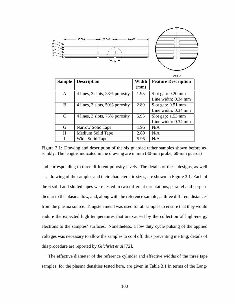
Sample Description Width Feature Description(mm)
A 4 lines, 3 slots, 28% porosity 1.95 Slot gap: 0.20 mmLine width: 0.34 mm
B 4 lines, 3 slots, 50% porosity 2.89 Slot gap: 0.51 mmLine width: 0.34 mm
C 4 lines, 3 slots, 75% porosity 5.95 Slot gap: 1.53 mmLine width: 0.34 mm
G Narrow Solid Tape 1.95 N/AH Medium Solid Tape 2.89 N/AI Wide Solid Tape 5.95 N/A
Figure 3.1: Drawing and description of the six guarded tether samples shown before as-sembly. The lengths indicated in the drawing are in mm (30-mm probe, 60-mm guards)
and corresponding to three different porosity levels. The details of these designs, as well
as a drawing of the samples and their characteristic sizes, are shown in Figure 3.1. Each of
the 6 solid and slotted tapes were tested in two different orientations, parallel and perpen-
dicular to the plasma flow, and, along with the reference sample, at three different distances
from the plasma source. Tungsten metal was used for all samples to ensure that they would
endure the expected high temperatures that are caused by the collection of high-energy
electrons to the samples’ surfaces. Nonetheless, a low duty cycle pulsing of the applied
voltages was necessary to allow the samples to cool off, thus preventing melting; details of
this procedure are reported by Gilchrist et al [72].
The effective diameter of the reference cylinder and effective widths of the three tape
samples, for the plasma densities tested here, are given in Table 3.1 in terms of the Lang-
100
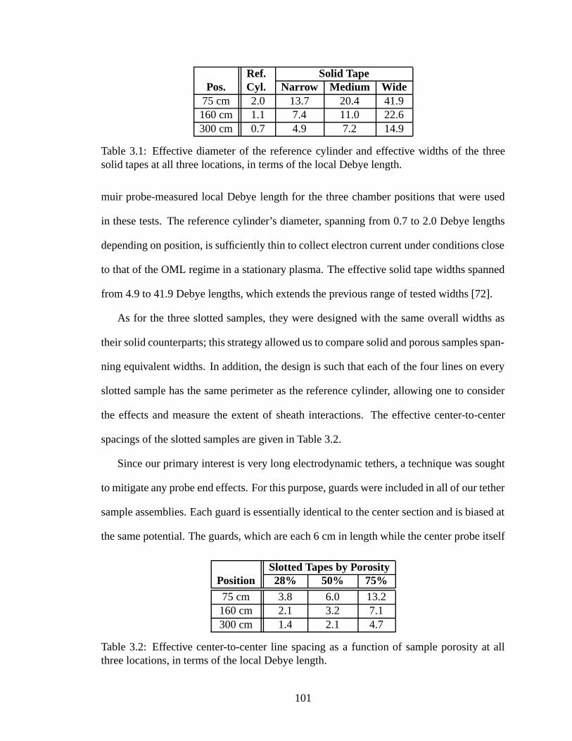
Ref. Solid TapePos. Cyl. Narrow Medium Wide
75 cm 2.0 13.7 20.4 41.9160 cm 1.1 7.4 11.0 22.6300 cm 0.7 4.9 7.2 14.9
Table 3.1: Effective diameter of the reference cylinder and effective widths of the threesolid tapes at all three locations, in terms of the local Debye length.
muir probe-measured local Debye length for the three chamber positions that were used
in these tests. The reference cylinder’s diameter, spanning from 0.7 to 2.0 Debye lengths
depending on position, is sufficiently thin to collect electron current under conditions close
to that of the OML regime in a stationary plasma. The effective solid tape widths spanned
from 4.9 to 41.9 Debye lengths, which extends the previous range of tested widths [72].
As for the three slotted samples, they were designed with the same overall widths as
their solid counterparts; this strategy allowed us to compare solid and porous samples span-
ning equivalent widths. In addition, the design is such that each of the four lines on every
slotted sample has the same perimeter as the reference cylinder, allowing one to consider
the effects and measure the extent of sheath interactions. The effective center-to-center
spacings of the slotted samples are given in Table 3.2.
Since our primary interest is very long electrodynamic tethers, a technique was sought
to mitigate any probe end effects. For this purpose, guards were included in all of our tether
sample assemblies. Each guard is essentially identical to the center section and is biased at
the same potential. The guards, which are each 6 cm in length while the center probe itself
Slotted Tapes by PorosityPosition 28% 50% 75%
75 cm 3.8 6.0 13.2160 cm 2.1 3.2 7.1300 cm 1.4 2.1 4.7
Table 3.2: Effective center-to-center line spacing as a function of sample porosity at allthree locations, in terms of the local Debye length.
101

Vacuum Epoxyat all joints
CIRCULARCERAMIC TUBING
outer dia: 0.64 mmInner dia: 0.3 mm
6 cm
3 cm
6 cm
Probe connector(SHV)
8 cm
Tungsten wire0.28 mm dia
Guard connector(SHV)
(a) Reference Cylinder
Vacuum Epoxyat all joints
CIRCULARCERAMIC TUBING
outer dia: 0.64 mmInner dia: 0.3 mm
6 cm
3 cm
6 cm
8 cm
Tungsten wire0.28 mm dia
OVAL CERAMIC TUBING
Tungsten Tape, Solid or Slotted
Probe connector(SHV)
Guard connector(SHV)
(b) Tape
Figure 3.2: Assemblies of the reference cylinder (a) and tape (b) guarded tether samples.
is 3 cm long, are shown in Figures 3.1 and 3.2 together with the probes. The effect of the
guards is to extend the cylindrical sheath to the full length of the sample, that is, five times
the length of the center probe on which current is measured.
Schematics of the full assemblies of the guarded tether samples are shown in Figure 3.2.
Due to the very small thickness of the tungsten samples under consideration here (0.1-mm
thick), it was not physically possible to feed the center probe using a feeding wire that
would have been inserted in one of the guards, as is typically done on some larger tri-
axial Langmuir probes. Instead, the center feed wire runs through an oblique ceramic tube
and connects to the center probe at one of its ends. On all samples, the feed wires to
both the guards and the probe were both soldered to the center conductor of a bulk-head
SHV (safe high voltage) connector; the connector-sample interfaces were then covered
102

Figure 3.3: Example of the ceramic attachment used on all solid and slotted tape samplesto attach the probe and guards while preserving electrical isolation.
with vacuum epoxy. The aluminum support structure for the SHV connectors provided a
localized ground.
The probe and guards also had to be physically attached but electrically insulated from
each other. Ceramic joints were used to this effect, an example of which is shown in Fig-
ure 3.3, and were attached to the tungsten probes and guards using stainless-steel machine
screws that were then carefully sanded down into a flat surface, in order to best emulate
the surface of the sample. The portion of the surface area of the ceramic joint covering the
tungsten probe and not covered by the screw head was accounted for in the calculation of
the total area of each probe.
Figure 3.4 shows pictures of three of our tether sample assemblies: the reference cylin-
der, the wide solid tape, and the 75%-porous wide slotted tape. The solid and slotted sam-
ples are shown with both SHV connectors installed, while the reference cylinder sample is
shown prior to the installation of the connectors.
103

(a)
(b)
(c)
Figure 3.4: Pictures of three typical tether samples: (a) the 0.28 mm-diameter referencecylinder, (b) the 5.95-mm wide solid tape, and (c) the 75%-porous wide slotted tape.
104

3.3 Vacuum Chamber Setup and Plasma Source Charac-teristics
The vacuum chamber tests were performed in the Large Vacuum Test Facility (LVTF), a
9-meter by 6-meter cylindrical stainless-steel-clad tank located within the Plasmadynamics
and Electric Propulsion Laboratory at the University of Michigan. For this experiment,
four of the seven available nude cryopumps were used to reach a high vacuum.
Figure 3.5 shows a diagram of the experimental setup within the LVTF. Two positioning
tables were used to change the separation distance between the thruster and sample plane
and to locate the sample under test directly along the thruster’s centerline. The thruster was
mounted on an x-y table that could move axially over a 1.0-m range and over sufficient ra-
dial range to cover all samples. The samples were mounted on an aluminum frame that was
connected to an axial table that could span a 1.5-m axial range. Combined table movement
allowed thruster–sample separation distance to change from 0.75 m to 3 m; our tests were
performed at 0.75 m, 1.60 m and 3.00 m from the thruster. Changing separation distance
was the primary mechanism for changing the plasma density seen at the sample plane.
Figure 3.6 shows an overall picture of the aluminum structure supporting the tether
samples and Langmuir probes, together with the Hall thruster used as a plasma source. The
latter is a 5 kW-class Hall thruster named “P5”, which was developed by the Plasmadynam-
ics and Electric Propulsion Laboratory and the Air Force Research Laboratory; more detail
is given by Haas et al. [73]. For these tests, the thruster was set at off-nominal conditions in
order to lower the plasma velocity and density seen along the thruster’s axial direction. Its
operating conditions are given in Table 3.3. The primary changes in those settings from the
ones used previously [72] are the discharge current, which was raised to 12.5 A, up from
5.3 A and 4 A and, consequently, the anode flow rate, which had to be raised to 112.1 sccm
to support the increased discharge current.
105

6 m
9 m
Langmuir probes
Samplesundertest
x
y
z
P5thrusterx-y table
axialtable
1.5 m
1.0 m
~0.75 m
Figure 3.5: Experimental setup in the Large Vacuum Test Facility (LVTF) at the Plasma-dynamics and Electric Propulsion Laboratory (PEPL).
Assessment of the emitted beam energy was estimated using two different techniques.
Laser-induced fluorescence (LIF) measurements have provided an estimate of 43 eV [74],
whereas Langmuir probe (LP) measurements in the ion saturation regime (discussed in
Appendix F) have yielded a value of 25.0 eV. More detail regarding the LIF measurements
is given by Gilchrist et al [72] and Williams et al [75]. It should be noted that the LP value
of 25.0 eV is close to, if not within, the bounds of the error on the LIF-determined beam
energy value, which is about 40%, given that the reported typical error on the velocity
106
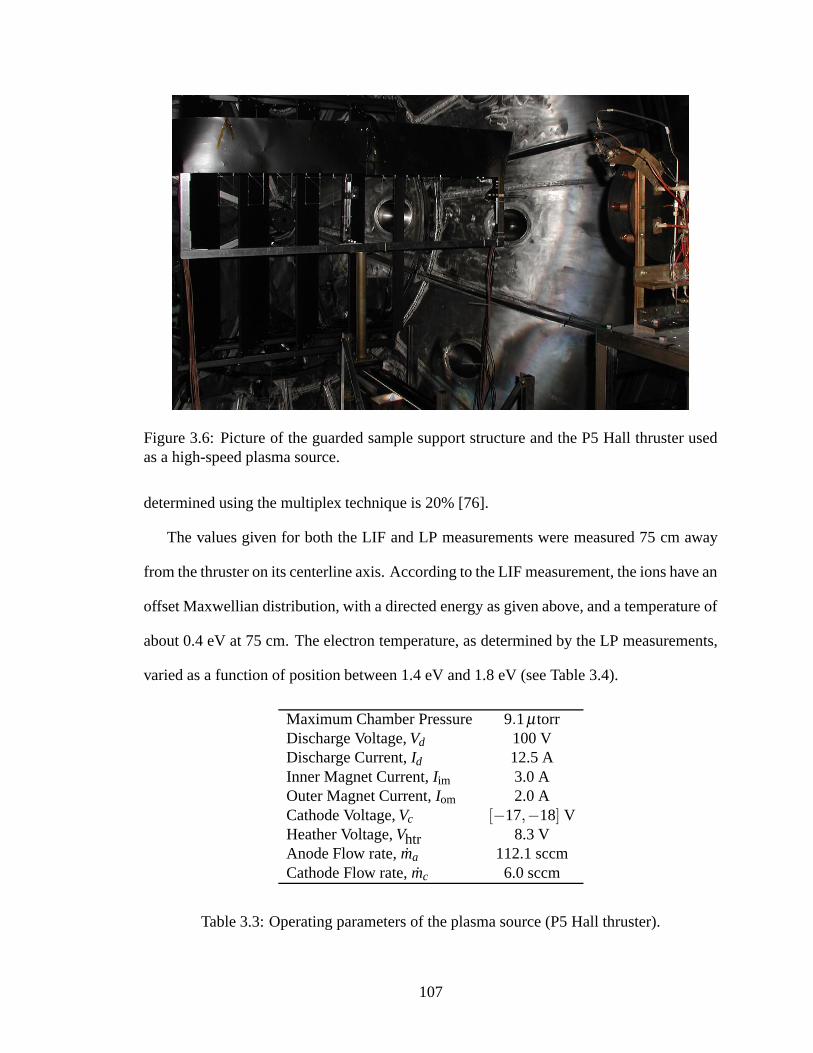
Figure 3.6: Picture of the guarded sample support structure and the P5 Hall thruster usedas a high-speed plasma source.
determined using the multiplex technique is 20% [76].
The values given for both the LIF and LP measurements were measured 75 cm away
from the thruster on its centerline axis. According to the LIF measurement, the ions have an
offset Maxwellian distribution, with a directed energy as given above, and a temperature of
about 0.4 eV at 75 cm. The electron temperature, as determined by the LP measurements,
varied as a function of position between 1.4 eV and 1.8 eV (see Table 3.4).
Maximum Chamber Pressure 9.1 µtorrDischarge Voltage, Vd 100 VDischarge Current, Id 12.5 AInner Magnet Current, Iim 3.0 AOuter Magnet Current, Iom 2.0 ACathode Voltage, Vc [−17,−18] VHeather Voltage, Vhtr 8.3 VAnode Flow rate, ma 112.1 sccmCathode Flow rate, mc 6.0 sccm
Table 3.3: Operating parameters of the plasma source (P5 Hall thruster).
107

ne Te λDe µb
Position (m−3) (eV) (mm)
75 cm 4.95×10¹⁵ 1.80 0.14 95%160 cm 1.37×10¹⁵ 1.72 0.26 53%300 cm 0.51×10¹⁵ 1.47 0.40 32%
Table 3.4: Variation of the measured plasma parameters as a function of distance fromthe Hall thruster. Measurements were performed using the ion saturation and electronretardation data from a transverse LP. The beam energy value determined using the LP is25 eV. The “beam fraction”, µb, indicates the fraction of all ions that are believed to bebeam (high-speed) ions. Density, temperature and Debye length estimates have about 6%,1% and 3.5% accuracy, as discussed in F.1.
A schematic of the current–voltage measurement system is given in Figure 3.7. We
connected a Universal Voltronics BRC 20 000 HV power supply to the tether samples
through a high-voltage relay box inside the chamber. The HV power supply was controlled
via RS–232 by the computer controller running a custom virtual instrument (VI) under
LabVIEWTM. The computer commanded the HV power supply to a specified voltage and
then quickly back to zero (within 50 to 100 ms), followed by several seconds of cool-down
to minimize sample heating. Current measurement on the sample probes was achieved
using an American Aerospace Controls 835–2–10 current sensor; increased current sensi-
tivity was obtained by looping the HV supply line ten times through the sensor. The current
to the sample guards was measured separately using a F.W. Bell ma-2000 current sensor.
An HP 34970 data acquisition unit was used to measure the voltage signals generated by
both current sensors. The data were recorded as triplets containing the applied voltage, the
probe current, and the guard current.
3.4 Plasma Parameter Measurements Using Negatively-Biased Langmuir Probes
Plasma density, temperature, flow speed, and the fraction of beam ions to background
ions were determined using a 4-cm long, vertically oriented (i.e., perpendicular to the flow)
108

Electrometer
Computer ControllerIEEE-488
To Langmuir Probes
High Voltage Power Supply
AACCurrent Probe
Data Acquisition Unit
High VoltageSwitch Box
To Samples
10 Loops
RS-232
Chamber Wall
Switch BoxControl
FWBell CurrentSensor
To Guards
Figure 3.7: Schematic of the computer-controlled high-voltage test equipment setup.
Langmuir Probe (LP) with a diameter of 0.28 mm (same diameter as for the reference
cylinder sample). All LP sweeps were performed using a Keithley 2410 source electrometer
controlled via a custom LabVIEWTM script running on a personal computer.
The plasma parameters, shown in Table 3.4, were extracted from the ion saturation
(OML regime) and electron retardation regions of the I–V characteristics using a LP ori-
ented transverse to the direction of the flow. In the OML regime, there are several ad-
vantages to selecting the ion saturation as opposed to the electron saturation region for
parameter extraction. A cylindrical probe oriented transverse to the flow in a high-speed
plasma is known to be virtually free of end effects [39]. In addition, a simple but fairly
accurate collection model is available that accounts for the velocity of the flow in that
regime [29]. By contrast, there are currently no accurate models for the electron collec-
tion to an electron-attracting probe that can account for the plasma flow. In the mesosonic
regime, where the plasma flow is much faster than the thermal ion velocity yet much smaller
than the electron thermal velocity, important sheath asymmetries and elongations exist in
109

the electron-attracting mode that get stronger with the applied bias, which makes this a
complex problem. One of the aims of the experimental work presented here is in fact to
improve the understanding of the macroscopic effect of plasma flow on electron collection.
Finally, using a negatively-biased LP provides an independent assessment of the plasma
parameters, since all the test samples are biased positively.
The procedure that was used for the plasma parameter extraction from the Langmuir
probe current characteristics is detailed in Appendix F. In addition to providing plasma
density and temperature readings, this analysis quantifies the ion “beam fraction” and de-
scribes what appears to be effective workfunction variations.
The results of this analysis indicate the existence of a population of thermal ions far
from the high-speed plasma source, which is born out of cumulative charge-exchange col-
lisions between the incident high-speed ions and the neutral background xenon gas. The
number-density ratio of high-speed ions to thermal ions is quantified in Table 3.4 and ranges
from an assumed 95% at the closest distance (75 cm) to a calculated 32% at the farthest dis-
tance (300 cm). This fall-off of the fraction of beam ions can be best-fitted to an equivalent
“beam ion survival characteristic distance” of 2.14 m, which is just short of the theoretical
charge-exchange mean free path of 2.6 m corresponding to the measured background pres-
sure, ion energy, and assuming a background neutral temperature of 350 K. The fall-off is
likely due to a combination of effects, such as the beam loss through charge-exchange col-
lisions and the geometrical divergence of the beam, which may explain the smaller value
obtained.
3.5 Experimental Results & Analysis
Our results are presented here in four parts: the reference cylinder, the solid tapes, the
slotted tapes, and, finally, a comparison of the solid and slotted tapes. All results are pre-
110

sented in normalized form. The collected current is normalized to the electron thermal
current Ithe collected at the plasma potential, as defined in (3.1). All probes should collect
this amount of current when biased at the plasma potential. The normalization of potential
consists of a translation corresponding to the plasma potential, followed by a scaling by the
inverse of the electron temperature, Te. An OML theoretical plot, scaled this way, would
result in (3.3) and would be independent of temperature, as discussed in the introduction.
This normalization provides a means of evaluating the performance of various probes by
comparing them to OML theory as well as by comparing their respective “electron collec-
tion efficiencies.” Note, however, that the extent of the normalized voltage axis varies from
one graph to another, due to changes in the electron temperature used in the normalization
of this axis, and from variations in the collected data range.
3.5.1 Reference Cylinder
Figure 3.8 shows the normalized results for the reference cylinder at the three distances
from the plasma source (Figure 3.9 shows identical information for the reference cylinder).
The reference cylinder at 75 cm is seen to collect much more current than that predicted by
OML theory, by as much as 40% at a bias of 100 Te. This enhancement is seen to decrease
as we move away from the thruster to 160 cm and 300 cm. In fact, there is no enhancement
at 300 cm. Since the fraction of beam ions was also determined to fall off with distance
(95% at 75 cm, 53% at 160 cm, and 32% at 300 cm), this observed enhancement could be
linked to the effects of the high-speed flow. This change in enhancement level is most likely
not due to the change in the effective size of the reference cylinder (2.0, 1.1, and 0.7 Debye
lengths) since decreasing the size would theoretically have the opposite effect, that is, to
increase the collection efficiency rather than to decrease it as observed here. In addition,
even if there were any residual end effects despite the use of our guard structures, we
111
believe that the enhancement could not be attributed to those end effects, since the stronger
end effects should occur at the location where the cylinder is the shortest in terms of the
local Debye length (at 300 cm), whereas the observed enhancement is strongest where the
effective cylinder length is the longest (at 75 cm).
3.5.2 Solid Tapes
Figure 3.8 presents results for all solid tape samples and the reference cylinder at all
three distances from the plasma source (75 cm, 160 cm, and 300 cm). The effective tape
widths, shown in terms of the Debye lengths in the legend as well as in Table 3.1, span
from 4.9 to 41.9 electron Debye lengths. Three major observations are noted from these
results:
1. All samples collect electrons less efficiently than the reference cylinder, as is ex-
pected because of their larger sizes. Likewise, all samples are seen to collect less
efficiently as the effective width of the tape is increased, regardless of their orienta-
tion. This is true whether we are looking at a mostly high-speed plasma (at 75 cm)
or a mostly quiescent plasma (at 300 cm). When compared to the reference cylin-
der, the relative collection efficiency of all solid tapes decreases with increasing tape
width, similar to the “current ratio” characteristic reported by Estes et al [12, Figure
4(b)] based on an effective circular cylinder radius equal to four times the tape width
(Req = 4wtape [11]). The overall relative efficiency is seen to be somewhat lower than
that predicted by Estes and Sanmartın [12] and is closer to, although still lower than,
our steady-state kinetic simulation results (see Chapter 4). This reduced efficiency
may be explained by the reduction in collection efficiency due to the presence of
mounting screws that account for a small fraction of the total collecting area.
2. At both the 75-cm and 160-cm distances, all solid tape samples collected more cur-
112

0 20 40 60 80 1000
2
4
6
8
10
12
14
16
18
φ0=(V
0−V
p)/T
e
I / (
Ap I th
e)
Normalized Current Characteristics of Solid Samples at 75 cm
n=5 × 10¹⁵ m−3, Te=1.8 eV, µ
b≈95 %
Reference Cylinder, dia=0.28mm=2.0 λdeParal. Solid Tape, width=1.95 mm=13.7 λdeParal. Solid Tape, width=2.89mm=20.4 λdeParal. Solid Tape, width=5.95mm=41.9 λdePerp. Solid Tape, width=1.95 mm=13.7 λdePerp. Solid Tape, width=2.89mm=20.4 λdePerp. Solid Tape, width=5.95mm=41.9 λdeTheory: Retardation and OMLElectron Thermal Current
0 20 40 60 80 100 120 1400
2
4
6
8
10
12
14
16
18
φ0=(V
0−V
p)/T
e
I / (
Ap I th
e)
Normalized Current Characteristics of Solid Samples at 160 cm
n=1.4 × 10¹⁵ m−3, Te=1.7 eV, µ
b≈53 %
Reference Cylinder, dia=0.28mm=1.1 λdeParal. Solid Tape, width=1.95 mm=7.4 λdeParal. Solid Tape, width=2.89mm=11.0 λdeParal. Solid Tape, width=5.95mm=22.6 λdePerp. Solid Tape, width=1.95 mm=7.4 λdePerp. Solid Tape, width=2.89mm=11.0 λdePerp. Solid Tape, width=5.95mm=22.6 λdeTheory: Retardation and OMLElectron Thermal Current
(a) (b)
0 20 40 60 80 100 120 140 1600
2
4
6
8
10
12
14
16
φ0=(V
0−V
p)/T
e
I / (
Ap I th
e)
Normalized Current Characteristics of Solid Samples at 300 cm
n=5.1 × 10¹⁴ m−3, Te=1.5 eV, µ
b≈32 %
Reference Cylinder, dia=0.28mm=0.7 λdeParal. Solid Tape, width=1.95 mm=4.9 λdeParal. Solid Tape, width=2.89mm=7.2 λdeParal. Solid Tape, width=5.95mm=14.9 λdePerp. Solid Tape, width=1.95 mm=4.9 λdePerp. Solid Tape, width=2.89mm=7.2 λdePerp. Solid Tape, width=5.95mm=14.9 λdeTheory: Retardation and OMLElectron Thermal Current
(c)
Figure 3.8: Normalized I–V characteristics of parallel and perpendicular solid tapes at (a)75 cm, (b) 160 cm and (c) 300 cm.
rent when oriented perpendicular (transverse) rather than parallel to the flow. In
addition, the contrast between perpendicular and parallel results is observed to get
stronger as the effective width of the tape increases. However, such a clear distinction
is not evident in the measurements taken at 300 cm, which is likely a consequence of
the low fraction of beam ions that was measured at that location, combined with the
lower effective widths of the tapes (the Debye length was highest at that location) as
compared to the two other locations. The near-overlapping of the perpendicular and
parallel results at 300 cm also serves as qualitative confirmation that the measured
113

fraction of beam ions has dropped down as compared to that measured at 75 cm.
3. The previous observation of the increase of collected current from parallel to perpen-
dicular is seen to occur when the probes are biased above a certain threshold, which
varies from about 25 to 40 volts. This level is on the order of the estimated ion beam
energy (somewhere between 25 eV, according to the LP results, and 43 eV, according
to the LIF results). At this threshold bias, the parallel results are seen to present a
“knee”, which is most apparent in the widest effective tape at 75 cm. These observa-
tions are in agreement with previous results based on a similar experiment [72].
3.5.3 Slotted Tapes
Figure 3.9 presents results for all slotted tape samples and the reference cylinder at
all three distances from the plasma source. The effective center-to-center line spacings,
shown in terms of the Debye lengths in the legend as well as in Table 3.2, span from 1.4
to 13.2 Debye lengths. It should be emphasized that the overall widths of the slotted tapes,
including the gap spacings, are the same as the solid tape widths (1.95 mm, 2.89 mm, and
5.95 mm). The following are some observations regarding these results:
• Similar to the tape results, the slotted samples collected electrons less efficiently,
on a per-area basis, than the reference cylinder at all three distances, although they
were more efficient than the solid tapes. This is an indication that the individual-line
sheaths were strongly interacting.
• The contrast between the results in the parallel and perpendicular orientations has a
similar character as that observed for the solid tapes: the perpendicular slotted tapes
collect more current than their parallel counterparts. However, distinct from the solid
tape results is the smaller variation between the responses of the three perpendicular
114

0 20 40 60 80 1000
2
4
6
8
10
12
14
16
18
I / (
Ap I th
e)
Normalized Current Characteristics of Slotted Samples at 75 cm
n=5 × 10¹⁵ m−3, Te=1.8 eV, µ
b≈95 %
φ0=(V
0−V
p)/T
e
Reference Cylinder, dia=0.28mm=2.0 λdeParal. Slotted Tape, Line Spacing=3.8 λdeParal. Slotted Tape, Line Spacing=6.0 λdeParal. Slotted Tape, Line Spacing=13.2 λdePerp. Slotted Tape, Line Spacing=3.8 λdePerp. Slotted Tape, Line Spacing=6.0 λdePerp. Slotted Tape, Line Spacing=13.2 λdeTheory: Retardation and OMLElectron Thermal Current
0 20 40 60 80 100 120 1400
2
4
6
8
10
12
14
16
18
φ0=(V
0−V
p)/T
e
I / (
Ap I th
e)
Normalized Current Characteristics of Slotted Samples at 160 cm
n=1.4 × 10¹⁵ m−3, Te=1.7 eV, µ
b≈53 %
Reference Cylinder, dia=0.28mm=1.1 λdeParal. Slotted Tape, Line Spacing=2.1 λdeParal. Slotted Tape, Line Spacing=3.2 λdeParal. Slotted Tape, Line Spacing=7.1 λdePerp. Slotted Tape, Line Spacing=2.1 λdePerp. Slotted Tape, Line Spacing=3.2 λdePerp. Slotted Tape, Line Spacing=7.1 λdeTheory: Retardation and OMLElectron Thermal Current
(a) (b)
0 20 40 60 80 100 120 140 1600
2
4
6
8
10
12
14
16
φ0=(V
0−V
p)/ T
e
I / (
Ap I th
e)
Normalized Current Characteristics of Slotted Samples at 300 cm
n=5.1 × 10¹⁴ m−3, Te=1.5 eV, µ
b≈32 %
Reference Cylinder, dia=0.28mm=0.7 λdeParal. Slotted Tape, Line Spacing=1.4 λdeParal. Slotted Tape, Line Spacing=2.1 λdeParal. Slotted Tape, Line Spacing=4.7 λdePerp. Slotted Tape, Line Spacing=1.4 λdePerp. Slotted Tape, Line Spacing=2.1 λdePerp. Slotted Tape, Line Spacing=4.7 λdeTheory: Retardation and OMLElectron Thermal Current
(c)
Figure 3.9: Normalized I–V characteristics of parallel and perpendicular slotted tapes at(a) 75 cm, (b) 160 cm and (c) 300 cm.
slotted tapes widths (especially at 75 cm and 160 cm) as compared to the parallel
slotted ones. Specifically, the efficiency of the widest (and most porous) slotted tape,
with a line spacing of 13.2 Debye lengths at 75 cm, is roughly on par with that of
the medium slotted tape (6.0 Debye lengths at 75 cm), and even goes above it at
the highest bias potentials. This may indicate that the widest line spacing was close
to a critical value, corresponding to the minimum efficiency, and beyond which the
collection efficiency would start increasing again, up to the very wide spacing limit
where all four lines become independent and collect as efficiently as the reference
115
cylinder. We seem to have attained this limit only in the perpendicular orientation,
which can be explained by the fact that the sheath elongations in the direction of the
flow [77,78] would cause the sheath interactions to grow stronger when aligned with
(i.e., parallel to) the flow, thereby moving the critical spacing to a higher value for
the parallel case. Clearly, testing of wider line spacings will be required to determine
those critical values and relate them to the flow energy.
• A “knee” is most apparent in the results for the widest parallel slotted tapes at 75 cm
and 160 cm, around 29 and 21 volts, respectively (note that the positions of the knees
on the graphs need to be scaled with their respective electron temperatures), which
is close to the estimated ion beam energy. The parallel and perpendicular results
separate at the potential bias corresponding to the location of this knee.
3.5.4 Comparison of the Solid and Slotted Tapes
Figs. 3.10–3.12 show the same sets of results shown earlier, but with the solid and
slotted tapes plotted on common graphs to facilitate their comparison. The absolute amount
of current collected by the solid tape samples was higher than that collected by the slotted
tape samples in all cases, as expected, and is not shown here. The slotted samples were
somewhat more efficient on a per-area basis than their solid counterparts. This is true at all
positions, and does not seem to be a function of the fraction of beam ions present. Hence,
the slotted samples are always more efficient on a per-area basis, regardless of whether in a
stationary or flowing plasma. For example, at 75 cm the parallel wide slotted tape collected
about 37% of the current collected by the parallel wide solid tape at a normalized bias of
80Te, a somewhat higher fraction than the porosity of the sample, which was 28%.
116

0 20 40 60 80 1000
2
4
6
8
10
12
φ0=(V
0−V
p)/T
e
I /(A
p I the)
Normalized Characteristics of Parallel Solid and Slotted Samples at 75 cm
n=5 × 10¹⁵ m−3, Te=1.8 eV, µ
b≈95 %
Paral. Solid Tape, width=1.95 mm=13.7 λdeParal. Solid Tape, width=2.89mm=20.4 λdeParal. Solid Tape, width=5.95mm=41.9 λdeParal. Slotted Tape, Line Spacing=3.8 λdeParal. Slotted Tape, Line Spacing=6.0 λdeParal. Slotted Tape, Line Spacing=13.2 λde
0 20 40 60 80 1000
2
4
6
8
10
12
φ0=(V
0−V
p)/T
e
I /(A
p I the)
Normalized Characteristics of Perpendicular Solid and Slotted Samples at 75 cm
n=5 × 10¹⁵ m−3, Te=1.8 eV, µ
b≈95 %
Perp. Solid Tape, width=1.95 mm=13.7 λdePerp. Solid Tape, width=2.89mm=20.4 λdePerp. Solid Tape, width=5.95mm=41.9 λdePerp. Slotted Tape, Line Spacing=3.8 λdePerp. Slotted Tape, Line Spacing=6.0 λdePerp. Slotted Tape, Line Spacing=13.2 λde
Figure 3.10: Comparison of the I–V characteristics of solid and slotted tapes at 75 cm.
117

0 20 40 60 80 100 120 1400
2
4
6
8
10
12
14
φ0=(V
0−V
p)/T
e
I /(A
p I the)
Normalized Characteristics of Parallel Solid and Slotted Samples at 160 cm
n=1.4 × 10¹⁵ m−3, Te=1.7 eV, µ
b≈53 %
Paral. Solid Tape, width=1.95 mm=7.4 λdeParal. Solid Tape, width=2.89mm=11.0 λdeParal. Solid Tape, width=5.95mm=22.6 λdeParal. Slotted Tape, Line Spacing=2.1 λdeParal. Slotted Tape, Line Spacing=3.2 λdeParal. Slotted Tape, Line Spacing=7.1 λde
0 20 40 60 80 100 1200
2
4
6
8
10
12
14
φ0=(V
0−V
p)/T
e
I /(A
p I the)
Normalized Characteristics of Perpendicular Solid and Slotted Samples at 160 cm
n=1.4 × 10¹⁵ m−3, Te=1.7 eV, µ
b≈53 %
Perp. Solid Tape, width=1.95 mm=7.4 λdePerp. Solid Tape, width=2.89mm=11.0 λdePerp. Solid Tape, width=5.95mm=22.6 λdePerp. Slotted Tape, Line Spacing=2.1 λdePerp. Slotted Tape, Line Spacing=3.2 λdePerp. Slotted Tape, Line Spacing=7.1 λde
Figure 3.11: Comparison of the I–V characteristics of solid and slotted tapes at 160 cm.
118

0 20 40 60 80 100 120 140 1600
2
4
6
8
10
12
14
φ0=(V
0−V
p)/T
e
I /(A
p I the)
Normalized Characteristics of Parallel Solid and Slotted Samples at 300 cm
n=5.1 × 10¹⁴ m−3, Te=1.5 eV, µ
b≈32 %
Paral. Solid Tape, width=1.95 mm=4.9 λdeParal. Solid Tape, width=2.89mm=7.2 λdeParal. Solid Tape, width=5.95mm=14.9 λdeParal. Slotted Tape, Line Spacing=1.4 λdeParal. Slotted Tape, Line Spacing=2.1 λdeParal. Slotted Tape, Line Spacing=4.7 λde
0 20 40 60 80 100 120 140 1600
2
4
6
8
10
12
φ0=(V
0−V
p)/T
e
I /(A
p I the)
Normalized Characteristics of Perpendicular Solid and Slotted Samples at 300 cm
n=5.1 × 10¹⁴ m−3, Te=1.5 eV, µ
b≈32 %
Perp. Solid Tape, width=1.95 mm=4.9 λdePerp. Solid Tape, width=2.89mm=7.2 λdePerp. Solid Tape, width=5.95mm=14.9 λdePerp. Slotted Tape, Line Spacing=1.4 λdePerp. Slotted Tape, Line Spacing=2.1 λdePerp. Slotted Tape, Line Spacing=4.7 λde
Figure 3.12: Comparison of the I–V characteristics of solid and slotted tapes at 300 cm.
119

3.6 Present Status and Conclusions
Several conclusions can be drawn from the analysis of these experimental results:
1. the plasma flow leads to significant current enhancements over that predicted by the
orbital-motion-limited theory;
2. the electron collection efficiency of solid tapes (on a per area basis) decreases as the
width of the tape is increased;
3. beyond a threshold bias close to the beam energy, solid and slotted tapes both collect
more current when oriented transverse (perpendicular) to the flow;
4. equivalent-width slotted tapes are more efficient electron collectors than solid tapes
on a per-area basis;
5. our data suggests the electron collection efficiency of slotted tapes decreases with
increasing line spacing until a possible minimum efficiency is attained, beyond which
it is expected to start increasing again. The minimum may have been attained in
the case of the samples oriented transverse to the flow, but not in the case of the
samples aligned with the flow, for which the critical spacing is likely higher due to
an increased sheath interaction radius of each line caused by the elongation of the
sheath associated with plasma flow.
Further experiments are needed to more completely quantify the observed effects. In
addition, larger line spacings should be tested in both the parallel and perpendicular ori-
entations to verify the existence of and quantify the critical spacing that corresponds to a
minimum collection efficiency.
A lower background pressure might help improve the survival of the ion beam out to 3
meters, and could possibly be achieved with the use of additional cryopumps. For example,
120

using 7 cryopumps instead of 4, we could expect a drop of the background pressure by a
factor 4/7, and consequently an increase of the charge-exchange mean-free-path length by
a factor 7/4. Since the value shown for the high-speed beam fraction (µb = 32%) at 300 cm
in Table 3.4 is consistent with a mean free path of about 2.6 meters, this additional pumping
power could be expected to increase the mean free path to 2.6 m×7/4≈ 4.6 m. This would
therefore improve the beam survival at 300 cm from 32% to 52% (exp(−3.0 m
4.6 m
)= 0.52).
Finally, in future experiments one should consider shifting the entire hardware setup
further away from the downstream end of the vacuum chamber, which might reduce a
possible accumulation of neutrals near that end of the chamber, since the cryopumps are
located on the upstream end.
121

CHAPTER 4
Simulation Results and Validation
In this chapter we present and analyze our simulation results, and proceed to validations
with other published results wherever possible. Section 4.1 describes the normalizations
used throughout this chapter. Section 4.2 discusses the simulation results applicable to a
round cylinder in a stationary plasma. Sections 4.3 and 4.4 discuss probe geometry effects
using simulation results pertaining to the two-wire and thin tape cylinder, respectively.
Finally, Sections 4.5 and 4.6 discuss the effects of plasma flow on sheath structure and
current collection for ion- and electron-attracting round cylinders.
Note that for all of the simulations presented in this chapter, the electron and ion pop-
ulations are at thermal equilibrium (Ti = Te), because this setting is most representative
of the ionospheric environments of interest. Although they were not tested as part of this
analysis of results, the model does allow for settings of the temperature ratio Ti/Te other
than 1.13
4.1 Definition of Normalized Physical Quantities
All simulation parameters and results are presented in a normalized form in order to
make them as general as possible. The normalizations used in this chapter are consistent
13Results shown in Ref. [8] indicate that, for temperature ratios Ti/Te below unity, we should expect areduction of the sheath dimensions as well as the collected ion current for ion-attracting bias potentials ascompared to the case where Ti = Te.
122

with those used to present our experimental results in normalized form in Chapter 3. The
following is a description of the normalized parameters used throughout this chapter:
• The number densities are normalized with respect to the number density of the back-
ground plasma (the ambient density). The normalized density nn is the ratio of the
actual density n (in m−3) to the background number density n0 of the plasma: nn=nn0
.
• Similarly, the net charge density is normalized in terms of the ambient density and
the electron charge e. At any location in space, the normalized net charge density ρn
is given by
ρn =ρ
en0=
ni−ne
n0, (4.1)
where ρ is the actual net charge density.
• The electric potentials are normalized in terms of the electron plasma temperature
Te (units of eV) and the plasma potential Vp (in volts). At any location in space the
normalized potential is thus given by
φ =V −Vp
Te, (4.2)
where V is the local electric potential and Vp is the background plasma potential. The
bias potential is similarly normalized according to φ0 =V0−Vp
Te, where V0 is the bias
potential in volts.
• All coordinates and dimensions are normalized in terms of the electron Debye length
in the ambient plasma. The normalized coordinates (xn,yn) are given by
xn =x
λDeand yn =
yλDe, (4.3)
where (x,y) are the physical coordinates and λDe is the electron Debye length, both
given in units of meters.
123
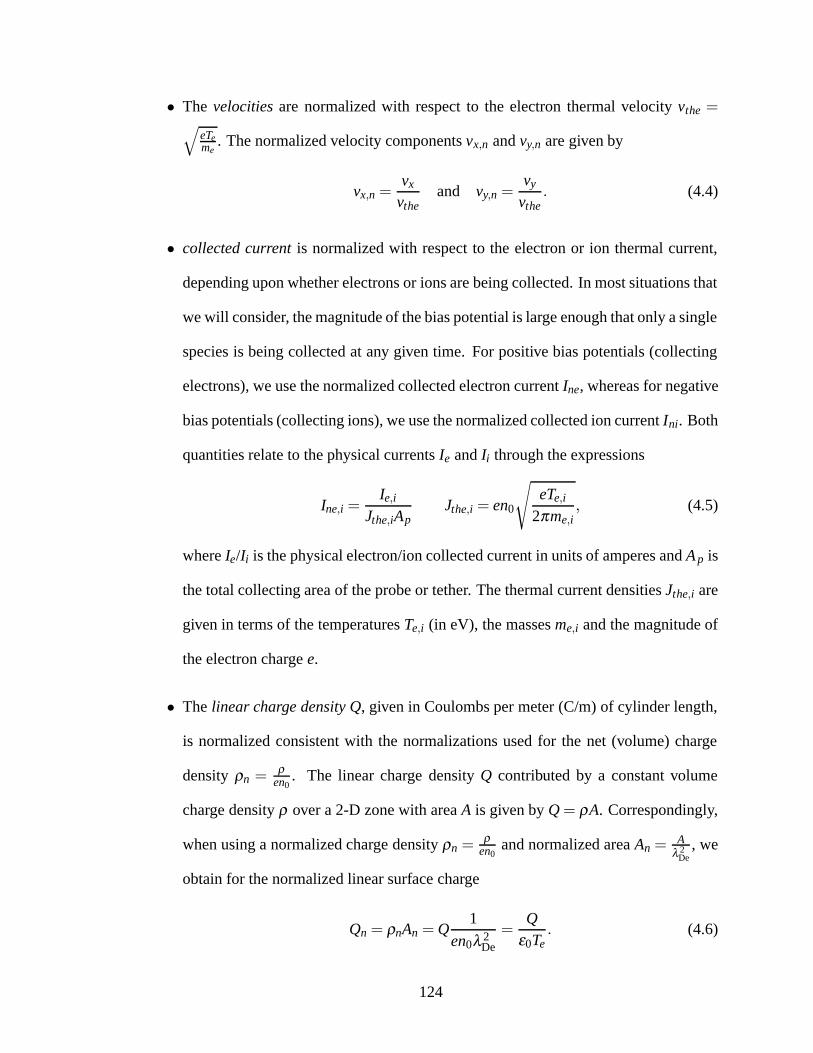
• The velocities are normalized with respect to the electron thermal velocity vthe =√eTeme
. The normalized velocity components vx,n and vy,n are given by
vx,n =vx
vtheand vy,n =
vy
vthe. (4.4)
• collected current is normalized with respect to the electron or ion thermal current,
depending upon whether electrons or ions are being collected. In most situations that
we will consider, the magnitude of the bias potential is large enough that only a single
species is being collected at any given time. For positive bias potentials (collecting
electrons), we use the normalized collected electron current Ine, whereas for negative
bias potentials (collecting ions), we use the normalized collected ion current Ini. Both
quantities relate to the physical currents Ie and Ii through the expressions
Ine,i =Ie,i
Jthe,iApJthe,i = en0
√eTe,i
2πme,i, (4.5)
where Ie/Ii is the physical electron/ion collected current in units of amperes and A p is
the total collecting area of the probe or tether. The thermal current densities Jthe,i are
given in terms of the temperatures Te,i (in eV), the masses me,i and the magnitude of
the electron charge e.
• The linear charge density Q, given in Coulombs per meter (C/m) of cylinder length,
is normalized consistent with the normalizations used for the net (volume) charge
density ρn =ρ
en0. The linear charge density Q contributed by a constant volume
charge density ρ over a 2-D zone with area A is given by Q= ρA. Correspondingly,
when using a normalized charge density ρn =ρ
en0and normalized area An =
Aλ 2
De, we
obtain for the normalized linear surface charge
Qn = ρnAn =Q1
en0λ 2De
=Q
ε0Te. (4.6)
124
• The ion and electron temperatures Ti and Te are normalized to the electron tempera-
ture Te, resulting in
Ti,n =Ti
Teand Te,n =
Te
Te= 1, (4.7)
which yields a trivial result of unity for the normalized electron temperature.
• The particle masses mi and me are normalized to the electron mass me, i.e.
mi,n =mi
meand me,n =
me
me= 1, (4.8)
which yields a trivial result for the normalized electron mass.
• Similar to the masses, the particle charges qi and qe are normalized to the electron
charge qe, i.e.
qi,n =qi
qeand qe,n =
qe
qe= 1. (4.9)
The normalizations above are consistent with the following normalization of Poisson’s
equation (2.5):
∇2V ≡d2Vdx2 +
d2Vdy2 =−
ρε0
⇐⇒ ∇2nφ ≡
d2φdx2
n+
d2φdy2
n=−ρn︸ ︷︷ ︸,normalized form (4.10)
where ρn ≡ρ
ε0Teand ∇n is the Laplacian applied on the normalized space coordinates
(xn,yn). In addition, Vlasov’s equation (2.9) can be recast in terms of the normalized
quantities:
vx,n∂ fn
∂xn+ vy,n
∂ fn
∂yn−
qn
mn
∂φ∂xn
∂ fn
∂vx,n−
qn
mn
∂φ∂yn
∂ fn
∂vy,n= 0, (4.11)
where fn, qn and mn are normalized quantities that apply to either electrons or ions, i.e.,
fn =
{fe/n0
fi/n0
}, qn =
{qe,n
qi,n
}, and mn =
{me,n
mi,n
}. (4.12)
Because both of the fundamental equations used in the computational model can be
recast in normalized form as given by (4.10) and (4.11), any solutions that we obtain based
125

on the simulations can be applied to a vast number of practical cases based on the proper
scaling of the normalized quantities using the physical values for the parameters n0, Te, me,
and qe.
4.2 Single Round Cylinder in Stationary Plasma
The most simple configuration that can be analyzed using both the KiPS-1D and KiPS-
2D models is that of the single round cylinder immersed in a stationary plasma. Although
basic, this configuration allows for validations to be performed against previous publica-
tions, as well as validations of the more sophisticated KiPS-2D model against the simpler
KiPS-1D model.
We should note that, because there is no plasma flow, all of the normalized results
presented in this section can be applied to either ion or electron collection. That is, the nor-
malized density profiles of the attracted and repelled species are independent of mass and
therefore a change in the polarity of the bias potential simply has the effect of interchanging
the density profiles of the electrons and ions, knowing that the ions are singly charged and
that the electron and ion temperatures are equal, Ti/Te = 1.
In addition to validations, the results from these simulation runs will allow us to answer
an important question that was not addressed in previous works: how do the sheath dimen-
sions scale at large bias potentials? To the author’s knowledge, large bias potentials (up to
10,000Te) were not addressed using any self-consistent kinetic treatment before this work.
4.2.1 Validation of Potential & Density Profiles at Low Bias Voltages
We first present a validation of our simulation results against the widely accepted sim-
ulation results obtained by Laframboise [8] for low bias voltages. Figures 4.1–4.3 show a
comparison of some of our KiPS simulation results against Laframboise’s results for four
126

0 5 10 15 20 25 30 35 40 450.2
0.3
0.4
0.5
0.6
0.7
0.8
Normalized Ion Density Profile
Normalized Distance from Probe Surface (r−r0)/λ
De
Nor
mal
ized
Num
ber
Den
sity
n/n
0
KiPS−1D, Boltzmann ElectronsKiPS−1D, Kinetic ElectronsKiPS−2D, Boltzmann ElectronsKiPS−2D, Kinetic ElectronsLaframboise[1966,1974]
r0= λ
De r
0=2 λ
De r
0=5 λ
De
r0=10 λ
De
0 5 10 15 20 25 30 35 40 450
0.2
0.4
0.6
0.8
Normalized Electron Density Profile
Normalized Distance from Probe Surface (r−r0)/λ
De
Nor
mal
ized
Num
ber
Den
sity
n/n
0
KiPS−1D, Boltzmann ElectronsKiPS−1D, Kinetic ElectronsKiPS−2D, Boltzmann ElectronsKiPS−2D, Kinetic ElectronsLaframboise[1966,1974]
r0= λ
De r
0=2 λ
De r
0=5 λ
De
r0=10 λ
De
Figure 4.1: Normalized ion(top) and electron(bottom) charge densities as a function ofnormalized distance from the surface of a round cylindrical probe immersed in a stationaryplasma, with φ0=
V0−VpTe=−25 and Ti= Te. Results obtained using the KiPS-1D and KiPS-
2D solvers are shown for various probe sizes (r0/λDe = 1,2,5, and 10) and comparedwith results computed by Laframboise [8, 79]. All of the reference data were obtainedfrom Laframboise’s thesis [8], except for the r0 = λDe data which include a minor, recentcorrection [79].
127

0 5 10 15 20 25 30 35 40 450
0.1
0.2
0.3
0.4
0.5
0.6
Normalized Net Charge Density Profile
Normalized Distance from Probe Surface (r−r0)/λ
De
Nor
mal
ized
Cha
rge
Den
sity
ρ/(
e n 0) KiPS−1D, Boltzmann Electrons
KiPS−1D, Kinetic ElectronsKiPS−2D, Boltzmann ElectronsKiPS−2D, Kinetic ElectronsLaframboise[1966,1974]
r0= λ
De
r0=2 λ
De
r0=5 λ
De
r0=10 λ
De
Figure 4.2: Normalized net charge density as a function of normalized distance from thesurface of a round cylindrical probe immersed in a stationary plasma, with a bias potentialV0−Vp=−25Te and Ti= Te. Results obtained using the KiPS-1D and KiPS-2D solvers areshown for various probe sizes (r0/λDe = 1,2,5 and 10) and compared with the simulationresults computed by Laframboise [8, 79].
different cylinder radii: 1, 2, 5 and 10 Debye lengths. Results are shown for both KiPS-
1D and KiPS-2D, and for both kinetic and Boltzmann14 electrons. Excellent agreement is
seen between the reference data and both our KiPS-1D and KiPS-2D simulation results.
The Boltzmann approximation for the repelled electrons is also seen to be very accurate
when compared to the results obtained using kinetic electrons. The attracted ion density
at the probe surface is seen to be maximized for the smaller probe radius, with a maxi-
mum value of half the ambient density. This is expected, as is shown by (1.7): for small
probe radii, the OML is attained and the surface density reaches its maximum value of half
the ambient density. The net charge density shown in Figure 4.2 shows a large region of
quasi-neutrality, indicating that a sufficiently large computational domain was selected.
14The Boltzmann approximation consists of approximating the repelled electron density using n e ≈n0 exp((V −Vp)/Te), or simply ne ≈ n0 exp(V/Te) if we assume Vp = 0.
128

0 5 10 15 20 25 30 35 40 45−25
−20
−15
−10
−5
Normalized Electric Potential Profile
Normalized Distance from Probe Surface (r−r0)/λ
De
Nor
mal
ized
Pot
entia
l (V
−V
p)/T
e
KiPS−1D, Boltzmann ElectronsKiPS−1D, Kinetic ElectronsKiPS−2D, Boltzmann ElectronsKiPS−2D, Kinetic ElectronsLaframboise[1966,1974]
r0= λ
De
r0=2 λ
De
r0=10 λ
De
r0=5 λ
De
100
101
−25
−20
−15
−10
−5
Normalized Electric Potential Profile
Normalized Distance from Probe Surface (r/r0)
Nor
mal
ized
Pot
entia
l (V
−V
p)/T
e
KiPS−1D, Boltzmann ElectronsKiPS−1D, Kinetic ElectronsKiPS−2D, Boltzmann ElectronsKiPS−2D, Kinetic ElectronsLaframboise[1966,1974]
r0= λ
De
r0=2 λ
De
r0=5 λ
De
r0=10 λ
De
Figure 4.3: Normalized electric potential (V −Vp)/Te as a function of normalized distancefrom the surface of a round cylindrical probe immersed in a stationary plasma, with a biaspotential V0−Vp =−25Te and Ti = Te, shown in both linear and semi-logarithmic formats.Results obtained using the KiPS-1D and KiPS-2D solvers are shown for two probes sizes(r0/λDe = 1,2,510), some of which (r0/λDe = 1,10) compared with the simulation resultscomputed by Laframboise [8].
129

Another interesting observation regards the potential distribution shown on the semilog
plot on the bottom of Figure 4.3. The behavior of the graphs close to the probe is seen
to follow a linear dependence on the semilog scale, which simply is a result of the fact
that space charge only starts to significantly affect the potential profile at a sufficient dis-
tance from the probe for cumulative space charge to amount to a significant fraction of the
surface charge held by the probe. The region of logarithmic dependence of the potential
extends with increasing bias potential, as will become obvious when we consider large bias
potentials.
Unfortunately, the author has not found in the literature any appropriate experimental
data set that could be used for the validation of these potential and density profiles in
stationary plasmas. Obtaining some sort of experimental validation of these profiles would
be very valuable.
4.2.2 Validation of Collected Current at Low Bias Voltages
In addition to validating the potential and density profiles, we now proceed to validate
the collected currents computed using KiPS-1D and KiPS-2D for a round cylinder in a
stationary plasma. Figure 4.4 shows a comparison of the collected current characteristics
for various probe radii. The agreement is excellent between the KiPS results and the results
obtained by Laframboise [8], although our results appear to be somewhat higher by about
0.5%. This slight discrepancy could be explained by a combination of a number of factors
such as:
• the quadrature tolerance used in the current calculation performed using our model,
which was set to 1%; and
• the error involved in manually copying data points off of Laframboise’s graphs [8].
130
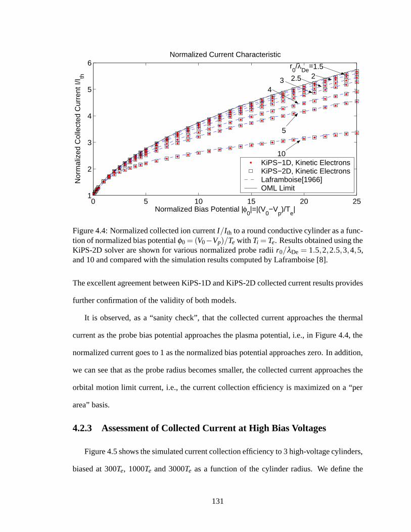
0 5 10 15 20 251
2
3
4
5
6Normalized Current Characteristic
Normalized Bias Potential |φ0|=|(V
0−V
p)/T
e|
Nor
mal
ized
Col
lect
ed C
urre
nt I/
I th
KiPS−1D, Kinetic ElectronsKiPS−2D, Kinetic ElectronsLaframboise[1966]OML Limit
r0/λ
De= 1.5 2 2.5 3
4
5
10
Figure 4.4: Normalized collected ion current I/Ith to a round conductive cylinder as a func-tion of normalized bias potential φ0= (V0−Vp)/Te with Ti= Te. Results obtained using theKiPS-2D solver are shown for various normalized probe radii r0/λDe = 1.5,2,2.5,3,4,5,and 10 and compared with the simulation results computed by Laframboise [8].
The excellent agreement between KiPS-1D and KiPS-2D collected current results provides
further confirmation of the validity of both models.
It is observed, as a “sanity check”, that the collected current approaches the thermal
current as the probe bias potential approaches the plasma potential, i.e., in Figure 4.4, the
normalized current goes to 1 as the normalized bias potential approaches zero. In addition,
we can see that as the probe radius becomes smaller, the collected current approaches the
orbital motion limit current, i.e., the current collection efficiency is maximized on a “per
area” basis.
4.2.3 Assessment of Collected Current at High Bias Voltages
Figure 4.5 shows the simulated current collection efficiency to 3 high-voltage cylinders,
biased at 300Te, 1000Te and 3000Te as a function of the cylinder radius. We define the
131

0 5 10 150.2
0.3
0.4
0.5
0.6
0.7
0.8
0.9
1
Current Ratio I/Ioml
vs Normalized Round Cylinder Radius r0/λ
De (|φ
0|=300)
Normalized Round Cylinder Radius r0/λ
De
I/Iom
l
KiPS−1DKiPS−2D[Estes and SanMartin, 2000]
0 5 10 150.2
0.3
0.4
0.5
0.6
0.7
0.8
0.9
1
Current Ratio I/Ioml
vs Normalized Round Cylinder Radius r0/λ
De (|φ
0|=1000)
Normalized Round Cylinder Radius r0/λ
De
I/Iom
l
KiPS−1D[Estes and SanMartin, 2000]
Figure 4.5: Current ratio I/Ioml (“current collection efficiency”) as a function of the radiusof a round conductive cylinder immersed in a stationary plasma. Results obtained usingthe KiPS-1D and KiPS-2D solvers are shown for two bias potential values of |φ0| = 300and |φ0| = 1000. A comparison is shown with calculations published by Estes and San-martın [12] for Ti = Te.
132

“current collection efficiency” as the ratio of the collected current over the orbital motion
limit current Ioml.
As expected, our results show a decrease in collection efficiency as the cylinder radius
increases, because it results in a gradual breakdown of the orbital motion limit conditions.
As the probe radius becomes larger, an increasing number of attracted-particle orbits con-
nect two points on the probe surface. These unpopulated orbits create voids in the velocity
distribution function of the inbound particles at the probe surface which grow as the probe
radius increases.
Our results are compared against an approximate current calculation performed by
Estes and Sanmartın [12]. The agreement with our simulation results is good, although
not excellent. The source of the discrepancy is most likely the approximations used by
Estes and Sanmartın [12], where an asymptotic approach is used that is only exact in the
limit of thin cylinders. Our kinetic results allow us to confirm that, as observed by Estes
and Sanmartın [12], the collection efficiency appears to be mostly dependent on the cylin-
der radius, and is only a weak function of the bias potential. This behavior provides a fairly
simple rule that could be used by the designer of an electrodynamic tether system in the
determination of an appropriate tether radius.
4.2.4 Plasma Profiles at High Voltages
Having validated our kinetic model in the low voltage regimes for which independent
simulation data are available, we now turn to an important question that was not resolved
by previous work in the field: how does sheath radius generally scale as a function of probe
radius and bias potential?
133

100
101
102
−5000
−4000
−3000
−2000
−1000N
orm
aliz
ed P
oten
tial φ
=| V
/Te |
100
101
102
0
2000
4000
6000
Normalized Radius r / λDe
Cum
ulat
ive
Spa
ce C
harg
e Q
/(ε0 T
e)
Normalized Potential/Space Charge vs Normalized Radius
100
101
102
0
0.2
0.4
0.6
0.8
Normalized Radius r / λDe
Nor
mal
ized
Den
sity
n/n
0
Normalized Densities vs Normalized Radius
Electron DensityIon DensityNet Charge Density
Figure 4.6: Typical high-voltage cylindrical sheath structure shown on a semilog scale.These profiles were obtained using KiPS-1D with a cylinder radius r0 = λDe and a biaspotential φ0 =
V0−VpTe=−5000.
4.2.4.1 Typical Plasma Profile from KiPS-1D
Figure 4.6 shows a typical self-consistent high-voltage plasma profile obtained using
KiPS-1D for a one-Debye-length-radius probe negatively biased at φ0 = −5000 (5000
times the electron temperature). Note that the profiles are shown on a semilog scale to
facilitate their interpretation.
The potential profile shown on the top half of Figure 4.6 is seen to follow a logarithmic
trend out to a radius near 70 Debye lengths, which indicates that space charge effects are
unimportant for smaller radii. To illustrate this, a plot of the “cumulative charge” is shown
on the same figure which confirms that the amount of space charge due to the plasma is
unimportant until we reach a sizable distance from the probe’s surface. The total amount of
134
negative linear surface charge on the cylinder Qn =−6800 (unit-less, normalized value) is
only neutralized by the plasma charge once we reach a radius of about 175 Debye lengths,
at which point the cumulative space charge has reached a value very close to 6800, precisely
balancing out the cylinder surface charge. Much of the charge neutralization thus seems
to occur within an annular region of inner radius rinner = 70λDe and outer radius router =
175λDe.
Because the potential profile has a logarithmic behavior for a sizable portion of the
sheath, a useful approximation for the potential profile can be obtained using linear regres-
sion over its logarithmic portion. This best-fit approximation takes the form
φ = φ0
(1−
ln(r/r0)
ln(rs/r0)
), (4.13)
where r0 is the cylinder radius, and rs is defined as the effective sheath radius. The term
“effective” refers to the fact that the potential profile is effectively the same as that which
would exist if all of the space charge were lumped into a thin cylinder of charge located
at a radius r = rs. This can be thought of as an analogy to a coaxial capacitor, for which
all of the outer charge is located on the outer conductor. Another reason for using the
term “effective sheath radius” instead of simply “sheath radius” is to avoid any confusion
with the classical notion of sheath edge, which is typically defined as the minimum radius
at which the plasma is deemed quasi-neutral based on a somewhat arbitrary definition of
quasi-neutrality [22]. For the present case shown in Figure 4.6, we find for the effective
sheath radius a value of about 100 Debye length, which corresponds to the radius where the
best-fit approximation intercepts a potential of zero. This definition of the sheath radius,
which is based on the specific needs of the charge precipitation application, is believed to
provide a better measure of the effective region of influence of the sheath than the classical
definition and is most appropriate for high voltages, which cause the space charge to lump
within an annular region of limited extent.
135

Now let us consider the density profiles shown on the bottom portion of Figure 4.6.
First, the density of the repelled electrons is, not surprisingly, negligible over the vast ma-
jority of the sheath, having dropped sharply together with the ion density drop. Another ob-
servation of interest is that, as was observed at lower voltages, the ion density here reaches
the orbital motion limit of half of the ambient density (ni/n0 = 0.5), because the cylinder
radius is sufficiently small.
Now, one feature of crucial importance is the very low ion density that exists within
the sheath. The minimum density seen on this particular profile is about 0.05, that is, 5%
of the ambient density. This relatively low value of the minimum ion density is key to
obtaining large sheath sizes because it represents a limitation in the shielding capability of
the ambient plasma.
The very low minimum ion density observed within the sheath extends over a sizable
range at high voltages (keep in mind that the scale used in Figure 4.6 is semi-logarithmic).
This can be interpreted in one of two equivalent ways, which we state here:
Current conservation The quasi-conservation of the radial ion current forces the inward-
directed component of the ion density to drop as the ions accelerate into the potential
well of the sheath. The same reasoning applies equally well to the “outward-directed”
component of the ion density, which must increase as the ions decelerate as they
come out of the potential well. Although simplistic, this explanation can qualitatively
explain the sudden drop of the ion density near a radius r ≈ 150 λDe. The validity
of this reasoning is based on the fact that the vast portion of the incoming ions at the
sheath edge will miss the small probe, so that we may assume that the inward and
outward populations contribute equivalent amounts to the local density. In addition,
most inward ions do not “turn back” before they get in relatively close range from
the cylinder, which allows us to use the argument of conservation of current for the
136

inward and outward populations separately.
Angular Momentum limitations In the region just within the sheath but still far enough
from the cylinder, the ion population is mostly radially-directed because of the ac-
celeration it has experienced as it entered the sheath. In these locations, a large range
of directions with relatively large angular momentum are therefore not populated be-
cause they are located on collisionless “trapped” orbits, i.e., orbits that are closed
onto themselves and do not originate from the background plasma.
The reasons for these reduced ion densities will become more evident as we discuss the
variation of the ion velocity distributions throughout the sheath in Section 4.2.4.4.
4.2.4.2 Typical Two-Dimensional Plasma Structure from KiPS-2D
Figures 4.7 and 4.8 illustrate the 2-D structure of the plasma surrounding the conduc-
tive cylinder, as computed using KiPS-2D, along with corresponding x-axis cross-sectional
profiles. The dynamic meshing capability of KiPS-2D is shown by the high mesh density
near the sheath edge, where a surge in the net charge density is observed. The obtained
profiles are in agreement with results obtained using KiPS-1D.
4.2.4.3 Profile dependence on Bias Potential and Cylinder Radius
It turns out that the value of the minimum ion density goes down as the magnitude of
the bias potential increases, which contributes to a further increase in sheath dimensions.
This is seen in Figures 4.9 and 4.11, which show a set of various density and potential
profiles corresponding to various bias settings for a cylinder of radius r0 = λDe. Similar
families of curves are shown in Figures 4.10 and 4.12 for a much smaller cylinder radius
r0 = 0.001λDe. Although both sets of curves behave somewhat similarly at large radii, the
main difference with the smaller cylinder radius is that the ion density is allowed to ramp
137

−500
50 0
20
40
0
0.1
0.2
0.3
0.4
0.5
0.6
xn=x/λ
De
y n=y
/λ De
ρ in/(
en0)
−50 −30 −10 10 30 50
0.1
0.2
0.3
0.4
0.5
0.6
x/λDe
ρ in/(
e n 0)
(a) Input Net Charge Distribution ρin/(en0)
⇓ (Poisson Solver)⇓
−500
50 0
20
40
−300
−250
−200
−150
−100
−50
xn=x/λ
De
y n=y
/λ De
φ=(V
−V
p)/T
e
−50 −30 −10 10 30 50
−300
−250
−200
−150
−100
−50
x/λDe
φ=(V
−V
p)/T
e
(b) Potential Distribution φ = (V −Vp)/Te
⇓ (Vlasov Solver)⇓
−500
50 0
20
40
0
0.1
0.2
0.3
0.4
0.5
0.6
xn=x/λ
De
y n=y
/λ De
ρ out/(
en0)
−50 −30 −10 10 30 50
0.1
0.2
0.3
0.4
0.5
0.6
x/λDe
ρ out/(
e n 0)
(c) Output Net Charge Distribution ρout/(en0)
Figure 4.7: Poisson–Vlasov consistent solution for the single-cylinder configuration witha cylinder radius r0 = λDe and normalized bias φ0 = −320. Self-consistency is shown bythe similarity of ρin and ρout. 2-D solutions are shown on the left, and corresponding x-axiscross-section profiles are shown on the right. Ion and Electron density dist. are shown inFigure 4.8.
138

−500
50 0
20
40
0.1
0.2
0.3
0.4
0.5
0.6
0.7
0.8
y n=y
/λ De
n e/n0
xn=x/λ
De
−50 −30 −10 10 30 50
0.1
0.2
0.3
0.4
0.5
0.6
0.7
0.8
x/λDe
n e/n0
(a) Normalized Electron Number Density ne/n0.
−500
50 0
20
40
0.2
0.3
0.4
0.5
0.6
0.7
0.8
xn=x/λ
De
y n=y
/λ De
n i/n0
−50 −30 −10 10 30 500.2
0.3
0.4
0.5
0.6
0.7
0.8
x/λDe
n i/n0
(b) Normalized Ion Number Density ni/n0.
Figure 4.8: Poisson–Vlasov consistent electron and ion density distributions correspondingto the single-cylinder solution shown in Figure 4.7 (r0 = λDe, φ0 = −320). These densityprofiles constitute the output of the Vlasov solver and are subtracted to form the output netcharge density profile �ρout = e(ni−ne) shown in Figure 4.7(c).
139

100
101
102
0
0.2
0.4
0.6
0.8
1Normalized Electron Density Profile
Normalized Position r/λDe
Nor
mal
ized
Num
ber
Den
sity
n/n
0
KiPS−1D, Boltzmann ElectronsKiPS−2D, Boltzmann Electrons
φ0=−10
−20 −40
−80 −160
−320 −640 −1280 −2560 −5120
100
101
102
0.2
0.4
0.6
0.8
1Normalized Ion Density Profile
Normalized Position r/λDe
Nor
mal
ized
Num
ber
Den
sity
n/n
0
KiPS−1D, Boltzmann ElectronsKiPS−2D, Boltzmann Electrons
φ0=−10
−40
−80
−160
−320 −640
−1280 −2560 −5120
−20
Figure 4.9: Family of electron and ion density profiles for a round conductive cylinderwith radius r0 = λDe in a stationary plasma. Several curves are shown corresponding tonormalized biases φ0 =V0/Te spanning from −10 to −5120.
140

10−3
10−2
10−1
100
101
102
0
0.2
0.4
0.6
0.8
1Normalized Electron Density Profile
Normalized Position r/λDe
Nor
mal
ized
Num
ber
Den
sity
n/n
0
KiPS−1D, Boltzmann ElectronsKiPS−2D, Boltzmann Electrons
φ0=−10
−20 −40
−80 −160 −320 −640
−1280 −2560 −5120
10−3
10−2
10−1
100
101
102
0.2
0.4
0.6
0.8
1Normalized Ion Density Profile
Normalized Position r/λDe
Nor
mal
ized
Num
ber
Den
sity
n/n
0
KiPS−1D, Boltzmann ElectronsKiPS−2D, Boltzmann Electrons φ
0=−5120 −2560
−1280 −640
−320
−160
−80
−40
Figure 4.10: Family of electron and ion density profiles for a round conductive cylinderwith radius r0 = 0.001λDe in a stationary plasma. Several curves are shown correspondingto normalized biases φ0 =V0/Te spanning from −10 to −5120.
141

100
101
102
−5000
−4000
−3000
−2000
−1000
Normalized Potential Profile
Normalized Position r/λDe
Nor
mal
ized
Pot
entia
l (V
−V
p)/T
e
KiPS−1D, Boltzmann ElectronsKiPS−2D, Boltzmann Electrons
φ0=−5120
−2560
−1280
−640
−320
Figure 4.11: Family of potential profiles for a round conductive cylinder with radius r0 =λDe in a stationary plasma. Several curves are shown corresponding to normalized biasesφ0 =V0/Te spanning from −10 to −5120.
10−3
10−2
10−1
100
101
102
−5000
−4000
−3000
−2000
−1000
Normalized Potential Profile
Normalized Position r/λDe
Nor
mal
ized
Pot
entia
l (V
−V
p)/T
e
KiPS−1D, Boltzmann ElectronsKiPS−2D, Boltzmann Electrons
φ0=−5120
−2560
−1280
−640 −320
Figure 4.12: Family of potential profiles for a round conductive cylinder with radius r0 =0.001λDe in a stationary plasma. Several curves are shown corresponding to normalizedbiases φ0 =V0/Te spanning from −10 to −5120.
142

back up to the ambient density due to an improved geometric convergence at smaller radii,
before dropping back to half of the ambient density at the probe surface, the orbital motion
limit.
4.2.4.4 Variation of the Ion Velocity Distribution Throughout the Sheath
In order to better understand the nature of the pronounced ion density drop in the sheath,
we now inspect the ion velocity distribution functions throughout the sheath. Since within
the potential well, the velocity distributions are getting compressed onto a thin annulus, a
perhaps better graphical representation of the velocity distribution function can be obtained
using the concept of directional-energy distribution, which we now define. Let E be the
total particle energy, including both potential and kinetic energy components. At a given
location in the plasma, we may write E as
E = qiV +mi
2
(v2
r + v2θ)
(4.14)
where V is the local potential, qi = e is the ion charge, mi is the ion mass, and the instanta-
neous velocity components in cylindrical coordinates are vr and vθ . In the ambient plasma
(as r→ ∞), the total energy distribution of the ions is a Maxwellian:
fE(E) =n0
eTexp
(−
ET
). (4.15)
As we get closer to the sheath, the total energy distribution is no longer isotropic, so we
introduce the concept of “directional-energy” f (Er,Eθ ), where Er and Eθ are defined as
Er = Evr√
v2r + v2
θ
, and Eθ = Evθ√
v2r + v2
θ
. (4.16)
The directional distribution of particles can thus be given as a function of the two variables
Er and Eθ .
Figure 4.13 depicts the directional-energy distributions at various locations along the
ion density profile.
143

Figure 4.13: Ion “directional-energy” distributions in the high-voltage cylindrical sheath.
144

In the following we describe the nature of the velocity distributions as applicable to
the various distributions labeled from 1 to 22 in Figure 4.13, going from the largest radius
(point 1, farthest location) to the probe surface (point 22):
Locations No. 1–2 The inbound ions are Maxwellian. The outbound ions are only par-
tially blocked out by the probe (probe shadow effect).
Location No. 3 The probe shadow grows as we get closer to the probe, just outside the
sheath. Some very small unpopulated trapped orbits start to appear, due to some
angular momentum limitations.
Location No. 4 The probe shadow is unchanged. The zone of unpopulated trapped orbits
is rapidly expanding as we enter the sheath and ions are radially accelerated.
Location No. 5 The probe shadow now starts shrinking as we enter the sheath, since the
“shadowed trajectories” are also being radially accelerated. The zone of unpopulated
trapped orbits continues to expand significantly, and the directional-energy distribu-
tion appears to be increasingly radially-directed.
Locations No. 6–13 The probe shadow is fairly small within the sheath since shadowed
trajectories are very radially directed. The ions are almost exclusively radially di-
rected. The ion density has dropped significantly because of the radial acceleration
as we enter the sheath, leaving the inaccessible large-angular-momentum orbits un-
populated. The ion density reaches its minimum at location No.7. Beyond this point,
geometrical concentration of current will overcome the sheath acceleration effects
and gradually populate the depleted zones, causing the density to increase.
Locations No. 14–20 The probe shadow is now growing as we near the probe. Geomet-
rical concentration of current has overcome the sheath acceleration effects and the
145

depleted zones are gradually getting filled as we near the probe.
Location No. 21 There are virtually no unpopulated trapped zones anymore. This is be-
cause we have reached a small enough radius for geometrical concentration to have
re-populated the depleted zones.
Location No. 22 We are now at the surface of this one-Debye-length-radius probe. Half
of the directions are blocked by the probe, and consequently the density is half the
ambient density. There are no unpopulated incoming directions at the surface of this
small probe, which is why the surface ion density achieves its maximum possible
value of half the ambient density; this is the orbital motion limit. A larger probe
would result in a lower ion density because it would feature depleted zones which
would correspond to a set of orbits linking two points on the probe’s surface.
4.2.5 Sheath Radius at High Voltages
Having defined an effective sheath radius rs consistent with an asymptotic best-fit of
the potential profile given by (4.13), we now consider the effect of the bias potential φ0
and probe radius r0 on the effective sheath radius rs. The top part of Figure 4.14 shows
the variation of the normalized effective sheath radius rs as a function of the normalized
bias potential φ0, for several values of the cylinder radius r0. Not surprisingly, the effective
sheath radius grows for increasing bias potential magnitudes and also grows monotonically
as a function of the cylinder radius r0.
As we have discussed before, at large voltages the space charge in the immediate vicin-
ity of the probe should have a negligible effect on the local potential which is overwhelm-
ingly dominated by the effect of the cylinder surface charge. For sufficiently thin cylinders,
which cause little shadowing effect on outbound trajectories over most of the sheath, the
electrodynamic processes in the bulk of the sheath should become nearly independent of
146
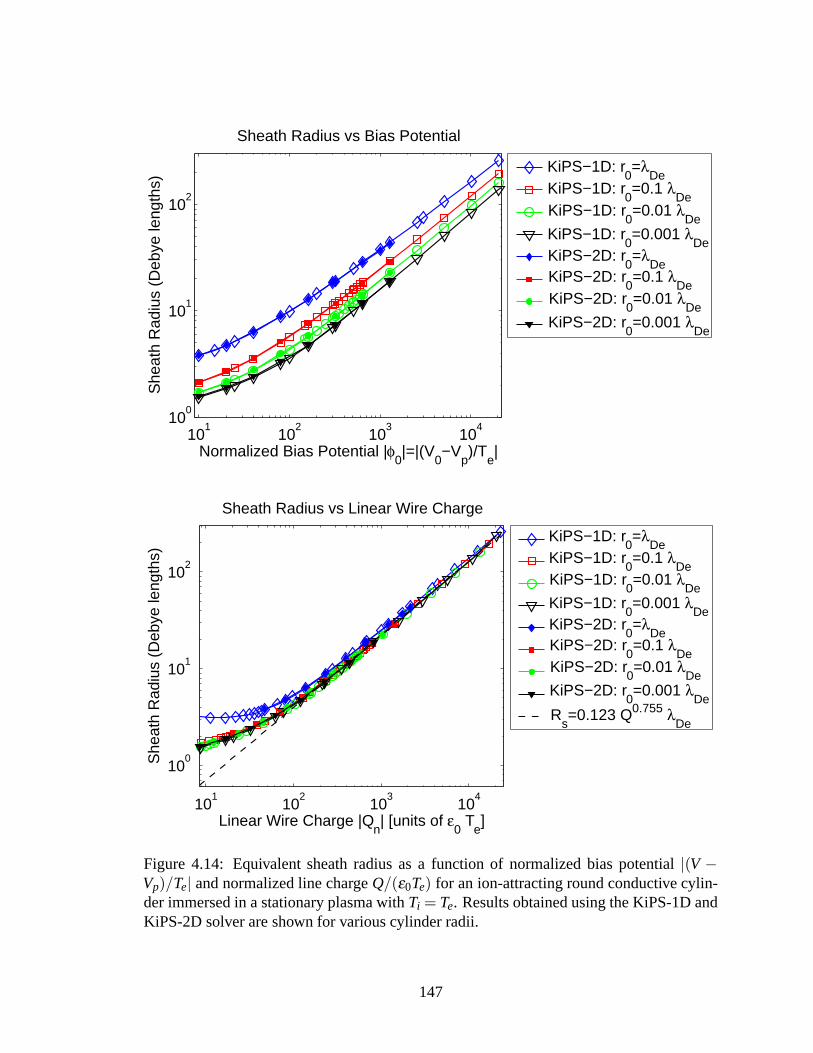
101
102
103
104
100
101
102
Normalized Bias Potential |φ0|=|(V
0−V
p)/T
e|
She
ath
Rad
ius
(Deb
ye le
ngth
s)Sheath Radius vs Bias Potential
KiPS−1D: r0=λ
De
KiPS−1D: r0=0.1 λ
De
KiPS−1D: r0=0.01 λ
De
KiPS−1D: r0=0.001 λ
De
KiPS−2D: r0=λ
De
KiPS−2D: r0=0.1 λ
De
KiPS−2D: r0=0.01 λ
De
KiPS−2D: r0=0.001 λ
De
101
102
103
104
100
101
102
Linear Wire Charge |Qn| [units of ε
0 T
e]
She
ath
Rad
ius
(Deb
ye le
ngth
s)
Sheath Radius vs Linear Wire Charge
KiPS−1D: r0=λ
De
KiPS−1D: r0=0.1 λ
De
KiPS−1D: r0=0.01 λ
De
KiPS−1D: r0=0.001 λ
De
KiPS−2D: r0=λ
De
KiPS−2D: r0=0.1 λ
De
KiPS−2D: r0=0.01 λ
De
KiPS−2D: r0=0.001 λ
De
Rs=0.123 Q0.755 λ
De
Figure 4.14: Equivalent sheath radius as a function of normalized bias potential |(V −Vp)/Te| and normalized line charge Q/(ε0Te) for an ion-attracting round conductive cylin-der immersed in a stationary plasma with Ti = Te. Results obtained using the KiPS-1D andKiPS-2D solver are shown for various cylinder radii.
147

the cylinder radius for a given cylinder surface charge. Instead of plotting the sheath radius
as a function of bias potential, on the bottom part of Figure 4.14 we now plot it against
the magnitude of the negative linear charge present on the cylinder’s surface, which can be
obtained through one of two equivalent methods:
• by integrating the positive total plasma space charge surrounding the cylinder, which
is equal and opposite to the total negative charge held by the cylinder;
• by inferring it from the knowledge of the cylinder radius r0, bias φ0 and effective
sheath radius rs using the linear capacitance formula for a coaxial capacitor [43],
Qn =2πφ0
ln rsr0
. (4.17)
All of the plots shown on the top part of Figure 4.14 now align over each other on the bot-
tom part, except for the plot corresponding to the largest tested cylinder radius of r0 = λDe.
This remaining discrepancy is due to the fact that this cylinder radius is sufficiently large
to cause significant shadowing of some outbound ion trajectories which are left unpopu-
lated, causing a reduction of the ion density throughout the sheath and a reduced shielding
capability consistent with the observed larger sheath size as compared to cases with equal
surface charge but smaller cylinder radius r0.
As is shown on the bottom part of Figure 4.14, an asymptotic best-fit of the rs-vs-Qn
relationship was performed over the highest values of the linear wire charge Qn, which
applies accurately for |Qn| ≥ 200 and r0 ≤ 0.1λDe. This best-fit asymptotic relationship is
given by
rs
λDe= 0.123 |Qn|
0.755 . (4.18)
Although this equation is not accurate for larger cylinder radii as is seen for r0 = λDe
on the bottom part of Figure 4.14, it may still be used for purposes of determining a lower
148

bound. This asymptotic equation can now be combined with (4.17) to determine an implicit
asymptotic equation for the effective sheath radius rs as a function of the bias potential φ0:
2.554
(rs
λDe
)1.325
lnrs
r0=−φ0. (4.19)
Although this equation cannot be solved analytically for rs, it can be inverted numerically
or computed directly for a given set of negative values for the bias potential φ0. Consistent
with the restrictions mentioned above, it can be used to accurately predict sheath radii for
cylinder radii of a tenth of a Debye length or less (r0 <= 0.1λDe) and for bias potentials φ0
with a magnitude such that
|φ0| ≥2002π
lnrs
r0≈ 31.8ln
rs
r0. (4.20)
For values of the bias potential φ0 and cylinder radius r0 beyond these limits, the sheath
dimensions given by numerically solving (4.19) should be regarded as lower bounds.
4.3 Interference of Parallel Round Cylinders in a Station-ary Plasma
In an effort to gain a basic understanding of the physics of plasma-immersed multi-
wire conductive structures, we consider a structure consisting of two parallel, identical
round cylinders with equal bias potential (see Figure 1.3(b)). The geometrical parameters
are the cylinder radius r0 and the center-to-center spacing ∆x. All of the simulation results
presented in this section were performed using a cylinder radius r0 = λDe and a normalized
bias potential φ0 =V0−Vp
Te=−320.
We consider the effect of the center-to-center spacing on sheath structure and current
collection, always comparing performances to those of a single round cylinder with radius
r0 = λDe and bias potential φ0 = −320. The value of the center-to-center spacing ∆x will
vary from ∆x = λDe (cylinders touching) all the way to ∆x = 200λDe. This maximum
149
spacing corresponds to about 10.5 times the single-wire effective sheath radius of 19λDe
(see Figure 4.14).
In the negative bias potential situation under consideration, the ions are the attracted
species. Since the plasma is not moving (no flow), the results we obtain are also directly
applicable to the electron-attracting situation with equal and opposite bias potential, pro-
vided that we swap the ion and electron density profiles.
4.3.1 Treatment of Repelled Electrons
Our model allows for the full kinetic representation of both species. However, in a
stationary situation we know that the electric potential will have the same sign as the bias
potential, everywhere in space around the perturbation, and certainly everywhere within
the computational zone. For a repelling bias potential of such a large magnitude as that
considered here (φ0 = −320), we can affirm that, for all practical purposes, none of the
electron trajectories which contribute to the electron density intersect the conductive cylin-
ders. This means that all electron trajectories are connected to the background plasma, and
allows us to use with excellent accuracy the Boltzmann equation for the electron density:
ne = n0 expVTe, (4.21)
where we assume that V < 0 everywhere in space, and arbitrarily set the plasma potential
to zero. This approach results in significant computational savings, due to the fact that only
the ions need to be treated kinetically.
4.3.2 Orbits of the Attracted Ions
We now turn our attention to the orbits of the attracted ions. In the following we discuss
the existence of complex ion orbits which do not exist in the single-cylinder case, and
explain that the criteria used to determine whether an orbit is trapped (and unpopulated)
150

must be less restrictive than in the case of the single cylinder. We then show some examples
of these complex orbits.
4.3.2.1 Criteria for Trapped Orbits
The symmetric potential structure which exists in the simple single-cylinder case does
not allow any of the non-trapped trajectories to feature more than one change of “radial
direction”, that is, one change of sign of the radial component of velocity, vr. In other
words, any orbit originating from the background plasma will either:
• approach the conductive cylinder (vr < 0), miss it due to an excessive angular mo-
mentum and return to the background plasma (vr > 0);
• approach the conductive cylinder and get collected onto it (vr < 0 all along).
When two parallel cylinders immersed in a plasma are placed sufficiently close to one
another (i.e., when the individual sheath radius is a non-negligible fraction of the center-to-
center spacing ∆x), the shadow effect created by one cylinder can affect the space charge
surrounding the other sufficiently to create asymmetries in the potential structure. Those
asymmetries, in turn, could allow for the existence of collisionless trajectories of an in-
creased complexity, featuring for example several “radial oscillations” about a given cylin-
der, or even “figure eight” trajectories orbiting about both cylinders. At any given location,
some of the directions in velocity space that were unpopulated when there was no neigh-
boring cylinder may now be populated through relatively complex paths originating from
the background plasma, while other directions that were previously populated may now be
unpopulated due to the existence of new types of trapped orbits, such as the “figure eight”.
As a consequence, the simulation parameters used to determine whether a trajectory is
trapped or not will be especially important for this asymmetric structure. We need to set a
sufficiently large radial oscillation limit to allow for the existence of these more complex
151

orbits (described in Section 2.4.2.2), while at the same time keeping it down to a reason-
able value to obtain reasonable simulation times. We have found that allowing for up to
20 radial oscillations (Mrosc = 20) provided such a compromise. The maximum angular
displacement Morb (see Section 2.4.2.2) was not used to impose further restrictions on the
orbits, and Msegcross was set to 100.
4.3.2.2 Examples of Ion Orbits
In Figure 4.15 we show a few typical examples of ion orbits across the self-consistent
potential structure of the two-cylinder configuration with a center-to-center spacing ∆x =
20λDe, a bias potential φ0=−320Te and a cylinder radius r0= λDe. The circle shown at one
end of each trajectory indicates the location of the interrogation point where the velocity
distribution function is being sampled. Following the trajectory from this point backward
in time leads us to the “source” point of the trajectory, indicated by a square.
The source point can be either the background plasma, a cylinder’s surface (in which
case the orbit is unpopulated since the cylinder is not a source), or it may be undetermined
in the case of a trapped orbit.
Figures 4.15(a)–4.15(c) have a common interrogation point, located on a node on the
right side of the mesh. Figure 4.15(a) shows an example of an unpopulated orbit originating
from the surface of the rightmost cylinder; this orbit is not populated because the cylinder
is not a plasma source. Figure 4.15(b) depicts a populated orbit that undergoes two loops
around the rightmost cylinder before reaching the interrogation point, on the outer edge of
the computational zone. Figure 4.15(c) depicts a very complex but populated ion orbit that
originates from the background plasma, undergoes several loops around both cylinders, and
finally reaches the interrogation point.
Figure 4.15(d) corresponds to a different interrogation point. It is shown here to illus-
trate one example of an unpopulated orbit that was deemed “trapped”, having exceeded the
152

−50 0 50
−60
−40
−20
0
20
40
60
Ion Energy = 0.75 Te
x/λDe
y/λ D
e
(a) Unpopulated Orbit Originating FromCylinder Surface
−50 0 50
−60
−40
−20
0
20
40
60
Ion Energy = 1.95 Te
x/λDe
y/λ D
e(b) Complex Populated Orbit Around OneCylinder
−50 0 50
−60
−40
−20
0
20
40
60
Ion Energy = 2.25 Te
x/λDe
y/λ D
e
(c) Complex Populated Orbit Around BothCylinders
−50 0 50
−60
−40
−20
0
20
40
60
Ion Energy = 1 Te
x/λDe
y/λ D
e
(d) Complex Unpopulated Orbit AroundBoth Cylinders
Figure 4.15: Examples of some typical ion orbits within the self-consistent potential struc-ture of a two-cylinder system. The square and circle indicate the source and interrogationpoints of the orbits, respectively. The total ion energy (potential plus kinetic) is indicatedabove each plot in terms of the electron temperature (in units of eV). Intersections with thebackground mesh are marked with small dots.
153

maximum number of radial oscillations set for this simulation, which was Mrosc = 20.
4.3.3 Inspection of the 2-D Sheath Structure
We now consider the general aspect of the sheath structure surrounding both cylinders
for a few values of the center-to-center spacing: ∆x = 2λDe,10λDe,20λDe,40λDe,80λDe,
and 160λDe. First, we note that all of the two-cylinder simulations presented here were
performed using two axes of symmetry, as described in Section 2.6.2.2. In other words,
only a single quadrant had to be simulated, thanks to the symmetry of the two-cylinder
geometry and the fact that the plasma is not flowing. The distributions are shown over two
quadrants, in order to clearly illustrate the two-cylinder geometry under consideration. The
simulation results, performed in the quadrant θ ∈ [0,π/2], were simply “mirrored” to the
second quadrant in θ ∈ [π/2,π]. We have opted to only show the results in the half-space
θ ∈ [0,π], so that the features of interest near the cylinders can be clearly seen. All of the
distributions shown in Figures 4.16 through 4.25 are given in the following two formats:
• 2-D distributions are shown on the left, over the half-space θ ∈ [0,π];
• profiles of cross-sections performed along the x axis are shown on the right.
The self-consistency of the solutions that we show here can be verified by comparing the
distributions for �ρin and �ρout, which correspond to the input and output of the Poisson–
Vlasov operator as specified in Figure 2.3. The distributions for �ρin and �ρout shown in
Figures 4.16, 4.18, 4.20, 4.22, 4.24, and 4.26, are very close to one another, which proves
the self-consistent nature of the solutions.
Figures 4.16 and 4.17 show the distributions pertaining to the smallest center-to-center
spacing, ∆x = 2λDe (cylinders touching). Due to the proximity of the two cylinders, the
profiles obtained are very close to what would be obtained with a single cylinder. The
ion density, shown in Figure 4.17(b), is seen to drop to half the ambient density on the
154
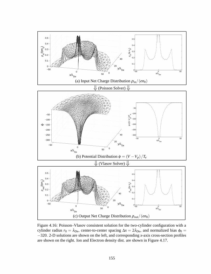
−500
50 0
20
40
0
0.1
0.2
0.3
0.4
0.5
ρ in/(
en0)
x/λDe
y/λDe
−50 0 50
0
0.1
0.2
0.3
0.4
0.5
x/λDe
ρ in/(
e n 0)
(a) Input Net Charge Distribution ρin/(en0)
⇓ (Poisson Solver)⇓
−500
50 0
20
40
−300
−250
−200
−150
−100
−50
φ
x/λDe
y/λDe
−50 0 50
−300
−250
−200
−150
−100
−50
x/λDe
φ=(V
−V
p)/T
e
(b) Potential Distribution φ = (V −Vp)/Te
⇓ (Vlasov Solver)⇓
−500
50 0
20
40
0
0.1
0.2
0.3
0.4
0.5
y/λDe
x/λDe
ρ out/(
en0)
−50 0 500
0.1
0.2
0.3
0.4
0.5
x/λDe
ρ out/(
e n 0)
(c) Output Net Charge Distribution ρout/(en0)
Figure 4.16: Poisson–Vlasov consistent solution for the two-cylinder configuration with acylinder radius r0 = λDe, center-to-center spacing ∆x = 2λDe, and normalized bias φ0 =−320. 2-D solutions are shown on the left, and corresponding x-axis cross-section profilesare shown on the right. Ion and Electron density dist. are shown in Figure 4.17.
155

−500
50 0
20
400.1
0.2
0.3
0.4
0.5
0.6
0.7
ne/n
0
x/λDe
y/λDe
−50 0 50
0.1
0.2
0.3
0.4
0.5
0.6
0.7
x/λDe
n e/n0
(a) Normalized Electron Number Density ne/n0.
−500
50 0
20
40
0.1
0.2
0.3
0.4
0.5
0.6
0.7
ni/n
0
x/λDe
y/λDe
−50 0 50
0.1
0.2
0.3
0.4
0.5
0.6
0.7
x/λDe
n i/n0
(b) Normalized Ion Number Density ni/n0.
Figure 4.17: Poisson–Vlasov consistent electron and ion density distributions correspond-ing to the solution shown in Figure 4.16 (r0 = λDe, φ0 =−320, ∆x= 2λDe). These densityprofiles constitute the output of the Vlasov solver and are subtracted to form the output netcharge density profile �ρout = e(ni−ne) shown in Figure 4.16(c).
156
external surfaces of both cylinders, as is expected. Angular momentum limitations/ion
radial acceleration are responsible for the significant drop in density as the ions enter the
sheath, similar to what was seen in the single-cylinder case.
Figures 4.18 and 4.19 pertain to the spacing ∆x= 10λDe. The potential is seen to drop
in magnitude in between the two cylinders, to a potential φ ≈ −235 from a bias potential
of φ0 =−320. A similar drop of the ion density is seen in Figure 4.19(b) as the ions enter
the sheath, with a minimum density of about 0.2n0. A relatively large ion density is seen
to exist in between the two cylinders, which reaches a maximum of about 0.7n0 but only
has limited extent. The ion density at the surfaces of the cylinders is seen to be much lower
here than what was seen for the case where the cylinders are touching. The ion densities on
the external and internal surfaces of the cylinders are about 0.27n0 and 0.19n0, respectively.
This is an indication that the orbital-motion-limit was not achieved for current collection,
due to the overall extent of this “two-cylinder” probe. The center-to-center spacing is not
quite large enough for the two sheaths to have separated, so that the two cylinders are in
effect emulating a larger structure, leading to reduced current collection, similar to what
was seen for large cylinder radii in Figure 4.5.
Figures 4.20 and 4.21 pertain to the spacing ∆x = 20λDe. Here the potential is seen to
drop down in magnitude to φ ≈−150 in between the two cylinders; the electric fields from
both cylinders are still strongly coupling. The ion density profile presents various “bumps”
as we enter the sheath, which may be due to the partial filling of some of the velocity space’s
directions that were left empty in the single-cylinder case due to angular momentum restric-
tions. Some of these directions are being populated by the complex trajectories described in
Section 4.3.2. Those “bumps” may also be attributed, in part, to some momentum inaccura-
cies on some of the convoluted ion trajectories, due to the piecewise-linear approximation
used for the potential structure. The ion acceleration through the sheath still results in a
157
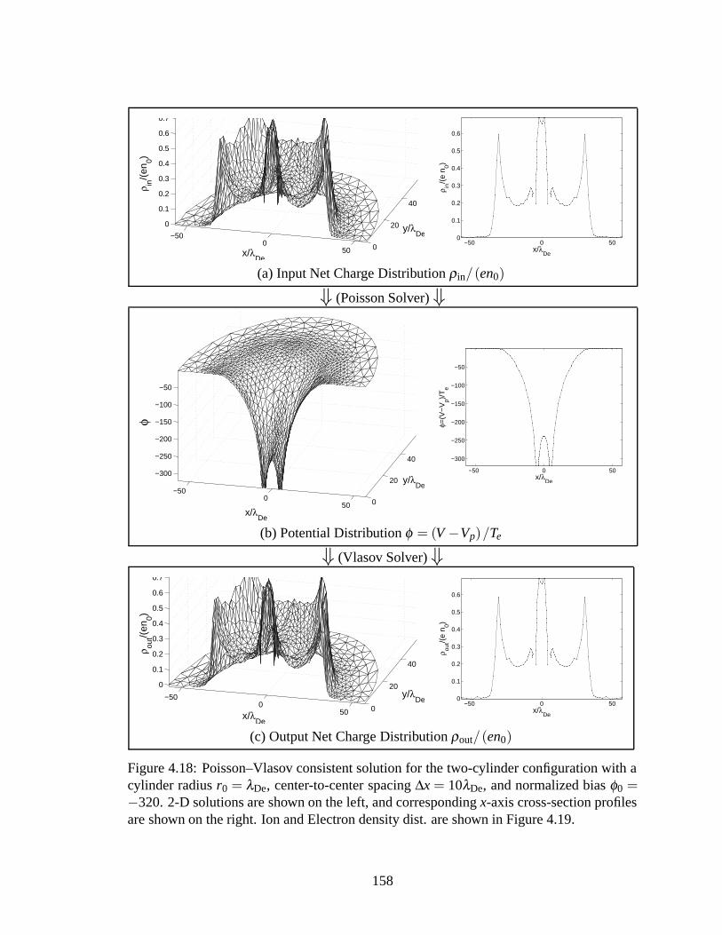
−500
50 0
20
40
0
0.1
0.2
0.3
0.4
0.5
0.6
0.7
ρ in/(
en0)
x/λDe
y/λDe
−50 0 50
0
0.1
0.2
0.3
0.4
0.5
0.6
x/λDe
ρ in/(
e n 0)
(a) Input Net Charge Distribution ρin/(en0)
⇓ (Poisson Solver)⇓
−500
50 0
20
40
−300
−250
−200
−150
−100
−50
φ
x/λDe
y/λDe
−50 0 50
−300
−250
−200
−150
−100
−50
x/λDe
φ=(V
−V
p)/T
e
(b) Potential Distribution φ = (V −Vp)/Te
⇓ (Vlasov Solver)⇓
−500
50 0
20
40
0
0.1
0.2
0.3
0.4
0.5
0.6
0.7
ρ out/(
en0)
x/λDe
y/λDe
−50 0 50
0
0.1
0.2
0.3
0.4
0.5
0.6
x/λDe
ρ out/(
e n 0)
(c) Output Net Charge Distribution ρout/(en0)
Figure 4.18: Poisson–Vlasov consistent solution for the two-cylinder configuration with acylinder radius r0 = λDe, center-to-center spacing ∆x = 10λDe, and normalized bias φ0 =−320. 2-D solutions are shown on the left, and corresponding x-axis cross-section profilesare shown on the right. Ion and Electron density dist. are shown in Figure 4.19.
158

−500
50 0
20
400.1
0.2
0.3
0.4
0.5
0.6
0.7
0.8
ne/n
0
x/λDe
y/λDe
−50 0 50
0.1
0.2
0.3
0.4
0.5
0.6
0.7
0.8
x/λDe
n e/n0
(a) Normalized Electron Number Density ne/n0.
−500
50 0
20
40
0.2
0.3
0.4
0.5
0.6
0.7
0.8
ni/n
0
x/λDe
y/λDe
−50 0 500.2
0.3
0.4
0.5
0.6
0.7
0.8
x/λDe
n i/n0
(b) Normalized Ion Number Density ni/n0.
Figure 4.19: Poisson–Vlasov consistent electron and ion density distributions correspond-ing to the solution shown in Figure 4.18 (r0= λDe, φ0 =−320, ∆x= 10λDe). These densityprofiles constitute the output of the Vlasov solver and are subtracted to form the output netcharge density profile �ρout = e(ni−ne) shown in Figure 4.18(c).
159

−60 −40 −20 0 20 40 60 0
20
40
60
0
0.1
0.2
0.3
0.4
0.5
0.6
ρ in/(
en0)
x/λDe
y/λDe
−60 −40 −20 0 20 40 600
0.1
0.2
0.3
0.4
0.5
x/λDe
ρ in/(
e n 0)
(a) Input Net Charge Distribution ρin/(en0)
⇓ (Poisson Solver)⇓
−60 −40 −20 0 20 40 60 0
20
40
60
−300
−250
−200
−150
−100
−50
φ
y/λDe
x/λDe
−60 −40 −20 0 20 40 60
−300
−250
−200
−150
−100
−50
x/λDe
φ=(V
−V
p)/T
e
(b) Potential Distribution φ = (V −Vp)/Te
⇓ (Vlasov Solver)⇓
−60 −40 −20 0 20 40 60 0
20
40
60
0
0.1
0.2
0.3
0.4
0.5
0.6
y/λDe
x/λDe
ρ out/(
en0)
−60 −40 −20 0 20 40 600
0.1
0.2
0.3
0.4
0.5
x/λDe
ρ out/(
e n 0)
(c) Output Net Charge Distribution ρout/(en0)
Figure 4.20: Poisson–Vlasov consistent solution for the two-cylinder configuration with acylinder radius r0 = λDe, center-to-center spacing ∆x = 20λDe, and normalized bias φ0 =−320. 2-D solutions are shown on the left, and corresponding x-axis cross-section profilesare shown on the right. Ion and Electron density dist. are shown in Figure 4.21.
160

−60 −40 −20 0 20 40 60 0
20
40
60
0.1
0.2
0.3
0.4
0.5
0.6
0.7
0.8
ne/n
0
x/λDe
y/λDe
−60 −40 −20 0 20 40 60
0.1
0.2
0.3
0.4
0.5
0.6
0.7
0.8
x/λDe
n e/n0
(a) Normalized Electron Number Density ne/n0.
−60 −40 −20 0 20 40 60 0
20
40
60
0.2
0.3
0.4
0.5
0.6
0.7
0.8
ni/n
0
x/λDe
y/λDe
−60 −40 −20 0 20 40 600.2
0.3
0.4
0.5
0.6
0.7
0.8
x/λDe
n i/n0
(b) Normalized Ion Number Density ni/n0.
Figure 4.21: Poisson–Vlasov consistent electron and ion density distributions correspond-ing to the solution shown in Figure 4.20 (r0= λDe, φ0 =−320, ∆x= 20λDe). These densityprofiles constitute the output of the Vlasov solver and are subtracted to form the output netcharge density profile �ρout = e(ni−ne) shown in Figure 4.20(c).
161
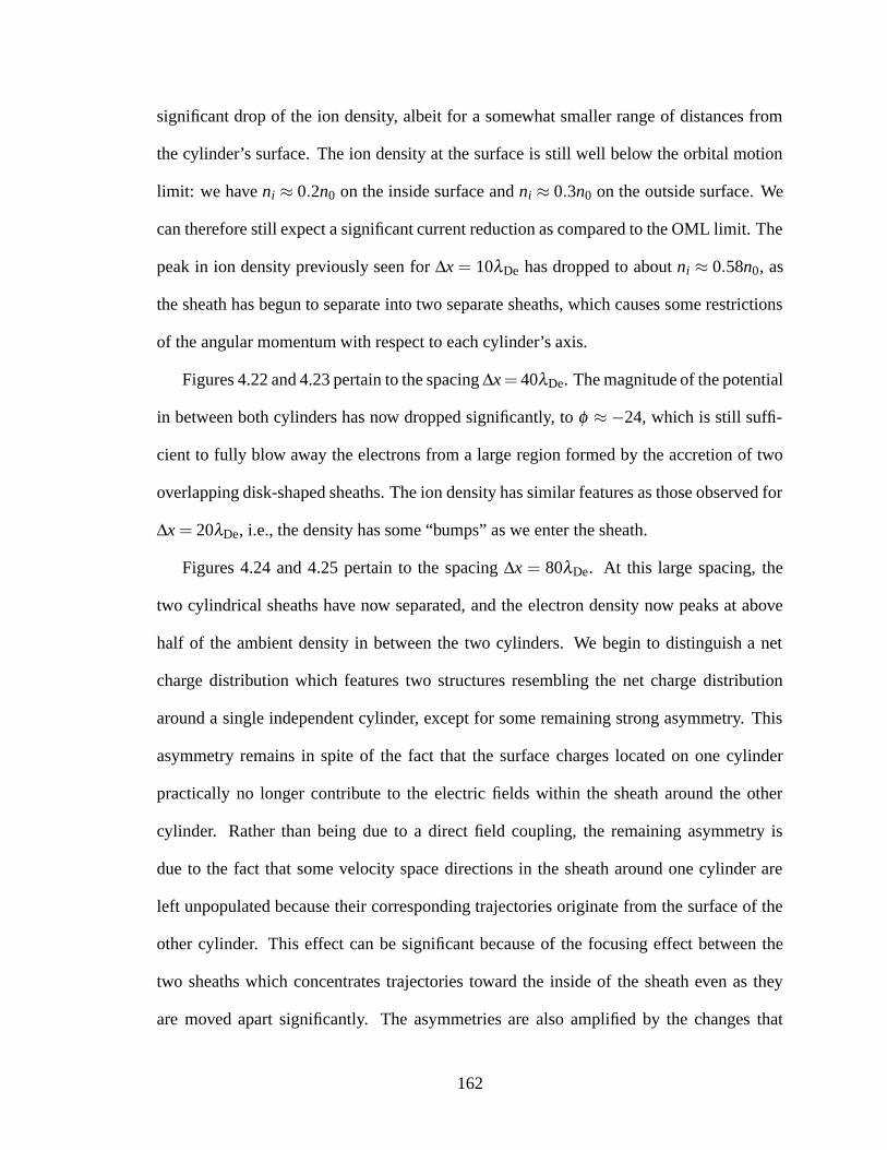
significant drop of the ion density, albeit for a somewhat smaller range of distances from
the cylinder’s surface. The ion density at the surface is still well below the orbital motion
limit: we have ni ≈ 0.2n0 on the inside surface and ni ≈ 0.3n0 on the outside surface. We
can therefore still expect a significant current reduction as compared to the OML limit. The
peak in ion density previously seen for ∆x = 10λDe has dropped to about ni ≈ 0.58n0, as
the sheath has begun to separate into two separate sheaths, which causes some restrictions
of the angular momentum with respect to each cylinder’s axis.
Figures 4.22 and 4.23 pertain to the spacing ∆x= 40λDe. The magnitude of the potential
in between both cylinders has now dropped significantly, to φ ≈ −24, which is still suffi-
cient to fully blow away the electrons from a large region formed by the accretion of two
overlapping disk-shaped sheaths. The ion density has similar features as those observed for
∆x= 20λDe, i.e., the density has some “bumps” as we enter the sheath.
Figures 4.24 and 4.25 pertain to the spacing ∆x = 80λDe. At this large spacing, the
two cylindrical sheaths have now separated, and the electron density now peaks at above
half of the ambient density in between the two cylinders. We begin to distinguish a net
charge distribution which features two structures resembling the net charge distribution
around a single independent cylinder, except for some remaining strong asymmetry. This
asymmetry remains in spite of the fact that the surface charges located on one cylinder
practically no longer contribute to the electric fields within the sheath around the other
cylinder. Rather than being due to a direct field coupling, the remaining asymmetry is
due to the fact that some velocity space directions in the sheath around one cylinder are
left unpopulated because their corresponding trajectories originate from the surface of the
other cylinder. This effect can be significant because of the focusing effect between the
two sheaths which concentrates trajectories toward the inside of the sheath even as they
are moved apart significantly. The asymmetries are also amplified by the changes that
162
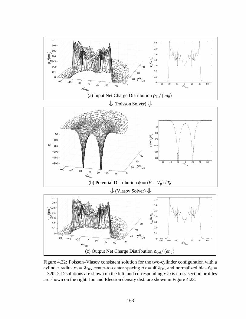
−60 −40 −20 0 20 40 60 0
20
40
60
0
0.1
0.2
0.3
0.4
0.5
0.6
0.7
ρ in/(
en0)
x/λDe
y/λDe
−60 −40 −20 0 20 40 60
0
0.1
0.2
0.3
0.4
0.5
0.6
0.7
x/λDe
ρ in/(
e n 0)
(a) Input Net Charge Distribution ρin/(en0)
⇓ (Poisson Solver)⇓
−60 −40 −20 0 20 40 60 0
20
40
60
−300
−250
−200
−150
−100
−50
φ
x/λDe
y/λDe
−60 −40 −20 0 20 40 60
−300
−250
−200
−150
−100
−50
x/λDe
φ=(V
−V
p)/T
e
(b) Potential Distribution φ = (V −Vp)/Te
⇓ (Vlasov Solver)⇓
−60 −40 −20 0 20 40 60 0
20
40
60
0
0.1
0.2
0.3
0.4
0.5
0.6
0.7
ρ out/(
en0)
x/λDe
y/λDe
−60 −40 −20 0 20 40 60
0
0.1
0.2
0.3
0.4
0.5
0.6
0.7
x/λDe
ρ out/(
e n 0)
(c) Output Net Charge Distribution ρout/(en0)
Figure 4.22: Poisson–Vlasov consistent solution for the two-cylinder configuration with acylinder radius r0 = λDe, center-to-center spacing ∆x = 40λDe, and normalized bias φ0 =−320. 2-D solutions are shown on the left, and corresponding x-axis cross-section profilesare shown on the right. Ion and Electron density dist. are shown in Figure 4.23.
163

−60 −40 −20 0 20 40 60 0
20
40
60
0.1
0.2
0.3
0.4
0.5
0.6
0.7
0.8
ne/n
0
x/λDe
y/λDe
−60 −40 −20 0 20 40 60
0.1
0.2
0.3
0.4
0.5
0.6
0.7
0.8
x/λDe
n e/n0
(a) Normalized Electron Number Density ne/n0.
−60 −40 −20 0 20 40 60 0
20
40
60
0.3
0.4
0.5
0.6
0.7
0.8
ni/n
0
x/λDe
y/λDe
−60 −40 −20 0 20 40 600.3
0.4
0.5
0.6
0.7
0.8
x/λDe
n i/n0
(b) Normalized Ion Number Density ni/n0.
Figure 4.23: Poisson–Vlasov consistent electron and ion density distributions correspond-ing to the solution shown in Figure 4.22 (r0= λDe, φ0 =−320, ∆x= 40λDe). These densityprofiles constitute the output of the Vlasov solver and are subtracted to form the output netcharge density profile �ρout = e(ni−ne) shown in Figure 4.22(c).
164

−500
50 0
20
40
60
80
0
0.1
0.2
0.3
0.4
0.5
0.6
0.7
y/λDe
x/λDe
ρ in/(
en0)
−50 0 500
0.1
0.2
0.3
0.4
0.5
0.6
0.7
x/λDe
ρ in/(
e n 0)
(a) Input Net Charge Distribution ρin/(en0)
⇓ (Poisson Solver)⇓
−500
50 0
20
40
60
80
−300
−250
−200
−150
−100
−50
φ
x/λDe
y/λDe
−50 0 50
−300
−250
−200
−150
−100
−50
x/λDe
φ=(V
−V
p)/T
e
(b) Potential Distribution φ = (V −Vp)/Te
⇓ (Vlasov Solver)⇓
−500
50 0
20
40
60
80
0
0.1
0.2
0.3
0.4
0.5
0.6
0.7
ρ out/(
en0)
x/λDe
y/λDe
−50 0 50
0
0.1
0.2
0.3
0.4
0.5
0.6
0.7
x/λDe
ρ out/(
e n 0)
(c) Output Net Charge Distribution ρout/(en0)
Figure 4.24: Poisson–Vlasov consistent solution for the two-cylinder configuration with acylinder radius r0 = λDe, center-to-center spacing ∆x = 80λDe, and normalized bias φ0 =−320. 2-D solutions are shown on the left, and corresponding x-axis cross-section profilesare shown on the right. Ion and Electron density dist. are shown in Figure 4.25.
165
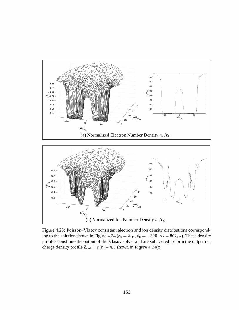
−500
50 0
20
40
60
80
0.1
0.2
0.3
0.4
0.5
0.6
0.7
0.8
ne/n
0
x/λDe
y/λDe
−50 0 50
0.1
0.2
0.3
0.4
0.5
0.6
0.7
0.8
x/λDe
n e/n0
(a) Normalized Electron Number Density ne/n0.
−500
50 0
20
40
60
80
0.3
0.4
0.5
0.6
0.7
0.8
ni/n
0
x/λDe
y/λDe
−50 0 50
0.3
0.4
0.5
0.6
0.7
0.8
x/λDe
n i/n0
(b) Normalized Ion Number Density ni/n0.
Figure 4.25: Poisson–Vlasov consistent electron and ion density distributions correspond-ing to the solution shown in Figure 4.24 (r0= λDe, φ0 =−320, ∆x= 80λDe). These densityprofiles constitute the output of the Vlasov solver and are subtracted to form the output netcharge density profile �ρout = e(ni−ne) shown in Figure 4.24(c).
166

they induce in the population of the orbits that are normally “trapped and unpopulated”
in the case of an independent cylinder. The ion density profile seen in Figure 4.25 shows
two familiar patterns resembling the ion density profile that we have found for a single
independent cylinder, albeit with some asymmetry. The ion density reaches a value of about
0.54n0 on the x axis in between the two cylinders. We observe that this is a significantly
lower density than would be observed at such a large distance from an independent cylinder
(about 0.75n0). The asymmetry however causes some increase of the “outside” density
profile, where we observe a “bump”.
Figures 4.26 and 4.27 pertain to the spacing ∆x = 160λDe. Now the two sheaths are
definitely not coupling through electric fields as can be seen from the potential profile
which goes to virtually zero for a distance of almost 100 Debye lengths. The asymmetry
however still remains. It is attributed, as discussed before, to the voids created in the ion
densities in one sheath by the shadowing effect of the cylinder in the other sheath, amplified
by its effect on unpopulated orbits.
The observations that we have made concerning the wider separations can be summa-
rized as follows:
1. the ion densities on the outermost side of a given cylinder are somewhat increased by
the potential asymmetries caused by the trajectory connections among both sheaths;
2. the ion densities on the innermost side of a given cylinder are somewhat decreased
due to the unpopulated trajectories originating from the surface of the other cylinder.
While the first observation may lead to a decrease of the effective sheath radius as measured
on the outermost side as compared to that of an independent cylinder, the second observa-
tion may cause an increase of the “inner” effective sheath radius. The overall outcome of
these two competing effects is difficult to predict. We will assess it in the following two
167

−100 −50 0 50 100 0
50
100
0
0.1
0.2
0.3
0.4
0.5
0.6
0.7
ρ in/(
en0)
x/λDe
y/λDe
−100 −50 0 50 100
0
0.1
0.2
0.3
0.4
0.5
0.6
0.7
x/λDe
ρ in/(
e n 0)
(a) Input Net Charge Distribution ρin/(en0)
⇓ (Poisson Solver)⇓
−100 −50 0 50 100 0
50
100
−300
−250
−200
−150
−100
−50
φ
x/λDe
y/λDe
−100 −50 0 50 100
−300
−250
−200
−150
−100
−50
x/λDe
φ=(V
−V
p)/T
e
(b) Potential Distribution φ = (V −Vp)/Te
⇓ (Vlasov Solver)⇓
−100 −50 0 50 100 0
50
100
0
0.1
0.2
0.3
0.4
0.5
0.6
0.7
ρ out/(
en0)
x/λDe
y/λDe
−100 −50 0 50 100
0
0.1
0.2
0.3
0.4
0.5
0.6
0.7
x/λDe
ρ out/(
e n 0)
(c) Output Net Charge Distribution ρout/(en0)
Figure 4.26: Poisson–Vlasov consistent solution for the two-cylinder configuration witha cylinder radius r0 = λDe, center-to-center spacing ∆x = 160λDe, and normalized biasφ0 = −320. 2-D solutions are shown on the left, and corresponding x-axis cross-sectionprofiles are shown on the right. Ion and Electron density dist. are shown in Figure 4.27.
168

−100 −50 0 50 100 0
50
1000.2
0.4
0.6
0.8
ne/n
0
x/λDe
y/λDe
−100 −50 0 50 100
0.1
0.2
0.3
0.4
0.5
0.6
0.7
0.8
x/λDe
n e/n0
(a) Normalized Electron Number Density ne/n0.
−100 −50 0 50 100 0
50
1000.3
0.4
0.5
0.6
0.7
0.8
0.9
x/λDe
y/λDe
ni/n
0
−100 −50 0 50 100
0.3
0.4
0.5
0.6
0.7
0.8
x/λDe
n i/n0
(b) Normalized Ion Number Density ni/n0.
Figure 4.27: Poisson–Vlasov consistent electron and ion density distributions correspond-ing to the solution shown in Figure 4.26 (r0 = λDe, φ0 = −320, ∆x = 160λDe). Thesedensity profiles constitute the output of the Vlasov solver and are subtracted to form theoutput net charge density profile �ρout = e(ni−ne) shown in Figure 4.26(c).
169

sections based on a more general measure of the sheath dimensions, the effective sheath
area.
4.3.4 Definition of an Effective Sheath Area Concept
In Section 4.2.4.1 we have defined a metric for the effective sheath radius rs consistent
with the asymptotic form of the potential profile given by (4.13), which applies for the
symmetric sheath structure in the vicinity of a round cylinder. We now seek to generalize
the concept of effective sheath radius for use with non-symmetric sheaths, while providing
a metric consistent with that used for round cylinders.
Let us first consider a sheath with circular symmetry, for which (4.13) applies. We may
define an effective sheath area As consistent with our previous definition of the effective
sheath radius rs based on the relationship
As = πr2s , (4.22)
where we include the area of the cylinder itself as part of the effective sheath area. Simi-
larly, we define
A= πr2 and A0 = πr20, (4.23)
where A is the area enclosed by any equipotential circle of radius r, and A0 is the cylin-
der’s cross sectional area. Using (4.22) and (4.23), we re-write the potential profile given
by (4.13) in terms of As, A and A0:
φ = φ0
(1−
ln(A/A0)
ln(As/A0)
). (4.24)
This asymptotic relationship, relating the potential on any contour level to the area it en-
closes, holds from the surface of the cylinder out to a fairly large radius r (or area A). In the
case shown in Figure 4.6, the asymptotic approximation is a good approximation until we
reach a radius of about r= 175λDe, or until the enclosed area reaches about A= 1752π2λ 2De.
170

We may now generalize (4.24) to any type of sheath structure, by considering the varia-
tion of the potential φ as a function of the area A enclosed within the corresponding contour
level, and finding an appropriate measure of the sheath area As based on some asymptotic
behavior of the φ -vs-A plot. As was just demonstrated, in the case of the single round cylin-
der, this definition will provide us with a measure for the effective sheath area As consistent
with the effective sheath radius rs that was defined in Section 4.2.4.1, i.e., As = πr2s .
4.3.5 Determination of the Effective Sheath Area of the Two-CylinderConfiguration
Figures 4.28–4.33 graphically illustrate, for a subset of 6 different center-to-center spac-
ings (∆x∈ [2,10,20,40,80,160]), the process that was used to determine an effective sheath
area As, consistent with the definition given in Section 4.3.4. On each of these figures, part
(a) shows a set of equipotential contour levels and part (b) shows a plot of the potential φ
as a function of the surface area A enclosed by the corresponding contour level. Consis-
tent with the method used for the determination of the effective sheath radius performed
in Section 4.2.4.1, the effective sheath area As is determined by the A-intercept15 of the
extrapolated asymptotic behavior of the φ -vs-A data. Values for both the single-cylinder
effective sheath area As,1 = πr2s and two-cylinder effective sheath area As are given in Fig-
ures 4.28–4.33.
The results for the smallest spacing, ∆x = 2, are shown in Figure 4.28. The contours
quickly become circular as the potential drops from the cylinders’ surfaces. As a conse-
quence, the φ -vs-A data shown in Figure 4.28(b) almost immediately follows a logarithmic
pattern (which shows as a linear variation on this semi-logarithmic scale), just like would
be expected of a single-cylinder structure. This logarithmic relationship is consistent with
a negligible effect of the space charge in the vicinity of the two-cylinder structure, and is
15The A-intercept is defined as the value of A at which the linear graph intersects the A axis.
171
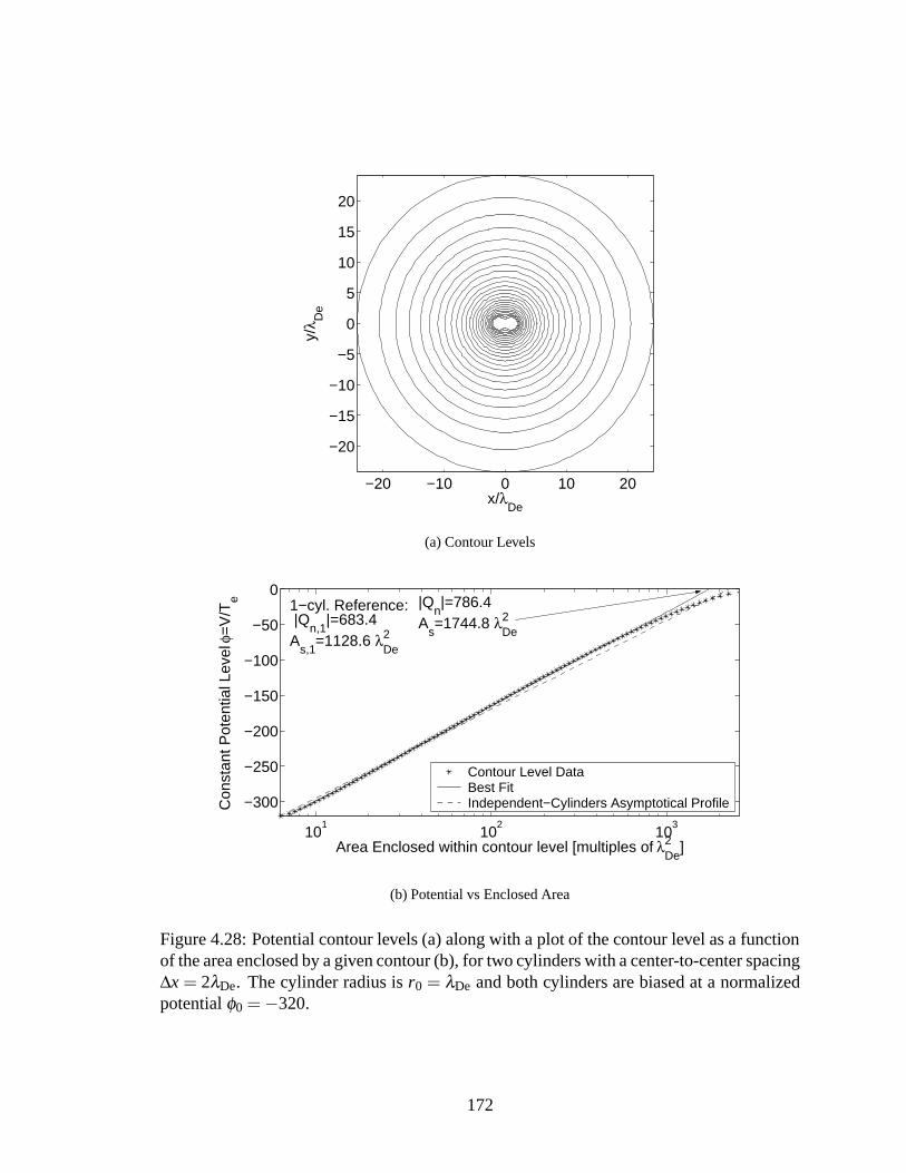
−20 −10 0 10 20
−20
−15
−10
−5
0
5
10
15
20
x/λDe
y/λ D
e
(a) Contour Levels
101
102
103
−300
−250
−200
−150
−100
−50
0
Area Enclosed within contour level [multiples of λDe2 ]
Con
stan
t Pot
entia
l Lev
el φ
=V
/Te 1−cyl. Reference:
|Qn,1
|=683.4A
s,1=1128.6 λ
De2
|Qn|=786.4
As=1744.8 λ
De2
Contour Level DataBest FitIndependent−Cylinders Asymptotical Profile
(b) Potential vs Enclosed Area
Figure 4.28: Potential contour levels (a) along with a plot of the contour level as a functionof the area enclosed by a given contour (b), for two cylinders with a center-to-center spacing∆x = 2λDe. The cylinder radius is r0 = λDe and both cylinders are biased at a normalizedpotential φ0 =−320.
172

−20 −10 0 10 20
−20
−10
0
10
20
x/λDe
y/λ D
e
(a) Contour Levels
101
102
103
−300
−250
−200
−150
−100
−50
0
Area Enclosed within contour level [multiples of λDe2 ]
Con
stan
t Pot
entia
l Lev
el φ
=V
/Te 1−cyl. Reference:
|Qn,1
|=683.4A
s,1=1128.6 λ
De2
|Qn|=1052.5
As=2244.6 λ
De2
As,virtual
=24435.2 λDe2
Contour Level DataBest FitIndependent−Cylinders Asymptotical Profile
(b) Potential vs Enclosed Area
Figure 4.29: Potential contour levels (a) along with a plot of the contour level as a functionof the area enclosed by a given contour (b), for two cylinders with a center-to-center spacing∆x= 10λDe. The cylinder radius is r0 = λDe and both cylinders are biased at a normalizedpotential φ0 =−320.
173

−20 −10 0 10 20
−20
−15
−10
−5
0
5
10
15
20
x/λDe
y/λ D
e
(a) Contour Levels
101
102
103
−300
−250
−200
−150
−100
−50
0
Area Enclosed within contour level [multiples of λDe2 ]
Con
stan
t Pot
entia
l Lev
el φ
=V
/Te 1−cyl. Reference:
|Qn,1
|=683.4A
s,1=1128.6 λ
De2
|Qn|=1287.7
As=2274.6 λ
De2
As,virtual
=4271.6 λDe2
Contour Level DataBest FitIndependent−Cylinders Asymptotical Profile
(b) Potential vs Enclosed Area
Figure 4.30: Potential contour levels (a) along with a plot of the contour level as a functionof the area enclosed by a given contour (b), for two cylinders with a center-to-center spacing∆x= 20λDe. The cylinder radius is r0 = λDe and both cylinders are biased at a normalizedpotential φ0 =−320.
174

−30 −20 −10 0 10 20 30
−10
0
10
x/λDe
y/λ D
e
(a) Contour Levels
101
102
103
−300
−250
−200
−150
−100
−50
0
Area Enclosed within contour level [multiples of λDe2 ]
Con
stan
t Pot
entia
l Lev
el φ
=V
/Te 1−cyl. Reference:
|Qn,1
|=683.4A
s,1=1128.6 λ
De2
|Qn|=1512.3
As=1377.6 λ
De2
Contour Level DataBest FitIndependent−Cylinders Asymptotical Profile
(b) Potential vs Enclosed Area
Figure 4.31: Potential contour levels (a) along with a plot of the contour level as a functionof the area enclosed by a given contour (b), for two cylinders with a center-to-center spacing∆x= 40λDe. The cylinder radius is r0 = λDe and both cylinders are biased at a normalizedpotential φ0 =−320.
175

−50 0 50
−10
0
10
x/λDe
y/λ D
e
(a) Contour Levels
101
102
103
−300
−250
−200
−150
−100
−50
0
Area Enclosed within contour level [multiples of λDe2 ]
Con
stan
t Pot
entia
l Lev
el φ
=V
/Te 1−cyl. Reference:
|Qn,1
|=683.4A
s,1=1128.6 λ
De2
|Qn|=1487.9
As=1530.3 λ
De2
Contour Level DataBest FitIndependent−Cylinders Asymptotical Profile
(b) Potential vs Enclosed Area
Figure 4.32: Potential contour levels (a) along with a plot of the contour level as a functionof the area enclosed by a given contour (b), for two cylinders with a center-to-center spacing∆x= 80λDe. The cylinder radius is r0 = λDe and both cylinders are biased at a normalizedpotential φ0 =−320.
176

−50 0 50
−100
10
x/λDe
y/λ D
e
(a) Contour Levels
101
102
103
−300
−250
−200
−150
−100
−50
0
Area Enclosed within contour level [multiples of λDe2 ]
Con
stan
t Pot
entia
l Lev
el φ
=V
/Te 1−cyl. Reference:
|Qn,1
|=683.4A
s,1=1128.6 λ
De2
|Qn|=1471.7
As=1628.8 λ
De2
Contour Level DataBest FitIndependent−Cylinders Asymptotical Profile
(b) Potential vs Enclosed Area
Figure 4.33: Potential contour levels (a) along with a plot of the contour level as a functionof the area enclosed by a given contour (b), for two cylinders with a center-to-center spacing∆x= 160λDe. The cylinder radius is r0 = λDe and both cylinders are biased at a normalizedpotential φ0 =−320.
177

followed by a “tail” attributed to space charge effects, as was seen in the single-cylinder
case. The effective sheath area corresponding to the graphed asymptote is larger than that
of a single cylinder, for which the φ -vs-A would have fallen logarithmically immediately
starting at the cylinder’s surface. In the present case, the physical extent of the touching
cylinders is sufficiently large to allow them to hold a larger total surface charge than a sin-
gle cylinder would at that same bias potential, resulting in a 55% increase of the effective
sheath size over that of a single cylinder:
As
As,1=
1744.8λ 2De
1128.6λ 2De
≈ 1.55. (4.25)
The effective sheath area is however smaller than the combined sheath area of two inde-
pendent cylinders.
Upon increasing the center-to-center spacing to ∆x = 10, as shown in Figure 4.29, the
semilog graph of the φ -vs-A data now shows two distinct linear regions, indicated by sep-
arate linear “best fits”. The first linear region (on the left) corresponds to the set of circular
contour levels enclosing each cylinder separately. The slope associated with this first region
is not as steep as that which would be expected of an independent cylinder, and is consistent
with the observed lower amount of normalized surface charge Qn held separately by each
of the cylinders as compared with the surface charge held by an independent cylinder.16
This lower charge can be attributed to a “virtual” effective sheath edge enclosing an area
As,virtual (shown on the figure to be further out on the right of the graph) that is much larger
than the effective sheath area of an independent cylinder. The fact that each cylinder holds
a lower amount of surface charge than an independent cylinder is consistent with the large
area As,virtual, as is evidenced by the following equation applicable to coaxial capacitors:
Qn,1 = 4πφ0
ln(As,1/A0), (4.26)
16Note that even though the surface charge Qn = 1052.5 shown in Figure 4.29 is larger than the surfacecharge held by an independent cylinder Q n,1= 683.4, the amount of charge held individually by each cylinder,12 Qn = 526.25, is lower.
178

where Qn,1 is the normalized surface charge held by a cylinder and A0 = πr20 is the single-
cylinder area. The expression given by (4.26) clearly shows that the surface charge Qn,1
goes down with increasing sheath area As.
The leftmost linear region extends until we approach a critical point where the equipo-
tential contours of both cylinders connect together to form a single contiguous contour. The
φ -vs-A data then rapidly switches to the rightmost linear region corresponding to the set of
circular contour levels enclosing both cylinders. The effective sheath area of the system is
defined as the A-intercept of the rightmost linear fit. In this particular case, it turns out that
the sheath area As is almost exactly equal to the combined sheath areas of two independent
cylinders, i.e., As ≈ 2As,1.
Space charge effects can be seen at two different locations in Figure 4.29. The first one
occurs near the inflection point between both linear regimes, where the φ -vs-A data is seen
to momentarily drop below the leftmost linear best-fit before it starts growing faster toward
the rightmost linear best-fit. This momentary slope reduction is attributed to the shielding
effect of space charge, which is having a detectable effect because of the sufficient spacing
between the cylinders, where some space charge exists. Beyond the turning point of this
graph, the effect of space charge becomes negligible again for a large portion of this outer
sheath, until we reach beyond an area A ≈ 1000λ 2De, where we notice the typical tail-like
behavior of the potential associated with space charge shielding.
For a center-to-center spacing of ∆x = 20λDe, we still observe two linear regimes, as
seen in Figure 4.30. The inflection point between both linear regions now occurs at a much
larger area, in the vicinity of A= 500λ 2De. The system capacitance has increased such that
the total amount of charge held by both cylinders is now almost equal to that held by two
completely independent cylinders, i.e., Qn2Qn,1∼= 0.94. This explains why the slope of the first
linear region has gotten closer to the dashed line which applies to 2 fully independent cylin-
179
ders. One might observe that the effective area As is essentially unchanged from that seen
in the case where ∆x= 10λDe, in spite of the significant increase of the surface charge held
by the cylinders. This apparent contradiction is resolved when one considers the “virtual”
effective sheath area As,virtual, which relates to the potential drop in close proximity of each
cylinder, and is much lower for ∆x= 20λDe as compared to the ∆x= 10λDe case, consistent
with the observed increase in capacitance and with (4.26) as applied to each cylinder taken
separately.
The results for a center-to-center spacing of ∆x = 40λDe are shown in Figure 4.31.
Interestingly, the total sheath area is now a smaller fraction of the independent-cylinder
sheath area: As2As,1∼= 0.61. This is consistent with the fact that the system capacitance has
gone above the combined capacitance of two single independent cylinders, i.e., Qn2Qn,1
∼=
1.11. This reduced sheath area is explained by the ion density increase on the outermost
side of each cylinder, as explained earlier in Section 4.3.3.
The results shown in Figures 4.32 and 4.33, which apply to ∆x = 80λDe and ∆x =
160λDe, correspond to a regime where both sheaths have become “Poisson-uncoupled“
while still being “Vlasov-coupled”. What we mean by this is that the charges present
in one sheath do not significantly contribute to the fields in the other sheath (“Poisson-
uncoupled”), but shadow effects and asymmetry-induced effects on unpopulated orbits
(discussed in Section 4.3.3) create connections between both sheaths (“Vlasov-coupled”).
Results for both of these spacings show that in both cases the cylinders hold a total surface
charge slightly above the surface charge that would be held by two independent cylinders,
and that their total sheath area is correspondingly slightly smaller than the total sheath area
created by two independent cylinders.
180

20 40 60 80 100 120 140 160 180 200
1.2
1.4
1.6
1.8
2
Effective Sheath Area Ratio
Center−to−Center Spacing, ∆ x/λDe
Rat
io o
f Tot
. She
ath
Are
a to
1−
Wire
She
ath
Are
a
Figure 4.34: Effective sheath area ratio as a function of the center-to-center spacing oftwo parallel cylinders. The results shown here apply to the case of two cylinders of radiusr0 = λDe with normalized bias φ0 =−320. The effective sheath area ratio is the ratio of thetwo-cylinder sheath area to the single-cylinder sheath area.
4.3.6 Parametric Analysis of the Sheath Structure
Using the definitions given in the previous section, we can now consider an analysis of
the effects of center-to-center spacing on the effective sheath area and total surface charge
held by the cylinders.
First we define the effective sheath area ratio as the ratio of the total effective sheath
area As of a two-cylinder system to the effective sheath area As,1 of a single independent
cylinder, i.e.,
RAs ≡As
As,1. (4.27)
Figure 4.34 depicts the variation of the effective sheath area ratio RAs as a function of the
center-to-center spacing ∆x of the two parallel cylinders.
The leftmost data point in Figure 4.34 corresponds to a spacing of ∆x = 2λDe and
181

applies to “touching” cylinders since they both have a radius r0 = λDe. RAs is seen to start
at about 1.55 when the cylinders are touching, indicating a total sheath area 55% larger than
that of a single cylinder. For a smaller cylinder radius, we would expect to obtain RAs = 1
when the cylinders are touching because the full extent of the two touching cylinders would
be small enough for the shadowing effect to be negligible on the density of outward-moving
ions throughout the sheath (see a discussion on this topic in Section 4.2.5).
The ratio RAs rises above 2.0 for spacings of ∆x = 5λDe and ∆x = 20λDe, indicating
that the effective sheath area is on par with the sheath area expected of two independent
cylinders. This represents an optimal spacing for purposes of maximizing the total sheath
area, as is desired for the high-energy particle precipitation application. The ratio RAs then
drops sharply to a minimum value at a spacing of about ∆x = 40λDe, and goes back up
relatively quickly until the spacing reaches ∆x = 60λDe, beyond which it follows a slow
upward slope for the remainder of the graph. It is seen that the total effective sheath area
has only reached about 1.5 times the sheath area of a single independent cylinder at a
spacing of ∆x= 200λDe, whereas we expect it to reach a ratio RAs = 2.0 when the spacing
is sufficient for the two sheaths to be fully independent of each other. An extrapolation of
a linear fit performed on this slow increase indicates that “full independence” would only
be reached at an approximate spacing ∆x ≈ 660λDe, which corresponds to about 35 times
the independent cylinder sheath radius of Rs ≈ 19λDe.
An alternative measure of the sheath dimensions can be obtained by considering the
“outward” effective sheath radius, which is measured from the center of the rightmost
cylinder toward increasing values of x on the x axis. This radius is determined based on the
cross section of the potential, consistent with the effective sheath concept used for single
cylinders. Figure 4.35 shows a plot of the ratio of the outward effective sheath radius to
the effective sheath radius of a single independent cylinder as a function of the center-to-
182
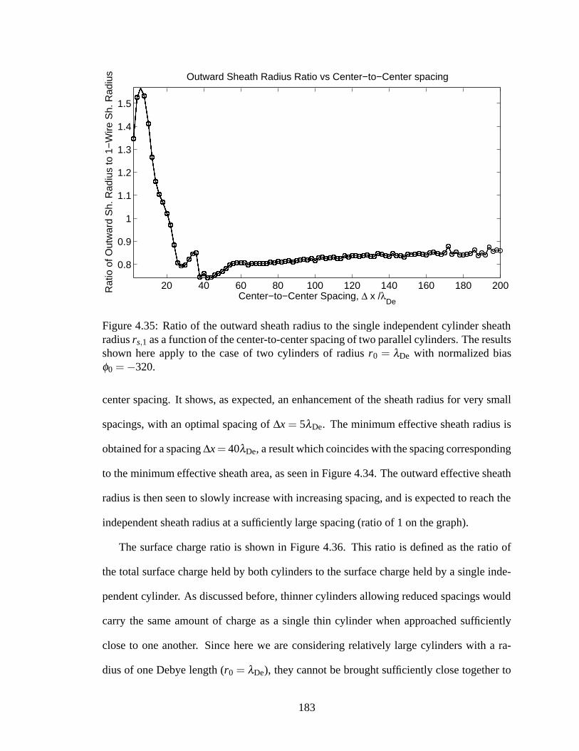
20 40 60 80 100 120 140 160 180 200
0.8
0.9
1
1.1
1.2
1.3
1.4
1.5
Outward Sheath Radius Ratio vs Center−to−Center spacing
Center−to−Center Spacing, ∆ x /λDe
Rat
io o
f Out
war
d S
h. R
adiu
s to
1−
Wire
Sh.
Rad
ius
Figure 4.35: Ratio of the outward sheath radius to the single independent cylinder sheathradius rs,1 as a function of the center-to-center spacing of two parallel cylinders. The resultsshown here apply to the case of two cylinders of radius r0 = λDe with normalized biasφ0 =−320.
center spacing. It shows, as expected, an enhancement of the sheath radius for very small
spacings, with an optimal spacing of ∆x = 5λDe. The minimum effective sheath radius is
obtained for a spacing ∆x= 40λDe, a result which coincides with the spacing corresponding
to the minimum effective sheath area, as seen in Figure 4.34. The outward effective sheath
radius is then seen to slowly increase with increasing spacing, and is expected to reach the
independent sheath radius at a sufficiently large spacing (ratio of 1 on the graph).
The surface charge ratio is shown in Figure 4.36. This ratio is defined as the ratio of
the total surface charge held by both cylinders to the surface charge held by a single inde-
pendent cylinder. As discussed before, thinner cylinders allowing reduced spacings would
carry the same amount of charge as a single thin cylinder when approached sufficiently
close to one another. Since here we are considering relatively large cylinders with a ra-
dius of one Debye length (r0 = λDe), they cannot be brought sufficiently close together to
183

20 40 60 80 100 120 140 160 180 200
1.2
1.4
1.6
1.8
2
2.2
Surface Charge Ratio
Center−to−Center Spacing, ∆ x/λDe
Rat
io o
f Sur
f. C
harg
e to
Sin
gle−
Wire
Sur
f. C
harg
e
Figure 4.36: Ratio of the total surface charge on both cylinders to the surface charge heldby a single independent cylinder. The results shown here apply to the case of two cylindersof radius r0 = λDe with normalized bias φ0 =−320.
achieve as low a capacitance as a single wire. This is why the graph shown in Figure 4.36
starts above 1.0, at a ratio of about 1.15 for a spacing ∆x = 2λDe. As the cylinders are
spaced apart, their combined capacitance increases so that the amount of charge they hold
grows to a value of about 2.25 times the single-wire surface charge at ∆x= 40λDe. This is
actually more than two independent cylinders could hold (2.0), and is consistent with the
observed reduced effective sheath area seen in Figure 4.34 as compared to the total sheath
area of two independent cylinders. The total charge then slowly ramps down as the spacing
increases beyond ∆x= 40λDe, and the graphed ratio should eventually reach 2.0.
Figure 4.37 is an alternative representation of the information shown in Figure 4.34.
It shows the “equivalent bias potential” for a single cylinder. This is the bias potential
required on a single cylinder to generate an effective sheath area equal to that generated by
our two-cylinder system biased at φ0 =−320Te. It is seen that one could create a sheath as
184

20 40 60 80 100 120 140 160 180 200
400
450
500
550
Equivalent Probe Bias vs Center−to−Center Spacing
Center−to−Center Spacing, ∆ x /λDe
φ eq
Figure 4.37: Equivalent bias potential of a single cylinder as a function of the center-to-center spacing of two parallel cylinders. The results shown here apply to the case of twocylinders of radius r0 = λDe with normalized bias φ0 =−320. The equivalent bias potentialis that which would be necessary for a single cylinder to yield the same sheath area as thecombination of the two cylinders.
large as that which is created by a single cylinder of radius r0 = λDe biased at φ0 =−570Te
by using two cylinders of equal radius r0 = λDe biased at φ0 =−320Te and spaced 5λDe or
20λDe apart.
Figure 4.38 is another alternative representation of the same information. It shows the
“equivalent radius” of the two-cylinder system as a function of center-to-center spacing.
This is the cylinder radius r0 required of a single cylinder biased at the same bias potential
φ0 = −320Te to generate the same equivalent sheath area as that generated by the two-
cylinder system. At the optimal spacings ∆x= 5λDe and ∆x= 20λDe, the equivalent radius
is about 2.85λDe.
185
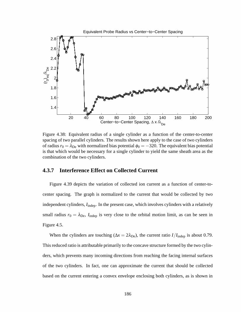
20 40 60 80 100 120 140 160 180 200
1.4
1.6
1.8
2
2.2
2.4
2.6
2.8
Equivalent Probe Radius vs Center−to−Center Spacing
Center−to−Center Spacing, ∆ x /λDe
(r0) eq
/λD
e
Figure 4.38: Equivalent radius of a single cylinder as a function of the center-to-centerspacing of two parallel cylinders. The results shown here apply to the case of two cylindersof radius r0 = λDe with normalized bias potential φ0 =−320. The equivalent bias potentialis that which would be necessary for a single cylinder to yield the same sheath area as thecombination of the two cylinders.
4.3.7 Interference Effect on Collected Current
Figure 4.39 depicts the variation of collected ion current as a function of center-to-
center spacing. The graph is normalized to the current that would be collected by two
independent cylinders, Iindep. In the present case, which involves cylinders with a relatively
small radius r0 = λDe, Iindep is very close to the orbital motion limit, as can be seen in
Figure 4.5.
When the cylinders are touching (∆x = 2λDe), the current ratio I/Iindep is about 0.79.
This reduced ratio is attributable primarily to the concave structure formed by the two cylin-
ders, which prevents many incoming directions from reaching the facing internal surfaces
of the two cylinders. In fact, one can approximate the current that should be collected
based on the current entering a convex envelope enclosing both cylinders, as is shown in
186
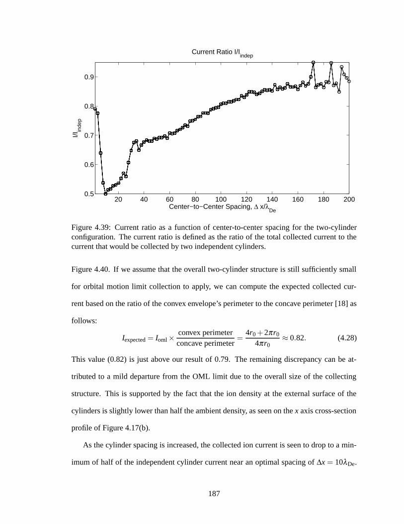
20 40 60 80 100 120 140 160 180 2000.5
0.6
0.7
0.8
0.9
Current Ratio I/Iindep
Center−to−Center Spacing, ∆ x/λDe
I/Iin
dep
Figure 4.39: Current ratio as a function of center-to-center spacing for the two-cylinderconfiguration. The current ratio is defined as the ratio of the total collected current to thecurrent that would be collected by two independent cylinders.
Figure 4.40. If we assume that the overall two-cylinder structure is still sufficiently small
for orbital motion limit collection to apply, we can compute the expected collected cur-
rent based on the ratio of the convex envelope’s perimeter to the concave perimeter [18] as
follows:
Iexpected = Ioml×convex perimeterconcave perimeter
=4r0+2πr0
4πr0≈ 0.82. (4.28)
This value (0.82) is just above our result of 0.79. The remaining discrepancy can be at-
tributed to a mild departure from the OML limit due to the overall size of the collecting
structure. This is supported by the fact that the ion density at the external surface of the
cylinders is slightly lower than half the ambient density, as seen on the x axis cross-section
profile of Figure 4.17(b).
As the cylinder spacing is increased, the collected ion current is seen to drop to a min-
imum of half of the independent cylinder current near an optimal spacing of ∆x = 10λDe.
187

Concave Perimeter
Convex Envelope
Figure 4.40: Illustration of the convex envelope surrounding both cylinders. The currentcollection to the concave portion of the perimeter is limited to some directions.
The current then rises sharply at a spacing ∆x= 30λDe, when two separate sheaths have be-
gun to form. The remainder of the graph shows a rather steady increase of collected current
with increasing spacing. This steady increase occurs once the sheaths have completely sep-
arated and are primarily coupled through the empty ion orbits connecting both cylinders’
surfaces. The observed current increase is attributed to the gradual reduction of the number
of connected ion orbits, which are not populated and therefore do not contribute current at
the cylinders’ surfaces. It is interesting to note that a similar observation was made in Sec-
tion 3.6 concerning the experimentally measured current collected by slotted tape samples.
The correlation between the experimentally observed decrease in the collection efficiency
of the perpendicular slotted tapes with increasing gap widths and our simulation results
indicate that the gap spacings sampled during our experiments were all located on the left
of the expected minimum point on the current-vs-spacing graph.
188

4.4 Solid Tape Cylinder in Stationary Plasma: CurrentCollection
The solid tape geometry is of interest primarily for the spacecraft propulsion application
of electrodynamic tethers. This geometry presents a few advantages over that of the circular
cylinder wire:
• the orbital-motion-limited regime has been shown to hold for tape widths twice that
of round cylinders, resulting in a maximum OML current collection 27% higher [11];
• a tape geometry is both lighter and more flexible [11];
• a wider tape structure would allow for improved collision survivability with orbiting
debris.
In this section we consider the current collection capability of the solid tape geometry.
The calculations were performed for electron-attracting bias potentials, but the normalized
collected currents are equally applicable to ion-attracting bias potentials. In the following,
we first make some comparisons with theoretical predictions given by Sanmartın et al [11]
and Estes and Sanmartın [12], and then compare our simulation results with experimental
data shown in Chapter 3.
4.4.1 Equivalent Cylinder Radius and Collected Current: TheoreticalComparisons
Using asymptotic analyses for both the circular cylinder and tape cylinder, Sanmartın
and Estes [11] have identified a simple relationship between the tape width w and equivalent
circular cylinder radius Req, given by Req=w4 for sufficiently thin tapes where the thickness
does not play a significant role. Their asymptotic analysis shows that, at a sufficiently large
distance from the surface of a thin tape of width w but well within the Laplace-potential
189

region,17 the potential structure varies identically as in the vicinity of a circular cylinder of
radius Req =w4 , that is,
φ ≈ φ0
[1−α1 ln
rReq
], (4.29)
where α1=Cn2π is a function of the normalized linear capacitance Cn =Qn/φ0, and Qn is the
normalized linear charge held at the surface of the cylinder. Recall that we had identified
the same asymptotic form in (4.13) based on our numerical simulations and had chosen to
write α1 in terms of an effective sheath radius rs, α1 =1
ln(rs/Req).
For a given bias potential φ0, α1 simply relates to the normalized linear charge Qn
located on the cylinder’s surface. Thus, the identification process that has led to the result
Req =w4 obtained by Sanmartın et al [11] is equivalent to finding the cylinder radius Req
that would hold the same amount of linear charge Qn as a solid tape of width w for a given
bias potential φ0.
We may therefore independently determine an equivalent radius based on equal linear
charge Qn that is equivalent to the method used by Sanmartın et al [11], but is based on our
consistent kinetic simulation results for tape and circular cylinder collectors. Figure 4.41
shows a comparison between the equal-charge probe radius as determined from our simu-
lation results and the equivalent probe radius predicted by Sanmartın et al [11]. These sim-
ulations were performed with a bias φ0= 300 and tape widths spanning from 1 to 50 Debye
lengths. Our results show a somewhat larger equivalent radius than predicted by Sanmartın
et al [11]. A best-fit linear relationship extracted from our simulation data and shown on the
legend indicates an equivalent radius Req ≈ 0.29w. The small discrepancy between these
results is most likely due to the approximations used by Sanmartin and Estes [11] in calcu-
lating the electron space charge using an asymptotic approach that does not provide a fully
17For a cylinder (of any cross-section) biased at a large potential, we define the Laplace-potential regionas the region in the immediate vicinity of the cylinder in which space charge effects do not have significanteffects on the potential profile.
190
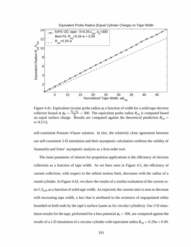
5 10 15 20 25 30 35 40 45
2
4
6
8
10
12
14
Normalized Tape Width, w/λDe
Equ
ival
ent R
adiu
s R
eq/λ
De
Equivalent Probe Radius (Equal Cylinder Charge) vs Tape Width
KiPS−2D, tape : h=0.25 λDe
, φ0=300
Best Fit: Req
=0.29 w + 0.09R
eq=0.25 w
Figure 4.41: Equivalent circular probe radius as a function of width for a solid tape electroncollector biased at φ0 =
V0−VpTe= 300. The equivalent probe radius Req is computed based
on equal surface charge. Results are compared against the theoretical prediction Req =w/4 [11].
self-consistent Poisson–Vlasov solution. In fact, the relatively close agreement between
our self-consistent 2-D simulation and their asymptotic calculation confirms the validity of
Sanmartın and Estes’ asymptotic analysis as a first-order tool.
The main parameter of interest for propulsion applications is the efficiency of electron
collection as a function of tape width. As we have seen in Figure 4.5, the efficiency of
current collection, with respect to the orbital motion limit, decreases with the radius of a
round cylinder. In Figure 4.42, we show the results of a similar evaluation of the current ra-
tio I/Ioml as a function of solid tape width. As expected, the current ratio is seen to decrease
with increasing tape width, a fact that is attributed to the existence of unpopulated orbits
bounded on both ends by the tape’s surface (same as for circular cylinders). Our 2-D simu-
lation results for the tape, performed for a bias potential φ0= 300, are compared against the
results of a 1-D simulation of a circular cylinder with equivalent radius Req= 0.29w+0.09.
191

5 10 15 20 25 30 35 40 45
0.4
0.5
0.6
0.7
0.8
0.9
1
Normalized Tape Width, w/λDe
I/Iom
l
Current Ratio I/Ioml
KiPS−2D, tape : h=0.25 λDe
, φ0=300
KiPS−1D, Req
=0.29 w+0.09, φ0=300
Figure 4.42: Current ratio I/Ioml as a function of tape width for a solid tape biased atφ0 =
V0−VpTe= 300. KiPS-2D simulation results for the tape are compared against KiPS-1D
simulation results based on the equal-charge equivalent radius determined in Figure 4.41.
The comparison clearly shows that a tape current collector has a lesser current-collection
efficiency than its equal-charge circular counterpart. From the same graph, one finds that
the maximum width of a thin tape for the OML current expression to hold within about
1% is approximately wmax ≈ 2.5λDe, which is just shy of the maximum width predicted by
Sanmartın and Estes [11] at this bias potential. 18
4.4.2 Collected Current: Comparisons with Experimental Results
Here we consider comparisons of our simulation results with some of the experimental
data pertaining to solid tapes that were shown in Chapter 3.
Figure 4.43 shows a plot of the current ratio I/Ioml, similar to that shown in Figure 4.42
but pertaining to a lower bias potential, φ0 = 100. Our simulation results are compared
against three different sets of experimental data which were obtained at three distances
18According to Sanmartın and Estes. [11, Figure 6], w max = 4Rmax ≈ 4×0.75λDe= 3λDe.
192

0 5 10 15 20 25 30 35 40 45 500.2
0.3
0.4
0.5
0.6
0.7
0.8
0.9
1
Current Ratio I/Ioml
Normalized Tape Width, w/λDe
I/Iom
l
KiPS−2D, tape : h=0.25 λDe
, φ0=100
Exp. Data, Parallel Tape, 75 cmExp. Data, Parallel Tape, 160 cmExp. Data, Parallel Tape, 300 cm
Figure 4.43: Simulated current ratio I/Ioml as a function of tape width for a solid tape biasedat φ0 =
V0−VpTe= 100, along with experimental data. Simulations were done assuming a
thin tape with finite thickness h = 0.25λDe. Simulation results are compared against ourexperimental results (detailed in Chapter 3) obtained for a solid tape at three test locationsfrom the plasma source: 75 cm (mostly flowing plasma), 160 cm and 300 cm (mostlystationary plasma). Note that the experimental data was calibrated using the round cylinderreference probe data instead of Ioml, in order to remove any flow enhancement effects forthis comparison.
from a high-speed plasma source (see details in Chapter 3): 75 cm, 160 cm, and 300cm.
Since these experiments were performed in a flowing plasma, we have attempted to “nor-
malize out” any flow enhancement factors in order to compare with our stationary simu-
lation results. Thus, instead of being normalized to the orbital-motion-limit current Ioml,
the experimental data curves shown in Figure 4.43 are normalized to the reference cylinder
data. In other words, we have plotted the following ratio in Figure 4.43 for the experimental
data curves:
Ratio≡Itape/Itape,thermal
Irefcyl/Irefcyl,thermal. (4.30)
Note that the reference cylinder is sufficiently thin to collect current at the OML level in a
193

stationary plasma.
We observe a general qualitative agreement of the data with our simulation results at
all 3 locations (75 cm, 160 cm, and 300 cm). We note that the experimental error in the
determination of the ambient density and electron temperature could explain the existing
discrepancies. Error boxes are shown in Figure 4.43 for the normalized experimental data.
The sizes of these error boxes are determined based on three types of error sources:
1. current and voltage measurement errors on the tape samples themselves, which are
estimated to amount to less than 1%;
2. systematic errors associated with the finite accuracy of the plasma parameters used
as part of the normalization process. The plasma density n0 and temperature Te,
obtained from our Langmuir Probe sweeps, were estimated to have 8% and 5% ac-
curacy, respectively, as discussed in Appendix F;
3. a systematic error associated with the finite accuracy of the total tape sample electron-
collecting area Ap, which is estimated to be on the order of 6%, similiar to the error
on the Langmuir probe area discussed in Appendix F.
So, using the 8% and 5% error estimates for density and temperature, we can infer a 6.5%
error on the Debye length, since λDe ∝√
Te/n0. Now, since Ioml is proportional to n0×
Ap×√
V , where V is the applied tether voltage and Ap is the total area of the tape sample,
the 1% error on voltage measurements and 6% error on tape area Ap combine with the 8%
error on density to yield for Ioml an error of 8%+ 6%+ 0.5 ∗ 1%= 14.5%. Therefore, in
Figure 4.43, the error boxes surrounding the normalized data points have a relative height
of 1%+14.5%=15.5%, corresponding to the sum of the error on measured current I and
the error on Ioml , and a relative width of 6.5% corresponding to the relative error on the
normalized width w/λDe, where we assume that the bulk of the error is contributed by
194

the error on λDe while the actual widths w have a much better precision due to use of an
electrical discharge machining process for tape sample fabrication.
Having first observed the dependence of collected current on tape width, we now con-
sider the complete current characteristics (Current vs Voltage) of several tape configura-
tions, which we compare against our experimental results. Figures 4.44 through 4.46 show
the simulation/experiment comparisons pertaining to the three sample positions that were
tested: 75 cm, 160 cm and 300 cm from the plasma source (see Chapter 3 for details).
Only the parallel tape data were used, since they featured less flow effects than the
perpendicular tape data and were therefore more appropriate for comparison with our sta-
tionary plasma computer simulations. It should be emphasized that the experimental data
were processed in such a way as to remove the remaining flow effects. This was done
by multiplying all normalized tape current data by the ratio of the normalized reference
cylinder data Irefcyl/Irefcyl,thermal to the theoretical normalized OML current Ioml:
Iwithout flow(V )≈ Iwith flow(V )×Ioml(V )
Irefcyl(V )/Irefcyl,thermal(V ). (4.31)
This is thought to remove much of the flow-induced current enhancement, since the refer-
ence cylinder experiences a similar enhancement. However, we must still keep in mind that
some of the flow enhancement could still be present in the experimental data, especially at
the closest range of 75 cm, since the correction above is only approximate. At the farthest
range however (300 cm) we have determined that the plasma was mostly stationary, and
therefore the normalization performed by (4.31) only had a minor effect.
The simulation and experimental results shown in Figures 4.44 through 4.46 are in good
agreement for the widest tape configuration, whereas for the medium and narrow tapes the
experimental data is less efficient than predicted by our simulations. The reduction of the
current collection efficiency caused by the screw attachments is thought to be the most
likely cause for this discrepancy, since the fraction of the collecting area contributed by the
195

0 20 40 60 80 100 120
2
4
6
8
10
12
14
16
Normalized Bias Potential φ0=(V
0−V
p)/T
e
Nor
mal
ized
Ele
ctro
n C
urre
nt I e/I th
e
Electron Current Characteristic, Tape Cylinder
OML LimitKiPS−2D , w=13.7λ
De, h=0.7 λ
DeKiPS−2D , w=20.4λ
De, h=0.7 λ
DeKiPS−2D , w=41.9λ
De, h=0.7 λ
DeExp. Data, w=13.7λ
De, h=0.7λ
De (75 cm)
Exp. Data, w=20.4λDe
, h=0.7λDe
(75 cm)Exp. Data, w=41.9λ
De, h=0.7λ
De (75 cm)
Figure 4.44: Normalized current characteristics of solid tapes: comparison of simulationresults with experimental data obtained at 75 cm. Three different tape widths are compared.Tape widths w and thicknesses h are indicated in terms of the local Debye length.
screws is significantly more important in the case of a narrow tape than it is in the case of
a wide tape. Note that the screw areas were accounted for in the calculation of the total
sample area, as discussed in Chapter 3.
4.5 Flow Effects on Ion-Attracting Round Cylinder
We now consider the effects of plasma flow on the sheath structure and current collec-
tion of ion-attracting round cylinders. We will consider flow speeds U that are very small
with respect to the electron thermal velocity vthe, i.e., U << vthe. Therefore, the electrons
are essentially a stationary species that only respond to the asymmetries in the potential
structure. Those asymmetries are introduced by the ions, whose thermal velocity is on the
order or even slower than the flow speed U .
Throughout this section, we designate the flow speed using three alternate notations:
196

0 20 40 60 80 100 120 140 160
2
4
6
8
10
12
14
16
18
20
22
Normalized Bias Potential φ0=(V
0−V
p)/T
e
Nor
mal
ized
Ele
ctro
n C
urre
nt I e/I th
e
Electron Current Characteristic, Tape Cylinder
OML LimitKiPS−2D , w=7.4λ
De, h=0.38 λ
DeKiPS−2D , w=11λ
De, h=0.38 λ
DeKiPS−2D , w=22.6λ
De, h=0.38 λ
DeExp. Data, w=7.4λ
De, h=0.38λ
De (160 cm)
Exp. Data, w=11λDe
, h=0.38λDe
(160 cm)Exp. Data, w=22.6λ
De, h=0.38λ
De (160 cm)
Figure 4.45: Normalized current characteristics of solid tapes: comparison of simulationresults with experimental data obtained at 160 cm. Three different tape widths are com-pared. Tape widths w and thicknesses h are indicated in terms of the local Debye length.
0 20 40 60 80 100 120 140 160 180
2
4
6
8
10
12
14
16
18
20
22
Normalized Bias Potential φ0=(V
0−V
p)/T
e
Nor
mal
ized
Ele
ctro
n C
urre
nt I e/I th
e
Electron Current Characteristic, Tape Cylinder
OML LimitKiPS−2D , w=4.9λ
De, h=0.25 λ
DeKiPS−2D , w=7.2λ
De, h=0.25 λ
DeKiPS−2D , w=14.9λ
De, h=0.25 λ
DeExp. Data, w=4.9λ
De, h=0.25λ
De (300 cm)
Exp. Data, w=7.2λDe
, h=0.25λDe
(300 cm)Exp. Data, w=14.9λ
De, h=0.25λ
De (300 cm)
Figure 4.46: Normalized current characteristics of solid tapes: comparison of simulationresults with experimental data obtained at 300 cm. Three different tape widths are com-pared. Tape widths w and thicknesses h are indicated in terms of the local Debye length.
197

• the flow velocity U , given in m/s;
• the flow energy Uev, given in eV, which relates to the velocity U through the expres-
sion
Uev =miU2
2e, (4.32)
where mi is the ion atomic mass, and e= 1.6×10⁻¹⁹ C;
• the ion speed ratio Sd , which is the ratio of the flow velocity to the ion thermal
velocity, given by
Sd =Uvthi=
√Uev
Ti, (4.33)
where Ti is the ion temperature in eV. The ratio Sd is used in section 4.5.3 when
making comparisons with a publication using that notation.
In the following, we first describe the trapped orbit criteria, and the various treatments
of electrons that were used here. In Section 4.5.3, we perform a few validations with
the simulation results obtained by Xu [17]. Finally, in Section 4.5.4, we perform a detailed
analysis of the impact of the ionospheric flow on the sheath structure and ion current collec-
tion at an altitude that is representative of the high-energy particle precipitation application.
4.5.1 Criteria for Trapped Orbits
The asymmetry introduced by the plasma flow allows for the existence of some orbits
of increased complexity, although not quite as complex as in the two-cylinder case. To
accommodate for these relatively complex trajectories, we have set the maximum number
of orbits to Morb = 3, which corresponds to a maximum angular displacement of 6π (see
definition for Morb in Section 2.4.2.2) beyond which a trajectory will be deemed trapped.
A maximum number of radial oscillations was not necessary for these simulations, since it
would be redundant.
198
4.5.2 Treatment of Electrons
For similar reasons as in the case of the two-cylinder electron-repelling configuration
described in Section 4.3.1, the treatment of electrons can be greatly simplified in the present
case, because the electron population is not effectively drifting. Since in the flowing case
the potential can get slightly positive at some locations (on the ram side of the cylinder)
even when applying a negative bias potential, an accurate collisionless treatment for elec-
trons that provides excellent accuracy is based on the following “clipped” Boltzmann equa-
tion:
ne =
{n0 exp V
TeV ≤ 0
n0 V > 0.(4.34)
This treatment is actually exact for a stationary species if all collisionless orbits are con-
nected to the background plasma, which is the case here because the electrons are repelled,
implying that no electron orbit intersects the probe for all practical purposes. Using a “full
Boltzmann” approximation for electrons, i.e., setting ne = n0 exp VTe
for both negative (re-
pelling) and positive (attracting) potentials, is also appropriate as long as potentials do not
significantly exceed zero. Doing so actually provides a feedback mechanism in the simu-
lation which improves the convergence rate, and does not unduly impact the quality of the
solution as long as the final potential profile does not significantly exceed zero.
Three different types of treatments were used to compute the electron density in the
simulations presented in Section 4.5.3. They are:
Boltzmann Electrons This is the same approximation as was used by Xu [17], and is
designated above as the “full Boltzmann” approximation.
“Clipped” Boltzmann Electrons This approximation is appropriate for low speeds only.
It does not allow for any negative-energy electrons, and therefore could not be used
for some combinations of high-voltage and/or high-speed settings due to numerical
199

stability issues.
Kinetic Electrons This is the same kinetic treatment as is used for the ions, and involves
tracking thousands of trajectories in order to compute the density at a given interro-
gation point.
The last two methods, the “clipped” Boltzmann and kinetic electrons, have not reached
convergence for all combinations of voltage and speed settings, due to the non-smoothness
of the electrons’ Vlasov Jacobian matrix. For this reason and due also to time constraints,
some of the graphs shown throughout Section 4.5.3 only contain simulation data for a
subset of the three electron treatments just mentionned. All data points shown, however,
are based on adequately converged, self-consistent simulations.
4.5.3 Validation with Existing Simulation Results
Before using our model for the analysis of our application of interest, we consider some
comparisons with simulations performed by Xu [17]. Ion density profiles and collected ion
current are compared below.
4.5.3.1 Ion Density Profile Validations
Figures 4.47 and 4.48 illustrate the cross-sectional ion density profiles obtained for
various flow speeds along the axis of plasma flow (x axis) for a round conductive cylinder
(r0 = λDe) biased at a normalized potential φ0 = −25. Four different flow speed settings
are shown corresponding to speed ratios Sd = 0.5, 1, 3, and 6 or, alternatively, flow energies
Uev = 0.25Te, Te, 9Te and 36Te.
The agreement between our results and Xu’s results [17] is very good, except perhaps
for some minor discrepancies on the ram side of the cylinders at low speed (Sd = 0.5 and
1).
200

−40 −30 −20 −10 0 10 20 30 40−0.2
0
0.2
0.4
0.6
0.8
1
Ion density Profile on X axis (r0=λ
De, φ
0=−25, S
d=0.5)
x/λDe
Nor
mal
ized
Ion
dens
ity n
i/n0
KiPS−2D: Boltzmann ElectronsKiPS−2D: "Clipped" Boltzmann ElectronsKiPS−2D, Kinetic ElectronsXu[1992] (Boltzmann electrons)
−40 −30 −20 −10 0 10 20 30 40
−0.4
−0.2
0
0.2
0.4
0.6
0.8
1
Ion density Profile on X axis (r0=λ
De, φ
0=−25, S
d=1)
x/λDe
Nor
mal
ized
Ion
dens
ity n
i/n0
KiPS−2D: Boltzmann ElectronsKiPS−2D: "Clipped" Boltzmann ElectronsKiPS−2D, Kinetic ElectronsXu[1992] (Boltzmann electrons)
Figure 4.47: Ion normalized density profile along the central axis of a round conductivecylinder (r0 = λDe) biased at a potential of −25Te and immersed in a plasma flowing atspeed ratios Sd = 0.5 and Sd = 1, with corresponding flow energies of Uev = 0.25Te andUev = Te. Results are compared against the simulation results published by Xu [17], whichused the Boltzmann approximation for the electrons.
201

−30 −20 −10 0 10 20 300
0.2
0.4
0.6
0.8
1
1.2
1.4
Ion density Profile on X axis (r0=λ
De, φ
0=−25, S
d=3)
x/λDe
Nor
mal
ized
Ion
dens
ity n
i/n0
KiPS−2D: Boltzmann ElectronsXu[1992] (Boltzmann electrons)
−40 −30 −20 −10 0 10 20 30 400
0.2
0.4
0.6
0.8
1
1.2
1.4
Ion density Profile on X axis (r0=λ
De, φ
0=−25, S
d=6)
x/λDe
Nor
mal
ized
Ion
dens
ity n
i/n0
KiPS−2D: Boltzmann ElectronsKiPS−2D, Kinetic ElectronsXu[1992] (Boltzmann electrons)
Figure 4.48: Ion normalized density profile along the central axis of a round conductivecylinder (r0 = λDe) biased at a potential of −25Te and immersed in a plasma flowing atspeed ratios Sd = 3 and Sd = 6, with corresponding flow energies of Uev = 9Te and Uev =36Te. Results are compared against the simulation results published by Xu [17], whichused the Boltzmann approximation for the electrons.
202

The ion density on the ram-side surface of the cylinder is seen to stay close to the
ambient density up to a relatively close distance from the cylinder. The density then drops
to a value which, for sufficiently large flow speeds (Sd = 3 and Sd = 6), is larger than the
orbital-motion limit of half the ambient density. This is of course attributable to the average
drift velocity of the ion population. In the limit of very high speeds, practically all of the
ion population would be moving to the right at a uniform velocity and would “ram” the
cylinder without having been deflected by its surrounding electric fields, translating into a
density equal to the ambient density on the ram-side of the cylinder’s surface.
On the wake side of the cylinder, the depletion of ions due to plasma flow is seen to
occur very quickly: the wake-side surface density has already dropped to around one-fifth
of the ambient density for a speed ratio Sd = 0.5, and is zero for the three other speed
settings.
4.5.3.2 Ion Current Collection Validations
Figures 4.49 and 4.50 show some comparisons of the ion current dependence on the
flow speed ratio Sd for various probe radii: r0 = 0.2λDe, λDe, 5λDe and 10λDe. Agree-
ment between our simulation data and Xu’s results [17] is very good. Our results show a
similar departure from Godard and Laframboise’s symmetric-profile as was observed by
Xu at intermediate values of the speed ratio. However, they indicate a less pronounced
dip of the current at the critical speed corresponding to the minimum current collection.
This observation is most obvious on the lower graph in Figure 4.49 at the highest bias po-
tential setting, φ0 = −25: Xu’s data goes down to a minimum of 4.4, while our KiPS-2D
simulation results do not go much lower than 5.0.
The non-monotonic nature of these current curves can be explained by the combination
of two opposite phenomena: the decrease of the wake-side current and the increase of the
ram-side current. As the flow speed is increased from zero, the wake-side density drops
203

0 1 2 3 4 5 6 7
3
4
5
6
7
8
9
10
11
12
Normalized Ion Current vs Ion Speed Ratio, r0=0.2 λ
De
Ion Speed Ratio Sd=U/v
thi
Nor
mal
ized
Ion
Cur
rent
I i/I thi
KiPS−2D: Boltzmann ElectronsKiPS−2D: "Clipped" Boltzmann ElectronsKiPS−2D, Kinetic ElectronsXu[1992]Godard and Laframboise[1983]
φ0=−5
φ0=−15
φ0=−25
0 1 2 3 4 5 6 7
3
4
5
6
7
8
9
10
11
12
Normalized Ion Current vs Ion Speed Ratio, r0=λ
De
Ion Speed Ratio Sd=U/v
thi
Nor
mal
ized
Ion
Cur
rent
I i/I thi
KiPS−2D: Boltzmann ElectronsKiPS−2D: "Clipped" Boltzmann ElectronsKiPS−2D, Kinetic ElectronsXu[1992]Godard and Laframboise[1983]
φ0=−5
φ0=−15
φ0=−25
Figure 4.49: Collected ion current as a function of the ion speed ratio Sd , for a round con-ductive cylinder with probe radii r0 = 0.2λDe and r0 = λDe, immersed in a flowing plasmawith Ti = Te. KiPS-2D results for three different bias potentials (φ0 = −5,−15,−25) arecompared with simulation results published by Xu [17] (asymmetric profile, kinetic code)and Godard and Laframboise [30] (symmetric sheath approximation).
204

0 1 2 3 4 5 6 7
3
4
5
6
7
8
9
10
11
12
Normalized Ion Current vs Ion Speed Ratio, r0=5 λ
De
Ion Speed Ratio Sd=U/v
thi
Nor
mal
ized
Ion
Cur
rent
I i/I thi
KiPS−2D: Boltzmann ElectronsKiPS−2D: "Clipped" Boltzmann ElectronsKiPS−2D, Kinetic ElectronsXu[1992]Godard and Laframboise[1983]
φ0=−5
φ0=−15
φ0=−25
0 1 2 3 4 5 6 7
3
4
5
6
7
8
9
10
11
12
Normalized Ion Current vs Ion Speed Ratio, r0=10 λ
De
Ion Speed Ratio Sd=U/v
thi
Nor
mal
ized
Ion
Cur
rent
I i/I thi
KiPS−2D: Boltzmann ElectronsKiPS−2D: "Clipped" Boltzmann ElectronsKiPS−2D, Kinetic ElectronsXu[1992]Godard and Laframboise[1983]
φ0=−5
φ0=−15
φ0=−25
Figure 4.50: Collected ion current as a function of the ion speed ratio Sd , for a round con-ductive cylinder with probe radii r0 = 5λDe and r0 = 10λDe, immersed in a flowing plasmawith Ti = Te. KiPS-2D results for three different bias potentials (φ0 = −5,−15,−25) arecompared with simulation results published by Xu [17] (asymmetric profile, kinetic code)and Godard and Laframboise [30] (symmetric sheath approximation).
205

dramatically, as was seen on the ion density profiles shown in Figures 4.47 and 4.48. The
relatively slow increase in ram-side current collection initially does not suffice to counter
the decrease in wake-side current, which leads to a net decrease of the collected current. As
the plasma speed increases further, the wake-side current eventually reaches zero. Beyond
this point, the net current starts increasing again because its sole contribution is now the
ram-side current, which increases with the incoming beam velocity.
4.5.4 Ionospheric Flow Effects at High Altitudes (H=1500 km)
For the energetic particle precipitation application (also known as the remediation of
radiation belts), we are primarily interested in whether or not we should expect the orbital
velocity of a tether, which can be interpreted as plasma flow as seen from the frame of
reference of the tether, to affect the overall sheath dimensions and ion current collection
properties as determined for a stationary plasma in Section 4.2. For the following study,
we will consider a representative altitude of 1500 km for the operation of an electrodynamic
tether as a scattering device. If the tether were located on an equatorial orbit, placing it at
this particular altitude would allow for remediation of radiation belts in the vicinity of the
L= 1.24 magnetic field shell 19.
4.5.4.1 Flow Energy at Altitude of Interest
At an altitude of 1500 km, Hydrogen is the dominant ion species. If we assume a
circular orbit, and further assume that the orbital velocity U = 7113 m/s [80] completely
translates into plasma motion relative to the spacecraft,20 we may compute the flow energy
19The L-shell level on the equatorial plane is computed as the ratio of the distance from the Earth’s centerto the Earth’s radius. In this case, L= 1500km+6370km
6370km ≈ 1.24.20This is not rigorously accurate, since the ionosphere rotates around the Earth in the opposite direction,
somewhat reducing the net relative velocity.
206

Uev to be
Uev =miv2
2e= 0.265 eV, (4.35)
where we have used Hydrogen’s atomic mass mi = 1.67× 10⁻²⁷ kg, the orbital velocity
U = 7113 m/s, and the constant e= 1.6×10⁻¹⁹ J/eV. Since we assume for the electron and
ion temperature Ti= Te = 0.4 eV (see Table 1.1), the normalized flow energy is UevTe≈ 0.66,
and corresponds to a speed ratio Sd =√
0.66= 0.81 with respect to the ion thermal velocity.
4.5.4.2 Inspection of the Sheath Structure
In order to address the question of the importance of flow effects, we set the flow
speed at a fixed value Uev = 0.66Te and observe the changes in the structure of the plasma
as we gradually increase the bias potential on the cylinder. Figures 4.51 through 4.64
show some 2-D distributions along with corresponding x-axis cross sections of the net
charge, potential, and density distributions corresponding to cylinder bias potentials of
φ0 = −5,−10,−20,−50,−100,−200 and −300. In addition, overlays of all of the po-
tential and density cross-section profiles are provided in Figures 4.65 and 4.66. Note that
the “clipped Boltzmann” treatment was used for electrons for all these simulations.
One immediately notices that the asymmetries present at low bias potentials do not fade
away as the bias potential increases to values as large as φ0 = −300, a bias potential over
450 times the flow energy. This may be regarded as contrary to “common wisdom”, ac-
cording to which an impinging flow energy as small as UevTe= 0.66 should have a negligible
effect on the sheath structure with bias potentials a few orders of magnitude larger. As Fig-
ure 4.66 shows, the asymmetry in the ion and electron density profiles only gets stronger as
the bias potential is increased. As far as the potential profile is concerned, it only shows vis-
ible signs of asymmetry as one gets closer to the pre-sheath, with the wake-side pre-sheath
zone showing a slightly negative potential, offset from the ram-side pre-sheath potential by
207

an amount on the order of the beam energy. This “tail” in the potential profile is still clearly
visible with a bias potential φ0 =−300.
A flow energy equal to 66% of the thermal energy (Uev = 0.66Te) introduces a signifi-
cant asymmetry in the ion population’s Maxwellian velocity distribution in the background
plasma. The resulting asymmetry in the ionic density distribution causes a corresponding
asymmetry in the potential distribution, breaking the conservation of angular momentum
associated with a central force. This has two effects:
• the unpopulated trapped orbits are compressed to the right, away from the cylinder
on the wake side and closer to the cylinder on the ram side;
• the ion-depleting effect of the cylinder’s shadow becomes less important on the ram
side and more important on the wake side.
Both of these effects cause the ion density to keep to the ambient value up to a much closer
distance on the ram side of the cylinder, while stretching the depletion zone further out on
the wake side. One observes that, even though the bias potential is large, the “ion source”
feeding the high-voltage sheath is located in the background plasma, where the potential is
zero. Thus, when assessing whether asymmetries should be expected or not, the important
parameter to compare against flow energy is not the bias potential, but the ion temperature
at the source, in the background plasma. An ion source which has a significant offset (≡
flow speed) in its velocity distribution function will cause significant asymmetries in the
ionic density profiles, especially as the bias potential increases.
Another aspect of interest that is noted from the ionic density profiles is the significant
drop of the ion density on the wake side’s surface of the cylinder, down to a value near
0.15n0 for a bias potential of φ0 = −300. As we will see in what follows, this causes a
reduction of the collected current as compared to the stationary case.
208

−15 −10 −5 0 5 10 15 0
5
10
15
0
0.1
0.2
0.3
0.4
0.5
0.6
0.7
y/λ D
e
x/λDe
ρ in/(
en0)
−15 −10 −5 0 5 10 150
0.1
0.2
0.3
0.4
0.5
0.6
0.7
x/λDe
ρ in/(
e n 0)
(a) Input Net Charge Distribution ρin/(en0)
⇓ (Poisson Solver)⇓
−15 −10 −5 0 5 10 15 0
5
10
15
−5
−4
−3
−2
−1
φ
x/λDe
y/λ D
e −15 −10 −5 0 5 10 15
−4.5
−4
−3.5
−3
−2.5
−2
−1.5
−1
−0.5
x/λDe
φ=(V
−V
p)/T
e
(b) Potential Distribution φ = (V −Vp)/Te
⇓ (Vlasov Solver)⇓
−15 −10 −5 0 5 10 15 0
5
10
15
0
0.1
0.2
0.3
0.4
0.5
0.6
0.7
x/λDe
y/λ D
e
ρ out/(
en0)
−15 −10 −5 0 5 10 150
0.1
0.2
0.3
0.4
0.5
0.6
0.7
x/λDe
ρ out/(
e n 0)
(c) Output Net Charge Distribution ρout/(en0)
Figure 4.51: Poisson–Vlasov consistent solution for an ion-attracting cylinder (r0 = λDe)biased at φ0 =−5 and immersed in a flowing plasma with flow energy Uev = 0.66Te. Self-consistency is shown by the similarity of ρin and ρout. 2-D solutions are shown on the left,and corresponding x-axis cross-section profiles are shown on the right. Corresponding ionand electron density distributions are shown in Figure 4.52.
209

−15 −10 −5 0 5 10 15 0
5
10
15
0.2
0.4
0.6
0.8
y/λ D
e
x/λDe
n e/n0
−15 −10 −5 0 5 10 15
0.1
0.2
0.3
0.4
0.5
0.6
0.7
0.8
0.9
x/λDe
n e/n0
(a) Normalized Electron Number Density ne/n0.
−15 −10 −5 0 5 10 15 0
5
10
15
0.3
0.4
0.5
0.6
0.7
0.8
0.9
1
n i/n0
x/λDe
y/λ D
e
−15 −10 −5 0 5 10 15
0.3
0.4
0.5
0.6
0.7
0.8
0.9
1
x/λDe
n i/n0
(b) Normalized Ion Number Density ni/n0.
Figure 4.52: Poisson–Vlasov consistent electron and ion density distributions for an ion-attracting cylinder (r0 = λDe) biased at φ0 = −5 and immersed in a flowing plasma withflow energy Uev = 0.66Te. These density profiles constitute the output of the Vlasov solverand are subtracted to form the output net charge density profile �ρout = e(�ni−�ne) shown inFigure 4.51(c).
210
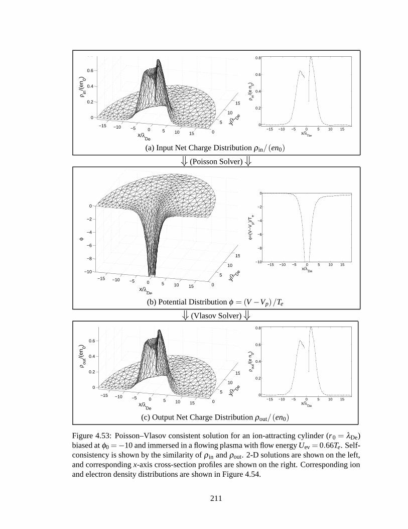
−15 −10 −5 0 5 10 15 0
5
10
15
0
0.2
0.4
0.6
0.8
ρ in/(
en0)
x/λDe
y/λ D
e
−15 −10 −5 0 5 10 150
0.2
0.4
0.6
0.8
x/λDe
ρ in/(
e n 0)
(a) Input Net Charge Distribution ρin/(en0)
⇓ (Poisson Solver)⇓
−15 −10 −5 0 5 10 15 0
5
10
15
−10
−8
−6
−4
−2
0
φ
x/λDe
y/λ D
e
−15 −10 −5 0 5 10 15−10
−8
−6
−4
−2
0
x/λDe
φ=(V
−V
p)/T
e
(b) Potential Distribution φ = (V −Vp)/Te
⇓ (Vlasov Solver)⇓
−15 −10 −5 0 5 10 15 0
5
10
15
0
0.2
0.4
0.6
0.8
ρ out/(
en0)
x/λDe
y/λ D
e
−15 −10 −5 0 5 10 150
0.2
0.4
0.6
0.8
x/λDe
ρ out/(
e n 0)
(c) Output Net Charge Distribution ρout/(en0)
Figure 4.53: Poisson–Vlasov consistent solution for an ion-attracting cylinder (r0 = λDe)biased at φ0=−10 and immersed in a flowing plasma with flow energy Uev = 0.66Te. Self-consistency is shown by the similarity of ρin and ρout. 2-D solutions are shown on the left,and corresponding x-axis cross-section profiles are shown on the right. Corresponding ionand electron density distributions are shown in Figure 4.54.
211

−15 −10 −5 0 5 10 15 0
5
10
150.2
0.4
0.6
0.8
1
n e/n0
x/λDe
y/λ D
e −15 −10 −5 0 5 10 15
0.2
0.4
0.6
0.8
1
x/λDe
n e/n0
(a) Normalized Electron Number Density ne/n0.
−15 −10 −5 0 5 10 15 0
5
10
15
0.3
0.4
0.5
0.6
0.7
0.8
0.9
1
x/λDe
y/λ D
e
n i/n0
−15 −10 −5 0 5 10 150.3
0.4
0.5
0.6
0.7
0.8
0.9
1
x/λDe
n i/n0
(b) Normalized Ion Number Density ni/n0.
Figure 4.54: Poisson–Vlasov consistent electron and ion density distributions for an ion-attracting cylinder (r0 = λDe) biased at φ0 = −10 and immersed in a flowing plasma withflow energy Uev = 0.66Te. These density profiles constitute the output of the Vlasov solverand are subtracted to form the output net charge density profile �ρout = e(�ni−�ne) shown inFigure 4.53(c).
212

−20 −10 0 10 20 0
5
10
15
20
0
0.2
0.4
0.6
0.8
y/λ D
e
x/λDe
ρ in/(
en0)
−20 −10 0 10 200
0.2
0.4
0.6
0.8
x/λDe
ρ in/(
e n 0)
(a) Input Net Charge Distribution ρin/(en0)
⇓ (Poisson Solver)⇓
−20 −10 0 10 20 0
5
10
15
20
−20
−15
−10
−5
0
y/λ D
e
x/λDe
φ
−20 −10 0 10 20−20
−15
−10
−5
0
x/λDe
φ=(V
−V
p)/T
e
(b) Potential Distribution φ = (V −Vp)/Te
⇓ (Vlasov Solver)⇓
−20 −10 0 10 20 0
5
10
15
20
0
0.2
0.4
0.6
0.8
ρ out/(
en0)
x/λDe
y/λ D
e
−20 −10 0 10 200
0.2
0.4
0.6
0.8
x/λDe
ρ out/(
e n 0)
(c) Output Net Charge Distribution ρout/(en0)
Figure 4.55: Poisson–Vlasov consistent solution for an ion-attracting cylinder (r0 = λDe)biased at φ0=−20 and immersed in a flowing plasma with flow energy Uev = 0.66Te. Self-consistency is shown by the similarity of ρin and ρout. 2-D solutions are shown on the left,and corresponding x-axis cross-section profiles are shown on the right. Corresponding ionand electron density distributions are shown in Figure 4.56.
213

−20 −10 0 10 20 0
5
10
15
200.2
0.4
0.6
0.8
1
y/λ D
e
x/λDe
n e/n0
−20 −10 0 10 20
0.2
0.4
0.6
0.8
1
x/λDe
n e/n0
(a) Normalized Electron Number Density ne/n0.
−20 −10 0 10 20 0
5
10
15
20
0.3
0.4
0.5
0.6
0.7
0.8
0.9
1
y/λ D
e
x/λDe
n i/n0
−20 −10 0 10 200.3
0.4
0.5
0.6
0.7
0.8
0.9
1
x/λDe
n i/n0
(b) Normalized Ion Number Density ni/n0.
Figure 4.56: Poisson–Vlasov consistent electron and ion density distributions for an ion-attracting cylinder (r0 = λDe) biased at φ0 = −20 and immersed in a flowing plasma withflow energy Uev = 0.66Te. These density profiles constitute the output of the Vlasov solverand are subtracted to form the output net charge density profile �ρout = e(�ni−�ne) shown inFigure 4.55(c).
214
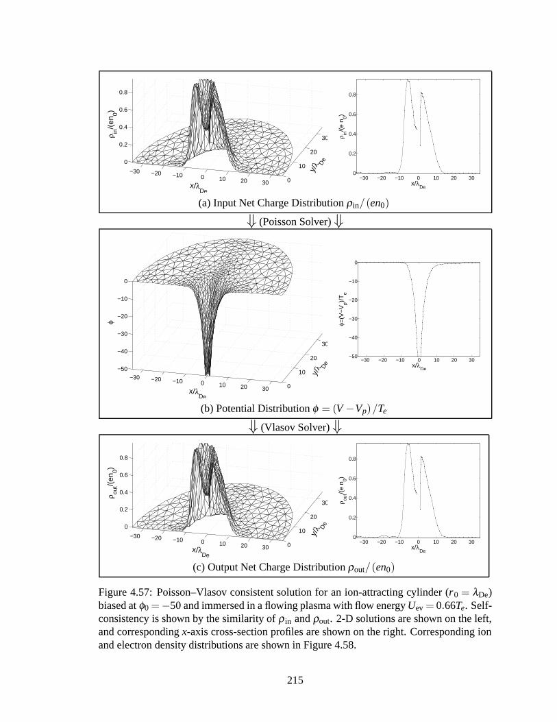
−30 −20 −10 0 10 20 30 0
10
20
30
0
0.2
0.4
0.6
0.8
x/λDe
y/λ D
e
ρ in/(
en0)
−30 −20 −10 0 10 20 300
0.2
0.4
0.6
0.8
x/λDe
ρ in/(
e n 0)
(a) Input Net Charge Distribution ρin/(en0)
⇓ (Poisson Solver)⇓
−30 −20 −10 0 10 20 30 0
10
20
30
−50
−40
−30
−20
−10
0
φ
x/λDe
y/λ D
e −30 −20 −10 0 10 20 30
−50
−40
−30
−20
−10
0
x/λDe
φ=(V
−V
p)/T
e
(b) Potential Distribution φ = (V −Vp)/Te
⇓ (Vlasov Solver)⇓
−30 −20 −10 0 10 20 30 0
10
20
30
0
0.2
0.4
0.6
0.8
1
y/λ D
e
x/λDe
ρ out/(
en0)
−30 −20 −10 0 10 20 300
0.2
0.4
0.6
0.8
x/λDe
ρ out/(
e n 0)
(c) Output Net Charge Distribution ρout/(en0)
Figure 4.57: Poisson–Vlasov consistent solution for an ion-attracting cylinder (r0 = λDe)biased at φ0=−50 and immersed in a flowing plasma with flow energy Uev = 0.66Te. Self-consistency is shown by the similarity of ρin and ρout. 2-D solutions are shown on the left,and corresponding x-axis cross-section profiles are shown on the right. Corresponding ionand electron density distributions are shown in Figure 4.58.
215

−30 −20 −10 0 10 20 30 0
10
20
300.2
0.4
0.6
0.8
1
n e/n0
x/λDe
y/λ D
e −30 −20 −10 0 10 20 30
0.2
0.4
0.6
0.8
1
x/λDe
n e/n0
(a) Normalized Electron Number Density ne/n0.
−30 −20 −10 0 10 20 30 0
10
20
30
0.3
0.4
0.5
0.6
0.7
0.8
0.9
1
n i/n0
x/λDe
y/λ D
e −30 −20 −10 0 10 20 30
0.3
0.4
0.5
0.6
0.7
0.8
0.9
1
x/λDe
n i/n0
(b) Normalized Ion Number Density ni/n0.
Figure 4.58: Poisson–Vlasov consistent electron and ion density distributions for an ion-attracting cylinder (r0 = λDe) biased at φ0 = −50 and immersed in a flowing plasma withflow energy Uev = 0.66Te. These density profiles constitute the output of the Vlasov solverand are subtracted to form the output net charge density profile �ρout = e(�ni−�ne) shown inFigure 4.57(c).
216

−40 −20 0 20 40 0
10
20
30
40
0
0.2
0.4
0.6
0.8
1
x/λDe
y/λ D
e
ρ in/(
en0)
−40 −20 0 20 400
0.2
0.4
0.6
0.8
1
x/λDe
ρ in/(
e n 0)
(a) Input Net Charge Distribution ρin/(en0)
⇓ (Poisson Solver)⇓
−40 −20 0 20 40 0
10
20
30
40
−100
−80
−60
−40
−20
0
y/λ D
e
x/λDe
φ
−40 −20 0 20 40−100
−80
−60
−40
−20
0
x/λDe
φ=(V
−V
p)/T
e
(b) Potential Distribution φ = (V −Vp)/Te
⇓ (Vlasov Solver)⇓
−40 −20 0 20 40 0
10
20
30
40
0
0.2
0.4
0.6
0.8
1
ρ out/(
en0)
x/λDe
y/λ D
e
−40 −20 0 20 400
0.2
0.4
0.6
0.8
1
x/λDe
ρ out/(
e n 0)
(c) Output Net Charge Distribution ρout/(en0)
Figure 4.59: Poisson–Vlasov consistent solution for an ion-attracting cylinder (r0 = λDe)biased at φ0 = −100 and immersed in a flowing plasma with flow energy Uev = 0.66Te.Self-consistency is shown by the similarity of ρin and ρout. 2-D solutions are shown on theleft, and corresponding x-axis cross-section profiles are shown on the right. Correspondingion and electron density distributions are shown in Figure 4.60.
217

−40 −20 0 20 40 0
10
20
30
400.2
0.4
0.6
0.8
1
y/λ D
e
x/λDe
n e/n0
−40 −20 0 20 40
0.2
0.4
0.6
0.8
1
x/λDe
n e/n0
(a) Normalized Electron Number Density ne/n0.
−40 −20 0 20 40 0
10
20
30
400.4
0.6
0.8
1
y/λ D
e
x/λDe
n i/n0
−40 −20 0 20 40
0.3
0.4
0.5
0.6
0.7
0.8
0.9
1
1.1
x/λDe
n i/n0
(b) Normalized Ion Number Density ni/n0.
Figure 4.60: Poisson–Vlasov consistent electron and ion density distributions for an ion-attracting cylinder (r0 = λDe) biased at φ0 =−100 and immersed in a flowing plasma withflow energy Uev = 0.66Te. These density profiles constitute the output of the Vlasov solverand are subtracted to form the output net charge density profile �ρout = e(�ni−�ne) shown inFigure 4.59(c).
218

−60 −40 −20 0 20 40 60 0
20
40
60
0
0.2
0.4
0.6
0.8
1
y/λ D
e
x/λDe
ρ in/(
en0)
−60 −40 −20 0 20 40 600
0.2
0.4
0.6
0.8
1
x/λDe
ρ in/(
e n 0)
(a) Input Net Charge Distribution ρin/(en0)
⇓ (Poisson Solver)⇓
−60 −40 −20 0 20 40 60 0
20
40
60
−200
−150
−100
−50
0
φ
x/λDe
y/λ D
e −60 −40 −20 0 20 40 60
−200
−150
−100
−50
0
x/λDe
φ=(V
−V
p)/T
e
(b) Potential Distribution φ = (V −Vp)/Te
⇓ (Vlasov Solver)⇓
−60 −40 −20 0 20 40 60 0
20
40
60
0
0.2
0.4
0.6
0.8
1
y/λ D
e
x/λDe
ρ out/(
en0)
−60 −40 −20 0 20 40 600
0.2
0.4
0.6
0.8
1
x/λDe
ρ out/(
e n 0)
(c) Output Net Charge Distribution ρout/(en0)
Figure 4.61: Poisson–Vlasov consistent solution for an ion-attracting cylinder (r0 = λDe)biased at φ0 = −200 and immersed in a flowing plasma with flow energy Uev = 0.66Te.Self-consistency is shown by the similarity of ρin and ρout. 2-D solutions are shown on theleft, and corresponding x-axis cross-section profiles are shown on the right. Correspondingion and electron density distributions are shown in Figure 4.62.
219

−60 −40 −20 0 20 40 60 0
20
40
600.2
0.4
0.6
0.8
1
n e/n0
x/λDe
y/λ D
e −60 −40 −20 0 20 40 60
0.2
0.4
0.6
0.8
1
x/λDe
n e/n0
(a) Normalized Electron Number Density ne/n0.
−60 −40 −20 0 20 40 60 0
20
40
60
0.2
0.4
0.6
0.8
1
n i/n0
x/λDe
y/λ D
e −60 −40 −20 0 20 40 60
0.2
0.4
0.6
0.8
1
x/λDe
n i/n0
(b) Normalized Ion Number Density ni/n0.
Figure 4.62: Poisson–Vlasov consistent electron and ion density distributions for an ion-attracting cylinder (r0 = λDe) biased at φ0 =−200 and immersed in a flowing plasma withflow energy Uev = 0.66Te. These density profiles constitute the output of the Vlasov solverand are subtracted to form the output net charge density profile �ρout = e(�ni−�ne) shown inFigure 4.61(c).
220
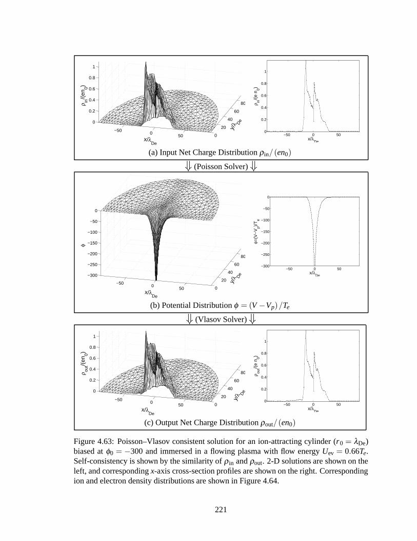
−500
50 0
20
40
60
80
0
0.2
0.4
0.6
0.8
1
ρ in/(
en0)
x/λDe
y/λ D
e
−50 0 500
0.2
0.4
0.6
0.8
1
x/λDe
ρ in/(
e n 0)
(a) Input Net Charge Distribution ρin/(en0)
⇓ (Poisson Solver)⇓
−500
50 0
20
40
60
80
−300
−250
−200
−150
−100
−50
0
φ
x/λDe
y/λ D
e −50 0 50
−300
−250
−200
−150
−100
−50
0
x/λDe
φ=(V
−V
p)/T
e
(b) Potential Distribution φ = (V −Vp)/Te
⇓ (Vlasov Solver)⇓
−500
50 0
20
40
60
80
0
0.2
0.4
0.6
0.8
1
ρ out/(
en0)
x/λDe
y/λ D
e
−50 0 500
0.2
0.4
0.6
0.8
1
x/λDe
ρ out/(
e n 0)
(c) Output Net Charge Distribution ρout/(en0)
Figure 4.63: Poisson–Vlasov consistent solution for an ion-attracting cylinder (r0 = λDe)biased at φ0 = −300 and immersed in a flowing plasma with flow energy Uev = 0.66Te.Self-consistency is shown by the similarity of ρin and ρout. 2-D solutions are shown on theleft, and corresponding x-axis cross-section profiles are shown on the right. Correspondingion and electron density distributions are shown in Figure 4.64.
221
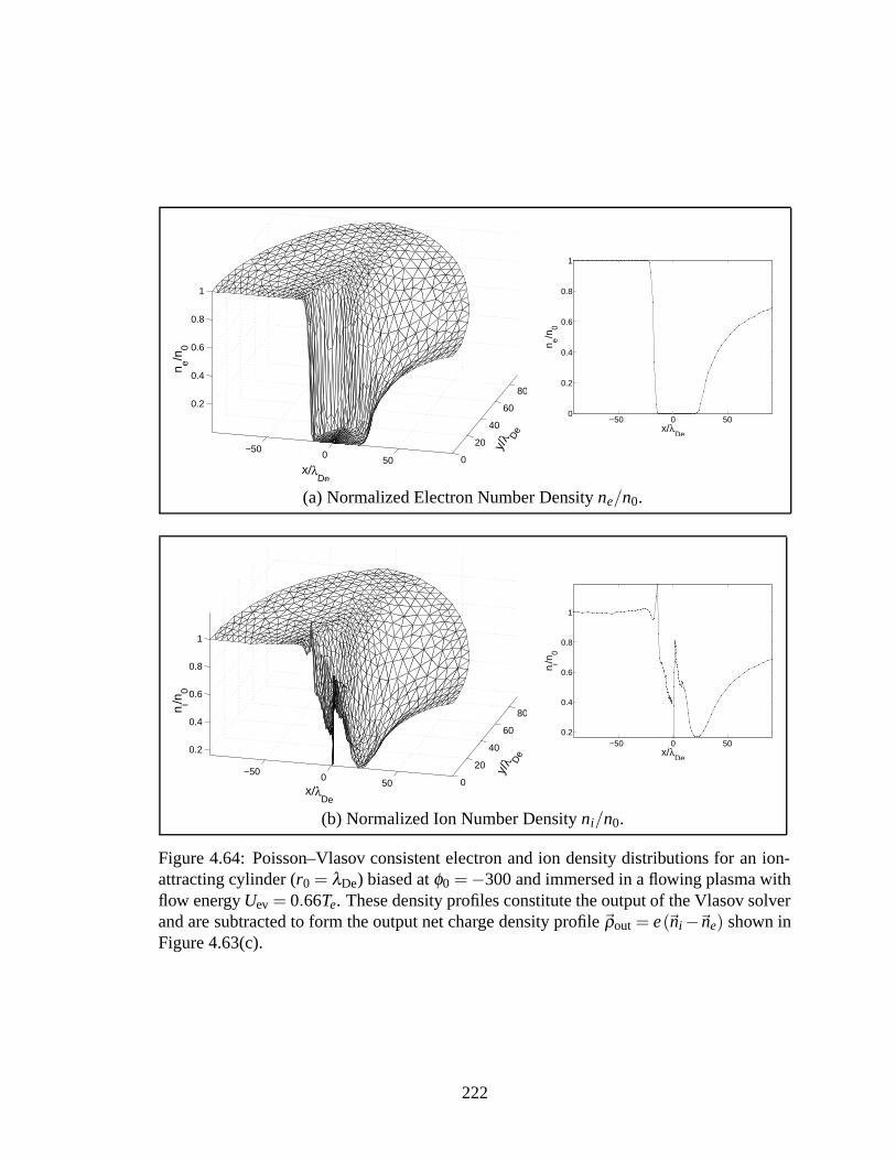
−500
50 0
20
40
60
800.2
0.4
0.6
0.8
1
n e/n0
x/λDe
y/λ D
e −50 0 50
0
0.2
0.4
0.6
0.8
1
x/λDe
n e/n0
(a) Normalized Electron Number Density ne/n0.
−500
50 0
20
40
60
80
0.2
0.4
0.6
0.8
1
n i/n0
x/λDe
y/λ D
e −50 0 50
0.2
0.4
0.6
0.8
1
x/λDe
n i/n0
(b) Normalized Ion Number Density ni/n0.
Figure 4.64: Poisson–Vlasov consistent electron and ion density distributions for an ion-attracting cylinder (r0 = λDe) biased at φ0 =−300 and immersed in a flowing plasma withflow energy Uev = 0.66Te. These density profiles constitute the output of the Vlasov solverand are subtracted to form the output net charge density profile �ρout = e(�ni−�ne) shown inFigure 4.63(c).
222

−200
−100
−50
−20
−10
φ0=−5
−300
−50 −40 −30 −20 −10 0 10 20 30 40 50−300
−250
−200
−150
−100
−50
0
Potential Profile on X axis (r0=λ
De,U
ev=0.66 T
e)
x/λDe
Nor
mal
ized
Pot
entia
l V/T
e
Figure 4.65: Set of curves of the axial potential profiles corresponding to various biaspotentials for a one-Debye-length-radius round cylinder immersed in a flowing plasma withflow energy Uev = 0.66Te. The profiles are taken along the axis of the flow.
4.5.4.3 Plasma Flow Effects on Sheath Structure and Dimensions
One wonders what the overall effect of this asymmetric distribution will be on the
sheath structure and size, since the main parameter of interest for charge precipitation ap-
plications is the overall sheath size. Using the concept of effective sheath area As which we
defined in Section 4.3.5, we now proceed to a similar analysis as that which was performed
in Section 4.3.6 for the two-cylinder configuration.
Figure 4.67 depicts the variation of the effective sheath area ratio, defined by (4.27), as a
function of bias potential, for a round cylinder with a radius r0= λDe immersed in a flowing
plasma with flow energy Uev = 0.66Te. The plot suggests that the effective sheath ratio
stabilizes near half (50%) of the stationary effective sheath area, and there is no indication
that this ratio would increase back to higher levels at larger bias potentials. However,
simulations should be performed at higher bias potentials to confirm the observed trend. It
223
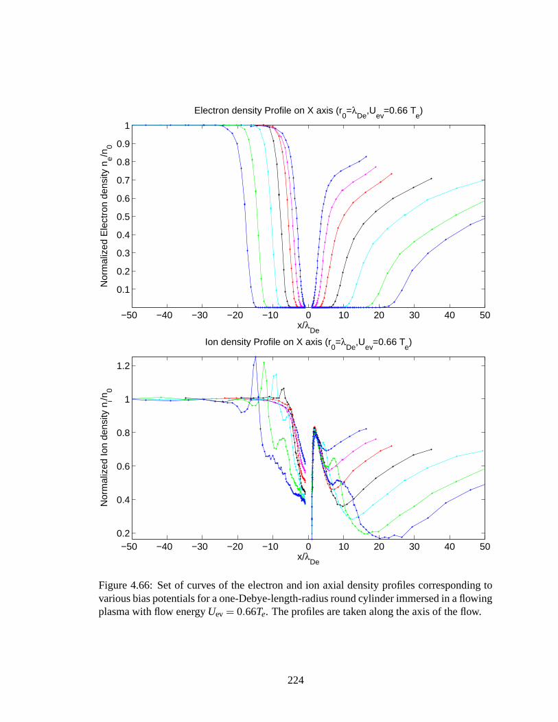
φ0=−5
−10 −20
−50
−100
−200 −300
−50 −40 −30 −20 −10 0 10 20 30 40 50
0.1
0.2
0.3
0.4
0.5
0.6
0.7
0.8
0.9
1
Electron density Profile on X axis (r0=λ
De,U
ev=0.66 T
e)
x/λDe
Nor
mal
ized
Ele
ctro
n de
nsity
ne/n
0
φ0=−5
−10 −20
−50 −100
−200
−300
−50 −40 −30 −20 −10 0 10 20 30 40 500.2
0.4
0.6
0.8
1
1.2
Ion density Profile on X axis (r0=λ
De,U
ev=0.66 T
e)
x/λDe
Nor
mal
ized
Ion
dens
ity n
i/n0
Figure 4.66: Set of curves of the electron and ion axial density profiles corresponding tovarious bias potentials for a one-Debye-length-radius round cylinder immersed in a flowingplasma with flow energy Uev = 0.66Te. The profiles are taken along the axis of the flow.
224
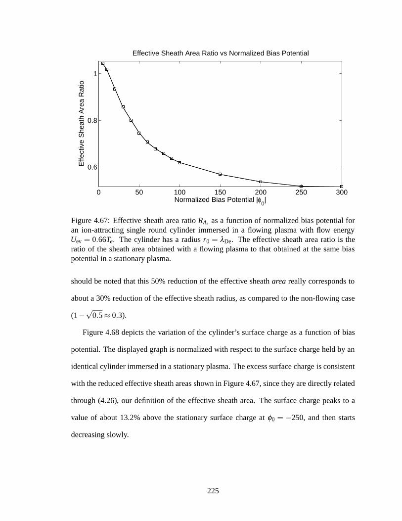
0 50 100 150 200 250 300
0.6
0.8
1
Effective Sheath Area Ratio vs Normalized Bias Potential
Normalized Bias Potential |φ0|
Effe
ctiv
e S
heat
h A
rea
Rat
io
Figure 4.67: Effective sheath area ratio RAs as a function of normalized bias potential foran ion-attracting single round cylinder immersed in a flowing plasma with flow energyUev = 0.66Te. The cylinder has a radius r0 = λDe. The effective sheath area ratio is theratio of the sheath area obtained with a flowing plasma to that obtained at the same biaspotential in a stationary plasma.
should be noted that this 50% reduction of the effective sheath area really corresponds to
about a 30% reduction of the effective sheath radius, as compared to the non-flowing case
(1−√
0.5≈ 0.3).
Figure 4.68 depicts the variation of the cylinder’s surface charge as a function of bias
potential. The displayed graph is normalized with respect to the surface charge held by an
identical cylinder immersed in a stationary plasma. The excess surface charge is consistent
with the reduced effective sheath areas shown in Figure 4.67, since they are directly related
through (4.26), our definition of the effective sheath area. The surface charge peaks to a
value of about 13.2% above the stationary surface charge at φ0 = −250, and then starts
decreasing slowly.
225

0 50 100 150 200 250 300
1
1.02
1.04
1.06
1.08
1.1
1.12
1.14
Surface Charge Ratio vs Normalized Bias Potential
Normalized Bias Potential |φ0|
Sur
face
Cha
rge
Rat
io
Figure 4.68: Ratio of surface charge to the “stationary” surface charge as a function ofnormalized bias potential, for an ion-attracting single round cylinder immersed in a flowingplasma with flow energy Uev = 0.66Te. The cylinder has a radius r0 = λDe.
4.5.4.4 Plasma Flow Effect on Ion Current Collection
Figure 4.69 depicts the variation of the ion current ratio as a function of normalized bias
potential φ0. This “current ratio” is simply the ratio of the current collected with flow, Iflow,
to the current collected without flow, Inoflow, for a given bias potential. The ratio is seen
to drop below 0.7 and possibly follows an asymptotic behavior with an asymptote of about
0.65. This is consistent with the very low ionic density observed in Section 4.5.4.2 on the
wake side of the cylinder’s surface. This current reduction is actually a unique feature of
low flow energies, since as the lower graph in Figure 4.49 shows, a current reduction only
occurs for a limited range of flow speeds, beyond which current enhancement becomes the
norm.
For the particle precipitation application, the reduction of the sheath area observed in
Section 4.5.4.3 will therefore be somewhat compensated by a reduction of the collected ion
current. This implies that, for a given power budget, the bias potential could be set higher
226
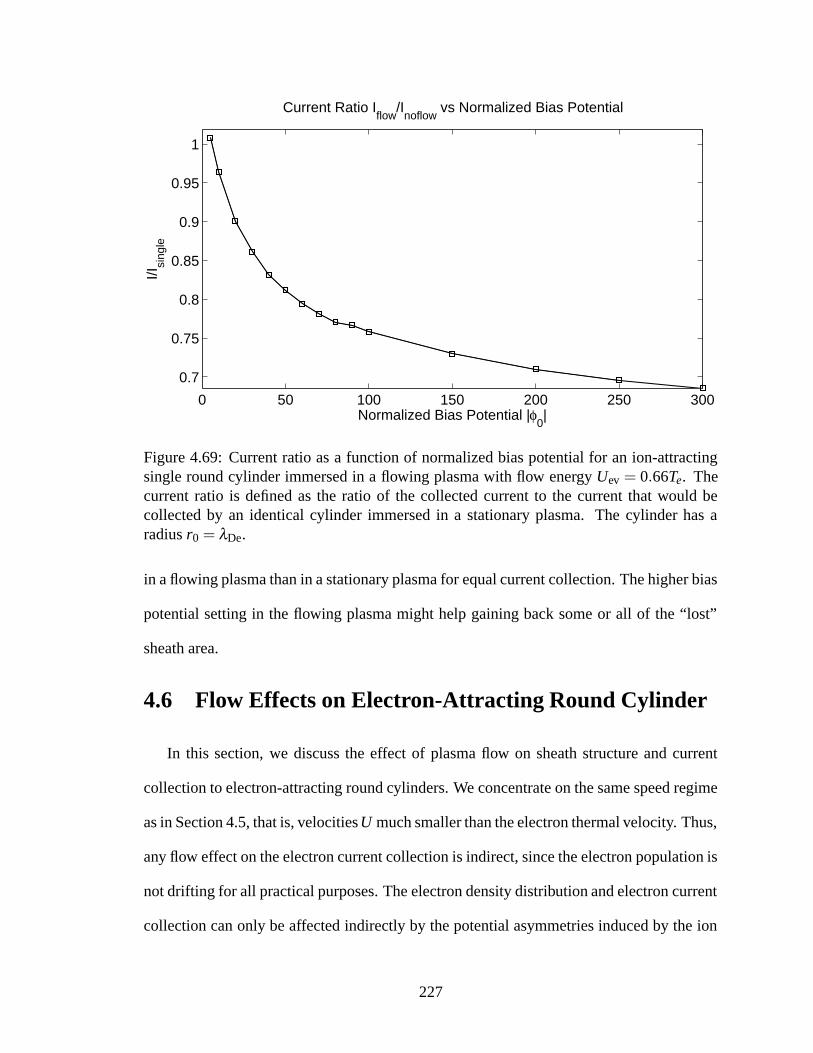
0 50 100 150 200 250 300
0.7
0.75
0.8
0.85
0.9
0.95
1
Current Ratio Iflow
/Inoflow
vs Normalized Bias Potential
Normalized Bias Potential |φ0|
I/Isi
ngle
Figure 4.69: Current ratio as a function of normalized bias potential for an ion-attractingsingle round cylinder immersed in a flowing plasma with flow energy Uev = 0.66Te. Thecurrent ratio is defined as the ratio of the collected current to the current that would becollected by an identical cylinder immersed in a stationary plasma. The cylinder has aradius r0 = λDe.
in a flowing plasma than in a stationary plasma for equal current collection. The higher bias
potential setting in the flowing plasma might help gaining back some or all of the “lost”
sheath area.
4.6 Flow Effects on Electron-Attracting Round Cylinder
In this section, we discuss the effect of plasma flow on sheath structure and current
collection to electron-attracting round cylinders. We concentrate on the same speed regime
as in Section 4.5, that is, velocities U much smaller than the electron thermal velocity. Thus,
any flow effect on the electron current collection is indirect, since the electron population is
not drifting for all practical purposes. The electron density distribution and electron current
collection can only be affected indirectly by the potential asymmetries induced by the ion
227

flow.
In the following analysis, we will only consider a single value of the normalized bias
potential, φ0 = 20, and study the effect of flow speed on the sheath structure and current
collection. We will then compare the simulated electron current collection to that observed
experimentally in Chapter 3.
4.6.1 Potential and Density Profiles
In Figures 4.70 through 4.77, we show some examples of plasma profiles pertaining to
an electron-attracting round cylinder biased at φ0 = 20 for various flow energies spanning
from Uev = 0.2Te to Uev = 1.5Te. The self-consistency of the results is illustrated by the
fact that the input and output net charge density distributions �ρin and �ρout are very close to
one another.
Although the potential profile corresponding to the lowest flow setting of Uev = 0.2Te
(shown in Figure 4.70) only shows what appears to be a minor asymmetry, a significant
effect is seen on both density profiles, but especially on the electron density profile (the
attracted species). The latter shows, on the ram side of the cylinder, a quasi-absence of
the usual density drop associated with the shadowing effect and angular momentum limi-
tations, and a deepening of the density drop on the wake side. The asymmetry allows more
electrons to penetrate closer to the cylinder on the ram side, while increasing the shadowing
effect of the cylinder on the wake side due to an increased focusing of the shadowed tra-
jectories. At Uev = 0.2Te, the plasma flow is not sufficiently energetic to prevent electrons
from reaching the wake-side surface of the cylinder, which is why a near-OML electron
density (just short of half the ambient density) is seen in Figure 4.71 for both the ram and
wake sides of the cylinder.
As the flow speed increases to higher values, several observations can be made:
228

−20 −10 0 10 20 0
5
10
15
20
−0.7
−0.6
−0.5
−0.4
−0.3
−0.2
−0.1
0ρ in
/(en
0)
xn=x/λ
De
y n=y
/λ De
−20 −10 0 10 20
−0.7
−0.6
−0.5
−0.4
−0.3
−0.2
−0.1
0
x/λDe
ρ in/(
e n 0)
(a) Input Net Charge Distribution ρin/(en0)
⇓ (Poisson Solver)⇓
−20 −10 0 10 20 0
5
10
15
20
0
5
10
15
20
φ=(V
−V
p)/T
e
xn=x/λ
De
y n=y
/λ De
−20 −10 0 10 200
5
10
15
20
x/λDe
φ=(V
−V
p)/T
e
(b) Potential Distribution φ = (V −Vp)/Te
⇓ (Vlasov Solver)⇓
−20 −10 0 10 20 0
5
10
15
20
−0.7
−0.6
−0.5
−0.4
−0.3
−0.2
−0.1
0
ρ out/(
en0)
xn=x/λ
De
y n=y
/λ De
−20 −10 0 10 20
−0.7
−0.6
−0.5
−0.4
−0.3
−0.2
−0.1
0
x/λDe
ρ out/(
e n 0)
(c) Output Net Charge Distribution ρout/(en0)
Figure 4.70: Poisson–Vlasov consistent solution for an electron-attracting cylinder (r0 =λDe) biased at φ0 = 20 and immersed in a flowing plasma with flow energy Uev = 0.2 Te.Self-consistency is shown by the similarity of ρin and ρout. 2-D solutions are shown onthe left, and corresponding x-axis cross-section profiles are shown on the right. Ion andElectron density dist. are shown in Figure 4.71.
229
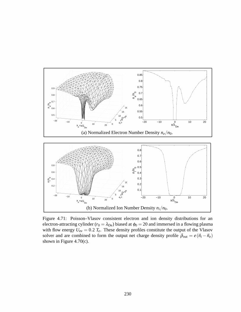
−20 −10 0 10 20 0
5
10
15
20
0.5
0.6
0.7
0.8
0.9
n e/n0
xn=x/λ
De
y n=y
/λ De
−20 −10 0 10 20
0.5
0.55
0.6
0.65
0.7
0.75
0.8
0.85
x/λDe
n e/n0
(a) Normalized Electron Number Density ne/n0.
−20 −10 0 10 20 0
5
10
15
20
0.2
0.4
0.6
0.8
n i/n0
xn=x/λ
De
y n=y
/λ De
−20 −10 0 10 20
0.1
0.2
0.3
0.4
0.5
0.6
0.7
0.8
x/λDe
n i/n0
(b) Normalized Ion Number Density ni/n0.
Figure 4.71: Poisson–Vlasov consistent electron and ion density distributions for anelectron-attracting cylinder (r0 = λDe) biased at φ0 = 20 and immersed in a flowing plasmawith flow energy Uev = 0.2 Te. These density profiles constitute the output of the Vlasovsolver and are combined to form the output net charge density profile �ρout = e(�ni−�ne)shown in Figure 4.70(c).
230

−20 −10 0 10 20 0
5
10
15
20
−0.7
−0.6
−0.5
−0.4
−0.3
−0.2
−0.1
0ρ in
/(en
0)
xn=x/λ
De
y n=y
/λ De
−20 −10 0 10 20
−0.7
−0.6
−0.5
−0.4
−0.3
−0.2
−0.1
0
x/λDe
ρ in/(
e n 0)
(a) Input Net Charge Distribution ρin/(en0)
⇓ (Poisson Solver)⇓
−20 −10 0 10 20 0
5
10
15
20
0
5
10
15
20
φ=(V
−V
p)/T
e
xn=x/λ
De
y n=y
/λ De
−20 −10 0 10 200
5
10
15
x/λDe
φ=(V
−V
p)/T
e
(b) Potential Distribution φ = (V −Vp)/Te
⇓ (Vlasov Solver)⇓
−20 −10 0 10 20 0
5
10
15
20
−0.7
−0.6
−0.5
−0.4
−0.3
−0.2
−0.1
0
ρ out/(
en0)
xn=x/λ
De
y n=y
/λ De
−20 −10 0 10 20
−0.7
−0.6
−0.5
−0.4
−0.3
−0.2
−0.1
0
x/λDe
ρ out/(
e n 0)
(c) Output Net Charge Distribution ρout/(en0)
Figure 4.72: Poisson–Vlasov consistent solution for an electron-attracting cylinder (r0 =λDe) biased at φ0 = 20 and immersed in a flowing plasma with flow energy Uev = 0.5 Te.Self-consistency is shown by the similarity of ρin and ρout. 2-D solutions are shown onthe left, and corresponding x-axis cross-section profiles are shown on the right. Ion andElectron density dist. are shown in Figure 4.73.
231

−20 −10 0 10 20 0
5
10
15
20
0.5
0.6
0.7
0.8
0.9
n e/n0
xn=x/λ
De
y n=y
/λ De
−20 −10 0 10 20
0.45
0.5
0.55
0.6
0.65
0.7
0.75
0.8
0.85
x/λDe
n e/n0
(a) Normalized Electron Number Density ne/n0.
−20 −10 0 10 20 0
5
10
15
200.2
0.4
0.6
0.8
n i/n0
xn=x/λ
De
y n=y
/λ De
−20 −10 0 10 20
0.1
0.2
0.3
0.4
0.5
0.6
0.7
0.8
x/λDe
n i/n0
(b) Normalized Ion Number Density ni/n0.
Figure 4.73: Poisson–Vlasov consistent electron and ion density distributions for anelectron-attracting cylinder (r0 = λDe) biased at φ0 = 20 and immersed in a flowing plasmawith flow energy Uev = 0.5 Te. These density profiles constitute the output of the Vlasovsolver and are combined to form the output net charge density profile �ρout = e(�ni−�ne)shown in Figure 4.72(c).
232

−20 −10 0 10 20 0
10
20
−0.7
−0.6
−0.5
−0.4
−0.3
−0.2
−0.1
0
y n=y
/λ De
xn=x/λ
De
ρ in/(
en0)
−20 −10 0 10 20−0.7
−0.6
−0.5
−0.4
−0.3
−0.2
−0.1
0
x/λDe
ρ in/(
e n 0)
(a) Input Net Charge Distribution ρin/(en0)
⇓ (Poisson Solver)⇓
−20 −10 0 10 20 0
10
20
0
5
10
15
20y n
=y/λ D
e
xn=x/λ
De
φ=(V
−V
p)/T
e
−20 −10 0 10 20
0
5
10
15
20
x/λDe
φ=(V
−V
p)/T
e
(b) Potential Distribution φ = (V −Vp)/Te
⇓ (Vlasov Solver)⇓
−20 −10 0 10 20 0
10
20
−0.7
−0.6
−0.5
−0.4
−0.3
−0.2
−0.1
0
ρ out/(
en0)
xn=x/λ
De
y n=y
/λ De
−20 −10 0 10 20−0.7
−0.6
−0.5
−0.4
−0.3
−0.2
−0.1
0
x/λDe
ρ out/(
e n 0)
(c) Output Net Charge Distribution ρout/(en0)
Figure 4.74: Poisson–Vlasov consistent solution for an electron-attracting cylinder (r0 =λDe) biased at φ0 = 20 and immersed in a flowing plasma with flow energy Uev = Te. Self-consistency is shown by the similarity of ρin and ρout. 2-D solutions are shown on the left,and corresponding x-axis cross-section profiles are shown on the right. Ion and Electrondensity dist. are shown in Figure 4.75.
233

−20 −10 0 10 20 0
10
20
0.4
0.5
0.6
0.7
0.8
0.9
n e/n0
xn=x/λ
De
y n=y
/λ De
−20 −10 0 10 20
0.4
0.6
0.8
x/λDe
n e/n0
(a) Normalized Electron Number Density ne/n0.
−20 −10 0 10 20 0
10
200.2
0.4
0.6
0.8
n i/n0
xn=x/λ
De
y n=y
/λ De
−20 −10 0 10 20
0.1
0.2
0.3
0.4
0.5
0.6
0.7
0.8
x/λDe
n i/n0
(b) Normalized Ion Number Density ni/n0.
Figure 4.75: Poisson–Vlasov consistent electron and ion density distributions for anelectron-attracting cylinder (r0 = λDe) biased at φ0 = 20 and immersed in a flowing plasmawith flow energy Uev= Te. These density profiles constitute the output of the Vlasov solverand are combined to form the output net charge density profile �ρout = e(�ni−�ne) shown inFigure 4.74(c).
234

−20 −10 0 10 20 0
10
20
−0.7
−0.6
−0.5
−0.4
−0.3
−0.2
−0.1
0ρ in
/(en
0)
xn=x/λ
De
y n=y
/λ De
−20 −10 0 10 20−0.7
−0.6
−0.5
−0.4
−0.3
−0.2
−0.1
0
x/λDe
ρ in/(
e n 0)
(a) Input Net Charge Distribution ρin/(en0)
⇓ (Poisson Solver)⇓
−20 −10 0 10 20 0
10
20
0
5
10
15
20
φ=(V
−V
p)/T
e
xn=x/λ
De
y n=y
/λ De
−20 −10 0 10 20
0
5
10
15
20
x/λDe
φ=(V
−V
p)/T
e
(b) Potential Distribution φ = (V −Vp)/Te
⇓ (Vlasov Solver)⇓
−20 −10 0 10 20 0
10
20
−0.7
−0.6
−0.5
−0.4
−0.3
−0.2
−0.1
0
ρ out/(
en0)
xn=x/λ
De
y n=y
/λ De
−20 −10 0 10 20−0.7
−0.6
−0.5
−0.4
−0.3
−0.2
−0.1
0
x/λDe
ρ out/(
e n 0)
(c) Output Net Charge Distribution ρout/(en0)
Figure 4.76: Poisson–Vlasov consistent solution for an electron-attracting cylinder (r0 =λDe) biased at φ0 = 20 and immersed in a flowing plasma with flow energy Uev = 1.5 Te.Self-consistency is shown by the similarity of ρin and ρout. 2-D solutions are shown onthe left, and corresponding x-axis cross-section profiles are shown on the right. Ion andElectron density dist. are shown in Figure 4.77.
235

−20 −10 0 10 20 0
10
20
0.3
0.4
0.5
0.6
0.7
0.8
0.9
y n=y
/λ De
x
n=x/λ
De
n e/n0
−20 −10 0 10 20
0.3
0.4
0.5
0.6
0.7
0.8
x/λDe
n e/n0
(a) Normalized Electron Number Density ne/n0.
−20 −10 0 10 20 0
10
200.2
0.4
0.6
0.8
y n=y
/λ De
xn=x/λ
De
n i/n0
−20 −10 0 10 20
0.1
0.2
0.3
0.4
0.5
0.6
0.7
0.8
x/λDe
n i/n0
(b) Normalized Ion Number Density ni/n0.
Figure 4.77: Poisson–Vlasov consistent electron and ion density distributions for anelectron-attracting cylinder (r0 = λDe) biased at φ0 = 20 and immersed in a flowing plasmawith flow energy Uev = 1.5 Te. These density profiles constitute the output of the Vlasovsolver and are combined to form the output net charge density profile �ρout = e(�ni−�ne)shown in Figure 4.76(c).
236

• A potential depression (below 0 V) appears on the wake side of the cylinder, which
gets deeper with increasing flow energy. This acts as a potential barrier which pre-
vents some electrons coming from the right from reaching close to the cylinder.
• The ion number density plateaus longer on the ram side, due to its increased inertia
associated with the increasing flow energy.
• Since quasi-neutrality must be satisfied at sufficiently large distances from the cylin-
der’s surface, the electron number density also plateaus longer on the ram side, before
dropping to half the ambient density on the ram-side of the cylinder’s surface. The
mechanism that allows this is the focusing of leftward-directed electrons onto the
ram-side potential “bump”.
• The bottom level of the wake-side dip in the electron number density goes deeper
as the flow energy increases, which is due to the repelling effect of the wake-side
potential depression, preventing some electrons from approaching the cylinder from
the wake side.
• The wake-side surface electron density drops below the OML value to values below
half the ambient density. This effect does not occur as quickly as the decrease of
the previously described “wake-side dip level density” because it is countered by the
geometrical concentration of electron current.
4.6.2 Electron Current Collection
We now turn to the analysis of electron current collection in a flowing plasma. Fig-
ure 4.78 shows the dependence of electron current on flow energy. It can be seen that
the amount of collected electron current goes down with increasing flow energy. This can
be explained by the action of the previously described wake-side potential barrier which
237

0 0.2 0.4 0.6 0.8 1 1.2 1.4 1.6 1.80.82
0.84
0.86
0.88
0.9
0.92
0.94
0.96
0.98
Uev
/Te
I e/I oml
Electron Current Ratio Ie/I
oml vs Flow Energy
Figure 4.78: Collected Electron Current Ratio Ie/Ioml as a function of the normalized flowenergy Uev/Te (φ0 = 20, r0 = λDe).
blocks electrons with insufficient energy from accessing the vicinity of the cylinder from
the wake side. Since the potential barrier grows with increasing flow energy, the collected
current drops accordingly. On the ram side, the electron current is just below the OML
level (as can be inferred from the electron density profiles), so that the decrease in electron
current is wholly attributed to the growth of the wake-side potential barrier.
Now, as the reader may recall from Chapter 3, our experimental measurements have led
us to conclude that there is a significant enhancement of the electron current with respect to
the orbital motion limit, contrary to what our simulation results indicate here. Figure 3.8 (a)
indeed indicates strong enhancements of about 25% at φ0 = 20 and 40% at φ0 = 100 for
the reference cylinder’s collected electron current with respect to OML, when placed at
the closest position with respect to the plasma source, where a large fraction of the ion
population was determined to be high speed ions with an energy of about 25 eV, or 13.9Te.
The reduced enhancement seen at 160 cm, along with the absence of any enhancement
at 300 cm, re-enforce our confidence that the strong enhancement observed at 75 cm is
238
indeed a consequence of the plasma flow, as opposed to an artifact of the measurement
errors involved in the determination of the plasma density for example.
If we assume that the observed enhancement was real, then there must be some addi-
tional important physics not included in our kinetic model that could potentially explain it.
Let us first ask the question of how much electron collection is possible given the assump-
tions used in our kinetic model. Following are two key facts for this discussion:
1. the plasma is assumed collisionless, and therefore only collisionless trajectories con-
nect the electron velocity distribution at a given point (r,θ) in space with a normal-
ized potential φ = V−VpTe
to the background plasma (r→ ∞ and φ = 0);
2. the electron population has no drift component in the background plasma, for all
practical purposes, because the electron thermal velocity vthe is much larger than
the drift velocity U . The background electron population (the source) can therefore
be accurately represented by a pure Maxwellian distribution, as given by (2.4) with
U = 0.
Given the collisionless assumption and the fact that the electrons are a stationary species,
we conclude that, in our kinetic simulations, the electron density at any position within
the potential structure cannot exceed the ambient density n0, nor can the collected electron
current to a probe exceed the orbital motion limit, as we show in Chapter 1 in accordance
with a proof given by Laframboise [6].
We hereby propose a possible mechanism for the experimentally observed current en-
hancement. As was seen in the collisionless self-consistent potential structures shown in
Figures 4.70 through 4.76, the electric potential stabilizes to a relatively large value on the
ram-side edge of the computational domain, which is on the order of the beam energy Uev.
The potential must therefore slowly drop from this relatively large potential down to zero
239

(the plasma potential) over a very large distance, since the electric field appears to already
be very low at the outer boundary of the computational domain, as expected within the
pre-sheath zone. Out at some distance on the x axis in the ram direction, the electric field
will have dropped to such a low level that some collisional forces would start dominating
electron behavior, even though the local potential would still be at a non-negligible fraction
of the electron temperature. This is unlike the symmetric stationary problem, in which the
electric potential drops sufficiently fast that it reaches a very small fraction of Te before
the electric field has dropped to a sufficiently low level to allow some collisional forces to
dominate electron trajectories.
Mathematically speaking, we may compare the stationary and flowing cases by consid-
ering the asymptotic forms that the potential profile may take along the x axis, on the ram
side. In the stationary case, we have the asymptotic result φ = φ(Rref)Rref
r , for sufficiently
large values of r (see Section 2.3.2.1), where Rref is some reference radius. Our flowing
results seem to indicate a slower asymptotic drop of the potential on the ram side, i.e.,
φ = φ(Rref)(
Rrefr
)k, with k < 1. The normalized radial component of the electric field is
thus given by
Enr =−∂φ∂ r= φ(Rref) k
Rkref
rk+1 , (4.36)
which should be compared against the stationary electric field Enr,n f = φ(Rref)Rrefr2 . The
ratio of the “flowing” to “stationary” electric field expressions is given by
Enr(r)Enr,n f (r)
= k
(Rref
r
)k−1
< 1 for r > Rref and k < 1, (4.37)
which is clearly less than one as indicated, meaning that the radial component of the electric
field is weaker in the case of a flowing plasma.
In the collisional zone of the pre-sheath, where collision forces dominate electric field
forces, collisions gradually re-thermalize the electron population as it is accelerated down
240

the shallow potential well leading to the “collision-free” zone. In the process, the electron
temperature may rise by a small amount (i.e., collisional heating), but, more importantly,
there is an increased concentration of electrons on the ram-side of the collisional zone,
where the potential is positive (and electron-attracting). In other words, the incoming elec-
tron density at the outer boundary of the collision-free zone is larger than the ambient
density by an amount that depends primarily on the potential level on that boundary.21 A
fair approximation for this potential dependence is given by the Boltzmann approximation
ne≈ n0 exp(φ(r)), where n0 is the ambient plasma density, φ is the local normalized poten-
tial V/Te, and Te is the electron temperature, which we assume here has not changed, i.e.,
no significant heating has occurred. This collisional concentration process would thus lead
to an increased influx of electrons on the ram side of the sheath, and therefore an increased
collected current primarily on the ram side of the cylinder. If we estimate that the electron
flux to the ram side of the cylinder’s surface will increase by a factor corresponding to the
increased electron density at the outer edge of the collision-free zone, and further assume
that no electron collection takes place on the wake side at sufficiently large flow energies
due to the repelling effect of the wake-side potential depression, we may approximate the
enhanced electron current collection to a small cylinder by
Ie,flowing
Ie,stationary≈
12
exp(φcollision boundary
). (4.38)
According to this crude model, a 40% enhancement such as we have observed experi-
mentally for a bias potential φ0 = 100 and flow energy Uev = 25Te would correspond to
a normalized potential at the frontier between the collisional and collision-free zones of
φcollision boundary ≈ 1, that is, a potential on the order of electron temperature. Given the
ram-side pre-sheath potentials that were obtained in the simulation results shown in Fig-
21Note that we should more generally refer to a transitional zone between the collisional and collision-freezones rather than a well-defined boundary.
241

ures 4.70 through 4.77 which were applicable to low-speed flows from Uev = 0.1Te to
Uev = 1.5Te, a value of 1 for the ram-side pre-sheath potential does seem quite reasonable
for such a large flow energy as Uev = 13.9Te.
The implementation of a dual model which includes both collision-free and collisional
zones has previously been presented [77] and will require further refinement to accurately
predict the observed enhancements.
4.7 Outline of Simulation Resource Requirements
In this section we give a coarse overview of the costs, in terms of computer resources
and computing time, of the kinetic simulations that were performed as part of this work.
A detailed “operation count” has yet to be performed for both the 1-D cylindrical imple-
mentation (KiPS-1D solver) and full 2-D implementation (KiPS-2D solver), but we can
nonetheless provide an overall description of the resource costs involved.
4.7.1 1-D Cylindrical Implementation (KiPS-1D)
The KiPS-1D solver was implemented using Matlab™ and Fortran 90, as described
in Section 2.7. It runs on a single computer using a single processor, and uses a relatively
small amount of random-access memory (RAM), on the order of a few tens of megabytes,
well below the amount of available RAM on our Linux workstation, which has 4 GB of
RAM.
In order to illustrate the computing time requirements for KiPS-1D, we have run KiPS-
1D with r0 = λDe for several bias potential values from φ0 = −10 to φ0 = −12800. The
number of unknowns (samples) required to properly sample the problem increases with the
value of the bias potential. Figure 4.79 shows a plot of the number of iterations required for
convergence as a function of the number of unknowns, along with a plot of the CPU pro-
242

50 60 70 80 90 100 110 120 130 140 150
100
200
300
400
500
600
Num
ber
of It
erat
ions
Number of Iterations and CPU Time vs Number of Unknowns
50 60 70 80 90 100 110 120 130 140 150
20
40
60
80
100
120
140
CP
U ti
me
(s)
Number of unknowns
Figure 4.79: Number of iterations required for convergence and CPU time as a functionof the number of unknowns in KiPS-1D simulations involving a cylinder radius of r0 =λDe. The number of unknowns was modulated by changing the bias potential, since higherpotentials demand a larger number of grid samples.
cessing time required on our Linux workstation as a function of the number of unknowns.
One can see that the type of 1-D simulations that we have run as part of this project only
has modest computing time requirements, since the longest simulation on this graph took
less than 150 seconds.
Figure 4.80 shows that, when the number of unknowns is sufficiently low, the comput-
ing time scales roughly linearly with the number of iterations required for a given problem.
It appears that this behavior breaks down when the number of unknowns becomes larger,
which is likely a consequence of the increased time required to invert the linearized system
at each iteration.
243

0 100 200 300 400 500 600 7000
50
100
150
Number of iterations
CP
U ti
me(
s)
CPU Time vs Number of Iterations
Figure 4.80: CPU time as a function of the number of iterations required for convergencein KiPS-1D simulations involving a cylinder of radius r0 = λDe. The number of unknownswas modulated by changing the bias potential, since higher potentials demand a largernumber of grid samples.
4.7.2 2-D Cylindrical Implementation (KiPS-2D)
As was discussed in Section 2.7, the KiPS-2D solver is much more computationally
demanding. As the reader may recall from Section 2.7, the Poisson solver and Tikhonov-
regularized Newton iterative processes run on a single Linux workstation (2.4 GHz dual-
Xeon), while the Vlasov solver uses a collection of about 150 slave nodes running on a
dynamically-configured pool of Sun Blade™ 1000/1500 workstations in order to compute
the plasma density samples.
4.7.2.1 Processing Time
Although a detailed, careful analysis of the computing time requirements has not been
performed for KiPS-2D, we present in Figure 4.81 some timing data pertaining to the simu-
244

0 50 100 150 200 2500
20
40
60
80
100
120
|φ0|
CP
U ti
me
(hou
rs)
CPU time vs magnitude of bias potential φ0
Figure 4.81: Simulation time required as a function of the magnitude of the normalizedbias φ0, for the KiPS-2D simulations shown in Section 4.5.4, with r0 = λDe, Uev = 0.66Te,and one mesh refinement.
lation results shown in Section 4.5.4. Bare in mind that at least two other KiPS-2D simula-
tions were running simultaneously, competing for resources. Thus, the actual time spent for
these simulations would correspond to about one third of the values shown in Figure 4.81
or even less.
Generally speaking, the primary parts of the algorithm that contribute to the computing
time in KiPS-2D are the following (not necessarily in that order):
1. the Vlasov solver, which uses all 150 slave workstations to compute the density sam-
ples based on several thousand particle trajectories;
2. building the Poisson-Vlasov Jacobian matrix, as described by equation (2.115);
3. performing the Tikhonov regularization, which includes the selection of the regular-
245

ization parameter λ in (2.133).
A future thorough assessment of the computing requirements should include separate tim-
ings for each of those three major computational hurdles.
For the time being, we have been able to determine that the computational bottleneck
for KiPS-2D is different depending on the regime of operation. When the number of mesh
nodes is relatively small (i.e. 500 or less), the bulk of the time is spent in the Vlasov solver
(step 1), while steps 2 and 3 amount to a small fraction of the computing time; this is the
most efficient mode of operation. On the other hand, when the number of mesh nodes
becomes somewhat larger (1000 and above), the matrix manipulations involved in steps
2 and 3 now require the most computing time. The shift between these two regimes is
apparent in Figure 4.81, and seems to occur around a bias potential |φ0| = 100. The larger
bias potential values require more mesh refinement near the cylinder and therefore cause
a dramatic surge in the number of mesh nodes. For example, at |φ0| = 250 about 1800
mesh nodes are required, which implies the manipulation of matrices with dimensions of
1800×1800.
Thus, in its current state the 2-D solver is optimal for use at moderate bias voltages.
Future modifications should seek to minimize the bottleneck associated with high mesh
density in the vicinity of biased conductors. This could be done by using alternate rep-
resentations for the Poisson solver, over small areas near high-voltage conductors, which
are not based on a full discretization, but instead only discretize the perimeters surround-
ing those high-field areas. Such an approach would assume a negligible effect of the local
space charge in high-field areas near high-voltage conductors.
Another, rather simple improvement could be done to reduce the computing time in-
volved in step 2 above. The present implementation uses full matrices for JV when comput-
ing the Poisson-Vlasov Jacobian matrix JPV , which results in a pure matrix-matrix product
246
involving full matrices. However, as is explained in Appendix E, the approximation used
for the Vlasov Jacobian JV is merely a diagonal matrix. One could take advantage of this
fact in order to significantly speed up the matrix-matrix product involved in computing the
Poisson-Vlasov Jacobian matrix.
4.7.2.2 Random-Access Memory Requirements
The RAM requirement on slave nodes is very reasonable, typically on the order of ten
to a few tens of megabytes, and therefore does not constitute a bottleneck. On the master
workstation, RAM requirements can sometimes reach as high as 2 gigabytes, when building
very large matrices in problems involving high voltages probes, as described above. This
requirement should be relaxed significantly when the optimizations discussed above are
implemented. However, should the simulation of problems involving tens of thousands
of mesh nodes be required, one would have to consider moving to a 64-bit computing
platform, in order to reach beyond the memory addressing limit of 4 gigabytes 22 imposed
by 32-bit platforms such as the one that was used for this thesis.
22The practical limit is 3 gigabytes on a properly configured Linux kernel due to the operating systemoverhead.
247

CHAPTER 5
Conclusions and Recommendations for Future Research
Designing bare electrodynamic tethers for propellantless space propulsion or radiation
belt remediation will demand a detailed understanding of the impact of tether geometry
and ionospheric flow on plasma sheath structure and current collection. Geometries are
being sought that improve structural merits and survivability from collisions with microm-
eteroids, while optimizing sheath structure and current collection. Previous research on
sheath structure and current collection has only addressed low-voltage regimes and simple
round cylinders as collectors, whether it be in stationary or flowing plasmas.
5.1 Summary and Conclusions of Research
This research has sought to fill the gaps in the existing literature by investigating,
through both simulation and experimentation, the sheath structure physics and current col-
lection properties of cylindrical collectors with various cross-sectional geometries in sta-
tionary and flowing plasmas.
5.1.1 Self-Consistent Steady-State Kinetic Model
Because no suitable existing model could adequately support the structures and regimes
of interest, a novel computational model was devised to address the problems under con-
sideration. Using kinetic theory, a steady-state kinetic computational model was developed
248

which allows for the self-consistent modeling of collisionless, unmagnetized two-species
plasmas in a vast region surrounding an arbitrarily-shaped 2-D conductive object. This
model allows for both stationary and flowing plasmas. Following are some of its main
features:
• it can provide kinetic treatment for both species based on the dynamic sampling of
the velocity distribution function at a finite set of nodes;
• it provides a dynamic, adaptive, unstructured meshing strategy, allowing for the sup-
port of arbitrary 2-D geometries and the adequate resolution of plasma sheath fea-
tures, such as the narrow surge of the net charge density which exists near the sheath
edge in the case of high-voltage biases;
• it allows for the simulation of very large computational domains, based on tailoring
the variable grid size to efficiently accommodate potential and density variations;
• it uses a new approach, called the Progressive Tikhonov-Regularized Newton Method,
to efficiently minimize the Poisson–Vlasov residual in order to approximate the fixed
point of the Poisson–Vlasov operator. This approach is robust to numerical instabili-
ties and quadrature noise and has successfully been used to solve a wide class of 2-D
problems without the need for empirical adjustments;
• it includes a coarse-grained parallel implementation for its Vlasov solver, allowing it
to run on MPMD (Multiple Processors, Multiple Data) parallel architectures.
Based on this model, two solvers were developed: a 1-D cylindrical model, implemented
in a solver called KiPS-1D, and a full 2-D model, implemented in KiPS-2D. The relative
computational simplicity of the 1-D cylindrical model has allowed it to be used exten-
sively to develop a basic set of sheath profiles for high-voltage circular cylinders, after an
249

initial validation was performed based on the available literature that covers low bias po-
tential regimes. This also provided a reference for the validation of the more complex 2-D
solver, in addition to the available literature. Several asymmetric problems were simulated
in KiPS-2D, allowing for the characterization of the two-cylinder and solid tape config-
urations, as well as an assessment of flow effects on ion- and electron-attracting round
cylinders.
5.1.2 Experimental Investigation of Electron-Collecting Tether Sam-ples
An experimental investigation was performed which consisted of measuring electron
current collection to cylindrical, solid tape, and slotted tape electrodynamic-tether samples
in a mesosonic flowing xenon plasma. A Hall thruster was used to simulate a flowing
unmagnetized space plasma in a large 6-m × 9-m vacuum chamber. Solid tape samples
with effective widths spanning from 4.9 to 41.9 Debye lengths, and slotted tapes with
center-to-center line spacings spanning from 1.4 to 13.2 Debye lengths were tested. Several
conclusions were drawn from the analysis of the results:
• plasma flow leads to significant current enhancements over that predicted by the
orbital-motion-limited theory;
• the electron collection efficiency of solid tapes (on a per area basis) decreases as the
width of the tape is increased, consistent with our computer simulations;
• beyond a threshold bias potential close to the beam energy, solid and slotted tapes
both collect more current when oriented transverse to the flow;
• equivalent-width slotted tapes are more efficient electron collectors than solid tapes
on a per area basis;
250
• the data suggests that the electron collection efficiency of slotted tapes decreases
with increasing line spacing until a minimum efficiency is attained, beyond which
it is expected to increase monotonically up to the orbital-motion limit expected of
independent lines.
5.1.3 Important Simulation and Experimental Results
Kinetic simulations and experimental investigations have allowed several new results
to be obtained. We describe the major results in the following.
5.1.3.1 Ion-Attracting High-Voltage Single Cylinder in Stationary Plasma
Acceleration of attracted ions into the high-voltage sheath results in a significant deple-
tion of ions within a large portion of the sheath, primarily as a result of flux conservation.
This is the primary mechanism allowing for the creation of relatively large sheath radii,
as compared to what may have been expected from a uniform ion density assumption, for
example. An asymptotic equation relating the normalized bias potential φ0 and cylinder
radius r0 to the effective sheath radius rs was obtained in (4.19) and is repeated here:
2.554
(rs
λDe
)1.325
lnrs
r0=−φ0. (5.1)
5.1.3.2 Interference Effects of Parallel Cylinders
Interference effects between two parallel cylinders were shown to exist for spacings
upward of 20 times the single-cylinder sheath radius, and an optimal spacing equal to the
single-cylinder sheath radius was seen to maximize the overall sheath area to a value equal
to twice the independent single-cylinder effective sheath area (for one value of the bias
potential, φ0 = −320). In addition, for a spacing of half the single-cylinder sheath ra-
dius, current collection is reduced to a minimum of half of the current collected by two
independent cylinders. This is attributed to the existing set of unpopulated collisionless
251

paths connecting both cylinders which create voids in the incoming velocity distribution
at the cylinders’ surfaces, thereby reducing the collected current. This particular spacing
is thought to maximize the number of such unpopulated orbits bounded by the cylinders,
hence the minimal current collection.
5.1.3.3 Geometry Effects of the Solid Tape Cylinder
The capacitance-based equivalent circular radius of a solid tape biased at a normalized
bias potential φ0 = −320 was shown to be approximately equal to 0.29w, where w is the
tape width. This result was verified over a large range of tape widths spanning from 1 to
50 Debye lengths, and is slightly higher than a previous asymptotic result of 0.25w [11].
On a per-area basis, solid tapes have a reduced current collection capability as compared
to that of an equal-capacitance circular cylinder. The general character of the departure
of collected current from the orbital motion limit value has been shown to agree, within
experimental uncertainties, with experimental current measurements on solid tapes after
normalizing out flow enhancement effects using data from a reference cylinder.
5.1.3.4 Plasma Flow Effects on Ion-Attracting Cylinder
Flow effects on ion-attracting cylinders were investigated through kinetic simulations
using KiPS-2D. Results indicate that flow energies representing any significant fraction of
the plasma temperature are sufficient to cause significant sheath asymmetries, regardless
of the bias potential applied on the cylinder. In fact, asymmetries were seen to grow with
increasing applied bias potential. For a flow energy of 66% of the thermal energy of the
plasma, results indicate a reduction of the effective sheath radius by about 30% (the sheath
area was reduced by about 50%) at large bias potentials with respect to the stationary case.
The collected current was also reduced by about 30%, which translates into a 30% savings
in terms of power expenditure for a given bias voltage.
252

5.1.3.5 Plasma Flow Effects on Electron-Attracting Cylinder
Flow effects on electron-attracting cylinders were investigated through both kinetic sim-
ulations and experimental investigations. Kinetic simulations have shown strong sheath
asymmetries with flow energies on the order of the plasma temperature, along with a re-
duction of the collected electron current attributed to the buildup of a potential barrier for
electrons downstream of the cylinder. Our experimental results, however, have shown a
clear enhancement of electron current collection over the orbital-motion limit for a cylin-
der immersed in a flowing plasma.
Even though this measured current enhancement could not be predicted by our colli-
sionless simulations, the obtained simulated plasma profiles can help interpreting the cause
for the enhancement. The strong elongation of the pre-sheath potential structure, upstream
of the cylinder, points to the possible existence of a collisional zone for electrons with non
vanishing potentials, far upstream from the cylinder, where even weak collisional forces
would dominate electric field forces. The thermalizing effect of these weak collisions over
an extended range where the electric potential is still above zero would cause a concen-
tration of electrons with densities exceeding the ambient density upstream of the cylinder,
providing an increased influx of electrons on the ram side and thereby enhancing the col-
lected electron current. A somewhat analogous explanation of electron current enhance-
ment, which applies in the case of magnetized plasmas, is given by Cooke and Katz [81].
5.2 Recommendations for Future Research
Suggestions for future research can be categorized into 1) computational modeling and
2) experimental testing efforts.
253

5.2.1 Computational Modeling
Several problems of interest that have not yet been addressed should be simulated using
KiPS-2D:
1. The two-cylinder configuration should be generalized to allow for the simulation of
an arrangement of N cylinders, and to allow for the comparison of the merits of var-
ious arrangements with the goals of minimizing current collection and maximizing
sheath cross-section, two objectives pertaining to the particle precipitation applica-
tion.
2. Similarly, the slotted tape samples that were investigated experimentally as part of
this thesis should be simulated. This structure consists of a “fence” of four parallel
narrow tapes.
3. The study of ionospheric flow effects on ion-attracting cylinders should be extended
to include larger bias potentials, to verify the apparent asymptotic character of the
sheath area ratio.
Following are some key fundamental improvements to the kinetic model that should be
considered.
1. A more thorough study of the several “trapped” state criteria used for determining
whether a given trajectory is populated should be performed. A more general crite-
ria should be sought, if possible, that would be independent of the geometry under
consideration.
2. At large negative bias voltages it is possible that the ion bombardment to a tether
might cause secondary emission of electrons, causing an increase in the net collected
current. In order to study the possible impact of this effect, support should be added
254

in KiPS-1D and KiPS-2D for particle emission from conductive surfaces. A sepa-
rate, first-order initial analysis [82] has shown that, even though secondary electron
emission can contribute a significant amount of electron density near the cylinder’s
surface, its overall effect on the sheath structure should be negligible. The outward
acceleration of the repelled electrons is so important that, due to current conservation,
the secondary-electron density drops very quickly as we move away from the cylin-
der’s surface, to a degree such that the area over which significant electron density
can exist is very small and therefore cannot contribute significantly to space charge.
3. In an effort to better understand and characterize the flow-induced electron cur-
rent enhancement that was observed experimentally, support for weak thermaliz-
ing collisions based on a Krook model should be implemented or, alternatively, a
dynamically-defined collisional zone should be included based upon the local mag-
nitude of the electric field. Some work toward these tasks has already been initiated.
4. Support for periodic time variations could be added to the 1-D cylindrical implemen-
tation, in order to perform a self-consistent study of the effect of periodic excitations
of tether bias potentials. Such excitations may be used to affect the sheath struc-
ture and current collection properties, using the ponderomotive force for example, as
suggested by some analyses of the Oedipus C tethered payload experiment [83].
5. The computationally tractable range of the bias potential in the 2-D model could be
expanded by either one of the following two additions.
• Since the sheath solution is virtually independent of the density samples lo-
cated sufficiently close to a high-voltage conductive surface, one could signifi-
cantly reduce the computational cost of each iteration by excluding such nodes
from the Vlasov density calculations for all iterations but the last one (that is, if
255

knowledge of those densities is required at all). This procedure would alleviate
the steep increase in computational cost that results from the stringent require-
ments on mesh density near high-voltage surfaces, which are necessary for the
accurate tracking of trajectories transiting through those zones.
• The implementation of a second-order, piecewise quadratic approximation for
the potential and charge density distribution should be considered. It would en-
tail a re-formulation of the finite-element Poisson solver and a re-formulation
of the semi-analytical trajectory tracking process. This higher-order implemen-
tation would relax the meshing requirements for accurate trajectory tracking,
and thereby enable the solution of more complex problems.
6. Support for magnetic fields should be implemented. Depending on the field’s orien-
tation, this may however imply the need for the representation of three-dimensional
velocity space, which would come at a significant computational cost, but is nev-
ertheless foreseeable for the near future, assuming that the exponential growth of
computing power predicted by Moore’s law [84] continues to hold...
5.2.2 Experimental Testing
Continued experimental testing is necessary for the validation and refinement of the
analytical and computational models that will be used by designers. Following are sugges-
tions of future experimental tests that should be considered.
1. Although our experimental tests of slotted tape samples have allowed us to sample a
few effective gap spacings, they were not sufficient to adequately sample the current
ratio curve shown on Figure 4.39, for example. An ideal test setup to validate this
simulated data would consist of two thin cylinders (wires) which could be mechani-
cally moved to dynamically adjust the spacing between them, therefore providing a
256

means to adequately sample the relationship of current ratio as a function of spacing
using a dynamic selection of the spacing.
2. The sheath structure forming around one or several thin cylinders biased at a high
voltage is of primary interest for this research, and has only been investigated through
simulations as part of this thesis. The experimental validation of the sheath profiles
obtained in this thesis is instrumental for the future use of our kinetic model for
design purposes. A low-voltage bias probe could be used to sample the electron
density structure around such a high-voltage system in order to determine a measure
of the sheath structure and dimensions. This could then be used to validate the model.
One of the difficulties in devising such a system would be to minimize the perturbing
effect of the probe, but such a perturbation should not be critical in regard of the high
voltages involved in the sheaths under study.
3. The existence of the sheath asymmetries which have been identified through simula-
tions even with moderate flow energies (66% of thermal energy) should be assessed
experimentally. This could be done by measuring the electron density profile using
the low-voltage bias probe system described above, or, preferably, using a different
measurement method that would obtain a more direct measurement of the ion density.
257

APPENDICES
258

APPENDIX A
Nomenclature
The mksA (meter–kilogram–second-Ampere) units are used throughout this work, ra-
ther than cgs (centimeter–gram–second). The following is a listing of the major symbols
and variables used in this work, along with a brief description and the appropriate unit.
Nomenclature Description (Unit)
α Direction of particle velocity vector (rad)αc Angle between successive search directions (rad)αt
c Target value for αc (rad)β Step size of iterative resolution procedureαi Direction of particle velocity vector upon entry into the compu-
tational domain (rad)γ(n) Specified decay rate of the nth circular harmonic of the exterior
potentialΓe,i Electron/ion particle flux (s−1m−2)(∆V )max Absolute mesh error tolerance on electric potential∆x Center-to-center spacing between two cylinders (m)ε0 Vacuum permittivity (F/m)θvar Angular displacement (rad)κ Particle kinetic energy (eV)κrange Kinetic energy integration range (in terms of temperature T)λ Tikhonov regularization parameterλDe Debye length (m)µb Fraction of high-speed ionsΠ Energy functional of FEM-based Poisson solverΠ1 Energy functional associated with Laplace fieldsΠ2 Energy functional associated with exterior fieldsΠ3 Energy functional associated with space chargeΠdiscrete Numerical approximation of Πρ Net charge density (C/m3)
259

Nomenclature Description (Unit)
ρn Normalized net charge density�ρ Vector containing the net charge density samples at all mesh
nodes (C/m3)ρin(x,y) Input charge density distribution (input of Poisson functional)ρout(x,y) Output charge density distribution (output of Vlasov functional)�ρin Vector form of the input charge density distribution�ρout Vector form of the output charge density distributionσi ith singular value of the preconditioned system matrix A′
�σ Vector containing the singular values of the preconditioned sys-tem matrix A′
τrel Relative quadrature tolerance on number densitiesτabs,E Absolute tolerance on energy-quadrature errorτmesh,abs Absolute mesh error toleranceτmesh,n Absolute mesh error tolerance on the density distribution, rela-
tive to its total rangeτmesh,V Absolute mesh error tolerance on the electric potential distribu-
tion V (r,θ), relative to its total rangeτmesh,ρ Absolute mesh error tolerance on the net charge density distri-
bution ρ(r,θ), relative to its total rangeφ Normalized potentialφ0 Normalized bias potentialφcollision boundary Normalized potential at the frontier between collisional and
collision-free zonesa0i,ani,bni Quadrature coefficients used to approximate the Fourier series
coefficients of the potential profile on the outer boundary�a0,�an,�bn Vector form of the quadrature coefficients a0i,ani,bni
A0 Cylinder’s cross sectional area (m2)An Normalized area (in terms of λ 2
De)As Effective sheath area (m2)As,1 Single-cylinder effective sheath area (m2)As,virtual Virtual effective sheath area (m2)A∞ Surface of the domain exterior to the computational zoneA System matrixA′ Preconditioned system matrix�b Right-hand side of the linearized system of equationsb Transformed Poisson–Vlasov residualB Magnetic field intensity (Tesla)Dp Diagonal right preconditionere Constant (1.6×10⁻¹⁹ J/eV)E Transverse energy of a particle (J)Ekα ,kE = Ev(kα ,kE) Total energy of quadrature samples (eV)Emin Minimum transverse particle energy (J)
260

Nomenclature Description (Unit)
Enr Normalized radial component of the electric field under flowingconditions
Enr,n f Normalized radial component of the electric field for a non-flowing plasma
Er,Eθ Directional total energy components (eV)Ern nth azimuthal mode of the radial electric field on the outer
boundaryEv Total particle energy (eV)Ev,min,Ev,max Minimum and maximum total particle energies in quadrature
integration (eV)fE(E) 1-D total energy distributionf (vx,vy) 2-D velocity distributionfi(vxi,vyi) 2-D velocity distribution at the entry point on the outer bound-
ary of the computational domainfP Poisson functionalfPV Poisson–Vlasov functionalfV Vlasov functionalg(κ,α) 2-D directional kinetic energy distributiong(Ev,α) 2-D directional total energy distributionh Local grid size for 1-D modelhgoal Target local grid size for 1-D modelH Altitude (m)I Total collected current (A)Id Hall thruster discharge voltage (volts)Ie Collected electron current (A)Ii Collected ion current (A)Iim Hall thruster inner magnet current (A)Iindep Current collected on a single independent cylinder (A)Iom Hall thruster outer magnet current (A)In Normalized collected currentIoml Orbital motion limited current (A)Irefcyl Current collected to the reference cylinder (A)Itape Current collected to a thin tape (A)Itether Current flowing along tether (A)Ith Thermal current (A)Je,i Electron/ion current density (A/m2)Jth Thermal current density (A/m2)JP Jacobian matrix of the Poisson solverJV Jacobian matrix of the Vlasov SolverJPV Poisson–Vlasov Jacobian matrixK Stiffness matrix of the FEM-based Poisson formulationL Angular momentum (kg m2/s)Lr Special Definition given on page 52 (kg m2/s)
261

Nomenclature Description (Unit)
ma Hall thruster anode flow rate (sccm)mc Hall thruster cathode flow rate (sccm)me,i Electron/ion mass (kg)me,n,mi,n Normalized electron/ion massmod() Modulo functionMorb Maximum angular displacement (number of multiples of 2π)Mrosc Maximum number of radial oscillationsMsegcross Maximum number of intersections of any single edgen0 Background plasma number density (m−3)ne,i Electron/ion number density (m−3)nest Numerical estimate of number density (m−3)�ne,i Vector containing the Electron/ion number density samples at
all mesh nodes (m−3)N Number of mesh nodes (also the number of unknowns)NE(kα) Number of energy quadrature samples for the kth
α α-integralNmodes Number of azimuthal modes used to represent the outer bound-
ary potential profileNob Number of potential samples on the outer boundaryNr Number of mesh refinement stepsqe,i Electron/ion charge (C)qe,n,qi,n Normalized electron/ion chargeQ Loading matrix of the FEM-based Poisson formulationQ Linear surface charge (C/m)Qn Normalized surface chargeQn,1 Single-cylinder normalized surface charger0 Round cylinder radius (m)rG Gyroradius (m)rGL Larmor gyroradius (m)rM Radius of the outer boundary of the computational domain (m)rs Effective sheath radius (m)rs,1 Effective sheath radius of a single independent cylinder (m)RAs Effective sheath area ratioReq Equal-charge equivalent circular cylinder radius (m)Sd Ion speed ratioTe,i Ambient electron/ion temperature (eV)Te,n,Ti,n Normalized ion/electron temperatureTslow Temperature of a low-energy, non-flowing ion population (eV)U Plasma flow velocity (m/s)Uev Plasma flow energy (eV)vr,vθ Particle velocity components in cylindrical coordinates (m/s)vx,vy Particle velocity components in Cartesian coordinates (m/s)vxi,vyi Particle velocity components upon entry intro the computa-
tional domain (m/s)
262

Nomenclature Description (Unit)
vx f ,vy f Particle velocity components at the interrogation point withinthe computational domain (m/s)
vxn,vyn Normalized particle velocity componentsvx∞,vy∞ Particle velocity components in the background plasma, away
from the perturbation as r→ ∞ (m/s)V Potential (volts)V0 Bias potential (volts)�V Vector containing the potential samples at all mesh nodes (volts)�Vb Vector containing the potential samples on the outer boundary
(volts)Vavg,fit Average bias potential over which the ion saturation best fit is
performed as part of the Langmuir probe data analysisVc Hall thruster cathode voltage (volts)Vd Hall thruster discharge voltage (volts)Vedge Electric potential at the entry point of the particle on the outer
boundaryVemf Potential drop along an electrodynamic tether due to the net ef-
fect of motional electromotive force combined with an on-boardvoltage source (volts)
Vhtr Hall thruster Heather voltage (volts)Vp Plasma potential (volts)Vxn nth azimuthal mode of the electric potential on the outer bound-
ary (volts)�x Linearized system unknownsx Transformed system unknownsxi,yi Particle coordinates upon entry into the computational domain
(m)x f ,y f Coordinates of the interrogation point within the computational
domain (m)xn,yn Normalized coordinates (in terms of the Debye length)wk Quadrature weights, 1-D Vlasov solverwkα ,kE Quadrature weights, 2-D Vlasov solverz(t) = zAt2+ zBt+ zC Quadratic equation of the intersection of a sub-trajectory with a
mesh segment
263

APPENDIX B
Acronyms
Although most of the acronyms used are defined in the text, we have listed them here
for convenience.
Acronym Description
BAMG Bidimensional Anisotropic Mesh GeneratorCAEN Computer Aided Engineering NetworkCPU Central Processing UnitFEM Finite Element MethodHV High VoltageINRIA Institut National de Recherche en Informatique et en AutomatiqueISS International Space StationLIF Laser Induced FluorescenceLP Langmuir ProbeLVTF Large Vacuum Test FacilityNPACI National Partnership for Advanced Computational InfrastructurePEPL Plasmadynamics and Electric Propulsion LaboratoryRHS Right-Hand SideKiPS-1D Kinetic Plasma Solver, 1-DKiPS-2D Kinetic Plasma Solver, 2-DOML Orbital Motion LimitMFP Mean Free PathMPMD Multiple Processors, Multiple DataPIC Particle-In-CellPVM Parallel Virtual MachineSHV Super High Voltage
264
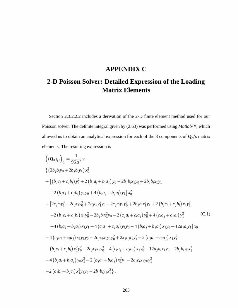
APPENDIX C
2-D Poisson Solver: Detailed Expression of the LoadingMatrix Elements
Section 2.3.2.2.2 includes a derivation of the 2-D finite element method used for our
Poisson solver. The definite integral given by (2.63) was performed using Matlab™, which
allowed us to obtain an analytical expression for each of the 3 components of Qn’s matrix
elements. The resulting expression is((Qn)i j
)ie=
196∆2×{(
2b jbiy0+2b jbiy1)
x30
+[(
b jci+ c jbi)
y21+2
(b jai+bia j
)y0−2b jbix1y0+2b jbix1y1
+2(b jci+ c jbi
)y1y0+4
(bia j+b jai
)y1]
x20
+[2c jciy
31−2c jciy
30+2c jciy
21y0+2c jciy1y2
0+2b jbix21y1+2
(b jci+ c jbi
)x1y2
1
−2(b jci+ c jbi
)x1y2
0−2b jbix21y0−2
(c jai+ cia j
)y2
0+4(cia j+ c jai
)y2
1
+4(bia j+b jai
)x1y1+4
(cia j+ c jai
)y1y0−4
(bia j+b jai
)x1y0+12a jaiy1
]x0
−4(c jai+ cia j
)x1y1y0−2c jcix1y1y2
0+2x1c jciy31+2
(c jai+ cia j
)x1y2
1
−(b jci+ c jbi
)x2
1y20−2c jcix1y3
0−4(cia j+ c jai
)x1y2
0−12a jaix1y0−2b jbiy0x31
−4(b jai+bia j
)y0x2
1−2(b jai+bia j
)x2
1y1−2c jcix1y0y21
−2(c jbi+b jci
)x2
1y1y0−2b jbiy1x31
},
(C.1)
265

where the coordinates of the vertices corresponding to edge ie are simply noted as (x0,y0)
and (x1,y1) to avoid making the expression any heavier.
266

APPENDIX D
Adaptive Integration Using Trapezoidal Quadrature
Both the 1-D and 2-D implementations of the Vlasov solver use a common adaptive
quadrature algorithm in order to numerically evaluate integrals with a given finite accuracy.
We describe here the implementation of this adaptive quadrature technique.
A low-order quadrature integration scheme, the trapezoidal rule [48], was chosen in-
stead of higher-order quadrature schemes, because it is more suitable for the integration of
functions comprising discontinuities, as discussed in Section 2.4.2.3.2.
In order to adequately capture most existing discontinuities in the functions of interest,
the 1-D domain of integration is first sub-divided into a set number of of sub-intervals The
integral over each sub-interval is then performed using both 2-point and 3-point trapezoidal
rules [48], and the difference between the two results is retained as an estimate for the local
quadrature error.
The sub-intervals are then refined, in decreasing order of their respective quadrature
error estimates, by doubling the number of samples and re-evaluating the sub-integral us-
ing trapezoidal quadrature applied to the new set of samples. This refinement procedure
continues until the total absolute error estimate (the sum of the errors on each sub-interval)
becomes smaller than a given absolute tolerance τabs, or until the total relative error esti-
mate becomes smaller than a given relative tolerance τrel.
267

APPENDIX E
Linearization of the 2-D Vlasov Solver
The basic philosophy underlying the linearization of the 2-D Vlasov operator is very
similar to that presented in Section 2.4.1.2 for the one-dimensional Vlasov operator. How-
ever, approximations must be made in the process that were not necessary in the 1-D case.
The reason for that is that no information can be inferred regarding the potential depen-
dence of the “shadow” boundaries of the directional-energy distribution function, i.e., the
boundaries at the interface between the populated regions and the regions that are unpopu-
lated due to obstruction (shadowing) by conductive surfaces.
Nonetheless, even partial information on the gradient can be sufficient to provide proper
search directions that can be used in order to reduce the residual term and eventually lead
to a self-consistent solution. Two alternative approaches have been successfully used in
approximating the gradient and are described in the following. The first method, presented
in section E.1, is appropriate for use with stationary plasmas, regardless of geometry. The
second method, presented in section E.2, can be used for both stationary and flowing plas-
mas. Although the second method can provides a continuum of results from the stationary
regime through high-speed regimes, the first method leads to faster convergence for sta-
tionary cases.
268

E.1 Gradient Approximation for Stationary Plasmas
In stationary plasmas, each sample of the directional-energy distribution function only
depends on total energy. Since energy is the dependent variable in the integral given
by (2.99), the total value of the integral is only a function of the bounds of the domain
over which the integrand is non-zero. The α-dependence of those bounds cannot be ac-
counted for, because no information is available on the potential dependence of the origin
of each collisionless trajectory. However, the dependence of the integral on the minimum
total energy Emin is well defined and can be approximated as
∂ne,i
∂Emin≈−
2π∫α=0
ge,i (Emin,α)dα (E.1)
where Emin is determined from (2.102), the directional-energy distribution ge,i was defined
in (2.100), and we have omitted the position variables x and y for compactness. The depen-
dence of Emin on the local potential V can be determined from (2.102) to be
∂Emin
∂V=
⎧⎨⎩
qe,ie ,
qe,ie V (x,y)>
(√me,i2e U−
√κrangeTe,i
)2∣∣∣∣U=0= κrangeTe,i
0, otherwise(E.2)
The chain rule can then be used to infer the gradient of the local density with respect to the
local potential, following
∂ne,i
∂V=
∂ne,i
∂Emin
∂Emin
∂V(E.3)
In this approximation, the local density is assumed to only depend on the local potential.
The Jacobian∂�ne,i
∂�Vis therefore a diagonal matrix with diagonal entries computed according
to (E.3) and all other entries set to zero.
E.2 Gradient Approximation for Flowing Plasmas
For flowing plasmas, the bulk contributions to the integral in (2.99) by the integrand
given by (2.100) is no longer located near the minimum energy Emin, provided that the flow
269

energy is a sizeable fraction of the temperature. It was determined that the best available
approximation for the gradient would instead be obtained by summing the contributions of
the integrand’s gradient in directional-kinetic-energy space, instead of directional-energy
(i.e. total energy) space. This entails re-writing the integral given by (2.99) in terms of the
kinetic energy in electron-Volts, denoted here by κ:
ne,i (x,y) =∫ ∫
ge,i(x,y,κ,α) dκ dα (E.4)
where ge,i(x,y,κ,α) is the directional, kinetic energy distribution function defined as
ge,i(x,y,κ,α) =e
me,ife,i
(x,y,
√2e
me,iκ cos(α),
√2e
me,iκ sin(α)
)(E.5)
Consistent with (2.101), a sample of the kinetic-energy distribution ge,i(x,y,κ,α) at a given
location (x,y) within the computational domain is given by
ge,i(x,y,κ,α) =
n0
2π Te,iexp
⎧⎨⎩− 1
Te,i
⎛⎝qe,i
eV +κ−U
√2me,i
(qe,ie V +κ
)e
cosαi+me,iU2
2e
⎞⎠⎫⎬⎭ , (E.6)
where αi specifies the orientation of the velocity vector upon entry into the computational
space. Re-writing this expression in a more suitable form, we obtain
ge,i(x,y,κ,α) =n0
2π Te,iexp
⎧⎪⎪⎪⎪⎪⎪⎪⎨⎪⎪⎪⎪⎪⎪⎪⎩−
1Te,i
⎛⎜⎜⎜⎜⎜⎜⎜⎝
qe,i
eV +κ −
me,i
eUvxi
√√√√√ 1
1−qe,i
e Viqe,i
e V+κ︸ ︷︷ ︸�
+me,iU2
2e
⎞⎟⎟⎟⎟⎟⎟⎟⎠
⎫⎪⎪⎪⎪⎪⎪⎪⎬⎪⎪⎪⎪⎪⎪⎪⎭,
(E.7)
where vxi is the x-component of the velocity at the entry point and Vi is the electric potential
at the entry point (xi,yi). It can now be seen that the value of a given sample ge,i(x,y,κ,α)
not only depends on the local potential V , but also depends on the entry potential Vi and on
all potential samples that affect the trajectory connecting the “entry” point of the trajectory
270

at (xi,yi,κi,αi) and the interrogation point (x,y,κ,α), through the dependence on vxi in the
term denoted by �.
In order to simplify the gradient expression, we recognize that the potential values on
the outer boundary are very close to zero, at least upon reaching a solution. This means that
the expression under the square root in (E.7) will be very close to 1 and that its dependence
upon the entry potential Vi as well as the local potential V is weak, and can therefore
be neglected. Furthermore, the dependence upon all the potential samples affecting the
trajectory and by extension the value of vxi could be computed using a chain rule combining
sub-trajectory coordinate Jacobians. However, an attempt at this calculation showed that
the numerical errors generated during such a lengthy chain rule can generate noise that
hinders convergence under certain conditions.
In light of the above two observations, it was decided for the gradient calculation to
drop any dependence upon the mesh potential samples of the term given by � in (E.7).
Extensive testing under various conditions has shown that this doesn’t prevent convergence
of the simulation. For the purpose of computing the gradient∂ge,i
∂�V, the only term deemed to
represent a significant dependence upon potential mesh samples is the first term within the
parentheses in (E.7), which contains the local potential V . Our first-order approximation
for the gradient of ge,i with respect to the local potential V is therefore given by
∂ge,i
∂V≈−
qe,i
eTe,ige,i. (E.8)
Due to the simplicity of this expression, it is seen that a corresponding first-order approxi-
mation for the gradient of the local density ne,i as obtained from (E.4) is given by
∂ne,i
∂V≈−
qe,i
eTe,ine,i. (E.9)
Again, as in the case of stationary plasmas, we observe that the local density only depends
on the local potential in our first-order approximation of the gradient. The Jacobian∂�ne,i
∂�V
271

will therefore take the form of a diagonal matrix with the diagonal entries computed ac-
cording to (E.9) and all other entries set to zero.
Although the resulting Jacobian expression is only approximate, it has been shown in
practice to be quite sufficient to obtain convergence to low-error self-consistent solutions.
As noted above, the accuracy of the approximation improves as we get closer to the solution
due to the fact that the edge potentials tend to go down to very small values, which helps
providing better search directions as we get closer to a solution.
In closing, we should emphasize that the approximation used for the Jacobian only
affects the intermediate search directions, not the actual specified plasma source, for which
all the terms in (E.6) or (E.7) are fully accounted for. The approximations used in the
gradient calculations are therefore of no consequence to the accuracy of any obtained self-
consistent solution.
272

APPENDIX F
Langmuir Probe Analysis for the ExperimentalAssessment of Density, Temperature, and Flow Speed
The plasma parameter extraction is an iterative procedure that requires several iterations
of the “ion saturation analysis” and “electron retardation analysis”, described below, to
reach convergence. At every step, the electron retardation analysis is performed on the
electron current exclusively, by removing the ion saturation best fit from the current data.
Conversely, the ion saturation analysis is performed on the ion current alone by removing
the latest best fit to the electron retardation region from the measured current.
F.1 Ion Saturation Analysis: Density ne = ni, Flow EnergyUev, and High-Speed Fraction µb
The OML ion current to a cylindrical probe biased negatively, V0−Vp < 0, in a plasma
flowing at a velocity U and a corresponding “flow energy” Uev =miU2
2e is given by [29]
Ii =√
2Ape1.5
π√mini
√√√√√ 12
Ti︸︷︷︸≈0
+Uev+Vp−V0, (F.1)
where Vp −V0 >> Uev. The slope of the best fit to the I2i -vs.-V LP data can be used
to determine the plasma density ne = ni (quasi-neutrality is strongly enforced within the
plasma beam), while the offset allows one to determine an estimate for the quantity 12Ti+
Uev. An example of this procedure is shown in Figure F.1. In our calculations of the flow
273

−20 −15 −10 −5 0 5 10 15 20
0.5
1
1.5
2
2.5
3
3.5
4
x 10−10
Probe Bias (volts)
I i2 (A
2 )
Ii2 vs Probe Bias
Heavy line: best−fit region in Ion Saturation Regime
Figure F.1: Best fit of the I2i -vs.-V data in the ion saturation regime. This is used to deter-
mine the density, flow energy, and fraction of beam ions.
energy Uev, we have neglected the first term 12Ti since the ion temperature is very low (on
the order of 1 eV).
An additional feature was added to the analysis in order to account for the presence of
a background of low-energy ions that have only thermal energy (i.e., they are not flowing),
in addition to the beam of directed ions. If we suppose that a fraction µb of the ions are
beam ions and that the low-energy ions have a temperature Tslow, then the total ion current
collected is given by
Ii =√
2Ape1.5
π√mini
{µb
√12
Ti+Uev+Vp−V0+(1−µb)√
Tslow+Vp−V0
}. (F.2)
Now, the slope of the resulting I2i -vs.-V graph only varies slowly, as evidenced in Figure F.1,
which clearly shows the linear behavior in the ion saturation region. We may still perform
274
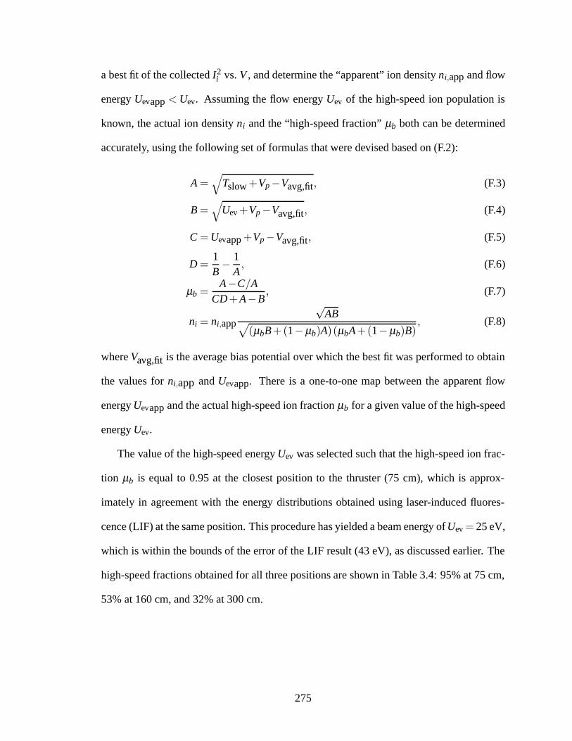
a best fit of the collected I2i vs. V , and determine the “apparent” ion density ni,app and flow
energy Uevapp <Uev. Assuming the flow energy Uev of the high-speed ion population is
known, the actual ion density ni and the “high-speed fraction” µb both can be determined
accurately, using the following set of formulas that were devised based on (F.2):
A=√
Tslow+Vp−Vavg,fit, (F.3)
B=√
Uev+Vp−Vavg,fit, (F.4)
C =Uevapp+Vp−Vavg,fit, (F.5)
D=1B−
1A, (F.6)
µb =A−C/A
CD+A−B, (F.7)
ni = ni,app
√AB√
(µbB+(1−µb)A)(µbA+(1−µb)B), (F.8)
where Vavg,fit is the average bias potential over which the best fit was performed to obtain
the values for ni,app and Uevapp. There is a one-to-one map between the apparent flow
energy Uevapp and the actual high-speed ion fraction µb for a given value of the high-speed
energy Uev.
The value of the high-speed energy Uev was selected such that the high-speed ion frac-
tion µb is equal to 0.95 at the closest position to the thruster (75 cm), which is approx-
imately in agreement with the energy distributions obtained using laser-induced fluores-
cence (LIF) at the same position. This procedure has yielded a beam energy of Uev= 25 eV,
which is within the bounds of the error of the LIF result (43 eV), as discussed earlier. The
high-speed fractions obtained for all three positions are shown in Table 3.4: 95% at 75 cm,
53% at 160 cm, and 32% at 300 cm.
275

F.1.1 Evaluation of the Error on Density Estimates
Typically, the error on Langmuir probe density measurement is estimated as the discrep-
ancy between the electron and ion densities. However, in the case of a flowing plasma, elec-
tron current collection is significantly enhanced, as is shown in chapter 3, a phenomenon
that no existing model can quantitatively predict, as discussed in Section 4.6. On the other
hand, the effect of flow on ion current collection is very well understood, which means that
plasma flow does not cause significant errors in the ion density estimates. Thus, the quan-
tity |ne−ni|would merely provide a measure of the error on the electron density introduced
by the plasma flow.
Given that plasma flow does not contribute a significant error to the ion density estimate,
the primary source of error in the determination of plasma density estimates is the error
on the Langmuir probe area estimate. We estimate the error on the length of the 4-cm
Langmuir probe to be about 1 mm. As for the Langmuir probe’s diameter of 0.28-mm, it
is much more accurate due to precision manufacturing; it is estimated to have a 0.01-mm
tolerance (actual tolerance could not be obtained from the manufacturer). Based on these
two errors, the relative error on the probe area can be computed as 1/40+0.01/0.28≈ 6%.
Now, the collected ion current is proportional to the product of the probe area and
plasma density. Thus, the 6% relative error on probe area contributes a 6% relative error
on our density estimates. Other, secondary sources of error, such as voltage and current
measurement errors, should certainly amount to less than 2%. A conservative error estimate
would thus be obtained by the sum of 6% and 2%, for a total of 8%.
276

F.2 Electron Retardation Analysis: Plasma Potential Vp
and Electron Temperature Te
Variations in the effective work function on the surface of our Langmuir probe (referred
to as work function patchiness by Brace [7]) has turned out to be an area of concern in our
experimental data. Our results appear to suggest a total effective work function variation
of several eV. Figure F.2 illustrates that effect, which leads to a departure from exponential
behavior before the plasma potential is attained. Possible explanations for this variation
could include polycrystalline workfunction variations of the Tungsten probes (on the order
of 1 eV, the Tungsten workfunction being on the order of 4.5 eV), and possible surface
contaminants, such as adsorbed residual gases and adsorbed xenon ions. A quantitative
assessment of the contamination sources is outside of the scope of the present paper, but
we note here that several authors have linked effective work function variations to surface
adsorbates [85–91].
A simple numerical experiment on the theoretical current collection curves was per-
formed in order to emulate the “blurring” effect of the work function variation. Figure F.3
shows the results of this numerical experiment in the “thin sheath” and “OML” limits. The
dashed curves, shown in both linear and semi-logarithmic formats, is the result of “blur-
ring” the theoretical curves using a local averaging window of width equal to 4.8 times
the electron temperature. The blurred thin sheath curve is shown to collect less than the
thermal current Ith at the plasma potential (V/Te=0 here), while on the blurred OML curve,
the collected current at plasma potential is still equal to the thermal current Ith. It turns out
that it will stay within 3% of Ith as long as the work function variation is under 6.7 times
the thermal temperature.
We use this feature of the OML blurring in our determination of the plasma potential.
In other words, we locate the plasma potential by finding the potential where the collected
277

−20 −15 −10 −5 0 5 10 15 20−14
−12
−10
−8
−6
−4
−2
0
Probe Bias (volts)
log(
I e/I the)
log(Ie/I
the) vs Probe Bias
Figure F.2: Best fits in the electron retardation regime of a transverse-flow Langmuir probe.Two linear best-fits are performed on this semi-log plot. The one occurring at lower poten-tial values corresponds to a population of warmer electrons, which account for just a fewpercent of the electron population.
current is equal to the electron thermal current. The cross-hair in Figure F.2 illustrates that
result. As for the electron temperature, we may safely determine it based on the inverse
of the slope of the retardation region within the linear part of FigureF.3(b), that is, beyond
the reach of the blurring effect of the work function variation, as the rightmost linear fit
shows in Figure F.2. The leftmost linear fit shown on the same figure is identified with a
population of warmer electrons, which account for just a few percent of the total electron
population.
278
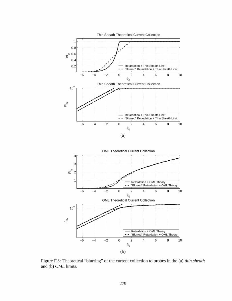
−6 −4 −2 0 2 4 6 8 10
0.2
0.4
0.6
0.8
1
φ0
I/Ith
Thin Sheath Theoretical Current Collection
Retardation + Thin Sheath Limit"Blurred" Retardation + Thin Sheath Limit
−6 −4 −2 0 2 4 6 8 10
100
φ0
I/Ith
Thin Sheath Theoretical Current Collection
Retardation + Thin Sheath Limit"Blurred" Retardation + Thin Sheath Limit
(a)
−6 −4 −2 0 2 4 6 8 10
1
2
3
4
φ0
I/Ith
OML Theoretical Current Collection
Retardation + OML Theory"Blurred" Retardation + OML Theory
−6 −4 −2 0 2 4 6 8 10
100
φ0
I/Ith
OML Theoretical Current Collection
Retardation + OML Theory"Blurred" Retardation + OML Theory
(b)
Figure F.3: Theoretical “blurring” of the current collection to probes in the (a) thin sheathand (b) OML limits.
279

F.2.1 Evaluation of the Error on Temperature Estimates
The temperature determination from the exponential fit of the retardation data is inde-
pendent of the probe area, and as a consequence, the error on the Langmuir probe area
estimate has no bearing on the accuracy of the temperature estimate. The primary sources
of error in the temperature determination are thus
• the relative accuracy of the voltages measured by the Keithley 2410 sourcemeter that
was used for the LP measurements, which is better than 1%; and
• the empirical process used to select the voltage range over which a best fit of the
retardation regime is performed.
In order to be conservative in accounting for both of these error terms, we will assume an
overall accuracy of 5% for our temperature estimates.
Because the Debye length estimate is determined based on the estimated density and
temperature values through the relationship λDe =√
ε0Teen0
, the relative accuracy on Debye
length, consistent with the 5% and 8% relative accuracy estimates for temperature and
density, is obtained from:
∆λDe
λDe=
12
(∆Te
Te+
∆nn
)=
12(5%+8%) = 6.5% (F.9)
280

BIBLIOGRAPHY
281

BIBLIOGRAPHY
[1] J. Sanmartın, M. Martınez-Sanchez, and E. Ahedo, “Bare wire anodes for electrody-namic tethers,” Journal of Propulsion and Power, vol. 9, no. 3, pp. 353–360, 1993.
[2] R. Estes, E. Lorenzini, J. Sanmartın, J. Pelaez, M. Martınez-Sanchez, C. Johnson, andI. Vas, “Bare tethers for electrodynamic spacecraft propulsion,” Journal of Spacecraftand Rockets, vol. 37, no. 2, pp. 205–211, March-April 2000.
[3] V. V. Danilov, V. V. Mirnov, and D. Ucer, “High-voltage space tether for enhancedparticle scattering in Van Allen belts,” Fusion Technology, vol. 35, no. 1T, pp. 312–314, January 1999.
[4] V. V. Danilov, B. Elgin, O. Grafodatsky, and V. Mirnov, “High-voltage satellite teth-ers for active experiments in space,” in Proceedings of the 6th Spacecraft ChargingTechnology Conference, AFRL–VS–TR–20001578, September 2000, pp. 165–168.
[5] Y. V. Vasil’yev and V. V. Danilov, “Proposal for an attempt to influence the precipita-tion of charged particles from the Earth’s radiation belts by means of a satellite-bornehigh-voltage cable system,” Transaction (Doklady) of the Russian Academy of Sci-ences: Earth Science Sections, vol. 345A, no. 9, pp. 172–176, October 1996.
[6] J. Laframboise and L. Parker, “Probe design for orbit-limited current collection,” ThePhysics of Fluids, vol. 16, no. 5, pp. 629–636, May 1973.
[7] L. H. Brace, Measurement Techniques in Space Plasmas: Particles. American Geo-physical Union, 1998, ch. Langmuir Probe Measurements in the Ionosphere, pp. 23–35.
[8] J. Laframboise, “Theory of spherical and cylindrical Langmuir probes in a collision-less, Maxwellian plasma at rest,” Ph.D. dissertation, University of Toronto, June 1966.
[9] S. G. Bilen, “Pulse propagation along conductors in low- density, cold plasmas asapplied to electrodynamic tethers in the ionosphere,” Ph.D. dissertation, University ofMichigan, 1998.
[10] I. E. Vas, T. J. Kelly, and E. A. Scarl, “Space station reboost with electrodynamictethers,” Journal of Spacecraft and Rockets, vol. 37, no. 2, pp. 154–164, March–April2000.
282

[11] J. Sanmartın and R. Estes, “The orbital-motion-limited regime of cylindrical Lang-muir probes,” Physics of Plasmas, vol. 6, no. 1, pp. 395–405, 1999.
[12] R. Estes and J. Sanmartın, “Cylindrical Langmuir probes beyond the orbital-motion-limited regime,” Physics of Plasmas, vol. 7, no. 10, pp. 4320–4325, October 2000.
[13] L. Johnson, B. E. Gilchrist, R. D. Estes, E. Lorenzini, and J. Ballance, “Propul-sive small expendable deployer system (ProSEDS) space experiment,” AIAA PaperAIAA–98–4035, 1998.
[14] J. V. Noord and R. Strumfels, “Electrodynamic tether optimization for the STEP-AirSEDS mission,” AIAA Paper AIAA–2001–3980, 2001.
[15] R. P. Hoyt and B. M. Minor, “Remediation of radiation belts using electrostatic tetherstructures,” 2004, Tethers Unlimited, Inc.
[16] J. Parmentola et al., “High altitude nuclear detonations against low Earthorbit satellites,” Defense Threat Reduction Agency, Advanced Systems andConcepts Office, U.S. Government,” Slides, April 2001. [Online]. Available:http://www.fas.org/spp/military/program/asat/haleos.pdf.
[17] G. Z. Xu, “The interation of a moving spacecraft with the ionosphere: Current collec-tion and wake structure,” Ph.D. dissertation, York University, 1992.
[18] J. Sanmartın and R. Estes, “Interference of parallel cylindrical Langmuir probes,”Physics of Plasmas, vol. 8, no. 9, pp. 4234–4239, September 2001.
[19] A. S. Jursa, Ed., Handbook of geophysics and the space environment. Air ForceGeophysics Laboratory, Air Force Systems Command, U.S. Air Force, 1985.
[20] R. Hoyt, B. Minor, J. Slostad, and N. Voronka, “Electrodynamic/electrostatic tetherperformance assessment program-tether payloads concept design, appendix H (elec-trostatic scattering model),” September 2003, TUI Final Report on DARPA/SPOSeedling Contract.
[21] D. Gallagher, P. Craven, and R. Comfort, “Global core plasma model,” Journal ofGeophysical Research, vol. 105, no. A8, pp. 18 819–18 833, August 2000.
[22] J. C. McMahon, “The interaction of infinite and finite cylindrical probes with a drift-ing collisionless Maxwellian plasma,” Ph.D. dissertation, York University, September2000.
[23] J. M. Quinn, R. J. Coleman, D. L. Shiel, and J. M. Nigro, “The joint US/UK 1995epoch world magnetic model,” Naval Oceanographic Office, Tech. Rep., 1995.
[24] J. M. Quinn, 1990, ”GEOMAG.for” and ”GEOMG1.for” Fortran subroutines for thecalculation of geomagnetic field based on the World Magnetic Model, Naval Oceano-graphic Office.
283

[25] M. A. Lieberman and A. J. Lichtenberg, Principles of Plasma Discharges and Mate-rials Processing. Wiley Interscience, 1994.
[26] H. Mott-Smith and I. Langmuir, “The theory of collectors in gaseous discharges,”Physical Review, vol. 28, pp. 727–763, 1926.
[27] I. Bernstein and I. Rabinowitz, “Theory of electrostatic probes in a low-densityplasma,” Physics of Fluids, vol. 2, no. 2, pp. 112–121, March-April 1959.
[28] M. Kanal, “Theory of current collection of moving cylindrical probes,” Journal ofApplied Physics, vol. 35, p. 1697, 1964.
[29] W. Hoegy and L. Wharton, “Current to a moving cylindrical electrostatic probe,”Journal of Applied Physics, vol. 44, no. 12, pp. 5365–5371, December 1973.
[30] R. Godard and J. Laframboise, “Total current to cylindrical collectors in collisionlessplasma flow,” Planetary and Space Science, vol. 31, no. 3, pp. 275–283, 1983.
[31] T. Onishi, “Numerical study of current collection by an orbiting bare tether,” Ph.D.dissertation, Massachusetts Institute of Technology, August 2002.
[32] A. Geist, A. Beguelin, J. Dongarra, W. Jiang, R. Manchek, and V. Sunderam, PVM3 User’s Guide and Reference Manual, Oak Ridge National Laboratory, September1994.
[33] C. Birdsall and A. B. Langdon, Plasma Physics Via Computer Simulation. IOPPublishing, 1991.
[34] F. Filbet and E. Sonnendrucker, “Comparison of Eulerian Vlasov solvers,” Comp.Phys. Comm., vol. 150, no. 3, pp. 247–266, 2003.
[35] L. Parker and E. Sullivan, “Numerical solution of the Poisson-Vlasov system for aspherical electrostatic probe,” SIAM Fall Meeting, October 1970.
[36] L. W. Parker, “Computation of collisionless steady-state plasma flow past a chargeddisk,” Lee W. Parker, Inc., Tech. Rep., 1976, prepared for NASA - George C. MarshallSpace Flight Center.
[37] M. Tautz, D. Cooke, A. Rubin, and G. Yates, “Preliminary documentation of theMACH code,” Hanscom Air Force Base, Tech. Rep., September 1987.
[38] F. F. Chen, Introduction to plasma physics and controlled fusion, 2nd ed. PlenumPress, 1984.
[39] P. M. Chung, L. Talbot, and K. J. Touryan, Electric Probes in Stationary and FlowingPlasmas: Theory and Application. Springler–Verlag, 1975.
[40] A. V. Gurevich, “Distribution of captured particles in a potential well in the absenceof collisions,” Soviet Physics JETP, vol. 26, no. 3, pp. 575–580, March 1968.
284

[41] M. Lampe, V. Gavrishchaka, G. Ganguli, and G. Joyce, “Effect of trapped ions onshielding of a charged spherical object in a plasma,” Physical Review Letters, vol. 86,no. 23, pp. 5278–5281, June 2001.
[42] F. Hecht, “Bidimensional anisotropic mesh generator,” INRIA (France), Tech. Rep.,1998.
[43] D. K. Cheng, Field and wave electromagnetics. Addison-Wesley Pub. Co., 1989.
[44] P. Tong and J. N. Rossettos, Finite-Element Method - Basic Technique and Imple-mentation. The MIT Press, 1977, ch. 2: The Finite-Element Method for Poisson’sEquation, pp. 40–71.
[45] C. Fox, An Introduction to the Calculus of Variations. Dover Publications Inc., 1987.
[46] W. R. Smythe, Static and Dynamic Electricity, 3rd ed. McGraw-Hill Book Company,1968.
[47] E. Kreysig, Advanced Engineering Mathematics, 7th ed. John Wiley & Sons, 1993.
[48] W. H. Press, S. A. Teukolsky, W. T. Vetterling, and B. P. Flannery, Numerical Recipesin C, 2nd ed. Cambridge University Press, 1992.
[49] L. C. Evans, Partial differential equations. American Mathematical Society, 1998.
[50] J. Bernstsen and T. O. Espelid, “Algorithm 706–DCUTRI: An algorithm for adap-tive cubature over a collection of triangles,” Transactions on Mathematical Software,vol. 18, no. 3, pp. 329–342, September 1992.
[51] T. O. Espelid, “Remark on algorithm 706: DCUTRI – An algorithm for adaptive cu-bature over a collection of triangles,” Transactions on Mathematical Software, vol. 24,no. 3, pp. 334–335, September 1998.
[52] K. A. Sikorski, Optimal Solution of Nonlinear Equations. Oxford University Press,2001.
[53] R. L. Burden, Numerical Analysis, 4th ed. PWS-KENT Publishing Company, 1989.
[54] L. N. Trefethen and I. David Bau, Numerical Linear Algebra. Society for Industrialand Applied Mathematics, 1997.
[55] A. Neumaier, “Solving ill-conditioned and singular linear systems: a tutorial on reg-ularization,” SIAM Review, vol. 40, no. 3, pp. 636–666, September 1998.
[56] C. Hansen, “Regularization tools – a Matlab package for analysis and solution ofdiscrete ill-posed problems,” Numerical Algorithms, vol. 6, pp. 1–35, 1994.
[57] C. Hansen, Regularization Tools – A Matlab Package for Analysis and Solution ofDiscrete Ill-Posed Problems. Department of Mathematical Modelling, TechnicalUniversity of Denmark, September 2001.
285

[58] A. Tikhonov, A. Goncharsky, V. Stepanov, and A. Yagola, Numerical Methods for theSolution of Ill-Posed Problems. Kluwer Academic Publishers, 1995.
[59] C. Kelley, Iterative Methods for Linear and Nonlinear Equations. Philadelphia:Society for Industrial and Applied Mathematics, 1995.
[60] H. W. Engl, M. Hanke, and A. Neubauer, Regularization of Inverse Problems.Kluwer Academic Publishers, 1996.
[61] S. Fridman, “Reconstruction of a three-dimensional ionosphere from backscatter andvertical ionograms measured by over-the-horizon radar,” Radio Science, vol. 33, no. 4,pp. 1159–1171, 1998.
[62] B. Kaltenbacher, “Some Newton-type methods for the regularization of nonlinear ill-posed problems,” Inverse Problems, vol. 13, pp. 729–753, 1997.
[63] J. Qi-Nian, “Applications of the modified discrepancy principle to Tikhonov regu-larization of nonlinear ill-posed problems,” SIAM Journal of Numerical Analysis,vol. 36, no. 2, pp. 475–490, 1999.
[64] A. Rieder, “On the regularization of nonlinear ill-posed problems via inexact Newtoniterations,” Inverse Problems, vol. 15, no. 1, pp. 309–327, February 1999.
[65] E. Haber and D. Oldenburg, “A GCV based method for nonlinear ill-posed problems,”Computational Geosciences, vol. 4, pp. 41–63, 2000.
[66] A. Rieder, “On convergence rates of inexact Newton regularizations,” NumericalMathemetics, vol. 88, pp. 347–365, 2001.
[67] V. Morozov, Methods for Solving Incorrectly Posed Problems. Springer-Verlag,1984.
[68] F. Hecht, BAMG: Bidimensional Anisotropic Mesh Generator, Institut National deRecherche en Informatique et en Automatique, Rocquencourt, 75153 Le Chenay,France, October 1998, edition 0.58.
[69] M. Castro-Dıaz, F. Hecht, B. Mohammadi, and O. Pironneau, “Anisotropic unstruc-tured mesh adaption for flow simulations,” International Journal for Numerical Meth-ods in Fluids, vol. 25, pp. 475–491, 1997.
[70] H. Borouchaki, P. L. George, F. Hecht, P. Laug, and E. Saltel, “Delaunay mesh gener-ation governed by metric specifications. Part I. Algorithms,” Finite Elements in Anal-ysis and Design, vol. 25, pp. 61–83, 1997.
[71] E. Choiniere, B. E. Gilchrist, S. G. Bilen, K. R. Furhrhop, and A. D. Gallimore,“Experimental investigation of electron collection to solid and slotted tape probes ina high-speed flowing plasma,” submitted for publication to the IEEE Transactions onPlasma Science in April 2004.
286
[72] B. E. Gilchrist, S. G. Bilen, E. Choiniere, A. D. Gallimore, and T. B. Smith, “Analysisof chamber simulations of long collecting probes in high-speed dense plasmas,” IEEETransactions on Plasma Science, vol. 30, no. 5, pp. 2023–2034, October 2002.
[73] J. M. Haas, F. S. G. II, A. D. Gallimore, G. G. Spanjers, and R. A. Spores, “Perfor-mance characteristics of a 5 kw laboratory Hall thruster,” AIAA Paper AIAA–98–3503, 1998.
[74] B. E. Gilchrist, S. Bilen, E. Choiniere, and A. D. Gallimore, “Laboratory experimentsof current collection to long tape probes using a high-speed plasma relevant to bareelectrodynamic tethers: Calibration and initial solid and slotted tape measurements,”University of Michigan, Tech. Rep., 2002.
[75] G. J. J. Williams, T. B. Smith, M. T. Domonkos, K. J. Shand, A. D. Gallimore, andR. P. Drake, “Laser induced fluorescence measurement of ion velocities in the plumeof a hall effect thruster,” AIAA Paper AIAA–99–2862, 1999.
[76] T. B. Smith, D. A. Herman, A. D. Gallimore, and R. P. Drake, “Deconvolution of axialvelocity distributions from Hall thruster LIF spectra,” Paper IEPC–01–0019 presentedat the 27th International Electric Propulsion Conference, 1999.
[77] E. Choiniere and B. E. Gilchrist, “Modeling long probes in flowing plasmas usingKiPS-2D, a novel steady-state Vlasov solver,” AIAA Paper AIAA–2003–5098, 2003.
[78] E. Choiniere and B. E. Gilchrist, “Electron collection to arbitrarily shaped electro-dynamic tethers in flowing plasmas: a kinetic model – validation for circular cross-sections,” AIAA Paper AIAA–2002–4050, July 2002.
[79] J. G. Laframboise, “Correction of one ion density data curve from [8, figure 33] forthe case r0 = λDe,” 1974, private Communication.
[80] W. J. Larson and J. R. Wertz, Space Mission Analysis and Design. Kluwer AcademicPublishers, 1992.
[81] D. Cooke and I. Katz, “TSS-1R electron currents: Magnetic limited collection from aheated presheath,” Geo. Res. Let., vol. 25, no. 5, pp. 753–756, March 1998.
[82] E. Choiniere, “Assessment of possible space charge effects caused by secondary elec-tron emission,” July 2004, technical Note.
[83] J. Laframboise, D. Wallis, and H. James, “RF effects on Oedipus-C floating voltages,”in Proceedings of the 8th Spacecraft Charging Technology Conference, 2003.
[84] G. E. Moore, “Cramming more components onto integrated circuits,” Electronics,vol. 38, no. 8, April 1965.
[85] G. Wehner and G. Medicus, “Reliability of probe measurements in hot cathode gasdiodes,” Journal of Applied Physics, vol. 23, no. 9, pp. 1035–1045, September 1952.
287

[86] C. Winkler, D. Strele, S. Tscholl, and R. Schrittwieser, “On the contamination ofLangmuir probe surfaces in a potassium plasma,” Plasmas Physics and ControlledFusion, vol. 42, pp. 217–223, 2000.
[87] B. Waclawski and L. Hughey, “Adsorption of water vapor on polychrystalline tung-sten,” Surface Science, vol. 19, pp. 464–468, 1970.
[88] M. J. Dresser, T. E. Madey, and J. John T. Yates, “The adsorption of xenon by W(111),and its interaction with preadsorbed oxygen,” Surface science, vol. 42, pp. 533–551,1974.
[89] H. Miki, H. Inomata, K. Kato, T. Kioka, and K. Kawasaki, “Chemisorption of NO onpolychrystalline tungsten surface,” Surface Science, vol. 141, pp. 473–486, 1984.
[90] T. Kioka, A. Kawana, H. Miki, S. Sugai, and K. Kawasaki, “Chemisorption of NO onW(100) and W(110) surfaces studies by AES and UPS,” Surface Science, vol. 182,pp. 28–40, 1987.
[91] E. Stamate and K. Ohe, “Influence of surface condition in Langmuir probe measure-ments,” Journal of Vacuum Science and Technology, vol. 20, no. 3, pp. 661–666,2002.
288