Theory and Design of Nonlinear Metamaterials
232
Theory and Design of Nonlinear Metamaterials by Alec Daniel Rose Department of Electrical and Computer Engineering Duke University Date: Approved: David R. Smith, Supervisor Matthew S. Reynolds Steven A. Cummer Jungsang Kim Daniel J. Gauthier Dissertation submitted in partial fulfillment of the requirements for the degree of Doctor of Philosophy in the Department of Electrical and Computer Engineering in the Graduate School of Duke University 2013
Transcript of Theory and Design of Nonlinear Metamaterials

Theory and Design of Nonlinear Metamaterials
by
Alec Daniel Rose
Department of Electrical and Computer EngineeringDuke University
Date:Approved:
David R. Smith, Supervisor
Matthew S. Reynolds
Steven A. Cummer
Jungsang Kim
Daniel J. Gauthier
Dissertation submitted in partial fulfillment of the requirements for the degree ofDoctor of Philosophy in the Department of Electrical and Computer Engineering
in the Graduate School of Duke University2013

Abstract
Theory and Design of Nonlinear Metamaterials
by
Alec Daniel Rose
Department of Electrical and Computer EngineeringDuke University
Date:Approved:
David R. Smith, Supervisor
Matthew S. Reynolds
Steven A. Cummer
Jungsang Kim
Daniel J. Gauthier
An abstract of a dissertation submitted in partial fulfillment of the requirements forthe degree of Doctor of Philosophy in the Department of Electrical and Computer
Engineeringin the Graduate School of Duke University
2013

Copyright c© 2013 by Alec Daniel RoseAll rights reserved except the rights granted by the
Creative Commons Attribution-Noncommercial Licence

Abstract
If electronics are ever to be completely replaced by optics, a significant possibility
in the wake of the fiber revolution, it is likely that nonlinear materials will play a
central and enabling role. Indeed, nonlinear optics is the study of the mechanisms
through which light can change the nature and properties of matter and, as a corol-
lary, how one beam or color of light can manipulate another or even itself within
such a material. However, of the many barriers preventing such a lofty goal, the nar-
row and limited range of properties supported by nonlinear materials, and natural
materials in general, stands at the forefront. Many industries have turned instead to
artificial and composite materials, with homogenizable metamaterials representing a
recent extension of such composites into the electromagnetic domain. In particular,
the inclusion of nonlinear elements has caused metamaterials research to spill over
into the field of nonlinear optics. Through careful design of their constituent ele-
ments, nonlinear metamaterials are capable of supporting an unprecedented range of
interactions, promising nonlinear devices of novel design and scale. In this context,
I cast the basic properties of nonlinear metamaterials in the conventional formalism
of nonlinear optics. Using alternately transfer matrices and coupled mode theory, I
develop two complementary methods for characterizing and designing metamaterials
with arbitrary nonlinear properties. Subsequently, I apply these methods in nu-
merical studies of several canonical metamaterials, demonstrating enhanced electric
and magnetic nonlinearities, as well as predicting the existence of nonlinear magne-
iv

toelectric and off-diagonal nonlinear tensors. I then introduce simultaneous design
of the linear and nonlinear properties in the context of phase matching, outlining
five different metamaterial phase matching methods, with special emphasis on the
phase matching of counter propagating waves in mirrorless parametric amplifiers and
oscillators. By applying this set of tools and knowledge to microwave metamateri-
als, I experimentally confirm several novel nonlinear phenomena. Most notably, I
construct a backward wave nonlinear medium from varactor-loaded split ring res-
onators loaded in a rectangular waveguide, capable of generating second-harmonic
opposite to conventional nonlinear materials with a conversion efficiency as high as
1.5%. In addition, I confirm nonlinear magnetoelectric coupling in two dual gap
varactor-loaded split ring resonator metamaterials through measurement of the am-
plitude and phase of the second-harmonic generated in the forward and backward
directions from a thin slab. I then use the presence of simultaneous nonlinearities
in such metamaterials to observe nonlinear interference, manifest as unidirectional
difference frequency generation with contrasts of 6 and 12 dB in the forward and
backward directions, respectively. Finally, I apply these principles and intuition to
several plasmonic platforms with the goal of achieving similar enhancements and con-
figurations at optical frequencies. Using the example of fluorescence enhancement in
optical patch antennas, I develop a semi-classical numerical model for the calculation
of field-induced enhancements to both excitation and spontaneous emission rates of
an embedded fluorophore, showing qualitative agreement with experimental results,
with enhancement factors of more than 30,000. Throughout these series of works, I
emphasize the indispensability of effective design and retrieval tools in understand-
ing and optimizing both metamaterials and plasmonic systems. Ultimately, when
weighed against the disadvantages in fabrication and optical losses, the results pre-
sented here provide a context for the application of nonlinear metamaterials within
three distinct areas where a competitive advantage over conventional materials might
v

be obtained: fundamental science demonstrations, linear and nonlinear anisotropy
engineering, and extremely compact resonant all-optical devices.
vi

To my family, with whom I share all my accomplishments, and to whom I owe
my character.
vii

Contents
Abstract iv
List of Tables xii
List of Figures xiii
Acknowledgements xxiii
1 Introduction to passive, tunable, and nonlinear metamaterials 1
1.1 Introduction to metamaterials . . . . . . . . . . . . . . . . . . . . . . 2
1.2 Competing routes to active and tunable metamaterials . . . . . . . . 5
1.2.1 Mechanical tuning . . . . . . . . . . . . . . . . . . . . . . . . 6
1.2.2 Phase transitions . . . . . . . . . . . . . . . . . . . . . . . . . 7
1.2.3 Nonlinearity . . . . . . . . . . . . . . . . . . . . . . . . . . . . 8
2 The nonlinear susceptibilities 11
2.1 Coupled-wave theory . . . . . . . . . . . . . . . . . . . . . . . . . . . 12
2.2 Second-order response . . . . . . . . . . . . . . . . . . . . . . . . . . 14
2.3 Third-order response . . . . . . . . . . . . . . . . . . . . . . . . . . . 16
3 Nonlinear susceptibility retrieval: transfer matrix method 18
3.1 Theory . . . . . . . . . . . . . . . . . . . . . . . . . . . . . . . . . . . 20
3.1.1 Overview of the transfer matrix method . . . . . . . . . . . . 21
3.1.2 Three- and four-wave mixing . . . . . . . . . . . . . . . . . . . 27
3.1.3 Nonlinear parameter retrieval . . . . . . . . . . . . . . . . . . 31
viii

3.2 Numerical Validation . . . . . . . . . . . . . . . . . . . . . . . . . . . 34
3.3 Application to Experiment . . . . . . . . . . . . . . . . . . . . . . . . 36
3.4 Conclusion . . . . . . . . . . . . . . . . . . . . . . . . . . . . . . . . . 40
3.5 Appendix: Derivation of the source fields . . . . . . . . . . . . . . . . 42
4 Nonlinear susceptibility retrieval: coupled mode theory 45
4.1 Derivation of the effective nonlinear susceptibilities . . . . . . . . . . 47
4.1.1 Coupled-mode equations for wave mixing processes in a peri-odic medium . . . . . . . . . . . . . . . . . . . . . . . . . . . 49
4.1.2 The effective second-order susceptibilities . . . . . . . . . . . . 53
4.1.3 The effective third-order susceptibilities . . . . . . . . . . . . . 61
4.2 Numerical examples . . . . . . . . . . . . . . . . . . . . . . . . . . . . 62
4.2.1 The split ring resonator . . . . . . . . . . . . . . . . . . . . . 63
4.2.2 Prototypical nonlinear magnetoelectric metamaterial . . . . . 65
4.3 Examples of nonlinear magnetoelectric phenomena . . . . . . . . . . . 67
4.3.1 Nonlinear interference . . . . . . . . . . . . . . . . . . . . . . 67
4.3.2 Electro-optic effects . . . . . . . . . . . . . . . . . . . . . . . . 70
4.4 Spatial dispersion in the nonlinear susceptibilities . . . . . . . . . . . 72
4.5 Symmetry considerations . . . . . . . . . . . . . . . . . . . . . . . . . 77
4.6 Conclusion . . . . . . . . . . . . . . . . . . . . . . . . . . . . . . . . . 79
4.7 Appendix: Derivation of the nonlinear susceptibilities in the presenceof spatial dispersion . . . . . . . . . . . . . . . . . . . . . . . . . . . . 81
5 Engineering the effective nonlinear susceptibilities 83
5.1 The nonlinear retrieval method for media with nonlinear polarizationand magnetization . . . . . . . . . . . . . . . . . . . . . . . . . . . . 84
5.2 Simulations and retrievals . . . . . . . . . . . . . . . . . . . . . . . . 89
5.2.1 The nonlinear electric-field-coupled resonator (ELC) . . . . . . 94
5.2.2 The nonlinear split-ring resonator (SRR) . . . . . . . . . . . . 96
ix

5.2.3 The nonlinear cut-wire medium . . . . . . . . . . . . . . . . . 97
5.2.4 The nonlinear I-beam structure . . . . . . . . . . . . . . . . . 99
5.3 Calculation of the nonlinear conversion efficiencies . . . . . . . . . . . 100
5.3.1 Second-harmonic generation . . . . . . . . . . . . . . . . . . . 101
5.3.2 Self-phase modulation . . . . . . . . . . . . . . . . . . . . . . 104
5.4 Anisotropy and poling in the effective nonlinear tensors . . . . . . . . 106
5.5 Appendix: Second-harmonic generation in a doubly nonlinear medium 112
6 Metamaterial phase matching 116
6.1 Wave-mixing and phase mismatch: an overview . . . . . . . . . . . . 117
6.2 Anomalous dispersion phase matching . . . . . . . . . . . . . . . . . 119
6.3 Birefringence phase matching . . . . . . . . . . . . . . . . . . . . . . 121
6.4 Quasi-phase matching . . . . . . . . . . . . . . . . . . . . . . . . . . 125
6.5 Negative-index phase matching . . . . . . . . . . . . . . . . . . . . . 128
6.6 Index-near-zero phase matching . . . . . . . . . . . . . . . . . . . . . 129
6.7 Conclusion . . . . . . . . . . . . . . . . . . . . . . . . . . . . . . . . . 131
6.8 Appendix: Quasi-phase matching in a continuous medium . . . . . . 132
7 Novel microwave nonlinear metamaterials 137
7.1 Overview of microwave nonlinear metamaterials . . . . . . . . . . . . 138
7.1.1 Circuit model . . . . . . . . . . . . . . . . . . . . . . . . . . . 139
7.1.2 Simulation . . . . . . . . . . . . . . . . . . . . . . . . . . . . . 141
7.1.3 Measurement . . . . . . . . . . . . . . . . . . . . . . . . . . . 142
7.2 Phase matching in a nonlinear negative-index medium . . . . . . . . 144
7.3 Prototypical nonlinear magnetoelectric metamaterial . . . . . . . . . 154
7.4 Nonlinear interference . . . . . . . . . . . . . . . . . . . . . . . . . . 160
x
8 Plasmonic platforms for the visible spectrum 170
8.1 Metal films for nonlinear enhancement . . . . . . . . . . . . . . . . . 171
8.2 Film-coupled nanoparticles for fluorescence enhancement . . . . . . . 174
8.2.1 Calculating rates and enhancements . . . . . . . . . . . . . . . 177
8.2.2 Fluorescence enhancement in film-coupled nanoparticles . . . . 180
8.2.3 Comparison with experiment . . . . . . . . . . . . . . . . . . . 185
9 Conclusion 192
A Clarification of contributions 196
Bibliography 198
Biography 209
xi

List of Tables
5.1 (Reproduced with permission from Ref. [84]. Copyright (2011) by theAmerican Physical Society.) Optimal lengths, efficiencies, and nor-malized efficiencies for SHG in each NLMM. The conversion efficien-cies are calculated using the value χ
(2)d = 20 pm/V for the nonlinear
dielectric, and assuming an input intensity of 40 MW/cm2. . . . . . . 103
5.2 (Reproduced with permission from Ref. [84]. Copyright (2011) bythe American Physical Society.) Optimal lengths and conversion effi-ciencies for SPM in each NLMM. The conversion rates are calculatedusing the value χ
(3)d = 10−20 m2/V2 for the nonlinear dielectric. . . . . 105
6.1 (Reproduced with permission from Ref. [83]. Copyright (2011) byThe Optical Society.) Directions of Propagation and CorrespondingPhase Matching Condition for the Four Co-linear Three-Wave MixingConfigurations . . . . . . . . . . . . . . . . . . . . . . . . . . . . . . . 119
xii

List of Figures
1.1 Illustrative sketch of the homogenization over individual charges andcurrents (arrows) inherent in the macroscopic version of Maxwell’sequations. . . . . . . . . . . . . . . . . . . . . . . . . . . . . . . . . . 3
1.2 The split ring resonator as a meta-atom, showing the current (blackarrow) induced by an incident light wave. . . . . . . . . . . . . . . . . 4
1.3 Illustrative sketch of (a) mechanical, (b) phase change, and (c) non-linear field-induced mechanisms for metamaterial tuning. . . . . . . . 5
3.1 (Reproduced with permission from Ref. [70]. Copyright (2010) by theAmerican Physical Society.) The system considered in this paper iscomposed of a central slab possessing an arbitrary electric nonlinear-ity of order α, bounded by two semi-infinite linear media. Incidenton this slab is an arbitrary number of normally-propagating planewaves. The boundary conditions at the fundamental frequencies (ωq)are presented on top (blue), while the boundary conditions at thenonlinear-generated frequency (ωnl) are shown below (red). . . . . . . 22
3.2 (Reproduced with permission from Ref. [70]. Copyright (2010) by theAmerican Physical Society.) Comparison of the amplitudes of trans-mitted (a) and reflected (b) waves generated by three-wave mixing ascalculated by the transfer matrix approach (lines) and finite elementsimulations (circles). . . . . . . . . . . . . . . . . . . . . . . . . . . . 35
3.3 (Reproduced with permission from Ref. [70]. Copyright (2010) bythe American Physical Society.) Comparison of the amplitudes oftransmitted (a) and reflected (b) waves generated by four-wave mixingas calculated by the transfer matrix approach (solid lines) and finiteelement simulations (circles). . . . . . . . . . . . . . . . . . . . . . . . 36
xiii

3.4 (Reproduced with permission from Ref. [70]. Copyright (2010) by theAmerican Physical Society.) Plot of the transmitted SFG magneticfield spectrum. The red (solid) line is the raw data from experiment,while the black (dahsed) line is the corresponding Fourier processedsignal used in the retrieval. . . . . . . . . . . . . . . . . . . . . . . . . 38
3.5 (Reproduced with permission from Ref. [70]. Copyright (2010) bythe American Physical Society.) Comparison of the experimentallyretrieved (black diamonds) and the theoretical (red line) second-ordernonlinear susceptibility of the VLSRR medium. . . . . . . . . . . . . 40
4.1 (Reproduced with permission from Ref. [82]. Copyright (2012) bythe American Physical Society.) (a) The unit cell of an example MMcomposed of high-dielectric spheres, illustrating the coordinate (~r) and
lattice (~R) vectors. (b) and (c) represent typical cross-sections of ~θ(~r)
and ~φ(~r), respectively, obtained from eigenfrequency simulations forspheres with ε/ε0 = 300 and diameter a/3 embedded in free-space,showing the expected electric and magnetic-type responses. . . . . . . 58
4.2 (Reproduced with permission from Ref. [82]. Copyright (2012) bythe American Physical Society.) (a) Nonlinear SRR used in validatingEq. (4.26). Plots of the SRR’s retrieved linear (b) and nonlinear (c)properties via both scattering and eigenfrequency simulations. Theeffective χ
(2)mmm(2ω;ω, ω) is retrieved by both the nonlinear transfer
matrix method and Eq. (4.26), showing excellent agreement. Thegrayed frequency bands where no data is plotted correspond to eitherthe FF or second-harmonic falling in the SRR’s stop band that extendsover a narrow range of frequencies above the magnetic resonance. . . 64
4.3 (Reproduced with permission from Ref. [82]. Copyright (2012) bythe American Physical Society.) (a) The doubly-split nonlinear SRRused for both the symmetric and anti-symmetric configurations. (b)The retrieved linear properties from eigenfrequency simulations. Thesecond-order susceptibilities of the symmetric (c) and anti-symmetric(d) SRRs for SHG, calculated via (4.22) through (4.29). Due to the
degenerate frequencies involved in SHG, χ(2)eem and χ
(2)eme are identical,
as are χ(2)mem and χ
(2)mme. (e) and (f) show field maps of resonant SHG
from infinite columns of symmetric and anti-symmetric SRRs, respec-tively. . . . . . . . . . . . . . . . . . . . . . . . . . . . . . . . . . . . 66
xiv

4.4 (Reproduced with permission from Ref. [82]. Copyright (2012) by theAmerican Physical Society.) The second-order susceptibilities of thesymmetric (a) and anti-symmetric (b) SRRs for DFG, calculated via(4.22) through (4.29), for ω3a/2πc = 0.087. (c) and (d) show fieldmaps of DFG from infinite columns of symmetric and anti-symmetricSRRs, respectively, in the nearly degenerate case. The comparablemagnitudes in the two dominant nonlinear susceptibilities leads to uni-directional DFG, favoring forward generation in the symmetric SRR,and backward generation in the anti-symmetric SRR. . . . . . . . . . 69
4.5 (Reproduced with permission from Ref. [82]. Copyright (2012) by theAmerican Physical Society.) The effective second-order susceptibilitiesof the symmetric (b) and anti-symmetric (c) SRRs under a staticelectric field, calculated via (4.40) through (4.43). . . . . . . . . . . . 72
4.6 (Reproduced with permission from Ref. [82]. Copyright (2012) bythe American Physical Society.) (a) Illustration of the unit cell forinvestigating spatial dispersion in the nonlinear properties, consistingof a thin nonlinear slab of thickness d embedded in a dielectric ma-trix with periodicity a. (b) The effective nonlinear susceptibilities,
assuming εr = 2, d/a = 0.01, χ(2)loc/ε0 = 100 pm/V, ω2 = 1.5ω1, and
ω3 = ω1 + ω2, as a function of ω3a/2πc. . . . . . . . . . . . . . . . . . 75
4.7 Illustration of symmetries in nonlinear metamaterials. (a) A cen-trosymmetric inclusion, the double-gap SRR, placed over a uniformnonlinear substrate for maximizing the polar second-order suscepti-bility tensors. (b) A centrosymmetric inclusion placed over an anti-symmetric nonlinear substrate for maximizing the axial second-ordersusceptibility tensors. (c) A non-centrosymmetric inclusion placedover a uniform substrate excludes neither polar nor axial second-ordersusceptibility tensors. . . . . . . . . . . . . . . . . . . . . . . . . . . . 78
5.1 (Reproduced with permission from Ref. [84]. Copyright (2011) by theAmerican Physical Society.) Sketch of the nonlinear retrieval processfor metamaterials with simultaneous higher-order electric and mag-netic susceptibilities. (a) The nonlinear scattering from an inhomo-geneous unit cell, measured from simulation or experiment. (b) Theequivalent three layer system composed of a homogenized nonlinearslab sandwiched between regions of vacuum. (c) The magnetic (top)and electric (bottom) subproblems. . . . . . . . . . . . . . . . . . . . 86
xv

5.2 (Reproduced with permission from Ref. [84]. Copyright (2011) by theAmerican Physical Society.) (a) An ELC embedded in a nonlineardielectric. (b) The electric field norm at the resonance frequency.(c) The retrieved linear properties. (d) Log-scale plot of the second-and third-order electric field localization factors (Eq. (5.15)). (e-j)The retrieved electric and magnetic higher-order susceptibilities andcorresponding material figures of merit, normalized by the nonlinearbulk dielectric: (e-g) are the second-order properties corresponding toSHG and (h-j) are the third-order properties corresponding to SPM.The real (solid blue curve) and imaginary (dashed green curve) partsare shown for the higher-order susceptibilities. . . . . . . . . . . . . . 92
5.3 (Reproduced with permission from Ref. [84]. Copyright (2011) by theAmerican Physical Society.) (a) An SRR embedded in a nonlineardielectric. (b) The electric field norm at the resonance frequency.(c) The retrieved linear properties. (d) Log-scale plot of the second-and third-order electric field localization factors (Eq. (5.15)). (e-j)The retrieved electric and magnetic higher-order susceptibilities andcorresponding material figures of merit, normalized by the nonlinearbulk dielectric: (e-g) are the second-order properties corresponding toSHG and (h-j) are the third-order properties corresponding to SPM.The real (solid blue curve) and imaginary (dashed green curve) partsare shown for the higher-order susceptibilities. . . . . . . . . . . . . . 95
5.4 (Reproduced with permission from Ref. [84]. Copyright (2011) by theAmerican Physical Society.) (a) A cut-wire medium embedded in anonlinear dielectric. (b) The electric field norm at 10 THz. (c) Theretrieved linear properties. (d) Log-scale plot of the second- and third-order electric field localization factors (Eq. (5.15)). (e-j) The retrievedelectric and magnetic higher-order susceptibilities and correspondingmaterial figures of merit, normalized by the nonlinear bulk dielectric:(e-g) are the second-order properties corresponding to SHG and (h-j)are the third-order properties corresponding to SPM. The real (solidblue curve) and imaginary (dashed green curve) parts are shown forthe higher-order susceptibilities. . . . . . . . . . . . . . . . . . . . . . 97
xvi

5.5 (Reproduced with permission from Ref. [84]. Copyright (2011) by theAmerican Physical Society.) (a) An I-beam structure embedded in anonlinear dielectric. (b) The electric field norm at 10 THz. (c) Theretrieved linear properties. (d) Log-scale plot of the second- and third-order electric field localization factors (Eq. (5.15)). (e-j) The retrievedelectric and magnetic higher-order susceptibilities and correspondingmaterial figures of merit, normalized by the nonlinear bulk dielectric:(e-g) are the second-order properties corresponding to SHG and (h-j)are the third-order properties corresponding to SPM. The real (solidblue curve) and imaginary (dashed green curve) parts are shown forthe higher-order susceptibilities. . . . . . . . . . . . . . . . . . . . . . 99
5.6 (Reproduced with permission from Ref. [119]. Copyright (2013) bythe American Institute of Physics.) Sketch of a Pockels cell composedfrom a nanoparticle-ONLO composite, with variable dimensions in-dicated (a). The gap size is controlled by the extent of the ONLOaround the nanorod, while we define the overlap as the percentageof the nanorod that coincides transversely with its nearest neighbors.Illustration of polymer ordering before (b) and after (c) a poling fieldis applied to the medium. . . . . . . . . . . . . . . . . . . . . . . . . 107
5.7 (a) Illustration of the nanorod-polymer array, with the basic rectan-gular unit-cell indicated by the dashed red box. Plot of the real (band c) and imaginary (d and e) parts of the effective indices for bothpolarizations. . . . . . . . . . . . . . . . . . . . . . . . . . . . . . . . 108
5.8 Schematic of the local fields (a and b) and estimate of the local fieldenhancement in the gaps between nanorods (c and d) for the twotransverse poling configurations. . . . . . . . . . . . . . . . . . . . . . 110
5.9 Magnitude of the Pockels coefficient figures of merit for the goldnanorod-ONLO array, (ninj)
3/2rijk, normalized by the figure of meritfor the ONLO itself, in dB. The plots are separated by row, corre-sponding to the two transverse poling configurations, shown schemat-ically: poling field along z (top row) and poling field along x (bottomrow). . . . . . . . . . . . . . . . . . . . . . . . . . . . . . . . . . . . . 112
xvii

6.1 (Reproduced with permission from Ref. [83]. Copyright (2011) by TheOptical Society.) A nonlinear metamaterial consisting of overlappingsilver bars embedded in a nonlinear dielectric, designed to operateas a birefringence phase matched MOPO. (a) Schematic of a singlelayer of the metamaterial, showing the propagation direction and anglerelative to the crystal axes. (b) The basic unit-cell of the metamaterial.(c) The retrieved extraordinary and ordinary indices of refraction. (d)Plot of the phase matched signal and idler frequencies as a function ofangle. (e) Real and imaginary parts of the retrieved nonlinear coefficient.123
6.2 (Reproduced with permission from Ref. [83]. Copyright (2011) byThe Optical Society.) (a) Diagram of the periodic poling techniqueemployed in Ref. [89] for the varactor-loaded split-ring resonatormedium, whereby the phase of the nonlinear coefficient is periodi-cally flipped by reversing the orientation of the nonlinear element ineach individual unit-cell. (b) Schematic of tunable parallel-I QPMdifference frequency generation in an active metamaterial Bragg cell.An external stimulus is used to produce a periodic variation in thelinear properties of the metamaterial with a tunable period Λ. . . . . 127
6.3 (Reproduced with permission from Ref. [83]. Copyright (2011) byThe Optical Society.) (a) Plot of the calculated coherence lengths forparallel-I (dashed purple) and anti-parallel-I (solid orange) second-harmonic generation in a negative-index waveguide. The index ofrefraction at the fundamental frequency is included (dotted black),showing the negative-index and index-near-zero regimes (vertical dashedlines). (b) Schematic of the nonlinear optical mirror effect in negative-index metamaterial. (c) Schematic of simultaneous QPM in a period-ically poled index-near-zero metamaterial. Si refers to the directionof energy flow of the ith wave. . . . . . . . . . . . . . . . . . . . . . . 130
7.1 Typical Q(V ) curve for a varactor diode, compared to a third-orderpower series expansion, with good agreement for low voltages. Whenloaded in the capacitive gap of a microwave metamaterial, the powerseries coefficients can be related to the metamaterial’s macroscopicsecond- and third-order polarization and magnetization [74]. . . . . . 138
7.2 Schematic of the transmission line used to characterize the microwavemetamaterial samples. . . . . . . . . . . . . . . . . . . . . . . . . . . 143
7.3 (Reproduced with permission from Ref. [89]. Copyright (2011) bythe American Physical Society.) Photograph of the waveguide withthe top removed, loaded with four identical sections of VLSRRs. Theinset shows an enlarged view of the NLMM unit-cell. . . . . . . . . . 146
xviii

7.4 (Reproduced with permission from Ref. [89]. Copyright (2011) by theAmerican Physical Society.) Plot of the magnitude of the retrieved(solid blue) and fitted (dashed green) transmittance (a) and second-order susceptibility (b) for a single-layer VLSRR slab. . . . . . . . . . 147
7.5 (Reproduced with permission from Ref. [89]. Copyright (2011) by theAmerican Physical Society.) Plot of the calculated coherence lengthsfor transmitted (blue) and reflected (green) SHG in the VLSRR loadedwaveguide. The dashed lines at 12 and 24 cm correspond to thetwo poling periods used in this letter, while the gray band indicatesnonlinear-optical mirror behavior. . . . . . . . . . . . . . . . . . . . . 149
7.6 (Reproduced with permission from Ref. [89]. Copyright (2011) bythe American Physical Society.) Diagram of the experimental setupemployed to measure the SH spectrums, depicting a cross-section ofthe VLSRR loaded aluminum waveguide. . . . . . . . . . . . . . . . . 150
7.7 (Reproduced with permission from Ref. [89]. Copyright (2011) bythe American Physical Society.) Comparison of the transmitted (solidblue) and reflected (dashed green) SHG powers when all sections arealigned. The right inset depicts the experimental configuration, andthe left inset shows the TMM calculation. . . . . . . . . . . . . . . . 151
7.8 (Reproduced with permission from Ref. [89]. Copyright (2011) bythe American Physical Society.) Comparison of the transmitted SHGpower when the varactors are aligned (solid blue) and when they areperiodically poled with Λ = 12 cm (dotted red). . . . . . . . . . . . . 152
7.9 (Reproduced with permission from Ref. [89]. Copyright (2011) bythe American Physical Society.) Comparison of the transmitted (solidblue and dotted red) and reflected (dashed green and dotted black)SHG power when the varactors are aligned and when they are period-ically poled with Λ = 24 cm, respectively. . . . . . . . . . . . . . . . . 153
xix

7.10 (Reproduced with permission from Ref. [76]. Copyright (2012) by theAmerican Institute of Physics.) Simulation and analysis of the VL-SRRs. (a) The effective real (solid lines) and imaginary (dashed lines)linear properties. (b) The electric field norm (shading) and current(arrows) induced in response to an applied electric field (left) or mag-netic field (right) at 0.97 GHz. (c) Illustration of the internal SHGprocess. Arrows indicate the relative directionality of the voltagesacross the varactors (white) and the varactors themselves (red). The‘×’ symbolize the product in Eq. (7.14). The effective second-order
response is thus selected by the varactor orientations: χ(2)mmm(2ω;ω, ω)
in the anti-symmetric VLSRR, and χ(2)emm(2ω;ω, ω) in the symmetric
VLSRR. . . . . . . . . . . . . . . . . . . . . . . . . . . . . . . . . . . 156
7.11 (Reproduced with permission from Ref. [76]. Copyright (2012) bythe American Institute of Physics.) (a) Schematic of the experimentalsetup used in measuring the SH signals from the VLSRR samples. (b)Photograph of the single-layer VLSRR samples. . . . . . . . . . . . . 157
7.12 (Reproduced with permission from Ref. [76]. Copyright (2012) bythe American Institute of Physics.) Measured (blue markers) andsimulated (dashed lines) SHG from the two VLSRR samples. Thereflected SH spectrums are plotted in the upper diagrams, while thephase differences between the transmitted and reflected SH signals areplotted below. For comparison, the insets illustrate SHG from thinhomogeneous sheets with the indicated nonlinearity. As expected, thesymmetric VLSRR shows behavior consistent with an effective second-order polarization, proportional to the square of the FF magnetic field. 158
7.13 (Reproduced with permission from Ref. [159]. Copyright (2013) bythe American Physical Society.) Graphical illustration of the non-linear parameter space. Insets depict nonlinear generation (arrowsindicate electric fields) from a thin nonlinear slab for four limitingcases, corresponding to the areas under the colored cones. When thesecond-order polarization (magnetization) is dominant, as in the ver-tical (horizontal) cones, the nonlinear generation resembles an electric(magnetic) dipole. When a second-order polarization and magneti-zation are present, however, the interference can favor nonlinear gen-eration in a particular direction, illustrated by the insets next to thediagonal cones. This is an oversimplification, however, as both thepolarization and magnetization are, in general, complex valued. . . . 161
xx

7.14 (Reproduced with permission from Ref. [159]. Copyright (2013) bythe American Physical Society.) (a) The nonlinear SRR proposed inRef. [82] for observation of nonlinear interference. Both electric (left)and magnetic (right) incident fields interact with the nonlinear dielec-tric, resulting in nonlinear magnetoelectric coupling. (b) Photographof the analogous VLSRRs from Ref. [76]. . . . . . . . . . . . . . . . . 162
7.15 (Reproduced with permission from Ref. [159]. Copyright (2013) bythe American Physical Society.) Second-order susceptibilities calcu-lated for symmetric and anti-symmetric nonlinear SRRs in Ref. [82]as a function of ωi/ωp = 1 − ωs/ωp, for ωp fixed at the SRR reso-nance. The resonant susceptibilities (involving the magnetic compo-nent of the pump field) are dominant over most of the spectrum ineach VLSRR, so that DFG is dominated by their interference, as inEqs. (7.18) and (7.20). The insets graphically illustrate the resultingnonlinear interference in each sample, with the optimum occurring inthe neighborhood of ωs ≈ ωi ≈ ωp/2. . . . . . . . . . . . . . . . . . . 166
7.16 (Reproduced with permission from Ref. [159]. Copyright (2013) bythe American Physical Society.) (a) Schematic of the experimentalsetup for measuring DFG. (b) Plots of the forward and backward ex-perimental DFG spectra generated by the symmetric VLSRRs (left)and the anti-symmetric VLSRRs (right). The unidirectionality of thespectra confirm the presence of strong nonlinear interference, as illus-trated in the insets. The solid lines show the results of simulations forcomparison. . . . . . . . . . . . . . . . . . . . . . . . . . . . . . . . . 167
8.1 (Reproduced with permission from Ref. [189]. Copyright (2013) byThe Optical Society.) Norms of the reflected (a) and transmitted (b)fields generated from a silver film in the Kretschmann configurationas a function of the incident angles of the two fundamental waves.Dashed lines denote the surface plasmon excitation conditions derivedfrom Eq. (8.3). (c, d) Generated field patterns at points I (c) and II(d). . . . . . . . . . . . . . . . . . . . . . . . . . . . . . . . . . . . . . 173
8.2 Diagram of the simulation domain used in exploring fluorescence withinthe film-coupled nanocube. Inset shows a cross-section, with dimen-sions and variables indicated. . . . . . . . . . . . . . . . . . . . . . . 175
8.3 Generic energy level diagram showing the quasi-two level system underconsideration. The rates and energies most critical to spontaneousemission are indicated. Straight lines denote radiative and absorptive(photonic) transitions, while the wavy lines represent non-radiativerelaxation. . . . . . . . . . . . . . . . . . . . . . . . . . . . . . . . . . 179
xxi

8.4 Simulated emissive properties of a 100 nm diameter silver nanospherelocated 5 nm over a silver film as a function of fluorophore position. . 181
8.5 Simulated emissive properties of a 100 nm diameter silver nanodisklocated 5 nm over a silver film as a function of fluorophore position. . 182
8.6 Averaged enhancements in the emissive properties of a silver nanodisklocated 5 nm over a silver film for various disk diameters, plotted asa function of resonant wavelength. . . . . . . . . . . . . . . . . . . . . 183
8.7 Averaged enhancements in the emissive properties of a silver nan-odisk over a silver film for various disk diameters and gap thicknesses,constrained such that the resonant wavelength is fixed at 632.8 nm,plotted as a function of gap thickness. . . . . . . . . . . . . . . . . . . 184
8.8 (a) Schematic of the plasmonic nanopatch antenna platform, consist-ing of colloidally synthesized nanocubes dispersed over a silver filmand separated by a fluorophore-coated spacer layer. (b) Comparisonof typical plasmonic enhancement systems. The top row shows thegeometry and resonant electric field distribution, while the bottomrows describe the plasmonic systems qualitatively through effectiveand image dipoles and radiation patterns. . . . . . . . . . . . . . . . 185
8.9 (Reproduced with permission from Ref. [208].) Nanopatch scatteringand fluorescence enhancement. (a) Dark-field microscope image ofthe nanopatches under white-light illumination. The dominant colorof each nanopatch corresponds to the resonant wavelength (λ0) of itscavity mode. (b) Normalized scattering spectrum for two nanopatches.(c) Fluorescence enhancement factor for individual nanopatches as afunction of nanopatch resonance. The inset shows a typical fluores-cence spectra from a nanopatch. Laser excitation (λex, vertical line)and Cy5 in-solution emission spectra (shaded region) are shown forcomparison. . . . . . . . . . . . . . . . . . . . . . . . . . . . . . . . . 188
8.10 Plot of the averaged fluorescence enhancment factor versus resonantwavelength in log-scale. The data is fit with a piece-wise linear func-tion to determine a rough estimate of the variance in the measureddata. This variance in turn is used in analyzing the goodness-of-fit ofthe simulations with the measured data, as shown in Fig. 8.9. . . . . 189
8.11 The simulated excitation, radiative, and non-radiative rates as a func-tion of nanopatch resonant wavelength. The internal decay rate ofCy5, γ0
nr ≈ 5γ0r , is shown to be negligible by comparison. . . . . . . . 191
xxii

Acknowledgements
I gratefully acknowledge that these works would not have been possible without the
guidance of David R. Smith, and also Daniel Gauthier, as well as inventive support
and contributions from Stephane Larouche, Ekaterina Poutrina, Da Huang, Cris-
tian Ciracı, Xiaojun Liu, Guy Lipworth, and Nathan Landy. In addition, I would
like to thank the members of David Smith’s group and the Center for Metamateri-
als and Integrated Plasmonics for the many informal discussions and collaborative
environment that ultimately fostered this research.
The works presented here were supported in part by the Air Force Office of
Scientific Research (contract number FA9550-09-1-0562) and the U.S. Army Research
Office (grant # W911NF-12-1-0333).
xxiii

1
Introduction to passive, tunable, and nonlinearmetamaterials
Despite the seemingly diverse forms that natural materials take, whether texture,
color, or room-temperature phase, their physical properties tend to occupy only a
very narrow segment in a much wider spectrum. This is true whether we consider
electromagnetic, mechanical, or thermal properties. There is no better testament
to this lack of diversity in natural materials than the steadily increasing market for
composite materials. Once reserved for spacecraft, composites make up roughly 50%
of the Boeing 787 by weight. Composites have allowed bike frames to weigh less than
1 kg while retaining their stiffness. They show up in next generation prosthetics and
vehicle armor.
Metamaterials represent a natural extension of composite materials engineering
to electromagnetics. For example, fundamentally speaking, there is only one key
difference in whether magnetic flux is carried in the orbit of a single electron about a
nucleus, or by a sea of electrons following a closed conductive loop: the latter effect
can be far, far stronger. Simply put, there is much greater freedom in patterning
materials to form meta-atoms, and arranging these meta-atoms into metamaterials,
1

than exists in the natural world. In the early stages, the novel properties displayed
by metamaterials spurred research into a wide range of newly-achievable phenomena.
The resulting demonstrations attracted a large amount of excitement and attention,
but were ultimately fundamental, rather than application-oriented. As the field
has matured, however, researchers have started to revisit well-known problems in
industry, using the tools of metamaterial engineering to try and improve on existing
solutions in communications, imaging, and energy harvesting, to name a few.
1.1 Introduction to metamaterials
In the context of electromagnetics, a material’s response to an incident set of electric
and magnetic fields is a composition of the discrete charges and currents that are
carried by its basic atoms and molecules. For an exact solution of the fields, one would
need to take into account the contribution from each individual particle. However,
under the right conditions, certain approximations can be used to homogenize the
material response, neglecting the microscopic details in favor of locally averaged,
macroscopic fields. In this way, the numerous discrete charges and currents can
be simply replaced by effective parameters. This is essentially the approximation
inherent in the macroscropic version of Maxwell’s equations. The errors incurred are
negligible as long as the length scale of the averaging is much larger than the length
scale of the material’s inhomogeneity. In practice, this translates to the constraint
that a material’s internal structure is much smaller than the particular wavelength
of radiation. Nearly all natural materials satisfy this constraint well into the visible
spectrum, as the length scales of their internal structure are on the order of atomic
and molecular interactions. But at no point is it assumed that atoms and molecules
are the only constituents that can be described in this way.
As opposed to natural materials, the charges and currents that constitute the
electromagnetic response of a metamaterial are carried by the patterns and particles
2

Figure 1.1: Illustrative sketch of the homogenization over individual charges andcurrents (arrows) inherent in the macroscopic version of Maxwell’s equations.
of their internal structure. Thus, in exact analogy to natural materials, metamate-
rials can be described by homogeneous, constitutive parameters. But these patterns
and particles can behave very differently from their atomic counterparts. This allows
metamaterials to achieve properties that are either limited or entirely unachievable
in naturally occurring materials. A medium composed of split ring resonators like
that shown in Fig. 1.2, for example, can couple to incident magnetic fields to pro-
duce a region of negative permeability: a property not typically found in natural
materials [1].
Several different phenomena have been demonstrated for the first time in meta-
materials. In general, these involve the ability of metamaterials to achieve a wide
range of simultaneous values for their electric permittivity, magnetic permeability,
and magnetoelectric susceptibility tensors [2, 1, 3], as defined by the macroscopic
polarization and magnetization
~P (ω) = ε0 ¯χ(1)e (ω) ~E(ω) + i¯κ(1)(ω) ~H(ω), (1.1)
µ0~M(ω) = µ0 ¯χ(1)
m (ω) ~H(ω)− i[¯κ(1)(ω)
]∗ ~E(ω), (1.2)
respectively, where ε0 and µ0 are the permittivity and permeability of free-space, ω
is an angular frequency, ¯χ(1) are the rank-2 linear susceptibility tensors, and ¯κ is the
rank-2 linear magnetoelectric coupling tensor. Through the combination of these
responses, metamaterials have led to the demonstration of a variety of novel and
3

anomalous properties, including negative refraction [4, 5] and cloaking [6, 7, 8].
Figure 1.2: The split ring resonator as a meta-atom, showing the current (blackarrow) induced by an incident light wave.
Alongside the numerous demonstrations and fast paced research, new tools of
analysis and characterization have been developed specifically for metamaterials. In
particular, there exist several methods of homogenization for assigning appropriate
effective parameters to a particular engineered structure. In essence, the retrieval
process equates the unit cell of the metamaterial to a congruently sized homogeneous
material with an unknown set of electromagnetic properties. In the linear case, the
system is commonly solved by finding the equivalent permittivity, permeability, and
magneto-electric coefficient that replicate the scattering parameters of the metama-
terial [9, 10, 11]. This retrieval method has the added advantage of being easily ap-
plicable in practice through transmission and reflection experiments. Alternatively,
constitutive parameters can be determined through the process of field averaging,
but this technique is limited to cases where the local fields are known over the whole
of a unit cell [12]. Another tool often associated with metamaterials is the material
design methodology of transformation optics, wherein coordinate transformations are
implemented in Maxwell’s equations to prescribe the material parameters necessary
for a particular manipulation of the fields [13, 3].
4

1.2 Competing routes to active and tunable metamaterials
In addition, there exists a particular trait singular to resonant metamaterials, or
metamaterials whose electromagnetic response is based around a resonant compo-
nent or geometry. It was observed early on that these metamaterials, when operated
near resonance, displayed highly non-uniform field distributions over a unit cell [2].
The extreme variation in the field density implies that these structures exhibit sig-
nificant confinement of electromagnetic energy in small, critical volumes. This prop-
erty of resonant metamaterials has spurred the hybridization of metamaterials with
various functional materials, such as gain media, ferromagnets, piezoelectrics, and
numerous other candidates, imbuing the metamaterial as a whole with the properties
of the constituent material. This has led to the exciting demonstration of tunable
metamaterials, that is, metamaterials whose properties can be dynamically and re-
versibly controlled as a part of an active device. In what follows, we discuss several
potential routes towards tunable metamaterials (see, for example, Fig. 1.3). In par-
ticular, we develop this context for the introduction of metamaterials hybridized with
nonlinear materials, which are shown to occupy an important niche within tunable
metamaterials as a whole.
Figure 1.3: Illustrative sketch of (a) mechanical, (b) phase change, and (c) nonlin-ear field-induced mechanisms for metamaterial tuning.
5

1.2.1 Mechanical tuning
Perhaps the most obvious form of metamaterial tuning is mechanical. Metamaterial
elements are highly sensitive to their microscopic structure, such that any small
deformation to the geometry will be amplified in the metamaterial’s ability to reflect,
absorb, or refract radiation [14, 15, 16].
Often, mechanical tuning exploits the freedom in positioning the lattice substrate
itself. Lapine textslet. al. , for example, demonstrated continuous tuning of the
metamaterial resonance for lateral shifts between successive planes of microwave
resonators [17]. Similar designs have been tested at THz frequencies, relying on the
near-field coupling between successive elements [18]. However, these designs are not
suitable for dynamic tuning. Instead, it is preferential to have a mechanism by which
the substrate or housing can be deformed post-fabrication.
To this end, Li et. al. tuned the resonance of embedded metamaterial resonators
by more than 8% by applying strain directly to a highly elastic substrate [19]. Alter-
natively, planar metamaterial elements have been divided across two mechanically
separate but interlocked substrates, such that the internal unit-cell spacings can be
controlled by an externally applied voltage [20, 21, 22], or by local heating [23].
Microactuators have also proven useful components for changing the most sensitive
inter-element spacings (see, for example, Ref. [24] and Refs. within).
Clearly, the ability to reconfigure the geometry of metamaterial elements on the
order of the interparticle spacings grants immense control over the metamaterial
properties. However, such designs can be difficult to scale to the spacings necessary
for near-infrared and visible wavelengths. Instead, the rearrangement supported
by liquid crystals has been used to change the local electromagnetic environment
in the near-field of metamaterial elements [25, 26, 27, 28]. However, mechanical
reconfiguration is inherently a slow process, limited to switching on the order of
6

microseconds.
1.2.2 Phase transitions
Alternatively, certain materials are known to exhibit phase transitions in their op-
tical properties for different arrangements of their constituent atoms and molecules.
Hybridization of such phase transition materials with metamaterials can both lo-
calize external stimuli, such as heat or light, within the phase transition material,
and enhance the effect of the phase transition on the overall optical properties. As
before, the presence of a small amount of phase transition material can imbue the
entire metamaterial structure with similar but enhanced properties.
For example, vanadium dioxide has proven a popular choice as a phase transition
substrate, transitioning from an insulator to a conductor at a critical temperature.
When coupled to metamaterial resonators, the resonance can be extinguished by
vanadium dioxide’s conducting state, induced through heating of the entire struc-
ture [29, 30], application of an electrical pulse [31], or even through interaction with
a high-field terahertz pulse [32].
Semiconductor chalcogenide glasses, on the other hand, are widely used in phase
change rewriteable applications [33], owing to the large change in band-gap and
conductivity associated with its easily accessible amorphous-crystalline transition.
Plasmonics and metamaterial switches based around this phase transition have re-
cently been demonstrated [34, 35, 36], with the potential for switching speeds on the
order of 10s of nanoseconds.
Phase transition metamaterials like those listed above combine large, reversible,
optically induced tuning with modulation speeds that are much faster than their me-
chanically tuned counterparts. However, the speeds are still too slow for applications
in all-optical communication networks.
7

1.2.3 Nonlinearity
A nonlinear material is one whose electromagnetic response, i.e. the material’s polar-
ization and magnetization in the presence of electric and magnetic fields, cannot be
satisfactorily described by a linear proportionality with the incident fields. In fact,
all materials have a nonlinear response for sufficiently strong incident fields. How-
ever, the important characteristic is that the nonlinear response is fast, such that
the material responds at frequencies of the same order as the applied light. This
kind of ultrafast response is unique to the nonlinear mechanism, and allows not only
ultrafast switching times by using pump and probe light pulses, but can even induce
changes in the frequency of an incident wave.
A defining feature of linear systems is the principle of superposition, or the fact
that the output of a linear system from multiple inputs is equivalent to a sum of
the outputs from each input individually. Nonlinear responses, or equivalently the
higher-order terms in Eqs. (2.1) and (2.2), break this property, meaning that the
output of a nonlinear system for a particular input can be changed by adding addi-
tional inputs. The violation of superposition is a driving force in many applications
of nonlinear materials, and can allow for frequency generators and amplifiers in those
frequency ranges that currently lack lasers [37], high-speed switches in communica-
tion networks [38, 39], and even sub-diffraction-limit imaging [40, 41].
Most importantly, however, nonlinear processes like difference frequency genera-
tion and amplification are phase sensitive, coherent processes, in which the output
photons maintain a fixed phase relationship to the input photons. As such, nonlinear
materials are the main source of squeezed and entangled light [42, 43, 44, 45], and a
critical part of quantum information science [46].
Some of the most popular natural nonlinear materials for current nonlinear op-
tics technologies include ferroelectrics, semiconductors, organic polymers, and cer-
8

tain glasses [47, 48]. However, the nonlinear responses of such materials are so
weak that the subsequent devices typically require pulsed laser operation over long
interaction lengths, further limiting the materials of choice to those that can be
phase matched over long distances with small loss tangents and high damage thresh-
olds [49]. Metal films offer a interesting alternative due to the much larger nonlinear
responses that they possess [50, 51, 52, 53], but do not support bulk propagating
waves and suffer from large ohmic losses. Thus, much of the nonlinear metamate-
rial research has focused on nanostructuring metals in such a way to enhance their
already large nonlinearities while allowing the incident fields to couple in and out of
the structure [54, 55, 56]. For example, second-harmonic generation (SHG) has been
demonstrated from gold split-ring resonators, carefully controlling the polarization of
the incident fields and induced dipoles to ensure efficient re-radiation of the second-
harmonic [57, 58]. The third-order process of phase-conjugation has likewise been
measured from metal nanostructures [41]. On the other hand, the nonlinearities of
a substrate can themselves be enhanced by simple dielectric composites [59, 60] and
by metal patterning [38, 61]. By relying on light localization in the substrate rather
than the metal, such composites can potentially limit the effects of metallic losses
while still achieving large nonlinearities.
Due to its ultrafast response and phase coherency, the nonlinear mechanism for
tunable metamaterials deserves unique attention, with exciting applications as ul-
trafast optical switches, frequency generators, amplifiers, and sources of entangled
photons for quantum information science [15]. To address the complexity of nonlinear
metamaterials, with the hope of facilitating their design and application, the con-
tents of this thesis are as follows: I introduce the formalism for describing nonlinear
metamaterials in the context of conventional nonlinear optics in chapter 2. I develop
the primary experimental and analytic tools for the design and characterization of
nonlinear metamaterials in chapters 3 and 4. Next, I summarize and demonstrate
9

the two primary design strategies for nonlinear metamaterials: nonlinear suscepti-
bility engineering, and phase matching, in chapters 5 and 6, respectively. In chapter
7, I present the experimental observation of several novel nonlinear phenomena in
microwave metamaterials. Finally, in chapter 8, I extend the principles of nonlinear
metamaterial engineering to the related field of plasmonics. Chapter 9 summarizes
the presented material, offering my outlook for nonlinear metamaterials, their ad-
vantages and potential problems, and which applications are most likely to have a
major impact.
10

2
The nonlinear susceptibilities
We focus here on materials that are linear in the limit of weak incident fields. For
such materials, the polarization and magnetization can be expanded in a power-
series, such that
~P (t) = ~P (1)(t) + ~P (2)(t) + ~P (3)(t) + . . . (2.1)
and
~M(t) = ~M (1)(t) + ~M (2)(t) + ~M (3)(t) + . . . (2.2)
where the superscript denotes the dependence on the fields, i.e. linear, quadratic,
cubic, etc. We will divide our attention between two categories of nonlinear responses,
namely second- and third-order, and the phenomena associated with each. Bulk
second-order responses, mediated by ~P (2)(t) and ~M (2)(t), are associated with non-
centrosymmetric materials, or materials that possess no inversion symmetry. Third-
order responses, mediated by ~P (3)(t) and ~M (3)(t), can occurr in both centrosymmetric
and non-centrosymmetric media. Furthermore, it is convenient to investigate the
related phenomena in the frequency domain, for which we use the expansion
~E(t) =∑n
~E(ωn)e−iωnt, (2.3)
11

and likewise for the other field quantities, where the summation is over both positive
and negative frequencies. To satisfy the reality of the total fields, it follows that
~E(ωn) =[~E(−ωn)
]∗.
2.1 Coupled-wave theory
Nonlinear parametric processes, to which the majority of this thesis is devoted, are
best understood intuitively within the context of coupled-wave theory [62, 63, 64].
It is typically the case that the nonlinear response–even for most metamaterials–is
relatively small compared with the material’s linear response. The nonlinearity can
then be treated as a perturbation, so that we can at least retain the intuition and
language that we associate with linear wave propagation in a particular medium.
In particular, in source-free media, Maxwell’s macroscopic curl equations for the
fields at frequency ω in the presence of perturbations to both the polarization and
magnetization are
∇× ~E = iω[~B + µ0
~M (n)], (2.4)
∇× ~H = −iω[~D + ~P (n)
], (2.5)
with the constitutive relations
~D = ¯ε ~E + i¯κ ~H, (2.6)
~B = ¯µ ~H − i¯κ∗ ~E. (2.7)
Meanwhile, we know that, in the absence of the perturbation, the fields satisfy
∇× ~Eµ = iω ~Bµ, (2.8)
∇× ~Hµ = −iω ~Dµ, (2.9)
where we take ~Eµ and ~Hµ to represent the fields of some unperturbed mode µ with
unitary amplitude. Assuming purely real material properties, we follow the path
12

outlined in Ref. [64], combining Eqs. (2.4) through (2.9) to give
~H∗µ ·[∇× ~E
]− ~E ·
[∇× ~Hµ
]∗= iω ~H∗µ ·
[~B + µ0
~M (n)]− iω ~E · ~D∗µ (2.10)
and
~H ·[∇× ~Eµ
]∗− ~E∗µ ·
[∇× ~H
]= −iω ~H · ~B∗µ + iω~E∗µ ·
[~D + ~P (n)
]. (2.11)
Adding Eqs. (2.10) and (2.11), we can apply some vector calculus identities to obtain
∇ ·[~E × ~H∗µ + ~E∗µ × ~H
]= iω
[~P (n) · ~E∗µ + µ0
~M (n) · ~H∗µ]. (2.12)
From here, the coupled-mode equations can be found by choosing an explicit form
for the fields ~E and ~H and the perturbations ~P (n) and ~M (n).
In particular, for a linear homogeneous medium, we typically discuss propagation
in terms of a set of transverse electromagnetic (TEM) plane waves. Using the wave
label µ to denote frequency, polarization, and direction, we can write these waves
through the electric field
~Eµ = Aµ~eµei~kµ·~r (2.13)
and magnetic field
~Hµ = Aµ~hµei~kµ·~r (2.14)
where Aµ is the wave amplitude, and ~eµ and ~hµ are the corresponding polarization
vectors. We can normalize the polarization vectors according to
1
2
(~eµ × ~h∗µ + ~e∗µ × ~hµ
)= sµ, (2.15)
where sµ is the unit-normal in the direction of the Poynting vector. For this normal-
ization, the wave intensity is given simply by Iµ = 2Re(~Eµ × ~H∗µ
)= 2|Aµ|2. Using
this form for wave µ, we can reduce Eq. (2.12) to
∇Aµ(~r) · sµ = iωµ
[~P (n) · ~e∗µ + µ0
~M (n) · ~h∗µ]e−i
~kµ·~r. (2.16)
13

Thus, wave propagation can still be described through the medium’s linear modes
and waves, while the various amplitudes evolve in space according to a forcing term
proportional to the nonlinear perturbations. This expression can be extended to
include pulse dynamics [65], but is sufficient for illustrating the various nonlinear
processes, both in homogeneous media and metamaterials.
2.2 Second-order response
Expanding the fields in the frequency domain allows us to write the second-order re-
sponse of a medium in terms of eight independent second-order susceptibility tensors
of rank-3, as given by the following definitions of the second-order polarization,
~P (2)(t) =∑qr
[¯χ(2)eee(ωs;ωq, ωr) : ~E(ωq) ~E(ωr) + ¯χ(2)
emm(ωs;ωq, ωr) : ~H(ωq) ~H(ωr)+
¯χ(2)eem(ωs;ωq, ωr) : ~E(ωq) ~H(ωr) + ¯χ(2)
eme(ωs;ωq, ωr) : ~H(ωq) ~E(ωr)
]exp(−iωst), (2.17)
and second-order magnetization,
µ0~M (2)(t) =
∑qr
[¯χ(2)mmm(ωs;ωq, ωr) : ~H(ωq) ~H(ωr) + ¯χ(2)
mee(ωs;ωq, ωr) : ~E(ωq) ~E(ωr)+
¯χ(2)mme(ωs;ωq, ωr) : ~H(ωq) ~E(ωr) + ¯χ(2)
mem(ωs;ωq, ωr) : ~E(ωq) ~H(ωr)
]exp(−iωst).
(2.18)
It is evident that, in such a medium, the fields at one frequency will drive responses
at other frequencies, constituting what is known as three-wave mixing. In this way,
energy in the medium can be transfered between different frequencies, subject to the
constraint
ωq + ωr = ωs. (2.19)
If we consider the wave-mixing in terms of photons, we see that this is a statement of
energy conservation, as a photon’s energy is just ~ω, where ~ is the reduced Planck
constant.
14

As an example, using coupled-wave theory, we can consider the effect of waves
1 and 2, with frequencies ω1 and ω2, respectively, on wave 3 at the sum frequency
ω3 = ω1 + ω2, according to
∇ ·[A3
(~e3 × ~h∗3 + ~e∗3 × ~h3
)]= iω3
[~P (2) · ~e∗3 + ~M (2) · ~h∗3
]e−i
~k3·~r. (2.20)
If we assume a purely electric nonlinearity, such that
~P (2) = 2¯χ(2)eee : ~E1
~E2 = 2A1A2 ¯χ(2)eee : ~e1~e2e
i(~k1+~k2)·~r, (2.21)
and neglect ~M (2), the coupled-wave equation takes the familiar form [64]
∇A3(~r) · s3 = iω3 ¯χ(2)eee : ~e1~e2 · ~e∗3A1(~r)A2(~r)ei(
~k1+~k2−~k3)·~r. (2.22)
For self-consistency, these equations can be derived for all three interacting waves,
and solved for various configurations [66].
Thus, the second-order susceptibilities are responsible for sum frequency genera-
tion, second-harmonic generation (ω1 = ω2), difference frequency generation (ω1 or
ω2 < 0), optical parametric amplification (a particular case of difference frequency
generation in which a weak signal wave 3 is provided at the input), and the Pockels
effect (ω1 = 0, corresponding to a static electric field, and ω2 = ω3, such that the
static field changes the propagation of wave 3). But in any case, the key features
influencing energy transfer and wave manipulation, such as the polarization of the
various interacting waves, and phase matching, are evident in Eq. (2.22).
15

2.3 Third-order response
Analogous to the second-order material responses of Eqs. (2.17) and (2.18), let us
consider third-order polarization and magnetization of the forms
~P (3)(t) =∑pqr
[¯χ(3)eeee(ωs;ωp, ωq, ωr) : ~E(ωp) ~E(ωq) ~E(ωr)
+ ¯χ(3)eemm(ωs;ωp, ωq, ωr) : ~E(ωp) ~H(ωq) ~H(ωr)
+ ¯χ(3)eeem(ωs;ωp, ωq, ωr) : ~E(ωp) ~E(ωq) ~H(ωr)
+ ¯χ(3)eeme(ωs;ωp, ωq, ωr) : ~E(ωp) ~H(ωq) ~E(ωr)
+ ¯χ(3)emee(ωs;ωp, ωq, ωr) : ~H(ωp) ~E(ωq) ~E(ωr)
+ ¯χ(3)emmm(ωs;ωpωq, ωr) : ~H(ωp) ~H(ωq) ~H(ωr)
+ ¯χ(3)emem(ωs;ωp, ωq, ωr) : ~H(ωp) ~E(ωq) ~H(ωr)
+ ¯χ(3)emme(ωs;ωp, ωq, ωr) : ~H(ωp) ~H(ωq) ~E(ωr)
]e−iωst, (2.23)
and
µ0~M (3)(t) =
∑pqr
[¯χ(3)mmmm(ωs;ωp, ωq, ωr) : ~H(ωp) ~H(ωq) ~H(ωr)
+ ¯χ(3)mmee(ωs;ωp, ωq, ωr) : ~H(ωp) ~E(ωq) ~E(ωr)
+ ¯χ(3)mmme(ωs;ωp, ωq, ωr) : ~H(ωp) ~H(ωq) ~E(ωr)
+ ¯χ(3)mmem(ωs;ωp, ωq, ωr) : ~H(ωp) ~E(ωq) ~H(ωr)
+ ¯χ(3)memm(ωs;ωp, ωq, ωr) : ~E(ωp) ~H(ωq) ~H(ωr)
+ ¯χ(3)meee(ωs;ωp, ωq, ωr) : ~E(ωp) ~E(ωq) ~E(ωr)
+ ¯χ(3)meme(ωs;ωp, ωq, ωr) : ~E(ωp) ~H(ωq) ~E(ωr)
+ ¯χ(3)meem(ωs;ωp, ωq, ωr) : ~E(ωp) ~E(ωq) ~H(ωr)
]e−iωst, (2.24)
16

thus defining 16 third-order susceptibility tensors of rank 4. As before, a third-order
response allows for four-wave mixing, subject to the energy conservation constraint
ωp + ωq + ωr = ωs. (2.25)
Again, the dynamics can be visualized through the coupled wave equations. Con-
sidering now four waves, we find
∇ ·[A4
(~e4 × ~h∗4 + ~e∗4 × ~h4
)]= iω4
[~P (3) · ~e∗4 + ~M (3) · ~h∗4
]e−i
~k4·~r. (2.26)
If we assume a purely electric nonlinearity, such that
~P (3) = 6¯χ(3)eeee
... ~E1~E2~E3 = 6A1A2A3 ¯χ(3)
eeee
...~e1~e2~e3ei(~k1+~k2+~k3)·~r, (2.27)
and neglect ~M (3),
∇A4(~r) · s4 = i3ω4 ¯χ(3)eeee
...~e1~e2~e3 · ~e∗4A1(~r)A2(~r)A3(~r)ei(~k1+~k2+~k3−~k4)·~r. (2.28)
Similar to second-order susceptibilities, the third-order susceptibilities are responsi-
ble for sum and difference frequency generation, as well as third-harmonic generation
(ω1 = ω2 = ω3), although the total number of combinations becomes larger since now
four waves can be mixed. In addition, the third-order susceptibilities allow for spe-
cial degenerate cases known as self- and cross-phase modulation, in which a wave’s
propagation can be influenced by itself or the presence of another wave, respectively.
17

3
Nonlinear susceptibility retrieval: transfer matrixmethod
As mentioned earlier, one of the most powerful metamaterial tools is the homoge-
nization process, consisting of a method for retrieval of effective permittivity and
permeability. The applicability and accuracy of the linear retrievals has been essen-
tial in metamaterial research. However, additional parameters are needed to describe
the rich and varied dynamics that follow from the inclusion of nonlinear materials and
components. NLMMs cannot hope to achieve the same success as linear metamate-
rials without an analogous process for the retrieval of nonlinear susceptibilities. The
following chapter is reproduced with permission from Alec Rose, Stphane Larouche,
Da Huang, Ekaterina Poutrina, and David R. Smith, Physical Review E, 82, 036608,
2010. Copyright (2010) by the American Physical Society.
For the vast majority of metamaterials, a method of homogenization is neces-
sary to describe the effective response of their engineered structure. This process
of effective parameter retrieval is vital for the characterization of fabricated meta-
materials, as well as for the design of potential metamaterials relevant to specific
applications. In essence, the retrieval process consists of equating the unit cell of
18

the metamaterial to a congruently sized homogeneous material with an unknown
set of parameters. In the linear case, the system is commonly solved by finding
the equivalent permittivity and permeability that replicate the scattering parame-
ters of the metamaterial [9, 10, 11]. This retrieval method has the added advantage
of being easily applicable in practice by implementing transmission and reflection
experiments on a metamaterial sample. In order to effectively describe and design
nonlinear metamaterials, a similar process is needed.
To this end, Larouche and Smith have recently proposed the use of a modi-
fied transfer matrix method for the retrieval of effective nonlinear susceptibilities in
metamaterials [67]. The transfer matrix method for nonlinear media is described by
Bethune for the calculation of third harmonic generation (THG) [68]. Larouche and
Smith adapt the transfer matrix approach to the particular case of second harmonic
generation (SHG), demonstrating that, for a layered system with known properties,
the output harmonics can be accurately and efficiently computed from the incident
fields in the non-depleted pump approximation—that is, under the assumption that
higher order harmonics do not perturb the field pattern of the fundamental mode.
The transfer matrix method can then be reversed to perform the opposite operation,
in which the output harmonics, determined from simulation or experiment, are used
to retrieve an effective nonlinear susceptibility. The usefulness of this method has
been recently demonstrated at microwave frequencies using a VLSRR medium [69],
where excellent agreement between the measured and theoretically predicted prop-
erties of a VLSRR medium was found.
The characterization of harmonics such as SHG or THG for nonlinear metama-
terials represents only a subset of the applicability of nonlinear retrieval methods
to metamaterials. In this paper, we extend the transfer matrix method formalism
to incorporate an arbitrary-order nonlinearity and arbitrary input waves. We then
explicitly apply the method to three- and four-wave mixing processes, validating the
19

determined field distributions of the sum and difference modes via finite element
time-domain simulations. The extended transfer matrix method is then reversed,
and the generalized nonlinear retrieval operation is demonstrated in the analysis of
a three-wave mixing transmission experiment performed on a VLSRR sample.
3.1 Theory
The configuration of numerous recent nonlinear metamaterial experimental and the-
oretical studies has been a one dimensional system composed of layered slabs, in
which at least one layer possesses a significant nonlinear susceptibility. A reasonable
goal, given such a system, is to determine the steady-state complex field amplitudes
at all positions for a given set of incident waves. The presence of the nonlinearity
precludes the use of most conventional methods of solution, including transfer ma-
trices, as these methods rely on the linear properties of a system. However, in many
such experiments the nonlinear processes are weak enough that their effect on the in-
cident waves is negligible, leaving the fields at these frequencies nearly identical with
those expected in a linear system. This is known as the non-depleted pump (NDP)
approximation, and, in this limit, an exact method of evaluation can be formulated.
Hence, the NDP approximation is assumed in the following analysis. In this section,
we outline a general formalism for the modified transfer matrix method, apply it to
three- and four-wave mixing, and present the resulting nonlinear retrieval equations.
The following analysis assumes an electric nonlinearity, but can be carried through
identically for a magnetic nonlinearity, replacing references to the electric field with
the magnetizing field, the polarization with the magnetization, and swapping all
occurrences of the permittivity and the permeability.
20

3.1.1 Overview of the transfer matrix method
In essence, the transfer matrix method for nonlinear processes involves three steps [68].
First, the incident waves are linearly propagated by the usual transfer matrix oper-
ations, giving the electric fields at the fundamental frequency(ies) everywhere in the
system. Second, the fields are used to calculate the material’s nonlinear polarization,
which in turn can be treated as a field-generating source term. Finally, the fields
thus created are propagated via transfer matrices to both boundaries of the system,
yielding the reflected and transmitted field amplitudes at the generated frequencies.
The system under consideration in this paper is presented in Fig. 3.1.
For linear materials
To demonstrate the transfer matrix approach, we consider a uniform slab of thickness
d, permittivity ε2(ω), and permeability µ2(ω), bounded on the left by a semi-infinite
layer with permittivity ε1(ω) and permeability µ1(ω), and on the right by another
semi-infinite layer with permittivity ε3(ω) and permeability µ3(ω), where ω = 2πf
is the angular frequency corresponding to frequency f . For now, all three layers are
assumed to be linear and isotropic, but are free to exhibit loss in the form of complex
material parameters. The system is excited by a plane wave at normal incidence,
traveling in the positive z direction with angular frequency ωq, and originating from
a source at z = −∞. Without loss of generality, the polarization of the wave can be
neglected. The one-dimensional wave equation in layer i has the solution
Ei(z, t) = ReE+i exp(−iωqt) + E−i exp(−iωqt), (3.1)
where Ei(z, t) is the real electric field and E±i = A±i exp(±iKiz) is the complex
amplitude of the electric field traveling in the ±z directions. Ki is the wavevector
given by
Ki = niωqc, (3.2)
21

Figure 3.1: (Reproduced with permission from Ref. [70]. Copyright (2010) bythe American Physical Society.) The system considered in this paper is composedof a central slab possessing an arbitrary electric nonlinearity of order α, boundedby two semi-infinite linear media. Incident on this slab is an arbitrary number ofnormally-propagating plane waves. The boundary conditions at the fundamentalfrequencies (ωq) are presented on top (blue), while the boundary conditions at thenonlinear-generated frequency (ωnl) are shown below (red).
where
ni =±√εiµi√ε0µ0
(3.3)
is the index of refraction, c is the speed of light in vacuum, and ε0 and µ0 are the
permittivity and permeability of free-space, respectively. Note that the ± in Eq.
(6.12) allows for the possibility of negative refractive materials in the case where
both εi and µi are negative [71]. Thus, the three layers and two interfaces form a
boundary value problem that can be solved by finding relations between the fields in
22

the different regions. Writing the complex amplitudes in vector notation as
~Ei(z) =
[E+i (z)
E−i (z)
], (3.4)
the fields on either side of the interface between the layers i and j at position zi↔j
are related by
~Ej(zi↔j) = Mi→j ~Ei(zi↔j). (3.5)
In this last equation we have introduced the interface transfer matrix
Mi→j =1
tj→i
[1 rj→irj→i 1
], (3.6)
with the amplitude transmission and reflection coefficients of the interface given by
tj→i =2yj
yi + yjand rj→i =
yj − yiyi + yj
, (3.7)
where yi =√εi/µi is the admittance of medium i. Note that the interface transfer
matrix, defined here in the positive direction, depends on the amplitude coefficients
in the opposite direction. Similarly, the electric field at opposite ends of the same
layer follow the relation
~Ej(zi↔j) = Φj~Ej(zj↔k) (3.8)
where i, j, and k refer to consecutive layers,
Φj =
[φj 00 φ−1
j
], (3.9)
is the propagation transfer matrix for layer j, φj = exp(+iKjdj) is the phase shift
and attenuation factor from positive z propagation across layer j, and dj is the layer
thickness.
23

The transfer matrix of a composite system is found by multiplying its individual
transfer matrices in the appropriate order. Returning to the three-media example,
we see that the composite matrix is
M =
[M11 M12
M21 M22
]= M2→3Φ2M1→2. (3.10)
Given that there is no negatively propagating field in the third layer, the fields
incident on and exiting from the composite system are related by
[E+
3 (z2↔3)0
]= M
[E+
1 (z1↔2)E−1 (z1↔2)
], (3.11)
yielding amplitude reflection and transmission coefficients
r = −M21
M22
and t =det[M ]
M22
, (3.12)
respectively. Assuming that the incoming wave amplitude E+1 is known, the fields in
layer 2 at its interface with layer 1 are given by
~E2(z1↔2) = M1→2
[1r
]E+
1 (z1↔2). (3.13)
If a total of N waves at different frequencies are incident on the system, this pro-
cedure can be carried out independently for each frequency ωq corresponding to
q = 1, 2, . . . N , taking care to evaluate the transfer matrices appropriately.
For an arbitrary nonlinear polarization
As stated above, in the NDP limit, the presence of a nonlinearity in one or more
layers is assumed to have a negligible effect on the incident waves, but will give rise
to radiation at other frequencies. In this subsection, we derive the transmitted and
reflected fields generated by an arbitrary higher-order polarization.
24

Let us consider an arbitrary higher-order polarization of order α, generated by
the medium in layer 2, at the angular frequency ωnl. The presence of interfaces and
reflections in the system leads to polarizations with multiple wavevectors at a single
frequency. Thus, we introduce the decomposition by wavevector Q,
P(α)2 (z, ωnl) =
∑Q
P(α,Q)2 (z, ωnl), (3.14)
such that the summation is over all existing wavevectors of the polarization at ωnl in
layer 2. In examining an individual term of this summation, we note that while the
phase distribution of the polarization and thus the electric field source is determined
by the wavevector Q, the subsequent linear propagation of the fields generated by
that source follow the appropriate wavevector K2 = n2ωnl
c. For clarity, we denote all
terms involving the source distribution in layer 2 by the subscript s, while referring to
the forward and backward propagating fields in the usual notation ~E2(ωnl). As shown
in the appendix, the electric field source produced by a higher-order polarization is
given by
E(Q)s (z, ωnl) =
P(α,Q)2 (z, ωnl)
ε(Q)s (ωnl)− ε2(ωnl)
, (3.15)
where
ε(Q)s (ωnl) =
Q2
ω2nlµ2(ωnl)
. (3.16)
It is important to emphasize the dependence of this electric field source on the specific
wavevector of the nonlinear polarization, as this equation is, in part, a statement of
the phase-matching condition. The interface transfer matrix for the electric field
source is evaluated as
M(Q)s→2 =
1
t(Q)2→s
[1 r
(Q)2→s
r(Q)2→s 1
], (3.17)
25

with reflection and transmission coefficients
r(Q)2→s =
√ε2 −
√ε
(Q)s√
ε(Q)s +
√ε2
and t(Q)2→s =
2
√ε2√
ε(Q)s +
√ε2
. (3.18)
Likewise, the propagation transfer matrix is given by
Φ(Q)s =
[exp(+iQd) 0
0 exp(−iQd)
]. (3.19)
Taking into account both the source and the propagating fields, the constraint of
continuity across each interface leads to
~E1(z1↔2, ωnl) =M2→1~E2(z1↔2, ωnl)
+∑Q
M(Q)s→1
~E(Q)s (z1↔2, ωnl) (3.20)
and
~E3(z2↔3, ωnl) =M2→3Φ2~E2(z1↔2, ωnl)
+∑Q
M(Q)s→3Φ(Q)
s~E(Q)s (z1↔2, ωnl), (3.21)
where all transfer matrices must be evaluated at ωnl, and we have used M(Q)s→1 =
M(Q)s→2M2→1 and M
(Q)s→3 = M
(Q)s→2M2→3. Eliminating ~E2 from these equations and
dropping the explicit z and ωnl dependence gives
~E3 = M2→3Φ2(M1→2~E1 + ~S2), (3.22)
where we have introduced the source term vector,
~S2 =∑Q
(Φ−12 M
(Q)s→2Φ(Q)
s −M (Q)s→2) ~E(Q)
s . (3.23)
Since there are no incident fields at ωnl, we can rewrite this as
R
[E+
3
0
]− L
[0E−1
]=
[R11 −L12
R21 −L22
] [E+
3
E−1
]= ~S2, (3.24)
26

where R = Φ−12 M−1
2→3 and L = M1→2 are the transfer matrices on the right and left
of the source term, respectively.
Thus, the total output fields at ωnl resulting from a nonlinearity of order α are
given by the equation [E+
3 (ωnl)E−1 (ωnl)
]=
[R11 −L12
R21 −L22
]−1
~S2(ωnl). (3.25)
It should be noted that in the limit of perfect phase matching, the magnitudes of
the components of Eq. (3.23) inside and outside of the parentheses approach zero and
infinity, respectively. However, their product has a finite value in this limit [68]. In a
numerical realization of these equations, this singularity can be avoided by imposing
a small mismatch in the relevant material parameters.
3.1.2 Three- and four-wave mixing
A host of nonlinear electromagnetic phenomena are understood in relation to a ma-
terial’s second and third-order nonlinear susceptibilities and, thus, the material’s sec-
ond and third-order polarizations [49]. The second-order interaction is carried out
by the process of three-wave mixing of three waves satisfying the frequency-matching
relation
ωq + ωr = ωq,r, (3.26)
where the subscripts q and r denote the contributing fundamental frequencies, and
ωq,r is the frequency of the generated wave. Note that the fundamental frequencies
are free to be negative, as in the case of difference frequency generation (DFG), and
degenerate, as in SHG. Similarly, the third-order process consists of four-wave mixing
satisfying the relation
ωq + ωr + ωl = ωq,r,l. (3.27)
All second- and third-order nonlinear phenomena can be described through these two
processes. Furthermore, a given set of fundamental frequencies inside a second- or
27

third-order nonlinear material will generate radiation at all frequency combinations
satisfying the respective matching relation. In this section, we explicitly derive the
nonlinear polarizations involved in the three- and four-wave mixing processes.
Since the formalism of nonlinear polarization is invariably messy, with multiple
existing conventions, we will begin by defining some notation and relations. We
consider a real electric field E(z, t) and polarization P(z, t), both of which can be
transformed to the frequency domain with angular frequency ωq and complex am-
plitudes E(z, ωq) and P (z, ωq), respectively. Dropping the explicit z dependence, we
define E(−ωq) ≡ E(ωq)∗, P (−ωq) ≡ P ∗(ωq), ω−q ≡ −ωq, and K−q ≡ −K∗q , which
leads to the relations
E(t) = E0 +∑q
1
2E(ωq) exp(−iωqt), and
P(t) = P0 +∑q
1
2P (ωq) exp(−iωqt),
where E0 and P0 are the zero-frequency (DC) amplitudes for the electric field and
polarization, respectively. Both summations are over all values of q ∈ −N, . . . N,
excluding zero, where the magnitudes of E(t) and P(t) are split evenly between the
positive and negative frequencies, resulting in the 12
coefficient before each element.
To make the DC terms compatible, the zero-frequency wave amplitudes in the fol-
lowing equations should be interpreted as E(0) = 2E0 and P (α)(0) = 2P0.
Starting from the formal definition of the second-order polarization and utiliz-
ing the permutation symmetry of the second-order nonlinear electric susceptibility
χ(2)e (ωq,r;ωq, ωr), we have
P (2)(ωq,r) =1
2ε0
∑(q,r)
χ(2)e (ωq,r;ωq, ωr)E(ωq)E(ωr)
=D
2ε0χ
(2)e (ωq,r;ωq, ωr)E(ωq)E(ωr), (3.28)
28

where the parentheses denote that the summation is over all possible permutations
of the subscripts for a given value of ωq,r, and D is the total number of permutations.
With this last statement is the implicit assumption that only one nonlinear process
contributes to a specific frequency of polarization. In the case of degeneracy, and
in the NDP approximation, the contribution from each process can be calculated
individually, and then summed, giving the total polarization at the degenerate fre-
quency. Similarly, it can be shown that the third-order polarization term at ωq,r,l is
given by
P (3)(ωq,r,l) =D
4ε0χ
(3)e (ωq,r,l;ωq, ωr, ωl)E(ωq)E(ωr)E(ωl). (3.29)
For convenience, the nonlinear susceptibilities will be referred to without explicit
indication of their frequency dependence, but should not be assumed dispersionless.
The electric fields in each layer can be written in terms of both forward and
backward propagating waves, which produce nonlinear polarizations that propagate
with multiple wavevectors and corresponding amplitudes. For compatibility with
the transfer matrix method, the polarizations must be separated by wavevector and
represented in a vector form. Thus, we substitute into these last two expressions
E(ωq) = A+q exp(+iKqz) + A−q exp(−iKqz), where A±q is the complex amplitude of
the wave propagating in the ±z-direction at frequency ωq. Note that here we are
making an exception and using the subscript of the wave amplitude and wavevector
to denote frequency and not layer. This results in a second-order polarization given
by
~P (2)(ωq,r) = ~P (2,Kq+Kr)(ωq,r) + ~P (2,Kq−Kr)(ωq,r), (3.30)
29

where, in vector notation,
~P (2,Kq+Kr)(ωq,r) =
ε0χ(2)e
D
2
[A+q A
+r exp[+i(Kq +Kr)z]
A−q A−r exp[−i(Kq +Kr)z]
], (3.31)
~P (2,Kq−Kr)(ωq,r) =
ε0χ(2)e
D
2
[A+q A−r exp[+i(Kq −Kr)z]
A−q A+r exp[−i(Kq −Kr)z]
]. (3.32)
Similarly, the third-order polarization is found to be
~P (3)(ωq,r,l) = ~P (3,Kq+Kr+Kl)(ωq,r,l)
+ ~P (3,−Kq+Kr+Kl)(ωq,r,l) + ~P (3,Kq−Kr+Kl)(ωq,r,l)
+ ~P (3,Kq+Kr−Kl)(ωq,r,l), (3.33)
where
~P (3,Kq+Kr+Kl)(ωq,r,l) =
ε0χ(3)e
D
4
[A+q A
+r A
+l exp[+i(Kq +Kr +Kl)z]
A−q A−r A−l exp[−i(Kq +Kr +Kl)z]
], (3.34)
~P (3,(−Kq+Kr+Kl))(ωq,r,l) =
ε0χ(3)e
D
4
[A−q A
+r A
+l exp[+i(−Kq +Kr +Kl)z]
A+q A−r A−l exp[−i(−Kq +Kr +Kl)z]
], (3.35)
~P (3,Kq−Kr+Kl)(ωq,r,l) =
ε0χ(3)e
D
4
[A+q A−r A
+l exp[+i(Kq −Kr +Kl)z]
A−q A+r A−l exp[−i(Kq −Kr +Kl)z]
], (3.36)
~P (3,Kq+Kr−Kl)(ωq,r,l) =
ε0χ(3)e
D
4
[A+q A
+r A−l exp[+i(Kq +Kr −Kl)z]
A−q A−r A
+l exp[−i(Kq +Kr −Kl)z]
]. (3.37)
It should be noted that this matrix form is imprecise, in that the ordering of the
terms in each individual matrix is not fixed but rather determined by the direction
30

of energy propagation, such that, in each layer, the wave carrying energy in the +z
(−z) direction is always on top (bottom). This can be handled by checking the sign
of the quantity
β(α,Q) =Q
n(Q),
where
n(Q) =±√ε
(Q)s µ2
√ε0µ0
is a pseudo-index of refraction describing the phase distribution of the nonlinear
polarization. Correct propagation is ensured by reordering the vector elements such
that β(α,Q) is positive (negative) for the top (bottom) element. For example, if
β(3,Kq+Kr−Kl) is negative, then the two terms in Eq. (3.37) must be flipped to ensure
appropriate propagation. Mathematically, this can be accomplished by multiplying
each vector term by the corrective matrix
1
2
[1+sgn(β(α,Q)) 1−sgn(β(α,Q))1−sgn(β(α,Q)) 1+sgn(β(α,Q))
], (3.38)
where sgn(x) is the signum function.
We are now able to fully solve the forward problem of calculating the output
fields generated by an arbitrary set of waves incident on a slab with a second- or
third-order nonlinearity, in the NDP limit. In the context of our three-layer system,
the decomposed polarizations in Eqs. (3.30) and (3.33) are evaluated from the fields
given by Eq. (3.13). These, in turn, are used in Eqs. (3.15)-(3.25) to find the
reflected and transmitted field amplitudes at each of the generated frequencies.
3.1.3 Nonlinear parameter retrieval
As stated in the introduction, our goal is to formulate a method for the homogeniza-
tion of nonlinear metamaterials, extracting an effective nonlinear susceptibility from
31

the results of simulation or experiment. However, the nonlinear susceptibility is only
one of many factors determining the magnitude and phase of the generated fields.
A homogenization method must normalize for these extraneous factors, isolating the
value of the effective nonlinear susceptibility.
Let us return to our three-layer system, but under the assumption that the non-
linear susceptibility of the middle slab, χ(α)e (ωnl; . . .), is unknown, where (ωnl; . . .)
represents the dependence of the nonlinear susceptibility on the generated and fun-
damental frequencies. On the other hand, we assume that the transmitted field at
ωnl has been measured by experiment or simulation. For clarity, this field will be
denoted by E+3,exp(ωnl), where the subscript exp has been included to signify that this
is a measured quantity.
From the equations of the previous section, we see that the nonlinear polar-
izations are directly proportional to the appropriate nonlinear susceptibility. This
implies that the field sources, source terms, and generated fields are all directly pro-
portional to the nonlinear susceptibility, as well. As such, the ratio of any of these
quantities to the nonlinear susceptibility is, in fact, independent of the nonlinear
susceptibility, and can be readily determined from the system’s linear and dimen-
sional properties. In particular, the ratio of the transmitted field to the nonlinear
susceptibility, given by E+3 (ωnl)/χ
(α)e (ωnl; . . .), can be calculated by another set of
equations similar to those presented in sections 2.A and 2.B for the generated fields,
but with the nonlinear susceptibility factored out in each case. Thus, we arrive at a
procedure for determining the field-to-susceptibility ratio.
First, the linear and dimensional parameters of the system under consideration
are determined by conventional methods. These are used in the equations of section
2.A.1 to find the fundamental fields in the nonlinear layer. Then, the ratios of the
nonlinear polarization terms to the nonlinear susceptibility, ~P(α,Q)2 /χ
(α)e , are calcu-
lated simply by factoring the nonlinear susceptibility out of Eqs. (3.30) - (3.37).
32

Similarly, we modify Eq. (3.15) to
~E(Q)s /χ(α)
e =~P
(α,Q)2 /χ
(α)e
ε(Q)s − ε
, (3.39)
and, in turn,
~S2/χ(α)e =
∑Q
(Φ−12 M
(Q)s→2Φ(Q)
s −M (Q)s→2) ~E(Q)
s /χ(α)e , (3.40)
where we have dropped the explicit frequency dependence for convenience. This, at
last, is used to calculate the field-to-susceptibility ratios,[E+
3 /χ(α)e
E−1 /χ(α)e
]=
[R11 −L12
R21 −L22
]−1
~S2/χ(α)e . (3.41)
It is worth restating that these ratios are independent of the nonlinear susceptibility,
but are otherwise calculated by the same procedure outlined at the end of section
2.B.
We are now in a position to determine the nonlinear susceptibility of our sample.
For consistency between our experimental and analytical results, we must have
E+3,exp(ωnl) = χ(α)
e (ωnl; . . .)E+3 (ωnl)/χ
(α)e (ωnl; . . .). (3.42)
Rearranging this statement, we arrive at our final retrieval equation,
χ(α)e (ωnl; . . .) =
E+3,exp(ωnl)
E+3 (ωnl)/χ
(α)e (ωnl; . . .)
. (3.43)
The numerator of Eq. (3.43) is determined directly from a nonlinear transmission
experiment or simulation performed on the system, while the denominator is analyti-
cally derived from the system’s linear and dimensional properties. Thus, Eqs. (3.39)
- (3.43) constitute the generalized nonlinear susceptibility retrieval equations.
Numerically, the situation is even simpler, as a little thought reveals that com-
puting the ratios of the various quantities to the nonlinear susceptibility is equivalent
33

to calculating those same quantities with the substitution χ(α)e = unity. This gives
the alternative retrieval equation,
χ(α)e (ωnl; . . .) =
E+3,exp(ωnl)
E+3 (ωnl)|χ(α)
e =1
, (3.44)
where the denominator can be calculated from the forward nonlinear transfer matrix
equations, but with the aforementioned substitution for the nonlinear susceptibility.
In addition, it is clear that Eqs. (3.43) and (3.44) can be written in terms of the
reflected amplitude E−1,exp(ωnl) and its corresponding field-to-susceptibility ratio, if,
alternatively, a reflection experiment is implemented.
3.2 Numerical Validation
The validity of the previous equations can be confirmed through comparison with an
independent method of calculation. To this end, we have implemented time-domain
finite element simulations using the COMSOL 3.5a software package.
To test the second-order equations, we return to the three-layer system. We
let ε1 = ε3 = ε0 and µ1 = µ3 = µ0, so that the nonlinear slab is sandwiched by
semi-infinite regions of vacuum. The nonlinear material is assigned a permittivity
ε2 = 7ε0, permeability µ2 = 3µ0, and constant nonlinear susceptibility χ(2)e = 10−12
m/V. The thickness of this material is varied over multiple simulations from 1 mm
to 10 mm. The input port generates a plane wave excitation according to E(t) =
E1 cos(ω1t)+E2 cos(ω2t), using the values E1 = 10 GV/m, E2 = 7 GV/m, ω1 = 2π×10
GHz, and ω2 = 2π × 6 GHz. In order to avoid the transient effects and achieve an
approximate steady-state solution, the sources are turned on for 1 ns before data is
collected. This time-domain data is then Fourier transformed to obtain its spectrum
amplitudes and phases.
The resulting field magnitudes for sum frequency (SFG), DFG, and SHG are
34

Figure 3.2: (Reproduced with permission from Ref. [70]. Copyright (2010) bythe American Physical Society.) Comparison of the amplitudes of transmitted (a)and reflected (b) waves generated by three-wave mixing as calculated by the transfermatrix approach (lines) and finite element simulations (circles).
compared in Fig. 3.2 for both approaches. The agreement between these two methods
is excellent. Equally high agreement is also found between the computed phases (not
shown).
The same procedure as above is implemented for a third-order nonlinear material,
using a nonlinear susceptibility of χ(3)e = 10−22 m2/V2. The incident radiation takes
the form of E(t) = E1 cos(ω1t)+E2 cos(ω2t)+E3 cos(ω3t), with E1 = 10 GV/m, E2 = 7
GV/m, E3 = 5 GV/m, ω1 = 2π × 10 GHz, ω2 = 2π × 6 GHz, and ω3 = 2π × 9 GHz.
The results for four different frequency combinations are displayed in Fig. 3.3,
once again showing excellent agreement between the two approaches despite consid-
erable sensitivity to the thickness of the nonlinear slab. The transfer matrix method
for nonlinear media is thus shown to be highly accurate in the NDP limit, especially
with respect to the complicated contributions from the multiple reflections occurring
35

Figure 3.3: (Reproduced with permission from Ref. [70]. Copyright (2010) bythe American Physical Society.) Comparison of the amplitudes of transmitted (a)and reflected (b) waves generated by four-wave mixing as calculated by the transfermatrix approach (solid lines) and finite element simulations (circles).
at both the fundamental and the generated frequencies.
3.3 Application to Experiment
It is highly desirable for a retrieval method to be experimentally practicable. In this
section, we demonstrate the applicability of the transfer matrix retrieval by analyzing
wave mixing measurements taken on a fabricated VLSRR medium.
We consider the same VLSRR metamaterial sample used by Huang et al. to
study the power-dependent resonance frequency shift proportional to the third-order
magnetic nonlinear susceptibility [72]. The unit cell is composed of a singly-split
copper ring on a 0.2 mm thick FR4 PCB substrate. The ring is 17 µm thick and 0.5
mm wide, with an inner radius of 4 mm. The ring’s gap is 1 mm across and loaded
36

with a Skyworks SMV1231 varactor [73]. The varactor’s capacitance is given by
C(VD) = C0(1− VD/VP )M , (3.45)
where VD is the bias voltage, C0 is the zero bias capacitance, VP = 1.5 V is the
intrinsic potential, and M = 0.8 is the gradient coefficient.
A metamaterial slab is created by arranging multiple VLSRR cubic unit cells,
10 mm on a side, into a 3× 15× 1 periodic structure. The rings are all oriented in
the same direction so that the incident magnetic field will be along the SRR axes,
while the direction of propagation is parallel to the sample’s third dimension. This
structure is placed in a transmission line optimized for TEM propagation below 2
GHz, and shown via numerical simulations in CST Microwave Studio to exhibit a
near-uniform concentration of 49% of the incident power between the top and bottom
plates [69]. The system is excited by Agilent N9310A and N5181A PSG vector
signal generators operating at variable angular frequencies ω1 and ω2, respectively,
each with an output power of 15 dBm. The harmonics created by the generators
are eliminated by a Mini Circuits VLF-800+ filter. The transmission line and the
connecting cables are calibrated with standard techniques. In accordance with these
measurements, we find that the pump signal attenuates by 7.5 ± .5 dB before the
sample, and the sum frequency wave attenuates by 1.3± .2 dB after the sample. The
transmitted signals are measured using an Agilent E4404B PSA spectrum analyzer.
The linear response of the sample is measured and fitted using a Lorentz oscillator
model, sufficiently described by permittivity
ε(ω) = 1.63ε0, (3.46)
and permeability
µ(ω) = µ0
(1 +
Fω2
ω20 − iγω − ω2
), (3.47)
37

where F = 0.142 is the oscillator strength, ω0 = 2π × 813 MHz is the angular
resonance frequency, and γ = 2π × 36 MHz is the damping coefficient.
The frequency of the first signal generator is swept from 540 MHz to 1000 MHz
at intervals of approximately 2 MHz, while the second signal generator operates at a
constant frequency of f2 = 780 MHz. The sum frequency transmission data is shown
in Fig. 3.4. The oscillations are a Fabry-Perot-like resonance induced by reflections
of the backward generated sum frequency wave off of the VLF-800+ filter. These
are removed via Fourier processing, resulting in the smoothed transmission spectrum
shown against the raw data in Fig. 3.4.
Figure 3.4: (Reproduced with permission from Ref. [70]. Copyright (2010) by theAmerican Physical Society.) Plot of the transmitted SFG magnetic field spectrum.The red (solid) line is the raw data from experiment, while the black (dahsed) lineis the corresponding Fourier processed signal used in the retrieval.
For compatibility with our method, we can approximate the experimental setup
as a d = 1 cm slab of homogeneous material, bounded by semi-infinite regions of
vacuum, with linear properties given by Eqs. (3.46) and (3.47), and an unknown
nonlinear susceptibility χ(2)m (ω1,2, ω1, ω2). The magnitudes of the incident fields are
38

given by
|H+1 (ω1)| = |H+
1 (ω2)| =√
2I
z0S, (3.48)
where z0 = 377Ω is the impedance of vacuum, S = 18 cm2 is the cross-sectional area
of the waveguide, and I is the input power of each signal generator corrected for the
cable and waveguide losses. The nonlinearity in the VLSRR is magnetic in nature,
originating from the relation between the inductive coupling of the copper ring and
the nonlinear capacitance of the varactor-loaded gap. As stated earlier, the retrieval
equations can be applied to a magnetic nonlinearity by replacing references to the
electric field with the magnetizing field, the polarization with the magnetization, and
swapping all occurrences of the permittivity and the permeability. Thus, we perform
the nonlinear retrieval by evaluating the magnetic equivalent of Eq. (3.43), using
the Fourier processed spectrum, corrected for cable losses, as an approximate mea-
surement of H+3,exp(ω1,2). On the other hand, we calculate H+
3 (ω1,2)/χ(2)m (ω1,2;ω1, ω2)
according to Eqs. (3.39)-(3.41), using the second-order polarizations given by Eqs.
(3.30) - (3.32). Despite the anisotropy of the sample, the method is still valid be-
cause only a single term of the permittivity, permeability, and susceptibility tensors
is probed significantly. The experimental constraint of detecting the magnitude and
not the phase of the outgoing wave means that, likewise, only the magnitude of
the nonlinear susceptibility is retrieved. In addition, the uncertainty in the incident
power results in an error of ±15% in the retrieved susceptibility.
For comparison, we refer to the analytical expression recently presented by Pout-
rina et al. [74]. In this paper, the authors implement a perturbative solution of
the nonlinear oscillator model to describe the effective RLC circuit of the VLSRR
medium. The resulting form of the nonlinear susceptibility is given in terms of the
unit cell geometry and the varactor’s intrinsic properties. This model was shown pre-
viously to quantitatively predict the second-order nonlinear susceptibility involved
39

in SHG from this same VLSRR medium with high accuracy [69]. Poutrina et al.’s
expression for the three-wave mixing nonlinear susceptibility is given by
χ(2)m (ω1,2;ω1, ω2) = −ia
ω40µ0FAω1ω2ω1,2
D(ω1)D(ω2)D(ω1,2), (3.49)
where A is the area of the ring, a = −M/2Vp is the second-order coefficient in the
perturbative expansion, D(ω) = ω20 − iγω − ω2 is the denominator of the Lorentz
oscillator at angular frequency ω, and F is the oscillator strength extracted from the
previous linear retrieval. The magnitudes of the nonlinear susceptibility obtained by
experimental retrieval and by Eq. (7.15) are both displayed in Fig. 3.5, showing
excellent agreement.
Figure 3.5: (Reproduced with permission from Ref. [70]. Copyright (2010) bythe American Physical Society.) Comparison of the experimentally retrieved (blackdiamonds) and the theoretical (red line) second-order nonlinear susceptibility of theVLSRR medium.
3.4 Conclusion
We have demonstrated a generalized, transfer matrix-based nonlinear retrieval method
that is exact in the limit of the NDP approximation. Furthermore, this method is
40

proven highly applicable to metamaterial characterization, requiring only a trans-
mission or reflection wave-mixing experiment to extract the effective nonlinear sus-
ceptibilities.
However, as with all metamaterial homogenization methods, the effective param-
eters are only valid when the wavelengths considered are much larger than the unit
cell of the metamaterial. This can be a stricter limit for nonlinear phenomena, as the
generated wavelengths may be several times smaller than those of the fundamental
waves, as is the case in SFG and harmonic generation.
Due to the NDP approximation, this method is only valid for nonlinear phenom-
ena in which the fundamental input waves are negligibly affected by the presence
of the nonlinearity. As such, phenomena like the electro-optic effect and hysteresis,
wherein the input wave is obviously and significanlty altered, cannot be directly an-
alyzed with this method. On the other hand, it should be possible to retrieve any
nonlinear susceptibility whose generated frequency is not equal to one of its funda-
mentals by adjusting the input power to a level that satisfies the NDP approximation,
notwithstanding the availability of appropriate power sources and detectors. A quick
comparison of the magnitudes of the generated and fundamental waves imply that
this approximation is reasonable for the presented experiment. Ideally, the validity
of the retrieved nonlinear sucsceptibility can be rigorously confirmed by repeating
the experiment over a wide range of input intensities. The results from this series
of experiments should provide an NDP power threshold, below which the retrieved
parameter is intensity-independent and reliable.
In this retrieval, we assume that the second-order process is the only significant
contributor to the SFG signal. However, all even higher-order terms also contribute.
For high enough intensities of the fundamental waves, this retrieval method will re-
turn a second-order susceptibility that is intensity-dependent, violating the usual
power-series interpretation of susceptibility. This problem imposes a stricter con-
41

straint on the incident power than the NDP limit, but is also easily avoided by
repeating the experiment for varying intensities of the fundamental waves.
In addition, we assumed an isotropic medium at the start of the analysis. How-
ever, careful control of the polarizations at the input and output allow this method to
be used for anisotropic materials as long as only one term of the susceptibility tensor
is being probed at a time. In this way, the entire tensor can be determined method-
ically, including the cross terms. It is often the case with metamaterials that only
a small number of these terms are ultimately important. For non-normal incidence,
on the other hand, a more complete formalism is necessary [75].
The original suspicion of nonlinear enhancement in metamaterials is confirmed by
the remarkably large value of the nonlinear susceptibility retrieved from the VLSRR
medium. Even when operated off resonance to avoid the large inherent losses, the
nonlinear susceptibility is shown to be many orders of magnitude larger than that of
naturally occuring materials. This opens the door for exciting applications, especially
when considering the possibility of analogous metamaterials tuned to operate in the
infrared and optical regimes.
3.5 Appendix: Derivation of the source fields
Here, we derive Eqs. (3.15) and (3.16). In the absence of free charge and current,
and assuming a steady-state solution proportional to exp(−iωt), Maxwell’s equations
in layer i are
∇× ~Ei = iω ~Bi, (3.50)
∇× ~Hi = −iω ~Di, (3.51)
∇ · ~Di = 0, (3.52)
∇ · ~Bi = 0, (3.53)
42

while the material equations are
~Di = εi(ω) ~Ei + ~P(α)i , (3.54)
~Bi = µi(ω) ~Hi, (3.55)
where E,D,B, and H are the complex electric, displacement, magnetic, and mag-
netizing fields, respectively, and ~P(α)i is a polarization of order α > 1. We assume
that the material parameters εi and µi are time and space invariant so that they can
be factored out of the curl and divergence operators.
Inserting Eq. (3.55) in Eq. (5.34) gives
∇× ~Ei = iωµi(ω) ~Hi. (3.56)
Taking the curl of this equation and inserting Eqs. (5.33) and (3.54) results in
∇×∇× ~Ei = ω2εi(ω)µi(ω) ~Ei + ω2µi(ω)~P(α)i . (3.57)
Using the identity
∇×∇× ~Ei = ∇(∇ · ~Ei)−∇2 ~Ei (3.58)
and the fact that∇· ~Ei = 0, this can be rearranged to yield a wave equation according
to [∇2 + ω2εi(ω)µi(ω)
]~Ei = −ω2µi(ω)~P
(α)i . (3.59)
Let us consider a polarization of the form ~P(α)i = |~P (α)
i |p exp[i(Qz − ωt)] and,
similarly, an electric field ~Ei = | ~Ei|e exp[i(Qz − ωt)]. Substituting these into (7.15)
gives [−Q2 + ω2εi(ω)µi(ω)
]~Ei = −ω2µi(ω)~P
(α)i , (3.60)
or equivalently
~Ei =~P
(α)i
εs − εi(ω), (3.61)
43

where we have defined
εs =Q2
ω2µi(ω). (3.62)
Note that, due to the dependence of εs on Q, polarizations that propagate with
multiple wavevectors at a single frequency, within the same layer, must be separated
and handled individually.
44

4
Nonlinear susceptibility retrieval: coupled modetheory
Extrapolating from the recent research in linear metamaterials, it is likely that a
wealth of phenomena not previously possible will follow from tailoring the eight non-
linear susceptibilities in Eqs. (2.17) and (2.18), as well as their higher-order counter-
parts. However, as one quickly learns during the process of designing a metamaterial,
the parameter space is virtually boundless, often probing effects and phenomena that
are conventionally neglected. Design and application of metamaterials in nonlinear
optics requires an intuitive understanding of the macroscopic properties and their
origins.
Our purpose in this chapter is to derive a homogeneous description of three-
wave mixing in a NLMM with a periodic but otherwise arbitrary microstructure of
electrically polarizable materials. In other words, we seek the set of effective non-
linear properties that can exactly reproduce the metamaterial’s macroscopic nonlin-
ear behavior. As in other metamaterial applications, we expect the sub-wavelength
structure to give rise to macroscopic behavior of a wholly different nature than the
45

constituent materials. The final set of effective nonlinear properties not only sim-
plifies the subsequent analysis of the NLMM, but can provide invaluable intuition
into their design. The following chapter is reprinted with permission from Alec Rose,
Stephane Larouche, Ekaterina Poutrina, and David R. Smith, Physical Review A,
86, 033816, 2012. Copyright (2012) by the American Physical Society.
For a lossless medium composed of a cubic lattice of MM inclusions formed from
electrically-polarizable materials, we make use of a coupled-mode theory formalism to
derive simple, quasi-analytic expressions for the eight effective magnetoelectric non-
linearities. For example, the effective second-order susceptibility relating an electric
polarization at frequency ω3 to the product of an electric field at ω1 and a magnetic
field at ω2 is shown to be
χ(2)eem(ω3;ω1, ω2) =
i
a3
∫∫∫ [¯χ
(2)loc(~r) : ~θ1(~r)~φ2(~r) · ~θ3(~r)
]dV, (4.1)
where ¯χ(2)loc(~r) is the MM’s local electric nonlinear susceptibility tensor and a is the
lattice constant. ~θn(~r) and ~φn(~r) are, roughly speaking, the microscopic electric fields
produced in response to a macroscopic electric or magnetic field, respectively, at fre-
quency ωn, and can be found analytically and/or numerically from a Bloch analysis of
a particular MM geometry. These expressions for the second-order susceptibilities are
verified against existing nonlinear parameter retrieval methods [69, 70], finding ex-
cellent agreement. We extend the same procedure to the case of four-wave mixing in
MMs, finding analogous relations for the sixteen effective third-order magnetoelectric
nonlinearities. Further study of these expressions gives insight into the fundamental
nature and construction of the various magnetoelectric nonlinearities. In particular,
the formalism is demonstrated in the analysis of two prototypical nonlinear magne-
toelectric MMs, predicting the dominant nonlinearities and wave-mixing processes
supported in each, in agreement with recent experiments [76]. Finally, we give some
consideration to possible applications of nonlinear magnetoelectric coupling, using
46

the examples of nonlinear interference and electro-optic-like effects.
4.1 Derivation of the effective nonlinear susceptibilities
Our purpose in this section is to derive a homogeneous description of three-wave
mixing in a nonlinear MM with a periodic microstructure of electrically polarizable
materials. In other words, we seek the set of effective nonlinear properties that can
exactly reproduce the MM’s macroscopic nonlinear behavior. Conceptually, we cor-
relate the nonlinear scattering observed or computed for a MM to what would be
obtained from a homogeneous medium with defined linear and nonlinear constitutive
parameters. This approach to MM effective medium theory has been used with great
success to characterize linear MMs [9, 11, 12, 77, 78, 79, 80]; for example, a popular
MM retrieval procedure involves computing the scattered (reflected and transmit-
ted) waves from a thin slab of MM, and inverting the Fresnel formulas to ascribe
homogenized values of the electric permittivity and magnetic permeability to the oth-
erwise inhomogeneous medium [11]. The approach works extremely well to describe
MMs formed with inclusions of nearly any shape or material composition, under a
restricted set of assumptions. Alternatively, one can appeal to the basic nature of
effective medium theory and apply averages over the computed microscopic fields
associated with a given repeated MM cell to arrive at the homogenized, macroscopic
fields. From these macroscopic fields, the effective constitutive parameters can be
derived. Both methods have been shown to be in agreement with each other and
with conventional effective medium approaches [12]. Regardless of the method, the
final set of effective properties not only simplifies the subsequent analysis of MMs,
but provides invaluable intuition into their design.
While a nonlinear medium can be exceedingly complex, coupling potentially an
infinite set of harmonics or mix components with varying polarization and propa-
gation directions, it is typically the case that the nonlinear response–even for most
47

MMs–is relatively small compared with the linear response. Thus, the nonlinearity
can be treated as a perturbation, coupling together a restricted number of fundamen-
tal and harmonic or mix waves. Under this assumption of a perturbative nonlinear
response, only a small subset of scattered waves need to be considered, making the
problem far more tractable. For a homogeneous nonlinear medium under continuous
wave excitation, coupled-wave theory [62, 63, 64] yields relatively straightforward
expressions for the spatially varying wave amplitudes in terms of the underlying pa-
rameters of the medium. When applied in integral form, coupled-mode theory can
provide similar expressions for an inhomogeneous medium in terms of integrals over
the local variations. In this way, coupled-mode theory offers an approach–in the
same spirit as field averaging–for the identification of effective nonlinear susceptibil-
ity parameters in a MM comprising periodically positioned inclusions of arbitrary
shape and composition.
If we now replace the continuous nonlinear medium with a MM, we expect to
obtain an expression similar to the above, with coupling proportional to an effective
or averaged nonlinear susceptibility, rather than the intrinsic susceptibility. In fact,
given the various responses available in MM inclusions, Eq. (2.16) will in general
include both a magnetic and an electric response, in addition to magnetoelectric
terms. These other terms are usually not significant in conventional materials, but
can be dominant in structured MMs. Continuing with the homogeneous perspective,
the above coupled-wave analysis can be straightforwardly extended to consider the
full contributions from Eqs. (2.17) and (2.18), yielding
∇A3(~r) · s3 = iΓ3,1,2A1(~r)A2(~r)ei(~k1+~k2−~k3)·~r. (4.2)
48

with coupling coefficient
Γ3,1,2 = ω3
[¯χ(2)eee : ~e1~e2 · ~e∗3 + ¯χ(2)
eme : ~h1~e2 · ~e∗3 + ¯χ(2)eem : ~e1
~h2 · ~e∗3 + ¯χ(2)emm : ~h1
~h2 · ~e∗3
+ ¯χ(2)mee : ~e1~e2 · ~h∗3 + ¯χ(2)
mme : ~h1~e2 · ~h∗3 + ¯χ(2)mem : ~e1
~h2 · ~h∗3 + ¯χ(2)mmm : ~h1
~h2 · ~h∗3].
(4.3)
4.1.1 Coupled-mode equations for wave mixing processes in a periodic medium
We consider a MM as being formed from an inclusion that is infinitely repeated in
three dimensions. For such a periodic medium, the wave equation admits solutions in
the form of Bloch modes indexed by the Bloch wavevector ~k. When the wavelength is
much larger than the inclusion size and lattice constant, it becomes useful to average
over the local fields and parameters associated with the inclusions, arriving at a set of
macroscopic fields that are defined only at the edges and faces of the unit cells. These
fields thus naturally satisfy a set of finite-difference equations, which, in the limit of
weak nonlinearity, can be extended using coupled-mode theory to describe the fields
resulting from wave mixing processes, such as second-harmonic generation (SHG),
sum-frequency generation (SFG), and difference-frequency generation (DFG).
We can model our MM as an infinite medium described by a periodic relative
permittivity, ε(~r), and second-order electric nonlinearity, χ(2)loc(~r), with implicit fre-
quency dependencies. For simplicity, we will assume the unit cell is cubic with lattice
constant a and primitive lattice vectors oriented along the three Cartesian axes, such
that ε(~r) = ε(~r + ~R) for lattice vector ~R = (n1x + n2y + n3z)a, where n1, n2, and
n3 are integers. Thus, the electric and magnetic fields corresponding to a particular
Bloch mode µ can be written as
~Eµ(~r) = Aµ~eµ(~r) exp(i~kµ · ~r),
~Hµ(~r) = Aµ~hµ(~r) exp(i~kµ · ~r), (4.4)
49

where Aµ is the mode amplitude, kµ is the Bloch wavevector, and ~eµ(~r) and ~hµ(~r) are
periodic electric and magnetic Bloch functions, respectively, with the same periodic-
ity as the MM lattice. The Bloch solutions form an orthogonal set of functions [81],
allowing us to treat the Bloch modes in analogy to guided modes in coupled-mode
theory [63, 64]. Moreover, we assume that only the fundamental or lowest Bloch
modes play a significant role in wave propagation and scattering, as is usual for
MMs.
At this point, it is appropriate to apply several constraints to the total fields in
the presence of the perturbation. Since our goal is characterization of the effective
nonlinear tensors, it is desirable to probe the elements of these tensors independently.
Thus, at any time, we will consider only the subset of modes necessary to probe a
single tensor element of each susceptibility, that is, just three modes with specified
frequencies, polarizations, and propagation directions. This is very similar to what
is done in linear retrieval methods [12], and is often enforced in simulations by
appropriate boundary conditions. Thus, we derive the rate equations for a particular
Bloch mode with frequency ω3, driven by Bloch modes at ω1 and ω2, such that
ω1 + ω2 = ω3. Finally, we assume a sufficiently weak nonlinearity so that the mode
amplitudes are slowly varying over a unit cell, allowing us to expand the fields within
a unit cell in terms of the Bloch modes of the periodic, linear medium.
As before, we start by considering propagating modes at three distinct frequen-
cies, whose coupling in the presence of a weak perturbation can be described by Eq.
(2.12). Using the relations in (4.4), this gives
∇ ·[Aµ
(~e3(~r)× ~h3(~r)∗ + ~e3(~r)∗ × ~h3(~r)
)]=
iω3
[~P (2)(~r) · ~e3(~r)∗ + ~M (2)(~r) · ~h3(~r)∗
]e−i
~k3·~r. (4.5)
Since we are considering MMs composed of purely electrically polarizable materials,
50

~M (2)(~r) can be neglected, while the second-order polarization is given by
~P (2)(~r) = 2A1A2 ¯χ(2)loc(~r) : ~e1(~r)~e2(~r)ei(
~k1+~k2)·~r. (4.6)
However, a similar procedure can be employed for MMs composed of intrinsically
magnetic materials.
Due to the inhomogeneous nature of the MM, the Bloch modes may contain
rapidly varying fields that are generally unimportant in terms of predicting wave
scattering behavior. It is thus convenient to average these rapidly varying field
components over a unit cell, and instead follow the behavior of slowly varying (or
macroscopic) fields at a discrete number of points that form a lattice with dimension
a. So long as a << λ, the discreteness of the lattice is not of significance, though
effects due to spatial dispersion may enter, especially near material resonances (see
Section 4.4).
The integral formulation of coupled-mode theory lends itself naturally to this type
of averaging. Moreover, for the Bloch modes defined in (4.4), it is natural to consider
the mode amplitudes Aµ as slowly varying envelopes in the presence of the nonlinear
perturbation, while the rapid variations in field induced by local inhomogeneity are
completely contained within the Bloch functions ~eµ(~r) and ~hµ(~r). Thus, we switch
to the integral form of Eq. (2.12) and allow the mode amplitudes to vary explicitly
with the spatial coordinates ~r, yielding∫∫∫V0
∇ ·[A3(~r)
(~e3(~r)× ~h3(~r)∗ + ~e3(~r)∗ × ~h3(~r)
)]dV = (4.7)
2iω3
∫∫∫V0
[A1(~r)A2(~r) ¯χ
(2)loc(~r) : ~e1(~r)~e2(~r) · ~e3(~r)∗
]ei(
~k1+~k2−~k3)·~rdV, (4.8)
where the volume V0 is taken to be a single unit cell, centered about the origin, 0.
51

We can distribute the divergence operator on the left-hand side, yielding∫∫∫V0
∇ ·[A3(~r)
(~e3(~r)× ~h3(~r)∗ + ~e3(~r)∗ × ~h3(~r)
)]dV =
∫∫∫V0
∇A3(~r) ·[(~e3(~r)× ~h3(~r)∗ + ~e3(~r)∗ × ~h3(~r)
)]dV
+
∫∫∫V0
A3(~r)∇ ·[(~e3(~r)× ~h3(~r)∗ + ~e3(~r)∗ × ~h3(~r)
)]dV. (4.9)
The integrand of the second term on the left-hand side vanishes identically, since it
is proportional to the divergence of the Poynting vector of an unperturbed mode,
leaving only the term proportional to∇A3(~r). Invoking the slowly varying amplitude
approximation, we can expand ∇A3(~r) about the origin in a Taylor series. Keeping
only the lowest order term, we thus replace (4.8) with the approximate equation
∇A3(0) ·∫∫∫
V0
[(~e3(~r)× ~h3(~r)∗ + ~e3(~r)∗ × ~h3(~r)
)]dV ≈
2iω3
∫∫∫V0
[A1(~r)A2(~r) ¯χ
(2)loc(~r) : ~e1(~r)~e2(~r) · ~e3(~r)∗
]ei(
~k1+~k2−~k3)·~rdV. (4.10)
Written this way, the integral on the left-hand side resembles the volume aver-
aged Poynting vector for the unperturbed mode. Consistent with the homogeneous
coupled-wave formalism, we introduce the normalization condition
1
2a3
∫∫∫V0
[(~eµ(~r)× ~hµ(~r)∗ + ~eµ(~r)∗ × ~hµ(~r)
)]dV = sµ, (4.11)
such that sµ represents the unit-normal in the direction of the averaged Poynting
vector for the unperturbed mode µ.
In order to reduce the right-hand side of Eq. (4.10), we similarly expand the
fundamental mode amplitudes in a Taylor series, and again, invoking the slowly
varying amplitude approximation, keep only the lowest order terms. Thus, we arrive
at the following relation,
∇A3(0) · s3 = iΓ3,1,2A1(0)A2(0), (4.12)
52

with coupling coefficients
Γ3,1,2 =ω3
a3
∫∫∫V0
(¯χ
(2)loc(~r) : ~e1(~r)~e2(~r) · ~e∗3(~r)ei(
~k1+~k2−~k3)·~r)
dV. (4.13)
We can then describe the coupling at any unit cell in the infinite lattice by translating
Eq. (4.12) by lattice vector ~R, yielding
∇A3(~R) · s3 = iΓ3,1,2A1(~R)A2(~R)ei(~k1+~k2−~k3)·~R. (4.14)
Due to the periodicity of the Bloch functions and local material properties, the
coupling coefficient Γ3,1,2 is invariant to the unit cell at which it is defined, and effec-
tively replaces the homogeneous nonlinear susceptibility of the previous subsection.
In words, Eq. (4.15) gives an approximate relation for the rate of change of wave
3 in the direction of energy flow, proportional to the product of the fundamental
wave amplitudes, the momenta mismatch, and an averaged coupling coefficient, on
a discrete lattice that is defined by the MMs own structural periodicity.
The form of Eq. (4.14) is easily converted to a finite-difference system of equa-
tions by replacing the gradient with an appropriate finite-difference approximation.
Alternatively, in the limit that a → 0, we can take ~R → ~r and thus Eq. (4.14)
approaches the continuous form,
∇A3(~r) · s3 = iΓ3,1,2A1(~r)A2(~r)ei(~k1+~k2−~k3)·~r, (4.15)
as expected. It is clear that, from such a perspective, the detailed MM structure can
be largely ignored once Γ3,1,2 is obtained. Thus, the coupled-mode equations for a
nonlinear MM, within the limits discussed above, are largely indistinguishable from
the coupled-wave equations for a homogeneous nonlinear medium.
4.1.2 The effective second-order susceptibilities
In this subsection, we combine the results of the previous two subsections to arrive
at expressions for the eight constitutive second-order susceptibilities describing the
53

nonlinear MM as a homogeneous medium. As is the usual case for homogenization
of MMs, we require that the behavior of a single unit cell be perfectly replicated
by an equivalent slab of homogeneous material. To simplify the analysis, we will
use the continuous forms of the nonlinear coupling in both cases, thus implying the
limit a → 0 on the resulting equations. The more general form will be handled
in Section 4.4. Moreover, we will consider the special case where the three Bloch
modes propagate along the z-axis, with macroscopic electric fields polarized along
the x-axis, and macroscopic magnetic fields polarized along the y-axis, so that, from
the homogeneous perspective, the equations become scalar.
From inspection of the terms in Eqs. (4.2) and (4.15), homogenization requires
two steps. First, we must establish equivalence in the linear wave propagation be-
tween the homogeneous and MM systems, consisting of the particular wavevectors
and associated fields. Thus, we invoke standard eigenfrequency analyses to estab-
lish the wavevectors and Bloch functions in the periodic medium. Consistent with
Smith and Pendry’s field-averaging method [12], the macroscopic electric and mag-
netic fields of our homogeneous system, then, are given by line integrals along the
borders of the unit cell. This gives us the following relation between macroscopic
and local electric fields,
eµ =1
a
∫ +a2
−a2
[~eµ(x,±a
2,±a
2) · x
]dx, (4.16)
where the tilde is used to denote a macroscopic quantity. The macroscopic magnetic
field is likewise defined by
hµ =1
a
∫ +a2
−a2
[~hµ(±a
2, y,±a
2) · y
]dy. (4.17)
54

From here, we can define the wave impedance for mode µ as
Zµ =eµ
hµ. (4.18)
Second, we must establish equivalence in the nonlinear behavior between the
MM and homogeneous mediums. In the limit that a → 0, the nonlinear behavior
is completely embodied by the coupling coefficients given in (4.3) and (8.5). Thus,
substituting the macroscopic fields defined above into (4.3), we equate (4.3) and (8.5)
and cancel like-terms to find
1
a3
∫∫∫V0
(¯χ
(2)loc(~r) : ~e1(~r)~e2(~r) · ~e∗3(~r)ei(k1+k2−k3)z
)dV =
[χ(2)eeee1e2e
∗3 + χ(2)
emeh1e2e∗3 + χ(2)
eeme1h2e∗3 + χ(2)
emmh1h2e∗3
+ χ(2)meee1e2h
∗3 + χ(2)
mmeh1e2h∗3 + χ(2)
meme1h2h∗3 + χ(2)
mmmh1h2h∗3
]. (4.19)
However, this single equation is not enough to solve for the eight as-yet-undetermined
second-order susceptibilities. To introduce additional equations while still probing
the same effective tensor elements, we note that all the forward propagating modes
considered up to now must have a conjugate mode that propagates in the opposite
direction. The above expressions, moreover, are easily extended to allow for modes
propagating in either the positive or negative z directions. Enforcing equality for
each combination of modes independently, eight in total, we obtain a system of eight
equations that can be written in compact form as
1
a3
∫∫∫V0
(¯χ
(2)loc(~r) : ~eρ(~r)~eψ(~r) · ~e∗ν(~r)ei(kρ+kψ−kν)z
)dV =
[χ(2)eeeeρeψe
∗ν + χ(2)
emehρeψe∗ν + χ(2)
eemeρhψe∗ν + χ(2)
emmhρhψe∗ν
+ χ(2)meeeρeψh
∗ν + χ(2)
mmehρeψh∗ν + χ(2)
memeρhψh∗ν + χ(2)
mmmhρhψh∗ν
], (4.20)
55

for all combinations of ν = ±3, ρ = ±1 and ψ = ±2, where a negative sign denotes
a mode with identical frequency and polarization but propagating in the negative z
direction. The eight equations represented by (4.20) contain the eight undetermined
effective nonlinearities and, in the most general case, can be solved by linear algebra.
This set of equations can be further simplified if we assume the unit cell’s linear
local material properties are purely real, that is, there is no loss or gain in the
system. In this case, the symmetry in the Bloch wave equation allows us to write the
backward Bloch modes directly from the forward Bloch modes at the same frequency,
such that
~e−n(~r) = ~e∗n(~r) and ~h−n(~r) = −~h∗n(~r), (4.21)
for n = 1, 2, 3. Together with Eq. (4.18) and normalization condition (4.11), this
implies e±n =√Zn and h±n = ±1/
√Zn.
Using these relations in (4.20), the equations can be rearranged to solve for the
effective second-order susceptibilities in closed form, finally yielding the following
expressions for the effective electric, magnetic, and magnetoelectric nonlinear sus-
56
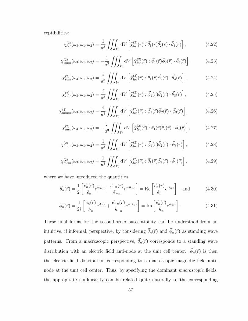
ceptibilities:
χ(2)eee(ω3;ω1, ω2) =
1
a3
∫∫∫V0
dV[
¯χ(2)loc(~r) : ~θ1(~r)~θ2(~r) · ~θ3(~r)
], (4.22)
χ(2)emm(ω3;ω1, ω2) = − 1
a3
∫∫∫V0
dV[
¯χ(2)loc(~r) : ~φ1(~r)~φ2(~r) · ~θ3(~r)
], (4.23)
χ(2)eem(ω3;ω1, ω2) =
i
a3
∫∫∫V0
dV[
¯χ(2)loc(~r) : ~θ1(~r)~φ2(~r) · ~θ3(~r)
], (4.24)
χ(2)eme(ω3;ω1, ω2) =
i
a3
∫∫∫V0
dV[
¯χ(2)loc(~r) : ~φ1(~r)~θ2(~r) · ~θ3(~r)
], (4.25)
χ(2)mmm(ω3;ω1, ω2) =
i
a3
∫∫∫V0
dV[
¯χ(2)loc(~r) : ~φ1(~r)~φ2(~r) · ~φ3(~r)
], (4.26)
χ(2)mee(ω3;ω1, ω2) = − i
a3
∫∫∫V0
dV[
¯χ(2)loc(~r) : ~θ1(~r)~θ2(~r) · ~φ3(~r)
], (4.27)
χ(2)mme(ω3;ω1, ω2) =
1
a3
∫∫∫V0
dV[
¯χ(2)loc(~r) : ~φ1(~r)~θ2(~r) · ~φ3(~r)
], (4.28)
χ(2)mem(ω3;ω1, ω2) =
1
a3
∫∫∫V0
dV[
¯χ(2)loc(~r) : ~θ1(~r)~φ2(~r) · ~φ3(~r)
], (4.29)
where we have introduced the quantities
~θn(~r) =1
2
[~en(~r)
eneiknz +
~e−n(~r)
e−ne−iknz
]= Re
[~en(~r)
eneiknz
]and (4.30)
~φn(~r) =1
2i
[~en(~r)
hneiknz +
~e−n(~r)
h−ne−iknz
]= Im
[~en(~r)
hneiknz
]. (4.31)
These final forms for the second-order susceptibility can be understood from an
intuitive, if informal, perspective, by considering ~θn(~r) and ~φn(~r) as standing wave
patterns. From a macroscopic perspective, ~θn(~r) corresponds to a standing wave
distribution with an electric field anti-node at the unit cell center. ~φn(~r) is then
the electric field distribution corresponding to a macroscopic magnetic field anti-
node at the unit cell center. Thus, by specifying the dominant macroscopic fields,
the appropriate nonlinearity can be related quite naturally to the corresponding
57

microscopic fields. In this way, the macroscopic field symmetries are enforced in the
local response, such that the homogenized nonlinearities are unambiguous. As an
example, typical plots of ~θ(~r) and ~φ(~r) are shown in Fig. 4.1 for a MM consisting of
high-dielectric spheres, obtained from eigenfrequency simulations.
Figure 4.1: (Reproduced with permission from Ref. [82]. Copyright (2012) bythe American Physical Society.) (a) The unit cell of an example MM composed of
high-dielectric spheres, illustrating the coordinate (~r) and lattice (~R) vectors. (b)
and (c) represent typical cross-sections of ~θ(~r) and ~φ(~r), respectively, obtained fromeigenfrequency simulations for spheres with ε/ε0 = 300 and diameter a/3 embeddedin free-space, showing the expected electric and magnetic-type responses.
This final result for the effective second-order magnetoelectric susceptibilities is
very satisfying and highly intuitive. By rearranging the Bloch modes, we are able to
describe the local electric fields that are, from a macroscopic perspective, either elec-
trically or magnetically induced. The effective response is completely characterized
by the overlap of these local field distributions within the nonlinear component of the
unit cell. In short, Eqs. (4.22) through (4.29) reveal that, as expected, clever struc-
turing of MM inclusions can give rise to complex macroscopic nonlinear behaviors of
a fundamentally different nature than the constituents.
The above analysis assumed propagation along the z-axis for simplicity, as well as
a homogenized medium whose normal modes, in the linear regime, are linearly polar-
ized plane waves. Thus, while the effective nonlinear susceptibilities are themselves
58

tensors, the above procedure only probes a single element of each tensor, determined
by the polarizations of the macroscopic waves, i.e. the χ(2)eee in the above formalism
is actually χ(2)eee,xxx, χ
(2)mmm is χ
(2)mmm,yyy, etc. However, even if the local nonlinearity is
diagonal, the subwavelength structure of the MM can give rise to overlap between the
different polarizations and thus non-zero cross-terms in the effective tensors [59, 83].
To recover the other elements of the susceptibility tensors, the polarization and direc-
tion of each wave can be manipulated successively, and the above procedure repeated
independently for each tensor element. Additionally, if the normal modes of the lin-
ear homogenized medium cannot be decomposed into linearly polarized plane waves,
as is the case, for example, in chiral MMs, an appropriate basis for homogenization,
with well-defined wave impedances and wavevectors, should be used instead.
We note here that the decision to write the equations of motion for the fields at ω3
is an arbitrary one. However, certain permutation symmetries and self-consistencies
are readily found in the above expressions. Assuming ω3 > ω2 > ω1 > 0, permutation
of the fundamental waves gives the same effective nonlinearity, i.e. χ(2)eme(ω3;ω1, ω2) =
χ(2)eem(ω3;ω2, ω1). Additionally, the complimentary nonlinearities, by which we mean
the nonlinearities describing the three-wave mixing process at the fundamental fre-
quencies, are the conjugate of the first, i.e. χ(2)eme(ω3;ω1, ω2) =
[χ
(2)mee(ω1;ω3,−ω2)
]∗=[
χ(2)eem(ω2;ω3,−ω1)
]∗, where we have used the constraint of real total fields to relate
the negative and positive frequency components. These properties of the nonlinear
susceptibilities can be shown to ensure the proper photon and energy conservation
requirements, as in the Manley-Rowe relations [49].
Finally, it is also worth noting that the units of the second-order susceptibilities
are not all the same, but have been chosen to ensure the permutation symmetries
discussed above. As seen in Eq. (4.3), each nonlinear susceptibility enters the equa-
tion for the coupling coefficient with a different leading coefficient, related to the
59

wave impedances at the involved frequencies. Using Eq. (4.18), it is convenient to
define individual coupling coefficients,
γg3g1g2 = ω3
√G1G2G3χ
(2)g3g1g2
(4.32)
where Gn = Zn for gn = e, and Gn = Yn = 1/Zn for gn = m, such that
Γν,ρ,ψ = γ(2)eee + sgn(ρ)γ(2)
eme + sgn(ψ)γ(2)eem + sgn(ρψ)γ(2)
emm
+ sgn(ν)γ(2)mee + sgn(ρν)γ(2)
mme + sgn(ψν)γ(2)mem + sgn(ρψν)γ(2)
mmm, (4.33)
where sgn() is the signum function. The eight individual coupling coefficients have
units of m−1(W/m2)−1/2, and provide a means for direct comparison of the relative
magnitudes and phases of the various second-order susceptibilities. Also, it is worth
noting that the contributions from each nonlinearity to Γν,ρ,ψ are uniquely dependent
on the propagation directions of the three waves, denoted in our convention by the
sign of the subscripts: a fact responsible for interesting interference effects in the
presence of multiple nonlinearities, as discussed in Section 4.3.1.
60

4.1.3 The effective third-order susceptibilities
Analogous to the second-order material responses of Eqs. (2.17) and (2.18), let us
consider a third-order polarization and magnetization of the form
~P (3)(t) =∑pqr
[¯χ(3)eeee(ωs;ωp, ωq, ωr)
... ~E(ωp) ~E(ωq) ~E(ωr)
+ ¯χ(3)eemm(ωs;ωp, ωq, ωr)
... ~E(ωp) ~H(ωq) ~H(ωr) + ¯χ(3)eeem(ωs;ωp, ωq, ωr)
... ~E(ωp) ~E(ωq) ~H(ωr)
+ ¯χ(3)eeme(ωs;ωp, ωq, ωr)
... ~E(ωp) ~H(ωq) ~E(ωr) + ¯χ(3)emee(ωs;ωp, ωq, ωr)
... ~H(ωp) ~E(ωq) ~E(ωr)
+ ¯χ(3)emmm(ωs;ωpωq, ωr)
... ~H(ωp) ~H(ωq) ~H(ωr) + ¯χ(3)emem(ωs;ωp, ωq, ωr)
... ~H(ωp) ~E(ωq) ~H(ωr)
+ ¯χ(3)emme(ωs;ωp, ωq, ωr)
... ~H(ωp) ~H(ωq) ~E(ωr)
]exp(−iωst), (4.34)
µ0~M (3)(t) =
∑pqr
[¯χ(3)mmmm(ωs;ωp, ωq, ωr)
... ~H(ωp) ~H(ωq) ~H(ωr)
+ ¯χ(3)mmee(ωs;ωp, ωq, ωr)
... ~H(ωp) ~E(ωq) ~E(ωr) + ¯χ(3)mmme(ωs;ωp, ωq, ωr)
... ~H(ωp) ~H(ωq) ~E(ωr)
+ ¯χ(3)mmem(ωs;ωp, ωq, ωr)
... ~H(ωp) ~E(ωq) ~H(ωr) + ¯χ(3)memm(ωs;ωp, ωq, ωr)
... ~E(ωp) ~H(ωq) ~H(ωr)
+ ¯χ(3)meee(ωs;ωp, ωq, ωr)
... ~E(ωp) ~E(ωq) ~E(ωr) + ¯χ(3)meme(ωs;ωp, ωq, ωr)
... ~E(ωp) ~H(ωq) ~E(ωr)
+ ¯χ(3)meem(ωs;ωp, ωq, ωr)
... ~E(ωp) ~E(ωq) ~H(ωr)
]exp(−iωst), (4.35)
where∑
pqr denotes a triple sum and ωs = ωp +ωq +ωr, thus defining 16 third-order
susceptibility tensors of rank 4. The same procedure as in the previous section can be
carried out for four-wave mixing in a MM composed of a periodic electric third-order
susceptibility, ¯χ(3)loc(~r). This gives a system of 16 equations relating the microscopic
61

Bloch field distributions to the 16 macroscopic susceptibilities, represented by
1
a3
∫∫∫V0
dV
(¯χ
(3)loc(~r)
...~eρ(~r)~eψ(~r)~eζ(~r) · ~e∗ν(~r))
=
χ(3)eeeeeρeψeζ eν + χ(3)
eemeeρhψeζ eν + χ(3)eeemeρeψhζ eν + χ(3)
eemmeρhψhζ eν
+ χ(3)meeeeρeψeζ hν + χ(3)
memeeρhψeζ hν + χ(3)meemeρeψhζ hν + χ(3)
memmeρhψhζ hν
+ χ(3)emeehρeψeζ eν + χ(3)
emmehρhψeζ eν + χ(3)ememhρeψhζ eν + χ(3)
emmmhρhψhζ eν
+ χ(3)mmeehρeψeζ hν + χ(3)
mmmehρhψeζ hν + χ(3)mmemhρeψhζ hν + χ(3)
mmmmhρhψhζ hν ,(4.36)
for ρ = ±1, ψ = ±2, ζ = ±3, ν = ±4. As before, assuming lossless materials, 16
closed form expressions can be derived for the effective third-order susceptibilities of
the form
χ(3)eeme(ω4;ω1, ω2, ω3) =
i
a3
∫∫∫V0
dV
[¯χ
(3)loc(~r)
...~θ1(~r)~φ2(~r)~θ3(~r) · ~θ4(~r)
]. (4.37)
For brevity, and due to similarities with the second-order expressions, we will omit
the equations for the 15 other third-order susceptibilities.
4.2 Numerical examples
According to (4.22) through (4.29), the eight homogenized nonlinear magnetoelectric
susceptibilities can be evaluated directly from the Bloch modes at the three frequen-
cies, found either analytically or numerically. Moreover, since the quantities in the
denominators of (4.30) and (4.31) are explicitly derived from the numerators, the
phases and amplitudes of ~θn(~r) and ~φn(~r) are automatically normalized, precluding
the usual problems associated with ill-defined Bloch modes. When calculating the
effective nonlinearities from numerical simulations, the computed Bloch modes can
be used directly in (4.30) and (4.31), facilitating the homogenization process. Thus,
the effective linear and nonlinear properties describing three-wave mixing in a MM
62

can be characterized from the results of just three eigenfrequency simulations. In this
section, we apply this procedure to several example MMs, demonstrating the ability
of these structures to support electric, magnetic, and magnetoelectric second-order
responses.
4.2.1 The split ring resonator
In order to validate the above expressions for the second-order susceptibilities, we
first apply the analysis to a well-researched nonlinear MM: the split-ring resonator
(SRR). For simplicity, we assume the local second-order response of the SRR is zero
everywhere except for a small dielectric slab loaded into the structure’s capacitive
gap, modeled by ε/ε0 = 25 and χ(2)loc,zzz/ε0 = 1pm/V. The background dielectric is
taken to be that of free-space. To allow extrapolation over a wide range of frequen-
cies, the SRR’s dimensions, given in Fig. 4.2 (a), are related to the lattice constant
a, and the results are given as a function of normalized frequencies, ωna/2πc. To
validate the use of Eq. (4.21), dielectric losses are neglected, and the metal ring
is modeled by a perfect electric conductor with thickness a/100. Using COMSOL
Multiphysics, we employ eigenfrequency simulations on the unit cell to determine
the lowest forward propagating Bloch modes and eigenfrequencies over a range of
wavevectors, assuming the incident fields are polarized according to Fig. 4.2 (a). In
this way, we first determine the wavevectors and wave impedances as a function of
frequency, according to Ref. [12]. From previous theoretical investigations [74], we
know that, when excited by a fundamental frequency (FF) close to the magnetic res-
onance, SHG is mediated by the purely magnetic nonlinearity, χ(2)mmm. Moreover, due
to the small size and high permittivity of the nonlinear dielectric, the z component
of the electric field within the gap is nearly constant, allowing the integral in Eq.
(4.26) to be approximated by the product of the average values of ~φn within the gap
and the nonlinear dielectric’s volume. Thus, we record the eigenfrequency and ~φn · z
63

in the gap for a wide range of wavevectors, interpolating the results to determine
χ(2)mmm(2ω;ω, ω) as a function of the normalized FF ωa/2πc, according to Eq. (4.26).
Figure 4.2: (Reproduced with permission from Ref. [82]. Copyright (2012) by theAmerican Physical Society.) (a) Nonlinear SRR used in validating Eq. (4.26). Plotsof the SRR’s retrieved linear (b) and nonlinear (c) properties via both scattering
and eigenfrequency simulations. The effective χ(2)mmm(2ω;ω, ω) is retrieved by both
the nonlinear transfer matrix method and Eq. (4.26), showing excellent agreement.The grayed frequency bands where no data is plotted correspond to either the FF orsecond-harmonic falling in the SRR’s stop band that extends over a narrow range offrequencies above the magnetic resonance.
For comparison, we perform full-wave numerical simulations, using the exist-
ing nonlinear parameter retrieval method based on transfer matrices [67, 70]. This
method has been previously established for the retrieval of purely magnetic nonlinear-
ities [69, 84]. Thus, we retrieve the effective magnetic nonlinearity, χ(2)mmm(2ω;ω, ω),
from nonlinear scattering simulations for a single unit cell with appropriate periodic
boundary conditions. The linear properties are likewise determined from the linear
scattering parameters [11]. The results of both retrieval techniques are presented in
Fig. 4.2 (b) and (c). The excellent agreement between the two methods lends valid-
ity to the procedure employed here. Small discrepancies between the two approaches
can be attributed to the coupling between neighboring unit cells in the direction of
propagation, neglected in the scattering simulations.
64

4.2.2 Prototypical nonlinear magnetoelectric metamaterial
Recently, nonlinear magnetoelectric coupling was demonstrated in a MM at mi-
crowave frequencies [76]. The MMs were varactor loaded split-ring resonators (VL-
SRRs), consisting of copper ring resonators with two capacitive gaps on either side.
The varactor diodes provided the second-order response. Unlike the previous SRR,
the gaps were oriented such that both electric and magnetic fields could excite volt-
ages across the varactors, allowing nonlinear magnetoelectric coupling to take place.
Here, we analyze the analogous doubly-split ring resonator depicted in Fig. 4.3
(a), in which the capacitive gaps are loaded with small nonlinear dielectric films, as in
the previous example. The effective linear properties are obtained via field averaging
and plotted in Fig. 4.3 (b), showing the expected magnetic resonance. In terms of the
nonlinear properties, we consider two structures, corresponding to orientation of the
nonlinear dielectrics in the same direction (symmetric SRR), or in opposite directions
(anti-symmetric SRR). These configurations imply even and odd symmetries in the
nonlinear properties with respect to the z-coordinate, i.e. ¯χ(2)loc(x, y, z) = ¯χ
(2)loc(x, y,−z)
and ¯χ(2)loc(x, y, z) = − ¯χ
(2)loc(x, y,−z), respectively. We follow the same procedure as
before, but evaluating all of the second-order susceptibilities for both configurations.
The magnitudes of the strongest four γ are plotted in Fig. 4.3 (c) and (d), normalized
by the value for a solid block of the nonlinear dielectric, γloc.
At the resonance frequency, we see the dominant nonlinear process to be
χ(2)mmm(2ω;ω, ω) in the anti-symmetric SRR, and χ
(2)emm(2ω;ω, ω) in the symmetric
SRR, in agreement with experiments on analogous VLSRRs [76]. The nature of
these differing nonlinearities is further illustrated in Fig. 4.3 (e) and (f), which give
a cross-section of the SHG electric fields outside of the MM. These SHG field maps
are generated from an infinite column of SRRs resonantly excited by a FF plane wave
with the indicated polarization and direction. The electric- and magnetic-dipole-like
65

Figure 4.3: (Reproduced with permission from Ref. [82]. Copyright (2012) by theAmerican Physical Society.) (a) The doubly-split nonlinear SRR used for both thesymmetric and anti-symmetric configurations. (b) The retrieved linear propertiesfrom eigenfrequency simulations. The second-order susceptibilities of the symmetric(c) and anti-symmetric (d) SRRs for SHG, calculated via (4.22) through (4.29). Due
to the degenerate frequencies involved in SHG, χ(2)eem and χ
(2)eme are identical, as are
χ(2)mem and χ
(2)mme. (e) and (f) show field maps of resonant SHG from infinite columns
of symmetric and anti-symmetric SRRs, respectively.
patterns are clearly evident in the SHG radiation patterns.
These plots display a number of other prominent features. In particular, the
contrasting symmetries in the nonlinear properties of the two unit cells result in two
distinct sets of nonlinear susceptibilities. The susceptibilities are highly dispersive,
with different nonlinearities dominant at different frequencies. On the one hand,
since the magnetic induction of the SRR must go to zero as the frequencies go to
DC, we see that all of the nonlinearities vanish in this limit, with the exception of
χ(2)eee, which flattens out to a constant value nearly equal to the nonlinear dielectric
alone. This non-resonant enhancement of the electric nonlinearity is impressive when
considering that the nonlinear dielectric makes up less than 1 part in 50,000 of the
MM’s volume. On the other hand, when one of the involved frequencies is tuned
66

near the magnetic resonance frequency, we see that the overall nonlinear activity of
the MM exceeds that of the nonlinear dielectric by orders of magnitude.
4.3 Examples of nonlinear magnetoelectric phenomena
Up until now, we have focused on the problem of constructing and characterizing
nonlinear magnetoelectric MMs, but avoided discussing how the full set of nonlinear
susceptibilities can be used to achieve unique and interesting phenomena. Indeed,
the parameter space that Eqs. (4.22) through (4.29) encompass is gigantic, espe-
cially when the tensorial nature of the nonlinear susceptibilities is considered. While
it is beyond the scope of this paper to search out and categorize the range of phe-
nomena nonlinear magnetoelectric MMs can give rise to, this section is devoted to
two demonstrative examples. First, we consider interference effects in MMs possess-
ing two nonlinear susceptibilities of comparable magnitude. Having direct analogues
in natural materials, nonlinear interference effectively tailors the harmonic and mix
wave generation by suppressing and/or enhancing generation along certain direc-
tions, especially in optically thin slabs. Second, we analyze electro-optic effects in
such MMs under the application of a static electric field. We show that, depending
on geometry, the linear permittivity, permeability, and/or magnetoelectric coupling
coefficient can be tuned by applying a voltage to the bulk MM. These examples are
further illustrated through the prototypical SRRs of Section 4.2.2.
4.3.1 Nonlinear interference
From Fig. 4.3, it is clear certain MM designs can support nonlinear processes with
contributions from several effective nonlinear susceptibilities. The fields generated by
the different nonlinearities can potentially interfere with each other, either enhancing
or suppressing harmonic and mix wave generation. Nonlinear interference has been
demonstrated in certain antiferromagnetic compounds [85, 86, 87], for example, in
67

which χ(2)eee and χ
(2)mee are found to have similar magnitudes. The process, however,
is generally very weak and has been used mostly in probing the antiferromagnetic
domains in such materials, using the fact that χ(2)eee reverses sign when going from
one domain to another [88].
To offer a concrete example of nonlinear interference, let us consider collinear DFG
in a homogeneous (or homogenized) medium, wherein forward propagating waves at
ω3 and ω2 generate forward and backward waves at the frequency ω1 = ω3 − ω2. If
we assume a sufficiently weak nonlinearity, we can take A3 and A2 to be constant,
known as the non-depleted pump approximation. Assuming a slab of length L and
no initial input at ω1, Eq. (4.2) can be solved to give the intensities of the forward
and backward DFG waves,
I1(z) =1
2I3I2|Γ1,3,2∗ |2sinc2
((k3 − k2 − k1)
z
2
)z2, (4.38)
I−1(z) =1
2I3I2|Γ−1,3,2∗|2sinc2
((k3 − k2 + k1)
L− z2
)(L− z)2, (4.39)
where, since we are considering DFG, the notation 2∗ is used to indicate a negative
frequency in calculating the coupling coefficient. Nonlinear interference, then, refers
to the fact that the coupling coefficients in Eqs. (4.38) and (4.39) are superpositions
of the eight second-order susceptibilities, which can add constructively or destruc-
tively in the generation of the forward and backward waves, A±1, depending on the
relative phases and magnitudes of the susceptibilities, as well as the directionality of
the involved waves. That is to say, |Γ1,3,2| is not necessarily equal to |Γ−1,3,2|. Alter-
natively, if only one nonlinearity is dominant, it is easy to verify that the magnitudes
of the coupling coefficients are independent of inversion of any of the involved waves,
or inversion of the medium itself.
While it may seem difficult and coincidental to find a MM supporting two second-
order susceptibilities with similar enough magnitudes to make this effect noticeable,
68

the permutation symmetries detailed above can lead to this behavior quite naturally.
For example, let us consider DFG in the symmetric doubly-split ring resonator MM,
or χ(2)(ω1;ω3,−ω2) for ω3 > ω1,2. In particular, we take ω3a/2πc = 0.087, close
to the resonance frequency, while sweeping the other frequencies and calculate the
associated nonlinearities, shown in Fig. 4.4. Permutation symmetry implies that
χ(2)emm(ω1;ω3,−ω2) → χ
(2)mme(ω1;ω3,−ω2) in the limit that ω1 ≈ ω2 ≈ ω3/2, resulting
in the crossing point in Fig. 4.4 (a). Since these are the dominant nonlinearities
contributing to DFG, we see from Eq. (4.33) that Γ1,3,2∗ ≈ 2γemm and Γ−1,3,2∗ ≈ 0 in
the limit ω1 → ω2 → ω3/2, leading to unidirectional DFG in the forward direction.
Figure 4.4: (Reproduced with permission from Ref. [82]. Copyright (2012) bythe American Physical Society.) The second-order susceptibilities of the symmetric(a) and anti-symmetric (b) SRRs for DFG, calculated via (4.22) through (4.29), forω3a/2πc = 0.087. (c) and (d) show field maps of DFG from infinite columns of sym-metric and anti-symmetric SRRs, respectively, in the nearly degenerate case. Thecomparable magnitudes in the two dominant nonlinear susceptibilities leads to uni-directional DFG, favoring forward generation in the symmetric SRR, and backwardgeneration in the anti-symmetric SRR.
For the same configuration, DFG in the anti-symmetric SRR is dominated by
69

both χ(2)mmm and χ
(2)eme, owing to a rough balance of the electric and magnetic coupling
strengths at these frequencies, as shown in Fig. 4.4 (b). However, these nonlinear
susceptibilities are out of phase, in contrast to the previous example. The result
is that forward DFG is suppressed, in favor of backward DFG. Such unidirectional
behavior is fundamentally different from that associated with phase matching, and
is in fact most noticeable in subwavelength slabs where phase matching effects are
negligible. Indeed, interference between nonlinear magnetoelectric susceptibilities
offers an alternate route towards realizing unidirectional devices such as the nonlinear
optical mirror [89]. The unidirectional behavior is further illustrated in the field maps
shown in Fig. 4.4 (c) and (d). Similar to Fig. 4.3, the field maps show a cross-section
of the DFG emanating from an infinite column of SRRs. The SRRs are excited by
plane waves at the resonance frequency and half the resonance frequency, so that the
DFG processes depicted in Fig. 4.4 (c) and (d) correspond to the mid-points of plots
(a) and (b), respectively, where the nonlinear interference is maximized.
4.3.2 Electro-optic effects
The tuning of optical properties is a highly desirable feature for many applications,
and no less so in magnetoelectric media [90]. Since the metamaterials considered
here have constituents that are susceptible to the electro-optic effect, it is natural
to consider what effect a static electric field can have on all of the metamaterial’s
effective properties, as described by the effective second-order susceptibilities. Thus,
let us consider the propagation of a monochromatic wave, labeled ‘s’, under the
application of a static electric field, labeled ‘0’. Under these conditions, we can show
70

that the corresponding second-order susceptibilities are given by
χ(2)eee(ωs; 0, ωs) =
1
a3
∫∫∫V0
dV[
¯χ(2)loc(~r) : ~θ0(~r)~θs(~r) · ~θs(~r)
], (4.40)
χ(2)mem(ωs; 0, ωs) =
1
a3
∫∫∫V0
dV[
¯χ(2)loc(~r) : ~θ0(~r)~φs(~r) · ~φs(~r)
], (4.41)
χ(2)eem(ωs; 0, ωs) =
i
a3
∫∫∫V0
dV[
¯χ(2)loc(~r) : ~θ0(~r)~φs(~r) · ~θs(~r)
], (4.42)
χ(2)mee(ωs; 0, ωs) = − i
a3
∫∫∫V0
dV[
¯χ(2)loc(~r) : ~θ0(~r)~θs(~r) · ~φs(~r)
], (4.43)
while all other nonlinearities must be identically zero. If we define the material
relations according to
~D(ω) = ¯ε ~E(ω) + i¯κ ~H(ω), (4.44)
~B(ω) = ¯µ ~H(ω)− i¯κ∗ ~E(ω), (4.45)
it follows that the effective material properties are given by
¯ε(ω, ~E0) = ε0
[1 + ¯χ(1)
ee (ω) +1
ε0¯χ(2)eee(ω; 0, ω) : ~E0
], (4.46)
¯µ(ω, ~E0) = µ0
[1 + ¯χ(1)
mm(ω) +1
µ0
¯χ(2)mem(ω; 0, ω) : ~E0
], (4.47)
¯κ(ω, ~E0) =1
c
[¯χ(1)em(ω) +
c
i¯χ(2)eem(ω; 0, ω) : ~E0
]. (4.48)
In this context, it appears quite natural that χ(2)eem and χ
(2)mee are purely imaginary for
transparent media, such that the effective linear magnetoelectric coupling coefficients
are real-valued.
In essence, Eqs. (4.46) through (4.48) constitute the electro-optic effect for the
linear electric, magnetic, and magnetoelectric properties, respectively. The corre-
sponding second-order susceptibilities for the two MMs are shown in Fig. 4.5, ap-
proximating ~θ0(~r) by a Bloch mode calculated at very low frequency. Thus, the
71

Figure 4.5: (Reproduced with permission from Ref. [82]. Copyright (2012) bythe American Physical Society.) The effective second-order susceptibilities of thesymmetric (b) and anti-symmetric (c) SRRs under a static electric field, calculatedvia (4.40) through (4.43).
symmetric SRR supports field-induced contributions to the permittivity and perme-
ability. The anti-symmetric SRR, on the other-hand, supports field-induced magne-
toelectric coupling. This is made particularly more interesting since magnetoelectric
coupling in this SRR vanishes in the absence of an electric field. Similar control
of optical activity has been realized in a chiral metamaterial through a third-order
nonlinear process [91]. In this way, the linear magnetoelectric properties of a medium
can be tuned dynamically.
4.4 Spatial dispersion in the nonlinear susceptibilities
As stated earlier, the expressions for the second-order nonlinearities in (4.22)-(4.29)
are only valid in the limit that a → 0. In other words, they neglect the spatial
72
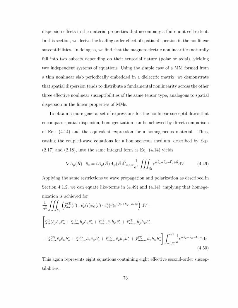
dispersion effects in the material properties that accompany a finite unit cell extent.
In this section, we derive the leading order effect of spatial dispersion in the nonlinear
susceptibilities. In doing so, we find that the magnetoelectric nonlinearities naturally
fall into two subsets depending on their tensorial nature (polar or axial), yielding
two independent systems of equations. Using the simple case of a MM formed from
a thin nonlinear slab periodically embedded in a dielectric matrix, we demonstrate
that spatial dispersion tends to distribute a fundamental nonlinearity across the other
three effective nonlinear susceptibilities of the same tensor type, analogous to spatial
dispersion in the linear properties of MMs.
To obtain a more general set of expressions for the nonlinear susceptibilities that
encompass spatial dispersion, homogenization can be achieved by direct comparison
of Eq. (4.14) and the equivalent expression for a homogeneous material. Thus,
casting the coupled-wave equations for a homogeneous medium, described by Eqs.
(2.17) and (2.18), into the same integral form as Eq. (4.14) yields
∇Aµ(~R) · sµ = iAρ(~R)Aψ(~R)Γµ,ρ,ψ1
a3
∫∫∫V0
ei(~kρ+~kψ−~kµ)·~RdV. (4.49)
Applying the same restrictions to wave propagation and polarization as described in
Section 4.1.2, we can equate like-terms in (4.49) and (4.14), implying that homoge-
nization is achieved for
1
a3
∫∫∫V0
(¯χ
(2)loc(~r) : ~eρ(~r)~eψ(~r) · ~e∗ν(~r)ei(kρ+kψ−kν)z
)dV =
[¯χ(2)eeeeρeψe
∗ν + ¯χ(2)
emehρeψe∗ν + ¯χ(2)
eemeρhψe∗ν + ¯χ(2)
emmhρhψe∗ν
+ ¯χ(2)meeeρeψh
∗ν + ¯χ(2)
mmehρeψh∗ν + ¯χ(2)
memeρhψh∗ν + ¯χ(2)
mmmhρhψh∗ν
] ∫ a/2
−a/2
1
aei(kρ+kψ−kν)zdz.
(4.50)
This again represents eight equations containing eight effective second-order suscep-
tibilities.
73

By comparing Eq. (4.50) to (4.20), we see that the approximation inherent in
Section 4.1.2 is equivalent to∫ a/2−a/2
1aei(kρ+kψ−kν)z′dz′ ≈ 1, i.e., the phase mismatch
accumulated over a single unit cell is small. This is not always valid, as many MM
unit cells have lattice constants that are not entirely negligible in comparison to the
wavelength. As such, the previous steps cannot be repeated to yield a closed form
expression for each nonlinear susceptibility. For example, if we attempt to derive an
expression analogous to (4.22), we find
1
a2
∫∫∫V0
[¯χ
(2)loc(~r) : ~θ1(~r)~θ2(~r) · ~θ3(~r)
]dV =
χ(2)eee
∫ a/2
−a/2cos(k1z) cos(k2z) cos(k3z)dz
+ iχ(2)eme
h1
e1
∫ a/2
−a/2sin(k1z) cos(k2z) cos(k3z)dz
+ iχ(2)eem
h2
e2
∫ a/2
−a/2cos(k1z) sin(k2z) cos(k3z)dz
− χ(2)emm
h1h2
e1e2
∫ a/2
−a/2sin(k1z) sin(k2z) cos(k3z)dz
− iχ(2)mee
h3
e3
∫ a/2
−a/2cos(k1z) cos(k2z) sin(k3z)dz
+ χ(2)mme
h1h3
e1e3
∫ a/2
−a/2sin(k1z) cos(k2z) sin(k3z)dz
+ χ(2)mem
h2h3
e2e3
∫ a/2
−a/2cos(k1z) sin(k2z) sin(k3z)dz
+ iχ(2)mmm
h1h2h3
e1e2e3
∫ a/2
−a/2sin(k1z) sin(k2z) sin(k3z)dz. (4.51)
Rather than a single effective nonlinear susceptibility, the right-hand side appears
to contain contributions from all eight. However, since the limits of the integrals
74

on the right-hand side of Eq. (4.51) are symmetric, all of the terms containing odd
integrands, or equivalently an odd number of sine terms, must vanish, leaving just
four non-zero terms. This procedure can be repeated to find all eight analogous
equations (see Appendix 4.7). In doing so, the nonlinear susceptibilities naturally
fall into two subsets, such that all of the terms from one subset or the other vanish
in any given matrix element, leading to two independent systems of equations. The
reason for this separation can be understood by considering the effective nonlinear
tensor types. Specifically, for the construction considered here, the effective nonlin-
earities ¯χ(2)eee, ¯χ
(2)mme, ¯χ
(2)mem, and ¯χ
(2)emm are polar tensors, while ¯χ
(2)mmm, ¯χ
(2)eem, ¯χ
(2)eme, and
¯χ(2)mee are axial tensors. This follows naturally from the polar and axial vector nature
of the electric and magnetic fields themselves, and the assumption that the local
nonlinearity is a polar tensor [92]. Since spatial dispersion in this context should
not depend on the handed-ness of the coordinate system, it follows that the affected
susceptibilities must be of the same tensor type.
Figure 4.6: (Reproduced with permission from Ref. [82]. Copyright (2012) by theAmerican Physical Society.) (a) Illustration of the unit cell for investigating spatialdispersion in the nonlinear properties, consisting of a thin nonlinear slab of thicknessd embedded in a dielectric matrix with periodicity a. (b) The effective nonlinear
susceptibilities, assuming εr = 2, d/a = 0.01, χ(2)loc/ε0 = 100 pm/V, ω2 = 1.5ω1, and
ω3 = ω1 + ω2, as a function of ω3a/2πc.
75

To see how a non-negligible unit cell extent changes the effective nonlinear prop-
erties of a MM, let us use the example of a 1-dimensional MM consisting of a thin
nonlinear dielectric slab of extent d, periodically loaded in a dielectric spacer with
period a, shown in Fig. 4.6. For propagation normal to the slab, the field and po-
larization vectors become scalar. Moreover, to remove the effects of linear spatial
dispersion, let us assume the slab and dielectric spacer have the same relative per-
mittivity, εr. Thus, the Bloch modes are simple plane waves with kn =√εrωn/c. In
the long-wavelength limit, Eqs. (4.22) through (4.29) reveal that all of the effective
nonlinear susceptibilities vanish except for the electric nonlinearity, which reduces to
a simple volume average of the local nonlinearity,
χ(2)eee(ω3;ω1, ω2) =
d
aχ
(2)loc long wavelength limit, (4.52)
in agreement with previous studies of composite nonlinear media [59]. Since the non-
linear susceptibilities naturally separate into two subsets, the four c-type nonlinear
susceptibilities are identically zero for all wavelengths. This leaves us with a system
of four equations and four unknown i-type nonlinear susceptibilities. If d = a, i.e.
the medium is simply a homogeneous slab of nonlinear dielectric, then (4.57)-(4.64)
can be solved to give χ(2)eee = χ
(2)loc for all frequencies, as expected. On the other hand,
in the limit d << a, the left-hand sides of (4.58)-(4.64) vanish. Solving this system
to leading order in kia, we find
χ(2)eee =
[1− 1
8a2(k2
1 + k22 + k2
3
)] daχ
(2)loc (4.53)
χ(2)emm = +Z1Z2
(1
12a2k1k2
)d
aχ
(2)loc = +Z2
0
(π2
3
a2
λ1λ2
)d
aχ
(2)loc (4.54)
χ(2)mme = −Z1Z3
(1
12a2k1k3
)d
aχ
(2)loc = −Z2
0
(π2
3
a2
λ1λ3
)d
aχ
(2)loc (4.55)
χ(2)mem = −Z2Z3
(1
12a2k2k3
)d
aχ
(2)loc = −Z2
0
(π2
3
a2
λ2λ3
)d
aχ
(2)loc (4.56)
76

where λn = 2πc/ωn is the wavelength in free-space. Thus, spatial dispersion mani-
fests itself in the susceptibilities of the same inversion symmetry, proportional to the
square of the lattice constant-to-wavelength ratio. The second-order susceptibilities
are plotted in Fig. 4.6 (b) for typical values. While the above equations are specific
to this example, the qualitative behavior and consequences of spatial dispersion in
the nonlinear properties can be considered representative of MMs in general.
4.5 Symmetry considerations
At this point, it is useful to consider the effective nonlinear properties from a sym-
metry standpoint. Given that the eight nonlinear tensors naturally separate into
polar and axial tensors, we would expect that the internal symmetries of a given
metamaterial would favor one group of tensors over another. For example, let us
consider a metamaterial whose linear properties are centrosymmetric, that is, for
some choice of origin ~ε(~r) = ~ε(−~r) for all ~r within the unit-cell. Such symmetry is
a good approximation for regular arrangements of nanoparticles and many circuit-
based metamaterials like dual-split SRRs and ELCs. It is worth noting that we
are not referring to the crystal symmetry of the local materials, at least some of
which must be non-centrosymmetric to support a χ(2)loc, but rather the structural
symmetry of the metamaterial unit-cell, which depends on the relative arrangement
of the constituent materials and inclusions. As such, even though the anisotropy of
the nonlinear elements, as well as the presence of substrates, will, strictly speaking,
break the inversion symmetry, it is instructive to consider the structural symmetry
of the inclusion as the dominant force influencing the effective properties. In any
case, for a centrosymmetric unit-cell, we know from Bloch theory that a similar sym-
metry is enforced in the local fields, or ~en(~r) = ~en(−~r)∗. From their definitions, we
see that this in turn implies that ~θ(~r) is an even function of ~r, while ~φ(~r) is odd.
77

Figure 4.7: Illustration of symmetries in nonlinear metamaterials. (a) A cen-trosymmetric inclusion, the double-gap SRR, placed over a uniform nonlinear sub-strate for maximizing the polar second-order susceptibility tensors. (b) A centrosym-metric inclusion placed over an anti-symmetric nonlinear substrate for maximizingthe axial second-order susceptibility tensors. (c) A non-centrosymmetric inclusionplaced over a uniform substrate excludes neither polar nor axial second-order sus-ceptibility tensors.
Clearly, these symmetry properties will have a strong impact on which effective non-
linearities are dominant. If the nonlinear properties are similarly centrosymmetric,
i.e. χ(2)loc(~r) = χ
(2)loc(−~r), then the integrands of the axial nonlinear tensors are odd
functions of ~r and therefore the axial nonlinear tensors vanish identically. If, on the
other hand, the material is poled in such a way that the local nonlinear properties
are anti-symmetric, χ(2)loc(~r) = −χ(2)
loc(−~r), then the polar nonlinear tensors vanish.
These cases are illustrated in Fig. 4.7 (a) and (b), respectively.
At microwave frequencies, where circuit elements such as varactor diodes are
often used as the nonlinear inclusions, it is simple to choose the symmetries in the
nonlinear properties, giving access to any of the eight nonlinear susceptibilities. At
optical frequencies, however, local electric nonlinearities are often introduced by using
a nonlinear crystal as a substrates or embedding matrix. While a nonlinear crystal
as a whole can be aligned along a particular axis, enforcing local directionality in a
bulk medium or substrate can be very difficult, especially on the length scales that
would be required in a metamaterial. This implies that, at optical frequencies, the
78

class of nonlinear metamaterials composed of centrosymmetric inclusions will tend
to support nonlinear processes through effectively polar nonlinear tensors. Accessing
the axial tensors requires non-centrosymmetric inclusions, such as the single-gap SRR
shown in Fig. 4.7 (c), which is known to support nonlinearites of the type χ(2)mmm [69].
4.6 Conclusion
Through a coupled-mode analysis, we have developed a method for describing the
nonlinear behavior of MMs in terms of well-known nonlinear susceptibilities. These
effective nonlinear susceptibilities are derived directly from the microscopic fields
supported by the MM, giving a physically intuitive perspective of the nonlinear prop-
erties. By investigating these relations analytically and numerically, we have shown
that the macroscopic nonlinear behavior of MMs can differ from its constituent ma-
terials not only in magnitude but in kind. In a simple dual-gap SRR medium, we
were able to demonstrate a configuration and frequency combination at which each
of the eight second-order susceptibilities, defined in Eqs. (2.17) and (2.18), was the
dominant nonlinearity. However, it is likely that more interesting and beneficial
structures can maximize the usefulness of nonlinear mangetoelectric coupling, par-
ticularly chiral MMs, owing to the prominent role magnetoelectric coupling plays in
such mediums.
To give context to this work, we note that certain magnetic materials are known to
support wave-mixing processes, such as SHG, mediated through naturally occurring
magnetoelectric nonlinearities [93, 94, 90, 95, 96]. These materials, however, are
rare, and the strengths of such processes are limited by the weak optical magnetic
responses of natural materials in general. In this context, the simple expressions in
(4.22)-(4.29) show that MMs can potentially support similar processes, but at far
higher efficiencies.
Perhaps most significantly, nonlinearities of different types can be brought to-
79

gether in a single medium in a controllable way that is simply impossible in naturally
occuring materials. This implies a virtually boundless design space for the nonlinear
properties of MMs. In particular, by combining nonlinear susceptibilities of roughly
equal magnitudes in a single medium, one can access the phenomena of nonlinear
interference, whereby unidirectional generation of harmonics and mix frequencies can
be achieved. Through clever design of the MM unit cell, nonlinear processes can be
suppressed to avoid parasitic losses, or enhanced by orders of magnitude to form the
core of compact, efficient nonlinear devices.
While we believe this work represents a fundamental step in understanding the
nonlinear magnetoelectric properties of MMs, it is by no means intended to be an
exhaustive description of the phenomena resulting from nonlinear magnetoelectric
coupling. Indeed, inspired by the wide range of potential applications that have
been found for various combinations of the linear electric, magnetic, and magne-
toelectric properties of MMs, we hope that this work will spark similar creativity
and ingenuity for combining the electric, magnetic, and magnetoelectric nonlinear
properties of MMs in new and unforeseen ways, while laying the foundations for the
design, characterization, and physics thereof.
80

4.7 Appendix: Derivation of the nonlinear susceptibilities in the pres-ence of spatial dispersion
Using the short-hand notation Sn = sin(knz) and Cn = cos(knz) and dropping the
explicit integral limits, we can rearrange (4.20) into the following eight equations:
1
a2
∫∫∫ [¯χ
(2)loc(~r) : ~θ1(~r)~θ2(~r) · ~θ3(~r)
]dV =
χ(2)eee
∫C1C2C3dz − χ(2)
emm
h1h2
e1e2
∫S1S2C3dz
+ χ(2)mem
h2h3
e2e3
∫C1S2S3dz + χ(2)
mme
h1h3
e1e3
∫S1C2S3dz, (4.57)
−1
a2
∫∫∫ [¯χ
(2)loc(~r) : ~φ1(~r)~φ2(~r) · ~θ3(~r)
]dV =
− χ(2)eee
e1e2
h1h2
∫S1S2C3dz + χ(2)
emm
∫C1C2C3dz
+ χ(2)mem
e1h3
h1e3
∫S1C2S3dz + χ(2)
mme
e2h3
h2e3
∫C1S2S3dz, (4.58)
1
a2
∫∫∫ [¯χ
(2)loc(~r) : ~θ1(~r)~φ2(~r) · ~φ3(~r)
]dV =
χ(2)eee
e2e3
h2h3
∫C1S2S3dz + χ(2)
emm
h1e3
e1h3
∫S1C2S3dz
+ χ(2)mem
∫C1C2C3dz − χ(2)
mme
h1e2
e1h2
∫S1S2C3dz, (4.59)
1
a2
∫∫∫ [¯χ
(2)loc(~r) : ~φ1(~r)~θ2(~r) · ~φ3(~r)
]dV =
χ(2)eee
e1e3
h1h3
∫S1C2S3dz + χ(2)
emm
h2e3
e2h3
∫C1S2S3dz
− χ(2)mem
e1h2
h1e2
∫S1S2C3dz + χ(2)
mme
∫C1C2C3dz, (4.60)
81

i
a2
∫∫∫ [¯χ
(2)loc(~r) : ~φ1(~r)~φ2(~r) · ~φ3(~r)
]dV =
χ(2)mmm
∫C1C2C3dz − χ(2)
mee
e1e2
h1h2
∫S1S2C3dz
+ χ(2)eme
e2e3
h2h3
∫C1S2S3dz + χ(2)
eem
e1e3
h1h3
∫S1C2S3dz, (4.61)
−ia2
∫∫∫ [¯χ
(2)loc(~r) : ~θ1(~r)~θ2(~r) · ~φ3(~r)
]dV =
− χ(2)mmm
h1h2
e1e2
∫S1S2C3dz + χ(2)
mee
∫C1C2C3dz
+ χ(2)eme
h1e3
e1h3
∫S1C2S3dz + χ(2)
eem
h2e3
e2h3
∫C1S2S3dz, (4.62)
i
a2
∫∫∫ [¯χ
(2)loc(~r) : ~φ1(~r)~θ2(~r) · ~θ3(~r)
]dV =
χ(2)mmm
h2h3
e2e3
∫C1S2S3dz + χ(2)
mee
e1h3
h1e3
∫S1C2S3dz
+ χ(2)eme
∫C1C2C3dz − χ(2)
eem
e1h2
h1e2
∫S1S2C3dz, (4.63)
i
a2
∫∫∫ [¯χ
(2)loc(~r) : ~θ1(~r)~φ2(~r) · ~θ3(~r)
]dV =
χ(2)mmm
h1h3
e1e3
∫S1C2S3dz + χ(2)
mee
e2h3
h2e3
∫C1S2S3dz
− χ(2)eme
h1e2
e1h2
∫S1S2C3dz + χ(2)
eem
∫C1C2C3dz. (4.64)
Eqs. (4.57) through (4.60) represent a system of four equations for the four polar
second-order susceptibility tensors, while Eqs. (4.61) through (4.64) represent an
independent system of four equations for the four axial second-order susceptibility
tensors. Both systems can be solved using linear algebra.
82

5
Engineering the effective nonlinear susceptibilities
Enhancing the otherwise weak optical nonlinearities associated with natural mate-
rials is one of the most enticing capabilities of NLMMs. Metamaterials naturally
support highly inhomogeneous field distributions, where electromagnetic energy can
be concentrated into small, critical volumes [2]. Any nonlinear element placed in
these volumes experiences a local field strength much greater than the average field.
Enhancement of nonlinearities through light localization is well known, and has been
exploited in plasmonic media [97, 98, 99, 100, 101], photonic crystals [102, 103], and
resonant cavities [104, 105]. However, there is a fundamental difference between the
field localization in these structures and that associated with NLMMs: cavities and
electromagnetic ‘hot spots’ localize fields to tiny spatial volumes, restricting configu-
rations to surfaces or similarly small fractions of the whole medium. Wave behavior
in such systems is typically described in terms of scattering rather than propaga-
tion, since the density and distribution of the enhancement regions are so sparse.
In contrast, the field localization in NLMMs is distributed periodically throughout
a volume with no fundamental constraint on wave propagation; in other words, the
enhancement associated with NLMMs is inherently a bulk effect, imbuing the meta-
83

material composite with an effective, continuous nonlinear susceptibility many times
greater than that of any of the constituent materials. This important distinction
renders NLMMs an approach to the design of a new generation of materials with
the potential for unprecedented bulk nonlinearities. Indeed, once designed, artificial
materials of this type can subsequently be used in many of these same advantageous
setups that are currently employed for natural materials, allowing for cumulative
mechanisms of enhancement. The following sections are reproduced with permission
from Alec Rose, Stephane Larouche, David R. Smith, Physical Review A, 84, 053805,
2011. Copyright (2011) by the American Physical Society.
5.1 The nonlinear retrieval method for media with nonlinear polar-ization and magnetization
The enhancement of nonlinear properties in NLMMs relates directly to the magni-
tude of the local field enhancement within the metamaterial elements. Full wave
simulations can offer direct measurements of the field enhancement factor by sim-
ulating the excitation of either metamaterial or plasmonic structures; however, the
results are specific to the setup employed, and do not constitute a general descrip-
tion of an effective medium comprising such structures. The ‘enhancement factors’
quoted in such studies are, at best, indirect measures of the resulting nonlinear prop-
erties [97, 98, 101]. Since it is our goal to demonstrate the enhancement of nonlinear
optical processes in a bulk NLMM medium, we require a tool for the accurate com-
putation of the NLMM’s effective nonlinear properties, using the results of nonlinear
scattering simulations on a single unit cell.
To apply the nonlinear retrieval method for the structures studied here, however,
some modifications are required. The retrieval method, as first introduced, is con-
strained by the assumption that only a nonlinear electric polarization or magnetization–
but not both simultaneously–is present. This assumption fails explicitly for many
84

mixed media NLMMs, such as the magnetic split-ring resonator embedded in a non-
linear dielectric. Furthermore, even for unit cells containing polarizable elements of
only one type, a single nonlinear polarizability can still fail to characterize the struc-
ture in the presence of significant spatial dispersion [78]. In order to completely char-
acterize a generic nonlinear medium, nonlinear dependences on the incident fields in
the material’s electric polarization and magnetization must be taken into account. In
this section, a brief extension to the nonlinear retrieval method is outlined, allowing
for the simultaneous retrieval of the nonlinear magnetic and electric susceptibilities
contributing to any given wave-mixing process.
It is well known that, for sufficiently weak excitations, the higher-order terms in
the power series expansion of a medium’s polarization,
P = ε0(χ(1)e E + χ(2)
e E2 + χ(3)e E3 + . . .
), (5.1)
can be modeled simply as a radiating source, and likewise for the magnetization,
M = χ(1)m H + χ(2)
m H2 + χ(3)m H3 + . . . , (5.2)
invoking what is known as the first Born approximation [49]. A medium with a non-
linearity present in either its polarization or its magnetization can thus be modeled
as having a distributed electric or magnetic source, respectively, whose magnitude
and phase depend on the distribution of the exciting, or ‘fundamental’ fields, along
with the corresponding higher-order susceptibility. For convenience, we will consider
explicitly the electric fields scattered by an electric nonlinearity (denoted by sub-
script e) and the magnetic fields scattered by a magnetic nonlinearity (denoted by
subscript m). Furthermore, because we are assuming weak excitations and neglect-
ing cascaded interactions, it follows that we can neglect coupling between the electric
and magnetic nonlinearities, i.e. the scattering associated with each nonlinearity is
assumed to have no effect on the other.
85

Figure 5.1: (Reproduced with permission from Ref. [84]. Copyright (2011) bythe American Physical Society.) Sketch of the nonlinear retrieval process for meta-materials with simultaneous higher-order electric and magnetic susceptibilities. (a)The nonlinear scattering from an inhomogeneous unit cell, measured from simulationor experiment. (b) The equivalent three layer system composed of a homogenizednonlinear slab sandwiched between regions of vacuum. (c) The magnetic (top) andelectric (bottom) subproblems.
As an example, we consider a one-dimensional three layered structure in which
an arbitrary nonlinear slab is sandwiched between semi-infinite regions of vacuum,
as shown in Fig. 5.1 (b). Under excitation by a set of linearly polarized monochro-
matic plane waves (the fundamental fields), and in the first Born approximation, the
medium’s nonlinear polarization and magnetization will produce radiating fields in
the output and input vacuum regions. Assuming knowledge of the linear properties
at the fundamental frequencies, the distribution of the fundamental fields can be
86

completely solved for by transfer matrices. As such, the solution for the fundamen-
tal fields is omitted here, and the rest of the analysis will only involve the nonlinear
scattered fields. We assume that the nonlinear slab, at the scattered frequency of
interest, can be completely characterized by permittivity ε2, permeability µ2, and
α-order electric and magnetic nonlinear susceptibilities χ(α)e and χ
(α)m . In keeping
with the notation of the existing nonlinear retrieval method, we split the fields into
their forward (+) and backward (-) propagating parts, keeping track of the com-
plex field amplitudes at the medium interfaces. Thus, the transmitted electric field,
produced by a nonlinear electric polarization, and located in the output medium at
its interface with the nonlinear slab, is denoted by E+3e, while the reflected electric
field, located in the input medium at its interface with the nonlinear slab, is de-
noted by E−1e. Similarly, the nonlinear magnetization generates H+3m and H−1m. If the
nonlinear slab’s higher-order susceptibilities are known, these fields can be analyti-
cally calculated according to the nonlinear transfer matrix method. If, alternatively,
the nonlinear susceptibilities involved are unknown and instead the scattered fields
have been measured, as in the typical homogenization problem, the existing nonlin-
ear retrieval method can be used to determine the effective nonlinearity if only one
nonlinearity is non-negligible. If nonlinearities in both the magnetization and po-
larization simultaneously contribute to the scattered fields, then the problem must
be reduced to a superposition of two, independent homogenization problems: one
considering only an electric nonlinearity with the associated scattered fields E+3e and
E−1e, and one considering only a magnetic nonlinearity with the scattered fields H+3m
and H−1m. Once the sub-problems have been properly defined, as in Fig. 5.1 (c), the
retrieval operation can be performed in each case, yielding effective values for both
the electric and magnetic higher-order susceptibilities.
Obviously, we cannot probe the field contributions from the electric and magnetic
87
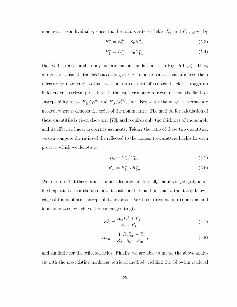
nonlinearities individually, since it is the total scattered fields, E+3 and E−1 , given by
E+3 = E+
3e + Z0H+3m, (5.3)
E−1 = E−1e − Z0H−1m, (5.4)
that will be measured in any experiment or simulation, as in Fig. 5.1 (a). Thus,
our goal is to isolate the fields according to the nonlinear source that produced them
(electric or magnetic) so that we can run each set of scattered fields through an
independent retrieval procedure. In the transfer matrix retrieval method the field-to-
susceptibility ratios E+3e/χ
(α)e and E−1e/χ
(α)e , and likewise for the magnetic terms, are
needed, where α denotes the order of the nonlinearity. The method for calculation of
these quantities is given elsewhere [70], and requires only the thickness of the sample
and its effective linear properties as inputs. Taking the ratio of these two quantities,
we can compute the ratios of the reflected to the transmitted scattered fields for each
process, which we denote as
Re = E−1e/E+3e, (5.5)
Rm = H−1m/H+3m. (5.6)
We reiterate that these ratios can be calculated analytically, employing slightly mod-
ified equations from the nonlinear transfer matrix method, and without any knowl-
edge of the nonlinear susceptibility involved. We thus arrive at four equations and
four unknowns, which can be rearranged to give
E+3e =
RmE+3 + E−1
Re +Rm
, (5.7)
H+3m =
1
Z0
ReE+3 − E−1
Re +Rm
, (5.8)
and similarly for the reflected fields. Finally, we are able to merge the above analy-
sis with the pre-existing nonlinear retrieval method, yielding the following retrieval
88

equations:
χ(α)e =
RmE+3 +E−1
Re+Rm
E+3e/χ
(α)e
, (5.9)
χ(α)m =
1Z0
ReE+3 −E
−1
Re+Rm
H+3m/χ
(α)m
. (5.10)
These represent slight modifications to the former nonlinear retrieval equations. In
contrast to the previous method, these equations make use of both the transmitted
and reflected spectrums, but still require measurements from only a single experiment
or simulation. However, Eqs. (5.9) and (5.10) now retrieve both electric and magnetic
contributions in a given nonlinear process, allowing for the complete characterization
of more general NLMMs. While the presence of both electric and magnetic nonlinear
susceptibilities is rare for naturally occurring materials, the situation is very common
for NLMMs, thus motivating the modifications considered here.
The modified retrieval procedure described above is sufficient to analyze the struc-
tures in the following sections. We note, however, that we ignore any effects due to
magnetoelectric coupling between unit cells either in the fundamental or the har-
monics. Because magnetoelectric coupling appears to be of concern only when both
the electric and magnetic responses are simultaneously resonant, its neglect here is
reasonable for the configurations we consider. [106, 107, 77, 78]
5.2 Simulations and retrievals
In this section, we analyze the nonlinearity enhancement effect in the context of four
distinct types of NLMM structures: the electric-field-coupled resonator (ELC), the
split-ring resonator (SRR), the cut-wire medium, and the I-beam medium. The non-
linearity in each case comes from a generic nonlinear dielectric matrix in which the
metallic structure is embedded. Full-wave, frequency domain simulations, using the
89
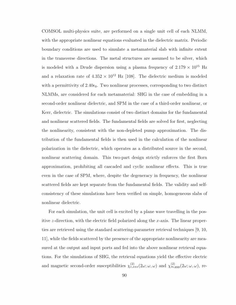
COMSOL multi-physics suite, are performed on a single unit cell of each NLMM,
with the appropriate nonlinear equations evaluated in the dielectric matrix. Periodic
boundary conditions are used to simulate a metamaterial slab with infinite extent
in the transverse directions. The metal structures are assumed to be silver, which
is modeled with a Drude dispersion using a plasma frequency of 2.179 × 10¹⁵ Hz
and a relaxation rate of 4.352 × 10¹² Hz [108]. The dielectric medium is modeled
with a permittivity of 2.40ε0. Two nonlinear processes, corresponding to two distinct
NLMMs, are considered for each metamaterial: SHG in the case of embedding in a
second-order nonlinear dielectric, and SPM in the case of a third-order nonlinear, or
Kerr, dielectric. The simulations consist of two distinct domains for the fundamental
and nonlinear scattered fields. The fundamental fields are solved for first, neglecting
the nonlinearity, consistent with the non-depleted pump approximation. The dis-
tribution of the fundamental fields is then used in the calculation of the nonlinear
polarization in the dielectric, which operates as a distributed source in the second,
nonlinear scattering domain. This two-part design strictly enforces the first Born
approximation, prohibiting all cascaded and cyclic nonlinear effects. This is true
even in the case of SPM, where, despite the degeneracy in frequency, the nonlinear
scattered fields are kept separate from the fundamental fields. The validity and self-
consistency of these simulations have been verified on simple, homogeneous slabs of
nonlinear dielectric.
For each simulation, the unit cell is excited by a plane wave travelling in the pos-
itive z-direction, with the electric field polarized along the x-axis. The linear proper-
ties are retrieved using the standard scattering-parameter retrieval techniques [9, 10,
11], while the fields scattered by the presence of the appropriate nonlinearity are mea-
sured at the output and input ports and fed into the above nonlinear retrieval equa-
tions. For the simulations of SHG, the retrieval equations yield the effective electric
and magnetic second-order susceptibilities χ(2)e,xxx(2ω;ω, ω) and χ
(2)m,yyy(2ω;ω, ω), re-
90

spectively. For SPM, the retrieved parameters are the effective electric and magnetic
third-order susceptibilities χ(3)e,xxxx(ω;ω,−ω, ω) and χ
(3)m,yyyy(ω;ω,−ω, ω), respectively.
Though the local fields will inevitably contain multiple field components, the bound-
ary conditions at the ports enforce the scattered waves to be the same polarization
as the incident wave. Thus, even though the local fields will probe all elements of
the local nonlinear tensor in the dielectric, the simulations will ultimately investi-
gate just a single element of each of the NLMM’s effective nonlinear tensors. The
polarization and orientation used in the following simulations were chosen to ensure
maximum coupling between the incident wave and the structure. Though it is not
presented here, the full effective linear and nonlinear tensors can be retrieved by
the same procedure, provided that the appropriate polarizations of the various con-
tributing waves are enforced. In the following subsections, the tensorial notation in
the material properties is omitted for brevity.
The higher-order susceptibility alone, however, is not an adequate measure of the
enhancement over the bulk embedding medium, due to the simultaneous effect of
the periodic inclusions on the medium’s impedance. Instead, we define the material
figure of merit (see Appendix),
κ(2) =Z(ω)
√Z(2ω)
Z0
χ(2)e +
Z0
Z(ω)√Z(2ω)
χ(2)m , (5.11)
where Z(ω) =√
µ(ω)ε(ω)
is the effective impedance of the NLMM and Z0 is the impedance
of free-space. This is a slight modification to the usual definition in a purely electric
medium [109] (p. 445). With this definition, the corresponding material figure of
merit of the nonlinear dielectric alone is
κ(2)d =
Z3/2d
Z0
χ(2)d , (5.12)
where the subscript d refers to the properties of the dielectric. For consistency, we
91

Figure 5.2: (Reproduced with permission from Ref. [84]. Copyright (2011) by theAmerican Physical Society.) (a) An ELC embedded in a nonlinear dielectric. (b) Theelectric field norm at the resonance frequency. (c) The retrieved linear properties.(d) Log-scale plot of the second- and third-order electric field localization factors (Eq.(5.15)). (e-j) The retrieved electric and magnetic higher-order susceptibilities andcorresponding material figures of merit, normalized by the nonlinear bulk dielectric:(e-g) are the second-order properties corresponding to SHG and (h-j) are the third-order properties corresponding to SPM. The real (solid blue curve) and imaginary(dashed green curve) parts are shown for the higher-order susceptibilities.
define an analogous material figure of merit for SPM,
κ(3) =Z(ω)2
Z0
χ(3)e +
Z0
Z(ω)2χ(3)m , (5.13)
with units of m2/W. It can be shown that the first-order correction in the power-
dependent refractive index is directly related to this figure and given by ∆n = 34κ(3)I,
where I is the field intensity. The material figure of merit in the third-order nonlinear
dielectric alone is given by
κ(3)d =
Z2d
Z0
χ(3)d . (5.14)
We reiterate here that the deviations of the NLMM’s effective nonlinearities from
92

that of the embedding medium are not due to the addition of nonlinearities, as we
neglect the nonlinearity of the metal structures themselves, but rather come from
the induced localization of the fundamental fields within the embedding dielectric.
Additionally, since the retrieved properties are necessarily a sort of average over the
whole unit cell, it may seem that the small volumes in which the majority of the
field localization occurs will have the effect of counterbalancing the enhancement.
Indeed, the additional nonlinear activity in the areas of high field concentration will
be accompanied by reduced nonlinear activity in the areas of low field concentration.
However, since the local nonlinear effects scale as higher-order powers of the local
fields, the field localization is in effect weighted more strongly than the effective
reduction in contributing volume, and, consequently, the bulk nonlinear susceptibility
must take on a larger value than the background medium alone. To measure the
degree of field localization, we introduce the localization factor, analogous to the
enhancement factors employed in previous plasmonic studies [97, 98],
L(|E|α) =
∫V|EMM(~r)|αd~r3∫
V|Ehom(~r)|αd~r3
, (5.15)
where the numerator is a volume integral of the fundamental electric field norm
raised to the α power, integrated over the metamaterial unit cell. The denominator
is the same integral but for a homogeneous slab with equivalent linear properties.
Thus, L(|E|α) is a direct measure of the degree of inhomogeneity in the fields within
the metamaterial, normalized by an otherwise equivalent homogeneous medium. As
we show in the following subsections, the deviations of the NLMM’s effective non-
linearities from that of the embedding medium can be quite dramatic, especially
when the structures are operated near resonance, where the second- and third-order
localization factors reach their maximums.
93

5.2.1 The nonlinear electric-field-coupled resonator (ELC)
The ELC is a resonant metamaterial structure designed to exhibit an electric res-
onance [110]. The dominant coupling of the incident fields into and out of this
structure is capacitive, and thus it is classified as an electric resonator. At reso-
nance, the incident electric fields become highly confined in the capacitive gaps, as
shown in Fig. 5.2 (b), making this an ideal structure for the resonant enhancement
of the nonlinearities of any medium placed in these gaps.
The ELC employed here, displayed in Fig. 5.2 (a), is composed of 50 nm thick,
100 nm wide silver with two 100 nm gaps. The outer dimensions of the silver pattern
are 1.6 µm, while the ELC itself is arranged in a cubic lattice with a lattice constant
of 2 µm. For the SHG simulation, the nonlinear dielectric is given a non-zero second-
order electric susceptibility for both fundamental and harmonic fields polarized in the
x-direction. All other elements of the nonlinear tensors, both second- and third-order,
are zero. For SPM, the dielectric’s nonlinearity takes the form of a non-zero third-
order electric susceptibility for fields polarized in the x-direction. The retrieved linear
properties are shown in Fig. 5.2 (c). The retrieved values of the second-order and
third-order susceptibilities and material figures of merit, normalized by the nonlinear
dielectric, are displayed in Fig. 5.2 (e-j). The higher-order magnetic susceptibilities
are normalized by the impedance of free-space where appropriate.
As expected, the retrieved nonlinearities of the ELC show massive enhancements
near the ELC’s resonance. The second-order and third-order figures of merit show
peak values that are two orders and four orders of magnitude larger than the em-
bedding nonlinear dielectric, respectively. The retrieved nonlinear susceptibilities
themselves also show the expected Lorentzian features in their real and imaginary
parts. It is noteworthy that the second-order properties show weaker (one order of
magnitude) enhancements when the fundamental frequency corresponds to half the
94
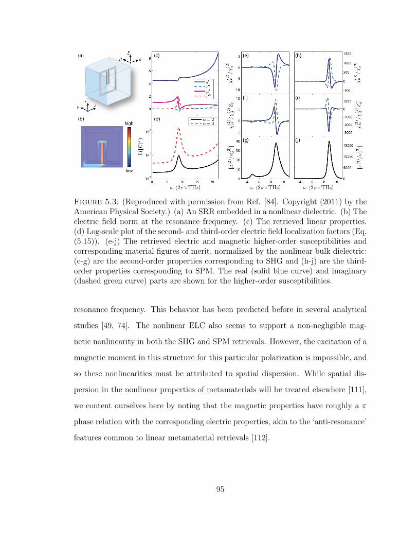
Figure 5.3: (Reproduced with permission from Ref. [84]. Copyright (2011) by theAmerican Physical Society.) (a) An SRR embedded in a nonlinear dielectric. (b) Theelectric field norm at the resonance frequency. (c) The retrieved linear properties.(d) Log-scale plot of the second- and third-order electric field localization factors (Eq.(5.15)). (e-j) The retrieved electric and magnetic higher-order susceptibilities andcorresponding material figures of merit, normalized by the nonlinear bulk dielectric:(e-g) are the second-order properties corresponding to SHG and (h-j) are the third-order properties corresponding to SPM. The real (solid blue curve) and imaginary(dashed green curve) parts are shown for the higher-order susceptibilities.
resonance frequency. This behavior has been predicted before in several analytical
studies [49, 74]. The nonlinear ELC also seems to support a non-negligible mag-
netic nonlinearity in both the SHG and SPM retrievals. However, the excitation of a
magnetic moment in this structure for this particular polarization is impossible, and
so these nonlinearities must be attributed to spatial dispersion. While spatial dis-
persion in the nonlinear properties of metamaterials will be treated elsewhere [111],
we content ourselves here by noting that the magnetic properties have roughly a π
phase relation with the corresponding electric properties, akin to the ‘anti-resonance’
features common to linear metamaterial retrievals [112].
95

5.2.2 The nonlinear split-ring resonator (SRR)
The second structure we consider is the SRR, displayed in Fig. 5.3 (a), which also
exhibits an LC-type resonance. In contrast to the ELC, however, the dominant
coupling in this structure is inductive, coming from magnetic flux passing through
the interior of the metallic ring. As such, the SRR is a magnetic resonator, and on
resonance the electric fields, shown in Fig. 5.3 (b), become highly confined in the
capacitive gap. Though the only nonlinearity present is the electric nonlinearity of
the dielectric medium, the coupling of the generated electric fields to the magnetic
resonance of the SRR makes the dominant effective nonlinearity magnetic in nature.
Like the ELC, the SRR is composed of 50 nm thick, 100nm wide silver, but with
a single 100 nm gap. The outer dimensions and lattice constant are identical to the
ELC. However, since the capacitive gap is rotated compared to the ELC, the highly
localized electric fields of the SRR are dominantly in the z-direction. Thus, the
dielectric’s nonlinearities considered in these simulations only involve fields polarized
in the z-direction and, again, all other elements of the dielectric’s nonlinear tensors
are set to zero. The retrieved linear, second-order, and third-order properties are
displayed in Fig. 5.3 (c-j).
Again, for excitation near the resonance frequency of the SRR, the retrieved non-
linearities are highly enhanced compared to the bulk nonlinear dielectric. Many of
the same features in the retrieval of the ELC are present, but with the difference
that the effective nonlinearities are mostly magnetic in nature. The spatial disper-
sion effects are also slightly mitigated due to the lower resonance frequency of the
SRR. Furthermore, while the SPM material figure of merit is slightly larger for the
SRR, the ELC shows roughly double the enhancement in SHG. This can be explained
in terms of the necessary overlap of the field distributions at the fundamental and
second-harmonic frequencies required for efficient conversion in a bulk material, sim-
96

Figure 5.4: (Reproduced with permission from Ref. [84]. Copyright (2011) bythe American Physical Society.) (a) A cut-wire medium embedded in a nonlineardielectric. (b) The electric field norm at 10 THz. (c) The retrieved linear properties.(d) Log-scale plot of the second- and third-order electric field localization factors (Eq.(5.15)). (e-j) The retrieved electric and magnetic higher-order susceptibilities andcorresponding material figures of merit, normalized by the nonlinear bulk dielectric:(e-g) are the second-order properties corresponding to SHG and (h-j) are the third-order properties corresponding to SPM. The real (solid blue curve) and imaginary(dashed green curve) parts are shown for the higher-order susceptibilities.
ilar to the nonlinear coupling between different modes in a waveguide. Because the
x-component of the local electric field is dominant at all frequencies in the ELC, the
coupling between the field distributions at different frequencies is more efficient than
in the SRR, where the z-component of the local electric field is only strong for fre-
quencies sufficiently close to the resonance. For SPM, where all involved frequencies
are degenerate, the mode overlap is identically unity in both structures.
5.2.3 The nonlinear cut-wire medium
The cut-wire medium, on the other hand, can be employed as a non-resonant meta-
material, often to provide a relatively broadband electric response. Though this
97

medium will lack the dramatic resonance-induced enhancements of the SRR and
ELC, it supports an inhomogeneous field distribution, as seen in Fig. 5.4 (b), with
electric fields weakly confined to the capacitive gap between neighboring cut-wires.
Like the ELC, coupling between this structure and the incident fields is capacitive
in nature.
The cut-wire structure, shown in Fig. 5.4 (a), is composed of a silver rectangular
rod, 100 nm thick, 200 nm wide, with a gap of 100 nm between neighboring cut-
wires. These dimensions are thicker than the previous structures in order to reduce
the cut-wire’s effective inductance, ensuring operation well below the structure’s
resonance. The lattice constant is 2 µm in all directions. For the SHG simulation,
the embedding dielectric is given a non-zero second-order electric susceptibility for
both fundamental and harmonic fields polarized in the x-direction. For SPM, the
dielectric’s nonlinearity takes the form of a non-zero third-order electric susceptibility
for fields polarized in the x-direction. The retrieved linear, second-order, and third-
order properties are displayed in Fig. 5.4 (c-j).
The retrieved nonlinearities of the cut-wire medium are very different from the
previous two resonant structures. For a fundamental frequency of 10 THz, roughly
the frequency of interest for this analysis, the enhancement in SHG is 5-fold, while
the nonlinearity for SPM is 56 times greater than the nonlinear dielectric alone.
While these enhancements are much less dramatic than the resonant SRR and ELC,
they deserve some discussion. Unlike its resonant counterparts, the cut-wire medium
shows fairly broadband enhancements of the material figures of merit, asymptoting
at low frequencies to values greater than unity. Moreover, these enhancements are
not accompanied by significant losses. In fact, the effective loss tangents at 10 and 20
THz in the cut-wire medium are just 1.1× 10⁻³ and 2.8× 10⁻³, respectively. Spatial
dispersion effects are also much less prominent. Thus, there exists a significant trade-
off between resonant and non-resonant metamaterial structures in terms of enhancing
98

Figure 5.5: (Reproduced with permission from Ref. [84]. Copyright (2011) bythe American Physical Society.) (a) An I-beam structure embedded in a nonlineardielectric. (b) The electric field norm at 10 THz. (c) The retrieved linear properties.(d) Log-scale plot of the second- and third-order electric field localization factors (Eq.(5.15)). (e-j) The retrieved electric and magnetic higher-order susceptibilities andcorresponding material figures of merit, normalized by the nonlinear bulk dielectric:(e-g) are the second-order properties corresponding to SHG and (h-j) are the third-order properties corresponding to SPM. The real (solid blue curve) and imaginary(dashed green curve) parts are shown for the higher-order susceptibilities.
nonlinear phenomena.
5.2.4 The nonlinear I-beam structure
The I-beam structure belongs to the same category of non-resonant electric meta-
materials as the previous cut-wire medium, but with the extended arms providing
additional capacitance. Due to the increased capacitance, the I-beam supports a
stronger electric response and confines a greater fraction of the incident field to the
gaps between neighboring structures than the cut-wire medium, as seen in Fig. 5.5
(b) and (d). Thus, this medium can be expected to show a strong, broadband en-
hancement of the embedding medium’s nonlinearities.
99

The I-beam, displayed in Fig. 5.5 (a), consists of 100 nm thick, 200 nm wide sil-
ver in the shape of an ‘I’, with arms that extend 1.6 µm from tip-to-tip. The lattice
constant and gap between neighboring I-beams are 2 µm and 100 nm, respectively.
The embedding dielectric used is the same as the nonlinear cut-wire and ELC medi-
ums. The retrieved linear, second-order, and third-order properties are displayed in
Fig. 5.5 (c-j).
As expected, the I-beam structure shows similar features to the cut-wire medium,
but with much larger overall enhancements. For a fundamental frequency of 10 THz,
the SHG and SPM material figures of merit are enhanced by a factor of 55 and 400,
respectively, both roughly an order of magnitude larger than the cut-wire medium.
However, the useable frequency range of the I-beam structure is significantly reduced:
the capacitance is so large that the resonance frequency of this structure is brought
into view. The massive spatial dispersion in both the linear and nonlinear properties
call into question the validity of the SHG retrieval at 10 THz, as the second-harmonic
frequency passes through the resonance frequency well below the 10 THz target
frequency for the fundamental. However, the low frequency asymptotic value for
SHG is still valid, as well as the SPM results, which do not suffer from involving a
frequency at twice the fundamental frequency. Additionally, at 10 THz, the effective
loss tangent is 1.1 × 10⁻², more than small enough to consider the nearly three
orders of magnitude enhancement in the SPM material figure of merit a low-loss,
non-resonant effect. Thus, there exists a trade-off between the cut-wire and I-beam
structures, where the operational frequencies, the loss tangent, and the magnitude
of the enhancement can be weighed against one another for a given application.
5.3 Calculation of the nonlinear conversion efficiencies
The retrieved parameters of the previous section fully characterize the four nonlinear
metamaterials, allowing for the metamaterials to be analyzed as if they were per-
100

fectly homogeneous materials. Thus, we are in a position to give a more thorough
analysis of the NLMMs in terms of their applicability in realistic nonlinear devices.
In particular, the NLMMs presented here offer competing effects in the enhance-
ment of nonlinear phenomena: on the one hand, they show nonlinearities that are
orders of magnitude larger than the embedding medium alone; on the other hand,
the periodic metallic inclusions are a major source of ohmic losses, constraining the
maximum lengths of any resulting devices. Before NLMMs can be endorsed as an
avenue to improving on existing nonlinear devices, the NLMM enhancement effect
must be weighed against the accompanying losses in the context of realistic device
specifications. In this section, using a coupled mode theory derived for homogeneous
materials, we calculate the figures of merit and conversion efficiencies for nonlinear
devices based on slabs of the four NLMMs, analyzing both the second- and third-
order processes. We show that, despite the severe constraints imposed by material
losses, the NLMMs are able to support reasonable conversion efficiencies in the form
of compact, even subwavelength, devices.
5.3.1 Second-harmonic generation
SHG from a monochromatic, planar wave, travelling in a homogeneous second-order
nonlinear medium, can be described by a coupled mode analysis. Using the simplify-
ing assumptions of non-depleted pump and slowly varying amplitude, the following
expression can be derived for the output second-harmonic intensity [109]:
Iout(2ω) =ω2
2c2|κ(2)|2[Iin(ω)]2L2h(L), (5.16)
where L is the total interaction length, Iin(ω) is the input intensity of the fundamental
wave, and
h(L) = exp
[−(α(2ω)
2+ α(ω)
)L
][sinh(∆αL/2)]2
(∆αL/2)2(5.17)
101

contains the contributions from the absorption coefficients (α(ω)) at both frequencies,
and ∆α is given by
∆α =α(2ω)
2− α(ω). (5.18)
Note that, for the sake of narrowing the focus of the analysis, the terms dependent
on the phase mismatch between the interacting waves have been removed.
From the above, we can define the system’s conversion efficiency as
η(2) =Iout(2ω)
Iin(ω)=ω2
2c2|κ(2)|2L2h(L)Iin(ω). (5.19)
In determining the maximum efficiency and the corresponding device length for SHG,
we find the quantity L2h(L) to be maximized by an optimum interaction length
Lopt =2
∆αtanh−1
(∆α
α(2ω)/2 + α(ω)
). (5.20)
For interaction lengths longer than Lopt, linear absorption begins to dominate, and
the conversion efficiency declines.
We use Eqs. (5.19) and (5.20), together with the retrieved parameters of the
four NLMMs, to calculate realistic device sizes and efficiencies. For the ELC and
SRR, we choose optimum fundamental frequencies close to the respective resonance
frequencies to maximize the resonant enhancement. A fundamental frequency of 10
THz is used for the cut-wire medium, while the I-beam structure, to avoid significant
spatial dispersion, is operated at 5 THz, noting that the efficiencies of these non-
resonant structures are characteristic of broad frequency bands. The ratio of the
efficiencies of the NLMMs to the nonlinear dielectric alone is given by
F (η(2)) =η(2)
η(2)d
= h(L)
∣∣∣∣∣κ(2)
κ(2)d
∣∣∣∣∣2
. (5.21)
102

This quantity directly compares devices of the same lengths, operating frequencies,
and input powers, while taking into account both the enhancement effect and the
additional losses introduced by the periodic metallic inclusions. Thus, F (η(2)) repre-
sents a complete, albeit simplistic, measure of the relative performances of NLMMs
and natural materials as frequency doublers. The optimum lengths and efficien-
cies for all four NLMMs are displayed in Table 5.1, assuming a value of χ(2)d = 20
pm/V for the embedding nonlinear dielectric, and an input intensity of Iin(ω) = 40
MW/cm2.
Table 5.1: (Reproduced with permission from Ref. [84]. Copyright (2011) by theAmerican Physical Society.) Optimal lengths, efficiencies, and normalized efficienciesfor SHG in each NLMM. The conversion efficiencies are calculated using the valueχ
(2)d = 20 pm/V for the nonlinear dielectric, and assuming an input intensity of 40
MW/cm2.
NLMM ω (2π×THz) Lopt (µm) η(2) (×10−6) F (η(2))ELC 11.4 4 8.65 1170SRR 8.6 4 1.07 253cut-wire 10 650 456.12 3.03I-beam 5 216 132.32 31.9
Though the above analysis ignores the role of phase matching, this interesting
and crucial factor deserves a few words. In principal, conventional approaches to
phase matching [49] should be largely applicable to NLMMs based on periodic in-
clusions in a nonlinear dielectric by applying the same techniques to the embedding
medium itself. However, due to the range and configurability in their linear proper-
ties, NLMMs may offer unique advantages in overcoming phase mismatch. For exam-
ple, a number of recent studies have revealed novel configurations for phase matching
and quasi-phase matching (QPM) that are singular to NLMMs [113, 114, 89, 115].
Furthermore, the relatively small interaction lengths proposed in Table 5.1 have the
added effect of relaxing the constraints imposed by phase mismatch. As a numerical
example, the coherence length in the nonlinear ELC for a fundamental frequency of
103

11.4 THz is Lcoh = 2π/∆k = 14.9 µm, which is actually larger than the optimum
interaction length, making phase mismatch essentially a non-factor in this structure.
Thus, phase matching should not pose a significant challenge to the implementation
of NLMMs in nonlinear devices, and could ultimately prove to be an advantage. A
detailed analysis of phase matching in NLMMs will be treated in the next chapter.
5.3.2 Self-phase modulation
Among third-order nonlinear processes, SPM has unique applications with its own
set of definitions and figures of merit. However, since it is our intention to investigate
the enhancement properties of NLMMs on third-order processes in general, we omit
a discussion of the particulars of SPM and instead describe the process through a
coupled mode analysis, analogous to SHG. Specifically, we continue to invoke the non-
depleted pump approximation, and calculate the intensity of the nonlinear scattered
fields. Though the non-depleted pump is inappropriate for describing most devices
involving SPM, such as directional couplers, the following analysis and figures of
merit have the advantage of being readily applicable to third-order processes in
general, such as non-degenerate four-wave mixing. For a more detailed analysis of
metamaterials for optical switching and related applications, the reader is referred
to Ref. [38].
Let us consider a monochromatic, planar wave, travelling in a homogeneous third-
order nonlinear medium. In the non-depleted pump limit and taking the slowly
varying amplitude approximation, we can describe the SPM process in terms of the
intensity of the nonlinear scattered fields, given by
INLout(ω) =
9
16
ω2
c2|κ(3)|2L2g(L)
[IFF
in (ω)]3, (5.22)
where
g(L) = exp [−2α(ω)L] (5.23)
104

contains the effect of propagation losses on efficiency. It follows that the conver-
sion efficiency is given by the ratio of the nonlinear scattered intensity to the input
intensity,
η(3) =INL
out(ω)
IFFin (ω)
=9
16
ω2
c2|κ(3)|2L2g(L)
[IFF
in (ω)]2
(5.24)
As before, we find an optimum interaction length by maximizing the quantity L2g(L),
so that maximum efficiency is obtained for a slab of length
Lopt =1
α(ω). (5.25)
Normalizing Eq. (5.24) by the efficiency of the dielectric alone, we arrive at the
figure of merit describing the enhancement of third-order nonlinear process in the
four NLMMs:
F (η(3)) =η(3)
η(3)d
= g(L)
∣∣∣∣∣κ(3)
κ(3)d
∣∣∣∣∣2
. (5.26)
The optimum lengths and conversion efficiencies for SPM in the four NLMMs are
displayed in Table 5.2, assuming a value of χ(3)d = 10−20 m2/V2 for the embedding
nonlinear dielectric, and an input intensity of Iin(ω) = 40 MW/cm2.
Table 5.2: (Reproduced with permission from Ref. [84]. Copyright (2011) by theAmerican Physical Society.) Optimal lengths and conversion efficiencies for SPM in
each NLMM. The conversion rates are calculated using the value χ(3)d = 10−20 m2/V2
for the nonlinear dielectric.
NLMM ω (2π×THz) Lopt (µm) η(3) (×10−7) F (η(3))ELC 11.5 2 4.25 8.25× 10⁶
SRR 8.7 2 8.70 2.95× 10⁷
cut-wire 10 1124 51.28 417I-beam 10 66 9.39 2.21× 10⁴
In the resonant structures for both the second-order and third-order nonlinear
processes, however, the linear absorption in the metamaterials is strong enough to
potentially invalidate the slowly varying amplitude approximation. In order to verify
105

the above results, the conversion efficiencies of the ELC and SRR were calculated
directly using the nonlinear transfer matrix method [68], finding the error to be less
than 25% in all cases.
5.4 Anisotropy and poling in the effective nonlinear tensors
Within an inhomogeneous medium, the local fields can vary quite dramatically from
the macroscopic and applied fields, both in magnitude and direction [59, 116, 117].
While field concentration has been a driving force in the search for metamaterials
and plasmonic media with enhanced nonlinear coefficients [2, 118, 102, 84, 54, 56],
control over field orientation has received less attention. However, it is this control
of the directionality of the local fields that allows access to effective properties of
fundamentally different natures than the constitutive materials. Not only can meta-
materials lead to effective magnetic and magneto-electric behavior, but they can also
control the anisotropy of optical properties. In effect, manipulating the directionality
of the local fields in metamaterials can supplement the overall enhanced coefficients,
while offering additional degrees of functionality and flexibility. The following section
is reproduced with permission from Alec Rose, Ryan Latterman, David R. Smith,
and Philip Sullivan, Applied Physics Letters 103, 031102, 2013. Copyright (2013) by
the American Institute of Physics.
If we assume a metamaterial with negligible magnetism and losses, we can employ
the coupled-mode theory of chapter 4 to relate the effective χ(2) to overlap integrals
in the limit that the lattice constant is much smaller than a wavelength, [82]
χ(2)ijk =
1
V0
∫∫∫V0
dV ¯χ(2)(~r) : ~ej(~r)~ek(~r) · ~ei(~r), (5.27)
where ~en(~r) is the electric field of the Bloch mode with macroscopic polarization and
frequency indexed by n, and the integral is performed over a single unit-cell with
106

Figure 5.6: (Reproduced with permission from Ref. [119]. Copyright (2013)by the American Institute of Physics.) Sketch of a Pockels cell composed from ananoparticle-ONLO composite, with variable dimensions indicated (a). The gap sizeis controlled by the extent of the ONLO around the nanorod, while we define theoverlap as the percentage of the nanorod that coincides transversely with its nearestneighbors. Illustration of polymer ordering before (b) and after (c) a poling field isapplied to the medium.
volume V0. If the Bloch modes were nothing more than simple plane waves, as in
a homogeneous medium, then it is clear that the effective susceptibility would be a
simple volume average of the local one, and only the (typically) weaker off-diagonal
tensor elements could couple waves with orthogonal polarizations. However, due to
the inhomogeneous nature of the metamaterial, the local electric fields can overlap
despite the orthogonality of the macroscopic fields, leading to great flexibility in the
effective nonlinear tensors. The consequences of Eq. (5.27) are most evident in elec-
trooptics, indicating that a simple poling voltage in an inhomogeneous metamaterial
can lead to strong coupling of originally orthogonal polarizations. When one of these
polarizations is associated with the metamaterial’s internal resonance, the overall
107

effect can be quite dramatic. Moreover, an applied poling field or voltage can like-
wise induce local fields that are much stronger, or even differently oriented, than the
applied field, leading to poling thresholds and configurations that are distinct from
a simple bulk medium.
Figure 5.7: (a) Illustration of the nanorod-polymer array, with the basic rectangu-lar unit-cell indicated by the dashed red box. Plot of the real (b and c) and imaginary(d and e) parts of the effective indices for both polarizations.
As a demonstrative example, consider the simple idealized nanoparticle array
shown in Fig. 5.7 (a), consisting of gold nanorods 65 nm in length and 8 nm
in diameter, and coated in an organic nonlinear optical dielectric (ONLO) (ε =
2.19). These nematic-like (alternating) gold nanorods are loosely based on those in
Refs. [120, 121], and are known to support a polarization sensitive plasmonic reso-
nance [122]. Using a transfer-matrix based nonlinear retrieval method, we show that
this class of metamaterial supports a set of non-zero Pockels coefficients at telecom-
munication wavelengths that are both distinct in orientation and enhanced in mag-
nitude compared to the ONLO alone. By changing the interstitial spacing (gap)
and overlap between nearest neighbors, along with the choice of poling orientation,
108

we demonstrate a continuum of nonlinear tensor configurations and strengths. Ulti-
mately, metamaterials with this degree of control over the effective nonlinear tensor
can lead to Pockels cells with reduced dimensions and poling thresholds.
In the linear regime, fields normally incident on the surface of such a structure can
be decomposed into two orthogonal polarizations, corresponding to the electric field
parallel (z) and transverse (x) to the rod axis. For light with wavelength λ = 1530
nm, as in typical telecommunications systems, we can describe the anisotropic inter-
action through effective complex indices of refraction, nj = n′j + in′′j , applying the
well-known set of retrieval equations [11] to the results of finite-element simulations
(COMSOL multiphysics). We simulate a single unit-cell, defined by the dashed red
box in Fig. 5.7 (a), using periodic boundary conditions along the transverse bound-
aries and assuming a lattice constant of 100 nm in the direction of propagation (y).
The resulting effective indices are displayed in Fig. 5.7 (b). As expected, for certain
combinations of gap and overlap, the z polarization excites the dominant plasmonic
resonance at λ = 1530 nm, as evidenced by the strong peak in absorption (n′′z). At
the same time, the x polarization exhibits near transparency (nx ≈ 1). However,
it is interesting to note that despite such large anisotropy, both polarizations will
tend to excite significant electric fields in the gaps between adjacent nanorods, dom-
inantly oriented transverse to the rod surfaces. This is illustrated in Fig. 5.8 for DC
fields: while the macroscopic fields drive charge buildup in the individual nanorods,
the overlap between nearest neighbor nanorods focuses the energy into these gaps,
regardless of polarization.
In addition, this analysis immediately reveals the potential for lowering the effec-
tive poling thresholds in such a structure. Confinement of energy in small gaps must
be accompanied by local field enhancement, and so macroscopic poling fields can be
reduced while still achieving the required field strengths to pole the ONLO located
within the gaps. As a rough measure of this factor in poling threshold reduction, we
109

Figure 5.8: Schematic of the local fields (a and b) and estimate of the local fieldenhancement in the gaps between nanorods (c and d) for the two transverse polingconfigurations.
plot the local electric field at the center-point between two nanorods, normalized by
the applied field, as a function of gap and overlap in Fig. 5.8 (b) for both transverse
poling configurations. Both configurations display poling threshold reductions, while
the local directionality of the second-order material is now a function of the applied
field and the local structure.
In calculating the effective nonlinear coefficients of the nanorod metamaterial, we
turn to the recently developed transfer-matrix based retrieval method [67, 70], which
has shown success in determining the susceptibilities related to second-harmonic
generation and self-phase modulation in similar structures [83, 84]. In particular, we
investigate the Pockels effect, in which a propagating field is modified by the presence
110

of a strong DC or slowly varying electric field. However, a similar method could be
applied to determine effective wave-mixing coefficients.
Again using finite-element simulations via COMSOL multiphysics, we first sim-
ulate the poling field by applying a voltage in either of the transverse poling config-
urations. To simplify and generalize our results, we assume the ONLO will orient
itself completely in the direction of the local poling field, and only consider the local
nonlinear susceptibility along this axis. Next, we use the product of propagating and
DC fields to excite the ONLO according to its local nonlinear tensor, collecting the
re-radiated fields at the entrance and exit planes of the simulation, as in Ref. [84].
The nonlinear retrieval method is applied to this result to give the effective nonlinear
susceptibility, and the process is repeated for all possible permutations of poling and
propagating polarizations. From the nonlinear susceptibilities, we can calculate the
Pockels coefficients according to rijk =ε20εiεjχ
(2)ijk. For comparison, we consider elec-
trooptic modulation of the refractive indices, proportional to the material figure of
merit, (ninj)3/2rijk [49]. The magnitudes of these figures of merit are normalized by
n3r33 of the ONLO alone and plotted in Fig. 5.9, according to the usual contracted
index notation, for all non-zero elements in the two transverse poling configurations.
As expected, the coefficients r33 and r31 are largest in magnitude, enhanced by
more than an order of magnitude for the geometries that support plasmonic res-
onances close to the operational wavelength, λ = 1530 nm. The coefficients r51
and r53, though weaker, are interesting from an additional perspective: r51 and r53
represent the ability of a DC field to induce coupling between the two originally
orthogonal polarizations. In this way, the transparency of the x polarized wave can
be switched off by forcing it to couple to the inherently lossy plasmonic resonance
of the nanorods. This differs drastically from a homogeneous medium, which would
need to employ an ONLO that itself had large off-diagonal tensor elements, limiting
111

Figure 5.9: Magnitude of the Pockels coefficient figures of merit for the goldnanorod-ONLO array, (ninj)
3/2rijk, normalized by the figure of merit for the ONLOitself, in dB. The plots are separated by row, corresponding to the two transversepoling configurations, shown schematically: poling field along z (top row) and polingfield along x (bottom row).
the choice of materials and overall efficiency.
5.5 Appendix: Second-harmonic generation in a doubly nonlinearmedium
We present here a derivation of the second-harmonic intensity in a medium with
second-order nonlinear dependencies on the incident fields in both the electric po-
larization and magnetization. This analysis assumes plane waves with a single po-
larization, no losses, and real material parameters, but can be extended to these
more complex regimes by standard perturbations [66]. A similar development can
be employed for other three- and four-wave mixing processes in a doubly nonlinear
medium.
Let us consider a linearly polarized plane wave travelling with angular frequency
112

ω through a homogeneous, isotropic medium. We orient our axes such that the
electric field is along the x-axis, magnetic field along the y-axis, and propagation is
in the positive z-direction. Using the convention that ~E(z, t) =∑
n12~E(ωn)e−iωt, and
likewise for the other field variables, the x-component of the second-order electric
polarization at frequency 2ω is given by [49]
P (2)(2ω) =1
2ε0χ
(2)e (2ω;ω, ω) [E(ω)]2 , (5.28)
where, owing to the linear polarization of the involved fields, we have substituted
scalars for the usual vectors and tensors. The magnetization is defined in an analo-
gous way:
M (2)(2ω) =1
2χ(2)m (2ω;ω, ω) [H(ω)]2 , (5.29)
Thus, the material equations can be written as
D(2ω) = ε(2ω)E(2ω) + P (2)(2ω), (5.30)
B(2ω) = µ(2ω)H(2ω) + µ0M(2)(2ω), (5.31)
(5.32)
where ε(ω) and µ(ω) are the absolute, frequency-dependent permittivity and perme-
ability. For brevity, the frequency dependence of the field quantities will be denoted
through subscripts.
We start from Maxwell’s equations for time-harmonic fields, considering a second-
order polarization and magnetization,
∇× ~H2 = −i2ω(ε2 ~E2 + ~P (2)
), (5.33)
∇× ~E2 = i2ω(µ2~H2 + µ0
~M (2)), (5.34)
∇ · ~D2 = 0, (5.35)
∇ · ~B2 = 0. (5.36)
113

In the absence of the nonlinear terms, and with the above assumptions, Eqs. (5.33)
- (5.36) have solutions of the form
~E2 =(e+
2 exp(ik2z) + e−2 exp(−ik2z))x, (5.37)
~H2 =(h+
2 exp(ik2z) + h−2 exp(−ik2z))y, (5.38)
where k2 = 2ω√ε2µ2. We take the ansatz that the solutions in the presence of the
nonlinearities are simply a perturbation of the solutions to the linear problem, where
e±2 and h±2 are taken to be spatially varying in z. Furthermore, we assume the slowly
varying amplitude approximation, such that the forward and backward propagating
terms can be considered decoupled from each other and thus solved independently.
Focusing solely on the forward propagating terms, we substitute our trial solutions
into Eqs. (5.33) and (5.34), giving
−ik2H2 −dh2
dzexp(ik2z) = −i2ω
(ε2E2 + P (2)
), (5.39)
ik2E2 +de2
dzexp(ik2z) = i2ω
(µ2H2 + µ0M
(2)), (5.40)
We solve Eq. (5.39) for H2 and substitute this into Eq. (5.40),
ik2E2 +de2
dzexp(ik2z) =
i2ω
(Z2
(ε2E2 + P (2) +
i
2ω
dh2
dzexp(ik2z)
)+ µ0M
(2)
), (5.41)
where Z2 =√
µ2ε2
is the impedance of the medium. Rearranging and cancelling terms,
we arrive at the following expression:(de2
dz+ Z2
dh2
dz
)exp(ik2z) = i2ω
(Z2P
(2) + µ0M(2)), (5.42)
Next, we introduce the quantity γ = e2 + Z2h2 and use Eqs. (5.28) and (5.29) to
give
dγ
dz= iω
(Z2ε0χ
(2)e e2
1 + µ0χ(2)m h2
1
)exp(i∆kz), (5.43)
114

where ∆k = 2k1 − k2 is the phase mismatch.
For simplicity, we assume the non-depleted pump approximation, such that e1 and
h1 are constants that satisfy the linear form of Maxwell’s equations with e1 = Z1h1.
Thus, the above equation can be integrated over an interaction length L with the
boundary condition γ(0) = 0, giving
γ(L) = iω√Z2
e21
Z1
exp(i∆kL)− 1
i∆k(ε0Z1
√Z2χ
(2)e + µ0
1
Z1
√Z2
χ(2)m
). (5.44)
If at the point z = L a significant amount of second-harmonic field has built up, we
can take the approximation that |de2dz
(L)| and |µ0ωχ(2)m h2
1| are small compared to the
other terms in Eq. (5.40), implying that ik2E2(L) = i2ωµ2H2(L), or equivalently
e2(L) = Z2h2(L). Thus, in this limit, γ(L) = 2e2(L), and we find that
e2(L) = iω
2c
√Z2
Z1
e21κ
(2) exp(i∆kL)− 1
i∆k, (5.45)
where we have introduced the material figure of merit
κ(2) =Z1
√Z2
Z0
χ(2)e +
Z0
Z1
√Z2
χ(2)m , (5.46)
and Z0 is the impedance of free space. Looking at this equation, it is clear that
the electric field at the second-harmonic is a phase-sensitive superposition of the
contributions from the electric and magnetic nonlinearities alone. Subsequently, we
define the fundamental and second-harmonic intensities according to
I1 =1
2Z1
|e1|2 and I2(L) =1
2Z2
|e2(L)|2, (5.47)
and finally obtain
I2(L) =1
2
ω2
c2
∣∣κ(2)∣∣2 I2
1L2 sin2
(∆kL
2
)(∆kL
2
)2 . (5.48)
115

6
Metamaterial phase matching
In the presence of dispersion, the phase matching conditions are not automatically
satisfied and a wavevector mismatch will exist. The effect of this mismatch can be
visualized more clearly by considering the nonlinear material as an infinite collection
of radiation sources. The distribution and phase of each source is determined by
the polarization of the material, which in turn is dependent on both the material’s
properties and the incident radiation. As with an antennae array, the direction
and magnitude of the produced radiation is determined by the strength and relative
phases of the many sources. Dispersion tends to induce phase misalignment in these
radiation sources, and thus is often a prominent factor limiting the efficiency of
natural nonlinear materials. The advantage of metamaterials then, in this context, is
that they vastly extend the achievable range of linear and nonlinear properties. These
novel and often extreme properties, such as negative refraction, can offer a variety
of solutions to phase matching in wave-mixing processes. The following chapter
is reprinted with permission from Alec Rose, David R. Smith, Optical Materials
Express, 1, 1232, 2011. Copyright (2011) by The Optical Society.
We begin the analysis with the general expressions for phase matching, discussing
116

the conventional techniques and their usages and limitations. Next, we define five
broad categories of phase matching techniques in metamaterials: anomalous disper-
sion phase matching, birefringence phase matching, quasi-phase matching, negative-
index phase matching, and index-near-zero phase matching, which make up Sections
3 through 7. While Sections 3 through 5 discuss the application of conventional
techniques to metamaterials, Sections 6 and 7 outline unique phase matching con-
figurations that have only been achieved in metamaterials. In each case, numerical
and/or experimental examples are given to demonstrate the various forms of phase
matching. Finally, we conclude our paper in Section 8, summarizing our results and
offering an outlook for the potential applications of nonlinear metamaterials.
6.1 Wave-mixing and phase mismatch: an overview
Wave-mixing refers broadly to processes involving the interaction between multiple
photons, mediated by a nonlinear medium. As such, these processes are subject to
two major constraints: conservation of photon energy and conservation of photon
momentum. For simplicity, we will focus on three-wave mixing in a medium with a
bulk second-order nonlinear susceptibility, noting that the conclusions of this paper
can be extended to higher-order wave-mixing processes. For three-wave mixing of
plane waves in a homogeneous medium, energy and momentum conservation can be
written as
ω1 + ω2 = ω3 (6.1)
and
~k1 + ~k2 = ~k3, (6.2)
following the convention ω1 ≤ ω2 ≤ ω3. These equations apply to all three-wave
mixing processes, such as difference frequency generation, sum frequency generation,
and optical parametric amplification and oscillation. For the wave-mixing process
117

to be efficient, both Eqs. (6.1) and (6.2) must be satisfied to within the uncertain-
ties given by the system’s finite spatial and temporal extents [123]. Moreover, it is
convenient to define the phase mismatch ∆k =∣∣∣~k1 + ~k2 − ~k3
∣∣∣. The physical mean-
ing of the phase mismatch can be understood by considering the coherence length
Lcoh = 2π∆k
, which is the propagation length required for the lower-frequency and
high-frequency waves to complete a full phase cycle relative to each other. When the
phase matching condition is met, the coherence length becomes infinite.
Since the wave-mixing interaction requires spatio-temporal overlap between the
interacting waves, most systems are restricted to the case where the wavevectors are
co-linear. Taking propagation to be along the z-axis, we can write ~ki = ±niωicz,
where the ± corresponds to propagation in the positive/negative z-direction. We
summarize the four possible co-linear phase matching configurations in Table 6.1.
In labeling these configurations, we borrow the conventional notation of birefrin-
gent phase matching, such that Type I refers to like-propagating lower-frequency
waves, and Type II refers to unlike-propagating lower-frequency waves. While most
nonlinear devices to date are based on the parallel-I configuration, the anti-parallel
configurations are crucial to several highly intriguing and advantageous devices, such
as the mirror-less optical parametric oscillator (MOPO) [124, 125, 126, 127] and the
nonlinear optical mirror [113]. However, since all natural materials are constrained by
n > 0, the anti-parallel configurations require rather extreme techniques to overcome
phase mismatch [66].
Among artificial materials, metamaterials retain the advantage of being described
by homogenized, constitutive parameters. Moreover, the characterization and lan-
guage of nonlinear metamaterials has recently been extended to the standard for-
malism of nonlinear optics [74]. As such, the general equations and physics of wave
mixing processes and phase matching used in the analysis of natural nonlinear mate-
118

Table 6.1: (Reproduced with permission from Ref. [83]. Copyright (2011) by TheOptical Society.) Directions of Propagation and Corresponding Phase MatchingCondition for the Four Co-linear Three-Wave Mixing Configurations
Configuration ω1 ω2 ω3 Phase matching conditionparallel-I + + + n1ω1 + n2ω2 = n3ω3
anti-parallel-I + + - n1ω1 + n2ω2 = −n3ω3
anti-parallel-IIa - + + −n1ω1 + n2ω2 = n3ω3
anti-parallel-IIb + - + n1ω1 − n2ω2 = n3ω3
rials are equally applicable to metamaterials. The advantage of metamaterials then,
in this context, is that they vastly extend the achievable range of linear and nonlinear
properties. These novel and often extreme properties, such as negative refraction,
can offer a variety of solutions to phase matching in wave-mixing processes.
6.2 Anomalous dispersion phase matching
The parallel-I configuration is the simplest and most common wave-mixing setup,
in which all three waves propagate in the same direction. It is easily shown that,
considering waves of the same polarization and frequencies far from any absorption
features, the refractive index of a medium increases monotonically with frequency and
thus satisfaction of the phase matching condition given in Table 6.1 is impossible [49].
However, by carefully choosing these frequencies to be around a medium’s absorption
feature, the anomalous dispersion in this frequency range can, in principle, exactly
counteract the normal dispersion. This technique is known as anomalous dispersion
phase matching, and has been achieved, for example, in polymer waveguides through
the incoroporation of nonlinear chromophores with an absorption maximum between
the lower-frequency and high-frequency waves [128].
Many metamaterials are purposefully designed around an analogous absorption
feature, originating from a resonance in its constituent elements. As an example,
consider the split-ring resonator (SRR) medium, composed of a periodic array of
119

planar metallic rings with a capacitive gap [2]. The SRR displays an LC circuit
resonance, and has been shown to be characterized, in a range of frequencies around
its resonance, by a permeability [74]
µ(ω) = µ0
(1 +
Fω2
ω20 − ω2 − iγω
)(6.3)
where F is the oscillator strength, ω0 is the resonance frequency, and γ is the damping
coefficient. If we assume the nearly degnerate case ω1 ≈ ω2 and take the limit as
γ → 0, the phase matching condition can be simplified to
√√√√√1 +Fω2
1
ω20−ω2
1
1 +Fω2
3
ω20−ω2
3
=
√ε3ε1. (6.4)
where we have taken ni =√εiµi/ε0µ0, and εi is the permittivity seen by the ith
wave. Assuming the metamaterial contains no electrically resonant elements at these
frequencies and neglecting the effects of spatial dispersion, it follows that the per-
mittivity must display normal dispersion and thus the right hand side will be greater
than 1. To meet the phase matching condition, the frequencies must therefore satisfy
ω1 < ω0 < ω3. Furthermore, if, to avoid losses, the frequencies are equally detuned
from resonance such that ω20 −ω2
1 = ω23 −ω2
0 = 13ω2
0, then phase matching is achieved
with an oscillator strength of
F =δε
10 + 8δε, (6.5)
where δε = ε3−ε1ε1
. For δε ∼ 0.1, phase matching would require F ∼ 0.01. While
anomalous dispersion phase matching applies naturally to resonant metamaterials,
residual absorption in the transparency windows will tend to limit its applicability.
120

6.3 Birefringence phase matching
Alternatively, one can consider mixing between waves of differing polarizations, me-
diated by the appropriate off-diagonal elements of the nonlinear susceptibility tensor.
Thus, in an anisotropic medium, where the refractive index is dependent on a wave’s
direction of propagation and polarization, the phase matching conditions in Table
6.1 can potentially be satisfied by selecting the polarizations of the interacting waves.
The principal configurations for this technique, known as birefringent phase match-
ing, are generally divided into Types I and II, where Type-I involves lower-frequency
waves of the same polarization, and Type-II involves lower-frequency waves with
orthogonal polarizations. In a uniaxial crystal, propagation of ordinary and extraor-
dinary polarized waves is governed by the ordinary index noi and the extraordinary
index nei (θ) in the material, where
1
(nei (θ))2
=sin(θ)2
(nei )2
+cos(θ)2
(noi )2, (6.6)
nei is the principal value of the extraordinary index, and θ is the angle between
the optical axis and the direction of propagation. Thus, provided the birefringence is
large enough, the phase matching condition can be met by selecting the polarizations
of each wave and tuning θ through rotation of the crystal. As an example, let
us consider Type I-(eeo) phase matching in the nearly degenerate case, ω1 ≈ ω2.
For this configuration, phase matching can be achieved in a nonlinear crystal if the
maximum birefringence, ne3−no3, is greater than the material dispersion, ne3−ne1. This
condition is true of many anisotropic nonlinear crystals in the visible and infrared
spectral regions. However, for θ 6= 0, 180,±90, walk-off between the ordinary and
extraordinary beams imposes a limit on the maximum interaction length [48].
The anti-parallel configurations, on the other hand, require more extreme material
properties. For example, let us consider Type II-(eoo) birefringent phase matching
121

in the anti-parallel-IIa configuration for the nearly degenerate case, ω1 ≈ ω2, where
wave 1 is anti-parallel to waves 2 and 3. Invoking (eoo) polarizations in the refractive
indices of Table 6.1, phase matching in this case requires a birefringence of ne1−no1 ≥
2no3. Taking no3 ≈ no1, this constraint implies an extraordinary index that is roughly
three times the ordinary index, something no natural material has been found to
support. If instead ω1 << ω2, this constraint is relaxed, leading to speculation
that birefringent phase matching for backward wave oscillation will likely only be
achievable with a signal frequency in the mid- or far-infrared spectrum, while the
idler and pump are near-infrared or higher frequency waves [124].
In addition, birefringent phase matching requires a sufficiently strong cross-term
in the nonlinear tensor, corresponding to the direction of propagation and polar-
izations required by phase matching considerations. The strength of the various
cross-term nonlinear coefficients vary by material and are often identically zero due
to crystal symmetries [48]. These constraints on both the linear and nonlinear ten-
sors limit the desirable wave-mixing configurations, as well as the useable nonlinear
materials.
Metamaterials, meanwhile, have greatly extended the achievable types and mag-
nitudes of material anisotropy, introducing, for example, indefinite media [129].
Anisotropic metamaterials with extraordinary indices of refraction in excess of five
times the ordinary indices of refraction have been demonstrated at terahertz frequen-
cies [130]. Such large and configurable anisotropies can lift many of the conventional
limitations in applying birefringence phase matching to natural materials. In ad-
dition, engineering of the nonlinear tensor in metamaterials can ensure that the
particular cross-term involved is both non-zero and sufficiently large.
As a simple and demonstrative example, we consider a metamaterial composed
of overlapping silver bars arranged in a cubic lattice with a lattice constant of 1 µm,
immersed in a hypothetical nonlinear dielectric with εd = 2ε0 and d11 = 10 pm/V.
122

Figure 6.1: (Reproduced with permission from Ref. [83]. Copyright (2011) byThe Optical Society.) A nonlinear metamaterial consisting of overlapping silver barsembedded in a nonlinear dielectric, designed to operate as a birefringence phasematched MOPO. (a) Schematic of a single layer of the metamaterial, showing thepropagation direction and angle relative to the crystal axes. (b) The basic unit-cell ofthe metamaterial. (c) The retrieved extraordinary and ordinary indices of refraction.(d) Plot of the phase matched signal and idler frequencies as a function of angle. (e)Real and imaginary parts of the retrieved nonlinear coefficient.
Such a structure is easily fabricated by existing techniques, with a frequency range of
operation that includes the far-infrared wavelength of 10.6 µm, corresponding to the
output of a CO2 laser. Labeling the crystal axes as in Fig. 6.1(b), this metamate-
rial supports coupling between the structure and the incident fields only for electric
fields polarized in the Z-direction. Furthermore, the fields coupled into the structure
naturally localize in the capactive gaps between overlapping bars, with a dominant
electric field component in the X-direction. The symmetry of the metamaterial
prevents linear coupling between these polarizations, and thus the metamaterial is
strongly biaxial with effective linear susceptibility tensors that are diagonal in the
XY Z basis. The resulting nonlinear tensors, however, are not diagonal. Consider-
123

ing Type-I(eeo) and propagation in the Y Z-plane, there is significant overlap of the
X-components of the electric fields of the three modes in the capacitive gaps, and
the metamaterial thus supports a non-zero d35 nonlinear coefficient. This artificially
engineered nonlinearity, combined with the massive anisotropy, can support birefrin-
gence phase matched oscillations without a mirror, with distinct benefits compared
to alternate implementations.
To verify the linear and nonlinear properties, we implement full-wave, finite ele-
ment simulations on a single unit-cell of the nonlinear metamaterial using COMSOL
Multiphysics. We employ periodic conditions in the transverse directions and im-
plement a Drude model for the dielectric function of silver [108], using a plasma
frequency of 2179 THz and a collision frequency of 4.35 THz. We then retrieve
the linear properties via standard effective parameter retrieval techniques [11]. Con-
straining propagation to the Y Z plane, the metamaterial is positive uniaxial to within
simulation error, with extraordinary and ordinary waves corresponding to TM and
TE polarizations, respectively. The principal values of the extraordinary and ordi-
nary indices are shown in Fig. 6.1(c), displaying anomalously large birefringence, as
expected. Furthermore, we perform Type-I(eeo) difference frequency generation sim-
ulations using the techniques outlined in Ref. [84], using an ordinary-polarized 10.6
µm pump wave as wave 3, and sweeping the frequencies of waves 1 and 2. We use the
results of these simulations in the transfer matrix-based nonlinear retrieval method
to determine the d35 nonlinear coefficient [70], plotted in Fig. 6.1(e). Although the
cross-terms of the local nonlinear tensor in the dielectric are zero everywhere, the
metamaterial supports an effective d35 coefficient that is both non-zero and several
times larger than the d11 in the background dielectric, owing to the field localization
enhancement effect [84]. Renaming waves 1, 2 and 3 to signal, idler, and pump,
these results are immediately applicable to the nonlinear process of optical paramet-
ric oscillation. Indeed, the anisotropy is large enough to support birefringent phase
124

matching of a counter-propagating signal wave, corresponding to the anti-parallel-IIa
configuration. By rotating the direction of propagation z relative to the optical axis
Z, depicted in Fig. 6.1(a), the anti-parallel-IIa phase matching condition can be
satisfied for signal and idler frequency pairs over a wide frequency range, as shown in
Fig. 6.1(d). Thus, for pumping with a CO2 laser, this metamaterial can be expected
to support mirror-less oscillations, generating a tunable signal wave with a frequency
ranging from 1 to 8 THz. Moreover, the natural material chosen as the embedding
dielectric does not require significant birefringence nor nonlinear cross-terms, allow-
ing for high flexibility in the choice of embedding material, and, consequently, the
potential achievement of competitively-low oscillation thresholds. We note that the
large anisotropy, however, is accompanied by proportionately large walk-off, except
near θ = 90, corresponding to ω1 ≈ 2π × 8.18 THz and ω2 ≈ 2π × 20.10 THz.
Similarly, walk-off can be eliminated at any single signal-idler frequency pair by re-
designing the anisotropy of this metamaterial to ensure that the principal values of
the refractive indices satisfy the phase matching condition.
6.4 Quasi-phase matching
If instead we allow for an inhomogeneous medium, a third phase matching technique
becomes available. This technique, known as quasi-phase matching (QPM), relies on
the introduction of some sort of periodicity in the direction of propagation [131, 132].
Thus, the wavevectors can be conserved up to a multiple of the reciprocal lattice
vector ~G = 2πΛz, where Λ is the length of one period. Typically, the inhomogeneity
employed is a periodic modulation of the sign of the nonlinear susceptibility, called
periodic poling, but it can be much more general [133]. Including the contribution
from the periodicity in the above phase relations, QPM is achieved for ∆k = m~G, or
equivalently Λ = mLcoh, where m is any integer. As such, the possible frequencies
125

for phase matching are strictly limited by the choice of poling period, with small
associated tuning bandwidths [133]. The effective nonlinear coefficient of the wave-
mixing process, however, is necessarily reduced compared to the bulk value, with a
reduction factor of 2/π in the case of first-order QPM [49].
QPM in natural nonlinear crystals has been achieved for second-harmonic gener-
ation in the anti-parallel-I configuration [134] and for MOPO in the anti-parallel-IIa
configuration [135]. Due to the massive phase mismatch introduced by the backward-
propagating signal, the poling period required in the MOPO was a remarkable 800
nm. In principle, the other anti-parallel configurations presented in Table 6.1 can be
achieved in a similar fashion, though the fabrication constraints of such small pol-
ing periods will invariably limit the useable materials, frequencies, and interaction
lengths.
QPM extends naturally to metamaterials, which have proven viable options in
various laminar and gradient-style devices [136, 6]. At microwave frequencies, period-
ically poled QPM has been demonstrated by the precise orientation of the nonlinear
inclusion itself (see Fig. 6.2(a)) [89]. At infrared and visible frequencies, however,
the application of periodically poled QPM will depend on the metamaterial design.
In nonlinear metamaterials composed of periodic metallic structures embedded in
a nonlinear dielectric [84], for example, the conventional techniques of ferroelectric
domain engineering can be applied directly to the embedding dielectric. Assuming
it represents the dominant source of nonlinear activity, the reversal of the phase of
the embedding dielectric’s nonlinear susceptibility will necessarily cause an inversion
of the sign of the effective bulk nonlinearity. In any case, precise control of the
metamaterial unit-cell can allow for complex spatial distributions of the nonlinear
parameters for the purpose of QPM.
The generalized form of QPM, which utilizes a periodic variation in any of the
electromagnetic material properties, is particularly attractive in the special class of
126

Figure 6.2: (Reproduced with permission from Ref. [83]. Copyright (2011) byThe Optical Society.) (a) Diagram of the periodic poling technique employed inRef. [89] for the varactor-loaded split-ring resonator medium, whereby the phaseof the nonlinear coefficient is periodically flipped by reversing the orientation of thenonlinear element in each individual unit-cell. (b) Schematic of tunable parallel-I QPM difference frequency generation in an active metamaterial Bragg cell. Anexternal stimulus is used to produce a periodic variation in the linear properties ofthe metamaterial with a tunable period Λ.
active metamaterials. This stems from the fact that active metamaterials have been
shown to support dynamically tunable linear properties, using active mechanisms
such as photoconductivity, electrical bias, and temperature tuning [137, 138, 139, 30].
In such a system, one can envision introducing a periodic grating with a tunable
periodicity, analogous to an acoustically-induced Bragg cell but with a modulation
depth several orders of magnitude larger, depicted in Fig. 6.2(b) (see Appendix).
Thus, it was demonstrated theoretically that a wave-mixing process taking place in
an active metamaterial Bragg cell can support QPM over a widely tunable frequency
range [115]. However, active metamaterials of this kind can be difficult to realize for
frequencies above the THz regime. Furthermore, this form of tunable QPM comes
at the price of a largely reduced effective nonlinear coefficient.
127

6.5 Negative-index phase matching
One of the first and most exciting applications of metamaterials was the achieve-
ment of a negative index of refraction through the engineering of a composite with
both Re[ε] < 0 and Re[µ] < 0 in a certain frequency band [1, 4]. This, in turn,
spurred several theoretical studies of the nonlinear phenomena supported by nonlin-
ear negative-index mediums [140, 113, 114]. These studies showed that the phase
matching conditions of the anti-parallel wave-mixing configurations could be satis-
fied if the backward-propagating wave was in a negative-index band. This arises
from the fact that the wavevector and Poynting vector are oppositely directed in
a negative-index medium, such that a wave propagating in the negative z-direction
supports a positvely-directed wavevector. In particular, there were two processes that
proved highly intriguing from a theoretical viewpoint: mirror-less optical parametric
amplification and oscillation, and the nonlinear optical mirror effect.
The so-called nonlinear optical mirror effect is the name given to a device that
both converts the frequency of an incoming wave and redirects it backwards. As
originally conceived, the device operates via the degenerate case of the anti-parallel-I
configuration, in which the system is excited by a forward-propagating fundamen-
tal wave, generating a backward-propagating, or ‘reflected’, second-harmonic [113].
Thus, in a homogeneous medium, the phase matching condition is given by n1 = −n3
and requires either the fundamental or second-harmonic wave to propagate in a
negative-index band and the other in a positive-index band. Such a device has been
demonstrated at microwave frequencies, shown schematically in Fig. 7.5(b) [89]. The
dispersion relation of the nonlinear metamaterial was found to be
k(ω) = ω
õ
(εb
(1− ω2
c
ω2
)), (6.7)
128

where
µ = µ0
(1 +
Fω2
ω20 − iγω − ω2
). (6.8)
The various parameters were experimentally characterized, yielding F = 0.22, ω0 =
2π × 608 MHz, γ = 2π × 14 MHz, εb = 2.2ε0, and ωc = 2π × 674 MHz. The
corresponding index of refraction and coherence lengths are plotted in Fig. 7.5(a),
showing a dramatic rise in the coherence length of the anti-parallel-I configuration
as the fundamental wave is tuned through the negative-index band. Thus, owing
to negative-index phase matching, second-harmonic generation in the anti-parallel-I
configuration was shown to be far more efficient than in the parallel-I configura-
tion [89].
The mirror-less parametric processes could be achieved through either of the anti-
parallel-II configurations, employing wave 3 as a pump. The backward-propagating
wave provides an automatic feedback mechanism, removing the need for a mirror
and the associated calibrations and complexities. While the dynamics of a negative-
index MOPO are analogous to the previously discussed quasi-phase matched MOPO,
the materials involved and the nature of the phase matching are entirely different.
However, the losses associated with negative-index mediums will likely limit the
overall efficiencies of wave-mixing processes. Negative-index phase matching should
thus have its most meaningful applications in those devices specifically based on
negative refraction [141, 142].
6.6 Index-near-zero phase matching
Furthermore, there exists an interesting class of both natural materials and meta-
materials whose real parts of the refractive index vanish at some frequency, with
a number of intriguing characteristics as a consequence [143, 144]. In general, this
material property can be found near the plasma frequencies of various metals, or in
129

Figure 6.3: (Reproduced with permission from Ref. [83]. Copyright (2011) by TheOptical Society.) (a) Plot of the calculated coherence lengths for parallel-I (dashedpurple) and anti-parallel-I (solid orange) second-harmonic generation in a negative-index waveguide. The index of refraction at the fundamental frequency is included(dotted black), showing the negative-index and index-near-zero regimes (verticaldashed lines). (b) Schematic of the nonlinear optical mirror effect in negative-indexmetamaterial. (c) Schematic of simultaneous QPM in a periodically poled index-near-zero metamaterial. Si refers to the direction of energy flow of the ith wave.
any material with a sufficiently strong Lorentzian contribution to its material prop-
erties [? ]. If any of the waves involved in a wave-mixing process should propagate in
such an index-near-zero band, it can be seen from Table 6.1 that the phase match-
ing conditions of multiple unique configurations become degenerate. For example, if
n3 = 0, the anti-parallel-IIa and anti-parallel-IIb configurations are both satisfied by
n1ω1 = n2ω2. This characteristic of index-near-zero materials can be used to achieve
simultaneous phase or QPM of two or more configurations, opening avenues to a
wide range of simultaneous and/or cascaded nonlinear processes.
Indeed, simultaneous QPM of degenerate (ω1 = ω2) parallel-I and anti-parallel-I
configurations has been achieved at microwave frequencies, using the same metama-
terial described above by Eqs. (6.7) and (7.9), but in the region where n1 ≈ 0 [89].
Figure 7.5(a) demonstrates that, at the index-near-zero frequency given by the sec-
130

ond dashed vertical line, the coherence lengths of the parallel-I and anti-parallel-I
processes are equal. Thus, periodic poling was employed with a poling period of
Λ ≈ 2π∆k
, where ∆k ≈ |k3| for both configurations, so that an incident fundamental
wave was able to simultaneously generate second-harmonic waves in the positive and
negative z-directions, shown schematically in Fig. 7.5(c).
6.7 Conclusion
We have studied the potential phase matching solutions for nonlinear metamaterials
in the context of co-linear three-wave-mixing. We find that metamaterials support
multiple paths to overcoming phase mismatch, including alternate and even novel
methods compared to those used in natural materials. These results validate the
potential application of metamaterials to nonlinear devices by demonstrating the
feasibility of phase matching in such structures. Moreover, we have shown that
the novel phase matching configurations provide advantages of their own, especially
with regard to exotic devices such as MOPOs and nonlinear optical mirrors, in which
one of the interacting waves propagates opposite to the others. Birefringence phase
matching in metamaterials deserves particular attention due to the unprecedented
level of engineering that metamaterials offer in both the linear and nonlinear tensors.
Through this engeineering, we have demonstrated numerically a relatively simple
and flexible metamaterial design for a MOPO that can produce widely tunable THz
radiation from the output of a CO2 laser.
However, there remain several important limitations to the application of
metamaterial-based nonlinear devices. First, fabrication considerations will inevitably
limit the complexity and scale of the desired bulk metamaterial mediums. One po-
tential solution is the implementation of thin films or channels of metamaterials,
effectively changing the problem to that of wave-mixing in a dielectric waveguide.
Though not considered here, a similar analysis could be carried out to include waveg-
131

uide dispersion with analogous conclusions. More fundamental is the subject of
losses, which are invariably introduced by the inclusion of metal structures. While it
has been shown that non-resonant nonlinear metamaterials can potentially support
only modest absorption [84], metamaterials based on metallic components will tend
to be limited to operation in the THz and far- and mid-infrared frequency ranges,
where metals are less lossy. Otherwise, the bulk metamaterial must be sufficiently
compact compared to an absorption length, with a consequent reduction in total
efficiency. These constraints are partially responsible for the fact that current exper-
imental demonstrations of phase matching in metamaterials are limited to microwave
frequencies. However, the potentialities of metamaterials, both in terms of enhanced
nonlinearities and phase matching, are great enough that these limitations should
not be considered insurmountable. We expect this work to provide a crucial step
in connecting current research in the design of metamaterials with outstanding lin-
ear and nonlinear properties, to the functional goal of highly efficient and intriguing
nonlinear devices.
6.8 Appendix: Quasi-phase matching in a continuous medium
The following section is reproduced from Alec Rose and David R. Smith, Physical
Review A, 84, 013823, 2011. Copyright (2011) by the American Physical Society.
Consider a homogeneous medium with a second-order nonlinear electric response
and linear magnetic response. Though QPM is applicable to wave mixing in gen-
eral, we choose to analyze SHG as a demonstrative case. Assuming time-harmonic
fields in one dimension, the total polarization of the medium is given by P (z, ω) =
ε(ω)E(z, ω) + P (2)(z, ω), where E(z, ω) and P (2)(z, ω) are the complex amplitudes
of the electric field and second-order polarization, respectively, and ε(ω) is the
linear permittivity of the medium. We allow for a magnetic permeability µ(ω),
such that the medium has impedance η(ω) =√µ(ω)/ε(ω) and index of refraction
132

n(ω) =√ε(ω)µ(ω)/ε0µ0, where ε0 and µ0 are the permittivity and permeability
of free space, respectively. We assume a plane wave, propagating at fundamental
frequency (FF) ω1, of the form E1(z) = A1 exp(ik1z), where A1 is the electric field
amplitude and k1 = n1ω1
cis the wave vector in the medium, with the subscripts de-
noting the frequency dependence. For simplicity, we assume the non-depleted pump
(NDP) approximation, such that A1 is taken to be a constant. The second-order
polarization at the second-harmonic (SH) frequency (ω2 = 2ω1) is
P(2)2 (z) = ε0χ
(2)(ω2;ω1, ω1)E21(z), (6.9)
where χ(2)(ω2;ω1, ω1) is the quadratic nonlinear susceptibility involved in SHG. The
wave equation describing electric field propagation at ω2 is given by [49]
[d2
dz2+ ω2
2ε2µ2
]E2(z) = −ω2
2µ2P(2)2 (z), (6.10)
with solutions of the form E2(z) = A2(z) exp(ik2z), where A2(z) is the spatially
varying amplitude. Thus, taking the slowly varying amplitude approximation and
neglecting material losses, the rate of change of the amplitude of the SH wave can
be expressed as
dA2
dz= iI1κ exp(i∆kz), (6.11)
where κ = 12ε0ω1η1η2χ
(2) is the coupling coefficient, I1 = 2A21/η1 is the intensity of
the FF wave, and ∆k = 2k1 − k2 is the phase-mismatch. Clearly, a non-zero phase-
mismatch causes the FF and SH waves to oscillate in and out of phase with each
other, severely restricting the conversion efficiency.
In order to achieve a feasibly tunable QPM condition, we choose to subject the
refractive index of a homogeneous system to a periodic perturbation with period
Λ, giving rise to an inhomogeneous index profile. We constrain the perturbation
to be spatially continuous and sufficiently weak so that reflections are negligible.
133

It is convenient to write the index of refraction at ωl (l = 1, 2) as a perturbation
superposed on a homogeneous value,
nl(z) = nl + βl(z), (6.12)
where βl(z) represents the periodic spatial variation of the index, and we have intro-
duced the averaged index
nl =1
Λ
∫ Λ
0
nl(z)dz. (6.13)
We represent the inhomogeneous impedance and nonlinear susceptibility, on the other
hand, as
ηl(z) = ηlξl(z) and χ(2)(z) = χ(2)θ(z), (6.14)
respectively, with the same convention for the barred terms. Thus, the phase advance
of wave l at position z is given by
φl(z) =
∫ z
0
ωlcn(z′, ωl)dz
′. (6.15)
Using Eqs. (6.12) and (6.15), we write the phase-mismatch as
∆k = 2φ1(z)− φ2(z) = ∆k + u(z), (6.16)
where, for convenience, we have introduced the function
u(z) =
∫ z
0
(2ω1
cβ1(z′)− ω2
cβ2(z′)
)dz′. (6.17)
Since βl(z) is defined as the perturbation away from a mean, it will necessarily
average to zero over a whole period, implying that u(z) is a periodic function with
period Λ. With these definitions, Eq. (6.11) becomes
dA2
dz= iI1κ exp(i∆kz)ξ1(z)ξ2(z)θ(z) exp (iu(z)) . (6.18)
134

In this form, the contribution from all of the perturbative functions can be repre-
sented by a single function,
v(z) = ξ1(z)ξ2(z)θ(z) exp (iu(z)) , (6.19)
which is, consequently, also periodic with period Λ. Integrating this with respect to
z over an interaction length L composed of an integer N periods gives
A2 =
∫ L
0
iI1κ exp(i∆kz
)v(z)dz
= iI1κN−1∑q=0
exp(iq∆kΛ)
∫ Λ
0
exp(i∆kz
)v(z)dz. (6.20)
To achieve QPM, we impose the condition
∆k = 2πm/Λ, (6.21)
where m is any integer. Meanwhile, the periodic function v(z) is expanded in a
Fourier series,
v(z) =∞∑
r=−∞
Gr exp(−i2πr
Λz). (6.22)
Substituting Eqs. (6.21) and (6.22) into Eq. (6.20), we arrive at the following ex-
pression for the SH amplitude:
A2 = iI1κN
∫ Λ
0
∞∑r=−∞
Gr exp(i2πΛ
(m− r)z)dz, (6.23)
which is integrated trivially to yield
A2 = iI1κLGm, (6.24)
showing linear growth of the SH with L. The corresponding internal normalized
efficiency is given by
ηint ≡1
L2
I2
I1
=2
η2
G2mI1κ
2, (6.25)
135

reduced from the perfect phase-matching case by the factor G2m < 1. For first-order
periodically poled QPM, for example, this factor is G21 = (2/π)2 ≈ 41% [49].
Thus, QPM is achieved through periodic perturbation of one or more material
properties, subject to the constraint of Eq. (6.21), and with field growth proportional
to the mth-order Fourier coefficient of v(z). Within this framework, the particular
properties of the medium can be chosen with considerable freedom. Most impor-
tantly, this form of QPM can be satisfied without permanent poling of the nonlinear
sample. Even a spatially constant nonlinear susceptibility, i.e. θ(z) = 1, can still
achieve QPM provided that the linear properties are periodic. As such, it is worth
noting that this technique is applicable to wave mixing in third and higher-order
nonlinear mediums. By contrast, the domain engineering associated with periodi-
cally poled QPM cannot be employed on the odd-order nonlinear susceptibilities of
a given medium.
136

7
Novel microwave nonlinear metamaterials
Scale invariance is a fundamental property of Maxwell’s equations, such that the
mathematics and associated phenomena are equivalent when both the spatial and
temporal variables are scaled by the same factor. The implication is that conclu-
sions drawn from experiments within a particular frequency spectrum are applicable,
at least in theory, to ALL frequency spectra, provided the system can be similarly
scaled. This is important for structured media such as metamaterials and photonic
crystals: while many of the interesting and industrial applications of composite me-
dia lie in the terahertz, infrared, and optical frequency ranges, the costs in terms of
time, equipment, and materials can be prohibitive for experimentation purposes. For
this reason, the microwave frequency range, particularly between 500 MHz and 10
GHz, has served as a testing ground for metamaterial concepts and devices. Metama-
terials can be fabricated for this frequency range by circuit board photolithography
and tested by versatile network analyzers. In this chapter, I introduce the basic
features and techniques involved in microwave nonlinear metamaterial experiments,
and subsequently present three novel demonstrations.
137

7.1 Overview of microwave nonlinear metamaterials
For nonlinear metamaterials, the microwave frequency range has been crucial for ini-
tial demonstrations [145, 146, 147, 72, 148]. This is in large part to the use of variable
capacitance diodes, or varactors. Often, the nonlinear response of the metamaterial
at these frequencies is achieved by loading the capacitive gaps of planar metallic
patterns with varactors. The planar metallic patterns serve to couple to the incident
radiation into the varactor, while the dependence of the varactor’s properties, prin-
cipally its capacitance, on the induced voltage imbues the entire structure with an
effectively nonlinear electromagnetic response. In analogy with the polarizability in
natural materials, the charge-voltage relationship of the varactor can be expanded
about the bias point in a power series, as illustrated in Fig. 7.1.
Figure 7.1: Typical Q(V ) curve for a varactor diode, compared to a third-orderpower series expansion, with good agreement for low voltages. When loaded in thecapacitive gap of a microwave metamaterial, the power series coefficients can berelated to the metamaterial’s macroscopic second- and third-order polarization andmagnetization [74].
In this way, the resonance frequency of a varactor-loaded split-ring resonator
(VLSRR) was shown to be intensity dependent [145, 146, 147], while phase conjuga-
tion was demonstrated through the direct application of a time-varying voltage [149].
Alternatively, wave-mixing and harmonic generation have been demonstrated in nu-
138

merous microwave metamaterial samples [150, 148]. Shadrivov et. al., for example,
reported harmonic generation up to the seventh harmonic in a VLSRR wire compos-
ite [145].
7.1.1 Circuit model
Often, the properties of these metamaterials are related to standard inductance and
capacitance parameters through a quasi-static circuit model [2, 110]. In their paper,
Poutrina et. al. consider the usual RLC model of the single-gap SRR, a canonical
metamaterial consisting of a planar metallic ring, patterned onto a PCB substrait,
with a gap in the ring providing the capacitance of the resonant circuit. However,
they consider the case where the capacitance, and thus the induced voltage across the
gap, is a nonlinear function of the amplitude of the charge oscillations, such that [74]
Ld2Q
dt2+R
dQ
dt+ VD(Q) = −∂Φm
∂t, (7.1)
where L and R are, respectively, the circuit inductance and resistance, Q is the time-
dependent charge on the capacitor, VD is the induced voltage, and Φm is the magnetic
flux through the SRR. The induced voltage is then expanded as a Taylor series in Q,
whose coefficients are derived from the junction capacitance of the particular diode
in use. In the case of a Skyworks varactor diode, the capacitance can be written as
C(VD) = C0(1− VD/VP )−K , (7.2)
where C0 is the zero bias capacitance, VP is the intrinsic potential, and K is the
gradient coefficient, all of whose values can be found for the particular varactor [73].
From this expression, they derive the induced voltage as a function of reduced charge
q = Q/C0, yielding the Taylor expansion
VD(q) ≈ q + aq2 + bq3, (7.3)
139

with coefficients a = − K2VP
and b = −K(2K−1)
6V 2P
. From here, the nonlinear oscillator
equation becomes [74]
d2q
dt2+ γ
dq
dt+ ω2
0(q + aq2 + bq3) = −Aω20B (7.4)
with the usual definitions of γ = R/L and ω20 = 1/LC0, A is the area of the ring,
and B is the time-dependent magnetic field. Through frequency decomposition and
a perturbative expansion of the reduced charge, they find the linear magnetic sus-
ceptibility of the VLSRR medium to be [74]
χ(1)m (ω) =
Fω2
D(ω), (7.5)
where F = Nω20µ0A
2C0 is the oscillator strength and D(ω) = ω20 − ω2 − iγω is
the resonant denominator, as expected. More importantly, they show the quadratic
nonlinear susceptibility of the VLSRR medium to be [74]
χ(2)m (ωs;ωq, ωr) = −ia ω4
0ωsωqωrµ0AF
D(ωs)D(ωq)D(ωr), (7.6)
where ωq and ωr are the fundamental frequencies, ωs = ωq + ωr is the generated
frequency, while the third-order susceptibility is [74]
χ(3)m (ωs;ωq, ωr, ωl) = −2
3a2 ω6
0ωsωqωrωlµ20A
2F
D(ωs)D(ωq)D(ωr)D(ωl)
×[
ω20a
2
D(ωq + ωr)+
ω20a
2
D(ωq + ωl)+
ω20a
2
D(ωr + ωl)− 3
2b
]. (7.7)
The resonant nature of the nonlinearities is immediately apparent, as the denomina-
tor terms are minimized when their respective arguments pass through the resonance
frequency. While a similar circuit analysis can reveal the precise expressions for the
higher-order susceptibilities in other metamaterials, the general forms of Eqs. (7.6)
and (7.7) can be considered representative of a large class of magnetically resonant
metamaterials that share qualitative features with the VLSRR.
140

7.1.2 Simulation
In practice, metamaterial designs can quickly outpace the analytical formulas in
terms of complexity. While the expressions presented above are often still valid
qualitatively, some of the parameters are simply too approximate, and need to be
determined through more precise methods. Fortunately, rather than putting the
time and expense into numerous rounds of fabrication and experiment, numerical
models can serve as a predictive design tool. In this section, I discuss typical simu-
lations using a commercial finite element method software, COMSOL multiphysics.
These simulations can be used to verify the previous expressions, perform fittings
for the various free parameters, and design new and more complicated nonlinear
metamaterials.
The building block of the nonlinear simulation is the three-dimensional, frequency
domain boundary value problem. To limit the domain size and the problem com-
plexity, it is often best to enforce periodic boundary conditions along the transverse
boundaries, so that the domain effectively models a metamaterial ‘slab’ that is infi-
nite in its transverse extent. Moreover, the problem is far more tractable by taking
the non-depleted pump approximation, so that we can separate the nonlinear prob-
lem into two non-iterating steps: first, the fundamental fields are solved, and second,
these fields are used to drive a source term at the harmonic or mix-wave frequency.
Thus, before modeling the nonlinear properties, it is necessary to first determine
the salient linear scattering features, such as transmission, reflection, and absorption
for the desired interacting polarizations and frequencies. At the same time, these
simulations determine the linear fields and voltages that will ultimately drive the
system’s nonlinearity. Once this is done, a proper model of the local nonlinearity, in
this case the varactor’s voltage-dependent capacitance, needs to be put into a suit-
able form for the simulation to handle, usually by introducing either a source term
141

in the weak expression, or by directly imposing a voltage source. The amplitude,
phase, and distribution of the source is taken from the appropriate product of the
nonlinear coefficient and the fundamental fields, and the resulting boundary value
problem is solved to give the output harmonic and mix-wave amplitudes.
As an example, consider second-harmonic generation from a varactor-loaded split-
ring resonator. Using lumped element capacitors and resistors, we can model the
varactor’s linear (or weak-excitation) properties and determine the voltage across
the diode for a range of input frequencies. We expand Eq. (7.3) in the frequency
domain to find the second-harmonic voltage term, given by
VD(2ω) =1
2aVD(ω)2. (7.8)
Thus, together with the previous solutions for VD(ω), we have the driving voltage at
the second-harmonic, which we can solve to find the output harmonics in both the
entrance and exit media.
7.1.3 Measurement
The greatest advantage to working with microwave metamaterials is in the fabrica-
tion. Since most metamaterial designs are based around metallic patterns that are
roughly an order of magnitude smaller than the wavelength of operation, working in
the 1-10 GHz range requires patterns on the order of 3-30 mm. This level of detail
is easily achieved via standard circuit board photolithography, using transparency
masks written by conventional printers. For the samples that will be discussed in the
following chapters, the fabrication process consisted of ultraviolet exposure through
a mask, application of developer chemicals, agitation in a ferrochloric acid bath, and
finally milling and by-hand assembly. When necessary, varactor diodes were soldered
in place using solder paste and a reflow oven. In this way, the entire fabrication and
assembly of a hundred element nonlinear metamaterial medium could be done in a
142

single day by one person for minimal training and cost.
Sample characterization at microwave frequencies is typically done in one of three
ways. First, free-space measurements can be made by placing a metamaterial slab
between two horn antennas and measuring the complex transmission and reflection
as a function of frequency. However, this requires a sample that is large enough to
at least large encompasses the beam waist, in addition to careful calibration of the
horns. Alternatively measurements can be made in a metallic waveguide, such as a
rectangular or circular waveguide. The waveguide provides lateral confinement, and
can easily impose particular polarizations on the interacting waves. The waveguide’s
dispserive features, however, will necessarily influence the measurement, and can be
difficult to account for in practice. Instead, the transmission line, as shown in Fig.
7.2, can often provide the best of both worlds. On the one hand, transmission lines
provide subwavelength lateral confinement, such that metamaterial can be charac-
terized from just a small sample. In addition, the fundamental mode supported by
the transmission line is quasi-TEM without cut-off, such that a very wide frequency
range can be studied in a transmission line without having to take into account dis-
persion introduced by the waveguiding apparatus. For nonlinear metamaterials, in
which multiple frequencies can interact simultaneously, the lack of dispersion is ideal.
For these reasons, we utilized the transmission line as the primary tool for sample
characterization in the microwave frequency range.
Figure 7.2: Schematic of the transmission line used to characterize the microwavemetamaterial samples.
143

The characterization of nonlinear metamaterial samples requires systems capable
of supplying and measuring multiple frequencies simultaneously. While this can be
accomplished through the use of separate devices for input and measurement, such
as a vector network analyzer and a spectrum analyzer, phase information is often
lost in this setup, not to mention the difficulty in performing and calibrating multi-
frequency sweeps. To avoid these issues, we employed a nonlinear vector network
analyzer (Agilent PNA-X N5245A), such that all facets of excitation and detection
can be performed simultaneously.
7.2 Phase matching in a nonlinear negative-index medium
The following section is reproduced with permission from Alec Rose, Da Huang, and
David R. Smith, Physical Review Letters, 107, 063902, 2011. Copyright (2011) by
the American Physical Society.
While a wide range of nonlinear processes have already been demonstrated in
NLMMs, including frequency generation [57, 151, 148], parametric amplification [113,
152], and bistability [153, 146], the setups have been constrained to sub-wavelength
interaction lengths for fear of the destructive effects of phase mismatch. As such,
the conversion efficiencies achieved are only a fraction of their potential. However,
phase matching (PM) is an exciting subject that involves the entire set of linear and
nonlinear properties, bringing to bear the full capabilities of NLMMs to manipulate
light at will. This claim has been supported by several theoretical studies on NLMMs,
most notably the prediction of a nonlinear-optical mirror that generates second-
harmonic (SH) back towards the fundamental frequency (FF) source [140, 114, 113],
but experimental verification of the remarkable PM effects achievable in bulk NLMMs
has been lacking.
Here, we experimentally demonstrate three unique PM configurations for second-
harmonic generation (SHG) in a metallic waveguide loaded with a magnetic NLMM
144

at microwave frequencies. The three configurations are reflected SH PM in a negative-
index band, transmitted SH quasi-phase matching (QPM), and simultaneous QPM
of both the reflected and transmitted SHs near a zero-index band. The resulting SH
spectrums, showing strong PM-induced enhancements, are supported qualitatively
by nonlinear transfer matrix method (TMM) calculations on a homogeneous slab
with equivalent effective properties.
The NLMM under investigation is the varactor-loaded split-ring resonator (VL-
SRR), the canonical subject of numerous recent studies. The constituent unit-cell
of this NLMM is composed of a 17 µm thick, 0.75 mm wide copper ring printed
on a 0.2 mm FR4 PCB substrate. The 1 mm gap is loaded with a Skyworks
SMV1231 varactor diode, whose capacitance varies with applied voltage according
to C(VD) = C0(1−VD/Vp)M , where VD is the voltage across the diode, C0 = 2.35 pF
is the zero-voltage capacitance, Vp = 1.5 V is the intrinsic potential, and M = 0.8
is the gradient coefficient [73]. Our bulk material, displayed in Fig. 7.3, consists
of 16 layers (24 cm in length) of VLSRRs placed in an aluminum waveguide with
cross-section 15 cm × 1.5 cm, completely filling the waveguide in the transverse di-
rection, and arranged in a square lattice with 1.5 cm spacings. For the purpose of
periodic poling, the VLSRR sample is divided into four identical sections that can
be reoriented independently. These dimensions ensure that the resonance frequency
of the VLSRR is below the cutoff frequency of the waveguide’s lowest-order mode.
As such, the NLMM loaded waveguide is expected to support a backward mode at
frequencies where the VLSRR’s permeability is negative, that is, a mode whose phase
velocity is opposite to the direction of power flow [71, 1, 154]. In addition, near the
cutoff frequency, the wavevector of this mode vanishes, yielding a second region of
interest for PM.
The linear properties of the VLSRRs were characterized in a transmission line
setup by measuring the transmittance (|S21|) of a single layer and fitting to known
145

Figure 7.3: (Reproduced with permission from Ref. [89]. Copyright (2011) by theAmerican Physical Society.) Photograph of the waveguide with the top removed,loaded with four identical sections of VLSRRs. The inset shows an enlarged view ofthe NLMM unit-cell.
property models [69], shown in Fig. 7.4 (a). We find our VLSRR medium to be
well-described by a constant permittivity εy(ω) = 2.2ε0, and a permeability given by
the Lorentz oscillator-like formula
µx(ω) = µ0
(1 +
Fω2
ω20 − iγω − ω2
), (7.9)
where F = 0.22 is the oscillator strength, ω0 = 2π × 608 MHz is the resonance
frequency, and γ = 2π × 14 MHz is the damping coefficient. The permeability is
assumed to be that of free-space along the other axes.
Subsequently, we measured the SHG output from this setup. Using the nonlinear
TMM retrieval method [67, 70, 69], we extracted the second-order magnetic nonlinear
susceptibility from the SH spectrum (shown in Fig. 7.4 (b)). The result was then
fitted to an effective medium model obtained via a perturbative circuit analysis, [74]
χ(2)m (2ω;ω) =
−(2i)aFω40Aµ0ω
3
(ω20 − iγω − ω2)
2(ω2
0 − 2iγω − 4ω2), (7.10)
where a = ±0.198 V−1 is the fitted strength of the nonlinearity, and A = 113 mm2 is
the ring’s area. The sign of a is determined by the orientation of the varactor diode
146

Figure 7.4: (Reproduced with permission from Ref. [89]. Copyright (2011) bythe American Physical Society.) Plot of the magnitude of the retrieved (solid blue)and fitted (dashed green) transmittance (a) and second-order susceptibility (b) for asingle-layer VLSRR slab.
in the VLSRR, reflecting the fact that reversing the diode direction is analogous
to reversing the orientation of the nonlinear metacrystal, and thus is expected, by
symmetry arguments, to induce a π phase shift in the even-order nonlinearities. Note
that the magnitude of a is close to the predicted value of M2Vp
= 0.267 V−1 [74].
The longitudinal wavevector of the TE10 mode of the metallic waveguide is mod-
eled by
kz(ω) = ±ω
õx
(εy
(1− ω2
c
ω2
)), (7.11)
where ωc = πb√εyµ0
= 2π × 674 MHz is the cutoff frequency and b = 15 cm is
the waveguide width. As in typical negative-index media, the negative sign is chosen
when both terms in the square root are negative, i.e., when µx < 0 and εy
(1− ω2
c
ω2
)<
0. The former occurs just above the resonance frequency of the VLSRR, while the
latter requires operation of the waveguide below cutoff, so that we can expect a
backward-wave to exist for frequencies of roughly 615 MHz < ω/2π < 674 MHz.
Furthermore, for a FF below cutoff, it can be shown that only the TE10 mode will
147

propagate at the SH, simplifying our analysis. For coupling between the TE10 modes
at the FF and SH, we obtain an overlap integral of Γ ≈ 1.2.
The PM effects in our VLSRR loaded waveguide can be examined by employing
the above experimentally fitted models to calculate the SHG phase mismatch and
coherence lengths. For example, the phase mismatch for SHG in a homogeneous
medium is given by
∆k = ±kz(2ω)− 2kz(ω), (7.12)
where it is assumed that the energy of the FF wave propagates in the positive z
direction, and the ± refers to a positively (transmitted) or negatively (reflected)
propagating SH wave. Thus, assuming the SH is far from resonance, it is clear that
a forward-wave (kz(ω) > 0) at the FF will tend to phase match with a transmitted
SH wave, as is seen in conventional nonlinear optics. A backward-wave (kz(ω) < 0)
at the FF, on the other hand, will tend to phase match with a reflected SH wave,
as predicted earlier [140, 114, 113]. This odd behavior can be seen more clearly by
computing the coherence lengths, Lcoh = 2π∆k
, shown in Fig. 7.5 using Eqs. (7.11) and
(7.12). As expected, the coherence length for the transmitted SH is small (less than
the interaction length), while the coherence length for the reflected SH is much larger
throughout the negative-index band. The reflected PM region, shown in gray in Fig.
7.5, represents the frequency range in which our NLMM acts as the nonlinear-optical
mirror of Refs. [113] and [114], with the vast majority of the SH power traveling
opposite to the FF.
In an inhomogeneous medium with some spatial periodicity, however, the PM
condition is rewritten to include the corresponding reciprocal lattice vector. In peri-
odically poled QPM, for example, the sign of the nonlinear susceptibility is reversed
in neighboring layers with a period of Λ. QPM then requires
± kz(2ω) = 2kz(ω) + 2mπ/Λ, (7.13)
148

Figure 7.5: (Reproduced with permission from Ref. [89]. Copyright (2011) by theAmerican Physical Society.) Plot of the calculated coherence lengths for transmitted(blue) and reflected (green) SHG in the VLSRR loaded waveguide. The dashed linesat 12 and 24 cm correspond to the two poling periods used in this letter, while thegray band indicates nonlinear-optical mirror behavior.
or, equivalently, Λ = mLcoh, where m is any integer. As mentioned earlier, poling
in our system can be achieved by simple reorientation of appropriate sections of
VLSSRs, analogous to domain engineering. Thus, taking m = 1 in Fig. 7.5, the
intersection of the dashed lines (representing poling periods of 12 and 24 cm) with
the coherence length curves indicate the frequencies at which Eq. (7.13) is expected
to be satisfied, resulting in enhanced SHG output for the respective configuration.
Furthermore, we see that something interesting happens as the FF approaches
the waveguide cutoff. Near this frequency, kz(ω) vanishes. Thus, Eq. (7.13) can be
satisfied for both the reflected and transmitted modes by the same poling period.
This is indicated in Fig. 7.5 as the point where the reflected and transmitted modes
cross, corresponding to where the FF passes through the cutoff frequency. Thus,
for poling periods in the proximity of this coherence length, we expect to see QPM
enhancement of both the reflected and transmitted SH waves.
In order to inject and measure the FF and SH waves, respectively, the inner
conductors (probes) of two coaxial cables are inserted into the waveguide on either
149

side of the VLSRR sample. The probes are positioned 1.5 cm from the sample
and covered with an alumina shell to reduce the impedance mismatch between the
coaxial cable and the waveguide. Rectangular aluminum slabs with cross-section
exactly equal to the waveguide are placed at a variable distance from the probes. By
manually optimizing the distance between these back walls and the probes, we are
able to reduce reflections at the coaxial-waveguide interface to less than 0.75 dB at
the SH frequencies of interest, preserving the directionality of the generated SH wave.
The FF, however, does not need to be matched because the much larger material
losses in the FF range prevent significant back-reflection inside the sample. In other
words, the vast majority of the incident FF power that is able to enter the sample
travels in the forward direction and is absorbed by the NLMM before reaching the
second interface, preserving the directionality of the FF wave. Thus, by pumping
through one probe at the FF and measuring the SH power at both probes, we are
able to simultaneously investigate the reflected and transmitted SHG in the VLSRR
loaded waveguide. For clarity, a diagram of the experimental apparatus is shown in
Fig. 7.6. An Agilent PNA-X N5245A network analyzer is used as both the source
and receiver.
Figure 7.6: (Reproduced with permission from Ref. [89]. Copyright (2011) bythe American Physical Society.) Diagram of the experimental setup employed tomeasure the SH spectrums, depicting a cross-section of the VLSRR loaded aluminumwaveguide.
In order to validate our experimental results and interpretations, we employ non-
150

linear TMM calculations on a homogeneous slab with equivalent effective properties
to the VLSRR loaded waveguide, sandwiched between semi-infinite slabs of vacuum,
assuming the non-depleted pump approximation [67, 70]. The power incident on the
sample at the FF is approximated by Pi = P0 − Pr, where Pr is the reflected power
measured in the experiment and P0 is the source’s output power. The losses before
and after the sample are assumed to be 0.75 dB at all frequencies. Although this
system is clearly a rough approximation of the actual experimental setup, qualitative
agreement is still expected, especially regarding the location and shape of the PM
enhancements.
Figure 7.7: (Reproduced with permission from Ref. [89]. Copyright (2011) by theAmerican Physical Society.) Comparison of the transmitted (solid blue) and reflected(dashed green) SHG powers when all sections are aligned. The right inset depictsthe experimental configuration, and the left inset shows the TMM calculation.
First, we investigate PM of the reflected SHG in a negative-index band. All
four sections are aligned to simulate a homogeneous nonlinear medium. The source
is swept from 600 to 650 MHz with an output power of -5 dBm. The resulting
transmitted and reflected SH spectrums are plotted in Fig. 7.7. The plot shows
significant enhancement in the SHG of the reflected wave over the transmitted, and is
supported qualitatively by the inset showing the TMM result. Furthermore, the peak
151

frequency of 1255 MHz lies well within the range predicted by the coherence length
calculation of Fig. 7.5. These results confirm the referenced theoretical studies,
and in this configuration our NLMM can be considered a nonlinear-optical mirror.
For the network analyzer’s maximum output, we were able to display a conversion
efficiency as high as 1.5%.
In the next experiment, the previous configuration is retained in all ways except
that sections 2 and 4 are physically rotated by 180 degrees, effectively producing a
periodically poled nonlinear crystal with Λ = 12 cm. The transmitted SH spectrum
of this QPM setup is compared to that of the original in Fig. 7.8. The transmitted
SH power is greatly increased due to QPM, with the peak frequency of 1253 MHz
in excellent agreement with Fig. 7.5. Once again, qualitative agreement is found
between the experimental data and the TMM calculations.
Figure 7.8: (Reproduced with permission from Ref. [89]. Copyright (2011) by theAmerican Physical Society.) Comparison of the transmitted SHG power when thevaractors are aligned (solid blue) and when they are periodically poled with Λ = 12cm (dotted red).
In the final configuration, sections 1 and 2 are aligned and oriented opposite to
sections 3 and 4, simulating a poling period of 24 cm. Since this poling period is close
to the kz(ω) = 0 crossing point in Fig. 7.5, we can expect a strong enhancement of
152

the reflected wave near a SH frequency of 1330 MHz, with a simultaneous (though
weaker) enhancement of the transmitted wave. This is precisely what is shown
in Fig. 7.9, with the SHG powers for the un-poled case plotted for comparison.
While the inset again shows good qualitative agreement between the TMM and the
experimental results, it should be noted that the peak emitted powers are off by an
order of magnitude, whereas much better agreement is found in the previous two
configurations. This is most likely due to the inherent sensitivity when approaching
the near-zero frequency band, and it was confirmed in TMM calculations (not shown)
that small changes in the linear properties produce large changes in the magnitude
of the emitted radiation, but with similar qualitative behavior. Moreover, it has
been shown that spatial dispersion, neglected here, can play an important role as the
wavevector vanishes [155].
Figure 7.9: (Reproduced with permission from Ref. [89]. Copyright (2011) by theAmerican Physical Society.) Comparison of the transmitted (solid blue and dottedred) and reflected (dashed green and dotted black) SHG power when the varactorsare aligned and when they are periodically poled with Λ = 24 cm, respectively.
The exotic PM effects shown here are made possible due to the unique linear
properties accessible in NLMMs, in particular negative- and zero-index behavior. In
addition, the use of varying periods to achieve periodic poling to switch between the
153

various SHG schemes demonstrates the compatibility between NLMMs and QPM–a
key result. We expect these results to be a necessary and vital step towards the
realization of high efficiency nonlinear mirrors and other NLMM-based devices at
microwave and terahertz frequencies.
7.3 Prototypical nonlinear magnetoelectric metamaterial
While nonlinear magnetoelectric responses exist in natural materials [96], their appli-
cations are largely limited to material studies [86]. Most device-oriented applications
of nonlinear optics, such as wave-mixing and parametric processes, utilize just χ(2)eee-
type nonlinearities [49]. This stems from the fact that, at optical frequencies, the
magnetic responses of natural materials tend to be exceedingly weak. However, the
subwavelength structuring in metamaterials can lead to effective responses funda-
mentally different from the constituent materials. Metamaterials are not only able
to support the full set of second-order responses, but can do so simultaneously and in
a variety of combinations, while retaining or even enhancing the superior strengths
of χ(2)eee-type materials. Nonlinear magnetoelectric coupling, in particular can lead to
a number of interesting and unique phenomena. The following chapter is reproduced
with permission from Alec Rose, Da Huang, and David R. Smith, Applied Physics
Letters, 101, 051103, 2012. Copyright (2012) by the American Institute of Physics.
To demonstrate nonlinear magnetoelectric coupling, we propose the doubly-split
ring resonator depicted in Fig. 7.14, known to possess a fundamental magnetic-
dipole resonance [2]. Each gap is loaded with a varactor diode, as in Ref. [69, 148],
but with the gaps oriented parallel to the incident electric fields. We analyze the
unit-cell via standard numerical procedures [11], modeling each varactor as a 2.35
pF capacitor in series with a 2.5 Ω resistor [73]. When excited by a magnetic field
normal to the ring, circulating currents are induced in the structure, as shown in
154

Fig. 7.10 (b). Conversely, electric fields polarized parallel to the gaps couple to a
symmetric current mode. Thus, for the polarization indicated, the incident electric
and magnetic fields will couple to distinct current modes in the structure. Since the
response of each varactor is invariably orientation-dependent, we are able to design
two VLSRRs with identical linear properties (see Fig. 7.10 (a)) but differentiable
nonlinear responses, which we label symmetric (both varactors oriented together)
and anti-symmetric (varactors oriented oppositely).
The nonlinear processes supported by such structures can be inferred from the
internal symmetries of the VLSRR itself and the induced currents it supports. For
the case of SHG, excitation by a fundamental frequency (FF) wave induces voltages
across both varactors. These FF voltages are mixed in each diode to produce voltages
at the second-harmonic frequency (SH). For sufficiently weak excitation powers, the
SHG in each varactor is given by [74]
V (2ω) = ± K
2Vp[V (ω)]2 (7.14)
where V (ω) is the voltage across the varactor at frequency ω, K = 0.8 is the gradient
coefficient, Vp = 1.5 V is the varactor’s intrinsic potential, and the ‘±’ accounts for
the orientation of the varactor. These SH voltages then drive the VLSRR’s cur-
rent modes, such that the VLSRR supports an effective electric and/or magnetic
polarization at the SH. As depicted in Fig. 7.10 (c), a simple analysis of the in-
duced voltages across the varactors implies that, when driven by FF fields near the
magnetic resonance, the anti-symmetric VLSRR will support an effective second-
order magnetization proportional to χ(2)mmm(2ω;ω, ω), while the symmetric VLSRR
will support an effective second-order polarization proportional to χ(2)emm(2ω;ω, ω).
For experimental verification, both VLSRR samples are fabricated from 17 µm-
thick copper patterned on FR4 and loaded with Skyworks SMV1231 varactor diodes,
155

Figure 7.10: (Reproduced with permission from Ref. [76]. Copyright (2012) by theAmerican Institute of Physics.) Simulation and analysis of the VLSRRs. (a) Theeffective real (solid lines) and imaginary (dashed lines) linear properties. (b) Theelectric field norm (shading) and current (arrows) induced in response to an appliedelectric field (left) or magnetic field (right) at 0.97 GHz. (c) Illustration of the internalSHG process. Arrows indicate the relative directionality of the voltages across thevaractors (white) and the varactors themselves (red). The ‘×’ symbolize the productin Eq. (7.14). The effective second-order response is thus selected by the varactor
orientations: χ(2)mmm(2ω;ω, ω) in the anti-symmetric VLSRR, and χ
(2)emm(2ω;ω, ω) in
the symmetric VLSRR.
differing only in the orientation of the varactor diodes. These samples are placed,
one at a time, into the impedance-matched transmission line appartus of Ref. [69],
depicted in Fig. 7.11 (a). The VLSRRs are excited by 1 mW waves launched from
port 1 of an Agilent PNA-X N5245A network analyzer. The frequency of these waves
is swept in a range around the magnetic resonance frequency of 0.97 GHz. Second-
harmonic (SH) signals are generated by the VLSRR samples and propagate in both
directions. The SH electric fields reaching the network analyzer at ports 1 and 2,
labeled E∓2ω, respectively, are measured. Due to the highly-subwavelength size of the
samples, the reflected and transmitted SH signals have nearly identical magnitudes,
and so just the reflected spectrum is shown in Fig. 7.12. Moreover, the spectrums
156

from both samples show the same characteristic peak when the FF is tuned to the
VLSRR’s magnetic resonance, indicating that both SHG processes are dominated by
the magnetic response at the FF.
Figure 7.11: (Reproduced with permission from Ref. [76]. Copyright (2012) bythe American Institute of Physics.) (a) Schematic of the experimental setup used inmeasuring the SH signals from the VLSRR samples. (b) Photograph of the single-layer VLSRR samples.
We supplement the experimental results with frequency domain scattering simu-
lations in COMSOL Multiphysics. FF plane waves are launched from air at a single
unit-cell with appropriate periodic boundary conditions, simulating an infinite slab.
Using Eq. (7.14) for the second-order response of the varactors, the solution for the
FF fields is used to drive the system at the SH, from which the transmitted and
reflected SH signals are collected. For direct comparison with experiment, we take
into account the attenuation in the experimental setup, as well as the inhomogeneous
mode profile within the transmission line. We calculate numerically the overlap inte-
grals in the empty transmission line, giving power correction factors of 0.14 and 0.20
for the magnetic and mangetoelectric SHG processes, respectively. The resulting
SH spectrums are plotted in Fig. 7.12, in good agreement with the measured data.
We note that the particular design of the VLSRRs was chosen so that the coupling
of the structure with incident magnetic and electric fields is roughly equal in the
second-harmonic frequency range, resulting in SHG of roughly equal magnitudes in
157

both samples.
Figure 7.12: (Reproduced with permission from Ref. [76]. Copyright (2012) bythe American Institute of Physics.) Measured (blue markers) and simulated (dashedlines) SHG from the two VLSRR samples. The reflected SH spectrums are plottedin the upper diagrams, while the phase differences between the transmitted and re-flected SH signals are plotted below. For comparison, the insets illustrate SHG fromthin homogeneous sheets with the indicated nonlinearity. As expected, the symmet-ric VLSRR shows behavior consistent with an effective second-order polarization,proportional to the square of the FF magnetic field.
In order to classify the nature of the macroscopic SHG process, we use the fact
that a nonlinear polarization, like an electric dipole, radiates symmetrically, while a
nonlinear magnetization radiates anti-symmetrically, with respect to the electric field
(see insets in Fig. 7.12). Thus, the phase difference between the generated transmit-
ted and reflected signals, φ = ∠(E+
2ω/E−2ω
), should indicate the dominant nonlinear
process: φ = 0 for a nonlinear polarization, and φ = π for a nonlinear magnetization.
158

However, asymmetries in the paths traveled by the transmitted and reflected signals
before being measured, either in the transmission line or in the network analyzer it-
self, will tend to skew their phases relative to one another. Over a narrow frequency
band, the effect of this asymmetry on the phase difference can be approximated by
a constant phase shift, δφ. We find a reasonable value of δφ = −0.8 radians by com-
paring the anti-symmetric VLSRR measured phase data to simulations, justifying
this fitting by noting that metamaterials of this type have been previously shown to
support second-order magnetizations [74]. Using this phase calibration, we plot φ
for the symmetric VLSRR in Fig. 7.12, in excellent agreement with simulations. As
expected, the symmetric VLSRR’s transmitted and reflected SH signals are nearly
in-phase, indicating that the dominant SHG process is χ(2)emm(2ω;ω, ω). It should
be noted, however, that the SH signals collected from both samples will contain
contributions from processes other than the dominant one. These SHG processes
will influence the phase and magnitudes of the SH signals according to their rel-
ative strengths, as evidenced by the slight dispersion in φ in both simulation and
experiment.
The doubly-split ring resonator employed in this work by no means represents the
only means of achieving nonlinear magnetoelectric coupling, but rather provides a
simple and easily verified realization of the phenomena. In fact, the coupled split-ring
resonators (CSRRs) of Ref. [156] are shown to support similar nonlinear coupling
between electrically- and magnetically-driven current modes, and we believe that,
under similar experimental conditions to those used here, the SHG process of the
CSRRs could be classified as a form of nonlinear magnetoelectric coupling.
In short, we have confirmed experimentally nonlinear magnetoelectric coupling in
a VLSRR metamaterial, demonstrating second-harmonic generation via χ(2)emm(2ω;ω, ω)
at microwave frequencies. We achieved this phenomena by leveraging the ability of
metamaterials to couple strongly to both electric and magnetic fields, utilizing both
159

analytical and numerical techniques to achieve the desired effective properties. These
results represent an important step towards probing the vast parameter space avail-
able to nonlinear metamaterials. We expect this metamaterial design to serve as
a prototype for future investigations into nonlinear magnetoelectric coupling and
related phenomena.
7.4 Nonlinear interference
The following chapter is reproduced with permission from Alec Rose, Da Huang, and
David R. Smith, Physical Review Letters 110, 063901, 2013. Copyright (2013) by
the American Physical Society.
Nonlinear optical effects with magnetic origin can have very different properties
compared to those with electric origin. When mechanisms of both electric and mag-
netic natures are present, a particular nonlinear process, such as second-harmonic
generation (SHG), can contain multiple contributions with varied strengths and
phases, giving rise to constructive and destructive interference. In natural materials,
this so-called nonlinear interference has provided a pathway for observing antiferro-
magnetic (AF) domains [86, 157, 87, 88], since the AF’s magnetic properties, and in
turn the nonlinear interference effects, reverse themselves in neighboring domains.
For example, Fiebig et. al. exploited the similar magnitudes of χ(2)eee and χ
(2)mee in
Cr2O3 to experimentally observe nonlinear interference via SHG [85, 158]. However,
natural materials suffer from (typically) weak magnetic contributions, limiting the
overall efficiency of nonlinear interference and nonlinear magnetoelectric coupling in
general.
Alternatively, certain plasmonic nanoparticles have shown promise in supporting
strong effective magnetic and quadrupolar contributions [160, 161, 57, 61, 162], which
has lead to the observation of nonlinear interference in the generation of optical har-
monics [163, 164, 165]. In particular, Zdanowicz et. al. attributed asymmetric SHG
160

Figure 7.13: (Reproduced with permission from Ref. [159]. Copyright (2013) bythe American Physical Society.) Graphical illustration of the nonlinear parameterspace. Insets depict nonlinear generation (arrows indicate electric fields) from a thinnonlinear slab for four limiting cases, corresponding to the areas under the coloredcones. When the second-order polarization (magnetization) is dominant, as in thevertical (horizontal) cones, the nonlinear generation resembles an electric (magnetic)dipole. When a second-order polarization and magnetization are present, however,the interference can favor nonlinear generation in a particular direction, illustratedby the insets next to the diagonal cones. This is an oversimplification, however, asboth the polarization and magnetization are, in general, complex valued.
from L-shaped gold nanoparticles to the nonlinear interference between second-order
electric, magnetoelectric, and quadrupolar tensors [166]. This recent progress sug-
gests that artificial media, or metamaterials, constructed from arrays of nanoparticles
might provide a means to tailor the effective nonlinear susceptibilities.
Indeed, clever structuring of metamaterials can lead to effective magnetic and
magnetoelectric behavior, even when composed of non-magnetic materials [2]. This
flexibility in the linear behavior of metamaterials has lead to such exciting phenomena
as negative refraction [4] and electromagnetic cloaking [6]. The split-ring resonator
(SRR), for example, is the canonical magnetic metamaterial [2], wherein an intrinsic
resonance is formed by inserting a capacitive gap into a conducting loop. The SRR’s
resonance is typically excited by incident magnetic fields, which couple inductively
161

to the structure. When these same metamaterials are hybridized with nonlinear
components, the degrees of freedom grow exponentially. This sort of control and
balance of nonlinear properties is paramount to a whole host of phenomena. In
this context, nonlinear interference is seen to occupy a region in the more general
nonlinear parameter space, depicted in Fig. 7.13, in which careful balance of the
nonlinear polarization and magnetization leads to unidirectional harmonic and mix-
wave genearation. Nonlinear magnetoelectric coupling, in turn, offers a platform for
accessing the full range of nonlinear properties and phenomena [82].
Figure 7.14: (Reproduced with permission from Ref. [159]. Copyright (2013) bythe American Physical Society.) (a) The nonlinear SRR proposed in Ref. [82] for ob-servation of nonlinear interference. Both electric (left) and magnetic (right) incidentfields interact with the nonlinear dielectric, resulting in nonlinear magnetoelectriccoupling. (b) Photograph of the analogous VLSRRs from Ref. [76].
Quasi-analytic expressions for the effective magnetoelectric nonlinear properties
of metamaterials have been derived generally via a Bloch mode analysis, assuming
only electric nonlinearities [82]. Qualitatively, a general requirement for nonlinear
162

magnetoelectric coupling is for the fields locally induced by incident electric and
magnetic fields to overlap within the nonlinear element. A SRR design, consisting
of a metallic ring with two nonlinear dielectric-loaded gaps, was proposed for the
observation of nonlinear interference, as shown in Fig. 7.14 (a). Though ultimately
intended for operation at terahertz or infrared frequencies, microwave metamaterials
offer a convenient platform for proof-of-concept demonstrations. When placed in the
capacitive gaps, the field-dependent properties of varactor diodes have allowed the
varactor-loaded (VL) SRR to be used as a microwave nonlinear metamaterial [167,
168, 114, 146], leading to proof-of-concept demonstrations of resonance tuning [145,
146], solitons [169], and negative-index SHG [89], to name a few.
In this letter, we employ a microwave nonlinear magnetoelectric SRR, consist-
ing of dual-gap copper rings on FR4 substrate, loading both capacitive gaps with
Skyworks SMV1231 varactor diodes [76] (see Fig. 7.14 (b)). These VLSRRs are
then divided into two groups, differing only in the relative orientation of the varac-
tor diodes: symmetric (varactors oriented together) and anti-symmetric (varactors
oriented oppositely), as shown in Fig. 7.15. The relative orientation of the varactors
plays a key role in the VLSRR’s nonlinear properties and, thus, nonlinear interference
effects. The qualitative features of the second-order susceptibilities in both VLSRR
samples are obtained from a Bloch mode analysis [82], which are used together with
a simple 1-dimensional model to predict the nonlinear behavior of a thin slab. We
then study DFG in these VLSRRs, confirming the presence of nonlinear interference
in a single layer by experiment and simulation.
To describe nonlinear interference in the VLSRRs, we consider the interaction
between two waves, termed signal (s) and pump (p), in producing idler (i) waves
via DFG, such that ωi = ωp − ωs, where ω is an angular frequency. For a simple
1-dimensional system, the forward (+) and backward (-) idler waves satisfy the scalar
163

wave equation [82]
∂A±i∂z
= S±e∓ikiz (7.15)
where we have defined the wave amplitudes A± such that the wave intensity is
I± = 2|A±|2. The pump and signal waves mix in the nonlinear medium to produce
source terms at the difference frequency, given by
S± = ±iωi2
[√ZiP
(2)(ωi)±1√Ziµ0M
(2)(ωi)
], (7.16)
where Zi is the wave impedance at ωi, and P (2)(ωi) and M (2)(ωi) are given by Eqs.
(2.17) and (2.18).
To simplify the analysis, we fix the pump wave at the magnetic resonance. Since
the electric field of the pump wave cannot excite the VLSRR’s magnetic resonance,
we can neglect all non-resonant nonlinearities. Moreover, the internal symmetry
of the symmetric VLSRR suppresses all axial second-order tensors [82], such that
χ(2)mmm = χ
(2)mee = χ
(2)eme = χ
(2)eem = 0. Thus, the source term for the symmetric VLSRR
reduces to just
S± = ±iωi[√
Ziχ(2)emm(ωi;ωp,−ωs)H(ωp)H(ωs)
∗
± 1√Ziχ(2)mme(ωi;ωp,−ωs)H(ωp)E(ωs)
∗]. (7.17)
For an optically thin slab of extent a, we can neglect phase matching and pump
depletion, so that Eq. (7.15) has the simple solution
I±i =1
2a2IpIs |γemm ± γmme|2 . (7.18)
where the coupling coefficients γ are just renormalizations of the nonlinear suscepti-
bilities,
γgigpgs = ωi√GiGpGsχ
(2)gigpgs
(7.19)
164

where Gi = Zi for gi = e, Gi = 1/Zi for gi = m, and likewise for the pump and signal.
For compactness, we have dropped the explicit frequency dependence. Thus, we ex-
pect to observe maximum nonlinear interference, i.e. maximum asymmetry between
the forward and backward idler intensities, when the magnitudes of γmme(ωi;ωp,−ωs)
and γemm(ωi;ωp,−ωs) are roughly equal. We can infer the frequency range for maxi-
mum nonlinear interference from the permutation symmetries, noting that simultane-
ously interchanging the first and last frequencies and field components should leave
the nonlinearity unchanged, such that γmme(ωi;ωp,−ωs) = γemm(ωs;ωp,−ωi) [82].
It follows that γemm(ωi;ωp,−ωs) and γmme(ωi;ωp,−ωs) are equal at the degeneracy
point, ωs = ωi, denoted by the black circle in Fig. 7.15. Thus, for ωs ≈ ωi ≈ ωp/2,
Eq. (7.18) implies constructive (destructive) interference for the forward (backward)
propagating idler.
We can follow the same procedure for the anti-symmetric VLSRR, noting that
the internal symmetries suppress all polar second-order tensors, such that χ(2)eee =
χ(2)mme = χ
(2)mem = χ
(2)emm = 0. Thus, the idler waves emitted by a thin slab are given
by
I±i =1
2a2IpIs |γeme ± γmmm|2 . (7.20)
The dominant nonlinearities contributing to DFG in the anti-symmetric VLSRR
are γeme(ωi;ωp,−ωs) and γmmm(ωi;ωp,−ωs), and so we cannot rely on permutation
symmetry. Instead, we use the fact that, in the frequency range of interest, the
VLSRR couples non-resonantly to the electric field and resonantly to the magnetic
field. Since induction vanishes at sufficiently low frequencies, this implies a frequency
range where the VLSRR’s coupling to electric and magnetic fields are comparable.
We have purposefully designed this VLSRR to support roughly balanced electric
and magnetic coupling for ωs ≈ ωi ≈ ωp/2, so that nonlinear interference in the
two samples can be directly compared. However, in contrast to the symmetric VL-
165

Figure 7.15: (Reproduced with permission from Ref. [159]. Copyright (2013) bythe American Physical Society.) Second-order susceptibilities calculated for symmet-ric and anti-symmetric nonlinear SRRs in Ref. [82] as a function of ωi/ωp = 1−ωs/ωp,for ωp fixed at the SRR resonance. The resonant susceptibilities (involving the mag-netic component of the pump field) are dominant over most of the spectrum in eachVLSRR, so that DFG is dominated by their interference, as in Eqs. (7.18) and (7.20).The insets graphically illustrate the resulting nonlinear interference in each sample,with the optimum occurring in the neighborhood of ωs ≈ ωi ≈ ωp/2.
SRR, Fig. 7.15 shows that the anti-symmetric VLSRR’s dominant nonlinearities are
out-of-phase, i.e. γeme(ωi;ωp,−ωs) ≈ −γmmm(ωi;ωp,−ωs) for ωs ≈ ωi ≈ ωp/2, so
that, according to Eq. (7.20), the anti-symmetric VLSRR is expected to favor idler
emission in the backward direction.
To observe nonlinear interference, the VLSRRs are arranged into square lattices
with separation a = 1 cm, as in Fig. 7.14 (b), forming a thin 1-dimensional layer. The
samples are then placed into the impedance-matched transmission line apparatus of
Ref. [69], shown schematically in Fig. 7.16 (a). Pump and signal waves are launched
from Agilent PNA E8364B and PNA-X N5245A network analyzers, respectively.
The pump power is 0 dBm at fixed frequency ωp/2π = 970 MHz, corresponding
166

Figure 7.16: (Reproduced with permission from Ref. [159]. Copyright (2013)by the American Physical Society.) (a) Schematic of the experimental setup formeasuring DFG. (b) Plots of the forward and backward experimental DFG spectragenerated by the symmetric VLSRRs (left) and the anti-symmetric VLSRRs (right).The unidirectionality of the spectra confirm the presence of strong nonlinear inter-ference, as illustrated in the insets. The solid lines show the results of simulationsfor comparison.
to the magnetic resonance frequency of the VLSRRs, while the 10 dBm signal has
its frequency swept from 400 MHz to 570 MHz. The VLSRRs generate idler waves
in both directions via DFG, which are measured at ports 1 and 2 of the network
analyzer. The low-pass and band-pass filters block the pump and signal, respectively,
minimizing the DFG noise generated by the network analyzers themselves. A 6 dB
splitter is used to draw a portion of the forward idler signal for measurement at
port 2. Assuming perfect matching at the interconnects, the splitter and attenuator
ensure that reflections from the band-pass filter incur at least 26 dB of attenuation
before reaching the VLSRRs and/or measurement ports throughout the signal/idler
frequency band. Ultimately, this ensures that the directionality of the idler and
signal waves is preserved throughout. The forward and backward idler spectra are
corrected for attenuation along the paths to their respective ports and displayed
in Fig. 7.16 (b). The idler spectra show considerable unidirectionality, with the
symmetric VLSRR favoring forward generation by more than 6 times, and the anti-
symmetric VLSRR favoring backward generation by an order of magnitude. As such,
167

the results are fully consistent with the predicted nonlinear interference, mediated
by nonlinear magnetoelectric coupling in the VLSRR samples.
To support the experimental data, we also include frequency domain scattering
simulations in COMSOL Multiphysics, as in Ref. [76]. Pump and signal plane waves
are launched from air at a single unit-cell with appropriate periodic boundary condi-
tions, simulating an infinite slab, from which the forward and backward DFG signals
are collected, using a Taylor expansion of the varactor’s SPICE model to simulate
DFG in the varactors [74]. For direct comparison with experiment, we take into
account the attenuation in the experimental setup, as well as the inhomogeneous
mode profile within the transmission line. The resulting SH spectra are plotted in
Fig. 7.16 (b), in quantitative agreement with measured data. While contributions
from the non-resonant nonlinearities are expected to prohibit perfect unidirectional-
ity, it is likely that some amount of the weak measured spectra are attributable to
unwanted reflections in the experimental setup, implying that the unidirectionality
of the fabricated VLSRRs may approach the ideal values achieved in simulation for
improved setups.
Both the analysis provided here and the general SRR designs and properties are
scalable to terahertz and infrared frequencies, simply by replacing the varactors with
nonlinear crystals, or placing the entire structure on a nonlinear substrate. While the
configuration of the anti-symmetric SRR represents a difficult fabrication challenge,
it is easy to envision implementing the symmetric SRR via lithography over gallium
arsenide (GaAs), for example, as in Ref. [61] for near-infrared frequencies, and
Ref. [170] for terahertz. Moreover, there exist a number of metamaterial structures
capable of supporting a similar overlap of the electrically and magnetically driven
local fields, such as paired nanorods and fishnet structures [171]. By proper inclusion
of nonlinear dielectrics in these metamaterials, effective properties throughout the
nonlinear parameter space should be possible at terahertz, infrared, and even visible
168

frequencies.
169

8
Plasmonic platforms for the visible spectrum
The realization of the strict definition of metamaterials, that is, homogenizable ar-
rays of subwavelength elements, at near-infrared and optical frequencies remains a
difficult challenge, both in terms of fabrication and material constraints [171]. As
an alternative, metamaterials are often merged with the larger field of plasmonics,
which revolves around the exploitation of surface and local plasmon oscillations in
metallic structures to manipulate and enhance the interacting electric fields. Indeed,
nonlinear metamaterials and plasmonics share many of the same design principles,
particularly in that both often utilize subwavelength resonating elements to navi-
gate the competition between linear losses and nonlinear enhancement [172]. On
the one hand, the already substantial nonlinear coefficients of metals [56] can be
further boosted by the irresistibly large plasmonic enhancements of local fields near
metallic surfaces. On the other hand, bulk metals do not support propagating waves
by themselves and showcase significant optical losses. In short, the wave propa-
gation characteristics of metals make long interaction lengths impossible at optical
frequencies, but their plasmonic and nonlinear properties are promising for achieving
high-efficiencies at sub-wavelength scales [57, 58, 54, 55]. Thus, there exists the po-
170

tential to apply many of the principles discussed throughout this thesis to plasmonic
systems.
In this chapter, I consider two plasmonic platforms in detail. First, I discuss four-
wave mixing in metal films, since the simplicity of the structure allows for analytic
solutions, demonstrating the basic principles of wave mixing with surface plasmons.
Second, I present the film-coupled nanoparticle. This system supports features rep-
resentative of plasmonic dimers in general, but is simpler to fabricate than typical
electron-beam etched samples. In lieu of investigating nonlinearity directly in such a
structure, I study its properties for fluorescence enhancement due to the availability
of experimental results for comparison and verification. Fluorescence and nonlinear
enhancements share many common features, particularly a strong sensitivity to the
local field enhancement, and so these results can be considered a first-step towards
achieving drastically enhanced nonlinear plasmonic activity in the same film-coupled
nanoparticles.
8.1 Metal films for nonlinear enhancement
Owing to the centrosymmetry of many metals, the introduction of surfaces and mi-
crostructure are not only beneficial, but necessary, to demonstrate significant second-
order nonlinear processes. Indeed, second-harmonic generation has been demon-
strated in a variety of metal films [173, 174] and nanostrucures [175, 176, 163, 177,
178]. Although the third-order nonlinear response of metals does not require such
symmetry breaking, the inhibition of propagation in metals requires studying third-
order nonlinearities in metal films [179, 179, 180], nanoparticles [181, 182, 183], and
gratings [184]. While the metal nanoparticles are theoretically capable of larger en-
hancements and flexibility than metal films, many of the same principles are shared
between these systems. Thus, surface plasmon-enhanced nonlinear processes offer an
intuitive and analytically approachable introduction to the broader field of nonlinear
171

plasmonics.
In particular, the condition for a surface plasmon existing at the interface between
two semi-infinite, non-magnetic media can be derived by considering the reflection
coefficient,
R =ε1k2z − ε2k1z
ε1k2z + ε2k1z
, (8.1)
where z is taken to be the direction normal to the interface, and the subscripts ‘1’
and ‘2’ denote the medium. The surface plasmon condition is equivalent to the pole
in R, which is given by
ε1k2z + ε2k1z = 0. (8.2)
Clearly, satisfaction of such a relation requires permittivities of opposite values. If
we take medium 2 to be a metal with Re[ε2] < 0, then this is equivalent to
kx =
√ε1ε2
ε0(ε1 + ε2)
ω
c, (8.3)
which is ultimately a condition on the angle of incidence required to couple to the
surface plasmon. However, since ε2 is negative, then it is clear that the lower bound
on kx is given by kx >√ε1/ε0
ωc
= |k1|. Hence, given a single interface, a propagating
wave simply cannot carry enough transverse momentum to directly excite the surface
plasmon.
As a product of nonlinear wave-mixing, however, the generated waves have trans-
verse momentum, which we can call Qx, equal to the sum of the interacting waves.
As such, three- and four-wave mixing can directly generate surface plasmons [185,
186, 187]. In fact, this can be demonstrated in the analytical expression for the
generated electric field at the film [188, 189]
E1x =k1z
[P
(3)x (|k2|2 −Q2
x −Qzk2z) + P(3)z Qx(k2z −Qz)
](ε1k2z + ε2k1z)(|Q|2 − |k2|2)
. (8.4)
172

Indeed, the pole in Eq. (8.4) is identical to the surface plasmon condition for the
generated wave, implying massive enhancement of the four-wave mixed field when it
is coupled to a surface plasmon.
Figure 8.1: (Reproduced with permission from Ref. [189]. Copyright (2013) by TheOptical Society.) Norms of the reflected (a) and transmitted (b) fields generated froma silver film in the Kretschmann configuration as a function of the incident anglesof the two fundamental waves. Dashed lines denote the surface plasmon excitationconditions derived from Eq. (8.3). (c, d) Generated field patterns at points I (c) andII (d).
However, it is a far more interesting problem to consider the case when surface
plasmons exist for all of the interacting waves. To this end, Liu et. al. extended the
transfer matrix method of Chapter 3 to include waves with off-normal incidence [189].
With the transfer matrix method, we were able to extend the above analytic expres-
sion to consider multiple interfaces. In particular, in the Kretschmann configuration,
in which the fundamental fields are incident on a thin film from a high dielectric,
allows for sufficient transverse momentum that the fundamental fields can excite
surface plasmons on the far, low dielectric side. As an example, we consider a 40
173

nm silver film, sandwiched by two semi-infinite regions with ε1 = 3ε0 and ε3 = ε0.
By launching waves with wavelength 628 nm and 780 nm and calculating the field
magnitude at the four-wave mixed wavelength 525.6 nm, we can see the important
features in Fig. 8.1 (a, b) as a function of incident angles. Eq. (8.3) predicts that the
fundamental fields will couple to surface plasmons at angles of ±36.32 and ±35.93,
respectively. Furthermore, since the silver film is sandwiched by two different ma-
terials (dielectric and air), the generated fields can alternatively couple to surface
plasmons or propagating waves at either interface. Thus, the generated spectrum
naturally divides into three regions: propagating fields on both sides of the metal
film, propagating fields on the substrate side and evanescent fields on the air side,
and evanescent fields on both sides, as shown in Fig. 8.1 (c, d). In summary, the
nonlinear transfer matrix analysis of the Kretschmann metal film configuration il-
lustrates the most desirable features of a nonlinear plasmonic system: that is, the
coupling of highly localized field modes, namely surface and local plasmons, with
radiative modes in a highly compact structure, so that energy can be succesfully
coupled into and out of the system’s nonlinear elements [189].
8.2 Film-coupled nanoparticles for fluorescence enhancement
Metal films, however, can at best confine light in only one dimension. Clearly, the
flexibility of plasmonic nanostructures to confine light in two or three dimensions can
support even greater enhancements to nonlinear conversion efficiencies. For example,
the plasmonic dimer, consisting of two closely spaced metallic nanoparticles, in theory
can provide field enhancements that push the very limits of classical assumptions.
In practice, however, precise and reliable fabrication of the nanoscale gaps poses an
exceedingly difficult obstacle.
Alternatively, advances in layer-by-layer techniques have allowed for very precise
control of the spacing between uniform metal films and nanoparticles adsorbed over
174

Figure 8.2: Diagram of the simulation domain used in exploring fluorescence withinthe film-coupled nanocube. Inset shows a cross-section, with dimensions and vari-ables indicated.
the surface of a nanoscale insulating layer [190, 191]. Such film-coupled nanopar-
ticles, shown in Fig. 8.2, can display many of the same enhancement features as
their plasmonic dimer cousins through the interaction of the nanoparticle and its
image, but can be cheaply and quickly manufactured over large areas. In this way,
Ciracı et. al. were able to probe the limits placed on plasmonic enhancement by the
nonlocality of electrons in metals [192].
While the properties of film-coupled nanoparticles suggest them as excellent can-
didates for nonlinear enhancement, such experiments are quite involved and dif-
ficult. Instead, fluorescence can be used as a much easier route to verifying the
enhancements achievable in such systems. Indeed, as predicted in 1946 by Purcell, a
quantum emitter immerged in a resonant cavity experiences an acceleration in spon-
taneous emission proportional to Q/V , where Q is the mode quality factor and V
175

is the mode volume [193]. Purcell’s pioneering work has been verified in a variety
of experimental settings, such as flat interfaces [194], Fabry-Perot resonators [195],
photonic crystals [196], and the near-field of probes [197, 198] and plasmonic nanoan-
tennas [199, 200].
More to the point, fluorescence engineering is generally described through the
rates of various atomic transitions. For a quasi-two level system, these channels are
conventionally grouped into three rates: the excitation rate, describing transition to
a higher energy state often by external pumping; the radiative emission rate (γr),
stemming from the emission of free photons; and the non-radiative rate (γnr), which
includes the generation of bound photons, energy dissipation in the environment, and
relaxation into various phononic or trapped modes, such that γsp = γr + γnr. Com-
petition between radiative and nonradiative decay in emissive materials is an active
area of research with direct implications in the efficiency of LEDs, lasers, and photo-
voltaics [201, 202, 203]. The environment of the quantum dot or molecule is known
to play a decisive role in its emissive properties, in particular when the environment
includes metallic components [195, 194]. While metallic films are known to exhibit
massive enhancements in the non-radiative decay rates, inducing fluorescence quench-
ing [204], certain plasmonic nanostructures can offer equally large enhancements to
the radiaton rates, leading to a rich and complex engineering space [205, 206].
Here, I computationally investigate a disperse population of film-coupled nanopar-
ticles, correlating changes in the decay rates, quantum yield, and excitation rates
with the local plasmonic resonances. I study the film-coupled nanodisk in partic-
ular detail, due to its high symmetry and similarity to the plasmonic nanopatch
antenna [207]. Furthermore, by varying the particle dimensions and the particle-film
gap, I demonstrate fluorescence enhancements of more than four orders of magnitude.
Finally, I use the same procedure to predict the enhancement from nanopatches hy-
bridized with fluorophores, and compare these results to experimentally measured
176

enhancement factors, showing excellent agreement.
8.2.1 Calculating rates and enhancements
In what follows, I employ a simple model for point-dipole emitters in an arbitrary
environment, similar to the approach outlined in Ref. [199]. Considering an emitter
described by a quasi-two level system and located at position ~rm within a complex
environment, we can write the rate of spontaneous emission as
γsp =2ωsp3~ε0|~p|2ρ(~rm, ωsp) + γ0
int, (8.5)
where ωsp is the emission frequency, ~p is the transition dipole moment, and ρ(~r, ω) is
the electromagnetic density of states (LDOS). We have introduced γ0int to represent
the non-radiative decay internal to the emitter itself. This can include decay into
various phononic or trapped modes of the emitter, such that our model can account
for realistic molecules that exhibit non-radiative decay even in the absence of loss.
Furthermore, we assume that this internal rate is unaffected by the environment. It
is useful to decompose the spontaneous radiation rate according to
γsp = γr + γnr + γ0int, (8.6)
where γr and γnr are traditionally the rate of energy transfer into the radiating and
non-radiating modes of the environment, respectively. However, from an experi-
mental perspective, it is often more convenient to consider γr as the rate of energy
transfer to a detector, often positioned in the far-field, and thus lump all other ra-
diative and non-radiative decay into the environment within the parameter γnr. In
any case, from the emission perspective, the important parameter is the probability
of a dipole transition resulting in a radiated photon, given by the quantum yield,
QY = γr/γsp. (8.7)
177

In free-space, by comparison, the only non-radiative channels are internal, or
γ0sp = γ0
r + γ0int = γ0
r/QY0, where QY0 is the quantum yield of the fluorophore in
free-space. Written this way, it is evident that when the LDOS is very large, the
internal channel of decay becomes completely negligible, and the quantum yield of
the emitter is nearly independent of its free-space value. As we will show, this holds
true for all of the plasmonic systems we consider.
We can express the LDOS using the system’s dyadic Green’s function, ¯G, such
that
ρ(~r, ω) =6ω
πc2[~np · = ¯G(~r, ~r) · ~np], (8.8)
where ~np is the dipole moment unit-vector. The radiative and non-radiative rates
thus give
γr + γnr =2ωsp3~ε0
[~np · = ¯G(~r, ~r) · ~np]|~p|2. (8.9)
There are multiple paths to distinguishing between the radiative and non-radiative
decay rates in a lossy environment. In Ref. [199], they directly calculate the ohmic
losses to find γnr/γ0sp, and use this together with the total rate γsp to derive γr and
the quantum yield. However, it is common that for comparison with an experiment,
the desired quantity is the power incident on a detector in the far-field. In either
case, the results should be self-consistent, although they can differ in their ease of
calculation. In what follows, we approximate the total absorbtion by integrating the
absorbed power over the entire simulation domain, Pnr. Thus, we can define the
non-radiative rate through
γnr/γ0r = Pnr/P
0r , (8.10)
where P 0r = ω4|~p|2/(12πε0c
3) is the total power radiated by a dipole in free-space.
178

Figure 8.3: Generic energy level diagram showing the quasi-two level system underconsideration. The rates and energies most critical to spontaneous emission areindicated. Straight lines denote radiative and absorptive (photonic) transitions, whilethe wavy lines represent non-radiative relaxation.
The quantum yield, in turn, can be written as
QY =γr/γ
0r
γsp/γ0r
= 1− Pnr/P0r + γ0
int/γ0r
[~np·= ¯G(~r,~r)·~np]
[~np·= ¯G0(~r,~r)·~np]+ γ0
int/γ0r
(8.11)
The excitation enhancement, on the other hand, is much easier to calculate,
stemming only from local enhancements to the exciting fields. For continuous wave
excitation at frequency ωex, for example, the excitation rate is given by
γex/γ0ex =
| ~E(~rm, ωex) · ~np|2
| ~E0(~rm, ωex) · ~np|2. (8.12)
Furthermore, at equilibrium, the rates of change in the populations of the involved
atomic levels must be equal. For a quasi-two level system, depicted in Fig. 8.3, this
implies N1γex = N2γsp, where N1 and N2 are the level populations. If we assume weak
excitation such that N1 is negligibly depleted, we can define a total enhancement
179

factor by comparing the power radiated by the emitter to that in free-space, giving
EF =N2γrN0
2γ0r
=N1γex/γspN0
1γ0ex/γ
0sp
γrγ0r
=γexγ0ex
QY
QY0 . (8.13)
Written this way, it is clear that the overall enhancement of fluorescence is con-
trolled by two key factors: the local electric field exciting the emitter, which can be
enhanced by orders of magnitude; and the quantum yield, which can be no greater
than 1, and is often much lower for realistic systems and molecules. Both of these
quantities are expected to be highly sensitive to the emitter’s position relative to
nearby plasmonic nanostructures. For example, Ref. [199] demonstrates a transition
between quenching and enhancement as a quantum emitter is brought within ∼5 nm
of a gold nanoparticle.
8.2.2 Fluorescence enhancement in film-coupled nanoparticles
In the context of plasmonic enhancement, then, the goal is to access the large local
fields in exciting the fluorophore, while avoiding quenching of the quantum yield by
the unavoidable ohmic losses and bound modes that accompany metals. In what fol-
lows, we computationally investigate a disperse population of film-coupled nanopar-
ticles, correlating changes in the decay rates, quantum yield, and excitation rates
with the local plasmonic resonances. We study the film-coupled nanodisk in partic-
ular detail, due to its high symmetry and similarity to the nanopatch. Furthermore,
by varying the particle dimensions and the particle-film gap we predict spontaneous
decay rates accelerated by more than four orders of magnitude, while simultaneously
achieving near unity quantum yields.
Using a finite-element method software package (COMSOL multiphysics), we first
simulate the scattering of a plane wave at λex from the film-coupled nanoparticle (Fig.
8.2) to determine the local field strength exciting the fluorophore from the laser.
For film-coupled nanoparticles with resonances close to λex, the tightly confined
180

Figure 8.4: Simulated emissive properties of a 100 nm diameter silver nanospherelocated 5 nm over a silver film as a function of fluorophore position.
cavity mode induces a local field under the nanodisk many times greater than the
exciting field. Next, we investigate the effect of the film-coupled nanoparticles on
fluorophore emission by placing a unitary point-dipole at various positions under the
nanoparticle. We model the emitter as a monochromatic point-dipole source. While
the fluorophore under the cube can be randomly oriented, the z-component of the
electric field is dominant in the nanoparticle-film gaps, such that we can neglect the
transverse orientations. While the results are intended to be applicable to a wide
class of quantum emitters, for the sake of a realistic model, we select parameters to
fit with the experiments recently performed in Ref. [208], which used the fluorophore
sulfo-cy5 carboxylic acid (Cy5) with an emission peak at λsp = 665 nm, a free-space
quantum yield of QY0 = 0.2, and excited by a HeNe laser (λex = 632.8 nm). For
normalization, the same simulations are carried out for a point-dipole in free-space.
As an example, the rate enhancements are calculated in this way for a typical film-
181

Figure 8.5: Simulated emissive properties of a 100 nm diameter silver nanodisklocated 5 nm over a silver film as a function of fluorophore position.
coupled nanosphere and plotted in Fig. 8.5.
Silver nanocubes have provided a similar plasmonic platform, but with several
important advantages. In such film-coupled structures, termed nanopatch antennas,
the fundamental resonance can be described as a Fabry-Perot effect in the guided
gap-plasmon mode. As a consequence, the plasmonic resonance scales easily and pre-
dictibly with the nanocube dimension, and can be tuned throughout the visible and
near-infrared spectra. For example, Moreau et. al. used nanopatches to construct
a surface with controlled optical reflectance [207]. Furthermore, the nanopatch an-
tenna naturally couples to a high density of radiative modes, making it an excellent
candidate for the enhancement of fluorescence and spontaneous emission. For com-
parison to the film-coupled sphere, the rate enhancements are calculated for a typical
nanopatch antenna and plotted in Fig. 8.5. Not only does the nanocube support
higher fluorescence enhancements, but it does so over a much greater surface area.
182

Figure 8.6: Averaged enhancements in the emissive properties of a silver nanodisklocated 5 nm over a silver film for various disk diameters, plotted as a function ofresonant wavelength.
In most experimental setups, however, the fluorophores are spatially distributed
under the nanocubes. Thus, it is useful to consider the mean values of the various
emission and excitation quantities, denoted by < x >. We find approximate values
for < QY >, < γ/γ0 >, and < γex/γ0ex > by averaging over the computed fluorophore
grid directly beneath the nanocubes. For a constant gap thickness of 5 nm, we
perform this calculation for a variety of nanocube sizes, and display the resulting
rates and enhancements as a function of nanocube resonance in Fig. 8.6.
Clearly, the largest enhancements are achieved by matching the nanopatch reso-
183

Figure 8.7: Averaged enhancements in the emissive properties of a silver nanodiskover a silver film for various disk diameters and gap thicknesses, constrained such thatthe resonant wavelength is fixed at 632.8 nm, plotted as a function of gap thickness.
nance to the excitation wavelength. However, since both the gap size and nanocube
dimension can tune the resonance, there are a continuum of nanopatch geometries
that can resonate at the same frequency. To explore this parameter space, we find the
combination of disk diameter and gap that resonate at λex, and plot the enhancement
as a function of gap size in Fig. 8.7. Both the excitation enhancement and quantum
yield improve for smaller gap sizes and nanocubes, in agreement with the conclu-
sions of Ref. [205] for film-coupled nanowires. It is worth noting, however, that this
scaling is ultimately limited by many competing effects that become non-negligible
at sub-nanoscale gaps, including electron nonlocality and exciton generation, which
are ignored in the presented calculations [209, 210, 204].
184

8.2.3 Comparison with experiment
For comparison to the above theory, nanopatches were synthesized and hybridized
with fluorophores, demonstrating spontaneous emission from a large population of
variously sized nanopatches. As predicted, the fluorescence shows a strong and robust
correlation with the nanopatch resonance, with averaged fluorescence enhancements
of more than 30,000 for nanopatches resonating at the fluorophore’s wavelength of
excitation. The following subsection is reproduced with permission from Ref. [208].
Figure 8.8: (a) Schematic of the plasmonic nanopatch antenna platform, consistingof colloidally synthesized nanocubes dispersed over a silver film and separated by afluorophore-coated spacer layer. (b) Comparison of typical plasmonic enhancementsystems. The top row shows the geometry and resonant electric field distribution,while the bottom rows describe the plasmonic systems qualitatively through effectiveand image dipoles and radiation patterns.
185

The nanopatch antennas consist of colloidally synthesized silver nanocubes de-
posited over a 50 nm silver film. The cubes and film are separated by a ∼ 5 nm
self-assembled polyelectrolyte (PE) spacer layer, coated with a dilute layer of fluo-
rophores (sulfo-cy5 carboxylic acid (Cy5), inset in Fig. 8.8 (a)). Like its namesake,
the nanopatch naturally couples to a high density of radiative modes, concentrating
incident light to the gap between the nanocube and the metal film (Fig. 8.8 (b)).
It is important to note that while field localization has been exploited in bowtie
nanoantennas [200] and nanosphere dimers [211], the plasmonic resonance in the
nanopatch is fundamentally distinct, arising from Fabry-Perot-like oscillations in the
gap-plasmon mode supported between the nanocube and the silver film [207]. As a
consequence, for a given silver film and spacer layer, simply increasing the size of
the nanocube can red-shift the resonance throughout the visible and near-infrared
spectra. Indeed, our nanopatch population was observed, via dark-field imaging, to
elastically scatter white light with varying colors, indicative of the resonant wave-
length of each nanopatch. Moreover, the nanopatch gap covers a surface area equal
to its own physical cross-section. Thus, while the singular-like ‘hot spots’ in bowtie
and nanosphere dimers can offer large single-molecule enhancements, the nanopatch
is far better suited for both large-area and tunable applications.
With this in mind, we define for each nanopatch an averaged fluorescence en-
hancement factor, < EF >= Pnp
Pc
Aroi
Anp, where Pnp is the emitted intensity collected
through a far-field aperture and integrated over a region of interest containing a
single nanopatch; Pc is the same quantity from a control sample consisting of glass,
PE, and Cy5; Aroi is the area of the region of interest; and Anp is the physical
cross-section of the nanopatch, as measured by scanning electron microscope (SEM).
Averaged enhancement factors were measured for 48 isolated nanopatches, with side-
lengths ranging from 50 to 100 nm, under excitation by a continuous wave HeNe laser
186

(λex = 632.8 nm). Additionally, the resonance wavelength (λ0) of each nanopatch
was obtained from its elastic scattering spectra.
Though all 48 nanopatches had the same gap thicknesses, the measured fluores-
cence ranged from near background levels, indicative of quenching, to enhancements
of more than four orders of magnitude. The fluorescence enhancement factors are
given as a function of resonance wavelength in Fig. 8.9. As expected, the enhance-
ment factors correlate strongly with nanopatch resonance, such that the nanopatches
with the largest < EF > are those that resonate close to the excitation wavelength.
The statistical variation in the measured enhancement factors can be attributed to
the random distribution of Cy5 over the spacer layer, leading to non-uniform num-
bers of fluorophores in the relatively large gaps of each nanopatch. These results are
in contrast to Ref. [212], which reports fluorescence quenching when the plasmon
resonance matches the emission wavelength, as well as Ref. [199], in which a transi-
tion from fluorescence enhancement to quenching occurs for fluorophore-nanoparticle
distances below 5 nm.
Using Eq. (8.13), normalized by the glass configuration instead of free-space, and
finite-element simulations (COMSOL multiphysics), we found quantitative agree-
ment - in both trend and magnitude - with the measured enhancement factors as
a function of nanopatch resonance. The resonances and excitatation enhancement
of the individual nanopatches were obtained in a manner similar to Ref. [207], us-
ing a spherical domain with absorbing boundaries to model the scattering from a
nanocube over a silver film. Since losses in silver films can be hard to know a priori
due to surface roughness and oxidation, we include a multiplicative factor to the
imaginary part of the permittivity and find that a value of 1.75 gives good agree-
ment between the full-width half maxima of the simulated and measured scattering
resonances. To calculate the emissive properties, additional simulations were per-
formed following the procedure outlined in Ref. [199], modeling the Cy5 molecules
187

Figure 8.9: (Reproduced with permission from Ref. [208].) Nanopatch scatteringand fluorescence enhancement. (a) Dark-field microscope image of the nanopatchesunder white-light illumination. The dominant color of each nanopatch corresponds tothe resonant wavelength (λ0) of its cavity mode. (b) Normalized scattering spectrumfor two nanopatches. (c) Fluorescence enhancement factor for individual nanopatchesas a function of nanopatch resonance. The inset shows a typical fluorescence spectrafrom a nanopatch. Laser excitation (λex, vertical line) and Cy5 in-solution emissionspectra (shaded region) are shown for comparison.
as monochromatic point-dipoles (λsp = 665 nm) located all along a grid in the gap
between the nanocube and the spacer layer. The local fields in the nanopatch are
up to two orders of magnitude larger than the incident fields, such that the largest
single-molecule enhancement factors occur in fluorophores located at the corners and
edges. Finally, following the usual assumption that the fluorophores are randomly
distributed over the surface, the fluorescence enhancement factors were averaged
over all orientations and locations beneath the cube, and normalized by the same
quantites obtained from simulations of the control sample.
In order to understand the worth of the model as a predictive tool, we employ
a simple goodness of fit analysis. Since it appears from the data that the standard
deviation in the measured < EF > is not uniform but rather scales with < EF >,
188

a fact consistent with a random distribution of fluorohpores, it is more useful to
consider the data in log-scale, as in Fig. 8.2.3. To get a rough estimate of the variance
in the measured EF, we perform a least-squares fit of a piece-wise linear function to
the measured data. Using this value for the variance of the measured < EF >, we
perform a standard reduced chi-squared analsysis between the measured EF and the
simulation results from Fig. 8.9 (c), again in log-scale, and find χ2red = 1.21. Such
a value corresponds to a p-value of 0.15, indicative of a reasonable fit between the
simulation and experimental results [213].
Figure 8.10: Plot of the averaged fluorescence enhancment factor versus resonantwavelength in log-scale. The data is fit with a piece-wise linear function to determinea rough estimate of the variance in the measured data. This variance in turn is usedin analyzing the goodness-of-fit of the simulations with the measured data, as shownin Fig. 8.9.
The average simulated excitation, radiative, and non-radiative rates are shown in
Fig. 8.2.3 as a function of nanopatch resonance. In a lossless environment, γnr, and
thus the quantum yield, is determined by internal channels of decay. Extrapolating
the internal decay rate of Cy5 from its in-solution quantum yield (∼20%), however,
it becomes clear that the internal decay channel is simply too slow to significantly
contribute in the proximity of the plasmonic resonance [200]. Instead, spontaneous
189
decay in the nanopatch can be visualized as a two-step process. First, the excited
fluorophore experiences an accelerated decay into one of the gap-plasmon modes of
the nanopatch, such that the spontaneous decay rate is maximized in nanopatches
resonating at the peak emission wavelength, λsp. From here, the gap-plasmons couple
to radiative modes, are absorbed within the metal, or couple to surface modes and are
eventually absorbed, as well. This second step is defined by the nanopatch geometry,
and is key in avoiding quenching. By comparison, fluorophores sufficiently close to a
bare silver film experience accelerated decay into surface-plasmon modes, enhancing
the spontaneous decay rate at resonance [214]. In the absence of nanostructures and
defects, however, these surface modes do not radiate, and contribute only to the non-
radiative rate. This difference in the nanopatch, namely the subsequent coupling of
gap-plasmons to radiative modes, explains why the quantum yield is not quenched
at resonance, but instead stays in the range of 20 - 30%. On the other hand, the
largest field localization occurs at the nanopatch resonance, such that the rate of
excitation, and thus < EF >, is markedly enhanced for nanopatches resonating at
λex.
While the fluorescence enhancement experiments purposefully used a non-uniform
population of nanopatches, a surface of properly tuned nanopatch antennas can
function as an ideal, uniform, large-area emitter. In fact, after correcting for the
intrinsic quantum yield of Cy5 compared to the fluorophores used in other stud-
ies [215, 216], the area-averaged fluorescence enhancement factors of the excitation-
correlated nanopatch are the highest to-date when extrapolated for a surface coverage
of only ∼ 1%. This is remarkable when considering that the nanopatch is colloidally
fabricated, potentially enabling inexpensive single-photon sources for quantum in-
formation applications [46]. Furthermore, the control over the spontaneous emission
demonstrated herein, nearly independent of the fluorophore’s in-solution quantum
yield, is especially promising for biosensing and fluorescence imaging [217, 218], with
190

Figure 8.11: The simulated excitation, radiative, and non-radiative rates as afunction of nanopatch resonant wavelength. The internal decay rate of Cy5, γ0
nr ≈5γ0
r , is shown to be negligible by comparison.
the potential to enhance the performance of conventionally poor labels.
191

9
Conclusion
The benefits metamaterials bring to the field of nonlinear optics can be broken into
three categories. The first is simply in terms of flexibility, in that nonlinear metama-
terials are capable of supporting combinations of linear and nonlinear properties that
are simply unavailable, or exceedingly weak, in conventional nonlinear materials. For
example, the realization of a nonlinear response in a negative-index medium lead to
the first demonstration of direct phase matching of a second-harmonic wave in the
opposite direction to the fundamental wave, shown in chapter 7. Nonlinear magne-
toelectric coupling also deserves mention here. By simple tweaks to well-established
metallic patterns, nonlinear metamaterials can support a massive spectrum of possi-
ble property combinations. However, these demonstrations fall into the category of
fundamental science, and are more interesting for their novelty than their application
to real-world problems. Indeed, such exotic properties almost always require oper-
ation within narrow frequency bands of resonant elements, which introduces loss,
spatial dispersion, and a host of fabrication problems when considering the scaling
of such designs to terahertz and optical frequencies. Nevertheless, a broad range of
novel phenomena remain to be demonstrated. The work in section 1 of chapter 7,
192

for example, can be extended to the parametric amplification of a negative index
wave as a potential solution to the problem of losses in negative index materials. In
addition, microwave metamaterials lend themselves to experimental field mapping,
which should be extendable to nonlinear processes. This is especially interesting for
investigating the nonlinear mixing of surface plasmons, a problem with many im-
plications in the optical domain, as described in chapter 8, but can be more easily
investigated and understood in the microwave regime with suitable metamaterial
‘plasmonic’ surfaces.
The second advantage of metamaterial engineering for nonlinear optics comes in
the form of more modest adjustments to existing nonlinear materials. By this, I
mean the use of non-resonant metallic components, or even all-dielectric composites,
to moderately enhance and reconfigure the effective linear and nonlinear properties
of the constituents. The cut-wire and I-beam structures studied in chapter 5 are
canonical examples. Such composites can, for example, adjust the linear anisotropy
in order to extend the bandwidth of birefringence phase matching, or even allow for
birefringence phase matching of counter propagating waves, as shown in chapter 6,
while mitigating the optical losses. Devices based on this sort of moderate metamate-
rial engineering would indeed resemble conventional nonlinear devices, operating over
optically large distances, while introducing additional loss and/or fabrication com-
plexity in exchange for optimization of some important property, such as poling volt-
age, operating intensity, or bandwidth. In particular, such designs hold the greatest
promise in the terahertz range, where metals are less lossy but the applications still
significant. By engineering metamaterials simultaneously in the infrared and tera-
hertz regimes, it should be possible to improve on existing infrared-pumped terahertz
amplifiers and oscillators. The birefringence phase matched counter-propagating ter-
ahertz oscillator, in particular, is exciting both from a fundamental science viewpoint
and in terms of its advantages over standard cavity-based oscillators.
193

Finally, the third and potentially most exciting application of nonlinear meta-
materials comes in the form of extremely compact all-optical devices. Indeed, the
losses associated with nonlinear metamaterials, especially those operating near res-
onance, ensure that they can never compete with the efficiencies of the much larger
conventional devices based on ferroelectrics and glasses. However, as demonstrated
by the ELC and SRR in chapter 5, a slab of resonant nonlinear metamaterial can
achieve significant efficiencies in a device that is in fact smaller than the wavelength
of operation. While this trade-off of total conversion efficiency for dramatic miniatur-
ization implies that the nonlinear metamaterial cannot compete in many industrial
applications where efficiency is most important, it is not hard to envision niche mar-
kets where device footprint is the limiting factor, especially when considering the
recent trend towards photonic integrated circuits [219]. In this area, optical nonlin-
ear metamaterials, and the broader field of nonlinear plasmonics, have the potential
to achieve certain operating constraints in devices that are orders of magnitude more
compact than conventional materials. The experimental results for fluorescence in
the nanopatch, specifically the enhancement of more than four orders of magnitude
presented in chapter 8, pave the way for demonstrations of even greater enhance-
ments in a plethora of nonlinear processes, which of course scale nonlinearly with
local field enhancements. As an example, one can envision a next-generation quan-
tum information platform, sitting on a silicon chip, and housing an unobtrusive and
inexpensive 1 µm2 panel of film-coupled nanoparticles as its source of down-converted
entangled photons, exploiting the nonlinearity of the metal itself.
Indeed, nonlinear metamaterials will continue to be an exciting and attractive
field. Metamaterials can surmount many of the barriers in nonlinear optics within a
variety of fundamental and niche applications, due to the unprecedented configura-
bility and enhancements that these composites offer. As the field inevitably moves
towards real world applications, the ability to accurately design and characterize non-
194

linear metamaterials will prove essential. With this goal in mind, I have presented
a very general set of tools for understanding, designing, and optimizing parametric
processes in metamaterials. The demonstrations that have followed are merely the
lowest hanging fruit made accessible by this framework, and will hopefully generate
greater intuition in achieving, and excitement for realizing, novel nonlinear metama-
terials as the core of a new generation of compact, all-optical devices.
195

Appendix A
Clarification of contributions
All of the text here, even that reproduced from published articles, is my own. Smith
advised and counseled throughout all of the presented work.
The derivation and formalism in chapter 2 is my own adaptation of the well-
established framework within nonlinear optics.
The transfer matrix method retrieval was conceived and developed by Larouche
and Smith for second-harmonic generation [67]. I carried out the derivation of chapter
3 extending this framework to arbitrary three- and four-wave mixing. The VLSRR
medium used to verify the transfer matrix retrieval method was fabricated by Huang,
and measured by both Huang and myself. I carried out the numerical verification in
COMSOL, as well as the experimental retrieval and comparison to analytic formula.
I conceived and derived the coupled mode theory for nonlinear metamaterials
presented in chapter 4, with input from Larouche, Smith, and Poutrina for the
final form of the equations. I performed all of the numerical comparisons used in
verifying its accuracy. In the process of its derivation, I discovered the applications to
nonlinear magnetoelectric coupling and nonlinear interference, and both designed and
196

investigated the prototypical nonlinear magnetoelectric metamaterial. I subsequently
derived the symmetry and spatial dispersion characteristics.
I performed the simulations for all four canonical nonlinear metamaterials of
chapter 5, as well as the subsequent analysis of the optimal lengths and efficiencies.
The concept of anisotropy and poling engineering in section 4 was developed by
myself and Sullivan, while I performed the simulations and analysis of the gold
nanorod array. I also carried out the derivation in the appendix for finding two
simultaneous nonlinearities with the transfer matrix method, while Larouche has
since extended this to include all eight nonlinearities.
I derived all of the metamaterial phase matching conditions presented in chapter
6, including that of quasi-phase matching in a continuous medium. I proposed and
analyzed the birefringence phase matched MOPO using overlapped silver bars.
The circuit model presented in chapter 7 was developed by Poutrina textslet. al. [74].
I conceived, designed, and analyzed the experiments for negative-index phase match-
ing, index-near-zero phase matching, quasi-phase matching, nonlinear magnetoelec-
tric coupling, and nonlinear interference. The fabrication and measurement for each
sample was performed by both myself and Huang.
The transfer matrix method for off-normal incidence was derived by Liu and
Poutrina [189]. I advised its application to the Kretschmann and multi-layer con-
figurations and contributed to the analysis and interpretation. The fluorescence
experiments were conceived, designed, and implemented by McGuire, Mock, Hoang,
Mikkelsen, and Smith [208]. I derived the effective analysis of the fluorescence rates,
loosely following that of Ref. [199]. I designed and implemented all fluorescence sim-
ulations, performed the comparison between experiment and simulation, and wrote
the subsequent analysis. Figure 8.8 contains contributions from Ciracı.
197

Bibliography
[1] Smith, D. R., Padilla, W. J., Vier, D. C., Nemat-Nasser, S. C., and Schultz,S., Phys. Rev. Lett. 84 (2000) 4184 .
[2] Pendry, J. B., Holden, A. J., Robbins, D. J., and Stewart, W. J., IEEE T.Microw. Theory 47 (1999) 2075 .
[3] Pendry, J. B., Schurig, D., and Smith, D. R., Science 312 (2006) 1780.
[4] Shelby, R. A., Smith, D. R., and Schultz, S., Science 292 (2001) 77.
[5] Pendry, J. B., Science 306 (2004) 1353.
[6] Schurig, D. et al., Science 314 (2006) 977.
[7] Guven, K., Saenz, E., Gonzalo, R., Ozbay, E., and Tretyakov, S., New J. Phys.10 (2008) 115037.
[8] Popa, B.-I., Zigoneanu, L., and Cummer, S. A., Phys. Rev. Lett. 106 (2011)253901.
[9] Smith, D. R., Schultz, S., Markos, P., and Soukoulis, C. M., Phys. Rev. B 65(2002) 195104.
[10] Chen, X., Grzegorczyk, T. M., Wu, B.-I., Pacheco, J., and Kong, J. A., Phys.Rev. E 70 (2004) 016608.
[11] Smith, D. R., Vier, D. C., Koschny, T., and Soukoulis, C. M., Phys. Rev. E71 (2005) 036617.
[12] Smith, D. R. and Pendry, J. B., J. Opt. Soc. Am. B 23 (2006) 391.
[13] Ward, A. J. and Pendry, J. B., J. Mod. Opt. 43 (1996) 773.
[14] Liu, A. Q., Zhu, W. M., Tsai, D. P., and Zheludev, N. I., Journal of Optics 14(2012) 114009.
[15] Zheludev, N. I. and Kivshar, Y. S., Nat Mater 11 (2012) 917.
198

[16] Keiser, G., Fan, K., Zhang, X., and Averitt, R., Journal of Infrared, Millimeter,and Terahertz Waves (2013) 1.
[17] Lapine, M. et al., Applied Physics Letters 95 (2009) 084105.
[18] Ekmekci, E. et al., Phys. Rev. B 83 (2011) 193103.
[19] Li, J. et al., Applied Physics Letters 102 (2013) 121101.
[20] Zhu, W. M. et al., Advanced Materials 23 (2011) 1792.
[21] Ou, J.-Y., Plum, E., Zhang, J., and Zheludev, N. I., Nature Nanotechnology8 (2013) 252.
[22] Liu, X. and Padilla, W. J., Advanced Optical Materials 1 (2013) 559.
[23] Tao, H. et al., Opt. Express 19 (2011) 21620.
[24] Fu, Y. H. et al., Advanced Functional Materials 21 (2011) 3589.
[25] Zhao, Q. et al., Applied Physics Letters 90 (2007) 011112.
[26] Kang, B. et al., Opt. Express 18 (2010) 16492.
[27] Zhang, F. et al., Opt. Express 19 (2011) 1563.
[28] Minovich, A. et al., Applied Physics Letters 100 (2012) 121113.
[29] Driscoll, T. et al., Appl. Phys. Lett. 93 (2008).
[30] Driscoll, T. et al., Science 325 (2009) 1518.
[31] Goldflam, M. D. et al., Applied Physics Letters 99 (2011) 044103.
[32] Liu, M. et al., Nature 487 (2012) 345.
[33] Wuttig, M. and Yamada, N., Nature Materials 6 (2007) 824.
[34] Samson, Z. L. et al., Applied Physics Letters 96 (2010) 143105.
[35] Chen, Y. G. et al., Opt. Express 21 (2013) 13691.
[36] Gholipour, B., Zhang, J., MacDonald, K. F., Hewak, D. W., and Zheludev,N. I., Advanced Materials 25 (2013) 3050.
[37] Jansen, C. et al., Appl. Opt. 49 (2010) E48.
[38] O’Brien, S., McPeake, D., Ramakrishna, S. A., and Pendry, J. B., Phys. Rev.B 69 (2004) 241101.
199

[39] Padilla, W. J., Taylor, A. J., Highstrete, C., Lee, M., and Averitt, R. D., Phys.Rev. Lett. 96 (2006) 107401.
[40] Pendry, J. B., Science 322 (2008) 71.
[41] Palomba, S. et al., Nature Mater. 10 (2011) 1.
[42] Heidmann, A. et al., Phys. Rev. Lett. 59 (1987) 2555.
[43] Ou, Z. Y., Pereira, S. F., Kimble, H. J., and Peng, K. C., Phys. Rev. Lett. 68(1992) 3663.
[44] Villar, A. S., Cruz, L. S., Cassemiro, K. N., Martinelli, M., and Nussenzveig,P., Phys. Rev. Lett. 95 (2005) 243603.
[45] Coelho, A. S. et al., Science 326 (2009) 823.
[46] Kimble, H. J., Nature 453 (2008) 1023.
[47] Zyss, J., editor, Molecular Nonlinear Optics: Materials, Physics and Devices,Academic Press, San Diego, 1994.
[48] Dmitriev, V. G., Gurzadyan, G. G., and Nikogosyan, D. N., Handbook ofNonlinear Optical Crystals, Springer, Berlin, Germany, 1997.
[49] Boyd, R. W., Nonlinear Optics, Academic Press, Burlington, MA, 2008.
[50] Nahata, A., Linke, R. A., Ishi, T., and Ohashi, K., Opt. Lett. 28 (2003) 423.
[51] Krause, D., Teplin, C. W., and Rogers, C. T., J. Appl. Phys. 96 (2004) 3626.
[52] Zheludev, N. I. and Emel’yanov, V. I., J. Opt. A 6 (2004) 26.
[53] Owens, D. T., Fuentes-Hernandez, C., Hales, J. M., Perry, J. W., and Kippelen,B., J. Appl. Phys. 107 (2010) 123114.
[54] Wurtz, G. A. et al., Nat Nano 6 (2011) 107.
[55] Ren, M., Plum, E., Xu, J., and Zheludev, N. I., Nature Commun. 3 (2012)833+.
[56] Ciracı, C., Poutrina, E., Scalora, M., and Smith, D. R., Phys. Rev. B 85 (2012)201403.
[57] Klein, M. W., Enkrich, C., Wegener, M., and Linden, S., Science 313 (2006)502.
[58] Klein, M. W., Wegener, M., Feth, N., and Linden, S., Opt. Express 15 (2007)5238.
200

[59] Sipe, J. E. and Boyd, R. W., Phys. Rev. A 46 (1992) 1614.
[60] Beecroft, L. L. and Ober, C. K., Chemistry of Materials 9 (1997) 1302.
[61] Niesler, F. B. P. et al., Opt. Lett. 34 (2009) 1997.
[62] Kogelnik, H., Bell Syst. Tech. J. 48 (1969) 2909.
[63] Yariv, A., IEEE J. Quantum Electron. 9 (1973) 919 .
[64] Liu, J., Photonic Devices, Cambridge University Press, New York, NY, 2004.
[65] Trillo, S., Wabnitz, S., Wright, E. M., and Stegeman, G. I., Opt. Lett. 13(1988) 672.
[66] Yariv, A., Quantum Electronics, John Wiley and Sons, New York, NY, 1989.
[67] Larouche, S. and Smith, D. R., Opt. Commun. 283 (2010) 1621 .
[68] Bethune, D. S., J. Opt. Soc. Am. B 6 (1989) 910.
[69] Larouche, S., Rose, A., Poutrina, E., Huang, D., and Smith, D. R., Appl.Phys. Lett. 97 (2010) 011109.
[70] Rose, A., Larouche, S., Huang, D., Poutrina, E., and Smith, D. R., Phys. Rev.E 82 (2010) 036608.
[71] Veselago, V. G., Sov Phys Uspekhi 10 (1968) 509 .
[72] Huang, D., Poutrina, E., and Smith, D. R., Appl. Phys. Lett. 96 (2010).
[73] SMV123x series: hyperabrupt junction tuning varactors (Data sheet), 2009.
[74] Poutrina, E., Huang, D., and Smith, D. R., New J. Phys. 12 (2010) 093010.
[75] Bethune, D. S., J. Opt. Soc. Am. B 8 (1991) 367 .
[76] Rose, A., Huang, D., and Smith, D. R., Appl. Phys. Lett. 101 (2012) 051103.
[77] Simovski, C., Opt. and Spectrosc. 107 (2009) 726.
[78] Smith, D. R., Phys. Rev. E 81 (2010).
[79] Alu, A., Phys. Rev. B 83 (2011).
[80] Alu, A., Phys. Rev. B 84 (2011).
[81] Joannopoulos, J. D., Johnson, S. G., Winn, J. N., and Meade, R. D., PhotonicCrystals: Molding the Flow of Light, Princeton University Press, Princeton,NJ, 2 edition, 2008.
201

[82] Rose, A., Larouche, S., Poutrina, E., and Smith, D. R., Phys. Rev. A 86 (2012)033816.
[83] Rose, A. and Smith, D. R., Opt. Mater. Express 1 (2011) 1232.
[84] Rose, A., Larouche, S., and Smith, D. R., Phys. Rev. A 84 (2011) 053805.
[85] Fiebig, M., Frohlich, D., Krichevtsov, B. B., and Pisarev, R. V., Phys. Rev.Lett. 73 (1994) 2127.
[86] Tanabe, Y., Fiebig, M., and Hanamura, E., Nonlinear optics of antiferromag-netic compounds, in Magneto-optics, edited by Sugano, S. and Kojima, N.,Springer, New York, 2000.
[87] Fiebig, M., Pavlov, V. V., and Pisarev, R. V., J. Opt. Soc. Am. B 22 (2005)96.
[88] D. Sa, R. V. and Gros, C., Eur. Phys. J. B 14 (2000) 301.
[89] Rose, A., Huang, D., and Smith, D. R., Phys. Rev. Lett. 107 (2011) 063902.
[90] Fiebig, M., J. Phys. D 38 (2005) R123.
[91] Shadrivov, I. V., Appl. Phys. Lett. 101 (2012) 041911.
[92] Birss, R., Rep. Prog. Phys. 26 (1963) 307.
[93] Rasing, T., J. Magn. Magn. Mater. 175 (1997) 35 .
[94] Jonsson, F. and Flytzanis, C., Phys. Rev. Lett. 82 (1999) 1426.
[95] Jonsson, F. and Flytzanis, C., Phys. Rev. Lett. 96 (2006) 063902.
[96] Pisarev, R. V. et al., Phys. Status Solidi B 247 (2010) 1498.
[97] Crozier, K. B., Sundaramurthy, A., Kino, G. S., and Quate, C. F., J. Appl.Phys. 94 (2003) 4632.
[98] Mhlschlegel, P., Eisler, H.-J., Martin, O. J. F., Hecht, B., and Pohl, D. W.,Science 308 (2005) 1607.
[99] Le Ru, E. C., Blackie, E., Meyer, M., and Etchegoin, P. G., J. Phys. Chem. C111 (2007) 13794.
[100] Kim, S. et al., Nature 453 (2008) 757.
[101] Schuller, J. A. et al., Nature Mater. 9 (2010) 193.
[102] Soljacic, M. and Joannopoulos, J. D., Nature Mater. 3 (2004) 211.
202

[103] Bravo-Abad, J. et al., Opt. Express 15 (2007) 16161 .
[104] Ashkin, A., Boyd, G., and Dziedzic, J., IEEE J. Quantum Electron. 2 (1966)109 .
[105] Berger, V., J. Opt. Soc. Am. B 14 (1997) 1351.
[106] Simovski, C. R., Metamaterials 1 (2007) 62 .
[107] Simovski, C. R. and Tretyakov, S. A., Phys. Rev. B 75 (2007) 195111.
[108] Johnson, P. B. and Christy, R. W., Phys. Rev. B 6 (1972) 4370.
[109] Gunter, P., editor, Nonlinear Optical Effects and Materials, Springer, Berlin,Germany, 2000.
[110] Schurig, D., Mock, J. J., and Smith, D. R., Appl. Phys. Lett. 88 (2006) 041109.
[111] Larouche, S., Rose, A., and Smith, D. R., (2011).
[112] Koschny, T., Markos, P., Smith, D. R., and Soukoulis, C. M., Phys. Rev. E 68(2003) 065602.
[113] Popov, A. and Shalaev, V., Appl. Phys. B 84 (2006) 131 .
[114] Shadrivov, I. V., Zharov, A. A., and Kivshar, Y. S., J. Opt. Soc. Am. B 23(2006) 529.
[115] Rose, A. and Smith, D. R., Phys. Rev. A 84 (2011) 013823.
[116] Fischer, G. L. et al., Phys. Rev. Lett. 74 (1995) 1871.
[117] Boyd, R. W., Gehr, R. J., Fischer, G. L., and Sipe, J. E., Pure and AppliedOptics: Journal of the European Optical Society Part A 5 (1996) 505.
[118] Bouhelier, A., Beversluis, M., Hartschuh, A., and Novotny, L., Phys. Rev.Lett. 90 (2003) 013903.
[119] Rose, A., Latterman, R., Smith, D. R., and Sullivan, P., Applied PhysicsLetters 103 (2013) 031102.
[120] Liu, Q. et al., Nano Letters 10 (2010) 1347.
[121] Thorkelsson, K., Mastroianni, A. J., Ercius, P., and Xu, T., Nano Letters 12(2012) 498.
[122] Vigderman, L., Khanal, B. P., and Zubarev, E. R., Advanced Materials 24(2012) 4811.
203

[123] Bahabad, A., Murnane, M. M., and Kapteyn, H. C., Nature Photon. 4 (2010)570.
[124] Harris, S. E., Appl. Phys. Lett. 9 (1966) 114.
[125] Meadors, J. G., 40 (1969) 2510.
[126] Ding, Y. and Khurgin, J., IEEE J. Quantum Electron. 32 (1996) 1574.
[127] Ding, Y., Kang, J., and Khurgin, J., IEEE J. Quantum Electron. 34 (1998)966 .
[128] Kowalczyk, T. C., Singer, K. D., and Cahill, P. A., Opt. Lett. 20 (1995) 2273.
[129] Smith, D. R. and Schurig, D., Phys. Rev. Lett. 90 (2003) 077405.
[130] Choi, M. et al., Nature 470 (2011) 366.
[131] Armstrong, J. A., Bloembergen, N., Ducuing, J., and Pershan, P. S., Phys.Rev. 127 (1962) 1918.
[132] Franken, P. A. and Ward, J. F., Rev. Mod. Phys. 35 (1963) 23.
[133] Fejer, M., Magel, G., Jundt, D., and Byer, R., IEEE J. Quantum Electron. 28(1992) 2631 .
[134] Kang, J. U., Ding, Y. J., Burns, W. K., and Melinger, J. S., Opt. Lett. 22(1997) 862.
[135] Canalias, C. and Pasiskevicius, V., Nature Photon. 1 (2007) 459.
[136] Smith, D. R., Mock, J. J., Starr, A. F., and Schurig, D., Phys. Rev. E 71(2005) 036609.
[137] Chen, H.-T. et al., Nature 444 (2006) 597.
[138] Degiron, A., Mock, J. J., and Smith, D. R., Opt. Express 15 (2007) 1115.
[139] Chen, H.-T. et al., Nature Photon. 2 (2008) 295.
[140] Agranovich, V. M., Shen, Y. R., Baughman, R. H., and Zakhidov, A. A., Phys.Rev. B 69 (2004) 165112.
[141] Popov, A. K. and Shalaev, V. M., Opt. Lett. 31 (2006) 2169.
[142] Litchinitser, N. M. and Shalaev, V. M., Nature Photon. 3 (2009) 75.
[143] Ziolkowski, R. W., Phys. Rev. E 70 (2004) 046608.
[144] Silveirinha, M. and Engheta, N., Phys. Rev. Lett. 97 (2006) 157403.
204

[145] Shadrivov, I. V., Morrison, S. K., and Kivshar, Y. S., Opt. Express 14 (2006)9344.
[146] Wang, B., Zhou, J., Koschny, T., and Soukoulis, C. M., Opt. Express 16 (2008)16058.
[147] Powell, D. A., Shadrivov, I. V., and Kivshar, Y. S., Appl. Phys. Lett. 95 (2009)084102.
[148] Huang, D., Rose, A., Poutrina, E., Larouche, S., and Smith, D. R., Appl.Phys. Lett. 98 (2011) 204102.
[149] Katko, A. R. et al., Phys. Rev. Lett. 105 (2010) 123905.
[150] Kim, E., Wang, F., Wu, W., Yu, Z., and Shen, Y. R., Phys. Rev. B 78 (2008)113102.
[151] Shadrivov, I. V., Kozyrev, A. B., van der Weide, D. W., and Kivshar, Y. S.,Appl. Phys. Lett. 93 (2008) 161903.
[152] Poutrina, E., Larouche, S., and Smith, D. R., Opt. Commun. 283 (2010) 1640.
[153] Shadrivov, I. V., Kozyrev, A. B., van der Weide, D. W., and Kivshar, Y. S.,Opt. Express 16 (2008) 20266.
[154] Marques, R., Martel, J., Mesa, F., and Medina, F., Phys. Rev. Lett. 89 (2002)183901.
[155] Belov, P. A. et al., Phys. Rev. B 67 (2003) 113103.
[156] Nakanishi, T., Tamayama, Y., and Kitano, M., Appl. Phys. Lett. 100 (2012)044103.
[157] Fiebig, M., Lottermoser, T., Frohlich, D., Goltsev, A. V., and Pisarev, R. V.,Nature 419 (2002) 818.
[158] Fiebig, M., Frohlich, D., v. L., G. S., and Pisarev, R. V., Appl. Phys. Lett. 66(1995) 2906.
[159] Rose, A., Huang, D., and Smith, D. R., Phys. Rev. Lett. 110 (2013) 063901.
[160] Krenn, J. R. et al., Appl. Phys. Lett. 77 (2000) 3379.
[161] Kelly, K. L., Coronado, E., Zhao, L. L., and Schatz, G. C., J. of Phys. Chem.B 107 (2003) 668.
[162] Petschulat, J. et al., Phys. Rev. A 80 (2009) 063828.
205

[163] Kujala, S., Canfield, B. K., Kauranen, M., Svirko, Y., and Turunen, J., Phys.Rev. Lett. 98 (2007) 167403.
[164] Butet, J. et al., Nano Lett. 10 (2010) 1717.
[165] Chandra, M., Dowgiallo, A.-M., and Knappenberger, K. L., J. Am. Chem.Soc. 134 (2012) 4477.
[166] Zdanowicz, M., Kujala, S., Husu, H., and Kauranen, M., New J. of Phys. 13(2011) 023025.
[167] Lapine, M., Gorkunov, M., and Ringhofer, K. H., Phys. Rev. E 67 (2003)065601.
[168] Zharov, A. A., Shadrivov, I. V., and Kivshar, Y. S., Phys. Rev. Lett. 91 (2003)037401.
[169] English, L. et al., Phys. Lett. A 375 (2011) 1242 .
[170] Fan, K. et al., Phys. Rev. Lett. 110 (2013) 217404.
[171] Shalaev, V. M., Nature Photon. 1 (2007) 41.
[172] Kauranen, M. and Zayats, A. V., Nature Photonics 6 (2012) 737.
[173] Bloembergen, N., Chang, R., Jha, S., and Lee, C., Physical Review 174 (1968)813.
[174] Sipe, J., So, V., Fukui, M., and Stegeman, G., Physical Review B 21 (1980)4389.
[175] Farias, G. and Maradudin, A., Physical Review B 30 (1984) 3002.
[176] Bouhelier, A., Beversluis, M., Hartschuh, A., and Novotny, L., Physical reviewletters 90 (2003) 013903.
[177] Zeng, Y., Hoyer, W., Liu, J., Koch, S. W., and Moloney, J. V., Physical ReviewB 79 (2009) 235109.
[178] Ciracı, C., Poutrina, E., Scalora, M., and Smith, D. R., Physical Review B 86(2012) 115451.
[179] Liao, H., Xiao, R., Fu, J., and Wong, G., Applied Physics B 65 (1997) 673.
[180] Lepeshkin, N. N., Schweinsberg, A., Piredda, G., Bennink, R. S., and Boyd,R. W., Physical review letters 93 (2004) 123902.
[181] Lepeshkin, N. et al., Journal of Nonlinear Optical Physics & Materials 8 (1999)191.
206

[182] Lippitz, M., van Dijk, M. A., and Orrit, M., Nano letters 5 (2005) 799.
[183] Danckwerts, M. and Novotny, L., Phys. Rev. Lett. 98 (2007) 026104.
[184] Genevet, P. et al., Nano Letters 10 (2010) 4880.
[185] Renger, J., Quidant, R., Van Hulst, N., and Novotny, L., Physical reviewletters 104 (2010) 046803.
[186] Renger, J., Quidant, R., and Novotny, L., Opt. Express 19 (2011) 1777.
[187] Grosse, N. B., Heckmann, J., and Woggon, U., Phys. Rev. Lett. 108 (2012)136802.
[188] Bloembergen, N. and Pershan, P. S., Phys. Rev. 128 (1962) 606.
[189] Xiaojun Liu, Alec Rose, E. P. C. C. S. L. and Smith, D. R., J. Opt. Soc. Am.B (2013).
[190] Leveque, G. and Martin, O. J. F., Opt. Express 14 (2006) 9971.
[191] Mock, J. J. et al., Nano Letters 8 (2008) 2245.
[192] Ciraci, C. et al., Science 337 (2012) 1072 .
[193] Purcell, E. M., Torrey, H. C., and Pound, R. V., Phys. Rev. 69 (1946) 37.
[194] Fort, E. and Grsillon, S., Journal of Physics D: Applied Physics 41 (2008)013001.
[195] De Martini, F., Marrocco, M., Mataloni, P., Crescentini, L., and Loudon, R.,Phys. Rev. A 43 (1991) 2480.
[196] Petrov, E. P., Bogomolov, V. N., Kalosha, I. I., and Gaponenko, S. V., Phys.Rev. Lett. 81 (1998) 77.
[197] Ambrose, W. P., Goodwin, P. M., Martin, J. C., and Keller, R. A., Science265 (1994) pp. 364.
[198] Xie, X. S. and Dunn, R. C., Science 265 (1994) 361.
[199] Anger, P., Bharadwaj, P., and Novotny, L., Phys. Rev. Lett. 96 (2006) 113002.
[200] Kinkhabwala, A. et al., Nature Photonics 3 (2009) 654.
[201] Burroughes, J. H. et al., Nature 347 (1990) 539.
[202] Samuel, I. et al., Chemical Physics Letters 213 (1993) 472 .
[203] Tessler, N., Denton, G. J., and Friend, R. H., Nature 382 (1996) 695.
207

[204] Larkin, I. A., Stockman, M. I., Achermann, M., and Klimov, V. I., Phys. Rev.B 69 (2004) 121403.
[205] Russell, K. J., Liu, T.-L., Cui, S., and Hu, E. L., Nat Photon 6 (2012) 459 .
[206] LeBlanc, S. J., McClanahan, M. R., Jones, M., and Moyer, P. J., Nano Letters13 (2013) 1662.
[207] Moreau, A. et al., Nature 492 (2012) 86 .
[208] Alec Rose, Thang B. Hoang, F. M. J. J. M. C. C. M. H. M. and Smith, D. R.,(2013), in preparation.
[209] Morawitz, H., Phys. Rev. 187 (1969) 1792.
[210] Becker, H., Burns, S. E., and Friend, R. H., Phys. Rev. B 56 (1997) 1893.
[211] Zhang, J., Fu, Y., Chowdhury, M. H., and Lakowicz, J. R., Nano Letters 7(2007) 2101.
[212] Thomas, M., Greffet, J.-J., Carminati, R., and Arias-Gonzalez, J. R., AppliedPhysics Letters 85 (2004) 3863.
[213] Bevington, P. R. and Robinson, D. K., Data reduction and error analysis forthe physical sciences, volume 3, McGraw-Hill New York, 2003.
[214] Chance, R. R., Prock, A., and Silbey, R., The Journal of Chemical Physics 62(1975) 2245.
[215] For sufficiently strong enhancements, the fluorescence enhancement factor isinversely proportional to the intrinsic quantum yield of the fluorophore, suchthat a system’s figure of merit is best described by ‘< EF > QY0’.
[216] Zhang, W. et al., Nanotechnology 23 (2012) 225301.
[217] Schultz, S., Smith, D. R., Mock, J. J., and Schultz, D. A., Proceedings of theNational Academy of Sciences of the United States of America 97 (2000) 996.
[218] Lakowicz, J. R., Analytical Biochemistry 298 (2001) 1 .
[219] Zia, R., Schuller, J. A., Chandran, A., and Brongersma, M. L., MaterialsToday 9 (2006) 20 .
208

Biography
Alec Daniel Rose
Born May 18, 1987, Hartford, CT, USA
BS in physics, Boston College, Chapel Hill, MA
PhD in Electrical and Computer Engineering, Duke University, Durham, NC
Publications:
1. Larouche, S., Rose, A., Poutrina, E., Huang, D., and Smith, D. R., Appl.Phys. Lett. 97 (2010) 011109.
2. Rose, A., Larouche, S., Huang, D., Poutrina, E., and Smith, D. R., Phys. Rev.E 82 (2010) 036608.
3. Rose, A. and Smith, D. R., Phys. Rev. A 84 (2011) 013823.
4. Rose, A., Larouche, S., and Smith, D. R., Phys. Rev. A 84 (2011) 053805.
5. Huang, D., Rose, A., Poutrina, E., Larouche, S., and Smith, D. R., Appl.Phys. Lett. 98 (2011) 204102.
6. Rose, A. and Smith, D. R., Opt. Mater. Express 1 (2011) 1232.
7. Rose, A., Huang, D., and Smith, D. R., Phys. Rev. Lett. 107 (2011) 063902.
8. Rose, A., Huang, D., and Smith, D. R., Appl. Phys. Lett. 101 (2012) 051103.
9. Rose, A., Larouche, S., Poutrina, E., and Smith, D. R., Phys. Rev. A 86(2012) 033816.
10. Rose, A., Latterman, R., Smith, D. R., and Sullivan, P., Appl. Phys. Lett.103 (2013) 031102.
11. Rose, A., Huang, D., and Smith, D. R., Phys. Rev. Lett. 110 (2013) 063901.
12. Liu, X., Rose, A., Poutrina, E., Ciracı, C., Larouche, S., and Smith, D. R., J.Opt. Soc. Am. B (2013) in press.
209