Theoretical Rayleigh and Love Waves from an Explosion in...
33
Bulletin of the Seismological Society of America, Vol. 84, No. 5, pp. 1410-1442, October 1994 Theoretical Rayleigh and Love Waves from an Explosion in Prestressed Source Regions by D. G. Harkrider, J. L. Stevens, and C. B. Archambeau Abstract Expressions and synthetics for Rayleigh and Love waves generated by theoretical tectonic release models are presented. The multipole formulas are given in terms of the strengths and time functions of the source potentials. This form of the Rayleigh and Love wave expressions is convenient for separating the contribution to the Rayleigh wave due to the compressional and shear-wave source radiation and the contribution of the upgoing and downgoing source ra- diation for both Rayleigh and Love waves. Because of the ease of using different compression and shear-wave source time functions, these formulas are espe- cially suited for sources for which second- and higher-order moment tensors are needed to describe the source, such as the initial value cavity release problem. A frequently used model of tectonic release is a double couple superimposed on an explosion. Eventually, we will compare synthetics of this and more re- alistic models in order to determine for what dimensions of the tectonic release model this assumption is valid and whether the Rayleigh wave is most sensitive to the compressional or shear-wave source history. The pure shear cavity release model is a double couple with separate P- and S-wave source histories. The time scales are proportional to the source region's dimension and differ by their respective body-wave velocities. Thus, a convenient way to model the effect of differing shot point velocities and source dimensions is to run a suite of double- couple source history calculations for the P- and SV-wave sources separately and then sum the different combinations. One of the more interesting results from this analysis is that the well-known effect of vanishing Rayleigh-wave amplitude as a vertical or horizontal dip-slip double-couple model approaches the free surface is due to the destructive in- terference between the P- and SV-wave generated Rayleigh waves. The indi- vidual Rayleigh-wave amplitudes, unlike the SH-generated Love waves, are comparable in size to those from other double-couple orientations. This has important implications to the modeling of Rayleigh waves from shallow dip- slip fault models. Also, the P-wave radiation from double-couple sources is a more efficient generator of Rayleigh waves than the associated SV wave or the P wave from explosions. The latter is probably due to the vertical radiation pattern or amplitude variation over the wave front. This effect should be similar to that of the interaction of wave-front curvature with the free surface. Introduction A frequently used model of tectonic release from un- derground nuclear explosions is a double couple super- imposed on an explosion. For a point double couple, the time functions or histories for the source compressional (P) and shear (S) waves are identical. For more realistic models of tectonic release, such as the formation of a cavity in a pure shear field, the source radiation pattern is identical to a double couple but the P- and S-wave source histories differ. We restrict tectonic release to explosion-induced volume relaxation sources in a pre- stressed medium and do not consider earthquake trig- gering by an explosion. For a spherical cavity, the P- and S-wave time scales are roughly proportional to the cavity dimensions and differ by their respective body- wave velocities. We will show that Rayleigh waves ex- cited by the source P waves are almost completely out 1410
-
Upload
vuongkhanh -
Category
Documents
-
view
214 -
download
0
Transcript of Theoretical Rayleigh and Love Waves from an Explosion in...

Bulletin of the Seismological Society of America, Vol. 84, No. 5, pp. 1410-1442, October 1994
Theoretical Rayleigh and Love Waves from an Explosion
in Prestressed Source Regions
b y D. G. Harkr ider , J. L. S tevens , and C. B. A r c h a m b e a u
Abstract Expressions and synthetics for Rayleigh and Love waves generated by theoretical tectonic release models are presented. The multipole formulas are given in terms of the strengths and time functions of the source potentials. This form of the Rayleigh and Love wave expressions is convenient for separating the contribution to the Rayleigh wave due to the compressional and shear-wave source radiation and the contribution of the upgoing and downgoing source ra- diation for both Rayleigh and Love waves. Because of the ease of using different compression and shear-wave source time functions, these formulas are espe- cially suited for sources for which second- and higher-order moment tensors are needed to describe the source, such as the initial value cavity release problem.
A frequently used model of tectonic release is a double couple superimposed on an explosion. Eventually, we will compare synthetics of this and more re- alistic models in order to determine for what dimensions of the tectonic release model this assumption is valid and whether the Rayleigh wave is most sensitive to the compressional or shear-wave source history. The pure shear cavity release model is a double couple with separate P- and S-wave source histories. The time scales are proportional to the source region's dimension and differ by their respective body-wave velocities. Thus, a convenient way to model the effect of differing shot point velocities and source dimensions is to run a suite of double- couple source history calculations for the P- and SV-wave sources separately and then sum the different combinations.
One of the more interesting results from this analysis is that the well-known effect of vanishing Rayleigh-wave amplitude as a vertical or horizontal dip-slip double-couple model approaches the free surface is due to the destructive in- terference between the P- and SV-wave generated Rayleigh waves. The indi- vidual Rayleigh-wave amplitudes, unlike the SH-generated Love waves, are comparable in size to those from other double-couple orientations. This has important implications to the modeling of Rayleigh waves from shallow dip- slip fault models. Also, the P-wave radiation from double-couple sources is a more efficient generator of Rayleigh waves than the associated SV wave or the P wave from explosions. The latter is probably due to the vertical radiation pattern or amplitude variation over the wave front. This effect should be similar to that of the interaction of wave-front curvature with the free surface.
Introduction
A frequently used model of tectonic release from un- derground nuclear explosions is a double couple super- imposed on an explosion. For a point double couple, the time functions or histories for the source compressional (P) and shear (S) waves are identical. For more realistic models of tectonic release, such as the formation of a cavity in a pure shear field, the source radiation pattern is identical to a double couple but the P- and S-wave
source histories differ. We restrict tectonic release to explosion-induced volume relaxation sources in a pre- stressed medium and do not consider earthquake trig- gering by an explosion. For a spherical cavity, the P- and S-wave time scales are roughly proportional to the cavity dimensions and differ by their respective body- wave velocities. We will show that Rayleigh waves ex- cited by the source P waves are almost completely out
1410
Theoretical Rayleigh and Love Waves from an Explosion 1411
of phase with the S-wave generated Rayleigh waves, and thus this difference in source histories may in some cases be important.
We present expressions and synthetics for Rayleigh and Love waves generated by various tectonic release models. The multipole formulas are given in terms of the strengths and time functions of the source potentials. This form of the Rayleigh- and Love-wave expressions is convenient for separating the contribution to the Ray- leigh wave from the P- and S-wave source radiation and the contribution of the upgoing and downgoing source radiation for both Rayleigh and Love waves. Because of the ease of using different compression and shear-wave source time functions, these formulas are especially suited for sources for which second- and higher-order moment tensors (Backus and Mulcahy, 1976; Stump and John- son, 1977; Doornbos, 1982; Stump and Johnson, 1982) are needed to describe the source, such as the initial value problem of the instantaneous formation of a cavity in a prestressed medium (Ben-Menahem and Singh, 1981, pp. 221-229).
In 1964, Haskell and Harkrider presented formula- tions for sources and receivers in multilayered isotropic half-spaces. The formulations were for general point sources, which were simplified for particular sources. Haskell gave the results for point forces, dipoles, cou- ples, double couples and explosions. Harkrider gave expressions for the surface waves from explosions and Green's functions, i.e., point forces. Both formulations used propagator matrices for homogeneous isotropic lay- ers. Ben-Menahem and Harkrider (1964) extended the far-field results of Harkrider (1964) to couples and dou- ble couples of arbitrary orientation.
Other than the sources investigated, the basic dif- ference between the results was that Haskell propagated from the source up to the free surface, while Harkrider obtained the source and receiver depth effects in terms of layer propagators from the surface down to the source as well as the receiver. To obtain the latter result, Hark- rider used an inverse for the homogeneous layer prop- agators, which formed a matrix sub-group; i.e., the in- verse of the product of two layer propagator matrices was related in the same way to the elements of the prod- uct as the inverse of each layer matrix was to the ele- ments of the homogeneous layer matrix. This is not true for the homogeneous layer inverse, which is produced by replacing the layer thickness with the negative layer thickness (Haskell, 1953). The inverse used by Harkri- der allowed him to replace the terms involving propa- gation up from the source as in Haskell with terms of downward propagation to the source. The extra effort was made in order to put the results in terms of quantities routinely calculated in homogeneous, i.e., no source, surface-wave dispersion programs and in order to dem- onstrate reciprocity. Each formulation has advantages. Harkrider (1970) reduced the numerical problems of his
formulation by evaluating his expressions using the com- pound matrix relations of Dunkin (1965) and Gilbert and Backus (1966). Further numerical improvements to layer matrix methods can be found in Kind and Odom (1983).
Hudson (1969) extended the formulation of Haskell (1964) to propagators for isotropic vertically inhomo- geneous velocity and density structures. Since Haskell's formulation did not use inverse propagators, this was rel- atively straightforward. Douglas et al. (1971) used rec- iprocity relations with Hudson's formulation to obtain the vertically inhomogeneous results for explosions equivalent to Harkrider's multilayer result. It was not until the middle 1970s that Woodhouse (1974) showed that this inverse was true for the more general isotropic inhomogeneous half-space.
Ben-Menahem and Singh (1968a,b) presented a for- mulation using multipolar expansions of the displace- ment Hansen vectors. We use a similar multipolar ex- pansion of the scalar potentials for P, SV, and SH waves. Since numerical finite-difference simulations of complex source or source region radiation routinely use the di- vergence and curl of the displacement field to separate P- and S-wave radiation and since these are easily related to P- and S-wave potentials, this type of expansion was a natural one for this class of problem. This was the original motivation for using potential expansions (Bache and Harkrider, 1976). In addition, it allowed us to use the theoretical results of Harkrider (1964) for Rayleigh and Love waves in multilayered media by means of a trivial generalization. For theoretical problems, the choice between multipolar expansion of Hansen vectors and po- tentials is a matter of convenience. In fact, we use the Hansen vector representation of the displacement field for a cavity-initiated tectonic release as our fundamental source and then convert it into potentials.
This formulation, either in preliminary drafts of this manuscript or as a part of technical reports, has been referenced and/or used by Bache and Harkrider (1976), Bache et al. (1978), Harkrider (1981), and Stevens (1982). The prestress fields discussed in this article are restricted to homogeneous pure shear fields. More complicated cases can be found in Stevens (1980, 1982).
In the next section we present the displacement fields and potentials for the tectonic release source and the var- ious approximations to it that have appeared in the lit- erature, including the point double couple. In addition, we give the displacements and potentials for the explo- sion model corresponding to a step pressure applied to a spherical cavity. The sources are discussed in terms of their equivalent moment tensor forms and we present il- lustrative comparisons of their far-field time functions. In the following sections, we present the multipole source extension to the explosion and point force formulation of Harkrider (1964) and then evaluate it to obtain sur- face-wave expressions for the sources mentioned above. We also obtain expressions for the canonical second-or-

1412 D.G. Harkrider, J. L. Stevens, and C. B. Archambeau
der moment tensor for comparison with Mendiguren (1977). Finally, we calculate Rayleigh- and Love-wave seismograms for canonical orientations of the pure shear stress field (Harkrider, 1977) and discuss them in terms of their P- and S-wave excitation.
Tec tonic Release Source Models
We start this section with a presentation of the seis- mic radiation from our preferred tectonic release source in a form that allows us to interpret it in its lowest order of moment tensor. Even though the result is in terms of moment tensors of order greater than two, we can keep it in a second-order or double-couple form if it is sep- arated into two Green's functions with different moment histories. Next, we determine the multipole representa- tion for this source. A special case of this radiation is the double-couple model of earthquakes for which the moment histories are equal. The histories for the instan- taneous or supersonic cavity growth model of tectonic release are uniquely determined by the elastic properties at the source and the cavity radius. For an earthquake model, we have to specify the slip history. For com- parison purposes, we give the slip history for a simple source that allows us to specify spectral comer frequen- cies similar to the cavity release model. For complete- ness and comparison, we also give two explosion source histories.
Stevens (1980) presented the theory and numerical calculations of the seismic radiation that would be pro- duced by the sudden creation of a spherical cavity in an arbitrary prestressed medium. The stress fields consid- ered were both homogeneous and inhomogeneous with stress concentrations. Because of the finiteness of the cavity, even placing it at a location of symmetry with respect to the stress concentrations or in a homogeneous pure shear field required a multipole source description of order two or a combination of moment tensors of or- der greater than two. Other than the trivial example of a monopole due to a pure compression, the simplest source radiation was that for a cavity introduced into a homo- geneous pure shear-stress field. The resulting radiation could be represented by a multipole of order two for the P and S waves but required a different history for each. The histories for this simple source geometry were scaled by the radius of the cavity divided by the P and S ve- locities. Stevens also pointed out that the only analytic description for the more complicated models is a mul- tipole formulation. Details on the behavior of these models and the literature associated with their development can be found in Stevens (e.g,, Burridge, 1975; Burridge and Alterman, 1972; Hirasawa and Sato, 1963; Koyama et al., 1973; Sezawa and Kanai, 1941, 1942).
The simplest tectonic release source, which has an earthquakelike radiation pattern, the complications of fi- niteness, and a deterministic source history, is the in-
stantaneous creation of a spherical cavity of radius Ro in (0) the presence of pure shear, "r12, at infinity. The form of
the solution used here and the notation are from Ben- Menahem and Singh (1981, p. 228).
fi(x, w) = ~2 LS2(k~R) +/3s2 N~z(k~R), (1)
where the Hansen vectors are
_ h(22)(k,~R) LSe(k~R) dh(22)(k'~R) pS 2 + - - ~ / 6 BS2 d(k R) (koR)
NSz(k~R) = 6 h(22)(kt3R--~) pS: (k R)
(2)
and the vector spherical harmonics are
pS2 = P~(cos O) sin 2~b eR
V 6 BS2 = 2 pl(cos 0) sin 2~b eo
+ 6 P11(cos 0) cos 2~b ee,. (3)
The coefficients are given by
(o) 'i'12 _
6tzk~ - - g ( w )
[2F2,1(k,~Ro) - F2,3(k,~Ro)]
A2
(o) i"12 [6F12(kt3R)o - F2 2(k~Ro)] g(w) ' ' , (4)
6/xk~ A 2
where
Ft.l(~) - (1 - 1) 1 ~ h2(~) -- ~ h12+'1(~)
F~,2(~ ) = (12 _ 1) - 1 hl2)(s c) + ~ h12)1(~)
F,,3(~) = l(l - 1) - ~ h12)(~ :) + ~ h~2)l(~)
A1 = 2l( l + 1)Fl, l(kt~Ro)Fl, l(ko, Ro)
-- Ft.2(kt~Ro)Ft,3(ko, Ro) ( 5 )
and
1 g(w) = - -
iw

Theoretical Rayleigh and Love Waves from an Explosion 1413
In cylindrical coordinates, the Hansen vectors are given by
1 LS2(k,~R) = ~ V[h(22)(k,~R)P~(cos O) sin 2~b]
and
2 NS2(kt3R) = --__ V[h(2:)(kt~R)p2(cos O) sin 2~b]
+ 6 h~2)(kaR)P~(cos 0)(sin ~b el + cos q~ ez).
(6)
Using the following relations,
OAr
OX 1 - - = i~ h~2)(k~R)Pl(cos O) cos ~b
OA~ = i ~ h~2)(k~R)P~(cos O) sin q~ Ox2
- - - i~ h(22)(k~R)p2(cos O) sin 2~b, (7) OxlOx2
where
Av = - ik~h(ff)( k~R ) = exp(-ikvR)
R
we have
6 02A. LSz(k.R) = i k~ V
OXlOXzJ
6 { O2A~ (OA~ ~ ~ e2t 1 NS2(k~R)=-i77 2V + ~ e l + OXlOX2 \ OX2 OX 1 / J
(8)
and we can write the Cartesian components of displace- ment as
ffi(x, o9) = i [ - ~ 2 --03A'~ Kt3{2 03At3 OXiOX 10X 2 k3~ OXiOX 10X 2
"~- k2~ \ OX 2 ~il "~- --OX 1 ~i2 (9)
where
3
and
6 K. = (lO)
This solution in spectral moment tensor form is
[ , ] /li(X, o9) = -- /~12(Gil,2 + ai2,1) + 6 l~1112Gip,o12 '
( l l )
where the moment tensor components are
/}112(o9) = 11421(o9) = i 47rpo92 Kt3 (12)
"487rPt°2( K'~ ) Kt3 (13)
since
1 ~03(A/3 - A,~) ~ OAt3] G°'*(og) - 47rpo92 [ Ox,O----xj--Ox~ + 6°~ --~xk~ (14)
and
0 2 Gip,pt2(o9 ) -
OXlOX 2 -- - - (ail,1 -[- Gi2,2 + G13,3)
1 _ 03A,, _
47rpto OxiOxlOx2 (15)
and
ail,2 + Gi2,1 = 1 [ 03(A~ - A~)
47rp 092/2 OxiOxlOx2
i / OAt3 OAt3\ ) -]- ] ~ i l - ~ x 2 + ~i2 ~ X l ) ~" (16)
Thus, the lowest order of moment tensor, which this source can be expressed as, is a second-order plus a fourth- order moment tensor (David Cole, 1982, personal comm. ) .
From Ben-Menahem and Singh (1981), as o9 ~ 0
K s 1 - - ( ° ) ( 1 - 0 " ) { (1-300o92 } ,, ° 12 R3 20 + k3~ o9 47rpo92 ~- 5-~) (1 2or) ~ R°2 '
(17)
where o" is Poisson's ratio. Substituting this limit, we have

1414 D.G. Harkrider, J. L. Stevens, and C. B. Archambeau
1 (1 -o-) ~ , ~ ( o 9 ) - - , - - 2 0 ~ ° ~ R g - - (18)
io9 (7 - 50")"
From the definition of scalar moment,
M0 = lim {io9/~'I,2(o9)} = ° n ~ ( ° ) ~ ' 3 (1 - - O') ( 1 9 ) . . . . . 12"'0 ( 7 5o-)' t.o-+0
which is the same result obtained from the approximate solutions to this problem given by Randall (1966) and Archambeau (1972) (Ald and Tsai, 1972; Randall, 1973a, b; Harkrider, 1976; Minster and Suteau, 1977; Minster, 1979).
Also,
(0) ( 1 - o 9 { 3o9 2 } K~ 1 rerl______?_2 o3 k--~ ~ o9 4rrpo9 2 ,,o ~ - ~--~) 20 + 2 ~5 R2 (20)
and
Mm2(og) = - i 48rrpa ~ 77 Ke [ks
1 (1 -o - ) --+ - - 24wr]°)R05 (21)
io9 (1 - 2~)(7 - 5~r)
as o9---> 0. This higher-order moment tensor complexity is sim-
ply due to the P-wave history being different than the S- wave. This difference in histories is not unusual and is typically due to source finiteness, as here. Because of the source volume symmetry, it is not a function of take- off angle and azimuth such as is in the case of fault plane directivity. We can keep the double couple, and more generally the second-order moment tensor formulation, if we separate the Green's function into its P- and S- wave contributions and define separate P- and S-wave moment tensor components. For this case, /~)(o9) and ~ s ) ( o g ) are
ff/(l~)(o~) = i 4¢rpo92 Ks
and
]~ lS)(og) : i 4rrpo92 KI3 4
as in equation (12), with comer frequencies
(22)
2~-R0 L5(1 - o-)j
and
[<::_>1 2 ~ R o L S ( 1 - o- )J
and their respective whole space Green's functions
1 O3&, "~@) - - - 2 - -
G}{'?2 + ua,1 47rpo92 Ox,Ox, Ox2
and
.a(s) + ~(s) = _ _ 1 [ 03At~ Oil,z [.Ji2.1 47rpo92 ~ 20xiOxllgX2
2 / OA,8 OA,811 -I- k~6il--~x 2 + 6 i 2 - - (23)
Ox~ / J"
Except for the time functions, this is the same result obtained for the Randall-Archambeau approximate so- lution to this problem. Their spectral histories in this no- tation, after correcting for a sign error in the stress def- inition in Harkrider (1976), are
3Mo oJ 2 D(kvRo) Kv - - - (24)
4"/rpo92 v wZR 2
where M0 is given by equation (19) and
sin x D(x) = cos x
X
with comer frequencies
f~P) - 2¢rR0
and
V5/3 f~s) = _ _
2rrR0 "
For these tectonic release sources, the far-field rise times for P and S are given by T(o ~) = R o / a and T~ ) = Ro/~8, respectively.
Because of the form of this elastic whole space so- lution, P- and S-wave separation is trivial. For more complicated sources, a Green's function separation can be done naturally using the multipole P- and S-wave po-

Theoretical Rayleigh and Love Waves from an Explosion 1415
tential formulation of the next sections. The potentials can then be substituted into our multipole expressions for a vertically inhomogeneous half-space in order to obtain Rayleigh and Love waves.
We could obtain the desired source description in terms of the scalar compression potential, ~ , and the shear rotation vector potentials, qt, by the following op- erations:
1 ~, = - ~ v . u(x, o0)
and
1 = 77 V x u(x, o0) (25)
on the displacement expressions, equation (1), as was done for the second-rank seismic moment tensor in Ap- pendix D. For more complicated sources, especially those for which there is no analytic representation, this is a very convenient and practical method.
But equations (1) and (2) are already in the form of the general quadrupole of Harkrider (1976),
uR = sinE0 sin 24' K~ - ~ h~22)(k~R) +
h~22~(k~R) Uo = sin 20 sin 24' K~
+ 2 S[dR hT~(ksm + --
h~2)(k~R ) t7,~ = sin 0 cos 24' 2K,~ R
+ Ks d h~(ksR ~ + (26)
Comparing equation (26) with equations (49) and (50) of Harkrider (1976), we can write down the Cartesian displacement potentials [Harkrider, 1976, equation (47)] for this class of source as
= K~ sin20 sin 24' h(z2~(k~R)
~ l = Ks cos 0 sin 0 cos 4' h(2Z~(ks R)
~2 = - K s cos 0 sin 0 sin 4' h(22~(ksR)
~3 = - K s sin 20 cos 24' h(22)(ksR) (27)
o r
= K~ p2(cos 0) sin 24' h~22'(k~R) 3
~1 = ~ P~(cos 0) cos 4' h~(k~R)
~ 2 - KS pl(cos 0) sin 4) hCzZ)(k~ R) 3
~3 = - K s PZ(cos 0) cos 24, h~2)(k~R) (28) 3
and for the dislocation slip history, we use the Ohnaka (1973) form of the "o0-square" model (Harkrider, 1976), which is the minimum phase history of o0-square source spectra (Aki, 1967). In the far-field, its radiation is iden- tical to Brune's (1970) earthquake source radiation. In terms of spectral moment history, it is given by
~M0 i171(oo) - io0(kT + io0)2
with comer frequency
1 f ~ -
27rT0
and
Mo 1 Kv = ~ . (29)
4"trpw 2 v (kr + iw) z
For both P and S waves, the far-field rise time is given by To = 1/kr.
The source histories of explosions are usually ex- pressed in terms of their reduced displacement potentials ~(t) , which is implicitly defined by the explosion's lin- ear displacement radiation field as
U R - -
0 ~ ( t - R / a )
OR R
Since
0 uR = ~ - ~ ,
we have
= ,_(2~ k R i ~(w)k~no ( ~ ). (3O)
For consistency with the second-order moment tensor, we have

1416 13. G. Harkrider, J. L. Stevens, and C. B. Archambeau
/~(O9) = /~11 "~" M22 = /~33 -~" 47rpa2x~(co).
We will only consider two explosion source histories; the step moment,
M o ,Q(~o) = - - , (31)
l(.O
and
Mo e i(k~Ro-oB) M(oJ) = - - (32)
toJ [(1 - ~R2 /4 ) : + ~R2] '/2'
where
OB = tan -1 k~ R0
(1 - ~R2o/4)
with comer frequency
/3 fc = 7rR0'
which corresponds to a step pressure applied to the walls of a cavity of radius R0.
In Figure 1, we show the far-field radial (P) and tangential (S) displacement histories for the exact tec- tonic cavity release, for the Randall-Archambeau ap- proximate cavity release, and for the oJ-square double- couple model. The cavity radius is the same for the first two models and the P and S rise times for the double couple are chosen to be the same as the cavity release S rise times. This is more evident in Figure 2 where we show the corresponding P- and S-wave velocity fields. The moment is the same for all the sources. The S-wave velocity fields for the cavity release and the double cou- ple are very similar. The basic difference is in the time duration and amplitude of their P-wave fields. In Figure 3, we compare the P- and S-wave displacement fields in detail for these three sources by overlaying them and having the same moment for each comparison. The mo- ments for the P waves are greater than the S waves in order to display better the differences in wave form.
In Figure 4, we compare the P-wave, i.e., radial, displacement and velocity fields for the tectonic cavity release and the cavity step pressure explosion for the same moment and cavity radius. The histories are quite sim- ilar, with the basic difference being the distortion or bump
D I S P L A C E M E N T RADIAL
(o)
(b)
A
TANGENTIAL
(d)
i
(e)
(c)
Figure 1.
(f)
Far-field radial (P) and tangential (S) displacement time histories for the exact tectonic cavity release (Figs. la and ld), for the Randall- Archambeau approximate cavity release (Figs. lb and le), and for the to-square double-couple model (Figs. lc and lf).
V E L O C I T Y RADIAL
(c)
TANGENTIAL
(d)
i
(e)
(f)
Figure 2. Far-field radial (P) and tangential (S) velocity time histories for the exact tectonic cavity release (Figs. 2a and 2d), for the Randall-Ar- chambeau approximate cavity release (Figs. 2b and 2e), and for the t0-square double-couple model (Figs. 2c and 2f).

Theoretical Rayleigh and Love Waves f rom an Explosion 1417
on the cavity release history, which corresponds in ar- rival time to a Rayleigh wave traveling around the cav- ity. The far-field displacement spectra for all four sources are shown in Figure 5 with their corresponding corner frequencies.
An Elastodynamic Potential Source in a Vertically Inhomogeneous Half-Space
An alternate method for introducing sources for which only a numerical representation exists into a vertically inhomogeneous half-space is the use of the elastodyn- amic representation theorem. In that technique, the nu- merical values for the displacement and stress of the source radiation are convolved with stress and displacement Green's functions over a surface surrounding the source. Harkrider (1981) and Bache et al. (1982) are early ar- ticles presenting examples of this technique for the cal- culation of surface waves. An important article relevant to the tectonic release problem using this technique is Day et al. (1987).
Because of its ease in implementation and its ability to give insight into the wave propagation effects of this source, we choose the multipole potential representation. As our source in a locally homogeneous region, we take
DISPLACEMENT ...", RADIAL
~ , (o) TANGENTIAL
,.'-',, (d)
(e)
~ " ~ , . . ...... ;....,._~ .........
(f)
Figure 3. Far-field radial (P) and tangential (S) displacement time histories for the exact tectonic cavity release (solid line) superimposed on the Randall-Archambeau approximate cavity release (dashed line) (Figs. 3a and 3d), for the exact tec- tonic cavity release (solid line) superimposed on the w-square double-couple model (dashed line) (Figs. 3b and 3e), and for the Randall-Archam- beau approximate cavity release (solid line) su- perimposed on the w-square double-couple model (dashed line) (Figs. 3c and 3f).
the slightly modified elastodynamic source form of Ar- chambeau (1968).
k2 = = {Anm cos rn(~ -~- ~nm sin m~b}
• P~(cos 0) h~2)(k,R)
n
~sj = ~ ~__ m=O~ {C~ cos mqb +D(,.~ sin mq~}
• Pro(COS O) h~)(k~R), (33)
where ~s and ~ j are the Fourier time transformed com- pressional and Cartesian shear potentials ( j = 1, 2, and 3), respectively. In order to express these potentials in terms of the separable solutions to the Helmholtz equa- tion in cylindrical coordinates, we use the ErdElyi inte- gral (Harkrider, 1976; Ben-Menahem and Singh, 1981).
(i) 1-,, h~Z)(kvR)pm(cos O) = - - [sgn(h - z)] "+"
kv
L oo ~ 'm -
• Pn{vv/kv}FvJm(kr) kdk , (34)
where
R A D I A L
DISPLACEMENT
. . . . (i)
. . . . (t~)
(c)
\
VELOCITY (d)
i
/ ~ , , (e,)
t (f)
. . . . .
\~, " . . . . . . . . . . . . . . -
Figure 4. Far-field radial (P) displacement and velocity time histories for the step pressure on a cavity explosion (Figs. 4a and 4d), for the exact tectonic cavity release (Figs. 4b and 4e), and the two sources time histories superimposed (Figs. 4c and 4f).

1418 D.G. Harkrider, J. L. Stevens, and C. B. Archambeau
Fv = k exp(-i~Jz - h t)
0+6
= ~ (E - ~)'/~; k < k~ ~ =-kr~ [_i(/fl _ ~)~/z; k > kv
/~(~) _ (~2 _ 1)~/2p(m)(~)
(o k v ~ m
v
The term v is either oz or/3, the compression or shear velocity, respectively, and (r, z) = (0, h) is the source location.
Making use of relation (34), we can rewrite equa- tions (33) as
f0 +,=/E m = O
{/~,, cos m(]) +/~,,, sin mck}F~Jm(kr)dk
(35a)
n l ~ = i ~ {CO ~ cos m~b + / ~ 9 sin mqb}F#Jm(kr)dk m = 0
(3561
where
_~-~ ( i)-" Am= n~=m k3~ [sgn(h - z) l "+" A.mff'~.{ fJJk~}
((::3) ~ P vnvE . . . . . S WAVE
. . . . . . . . . . . . . . . . . . . . . . . . . . . ~J.
E X A C T S U P E R S O N ]
SOURCE SPECTRA
10-2
( b ) - - P w~vE . . . . . S WAVE
"li
ARCHAMBEAU-RANDA TECTONIC RELEASE l l i lJtM
10-2
(c)
i0 +I
CRVITY EXPLOSION SOURCE SPECTRA
_ _ P WAVE
F R E Q U E N C Y
I , , , - - - . I . , . . . . . . i . , . . . . . . i , , . . . . .
10+2 10-2 10+2
10 +6
( d ) - - " ~°vE . . . . . $ VAVE
,t
SOURCE SPECTRA
i0 +1 . . . . . . . . . . . . . . . . . . . . . . . . . . . . . . . . . . IO+Z 10-2 IO+Z
Figure 5. Far-field source displacement spectra.

Theoretical Rayleigh and Love Waves from an Explosion 1419
- + (i)-" z)] B.mP'~n{v<,lk<,} Bm = ~ 1~ 3 [sgn(h- m+n - -
n=m .*~
c~
~ (i)-" [sgn(h z)] C(nmPn {vtj/kt~ } _ _ _ _ m + n j ) ~ r n -
C~ ) = 2 = k~
+ (i)-n z)] OnmPn{vt3/k }. (36) = 2n =m [sgn(h- m + n ( 3 ) ~ r n -
Next, we obtain expressions for the cylindrical SV potential, ~O, and the cylindrical SH potential, X, which are convenient potentials for our cylindrical coordinate system, in terms of Cartesian SV and SH potentials given in equation (35). The relation between the wavenumber, k, integrands of the cylindrical and Cartesian potentials is derived in Appendix B and is
1 (O~If 20~tF1 ~ (37a) = -~ \ Ox Oy/"
From Harkrider (1976), the integrands of the cylindrical and Cartesian SH potential are related by
1 X = ~_ ( ~ ~3). (37b)
Performing the operation, equation (37a), and compar- ing with the cylindrical SV potential
f0 ~ ~ = i ~ {/~,, cos m~b + ffm sin mq~}F~Jm(kr)dk,
m=0
(38)
we obtain the following relation between the integrand coefficients.
where
2kff, m = -~,(2) ((-~m+l -- C~)-I) - ,~,,,+,rrS(') +/5~L1)
2 k f m -(1) -*-=(2). .~(2) .~, (39) = (Cm+l "~ C(ml)l) "~- (/-')m+l -- / ' )m- l ,
C 0") and/)(f are zero for m > n,
and in addition,
c7 =
f 0 = 0 .
The details are given in Appendix B. For the cylindrical SH potential, we use equation (37b),
n
)?s = i E ) cos m~b + /)(m 3) sin mqb}F~ Jm(kr)dk. m=0
(4o)
The cylindrical source potentials given by equations (35a), (38), and (40) may now be substituted into the vertically inhomogeneous half-space formulation of Ap- pendix A. But first we note that alternating terms in the infinite series in equations (36) are of opposite sign, de- pending on whether z is greater or lesser than h. We separate the series such that
"Y'm = A~m + ,~o, (41)
where the e superscript denotes a new series made up of the terms with m + n "even" and the o, a series formed by terms with m + n "odd." A similar separation is done for the other source coefficients. The new coefficients have the following property:
Ae(z > h) = Ae(z < h)
and
A~°(z > h) = -A~°(z < h) (42)
or
2 ~o = Am(z > h) - Am(z < h)
2 X~m = Am(Z > h) + Am(z < h).
The Rayleigh- and Love-wave surface displacement solutions, equations (A18), (A19), and (A20) from Ap- pendix A, for a source described in terms of source plane discontinuities in displacement and stress are
"tr " { 1 R {~'Vo}R ~-" i kR R A R E - r U I ( ~ ' m) ~ 374(h)
m=0
i - 6U2(~b, m) -~R YR(h) + 6U3(~, m)yR(h)
-- i ~ U 4 ( ~ , m)373R(h)} "H~)(kRr) and (43)

1420 D.G. Harkrider, J. L. Stevens, and C. B. Archambeau
{qob = - y (o) {#o}. (44)
with
1
A_R = 2CRURI~'
where CR is the Rayleigh wave phase velocity, UR is the group velocity, and the energy integral is
I~ = p{[ylR(Z)] 2 + [ff~(z)]2}dz
and
n{ {ffo}L = - i ~ AL = 6Vz(4a, m)y}(h)
i } dH~)(krr), (45) - - ~Vl(~, m) ~ y~(h)
where
1 A ~ L - - - -
2CLULI~
and where the Love-wave energy integral is
f 0 ~ It = p[ff~(z)]2dz.
The correspondence between the 3~ notation of Saito (Saito, 1967; Takeuch and Saito, 1972; Ben-Menahem and Singh, 1981) and that of Haskell (Haskell, 1953, 1964; Harkrider, 1964, 1970; Ben-Menahem and Singh, 1981) for the eigenfunctions or the homogeneous, i.e., no source, displacement-stress vector components eval- uated at the residue wavenumbers or eigenvalues is given in Appendix A. For completeness, the corresponding ri and li notation of Aki and Richards, (1980, Ch. 7) is also given there. The solutions (43) and (45) are iden- tical to equations (5.106) and (5.100) in Ben-Menahem and Singh (1981) if we associate their f with our 6U~, using - f = 6y~ and the relations between the two no- tations given in Appendix A.
Using equations (A4), which give 6U~(qb, m) and 6V~(qS, m) in terms of the P, SV, and SH potential coef- ficients of equations (35a), (38), and (40), the solutions can be written as
{rpo} R = --4 7rkRtzA__~ { KRdpeR -- kR LR~eR
+ kR MnCboR ~ } 2tzv, - 21~----~ NR~°R (46)
and
o } {eo}L =--2~r/ZA_L y ~ ( h ) - g,~ y~(h) (47)
where
vv = ivv
1 KR = y3R(h) -- ~ yzR(h)
1 -R LR = y~(h) - y4(h) 21xkR
1 MR = pc~(y -- 1)yR(h) kR y4R(h)
1 NR=pc~(7-1)y~(h) kR YzR(h) (48)
n
~R = E (A~' cos m~b +/~e sin m~b)Ham)(kRr) m=O
n
e E (2) k r ~R = (/~e COS m~b + f e sin mq~)nm ( R ) tn=0
X~ = E ~ (e~) cos mS + O(m TM sin m~b) - - (kLr) m=0 , d r
(49)
and the o superscripted variables defined similarly. The elastic parameters t* and p, which appear in all the pre- vious equations, except inside of integrals, are for the media at source depth h.
These last Rayleigh- and Love-wave surface dis- placement equations are our desired relations. Their use- fulness is obvious. Since they are explicit functions of the source radiation, the contributions of the source P and S waves to the surface waves can be easily sepa- rated. From equations (42), which relate the odd, o, and even, e, superscripted factors to the source radiation above and below the source, one can use these relations to sep- arate and evaluate the contribution to the surface waves from the upgoing and downgoing source radiation; e.g., Harkrider (1981).

Theoretical Rayleigh and Love Waves from an Explosion 1421
Surface Waves
In order to demonstrate the utility of this formula- tion, once the multiple coefficients of the potentials have been determined, we first obtain the well-known sur- face-wave expressions for a second-order moment ten- sor. Then we obtain the results for our cavity release model in a pure stress field of arbitrary orientation. The result is in a form where the individual contributions of the source P and S waves are immediately recognizable. When we set the moment histories for the P and S waves equal, our expressions reduce to those for a double cou- ple of arbitrary orientation. We also obtain the well-known result for an explosion• Finally, we reduce the tectonic release and explosion results to expressions appropriate for a shallow source, which will be used in the discus- sion.
The cylindrical coefficients for a second-order mo- ment tensor are [Appendix D and equations (49)]
(I)~ - 47rpt° 2
"H(°Z)(k~r) + 2 [(BEE -- M,,) cos 24)
- 2M~2 sin 2~]/-/(22)(k~r)}
)0 47rpto 2
2kRva[J~13 COS (~ + M23 sin dp]H]Z)(k~r)
i ( ~ - 2k2n)
4¢rpto 2 k~ [M,~ cos ~b + ~1423 sin qb]H~2)(k~r)
i vt3 {(/~H + Mz2 - 2h713,)H~o2)(kRr) = 4~'pto 2 2
(2) k r + [(M22 - Mn) cos 2~b - 234~z sin 2~b]H2 ( n )}
X~ - - - [2/Q12 cos 2~b 47rpw 2 2
+ ()Q22 - Mn) sin 251 )(2dH. (kLr) dr
i . vt3 dH~ 2) x~ = 4~.po--~ ~ ~ [~'2~ cos 4, - ~ , sin 4,~ d-7- (kLr).
(50)
Substituting these generalized cylindrical potential coef- ficients into equation (46), we have
• f It3 2 ( ~ . + ~ = + ~ ) {VPo}R : --ikRAR~ I'-g K , (ka" 3
(Mn + )1422 - 2h433)B#]IagoE)(kRr)
J 12
C# 31- ~ (/~13 COS (~ "3 !- M23 sin d?)H~2)(k~r)
2
A# + - - [(Mn - M22) cos 2t h
4
"]- 2M12 sin 2~b]/~22)(kRr)}, (51)
where
A, = -37~(h)
2 R
and
1 c , = ~ y,~(h).
From equation (47), we obtain
i fy}(h) _ {~o}L = - ~ ~L/ - - ~ - [2M12 cos 2~b
+ (/~22 -- MI1) sin 2~b] )~2dH. (kLr) dr
_ ± tin?' } /zkL'9-~(h)(Mz3 cos 4) -/~13 sin ~b) - ~ r (kLr) •
(52)
The far-field forms of the above displacement fields are identical with those of Mendiguren (1977).
For a general quadrupole source of arbitrary orien- tation [Appendix C and equations (49)],
~)(o~). ¢~ = - i ~ {(~ + 2~) Ao/-/(o2)(kRr) + ~A2H(E2)(kRr)}
• ~ = i kev.AlI-l(12)(kRr) 2~rpw 2
• ~ = - i M(S)(w)-- ( ~ - 2~) AiH{2)(kRr ) 4~pto 2 kR

1422 D.G. Harkrider, J. L. Stevens, and C. B. Archambeau
~(~)(~) • ~ = - i va{3 AoH(o2)(knr) + A2H(z2)(kRr)}
4 7rpw 2
/l't(s)(to) ~ 0A2 dH(22) - - (kLr)
= i 4,/rpto2 2 0¢ dr
/14(s)(~°) vz v~ 0A1 dH~ z) (kLr), (53) X°L = - i ~ ~ kL Oqb d~-
where we use the P- and S-wave moment definitions
ffi(P)(o~) = i4rrpo) 2K~ k~
K. ffl(S)(to) = i 47rpoJ 2 --~,
k~
(o) where "r~2 in equations (4) are replaced by x (°), the scalar intensity of the pure shear field of arbitrary .orientation (Harkrider, 1977), and
1 Ao = - sin A sin 28
2
A1 = cos A cos 6 cos ~bf - sin A cos 26 sin ¢;
1 A2 = - sin A sin 26 cos 2¢y + cos A sin 6 sin 2q5 I
2
0Al
04, - - - sin A cos 26 cos ~b i - cos A cos 6 sin ~b s
OA2
0¢ = 2 cos h sin 6 cos 2~b I - sin A sin 26 sin 2~by
with Cs the fault strike azimuth. These coefficients were defined in Harkrider (1976), Sato (1972), and used in Langston and Helmberger (1975) as A3, A2, A~, As, and 2A4, respectively.
Again substituting the coefficients into equations (46) and (47), we have
l {[ff-l(e)(~ + 2~)KR - 3 ffl(S)-~ NR] {l~o}e = i k.AR ~
A°H(°2)(k"r)- [ I?Im) ~ MR + hTI(s)(~- 2k2)LR
AIH~2)(kRr) + L sv, 2---~""J
A2H(2Z)(kRr) } (54)
and
0A2 dH(z 2) {Yo}L = - i ~s)(°)) AL 2f~(h) - - (kLr)
4 O(a dr
2 0A1 dH~ z) ] + #xkL ff~(h) c9~ -~r (kLr)~. (55) J
For a double couple,
/~(~)(o~) = aTS)(oD =/~(~)
and we obtain
{ ffPo}R = -- i - - ~(oD
kR A R{B # hoI-I~o2) ( kRr ) 2
u~Z)¢k r A#AzH(zZ)(kRr)} (56) - - C#AI,, 1 ", R ) "~
and
M(4to) A_L{ 0A2 dH(22) {Vo}L = --i ]L(h) Oqb dr - - (kLr)
2 OA~ dH~ 2) (kLr)}. (57) + tz---~L y~(h) 0¢ dr
In the far-field, these expressions reduce to the double- couple expressions in Ben-Menahem and Harkrider (1964) and correct the sign error in the Love-wave coefficient G(h) in Harkrider (1970), which was correctly given in Ben-Menahem and Harkrider (1964) as
G(h) . . . . I~ L fpo/C In
or in Saito's (1967) notation
and
1 G(h) - y~(h).
~kL
For an explosion,
i dp e - ~ ffl(to)H~o2)(kRr) (58)
47rpto 2
~ 2
{~o}R = -ikR A_R -52 l?l(t°)Kn H~oz)(kRr), (59) Ot

Theoretical Rayleigh and Love Waves from an Explosion 1423
which can be obtained by either setting the diagonal components of the stress tensor equal to/14(w) in equa- tions (50) and (51) or by direct substitution in equation (46).
For all cases, the radial displacement is obtained from the vertical by using
1 0 {#oIR = - ~ ;3R(O) Or {~oIR- (60)
For shallow sources, the source depth dependent terms reduce to
KR ~ y3R(0)
LR---~ 1
MR ---> pc~(y - l)
NR ---> pc2(y - 1) ff3R(O)
as h --> O. Using
pc~(y - 1) = / z ( 2 ~ - ~ ) / ~ ,
we have for the shallow general quadrupole source
{~Po}R ---> i kRA_g ~ /14(P)(3~ - 2~)
~ f f { s ) ( 2 ~ - ~ ) ]y~(O)AoH(o:)(kRr)
- (2k2R -- ~)[/~(P) -- 37I(S)]A1H~2)(kRr)
1 + - [2~/1 ~(p) -/14(s)(2~ - ~)1
2
• ff~(O)h2g(2)(kRr) ~ (61) )
and
/Q(s) 0A2 dH(22) {Yo}t ---> - i A_L - - - - (kLr). (62)
4 0¢ dr
For the shallow explosion
3 {Wo}R -+ --ikRAt¢ -~ ]14(~o)]~(O)H(o2)(kRr). (63)
Discussion
In this secti6n, we present synthetics of vertical Rayleigh and transverse Love waves resulting from tec- tonic shear stress release and an explosion. Our partic- ular interest is in shallow sources of depths less than 1 kin. Orientations of the prestress pure shear field cor- respond to the three canonical or "fundamental" double- couple faults: the vertical strike-slip, the vertical dip-slip, and the 45 ° dip thrust faults. The last fault could have been normal, but the thrust orientation corresponds to a positive rake angle less than 180 ° (Aki and Richards, 1980, p. 106). The thrust is also interesting because it generates Rayleigh waves, which are the negative of an explosion at all azimuths. If it occurred with an explo- sion, it would mask the actual size of the explosion.
Rayleigh and Love waves for two earth structures at a range of 2000 km are shown in Figure 6. The source orientations with respect to the receiver are specified by their fault equivalents, dip (6), rake (h), and azimuth (th), and are labeled by (go, AO, ¢o). The propagation paths are for the western United States (WUS) and cen- tral United States (CUS) velocity and attenuation models determined by Wang and Herrmann (1988), (Table 1). The synthetics included a WWSSN LP instrument. Al- though this source represents the instantaneous or super- sonic growth of a cavity in a pure shear field, we will use it to model the zone of shear failure or fracture that might be associated with underground explosions and is much larger than the actual cavity (Day et al., 1987). Our maximum radius will be assumed to be equal or less than the source depth. In this example, the cavity or fail- ure radius and source depth are both 0.8 km. This radius corresponds to P- and S-wave rise times of 0.23 and 0.39 sec for the WUS models and 0.16 and 0.28 sec for the CUS model, respectively. For comparison, we also show an explosion with the same source depth, cavity radius, and seismic moment as the tectonic release model.
The most obvious features seen in the synthetics are the differences in period content between the synthetics calculated for the two-crust upper mantle models and the poor excitation of surface waves by release in prestress field orientations corresponding to vertical dip-slip mechanisms. The longer-period Rayleigh and Love waves seen in the WUS model are partially due to the longer source rise times caused by lower source region veloc- ities than those of the CUS model. The primary cause is the greater attenuation of the WUS model. Although the poor excitation of Rayleigh and Love waves by a near-surface vertical or horizontal dip-slip point dislo- cation, which are identified in the figure by (90 ° , 90 ° , 90 °) and (90 °, 90 °, 0°), respectively, can be explained mathematically by their spectral amplitude being pro- portional to a stress eigenfunction that approaches zero as source depth is reduced, this is not a very intuitive

1424 D.G. Harkrider, J. L. Stevens, and C. B. Archambeau
w u s
o . . . . N V ~ I I , , , , , , ........... i
. . . . ~ V~VVvyv'" ......................
- v VVililw"'" .....................
R o y l e i g h
E x p l o s i o n
( a , × , ~ )
, ( 9 0 ° ' 0 ° , 4 5 ° ) . . . . ^ ^ ~ .
CUS
.... VI-
,L ( 9 0 ° ' 9 0 ° ' 9 0 ° ) "I"
/
, ( 4 5 o , 9 0 o , 4 5 0 ) - - ^ ~ - v v- l l ~
I
L o v e I
_ ^ ~ ] L ( 9 0 ° ' 0 o, 0 o) v v l r
I
( 9 0 ° , 9 0 °, 0 ° ) . . . . . - i t
I I
9 0 sec
o [o o • Io
Figure 6. Vertical Rayleigh and horizontal Love waves at a range of 2000 km as observed on a WWSSN LP seismograph.
Table 1
Western United States Model (WUS)
Thickness a /3 p (km) (km/sec) (km/sec) (gm/cm 3) aa Q/3
2.0 3.55 2.06 2.20 170.0 85.0 3.0 6.15 3.27 2.79 300.0 150.0
18.0 6.15 3.57 2.79 300.0 150.0 8.0 6.70 3.93 2.97 1000.0 500.0 8.0 6.70 3.73 2.97 1000.0 500.0 0.0 7.80 4.41 3.35 2000.0 1000.0
Central United States Model (CUS)
Thickness ~ /3 p (kin) (km/sec) (km/sec) (gm/cm 3) Q~ Qt~
1.0 5.00 2.89 2.5 600.0 300.0 9,0 6.10 3.52 2.7 600.0 300.0
10,0 6.40 3.70 2.9 600.0 300.0 20.0 6.70 3.87 3.0 4000.0 2000.0
0.0 8.15 4.70 3.4 4000.0 2000.0
explanation. This explanation is also frequently given for their moment tensor equivalents, M~2 or ,Q~3. It would be instructive to be able to explain the observation in terms of the source vertical radiation pattern and waves generated by the free surface. For example, a frequently used ray explanation for Love and teleseismic body waves is the destructive interference between the free surface reflected waves from this shallow source and its down- going radiation.
In order to explore the possibility of a more intuitive explanation for this near-surface effect on Rayleigh waves and to understand better the effect of differing P- and SV-wave time histories, we separated the Rayleigh wave into its contribution due to the P and SV waves sepa- rately. The resulting synthetics for the three tectonic re- lease source orientations in the two structures are shown in Figure 7. Not only do the P and SV contributions ap- pear to be out of phase for all the mechanisms, but the

Theoretical Rayleigh and Love Waves from an Explosion 1425
P-wave contribution is larger for all mechanisms, except the vertical dip-slip, where it is essentially the same. The P contribution for the strike-slip orientation is even larger than that due to an explosion of equal moment. This is particularly evident in the CUS structure. The enhance- ment of the P-wave generated Rayleigh waves for the strike-slip over the explosion is probably due to the ver- tical radiation pattern or amplitude variation over the source wave front. This effect should be similar to that of the interaction of wave-front curvature with the free surface used to explain the excitation of the Rayleigh wave on a homogeneous half-space.
As mentioned above, the Rayleigh wave generated by the P-wave radiation from the shallow vertical dip- slip fault model is almost equal and opposite to the Ray-
leigh wave excited by the SV source radiation. Their in- dividual amplitudes are similar to the vertical strike-slip generated Rayleigh waves. In order to demonstrate this analytically, we separate the expressions for the vertical Rayleigh-wave displacement due to this mechanism into its contribution from the P and SV source radiation. The P and SV potentials from equations (53) reduce to
qb ° = i 27rp~° 2 kRv~ sin qbfH~2)(kRr)
.Q{S)(o~) ( ~ - 2 ~ ) ~kI~e = - i - sin qbiH~Z)(kRr).
47rpo) 2 kR
W U S P S V
( 8 , X,q )
- ~ v ......... ( 9 0 °, 0 % 4 5 °) - - - . . . . -,'-:-"
~ vvv v . . . . . . . . ( 9 0 o , 9 0 0 , 9 0 ° ) . . . . vv~--
_ AI,. ............... ~ IV~vI.. ............... ( 4 5 0 , 9 0 °, 4 5 ° )
E x p l o s i o n
C U S
~L
. . . . . II, vl- E x p l o s i o n
i i
90 sec
Figure 7. Vertical Rayleigh waves at a range of 2000 km as observed on a WWSSN LP seismograph. The contributions to the Rayleigh wave by the P and SV source radiation are shown separately.

1426 D.G. Harkrider, J. L. Stevens, and C. B. Archambeau
Substituting the above individually into the vertical Ray- leigh displacement expression (46) and recalling MR and LR from equations (48), we have for the vertical dis- placement excited by the P source potential
{~PoI~ ~' = i - - - ~ kgAR[(~ - 24)371R(h)
+/ZkR y~(h) sin d&I-~12)(kRr) (64a)
and the vertical displacement excited by the SV source potential
{V~o}(R sv~ = --i ~ kRA,(~ - 24)
" [Y~(h) - 2 - ~ Y~(h)] sin q~fH'2'(kRr).
(64b)
If
as in a point double couple, the sum of the P and SV-wave excited Rayleigh waves reduces to the usual expression
• ~ ( o J ) {ffo}R = t--A_~0z4R(h) sin qbfH]2)(k~r),
2/,
which approaches zero as the source depth h --> 0, since f~(h) --~ 0, whereas
{#o}~e) --+ i ~ kRA_.(~ - 24) sin 4)fH~2'(kRr)
and
• a4(s)(°)) kRAR(~ - 24) sin rbyH{2)(kRr), - , - - - i f - -
and their sum, which is the complete solution, ap- proaches
{Wo}R ~ i kRA,(kZ~ - 24)
• sin d&H~Z)(kRr). (65)
which does not vanish at zero source depth. An alternate way to derive equation (65) is to evaluate the Rayleigh-
wave expression, equation (54), for a seismic quadru- pole source of arbitrary orientation at an orientation cor- responding to dip-slip. The tectonic release and the dou- ble couple are both members of this class of source. The resulting relation would be the sum of equations (64), which, evaluated at zero depth, is equation (65). This was not done, since we wanted expressions for the in- dividual P- and S-wave excitation.
This surprising result for tectonic release models should be considered only as an analytic artifact, since any pure shear prestress field for this equivalent double-
.(0) (0) where 3 is in the couple orientation, such as -~3 or %3, z direction, will be proportional to the depth below the free surface• Thus, although the displacement field for this tectonic release mechanism is not zero at the free surface for a finite moment, it is impossible for the mo- ment to be uniform and not approach zero at shallow source depths in a realistic dip-slip prestress model• In the case of the tectonic release models, the separated expressions are actually double couples with P and SV time histories, which differ primarily by their P to SV velocity ratios in spectral amplitude and by their respec- tive velocities in time scale (Figs. 1 through 5). We can use this tectonic release model as one way to investigate the interaction of P-and SV-generated Rayleigh waves.
The displacement expressions obtained individually for a P and a SV source, equations (64), are identical to those one would obtain by separating the displacement equation (54) into the terms that contain/14 (e) and those that contain At (s). By this means it is possible to separate the P and SV source contributions for the other orien- tations of the double couple as well as the tectonic re- lease source directly from equation (54).
Similar conclusions can be reached for the case of a homogeneous half-space using the classical potential formulation where we include P- and SV-wave source potentials separately, and satisfy the boundary condi- tions at infinity and at the free surface for each source. For the three fundamental faults and the explosion, we have the P and SV source generated vertical surface dis- placements.
Vertical Strike Slip: (90 °, 0 °, 45 °)
/17/te) ~ k3(T -- 1) v~) - _ _ 2¢rp t°2 Jo F-R e-W*Jz(kr)dk
ffI (s) (~ k3 Tr~r~ .^ ff/°sv) = 2zrP w-----~2 J 0 ~ e-'~'J2(kr)dk
with

Theoretical Rayleigh and Love Waves from an Explosion 1427
FR = --{(Y- 1) 2 + y2r~ra}, Ps = kr,~h,
= ( C 2 _ l ) l / ~ ' Q~ = kr~h, r~ -~
re ~
7 = 2/32/c2, and c -- w /k .
Vertical Dip Slip: (90 ° , 90 ° , 90 ° )
_ a~ ~ ( ~ k~(ikr.)(7 - 1) if(f) e-Wql(kr)dk
7rP 092 Jo FR
~ s ) f = kZ(ikr~)(y _ 1) e- iQ~J l ( kr )dk.
7TP 0)2 JO FR -(sv)
W o - -
45 ° Dip Thrust: (45 °, 90 °, 45 °)
-(e) h,l (e) £ " k(3k 2 - 2k2~)(7 - 1)
47rpto 2 Fn e-Xqo(kr)dk
-(sv) = 3 r e e_iOqo(kr)dk" Wo 47rP 092 Jo FR
Explosion:
_ ~ (~ ) ( : k(7 - 1_) e-Wqo(kr) dk.
2rrp a2 J0 FR
Evaluating the residue for the homogeneous half-space expressions given above, we obtain
Vertical Strike Slip: (90 °, 0 °, 45 °)
k R - P R 2 ¢Ps I {rPo} (e) = i - - )17/( )'D73(0)A_nH c )(kRr)e -~ ' 2
{~o}(R sv) = - i kR h7i(s)( 7 _ 1)y~(O)A ff_l(22)(kgr)e_l?_,l. 2
Vertical Dip Slip: (90 ° , 90 ° , 90 ° )
{~o}(ff ) = - i kRf f l (e ) (7 - 1)A_RI-f~2)(kRr)e-lP'l
{rpo}Ce sv) = ikRh~(s)( y - 1)A gH{2)(kRr)e-lOsl.
45 ° Dip Thrust: (45 ° , 90 ° , 45 ° )
{ff°}(ff) = ike37I(e) 2 ~ (3~ - 2~)y~(O)A RH(o2)(kRr)e -Ip~I
1 3 {w°}(~sv) : - i k " ~ S ' 2k---~ 2 (2~ - ~ )
• y~(O)ARH(oZ)(kRr)e-lesl.
Explosion:
{ffo}(R P) = ikR ffl(e)]~(O)A Rl_i(ff)(kRr)e-lesl, Ol
where the half-space Rayleigh response is (Harkrider, 1970; Harkrider et al., 1974; Hudson and Douglas, 1975)
a . = o ~ - - - a
4pc3R ( T - 1) +
1 37 [2c 2 - a 2 - / 3 2 ] ] -'
2a2 i7 - -1 ~ /
and the free surface ellipticity is
y~(0) = - - ( 7 - 1) r Jy
7 r * ( 7 - 1)
w i t h r * = - ( 1 - c21a2) '12 and r~ = - ( 1 - c21fl2] 112. These expressions agree with the Rayleigh-wave dis- placements, which one would obtain from the P and SV separated equation (61).
As the source depth, h, approaches zero, and thus Ps and Qs approach zero, an inspection of the above expressions show that the P and SV contributions to the Rayleigh wave are of opposite sign for all the orienta- tions and of equal amplitude for the vertical dip-slip. As stated earlier, this also can be seen for the more realistic earth models in Figure 7. Since the predicted reduction in Rayleigh-wave amplitude as a function of source depth for the vertical dip-slip source orientation is caused by a delicate balance of P- and S-wave source histories, the application of the double-couple model to shallow earth- quake observations with its inherent assumption of equal P- and S-wave time histories should be done with care.
Near the surface, the stress eigenfunctions y~, y4 n, and g2 L are proportional to source depth and thus vanish as the source approaches the free surface. All that re- mains is the yl n, or vertical displacement eigenfunction, which controls the source depth excitation of Rayleigh waves by a vertical point force. Its excitation role is sim- ilar to the yR, or ellipticity eigenfunction, which governs the excitation of the horizontal point force, the shallow vertical dipole and explosions. Thus, as the vertical dip- slip oriented tectonic release source approaches the free surface, the nonvanishing part of the Rayleigh-wave am- plitude can be considered as the sum of Rayleigh waves from two vertical point forces of opposite polarity; one with the P-wave time history and the other with the S-wave history. Of course, unlike azimuthally independent ver- tical point force Rayleigh waves, this Rayleigh wave has a sine dependence on azimuth.

1428 D.G. Harkrider, J. L. Stevens, and C. B. Archambeau
The spectra for the nonvanishing Rayleigh displace- ment field for the shallow tectonic release sources with a vertical dip-slip orientation have a spectral minimum or hole. The spectral hole is due to the destructive in- terference of the P- and S-wave generated Rayleigh waves and depends on the differences in their time functions. Spectra for this difference in time functions, IM (p) - )~(s)l, are shown in Figure 8 for a P-wave velocity of 6.2 k m / cc, S-wave velocity of 3.5 km/sec, and a density of 2.7 gm/cc for our two cavity tectonic release models. The cavity radius is 0.8 km. The P- and S-wave moments are both 10 25 dyne-cm or 1018 N-m. The low-frequency asymptote for the exact supersonic cavity release model is
~,~) _ ~ ) ___> _ _
twM° 10 (1 - 2o')
The high-frequency asymptote for the same model is
1 1 ( o~ ) 2 ( 7 - 5(r) _ # # s ) M0 ( 1 - o-)
• [exp(ik,~Ro) ~2 . . exp0kt3R°)]
I0
IQ(P}_ I EXACT SUPERSONIC CAVITY
RELEASE
. . . . . ARCHANBEAU-RANDALL
TECTONIC RELEASE
10-2 FREQUENCY
....I I 0 10 +2
Figure 8. Spectral difference between P- and S- wave moments for the exact supersonic cavity release and the approximate Randall-Archam- beau equivalent. The arrows mark the P and S comer frequencies.
+ 2 4
+19
The peak and the overall shape of the spectrum are con- trolled by the rise times or comer frequencies of the in- dividual P- and S-wave histories. The shift to longer pe- riods is proportional to the failure radius and inversely proportional to the body velocities. Increasing the radius also increases the peak value of this moment difference function, even if we keep the seismic moments constant. Since both moment histories have the same scalar or zero frequency moment, decreasing the size of the failure zone decreases the frequency of the Rayleigh waves most af- fected.
Rayleigh waves were also calculated for the vertical dip-slip orientation for source depths of 1.0, 0.8, 0.4, 0.2, and 0.0 km for a variety of cavity radii from 1.0 to 0.2 km for the WUS and CUS models. Reducing the source depth while keeping the cavity dimensions finite should be considered an analytic construction used only to demonstrate the point vertical dip-slip double-couple orientation's dependence on the difference in source P- and SV-wave time histories as the source approaches the free surface. This is particularly true for this mech- anism since, as discussed earlier, the part of the prestress
(0) and (0) necessary for this type of mechanism field, %3 ~'23, also vanishes as one approaches the free surface because of zero traction on the free surface. Even for a small source radius, the prestress will not be vertically uniform over the source dimensions. These were compared with vertical dip-slip double-couple w-square sources with rise times equal to both the P- and the S-wave rise times of the tectonic release cases for all the source depths except the free surface. The synthetics included a WWSSN LP instrument.
For the vertical strike-slip and dip-slip orientations of tectonic release, we measured maximum peak to peak amplitudes for various release surface radii at zero source depth. As the radius was reduced, the amplitudes for the clip-slip orientation decreased monotonically. For the strike-slip model, the amplitudes increased to a maxi- mum value and then showed a slight decrease with smaller radii for both the CUS and WUS models. This moderate maximum in the Rayleigh-wave values was felt to be due to the presence of the peak in the moment-rate spectra of the P and S waves. For rise times corresponding to the release rise times, we also measured amplitudes for the vertical strike-slip double couple at zero source depth. Since the assumed double-couple spectral history does not have a peak, decreasing the rise time or increasing the comer frequency increased the amplitude of the Ray- leigh wave for both crustal models to a point at which it was the same as for a step history. As one might ex- pect, this monotonic increase in amplitude was also ob- served for the dip-slip double couple at the other three source depths.
As the release radius or, equivalently, the source rise time, was reduced for the various depths, the larger Ray-

Theoretical Rayleigh and Love Waves f r o m an Explosion 1429
leigh-wave amplitudes approached those of the double couple. Finally, a rise time was reached such that the amplitudes of the double couple and tectonic release were identical for smaller rise times. This occurred at an S-wave rise time of about 0.5 sec for the CUS model at a source depth of 0.2 km. As expected, reducing the double-cou- ple source depths by a factor of 2 reduced the Rayleigh- wave amplitude factors similarly for the vertical dip-slip model.
In addition, as the radius was decreased in the CUS model, there was a minimum amplitude at intermediate radii, which gave values less than the double couple at corresponding rise times. This was present at all depths below the surface. For the WUS model, the tectonic re- lease values were larger for all radii and rise times. This minimum in amplitude was associated with a spectral hole present only in the tectonic release models, which was expected because of the difference in P and SV source time functions.
A compelling argument against this dip-slip effect for realistic volume or surface sources is that each of these sources can be modeled by the integration of point double couples over a surface surrounding the source. In addition, a dip-slip double couple will have a vanishing Rayleigh-wave excitation as it approaches the free sur- face, and thus any contribution from these double cou- ples must come from parts of the source at depth. From this we can conclude that the magnitude of this effect is determined by the vertical extent of the source.
A more complete study of these effects would re- quire many different elastic source and propagation structures and is beyond the scope of this article. In fu- ture studies, we recommend that investigations on the effect of tectonic release be parameterized by the dura- tion of P and SV source histories with the restriction that the P- and S-wave seismic moments be equal and not parameterized by the time function derived from an as- sumed mechanism. A convenient way to approximate the effect of differing shot point velocities and source di- mensions is to run a suite of double-couple time history calculations for the P and SV sources separately and then sum the different combinations. This would also allow one to check efficiently the range of source dimensions and shot point conditions for which the double couple is a valid approximation to tectonic release. From our re- stricted study, it was found that the double-couple model of tectonic release is valid for reasonable source rise times.
Acknowledgmen t s
This research was supported by the Defense Advanced Research Projects Agency (DARPA) of the U.S. Department of Defense and was monitored in part by the Air Force Office of Scientific Research under Contract Number F49620-83-C-0025 and the Air Force Geophysics Laboratory under Contract Numbers F19628-85-K-0017 and F19628- 87-K-0028. In addition, while at the Center of Seismic Studies, DGH and CBA received support from DARPA through the Defense Supply
Service-Washington under Contract Number MDA903-84-C-0020. Contribution Number 4841, Division of Geological and Planetary Sci- ences, California Institute of Technology, Pasadena, California. Ex- tensive revisions were made by DGH while at the Earth Resources Laboratory, Department of Earth, Atmospheric and Planetary Sci- ences, Massachussettes Institute of Technology and the Air Force Phillips Laboratory, Geophysics Directorate, Earth Science Division under support of the Air Force Office of Scientific Research through Grant Number F49620-93-1-0221.
References
Aki, K. (1967). Scaling laws of seismic spectrum, J. Geophys. Res. 72, 1217-1231.
Aki, K. and P. G. Richards (1980). Quantitative Seismology: Theory and Methods, W. H. Freeman, San Francisco.
Aki, K. and Y. B. Tsai (1972). Mechanism of Love-wave excitation by explosive sources, J. Geophys. Res. 77, 1452-1475.
Archambeau, C. B. (1968). General theory of elastodynamic source fields, Rev. Geophys. Space Phys. 6, 241-288.
Archambeau, C. B. (1972). The theory of stress wave radiation from explosions in prestressed media, Geophys. J. R. Astr. Soc. 39, 329-366.
Bache, T. C., S. M. Day, and H. J. Swanger (1982). Rayleigh wave synthetic seismograms from multidimensional simulations of un- derground explosions, Bull. Seism. Soc. Am. 72, 15-28.
Bache, T. C. and D. G. Harkrider (1976). The body waves due to a general seismic source in a layered earth model: 1. formulation of the theory, Bull. Seism. Soc. Am. 66, 1805-1819.
Bache, T. C., W. L. Rodi, and D. G. Harkrider (1978). Crustal struc- tures inferred from Rayleigh wave signatures of NTS explosions, Bull. Seism. Soc. Am. 68, 1399-1413.
Backus, G. and M. Mulcahy (1976). Moment tensors and other phe- nomenological descriptions of seismic sources--I, continuous displacements and II. discontinuous displacements, Geophys. J. R. Astr. Soc. 46 and 47, 341-361 and 301-329.
Ben-Menahem, A. and D. G. Harkrider (1964). Radiation patterns of surface waves from buried dipolar point-sources in a fiat strat- ified earth, J. Geophys. Res. 69, 2605-2620.
Ben-Menahem, A. and S. J. Singh (1968a). Eigenvector expansions of Green's Dyads with applications to geophysical theory, Geo- phys. J. R. Astr. Soc. 16, 417-452.
Ben-Menahem, A. and S. J. Singh (1968b). Multipolar elastic fields in a layered half-space, Bull. Seism. Soc. Am. 58, 1519-1572.
Ben-Menahem, A. and S. J. Singh (1981). Seismic Waves and Sources, Springer-Verlag, New York.
Brune, J. N. (1970). Tectonic stress and the spectra of seismic shear waves from earthquakes, J. Geophys. Res. 75, 4997-5009.
Burridge, R. (1975). The pulse shapes and spectra of elastic waves generated when a cavity expands in an initial shear field, J. Geo- phys. Res. 80, 2606-2607.
Burridge, R. and Z. Alterman (1972). The elastic radiation from an expanding spherical cavity, Geophys. J. R. Astr. Soc. 30, 451- 477.
Day, S. M., J. T. Cherry, N. Rimer, and J. L. Stevens (1987). Non- linear model of tectonic release from underground explosions, Bull. Seism. Soc. Am. 77, 996-1016.
Doombos, D. J. (1982). Seismic moment tensors and kinematic source parameters, Geophys. J. R. Astr. Soc. 69, 235-251.
Douglas, A., J. A. Hudson, and V. K. Kembhavi (1971). The anal- ysis of surface wave spectra using a reciprocity theorem for sur- face waves, Geophys. J. R. Astr. Soc. 23, 207-223.
Dunkin, J. W. (1965). Computation of modal solutions in layered, elastic media at high frequencies, Bull. Seism. Soc. Am. 55, 335- 358.
Erd61yi, A. (1937). Zur theorie der kugelwellen, Physica 4, 107-120.

1430 D . G . Harkrider, J. L. Stevens, and C. B. Archambeau
Gilbert, F. and G. E. Backus (1966). Propagator matrices in elastic wave and vibration problems, Geophysics 31, 326-332.
Harkrider, D. G. (1964). Surface waves in multilayered elastic media, I. Rayleigh and Love waves from buried sources in a multilay- ered elastic half-space, Bull. Seism. Soc. Am. 54, 627-679.
Harkrider, D. G. (1970). Surface waves in multilayered elastic media, Part II. Higher mode spectra and spectral ratios from point sources in plane layered earth models, Bull. Seism. Soc. Am. 60, 1937- 1987.
Harkrider, D. G. (1976). Potentials and displacements for two theo- retical seismic sources, Geophys. J. R. Astr. Soc. 47, 97-133.
Harkrider, D. G. (1977). Elastic relaxation coefficients for a spherical cavity in a prestressed medium of arbitrary orientation, Research Note, Geophys. J. R. Astr. Soc. 50, 487-491.
Harkrider, D. G. (1981). Coupling near source phenomena into sur- face wave generation, in Identification of Seismic Sources-- Earthquake or Underground Explosion, E. S. Huseby and S. Mykkeltveit (Editors), D. Reidel, Boston, 277-326.
Harkrider, D. G. and E. A. Flinn (1970). Effect of crustal structure on Rayleigh waves generated by atmospheric explosions, Rev. Geophys. Space Phys. 8, 501-516.
Harkrider, D. G., C. A. Newton, and E. A. Flinn (1974). Theoretical effect of yield and burst height of atmospheric explosions on Rayleigh wave amplitudes, Geophys. J. R. Astr. Soc. 36, 191- 225.
Harvey, D. J. (1981). Seismogram synthesis using normal mode su- perposition: the locked mode approximation, Geophys. J. R. Astr. Soc. 66, 37-69.
Haskell, N. A. (1953). The dispersion of surface waves on multilay- ered media, Bull. Seism. Soc. Am. 43, 17-34.
Haskell, N. A. (1964). Radiation pattern of surface waves from point sources in a multilayered medium, Bull. Seism. Soc. Am. 54, 377-393.
Hirasawa, T. and R. Sato (1963). Propagation of elastic waves from a spherical origin: parts 1 and 2, Zisin 16, 52-77 (in Japanese).
Hudson, J. A. (1969). A quantitative evaluation of seismic signals at teleseismic distances--I, radiation from point sources, Geophys. J. R. Astr. Soc. 18, 233-249.
Hudson, J. A. and A. Douglas (1975). On the amplitude of seismic waves, Research Note, Geophys. J. R. Astr. Soc. 42, 1039- 1044.
Kind, R. and R. I. Odom (1983). Improvements to layer matrix meth- ods, J. Geophys. 53, 127-130.
Koyama, J., S. E. Horiuchi, and T. Hirasawa (1973). Elastic waves generated from sudden vanishing of rigidity in a spherical re- gion, J. Phys. Earth 21, 213-226.
Langston, C. A. and D. V. Helmberger (1975). A procedure for mod- eling shallow dislocation sources, Geophys. J. R. Astr. Soc. 42, 117-130.
Mendiguren, J. A. (1977). Inversion of surface wave data in source mechanism studies, J. Geophys. Res. 82, 889-894.
Menke, W. (1979). Comment on "Dispersion function computations for unlimited frequency values by Anas Abo-Zena," Geophys. J. R. Astr. Soc. 59, 315-323.
Minster, J. B. (1979). Near-field waveforms from an arbitrarily ex- panding transparent spherical cavity in a prestressed medium, Geophys. J. R. Astr. Soc. 56, 81-96.
Minster, J. B. and A. Suteau (1977). Far-field waveforms from an arbitrarily expanding transparent spherical cavity in a prestressed medium, Geophys. J. R. Astr. Soc. 61, 215-233.
Ohnaka, M. (1973). A physical understanding of the earthquake source mechanism, J. Phys. Earth 21, 39-59.
Randall, M. J. (1966). Seismic radiation from a sudden phase tran- sition, J. Geophys. Res. 71, 5297-5302.
Randall, M. J. (1973a). Spectral peaks and earthquakes source di- mension, J. Geophys. Res. 78, 2609-2611.
Randall, M. J. (1973b). Low frequency spectra in seismic waves from explosions, Geophys. J. R. Astr. Soc. 32, 387-388.
Saito, M. (1967). Excitation of free oscillations and surface waves by point sources in a vertically heterogeneous earth, J. Geophys. Res. 72, 3689-3699.
Sato, R. (1972). Seismic waves in the near field, J. Phys. Earth 20, 357-375.
Sezawa, K. and K. Kanai (1941). Transmission of arbitrary elastic waves from a spherical source, solved with operational calculus, I and II, Bull. Earthquake Res. Inst. 19, 151-161 and 417-442.
Sezawa, K. and K. Kanai (1942). Transmission of arbitrary elastic waves from a spherical source, solved with operational calculus, III, Bull. Earthquake Res. Inst. 20, 1-19.
Stevens, J. L. (1980). Seismic radiation from the sudden creation of a spherical cavity in an arbitrary prestressed elastic medium, Geophys. J. R. Astr. Soc. 61, 303-328.
Stevens, J. L. (1982). A mode for tectonic strain release from explo- sions in complex prestress fields applied to anomalous seismic waves from NTS and Eastern Kazakh explosions, S-CUBED Technical Report, (SSS-R-82-5358) and (VSC-TR-82-20), Con- tract Number F08606-79-C-0007 submitted to DARPA, La Jolla, California.
Stump, B. W. and L. R. Johnson (1977). The determination of source properties by the linear inversion of seismograms, Bull. Seism. Soc. Am. 67, 1489-1502.
Stump, B. W. and L. R. Johnson (1982). Higher degree moment ten- sors--the importance of source finiteness and rupture propaga- tion on seismograms, Geophys. J. R. Astr. Soc. 69, 721-743.
Takeuchi, H. and M. Saito (1972). Seismic surface waves, in Meth- ods in Computational Physics, B. A. Bolt (Editor), Vol. 11, Academic Press, New York, 217-295.
Thrower, E. N. (1965). The computation of dispersion of elastic waves in layered media, J. Sound Vibr. 2, 210-226.
Wang, C. Y. and R. B. Herrmann (1980). A numerical study of P-, SV-, and SH-wave generation in plane layered media, Bull. Seism. Soc. Am. 60, 1015-1036.
Wang, C. Y. and R. B. Herrmann (1988). Synthesis of coda waves in layered medium, Pageoph. 128, 7-42.
Woodhouse, J. H. (1974). Surface waves in a laterally varying lay- ered structure, Geophys. J. R. Astr. Soc. 37, 461-490.
Appendix A A Multipolar Source in a Vertically
Inhomogeneous Half-Space Formulation
I f we w e r e o n l y in te res ted in the sur face w a v e s , w e
cou ld start w i th the the R a y l e i g h - and L o v e - w a v e resul ts
o f two excel lent books on quanti tat ive se i smology by Ak i
and Richards (1980, Ch. 7) and B e n - M e n a h e m and Singh
(1981, Ch . 5). In par t icu lar , the i n t e rmed ia t e resul ts o f
equat ions (5.100) for L o v e and (5.106) for Rayle igh waves
in the la t ter r e f e r e n c e are useful . T h e s e v e r y genera l in-
termediate relations were not obtained in the former since
they w e r e on ly in te res ted in d e r i v i n g the sur face w a v e s
f rom a point force and this general izat ion was not needed.
M o r e genera l s e i smic sources w e r e to be ob ta ined by
mul t ip le spatial derivat ives o f these sur face-wave Green ' s
func t ions . As po in t ed ou t in the ear ly parts o f this arti-
c le , this is a t ed ious and u n n e c e s s a r y p rocess i f you h a v e
a mu l t i po l e , i . e . , spher ica l h a r m o n i c , e x p a n s i o n o f the
source .
U n f o r t u n a t e l y , the R a y l e i g h - w a v e solut ions in bo th

Theoretical Rayleigh and Love Waves from an Explosion 1431
references are not derived but stated as the results of "similar" steps to the adequately detailed derivation of the SH- and Love-wave solutions. Also, neither refer- ence has the P-SV solution from which the Rayleigh waves could be obtained as residue contributions of the wave- number, k, integral representations. Since no exposition of the P-SV and Rayleigh-wave solution can be found in the easily accessible literature of the last 20 yr, we give a brief derivation. The far simplier SH and Love waves can be obtained by "similar" steps. The steps follow those of Harkrider (1964) and Haskell (1964) without the slav- ish adherence to the awkward but fairly descriptive Has- kell (1953) notation used in both articles but to an even greater degree by Harkrider in later articles. The corre- spondence between the notation used here and that in previous articles by a variety of authors is given at var- ious points in this Appendix.
The the wavenumber integrands of the displacement field (q, v, w), in cylindrical coordinates (r, ~b, z), at a depth z can be written in the following form:
" 1 dJ,n(kr) q(r, ¢, z) = ~ Ul(~b , Z, m)
d( kr--~ 2-0
i Jm(kr) - - mVl(4), z, m) - -
k kr
n .
v(r, qb, z) = Vl((~, z, m) - - dJm(kr)
d(kr)
1 - - mUl(d~, z, m) Jm(kr) k kr
n i
w(r, 6, z) = ~'o ~ - k U2(6, z, m)Jz(kr) (A1)
with the stresses acting on a horizontal plane at that depth
n
Trz(r, ¢, z) = E iU4((o, z, m) - - m=O
dJm(kr)
d(kr)
Jm(gr) + mVz(q~, z, m) - -
kr
n
Tcz(r, ¢, z) = E - V2(¢, z, m) dJm(kr------~) m=0 d(kr)
J,.(kr) - imUg(qb, z, m) - -
kr
n
T=(r, q~, z) = E U3(4, z, m)Jm(kr) (A2) m=0
where the z and ¢ dependent elements in the series are given by
Ui(~b, z, m) = UT(z, m) cos mqb + U~i(z, m) sin m~b
Vi(~b, z, m) = VT(z, m) cos m~b + Wi(z, m) sin me
where the c and s superscripts denote factors associated with the cosine and sine functions.
The above (z, m) dependent functions are related to the (z, m) dependent factors of the integrands of P and SV potentials by
Ul(Z , m ) = k 2 (I)(z, m ) + - - (z , m ) dz
Fd* ] Vz(z, m) = i k l - - (z, m) + k2*(z,m)/
kdz J
U 3 ( z ' m ) = 2 t * [ ( k z - ~ ) a p ( z ' m ) + k z a n I t ( z ' m ) ] d z
- ; t ~ ( z , m)
~ ik~ ~ ~z~ m~ ]
Ua(z,m) = + (2k 2 - [ [_ dz ~ (z, m) J
(A3a)
and to the corresponding factors in SH potential inte- grands by
Vl(z, m) = ikax(z, m)
V2(z, m) : k~ ? (z, m). az
(A3b)
These potential relations can be obtained from the dis- placement-potential relations in Aki and Richards (1980), equations (7.114), and their stress displacements, equa- tions (7.115), using the fact that the potentials satisfy their respective Helmholtz equations. The relations (A3) can also be found in Harkrider (1964).
The above displacement and stress relations are al- most identical to equations (7.116) of Aki and Richards (1980), except that we have summed them over m from 0 to n and they intend to eventually sum them from -n to n. Their use of both positive and negative m has the advantage of being able to use exp(-im~b) alone instead of sin (m~b) and cos (mqS) as we have chosen. The dis- advantage is that one must eventually convert the ima- ginary exponents to these trigonometric functions. In this Appendix, it should be remembered that most quantities are also functions of frequency, o9, and wavenumber, k, but for brevity of notation they are left out of the expres- sions unless needed for clarity. Noting these differences,
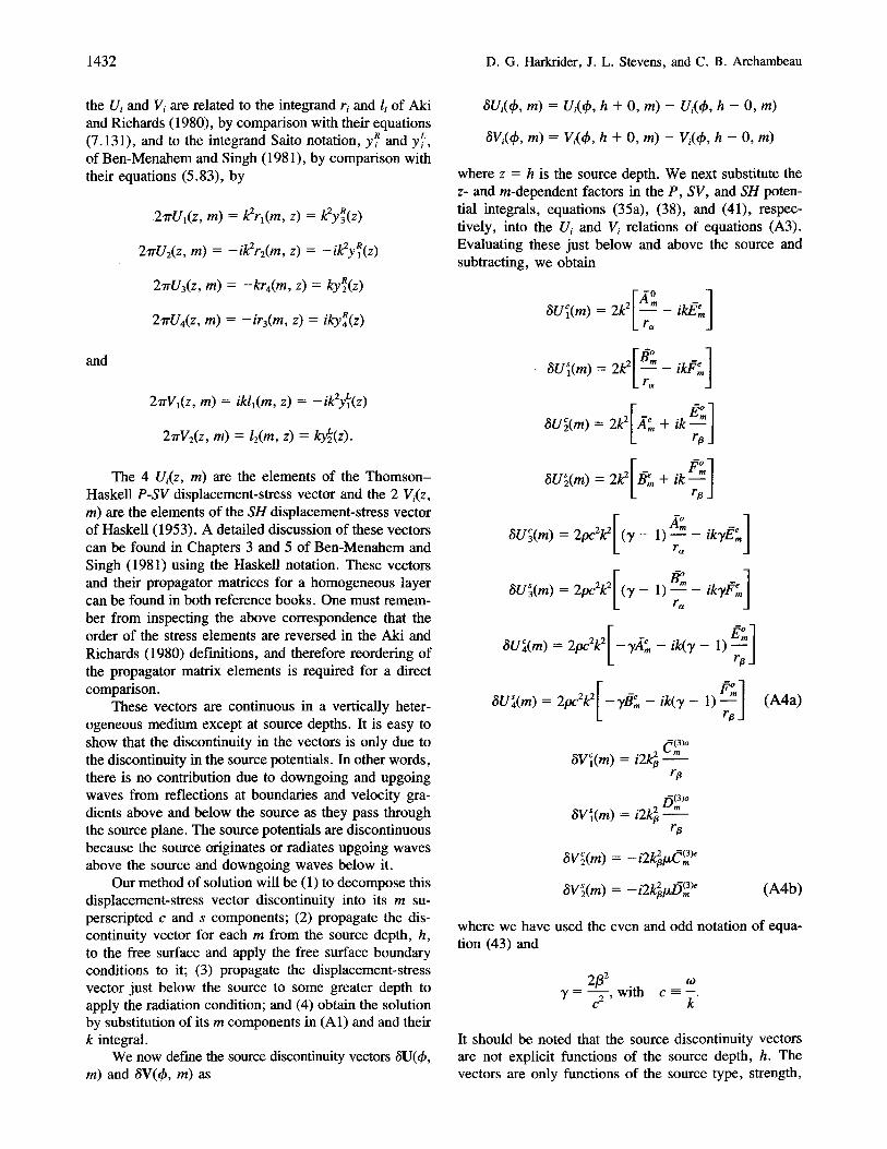
1432 D.G. Harkrider, J. L. Stevens, and C. B. Archambeau
the U,- and V~ are related to the integrand r~ and l; of Aki and Richards (1980), by comparison with their equations (7.131), and to the integrand Saito notation, y~ and y~, of Ben-Menahem and Singh (1981), by comparison with their equations (5.83), by
27rUl(z, m) = ~r l (m , z) = ~y~(z)
27rUz(z, m) = -ik2r2(m, z) = -ik2y~(z)
2zrU3(z, m) = -kr4(m, z) = ky~(z)
27rU4(z, m) = - i r3(m, z) = iky~(z)
and
27rVl(z, m) = ikll(m, z) = - i k 2 ~ ( z )
27rV2(z, m) = 12(m, z) = ky~2(z).
The 4 Ui(z, m) are the elements of the Thomson- Haskell P-SV displacement-stress vector and the 2 V~(z, m) are the elements of the SH displacement-stress vector of Haskell (1953). A detailed discussion of these vectors can be found in Chapters 3 and 5 of Ben-Menahem and Singh (1981) using the Haskell notation. These vectors and their propagator matrices for a homogeneous layer can be found in both reference books. One must remem- ber from inspecting the above correspondence that the order of the stress elements are reversed in the Aki and Richards (1980) definitions, and therefore reordering of the propagator matrix elements is required for a direct comparison.
These vectors are continuous in a vertically heter- ogeneous medium except at source depths. It is easy to show that the discontinuity in the vectors is only due to the discontinuity in the source potentials. In other words, there is no contribution due to downgoing and upgoing waves from reflections at boundaries and velocity gra- dients above and below the source as they pass through the source plane. The source potentials are discontinuous because the source originates or radiates upgoing waves above the source and downgoing waves below it.
Our method of solution will be (1) to decompose this displacement-stress vector discontinuity into its m su- perscripted c and s components; (2) propagate the dis- continuity vector for each m from the source depth, h, to the free surface and apply the free surface boundary conditions to it; (3) propagate the displacement-stress vector just below the source to some greater depth to apply the radiation condition; and (4) obtain the solution by substitution of its m components in (A1) and and their k integral.
We now define the source discontinuity vectors 6U(th, m) and 6V(~b, m) as
6Ui(q~, m) = Ui(qb, h + O, m) - Ui(#b, h - O, m)
6V~(qb, m) = Vi(q~, h + O, m) - V~(qb, h - O, m)
where z = h is the source depth. We next substitute the z- and m-dependent factors in the P, SV, and SH poten- tial integrals, equations (35a), (38), and (41), respec- tively, into the Ui and V~ relations of equations (A3). Evaluating these just below and above the source and subtracting, we obtain
6U~l(m) = 2k 2 .*m _ ikff,~ Lr~
I ] ~U~l(m) = 2 ~ - i ~ ;
~U;(m) = 2k 2 ,~e + i k - " rt3_l
6U~2(m) = 2k2[/~e + ik p ° ] r~_l
6U~(m) = 2pc2kZ[(-y - 1)Ar°--r~ - ikTff~e ]
6U~(m) = 2 p c 2 ~ [ ( 7 - 1) B~°-r~ - ikyf~.]
,U](m) = 2 p c Z k 2 [ - 7 , ~ e - i k ( 7 - 1)/~°] rt3_l
6U~4(m) = 2pc2k2[-71~e - ik(7 - 1 ) I~°1 (A4a) rt3J
°
6V~l(m) = i 2 ~ - 1 9
ro
/~(3)o = i 2 ~ - - " 6Wl(m)
r~
~Vg(m) = - i Z k 2 ~ C ~ )e
6V~(m) = - i 2 ~ / 5 ~ )e (A4b)
where we have used the even and odd notation of equa- tion (43) and
2fl 2 tO 7 = i with C--------.
C 2 ' k
It should be noted that the source discontinuity vectors are not explicit functions of the source depth, h. The vectors are only functions of the source type, strength,

Theoretical Rayleigh and Love Waves from an Explosion 1433
and the density and elastic parameters at that depth. This is the reason that we did not write them as a function of h.
From this point on, we restrict our development to the P-SV system and drop the ~b and m notation, while remembering that the following is for each coefficient of sin (mth) and cos (mth).
In order to apply a free surface or ocean bottom boundary condition, we relate the P-SV source discon- tinuity vector with the surface or the top of the solid half- space, z = 0, using the 4 × 4 P-SV propagator matrix, AR(z2, zl), where
U(z2) = AR(Z2, Zl)U(zl) .
It should also be noted that the R and L subscripts in- dicate Rayleigh and Love waves, respectively, since that is how the propagator matrix was originally used in seis- mology even though its use now includes the complete P-SV and SH solutions. Since our derivation will only use the propagator from the surface, z = 0, to depths, z, we use the shorthand AR(z) and A~s for Ag(h).
We can now write
U(h - 0) = ARsU(0),
relating the vector above the source to the surface ele- ments U(0). Defining a new vector G as
G = A~ -1 U(h + 0),
where the superscript - 1 indicates the matrix inverse, and substituting the two relations into the vector discon- tinuity definition above, we have
U(O) = G - AR~ 6U.
The z-dependent parts of the displacement solutions are the first two elements of U(0) and we see that G rep- resents the homogeneous, i .e., no source or 6U = 0, part of the solution. The second term in the expression rep- resents the inhomogeneous part, which propagates the source strength to the surface.
Our boundary condition is that the surface shear stress vanish, which requires U4(0) = 0, and that the normal stress either vanish or be equal to the negative of the fluid pressure above the interface. This requires that U3(0) = 0 or in the fluid case that the ratio of pressure to ver- tical velocity be known. The value of this ratio has been given in the literature for oceans and even atmospheres since the early years of matrix methods in seismology (e.g., Haskell, 1953; Harkrider and Flinn, 1970; etc., and see also Ben-Menahem and Singh, 1981, Section 9.7). We will present this ratio here in symbolic form as P0 and remark that it is only a function of the thick- ness and physical parameters associated with the fluid
and, of course, (o~, k). We write this boundary condition as
u~(o) = P o U @ ) .
Substituting these boundary conditions in the above, we have
UI(0 ) = G, - (A~))~j6U:
U2(0) = G2 - (A~sl)2j6Uj
PoU2(O) = G3 - (AR~)3j6U:
0 = 6 4 - (AR1)4j~Uj. ( A 5 )
In order to determine G1 and G2, we propagate the displacement-stress vector just below the source to a depth, D, where we apply the radiation condition. The main criterion for choosing D is that it be deep enough for all waves of interest and their structure interactions to have taken place well above D. In practice, this choice is very subjective and depends on frequency and range. Thus, at depth D,
U(D) = AR(D, h)U(h + 0),
and from the definition of G, we obtain
U(D) = AR(D, h)AR(h)G
or
U(D) = AR(D)G.
This last results from the multiplication property of prop- agator matrices. AI~ this point, we assume that we have a homogeneous half-space below this depth and there- fore can convert our dispacement-stress vector to the P-SV potential vector, P(z). This vector contains the coeffi- cients of the potential terms associated with P and SV waves in homogeneous regions of the half-space and is given at depth D by
P(D) = (A", ¢o", A', ¢o') r,
where the superscript T denotes transpose. The P and SV potentials can represent either propagating or exponen- tial waves in the z ,direction, depending on the values of (w, k). The terms A" and w" are the coefficients of the upgoing or exponentially growing P and SV waves, re- spectively. The terms A' and oJ' are the corresponding coefficients for the downgoing or exponentially decreas- ing waves with increasing depth.
Depending on the ~,alues of (w, k), our radiation boundary conditions are that UI and U2 ~ 0 as z ~ oo

1434 D .G . Harkrider, J. L. Stevens, and C. B. Archambeau
or that there be no upgoing waves below that depth. Both conditions can be accomplished by the requirement that A" and to" be zero, or
P(D) = (0, 0, A', to') r.
Now the potential vector and the displacement-stress vector are related by
P(D) = T -1 U(D)
where the T -1 matrix is given in Harkrider (1970). The matrix can also be obtained from the E -1 matrix of Has- kell (1953) and Ben-Menahem and Singh (1981), equa- tion (3.184), since it similarly relates the displacement- stress vector to the potential coefficient vector by
(A' + A", A' - A", ~o' - to", to' + to") r = E-1 U(D).
Substituting from above, we have
P(D) = R G, (A6)
where we have defined the R matrix by
R = T - 1 AR(D) .
When discussing multilayered media, Ben-Menahem and Singh (1981) define and frequently use the following scalars, which can be written in terms of R as
L = R l l , K = Rip_ , G = R13, R = R14 , N = R21 ,
M = R22, H = R23, and S = R24.
We now apply our radiation boundary condition and ob- tain from the first two elements of equation (A6),
which yield
0 = R l j G i
0 = R2jGj
R14G 3 + R15G 4 G1 =
Rll
(A7)
R12G3 + RI3G4 G 2 = , (A8)
Rll
where R is the 6 × 6 sec compound matrix of R formed by its minors, defined here as
where s = 1, 2, 3, 4, 5, 6 corresponds to pairs jk = 12, 13, 14, 23, 24, 34 with an identical correspondence of t to lm (Gilbert and Backus, 1966; Thrower, 1965). The
/ - 1 \
R(~m K) notation is from Dunkin (1965). In the R nota- \ - - !
tion, we also have the following commonly used quan- tities in Ben-Menahem and Singh (1981):
N K - L M = - R l l
G N - H L = -R12
R N - S L = -R13
G M - H K = - R 1 4 .
Before going on, we should discuss the homoge- neous contribution of G. From above, we see that G can be propagated continuously all the way from the surface down to the bottom, where we force it to satisfy the ra- diation boundary condition. We also see from equation (A5) that it does not satisfy the surface boundary con- ditions unless there is no source, i .e., 6U = 0. Then G 3
and G4 satisfy the traction boundary condition at the sur- face. Let us look at equations (A8) when G 4 = 0 and define the following "homogeneous" quantities, which we will denote with an H subscript:
[U o ] io ] R14 H H R12
o r
[U~oo] -- H R12 R13 (A9)
since it can be shown that R I 3 = R I 4 using properties of
Into] the propagator matrix inverse. Since is a pure H
imaginary number, it is frequently referred to as the Rayleigh wave "ellipticity." We also define
. 1 [Po]n -- - . (A 10)
H R 1 2
For the set of (o~, k) for which Rll is zero, we see that G 3 is zero, and we satisfy a free surface boundary con- dition since G4 was also set to zero in order to obtain the ratios. Under these conditions, we cannot use equa- tions (A8) to obtain the ratio G 1/G 2 . But from equation (A7), we have

Theoretical Rayleigh and Love Waves from an Explosion 1435
GI RI2
G2 Ru
and with Ru = 0, or
R22 R12
R21 Rll
equation (A9) reduces to the free surface relation above. Thus, equation (A9) can be used whether or not there is a fluid above the solid surface.
With these definitions, we define the normalized ho- mogeneous P-SV vector and SH vector as
[U(z) / -= AR(z)(-R13/R~2, 1 -R1~/R12, 0) r (All) -1
U2(0)J~
and
V(z) ] ~ AL(z)(1 iFL/['L) ~, Vl(O)J,u
(A12)
where FL and fiL will be defined when we return to SH. The P-SV components are normalized by the homoge- neous vertical surface displacement and the SH com- ponents by their homogeneous surface displacement. The correspondence between this notation and the Yi notation of Saito (Saito, 1967; Takeuchi and Saito, 1972; Ben- Menahem and Singh, 1981, Ch. 2) and that of Haskell (Haskell, 1953, 1964; Harkrider, 1964, 1970; Ben-Men- ahem and Singh, 1981, Ch. 2, 3, and 5) for these nor- malized homogeneous displacement-stress vector com- ponents is
U2(0)JH L Wo JH
U2(0)JH L Wo JH
Uz(O)j u = kff~(z) = kWo/Cl"
V4(z) U:(O)J,~ I Wo/C JH
(A13)
[v,(z, 1 F*)l Vl(0)JH = y~(z) = L Vo _1~
Vz(z)] i [zL(z)] gl (0)J H = k yL(Z) = Lifo~CAn
(A14)
where
Yc / c = ikx
and the bar or Yi(z) denotes that the yi(z) are normalized by their respective yl(0).
The homogeneous vectors satisfy the boundary con- ditions at depth and are continuous across the source depth but do not satisfy the surface boundary conditions for all (w, k). In particular, we see from equation (All) that the P-SV vector only satisfies the normal stress boundary condition for the set of (w, k) which yield a value of the ratio, -Ru/R12 equal to P0 or zero, i.e., Rll = 0, if the boundary is a free surface. For a given w, we denote this wavenumber as the Rayleigh-wave eigenvalue, kR, and its associated normalized homogeneous vector as the Rayleigh-wave eigenvector. From inspection of equation (A12), the SH vector will only satisfy the vanishing of its associated surface shear stress when FL = 0. This Love-wave eigenvalue is denoted as kL and its normal- ized homogeneous vector as the Love-wave eigenvector. When written out in scalar form for these eigenvalues, the relations (All) and (A12) correspond to equations (5.130) in Ben-Menahem and Singh (1981) with Rll = 0, since their relations are for a free surface.
We are now ready to proceed. Our final step is to substitute equations (A8) into the integrands of the sur- face displacements, i.e., the first two relations of equa- tions (A5), using the values of G3 and G4 given by the last two relations of equations (A5). Substituting U2(0) into equation (A1), we then obtain as our integral so- lution for the vertical displacement at the surface of our vertically inhomogeneous half-space
Wo = E m=O
Rll[Alm + R12[nlm + RI364(~, m)
Fe J,.(kr)dk
(A15)
where
Fe = Ru - PoR12
and the numerator definitions are
[A]m ~ -(ARs)43~UI( ff) , In) + (ARs)33~U2( ff), In)
- (Ags)236U3(qb, m) + (Ags)136U4(qb, m)

1436 D.G. Harkrider, J. L. Stevens, and C. B. Archambeau
[B]m ~- (ARs)42~Ul(6, m) - (ARs)32~U2(6, m)
+ (ARs)EE6U3(q~, m) - (ARs)12~U4((~ , m)
G4(~b , m) = - - ( A R s ) 4 1 ~ U I ( ~ ) , m) + (ARs)31~U2(I~), m)
-- (ARs)21aU3(~, m) + (ARs)ll~U4((~, m).
In the numerator, we have replaced the elements of the inverse propagator matrix with elements of the propa- gator matrix itself using the relation
(A-1)jk = ( - 1)J+~(A)o
w h e r e l = n + 1 - k , p = n + 1 - j , a n d A i s a n n x n matrix (Harkrider, 1964; Menke, 1979).
Equation (A15) was presented by Wang and Herr- mann (1980) in terms of Dunkin's (1965) notation. As in Haskell (1964), they left the numerator in terms of the propagator matrix from the source to the surface. Re- placing elements of the propagator matrix with those of its inverse, i.e., the propagator matrix from the surface down to the source, we are able to obtain the solution in a more concise form. Collecting the terms in the nu- merator and using the definition of the normalized ho- mogeneous vector elements (A11) and their relation to the Saito (1967) notation (A13), we have
1~ o = ~'~ - - (~Ul(~b , m)y~(h) m=O J 0
- - 6U2(6, m)ffl~(h) + 3U3(6, m)2f~(h)
_ i~U4(q~, m)y~(h) ~ R12 J "-V-[e Sm(kr)ak. (A16)
Using similar steps, we find that the surface azi- muthal displacement due to SH waves is given by
Vo = m=0 ,10 ~ ~ l )71(h)6V2(~b' m)
dJ,.(kr) y~(h)6Vl(qb' m) d(kr) dk (A17).
where
PL (AD22 * * = - (AL)lZtztrtj l
EL = - (AD~' , - (AD11mr~l
(AD =- (&(D))
and
X = / X * .
The only restriction on this form of the integral so- lutions is that at some depth the media is terminated by a homogeneous half-space commencing at depth D and the half-space variables are subscripted 1.
Evaluating the residue contributions of displacement solutions, (A16) and (A17), in order to obtain the sur- face displacements due to Rayleigh and Love waves, re- spectively, yields
7r E -6U,(~b, m) fiR(h) {rPo}~ = i ~ ARm=o
i - 6U:(dp, m) ~ y-R(h) + 6U3(qb, rn)y~(h)
- i~U4(q~, m)ff~(h)}. H~)(kRr)
(A18)
1 R 0 {qo}. = y 3 ( o ) (A19)
where
R~ A ~ R - -
or equivalently in terms of energy integrals
1 A R - - - -
2CRURII~
where
f 0 °¢
I R = p{LYlR(Z)] 2 + ~(z)]Z}dz
with the notation and

Theoretical Rayleigh and Love Waves from an Explosion 1437
n{ {Vo}L = --i ~ AL = 8V2(4,, m)y}(h)
i -L ] dH~) - 6V,(4, ,m)~y2(h)~---~rr(kLr ) (A20)
where
1 At =
/OFL\ ( A L ) ' 1 ~ - ' ~ ' - ) ~ °
o r
1 A L ~ m
2CLUL IL
where
/ '~ = plykz)l~dz.
Since the Rayleigh-wave eigenvalues are the kR for a given to which yield zero denominators for integral representation, equation (A16), we have from Fe = 0 that P0 = -Rn/R~2. And thus, the elements of the nor- realized homogeneous vector of (A11) in the numerator of the Rayleigh-wave contribution satisfy all the surface boundary conditions and are indeed eigenvectors. Sim- ilarly for the Love-wave homogeneous normalized vec- tor of equation (A 12), since for the residue contribution of equation (A17), FL = O.
Appendix B Cylindrical SV Potential Coefficients in Terms of
Cartesian Shear Potential Coefficients
The vertical displacement integrand, w, of its k in- tegral is related to the compressional and Cartesian SV potential integrands by
0 ( I ) OxIt 2 OXI-¢ l W = - - + - -
Oz Ox Oy
and in terms of the compressional and SV potential in- tegrands by
w = - - + k2XI , ' 0z
1(0. 0.,] 7y:
In terms of cylindrical coordinate derivatives
/?xI, = [cos 4' - - 0~tt 2 sin 4, 0~2
Or r 04,
cos 4, 0 . , ] sin 4,
ar r a4, J
where the Cartesian potential integrands are
n
~1 = i Z [--m(~(1) COS m4, + /5~ ) sin m4,]JmF# m=O
n
= Z --~(2) /5~ ) sin m4,]JmF a ~2 i lCm costa4, + m=O
o r
k~ = i ) cos 4, cos m4, + --m/~(2) COS 4, sin m4, m=0 t .
dJm C.) sin 4, cos m4, - / 5 ~ ) sin 4, sin m4,] ~rr
+ [C~ ) sin 4, sin m4, - / 5 ~ ) sin 4, cos m4,
'-1 + C~ ) cos 4, sin m4, - / 5 ~ ) cos 4, cos m4,]m ~ F¢
and
dJm
d(kr) - 1/2(Jm-~ - J,.+O
& m - = 1/2(J,n-1 + J,,,+l)
kr
which by inspection yields the relation then

1438
{2o 2 k ~ = i [1~'~ ) cos (m - 1)~ +/5(2) sin (m - 1)~
=m sin (m 1)4, - ~m -- + C m _ -~(1) COS (m 1)q~]J,n-1
.m(2) C O S ]~ (2 ) + [ - c , . (m + 1)~b - --m sin (m + 1)th
+ C(~ ) sin (m + 1)~b
(m + 1)~b] Jm+l}Ft~. • ,--':-- ( 1 ) - - L I m C O S
Collecting and identifying with
n
xlt = i E ( /~ cos m~b + if,, sin m~b)J,,,Ft3. m = 0
We have the following recurrence relation
- 2 ) 7 . (2 ) .'1 / / ~ ( 1 ) "F /-~(1) "1 2kff, m (tiT'(m2 + 1 = - - { J m - l l - - \ l J m + 1 ~ m - I !
- - 1) - - ( 2 ) 2kF,. = (C(~+1 + C'(1)-I) + (D,.+~ - /5~)_,) 1 __-< m -<_ n
where C~ ~ and/5~) are zero for m > n and m < 0 and
and
~o(2) ,~,(1) ~!1) 1~(2) = O o a n d o = - - ~ o
;o=0
As an example, when n = 6, we have
2kEo = C{ 2) - 15{ 1)
2k/~1 = C(22) -/5(31) _ 2g(o 2)
2k/~2 = C~ 2) -/5(31) - C{ 2) -/5{1)
2k/~3 = C(42) - / 5 ? ) - C(22) -/5(2 L)
2k/~4 = C(52) - - / 5 ( 1 ) __ ~(32) _ /5~1)
2/cE s = -(7(42) -/5(41)
2 k / ~ = _~2 ) - - /5~1)
2 k ; o = o
2k/~ 1 = QI) +/5(22) + 2C(1)
2kff2 = C~1) + ]5(32) + C-~1) _ ]5(12)
D. G. Harkrider, J. L. Stevens, and C. B. Archambeau
2kff3 = C (I) --I- L~{4 2) -]- C O l) - D(2 2)
2kff4 = (~1) +/5~2) + C(31) _ ]5(32)
2kFs = +(7? ) - 15(42)
2kff 6 = +g~5 z) -/5~')
Appendix C Cartesian and Cylindrical Multipole Coefficients for Quadrupole Sources of Arbitrary Orientation
Comparing Harkrider (1976) equations (A8) with this article's equations (33), we obtain the following Carte- sian coefficients:
A20 = - K ~ sin A sin 28
2 A21 = 3 Kak2" cos A cos 8
1 Az2 = - g K ~ sin a sin 28
Kt3 ~ sin )t cos c(l) 28 20 =
1 K ~ sin A sin 28 = - - _ D~z11~ 3
1 D(1) = Kt3 ~ cos A cos 8 22 ]~
1 C(3] ) = g Kt3 ~ sin A sin 28
1 C(2) Kt~ ~ cos A cos 8 22 - -
12
1 Kt3~ sin A cos 28 C(3]) 6
,-<3) 1 = --x g L'22 6 COS A sin 8
B21 = - ~ K ~ sin h cos 28
1 BEE = --3 K , ~ cos A sin 8
1 K ~ cos A sin 6 c(,1, =

Theoretical Rayleigh and Love Waves from an Explosion 1439
C(o - 1 K ~ sin A cos 26 22 - -
C(2) = 1 ~o ~ / c ~ g cos ~ cos 6
1 D<2] ) = --~ KI3/~ ~ cos A sin 6
0
1 D(Z) = K ~ sin A cos 26 22
1 K~/fl~ cos A cos 6 D?; = -;
1 D(3) = gtl]~ ~ sin A sin 26. (C 1) 22
The resultant cylindrical coefficients using Appendix B a r e
1 Ar~ = ~ K,,(k 2 + 2 ~ ) sin A sin 26
2tc~
1 Ar~ = ~ K~k 2 sin h sin 26
2 ~
2 Ar~ = --;S K~kp~ cos A cos 8
k~ 1
B~~ = _--z K ~ cos h sin 6 X;
2 B~ = 7z K~kv~ sin A cos 26
3 £ ; = k--;S,a Kt3vt3 sin A sin 26
ztct3
1 / ~ = 2 "~K~ Kav~ sin A sin 26
1 (/,.~ - 2k 2) /~ = ~ Ks k cos ~, cos 6
1 C] 3)° - , ~ Kt3kvt~ sin A cos 26
1 C? )e = - ~ K~k 2 cos A sin 6
1 :~ = ;S K~v~ cos h sin 6
ks
1 2/fl) sin A cos 26
1 b~ 3)° - . , K~k~,~ cos ,~ cos 6
,c~
1 /5~ 3)~ = ~ KCk 2 sin A sin 26 (C2)
z~
A p p e n d i x D C a r t e s i a n and C y l i n d r i c a l M u l t i p o l e C o e f f i c i e n t s
fo r a S e i s m i c M o m e n t T e n s o r
The definition of the second-order seismic momen t tensor is
0 ui(x , t) = Mpq * ~ Gip
OCq
Ui(X , t) = -Mpq * aip,q
o r
a~(x, oo) = - ~('°)c~. " ' ~ p q v z p , q ,
where the c o m m a denotes differentiation with respect to the observer coordinates, x, rather than the source co- ordinates, ~.
Now
aipq- l ( 03 O A } • 4 7 r p o 9 2 OxiO;Oxq(Afl-A°t)~-k2~iP~xq O"
N o w f rom equations (25), we have that
1 0 ~ i 4,-
Oxi
and
1 oak
o r
1 ~ = --~ MpqGip,qi
and

1440 D.G. Harkrider, J. L. Stevens, and C. B. Archambeau
02 02 02 } Gip qi = 1 0 OXqO3f, i ' 4rrpto 2 x-~Xq 3x2i (A~ - A~) + ~ i p ~ Aa
and since
02 0 2 02 A~=-k2~A~ and 3 ; p - - A a = - A a
dX i OXqdX i OXqdXp
we have
1 02 ' 4"/rpo92 OXpOXq A~.
Thus
~ = 1 _ 0 2
47rpt° 2 Mpq OXpOXq A~
02 02 02 1 / ~ 1 1 - + ~ / [ 2 2 - "1- 2 3 3 -
4,trp092 0x21 3x 22 ax E
0 2 + 2 / ~ 1 2 -
Ox~Ox2
+ 2213 ~ + 2M23 A~. Ox~Ox3
From Erd61yi (1937)
h~n2)(k~R)p~n (cos O)e ime~ = i-"(D~)me~nm)( o / Oik~z)h~o2)(k~R)
(D1)
where the differential operator D~ is defined as
D ~ - - - - + i . ik~
Combining equation (D1) with
i ( 3 02A~ ) h(22)(k~R)P(2°)(cos O) = K \ ~ 3~ + A~
and
(2) k A~ = -ik~ho (~R).
We have
0% ~ 2 Ox 2 = i 3 {h~ ) (k~R) - 2h~22)(k~R)/~2(cos 0)}
Ox-~l - i h~oZ)(k~R) + h~EE)(k,,R) P°(cos 0)
1 pE(cos O)cos 2~b]} 2
0% . k~ { Ox 2 - t-~ h(02)(k~R) + h(22)(k~R)
"[P°(cosO)+~p2(cosO)cos2d~]}
- - = -- i - - h 2 (kvg)P2(cos 0) sin 2th OXlOX2 6
= - i -- h~22)(k~R)pl(cos O) cos ~b OxiOx3 3
O~A~ OX20X 3 - - = - i -- ~ h(22)(k~R)P~(cos O) sin ~b.
3
Comparing with the definition of the Cartesian multipole coefficients, we have
1 k 5 Aoo - - - ' (/~11 -~- M22 "~-/~33) 47rptO 2 l "~"
and
A2o- 47rpt° 2 i ~ (/~ll -~- /~22 -- 2/~33)
A21 = + _~1__ 2i~2M13 47rpto 3
" ~ - 222) A22 = +47rpto 2/ 6 (M~I-
B21 = q------~l i k5a 2/~23 4qrpto 2 3
B22 = + i - - (D2) 4"ffptO 2 3 MI2"
Now
0 4 eok xjO-- = -2pqeoA. ,~
and

Theoretical Rayleigh and Love Waves from an Explosion 1441
akp qj : 1 { 02 02
" 4=p,, , 2 oxTOxq ox~o--7, ~A~ - Ao~
~2
+ Sake ~ A ,} .
Operating with euk, the first term is zero since it is sym- metric in (j , k), and
_ 1 2 02 eo~Gkp,q j - 4 7r-~w 2 kt~eijp ~ AtJ OXqOXj
thus
1 02 @i -- eijpMpq - - Ae,
47rpw 2 OXqOXj
which yields
~- . . . . q- /~23 47rpw2 (M33 11422) Ox20x3
o 2 ) - o ~ 0 ~ } M13 OXlaX2 oxTx 3
~X 2 + a7112 A ~
~t 2 1 { (/~11 /~33) 02 - ( 02 . . . . -{.- M13
47rP t O 2 0 X l O X 3 "~3
"~ /~12 - - -- /~23 Ae OXzOX 3
. . . . q- M12 4 ,B.p (.o 2 (/~22 /~11) OxlOx2
-}- /~23 - - -- /~13 A/3. Ox~ Ox3
Comparing as before, we have
1 C( 1 ) __ iksgJ~23
20 87TpO) 2
k 5 i ~ /~12 C~ll ) = 8 ~pto2 3
D~l~ ) = - - - 1 •/4
l (/~22 -- /~33) 87rpto2 3-
C ( 1 ) _ 1 . / ~ _ 2 2 8qTptO--" ~ l 6 M23
n m 1 k 5 - - J3 - • --22 = +8~.p~o 2 i ~M13
1 C(2) = - - i ~/~13
20 + 8~pto2
1 k s _ C~22~ = +8rrpw------- ~ i 3 (Mll - )Q33)
1 5 - D~2] ) = +87rpto--------- 5 i 3 MI2
,-,{2) 1 k 5 • ~2z = 8rrpw2 i -ff M13
k 5 _ r~(2) __ 1 ~'/3 1/22 8 ,././.p (.02 i M23
C(3) = 0 20
1 5 - C~2] ) = +87rpw------- 5 i -~- M23
o~]' - 1 ~ _ 87rpw-------- 2 i ~ M13
c.(3) 1 k 5 • ~2z = +87rpw2 i ~- M12
D(3) _ 1 i ~ 22 8.ffpo)2 -6- (/~11 -- M~2)- (D3)
The resulting cylindrical coefficients, using Appendix B, are
" ~ o = q . m 1 i
47rpto 2 2 [k2(]klll + / ~ 2 2 ) + 2M33(k2a - k2)]
1 X 1 - - 2ek~5~13
= + 47rpto 2
1 i A 2 = -~ - - k2(/~22 - Ml l )
4~rpto 2 2
1 - - 2 e k ~ 2 3
]~1 = +4,rrptoZ
1 /~2 - - - i k2/~12
4 rrpo 2
C~ ) = 0
1 C~ 3) - 41rpto 2 ekvt~M23

1442 D . G . Harkrider, J. L. Stevens, and C. B. Archambeau
and
i - - k2/~l 2 0(23) = +4~p¢02
1 D~ 3) +47rptoz
i 87rptO 2 k2(Mll -
1 /~0 -- ~5~ .pO)2 {/~fl(/~ll ~- /~22 -- 2M33)
/~, = i (2k 2 - ~ ) ~ , ,
47rpto 2 k
1 /~2 = +8,WpO)"--'- ~ •/~/3(/~II -- /~22)
ffl - i (2kZ - ~ ) M23 4"/rpto 2 k
(D4)
1 F2 = +4rrpto--'-- S •~/~12
where
• = s g n ( z - h ) .
Thus, coefficients involving • are odd and the other coefficients are even, in the sense of equations (42).
Seismological Laboratory California Institute of Technology Pasadena, Califomia 91125
(D.G.H.)
S-Cubed, Division of Maxwell Laboratories, Inc. La Jolla, California 92038-1620
(J.L.S.)
Physics Department University of Colorado Boulder, Colorado 80309
(C.B.A.)
Manuscript received 12 February 1990.