München

Ludwig

UniversitätMaximilians

Theoretical Description of Angle ResolvedPhotoemission in the X-ray Regime on the Basis

of the One-Step Model

H. Ebert, J. Minar and J. Braun

Department Chemie und Biochemie,

Physikalische Chemie, Universitat Munchen, Germany

In collaboration with:

N. Brookes - ESRF

C. Fadley - University of California Davis

C.M. Schneider - Research Center Jülich

haxpes09 – p.1/23

München

Ludwig

UniversitätMaximilians Outline

Introduction

Importance of surface contributions

One-step model of photo-emission

Reduction of surface sensitivityfor high photon energies (HAXPES)

HAXPES specific issuesphoton momentumthermal effectsnon-dipole contributions (not yet)

Summary

haxpes09 – p.2/23

München

Ludwig

UniversitätMaximilians Description of PES via three-step model

three-step model of photo-emission (ARPES)Berglund and Spicer (1964)

I

III

IIIII Escape to the vacuum D(E,ω)

II Transmission to surface T (E,~k)

I Excitation 〈n′~k|~p|n~k〉

I ∼ D(E, ω)∑

nn′

∫d3k T (E,~k) |〈n′~k|~p|n~k〉|2

×δ(E − En~k

− ω)δ(En′~k

− E)Θ(E − EF )Θ(EF + ω − E)

haxpes09 – p.3/23

München

Ludwig

UniversitätMaximilians PES calculations based on three-step model

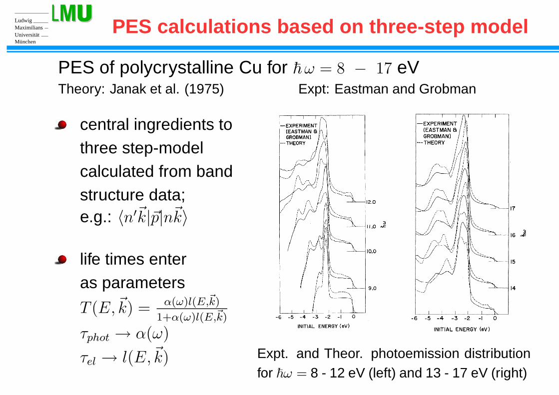
PES of polycrystalline Cu for ~ ω = 8 − 17 eVTheory: Janak et al. (1975) Expt: Eastman and Grobman

central ingredients tothree step-modelcalculated from bandstructure data;e.g.: 〈n′~k|~p|n~k〉

life times enteras parameters

T (E,~k) = α(ω)l(E,~k)

1+α(ω)l(E,~k)

τphot → α(ω)

τel → l(E,~k) Expt. and Theor. photoemission distributionfor ~ω = 8 - 12 eV (left) and 13 - 17 eV (right)

haxpes09 – p.4/23

München

Ludwig

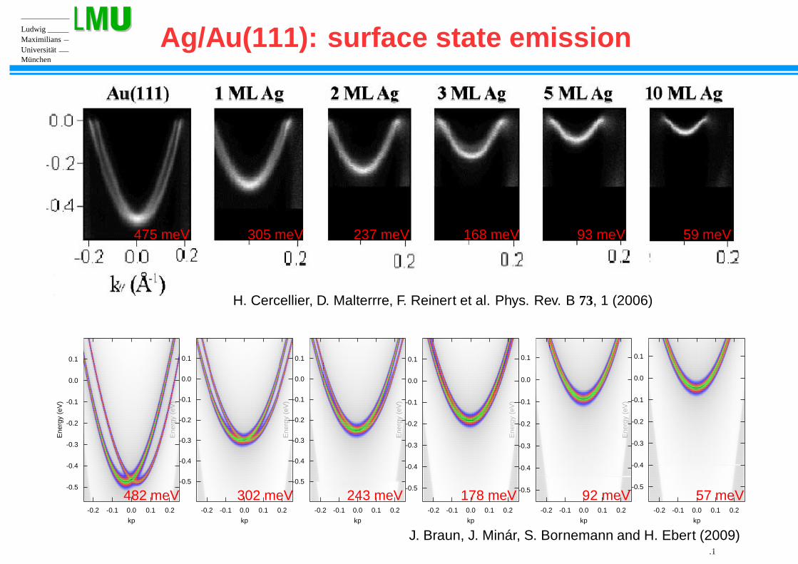
UniversitätMaximilians Ag/Au(111): surface state emission

475 meV 305 meV 237 meV 168 meV 93 meV 59 meV

kp

Ene

rgy

(eV

)

0.20.10.0-0.1-0.2

0.1

0.0

-0.1

-0.2

-0.3

-0.4

-0.5

kpE

nerg

y (e

V)

0.20.10.0-0.1-0.2

0.1

0.0

-0.1

-0.2

-0.3

-0.4

-0.5

kp

Ene

rgy

(eV

)

0.20.10.0-0.1-0.2

0.1

0.0

-0.1

-0.2

-0.3

-0.4

-0.5

kp

Ene

rgy

(eV

)

0.20.10.0-0.1-0.2

0.1

0.0

-0.1

-0.2

-0.3

-0.4

-0.5

kp

Ene

rgy

(eV

)

0.20.10.0-0.1-0.2

0.1

0.0

-0.1

-0.2

-0.3

-0.4

-0.5

kp

Ene

rgy

(eV

)

0.20.10.0-0.1-0.2

0.1

0.0

-0.1

-0.2

-0.3

-0.4

-0.5

482 meV 302 meV 243 meV 178 meV 92 meV 57 meV

H. Cercellier, D. Malterrre, F. Reinert et al. Phys. Rev. B 73, 1 (2006)

J. Braun, J. Minár, S. Bornemann and H. Ebert (2009).1haxpes09 – p.5/23

München

Ludwig

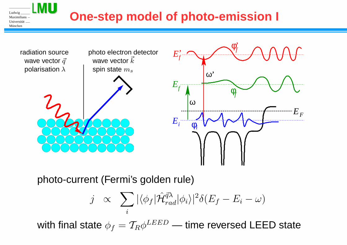
UniversitätMaximilians One-step model of photo-emission I

radiation sourcewave vector ~q

polarisation λ

photo electron detectorwave vector ~k

spin state ms

φ

’E

E

EEF

ii

f

ω

ω’

’φff

φf

photo-current (Fermi’s golden rule)

j ∝∑

i

|〈φf |H~qλrad|φi〉|

2δ(Ef − Ei − ω)

with final state φf = TRφLEED — time reversed LEED statehaxpes09 – p.6/23

München

Ludwig

UniversitätMaximilians One-step model of photoemission II

photo current

j ∝∑

i

〈φf |H~qλrad|φi〉〈φi|H

~qλ †rad |φf 〉 δ(Ef − Ei − ω)

∝ 〈φf |H~qλrad|Im Gi|H

~qλ †rad |φf 〉

initial state Green’s function

Im Gi(E) =∑

i

|φi〉〈φi| δ(E − Ei)

final stateφf = TRφLEED

= TR

[ei~kf~r +

∫d3r′G(~r, ~r ′, Ef ) V (~r ′) ei~kf~r ′

]

e.g. Caroli et al. (1973), Feibelmann and Eastman (1974)haxpes09 – p.7/23

München

Ludwig

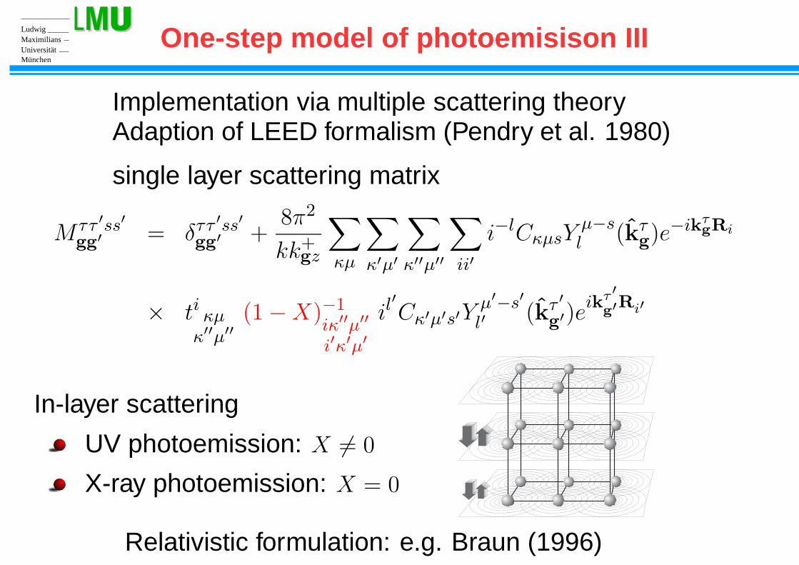
UniversitätMaximilians One-step model of photoemisison III

Implementation via multiple scattering theoryAdaption of LEED formalism (Pendry et al. 1980)

single layer scattering matrix

M ττ ′ss′

gg′ = δττ ′ss′

gg′ +8π2

kk+gz

∑

κµ

∑

κ′µ′

∑

κ′′µ′′

∑

ii′

i−lCκµsYµ−sl (kτ

g)e−ikτgRi

× ti κµ

κ′′µ′′

(1 − X)−1iκ′′µ′′

i′κ′µ′

il′

Cκ′µ′s′Yµ′−s′

l′(kτ ′

g′)eikτ ′

g′Ri′

In-layer scattering

UV photoemission: X 6= 0

X-ray photoemission: X = 0

Relativistic formulation: e.g. Braun (1996) haxpes09 – p.8/23

München

Ludwig

UniversitätMaximilians Surface sensitivity: nMgO/Fe(001) at 1000eV

calculated ARPES intensities I(E,Θ)

Fe(001) MgO

1 ML MgO/Fe(001) 8 ML MgO/Fe(001)

increasing

⇒coverlayerthickness

Fe-related features get lost with increasing MgO coverage haxpes09 – p.9/23

München

Ludwig

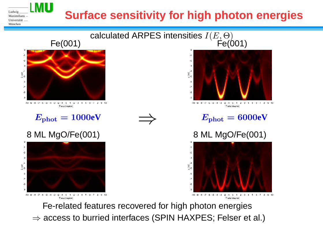
UniversitätMaximilians Surface sensitivity for high photon energies

calculated ARPES intensities I(E,Θ)Fe(001) Fe(001)

8 ML MgO/Fe(001) 8 ML MgO/Fe(001)

Ephot = 1000eV ⇒ Ephot = 6000eV

Fe-related features recovered for high photon energies⇒ access to burried interfaces (SPIN HAXPES; Felser et al.) haxpes09 – p.10/23

München

Ludwig

UniversitätMaximilians Photon momentum effects on Ag(001)

Ag(001) photoemission intensities along ΓK with LCP-light at hν=552 eV

A

-1.5 -1 -0.5 0 0.5 1 1.5

kparallel (A° -1)

-8

-7

-6

-5

-4

-3

-2

-1

0

Bin

ding

Ene

rgy

(eV

)

B

-1.5 -1 -0.5 0 0.5 1 1.5

kparallel (A° -1)

-8

-7

-6

-5

-4

-3

-2

-1

0

Bin

ding

Ene

rgy

(eV

)qphoton ignored

ki = (k|| + g,

√2(E − iVi1) − |k|| + g|2)

kf = (k|| + g,

√2(E + ω − iVi2) − |k|| + g|2)

qphoton included

ki = (k|| − q|| + g,

√2(E − iVi1) − |k|| − q|| + g|2)

kf = (k|| + g,

√2(E + ω − iVi2) − |k|| + g|2)

Venturini et al. PRB 77, 045126 (2008)haxpes09 – p.11/23

München

Ludwig

UniversitätMaximilians How to minimise photon momentum effects?

q = 0,Θ = 0 q 6= 0,Θ = 0

q = 0,Θ = 0.7 q 6= 0,Θ = 0.7

A

-1.5 -1 -0.5 0 0.5 1 1.5

kparallel (A° -1)

-8

-7

-6

-5

-4

-3

-2

-1

0

Bin

ding

Ene

rgy

(eV

)

B

-1.5 -1 -0.5 0 0.5 1 1.5

kparallel (A° -1)

-8

-7

-6

-5

-4

-3

-2

-1

0

Bin

ding

Ene

rgy

(eV

)

C

-1.5 -1 -0.5 0 0.5 1 1.5

kparallel (A° -1)

-8

-7

-6

-5

-4

-3

-2

-1

0

Bin

ding

Ene

rgy

(eV

)

D

-1.5 -1 -0.5 0 0.5 1 1.5

kparallel (A° -1)

-8

-7

-6

-5

-4

-3

-2

-1

0

Bin

ding

Ene

rgy

(eV

)

haxpes09 – p.12/23

München

Ludwig

UniversitätMaximilians Photon momentum effects on Ag(001)

Experiment Theory

Γ XX

-1.4 -1 -0.6 -0.2 0.2 0.6 1 1.4

kparallel (A° -1)

-8

-7

-6

-5

-4

-3

-2

-1

0

Bin

ding

Ene

rgy

(eV

)Γ XX

-1.4 -1 -0.6 -0.2 0.2 0.6 1 1.4

kparallel (A° -1)

-8

-7

-6

-5

-4

-3

-2

-1

0

Bin

ding

Ene

rgy

(eV

)

Γ KK

-1.5 -1 -0.5 0 0.5 1 1.5

kparallel (A° -1)

-8

-7

-6

-5

-4

-3

-2

-1

0

Bin

ding

Ene

rgy

(eV

)

Γ KK

-1.5 -1 -0.5 0 0.5 1 1.5

kparallel (A° -1)

-8

-7

-6

-5

-4

-3

-2

-1

0

Bin

ding

Ene

rgy

(eV

)

Venturini et al. PRB 77, 045126 (2008) haxpes09 – p.13/23

München

Ludwig

UniversitätMaximilians Thermal effects I

Thermal vibrations: fundamental limit to bandmapping as energy or temperature is raised

Superposition of direct and Non-direct transitions:

I(E, T ) = W (T )IDT (E) + (1 − W (T ))INDT (E)

Debye-Waller factor W (T ) ∝ exp(−∆k2〈u2〉T )

mean-square displacement 〈u2〉TShevchik (1977)

Experimental support:White and Fadley (1981)

T -dependent scattering matrix t withinLEED-formalism (Duke (1980))

t(T,~k,~k′) = t(0, ~k,~k′)W (T )haxpes09 – p.14/23

München

Ludwig

UniversitätMaximilians Thermal effects II

Based on Glaubert’s theorem (1955)

〈ei∆~k·~u〉T = e−1

2〈(∆~k·~u)2〉T

Transfer to 1-step model of PES and inclusion ofmatrix element effects: Larsson and Pendry (1981)

Forward focussing in VB-XPS:Osterwalder et al. (1990)

Improved treatment of phonon effects on LEEDstate - cluster implementation:Zampieri et al. (1996)

haxpes09 – p.15/23

München

Ludwig

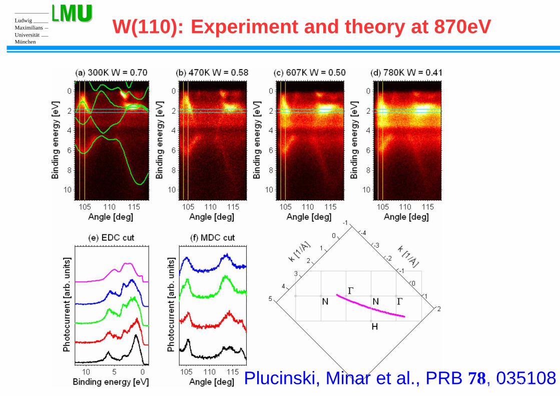
UniversitätMaximilians W(110): Experiment and theory at 870eV

Plucinski, Minar et al., PRB 78, 035108haxpes09 – p.16/23

München

Ludwig

UniversitätMaximilians W(110): Experiment and theory at 870eV

haxpes09 – p.17/23

München

Ludwig

UniversitätMaximilians W(110) at 5954eV, T = 30K

Experiment Theory (T=0K)

Theory, wide angular scan (T=0K)

haxpes09 – p.18/23

München

Ludwig

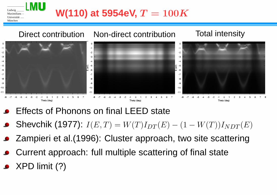
UniversitätMaximilians W(110) at 5954eV, T = 100K

Direct contribution Non-direct contribution Total intensity

Effects of Phonons on final LEED state

Shevchik (1977): I(E, T ) = W (T )IDT (E) − (1 − W (T ))INDT (E)

Zampieri et al.(1996): Cluster approach, two site scattering

Current approach: full multiple scattering of final state

XPD limit (?)

haxpes09 – p.19/23

München

Ludwig

UniversitätMaximilians Outlook: Electron-phonon interaction

Eliasberg function of Ni

0 10 20 30 40 ω [meV]

0

0.05

0.1

α2 F(ω

, kF)

[meV

]

Γ − L Spectral function for Ni (kink)

KKR Phonon calculations: linear response

Self energy Σel−ph(E,~k) =R

2ΣEi(E, ω)α2F (ω,~k)dω: A. Eiguren, C. Ambrosch-Draxl

include Σel−ph(E,~k) into KKR via Dyson Equation + Photoemission

calculations for complex systems and alloys (high-Tc-materials)haxpes09 – p.20/23

München

Ludwig

UniversitätMaximilians Outlook: effect of thermal vibrations in HAXPES

Scattering theory for dislocated atoms

vibrations of lattice sitesuncorrelated

assume dislocations ∆~Rn

to depend on temperature T

with probability P (∆~Rn, T )

average over dislocationsusing CPA alloy theoryP (∆~Rn, T ) ⇔ concentration

Combine with PES-theoryfor alloys (Durham)

+ + + + ++ + + + +

+ + + + ++ + + + +

. . . . .. . . . ...... . . . . .CPA averaging ⇓

+ ++ + +

+ + + + ++ + + + +

++ + +

+

leads to proper Green’sfunction without artefacts(Heiglotz)!

haxpes09 – p.21/23

München

Ludwig

UniversitätMaximilians Summary

Extension of the one-step model of photo-emission allowto deal with all aspects of HAXPES

photon momentum

thermal effectsmore refined models necessary

relativistic effects

matrix elements effects(magnetic) dichroismnon-dipole contributions

spin-resolution (SPIN-HAXPES)

haxpes09 – p.22/23

München

Ludwig

UniversitätMaximilians Munich SPR-KKR package

Forthcoming hands on course

KKR- hands on courseH. Ebert, W. M. Temmerman24.-26. June, Munich

see: http://olymp.cup.uni-muenchen.de/ak/ebert

haxpes09 – p.23/23