
Theoretical aspects of proton dosimetry
24
2 Theoretical aspects of proton dosimetry 2.1 Proton interaction with matter 2.1.1 Introduction For an understanding of the dose distribution produced by protons, a knowledge of their ener gy loss and scattering is needed. Protons traversing matter lose ener gy through successive collisions with the atoms and molecules of the material. With respect to ener gy loss, the most important interaction is between the proton and the atomic or molecular electrons. The interaction between a proton and an atomic nucleus effects the proton flux (nuclear reactions), and the proton trajectory ((in)elastic scattering). The most important parameter characterizing the ener gy loss of an incident proton is the stopping power, which is mean ener gy loss per unit path length in a material. A full description of the proton ener gy loss process, however, requires more detailed information than is provided by the stopping power alone. The amount of energy trans- ferred from a proton to an atomic electron, as well as the number of interactions that occur per unit path length has a probability distribution. This causes statistical fluctu- ations in the ener gy deposition. Moreover, there is a certain probability that very en- er getic electrons are produced (B-electrons or B-rays ) which can travel a considerable distance before their ener gy is deposited. The most important contribution to proton scattering comes from the electromag- netic interaction with the nucleus. This gives rise to small scattering angles, but since there are a lar ge number of collisions, the effect can be considerable. If the impact para- meter 1 is small also the hadronic interaction contributes to elastic scattering. In addi- tion inelastic interactions can occur: these can either be an inelastic scattering process during which the incident proton transfers ener gy to the nucleus (which will then be in an excited state and decay by -emission) or a nuclear reaction process (such as (p,n), (p,d), (p,2p) or (p,3p) ) where the incident proton will disappear. In case of scattering of protons by very light nuclei, such as protons in hydrogen, also the recoil nucleus can travel a considerable length before its ener gy is fully deposited. 1 distance of closest approach between proton and nucleus.
Transcript of Theoretical aspects of proton dosimetry
2
Theoretical aspects ofproton dosimetr y
2.1 Proton interaction with matter
2.1.1 Introduction
For an understandingof the dose distribution produced by protons, a knowledge of theirenergy loss and scattering is needed. Protons traversing matter lose energy throughsuccessive collisions with the atoms and molecules of the material. With respect toenergy loss, the most important interaction is between the proton and the atomic ormolecular electrons. The interaction between a proton and an atomic nucleus effectsthe proton flux (nuclear reactions), and the proton trajectory ((in)elastic scattering).
The most important parameter characterizing the energy loss of an incident protonis thestopping power, which is mean energy loss per unit path length in a material.A full description of the proton energy loss process, however, requires more detailedinformation than is provided by the stopping power alone. The amount of energy trans-ferred from a proton to an atomic electron, as well as the number of interactions thatoccur per unit path length has a probability distribution. This causes statistical fluctu-ations in the energy deposition. Moreover, there is a certain probability that very en-ergetic electrons are produced (B-electronsor B-rays) which can travel a considerabledistance before their energy is deposited.
The most important contribution to proton scattering comes from theelectromag-netic interactionwith the nucleus. Thisgives rise to small scattering angles, but sincethere are a large number of collisions, the effect can be considerable. If the impact para-meter1 is small also thehadronic interactioncontributes to elastic scattering. In addi-tion inelastic interactions can occur: these can either be an inelastic scattering processduring which the incident proton transfers energy to the nucleus (which will then be inan excited state and decay by ò-emission) or a nuclear reaction process (such as (p,n),(p,d), (p,2p) or (p,3p) ) where the incident proton will disappear. In case of scatteringof protons by very light nuclei, such as protons in hydrogen, also the recoil nucleuscan travel a considerable length before its energy is fully deposited.
1distance of closest approach betweenproton and nucleus.

30 Theoretical aspects of proton dosimetry
In the second part of this chapter the influence of the detection equipment on themeasured shape of the dose distribution is discussed. Because radiation detectors havea finite size, and have ingeneral a composition different from the medium one is in-terested in, they effect the outcome of the measurement. This is the subject ofcavity-chamber theory. This is especially important for the comparison of experimental datawith Monte Carlo calculations and for the determination of conversion factors betweendifferent detector types. Because protons can produce secondary particles (B-electrons,nuclear reaction products or recoil nuclei) as a result from energy loss processes therecan be a difference between the localenergy lossand theenergy absorbedby themedium. This also has consequences for the measurement of dose distributions.
2.1.2 Proton interaction with electrons I: ener gy loss
Within the energy range of importance in proton therapy (from stopping protons toä250 MeV) it is convenient to consider 2 energy intervals separately:
î Low energy: belowä0.5 MeV protons can pick up orbital electrons and form hy-drogen. Also energy can be lost to atomic nuclei due to electromagnetic interac-tions (nuclear stoppingpower). These are complicated processes, but fortunatelythey only play a role at the very last microns of a proton track. It is importantfor the subject ofmicrodosimetry, which deals with the energy loss process on amicroscopic scale (for example: the study of the effect of ionizing radiation onaAB). For our purpose (the macroscopic dosimetry of proton beams), however,its relevance is not so large so that we will not discuss it further.
î High energy: for proton energies betweenä 0.5 MeV and 250 MeV the atomsin the stopping medium can be excited or ionized . The collision process is wellunderstood and in principle the stopping power can be calculated theoretically.
The mean energy loss per proton7 can be described by theBethe theory[18] whichleads to the following expression:
�
47 ' ý�
4
_.
_5' g
~
ø
�
q2uEqä (2.1)
with:
g ' 2Zo2e6S2ù@ñ ä fé�DôD MeV cm2 g3� (2.2)
whereoe ' e2*eZ0f6S2 is the classical electron radius,0f the permittivity of the
vacuum (which is introduced by the use of SI units),6S2 is the electron rest massenergy, ù@ñ Avogadro’s number ,q is the particle velocity in units of the velocity of
light (q2 = � ýí
�S2
.n�S2
ì2),�S2 is the proton rest massä 938.3 MeV, . the proton
kinetic energy, ~ andø are the atomic number and relative atomic mass of the target

2.1 Proton interaction with matter 31
atom. The quantity uEqä takes into account the fine details of the energy loss processand is written as the sum of three terms:
uEqä ' ufEqä n u�Eqä n u2Eqä (2.3)
The first term isgiven by:
ufEqä ' *?
ë26S2q2A4@
�ý q2êý 2q2 ý 2 *? U ý 2
ä
~ý B (2.4)
whereU is theaverage excitation potentialof the atoms of the medium, C/Z theshellcorrection andB thedensity-effect correction. The shell correction plays a role at lowvelocities and deals with effects due to the finite speed of the proton compared to thevelocity of bound electrons. It can be as high as 10 % but is usually implicitly takeninto account by the choice of the excitation potentialU. The density correction takesthe polarization of the medium due to the passage of the projectile proton into account.It can be neglected for proton energies below 500 MeV (á fé� Iä. A4@ is the largestpossible energy loss in a single collision with a free electron,given by:
A4@ '26S2q2
�ý q2%� n
26
�s�ý q2
ní6�
ì2&3�(2.5)
whereS is the velocity of light,6 the electron mass and� the proton mass. The errorobtained by setting the factor between square brackets to 1 is smaller than 0.2 % forproton energies below 250 MeV. Theu�-term in equation (2.3) is known as theBarkascorrectionand is responsible for the slightly different stoppingpower for positively andnegatively charged particles. It does play a role at low energies, but is usually takentogether with the shell correction and implicitly included into the average excitationpotentialU. Theu2-term is known as theBloch correctionand only important forrelativistic energies. When one deals with a compound medium, which is usually thecase in proton therapy, it is possible to useBragg’s rule: the7 value for compounds canbe found by averaging the7 over each atomic element in the compound weighted bythe fraction of electrons belonging to each element. In this way we can define effectivevalues for~, ø andU.
The average excitation potentialU is the average of the excitation energies overall atomic states weighted by their transfer probability. These probabilities, which arecalledoptical dipole oscillator strengths, are for most materials other than hydrogenunknown. It is therefore easier to determine values for the average excitation potentialU by fitting the stopping power formula to experimental range-energy data. In this wayalso simultaneously the shell correctionä*~ and Barkas correctionu� can be deter-mined. Unfortunately there is a still disagreement on which data to use. For instance,the data of H.H. Andersen et al. obtained in 1967 [6], differs by 2 % from the onesobtained in 1981 [7]. Although 2 % is a small number, it has the consequence that

32 Theoretical aspects of proton dosimetry
Table 2.1: Proton stopping powers and ranges according to ICRU 49 [67] mì 43ý6. ãK5R=1.00
g/cm6, ãdlu=1.20 mg/cm6 (weight fractions: 75.5% N, 23.2% O, 1.28% Ar, 0.01% C) andãJg=7.90
g/cm6. LK5R=75.0 eV, Ldlu=85.7 eV andLJg=591 eV
. A6@%447 (MeV cm5/g) rçc@ðo rçcC_ - (g/ cm5)
MeV keV H5O/ H5O /
H5O air Gd air Gd H5O Air Gd
1 2.18 260.8 222.9 78.33 1.170 3.330 2.46m 2.87m 9.17m
2 4.36 158.6 137.1 54.79 1.157 2.895 7.56m 8.79m 24.7m
3 6.54 117.2 101.8 43.57 1.151 2.690 15.0m 17.4m 45.4m
4 8.73 94.04 81.97 36.71 1.147 2.562 24.6m 28.4m 70.5m
5 10.9 79.11 69.09 31.99 1.145 2.473 36.2m 41.7m 99.8m
6 13.1 68.58 59.97 28.50 1.144 2.406 49.8m 57.3m 133m
7 15.3 60.71 53.15 25.80 1.142 2.353 65.4m 75.1m 170m
8 17.5 54.6 47.83 23.63 1.142 2.311 82.8m 94.9m 211m
9 19.7 49.69 43.57 21.84 1.140 2.275 102m 170m 255m
10 21.9 45.67 40.06 20.35 1.140 2.244 123m 141m 302m
15 32.9 32.92 28.94 15.38 1.138 2.140 254m 290m 589m
20 44.0 26.07 22.94 12.54 1.136 2.079 426m 486m 950m
30 66.3 18.76 16.53 9.352 1.135 2.006 885m 1.00 1.89
40 88.9 14.88 13.12 7.561 1.134 1.968 1.49 1.69 3.08
50 112 12.45 10.99 6.408 1.133 1.943 2.23 2.53 4.53
100 229 7.289 6.443 3.882 1.131 1.878 7.72 8.74 15.0
150 353 5.445 4.816 2.951 1.131 1.845 15.8 17.9 30.0
200 482 4.492 3.976 2.461 1.130 1.825 26.0 29.4 48.6
250 617 3.911 3.462 2.158 1.130 1.812 37.9 42.9 70.4
the uncertainty in the dosimetry chain (see figure 1.7 in section 1.2) already beginswith 2 %. TheíWiý has therefore decided to tabulate stopping powers for the mostfrequently used compounds and elements [67] in order to achieve at least consistency.For convenience a small summary is given in table 2.1, for the materials water, air (ofinterest for ionization chamber dosimetry) andgadolinium (which is the most impor-tant element in our scintillator screen system). In this table also the maximum energyloss in a single collisionA6@% is tabulated.
The range of the protons- in a medium can be determined, by integrating thestopping power fromf to.:
- '
] .
f
ýë_.
_5
ê3�_. (2.6)
This is called thecontinuous slowing down approximation(WtaB). In practice howevernot all protons that start with the same energy will have the same range. This is causedby the statistical fluctuation in the energy loss process, which is described in the next

2.1 Proton interaction with matter 33
csda
ran
ge (
g/cm
2 )
proton energy (MeV)
0 50 100 150 2000
10
20
30
40
50
ICRU water
ICRU air
ICRU gadolinium
Figure 2.1: Range-energy relationship according toICRU49 [67] and fit to relation (2.7) for water, air
and gadolinium using the parameters in table 2.2.
section.It is possible to fit the relation betweenWtaB range (in g/cm2) and initial energy
(in MeV) by:- ' D.R (2.7)
The factorD is approximately proportional to the square root of the effective atomicmass of the medium,
søig . Relation (2.7) is known as the Bragg-Kleeman rule [25].
In figure 2.1 a comparison between the fit using the parameters from table 2.2 and theíWiý ranges (table 2.1) can be seen.
The largest difference between the fit and theíWiý ranges is 0.1g/cm2, that is inthe order of magnitude of the uncertainty of the underlying theory.
Table 2.2:Parameters for the fit of relation (2.7) to the the ICRU data (table 2.1).U is expressed in
g/cm5,H in MeV.
water air Gadolinium
D (g/cm2 MeV3Rä 2.56ü10ý6 2.73ü10ý6 5.96ü10ý6
s (dimensionless) 1.74 1.75 1.70

34 Theoretical aspects of proton dosimetry
2.1.3 Proton interaction with electrons II: ener gy loss distribution
The amount of energy loss of a proton in a medium is subject to two sources of fluctua-tions. Thenumberof proton-electron collisions can fluctuate, and at the same time theenergylost in each collision varies statistically. Both distributions are characterized bya Poisson-like behavior. In most of the proton-electron collisions only a small amountof energy is transferred from the proton to electron, due to the large ratio of proton toelectron mass. There is however a small, but finite probability that a collision occurswhere the energy transfer approachesA4@ and the atomic electron is dissociated fromthe atom. This extracted electron is called aB-electronor B-ray. Depending on the ap-plication it is possible to use a macroscopic, statistical description of the energy loss ora microscopic description, in which theB-electrons are treated separately. With the sta-tistical description the probability of occurrence of a certain energy loss" in a mediumlayer with thickness| as a function of mean energy loss7 and proton velocity q canbe calculated. With the microscopic description theB-electron spectrum per incidentproton can be calculated.
The macroscopic energy loss distribution function depends on the scale one is con-sidering. In a thick layer a large number of collisions occur and the energy loss isexpected to be distributed according to a Gaussian. For asmall layer of material, how-ever, the probability of a collision with an energy transfer close toA4@ occurs remainsconstant, but itsrelative contribution to the total energy loss becomes much larger.This means thatlarger fluctuations can occur for small layers. The parameter whichdescribes the collision regime is called theskewnessparameterV, which relates theenergy loss in a medium with thickness| to the maximum energy transferA4@ (seeequation (2.5)) in a single collision:
V '1
A4@ (2.8)
with
1 ' 4~
ø
�
q2g ü | (2.9)
The symbols are as in equations (2.1), (2.2). In caseV ÷ �, 1 has the followingphysicalmeaning, as will be explained later usingequation (2.12): when a proton passes througha medium with thickness|, there will occur, on the average, one collision with an atomicelectron in which the proton loses an amount of energy greater than1. ForV á � theenergy distribution is described by the Landau theory [74] where the distribution hasa large tail towards high energy loss. In caseV : � (1 becomes larger thanA4@ forthick media) the energy distributions approaches a Gaussian. Vavilov has treated theenergy loss distribution in a moregeneral way, which includes the Gaussian and Landaudistribution as a limiting case [133]. The Vavilov energy distribution functionèñ is afunction ofq, V and thescaled energy lossb:
b '"ý 7"
1ý q2 ý � n féD.. é é éý *?V (2.10)

2.1 Proton interaction with matter 35
κ=10
κ=5
κ=1
κ=0.1landau
λ-4 -2 0 2 4 6 8 10 12
0.0
0.2
0.4
0.6
0.8
1.0
1.2di
stri
butio
n fu
nctio
n
φ ( λ
)
Figure 2.2: The Vavilov distribution function! as a function of the scaled energy lossè for 200 MeV
protons (using algorithm of [117]).
where" is the actual energy loss,7" is the mean energy loss (=4ü7 ü|), 0.577é é é is Euler’sconstant and the other symbols are as previous. The actual expression forèñEbc qc Vä isvery complicated and is easiest evaluated numerically, for example using the algorithmof Schorr2 [117]. In the limitV$ f the Vavilov theory approaches the Landau theoryunder the assumption that1 remains much larger than the mean excitation energy U.This is necessary in order to treat the atomic electrons as free particles.
In case of thick absorbers the energy loss distribution approaches a Gaussian witha widthj given by [18]:
j2. ' 1A6@%E�ý q2
2ä (2.11)
1 is given by equation (2.9),A6@% is given by equation (2.5). The Gaussian approxi-mation is valid if the proton energy can be assumed to be constant during the passagethrough the absorber. This does not hold anymore for very thick absorbers. In thatcase one has to divide the absorber into several smaller slabs and sum thej2. of theindividual slabs.
In figure 2.2 a comparison of the Vavilov energy distribution function for differentskewness valuesV is shown. This calculation has been performed for 200 MeV protons(q2 = 0.32) but because of the small dependence onq it is also valid for lower energies.To use the distribution in different energy ranges one has to adapt the scaled energy lossb.
2Also contained in theWjiA program library, routine names:vviset andvviden (G116)

36 Theoretical aspects of proton dosimetry
It can be seen that the Vavilov distribution transfers into the Landau distribution forsmall values ofVwhile for large values the Gaussian distribution is approximated. ForsmallV-values there is a difference between the most probable energy and the meanbecause of the asymmetry towards the high b values.
It is interesting to apply the results of sections 2.1.2, 2.1.3 to our cell model (usingtable 1.2). The mean energy loss of a 200 MeV proton passing a cell is 4.5 keV, 1 is0.26 keV and the skewness valueV of a cell is 5ü103e, which is clearly in the Landauregion. The result is that the most probable energy loss (b ' ýfé22) is 2.7 keV but5 % of the protons deposits 8.4 keV or more.
In case the energy transfer from the proton to the electronA is much larger thanthe mean excitation potentialU, it is also possible to use a microscopic description andexplicitly considerB-electrons. The number ofB-electronsù as a function of electronenergy A per unit thickness can be calculated using the Bhabha cross section [19]which can be written as the product of the classical Rutherford cross section and aquantummechanical correction for spin-�
2particles (factor between square brackets):
_2ù
_A_5' g ü 4~
øü �q2
�
A 2
é�ý q2 A
A4@ n
A 2
2E. n�S2ä2
è(2.12)
where the symbols are the same as in equations (2.1), (2.2). The difference betweenthe classical Rutherford cross section and equation (2.12) increases for increasing pro-ton energy and energy transfer, up to 40% for 250 MeV protons and an energy transferof A4@ . The meaning of 1 can also be illustrated using the integral of equation (2.12)without the quantummechanical correction factor: this is the probability that oneB-electron with an energy 1 is produced:
ùE1c |ä ' g ü 4~øü �q2|
1' � (2.13)
In figure 2.3 theB-electron spectrum per incident proton according to equation 2.12can be seen for a number of proton energies.
For a number of topics such as the biophysical effect of radiation (section 1.1.2),ionization chamber conversion factors (section 2.2) or scintillator efficiencies (sec-tion 4.1.2) it is useful to establish a threshold energy AUý| below which the energy lossis assumed to be local and above whichB-electrons are produced. The component ofthe stopping power which originates from energy transfers smaller thanAUý| is usuallycalled therestricted stopping power. It can be calculated using the restricted Bethe-Bloch equation which has only contributions from energy transfers belowAUý| . It canbe written in the form of equation (2.1) but with a differentufEqä-factor [67]:
ufEqä ' *?
ë26S2q2AUý|
�ý q2êý q2E� n AUý|
A4@ äý 2 *? U ý 2
ä
~ý B (2.14)

2.1 Proton interaction with matter 37
δ electron energy (MeV)
num
ber
of
δ el
ectr
ons
(/(M
eV c
m))
0.0 0.1 0.2 0.3 0.4 0.51
10
100
1000
10000
200 MeV proton
100 MeV proton
50 MeV proton
Figure 2.3: Number ofï-electrons produced per incident proton per cm H5O calculated using equation
(2.12).
The integral from AUý| to the kinematical limitA4@ of the product of the num-ber ofB-electrons (equation (2.12)) and theB-electron energy A corresponds with thecontribution ofB-electrons to the total stopping power. The choice ofAUý| depends onthe scale of the problem, but a usual choice is 10 keV (10 keV electrons have aWtaBrange of 2.5>m in water and 2.4 mm in air). This implies that for 200 MeV protons thecontribution ofB-electrons is 22 % of the total stopping power, for 100 MeV 20 % andfor 50 MeV 17 %. The energy loss fluctuation are caused by fluctuation in the numberof B-electrons and by fluctuations in theB-electron energy. The energy loss fluctuationbelowAUý| can be described by the Vavilov/Landau theory, although also in that casethe conditionA U has to be fulfilled..
Theenergy stragglingcaused by the energy distribution described in this sectioncauses also a distribution in the proton range, which is calledrange straggling. Therange is in first approximation also distributed according to a Gaussian with a widthj-. The mean square fluctuation in the rangej2- at a depth- depends in the followingway on the mean square fluctuation in the energy j2. [18]:
j2-E-ä '
] -
f
_j2._5
ë_.
_5
ê32_5 (2.15)
For j2. we can use equation (2.11) whichyields a complex integral. In [18] it isshown that the error we make by using the Bohr approximation:j2. ' 1A6@% (1 isgiven by equation (2.9),A6@% is given by equation (2.5)) is small for proton energies
38 Theoretical aspects of proton dosimetry
above 10 MeV. Together with the empirical range-energy relation (2.7) this results in asimple expression forj2-:
j2- ' g ü 26S2 ü ~ø
ëR2D2*Rôý 2*R
ê-ô32*R (2.16)
where the symbols are the same as in equations (2.1), (2.2), (2.7).
2.1.4 Proton interaction with nuclei I: scatterin g
A proton will experience a deflection as it passes in the neighborhood of a nucleus. Thisdeflection is the result of the combined interaction with the Coulomb- and hadronicfield of the nucleus (the deflection caused by collisions with electrons can be neglectedbecause of the mass ratio). The Coulomb interaction has been derived by Rutherford[18]:
_jEwä '
ëe2
�SZ0f
ê2~2
.2�
tð?e w2
2Z tð? w ü _w (2.17)
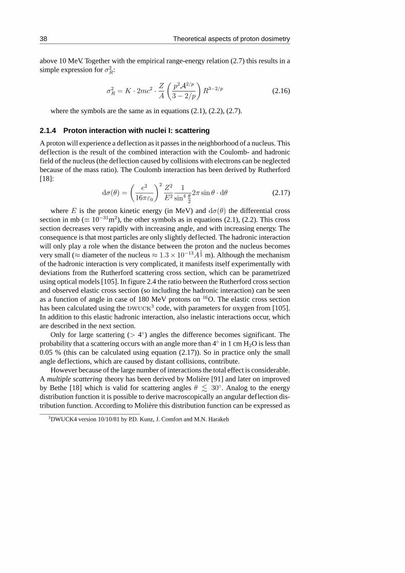
where. is the proton kinetic energy (in MeV) and_jEwä the differential crosssection in mb (ì 103ô�m2), the other symbols as in equations (2.1), (2.2). This crosssection decreases very rapidly with increasing angle, and with increasing energy. Theconsequence is that most particles are only slightly deflected. The hadronic interactionwill only play a role when the distance between the proton and the nucleus becomesvery small (ä diameter of the nucleusä �éôû �f3�ôø
�ô m). Although the mechanism
of the hadronic interaction is very complicated, it manifests itself experimentally withdeviations from the Rutherford scattering cross section, which can be parametrizedusing optical models [105]. In figure 2.4 the ratio between the Rutherford cross sectionand observed elastic cross section (so including the hadronic interaction) can be seenas a function of angle in case of 180 MeV protons on�SO. The elastic cross sectionhas been calculated using theaçýW"3 code, with parameters for oxygen from [105].In addition to this elastic hadronic interaction, also inelastic interactions occur, whichare described in the next section.
Only for large scattering (: 4á) angles the difference becomes significant. Theprobability that a scattering occurs with an angle more than 4á in 1 cm H2O is less than0.05 % (this can be calculated using equation (2.17)). So in practice only the smallangle deflections, which are caused by distant collisions, contribute.
However because of the large number of interactions the total effect is considerable.A multiple scatteringtheory has been derived by Molière [91] and later on improvedby Bethe [18] which is valid for scattering angles w í ôfá. Analog to the energydistribution function it is possible to derive macroscopically an angular deflection dis-tribution function. According to Molière this distribution function can be expressed as
3DWUCK4 version 10/10/81 by P.D. Kunz, J. Comfort and M.N. Harakeh

2.1 Proton interaction with matter 39
deflection angle (degrees)
diff
eren
tial c
ross
sec
tion
(mb/
sr)
ratio total/rutherford
0 10 20 30 40 50 60 70 80 90
10-3
10-2
10-1
100
101
102
103
0
2
4
6
8
10
12
14
16
Figure 2.4: Solid line (scale on right axis): ratio between total elastic cross section of 180 MeV protons
incident on49O (usingaçýW"g ) and Coulomb contribution (using equation (2.17) ) as a function of
deflection angle. Dotted line: ratio = 1. Dashed line (scale on left axis): Coulomb contribution.
a series expansion which involves complicated functions. The limiting case for manycollisions again is a Gaussian distribution:
sEwä_w '�s2Zw2f
i T
%ýëwT*@?i2wf
ê2&_w (2.18)
For the calculation of the widthwf (the mean squared scattering angle projected on aplanewh4t
T*@?i , which is �I2wh4ttT@Ui ) of the Gaussian several approximations exist. In [52]
is shown experimentally that the Highland formulagives the best results for protons:
wf ä �eé� �iV
q2E. n�S2ä
u|
u-
é� n
�
b*L}�f
ë|
u-
êèh@_ (2.19)
where| is the thickness of the medium,. the proton kinetic energy, �S2 the protonrest mass (expressed in MeV) andu- the radiation length of the material, which isthe distance over which the electron energy is reduced to a factor 1/e due to brems-strahlung only (this is tabulated e.g. in [77], for wateru- = 36.1g/cm2). Although theradiation length is a material property derived for electrons, this formula turns out tofit the experimental data with protons well [52]. For small angles we can approximatew2tT@Ui ä Ew2T*@?ic n w
2T*@?ic)ä. The deflection in% and+ - direction are independent and
identical distributed. The Highland formula works under the assumption that the pro-ton kinetic energy remains constant during the passage, which means that the thickness

40 Theoretical aspects of proton dosimetry
proton energy (MeV)
Inel
astic
cro
ss s
ectio
n ( mb )
0 50 100 150 200 2500
100
200
300
400
500
600
Figure 2.5: Total nonelastic nuclear cross section for protons incident on49O. The line represents a fit
using the}ABtû code [141] to the experimental data.
| has to be small. In the case of thick absorbers, it is possible to apply equation (2.19)to a thin slab and in analog way as for the energy straggling by taking the sum of thew2f of the individual slabs. Because of the artificial use of the radiation length however,
it is necessary to remove the factork� n �
b*L}�f
í|u-
ìlfrom the integral, thus treating
it as a correction factor which depends on theentire target thickness [52].The pathlength travelled by the proton will increase due to the multiple scattering
process. This means that the average penetration depth~ of the protons will be shorterthan theirWtaB range-. The difference between the lengths can be calculated using[18]:
E-ý ~ä '] .f
f
E�ý ULt wä
ëý_._5
ê3�_. (2.20)
whereE-ý ~ä is the mean difference andE�ý SJrEwää the mean deflection angle.In [67] they are tabulated for different materials: it turns out that for protons in waterthe effect is negligible above 1 MeV.
2.1.5 Proton interaction with nuclei II: nuclear reactions
Because the energy of the proton in radiotherapy applications is much higher than theCoulomb-barrier, protons will have a probability of reacting with the nucleus otherthan by elastic or inelastic scattering. This causes a decrease of the proton flux withdepth, already long before the end of the proton range. When we assume theWtaB

2.1 Proton interaction with matter 41
prot
on f
lux
per
inci
dent
pro
ton
depth (cm)0 5 10 15 20
0.0
0.2
0.4
0.6
0.8
1.0
80 MeV
180 MeV
Figure 2.6: Proton flux reduction due to inelastic nuclear reactions for a 80 and a 180 MeV beam in a
water medium calculated using equation (2.21) and the cross sections in figure 2.5.
approximation (see equation (2.6)), this can be described by:
x ' xf i T
ëý4ù@ñøig
] .f
.
jð?i*@tE.âä
_.â
7E.âä
ê(2.21)
wherex is the flux of protons with energy ., xf the initial flux,.f the start energy,7E.ä the stopping power andjð?i*@tE.ä the inelastic nuclear reaction cross section.For radiotherapy applications (where water is the reference material) we are mainlyinterested in the cross section with oxygen because the reaction cross section withhydrogen is negligible [71]. The�SO cross section has been measured by Carlsson etal. [28] and by Renberg et al. [109]. Figure 2.5 shows the experimental points togetherwith a fit that has been made by Seltzer [16] using the}ABtû-code [141].
With respect to the reaction products the situation is more complicated. The sec-ondary particles can be neutrons, protons and recoil fragments. The energy transferredto the recoil fragments will be deposited locally, but secondary protons can travel aconsiderable distance before stopping. The secondary neutrons will either escape fromthe medium or produce another nuclear reaction, in which tertiary particles can be pro-duced. Ingeneral it is not possible to make an analytical calculation of the contributionof nuclear reactions to the energy deposition as a function of depth. Berger [16] usesthe estimate that 60 % of the initial proton energy (i.e. before the reaction) is depositedlocally while the other 40 % escapes from the medium in the form of neutrons andò’s.Monte Carlo calculations, however, in which the secondary particles are separately fol-lowed are not in agreement with this and show that a depth dependent contribution is

42 Theoretical aspects of proton dosimetry
deposited (see section 3.4). The result for the flux reduction of the primary protons us-ingequation (2.21) can be seen in figure 2.6. The steepness of flux reduction is slightlylarger for the 80 MeV proton beam, due the slightly higher cross section.
2.1.6 Proton dose distributions
When we summarize the results of the previous sections, it is possible to calculate theproton dose (=energy lost to the medium) as a function of position. We start with thedose dependence in the direction parallel to the beam. We define the energy fluence[at depth5 by:
[E5ä ' xE5ä.E5ä (2.22)
wherex is the proton flux, and. the proton kinetic energy as a function of depth5.The energy loss by the protons as a function of depth is thengiven by:
(E5ä ' ý�4
_[E5ä
_5' ý�
4
ëxE5ä
_.E5ä
_5n F_xE5ä
_5.E5ä
ê(2.23)
The first term describes the energy lost to the atomic electrons (see sections 2.1.2,2.1.3). In first approximation we assume that this energy is deposited locally (this ap-plies when the medium is water, for air this is not the case, see section 2.2). The sec-ond term describes the energy lost by the flux reduction due to nuclear interactions.Here the assumption of local deposition is no longer valid. The best thing we can doanalytically is to use the approximation that a fractionF of 0.6 is deposited locally,while the remaining energy escapes in the form of neutrons andò’s (see however sec-tions 2.1.5, 3.4). Using these assumptions, the energy loss(E5ä in equation (2.23) isequal to the deposited dose.
Using the empirical relation between. and- given in relation (2.7), it’s possibleto simplify the calculation considerably.
The energy .E5ä at a depth5 is determined by the residual range-fý 5 which theprotons traverse before stopping:
.E5ä '�
D�*R E-f ý 5ä�*R (2.24)
From this we can determine d./d5:
_.
_5'ý�RD�*R
ý-f ý 5ä�*R3�
ü(2.25)
With respect to the flux reduction due to nuclear reactions, we can use equation (2.21),but in [76] it is shown that the error resulting from ignoring the energy dependence ofthe cross sectionjð?i*@t and using a straight line fit:
xE5ä ' xf� n EE-f ý 5ä
� n E-f (2.26)

2.1 Proton interaction with matter 43
is small compared to the uncertainty on the position of energy deposition of the sec-ondary particles (see also figure 2.6). Therefore:
_x
_5' ýxf E
E� n E-fä (2.27)
whereE is a medium dependent parameter andxf the initial flux.In order to incorporate the range straggling caused by the energy straggling in the
medium and the initial energy spread of the proton beam, the relevant distributionfunctions have to be folded into equation (2.23). Bortfeld has shown [23] that it ispossible to do so, with a limited number of simplifications to the proton energy spectra:for the range straggling he uses the Bohr approximation (2.16) and for the initial beamspread the sum of a Gaussian and a small ‘tail’ extended towards low energies. Theresult is a rather complicated expression:
(E5ä ' xfe3l
2*ej�*RKE�*Räs2Z4RD�*RE� n E-fä
ûé�
jG3�*REýlä n
ëERn F n 0
-f
êG3�*R3�Eýlä
è(2.28)
whereG is the parabolic cylinder function,K is thegamma function (both tabulated in[3]) andl isE-fý5ä*jwherej is the total width of the range straggling. The parameter0 describes the low energy tail of the initial proton spectrum. This tail contains a smallfraction of the initial flux, but is influenced by the way a proton beam is produced.In the calculations0 has been set to zero. The total width consists of a termj24L?L
caused by the energy straggling in the medium and a termj2.f caused by the initialbeam spread. The totalj can be calculated with:
j2 ' j24L?L n j2.f
ë_-f_.f
ê2' j24L?L n j
2.fD2R2.E2R32äf (2.29)
j4L?L is the range straggling that is present for a monoenergetic beam and can be calcu-lating using equation (2.16). The other, medium dependent parameters are determinedby equations (2.7), (2.23), (2.27). A summary of the parameters isgiven in table 2.3together with the values in case the medium is water.
Although expression (2.28) looks complex, it is easy to evaluate numerically. Infigure 2.7 we see dependence of the height of theBragg peakas a function of initialenergy spreadj.f both for a 80 and a 175 MeV proton beam. Also the position of theBragg peak changes. The definition for the term ‘Bragg peak’ subsequently used inthis thesis is the position where themaximaldose occurs. In figure 2.7 and subsequentfigures we plot the dose per flux instead of the dose, which means that to obtain a dosethis value has to be multiplied with the number of protons per cm2.
The range-f for 180 MeV protons is 21.64 cm. It can be seen in figure 2.7 thatthis equals the depth at which the dose has dropped to 80÷ 1 % of its maximum value

44 Theoretical aspects of proton dosimetry
Table 2.3:The parameters which determine equation (2.28) together with their numerical values in case
of a water medium. The last two parameters are beam dependent
description value for water unit
s exponent of range-energy relation 1.74 1
D proportionality factor of ’’’’ 2.56ü103ô cm MeVýs
U3 range DHs3 cm
E slopeparameter of flux reduction 0.012 cmý4
F fraction of energy released locally 0.6 1
â4L?L width of range straggling 0.012U3=<683 cm
âH3 initial beam width$ beam dependent ä 0.01H3 MeV
% contribution to tail$ beam dependent ä 0.0-0.2 1
beyond the Bragg peak,independentof the initial energy spread. This is known as the5Hf ' -f empirical rule of thumb [16].
With respect to the dose distribution in the lateral direction we can make use ofthe Gaussian approximation of the multiple scattering theory as is described in sec-tion 2.1.4. The total width of the proton beam isgiven by the quadratic sum of thewidth caused by the initial divergence of the proton beam and the (depth dependent)broadeningcaused by multiple scattering. The result for a parallel beam (with no initialdivergence) can be seen in figure 2.8. The multiple scattering increases in the Braggpeak, due to the�*. dependence of the scattering angle. Fortwo or more dimensionalproblemsit is in general not possible to use analytical tools. To calculate the distribu-tion in figure 2.8 we have therefore used a numerical method: the Monte Carlo codeV|iBA [16]. In chapter 3 we present more details on the this code, together with com-parisons between experimental data, equation (2.28) and other Monte Carlo codes.

2.1 Proton interaction with matter 45
R0 = 21.64 cm
dose
per
flu
ence
(M
eV c
m
2
/g)
depth (cm)19 20 21 22 23
0
5
10
15
20
25
30
dose
per
flu
ence
(M
eV c
m
2
/g)
depth (cm)
180 MeV
2 3 4 5 60
10
20
30
40
50
60
R0 = 5.19 cm
80 MeV 0 %
1.5 % 1.5 %
0 %
Figure 2.7: The dose per fluence as a function of depth in water calculated with (2.28) for 80 and
180 MeV proton beams, with an initial energy spreadâ increasing from 0 % to 1.5 % in steps of
0.25%. Entrance dose per fluence is for a 180 MeV beam 5.78 MeV cm5 /g and for a 80 MeV beam
9.32 MeV cm5 /g. R3 is shown as the dashed line.
14.5 15 15.5 16 16.5 17 17.5 180
0.5
1
1.5
2
2.51%
10%
20%
30%
40%50%
60%70%
80%90%
99%
depth(cm)
radi
al d
ista
nce
(cm
)
Figure 2.8: Contour plot of dose of a 160 MeV, 2 cm radius parallel proton beam in water. The contour
lines go from 1% to 99% of the maximum dose. Calculated withV|iBA [16]. At zero depth and on the
beam axis the dose is 21% of the dose in the Bragg peak.

46 Theoretical aspects of proton dosimetry
2.2 Proton dose measurement
2.2.1 Introduction
A measurement of the absorbed dose distribution necessitates the introduction of aradiation-sensitive device into the medium. Normally, this device will differ from themedium in both atomic number and density and it therefore constitutes a discontinuity,which will be referred to as acavity, see figure 2.9.
In this section we will examine the influence of the detector properties on the resultof the dose measurements. We start with the most simple situation where the detectorhas the same material properties as the medium, we extend this to other material prop-erties (Bragg-Gray theory) and to non-local energy deposition (Spencer-Attix theory).Finally we examine the relation between the energy absorbed in the medium and thedosimeter signal in case the dosimeter is an ionization chamber. The case where thedosimeter is a scintillator will be discussed in sections 3.5.4, 4.1.2.
2.2.2 Influence of detector geometry
In case the detector material is equal to the medium material, we can assume that theinfluence of boundaries can be neglected. Since the detector is thin, we neglect thechange in proton flux caused by nuclear interactions. The stopping power7E.ä isenergy dependent, therefore we have to integrate over the complete energy spectrum.The dose at a detector position5 is thengiven by:
(U@ñE5ä '�
4
] .f
f
xE.c 5ä ü 7E.ä ü _. (2.30)
where is(E5ä the dose,xE.c 5ä the proton flux at position5 and7E.ä the pro-ton stopping power. In first approximation we assume that the fluxxE.c 5ä does notchange under influence of the detector and that the energy lost by the proton is de-posited locally. In reality the detector is not infinitesimal thin, which means that the
beam
medium
z t
cavity
Figure 2.9: A schematic overview of a cavity in a medium which has the purpose of measuring dose
distributions.

2.2 Proton dose measurement 47
t = 5 mm
t = 1 mm
t = 0.1 mm 180 MeV
depth (cm)do
se p
er f
luen
ce (
MeV
cm
2 /g
)
20 21 220
5
10
15
20
25
30
depth (cm)
80 MeV
dose
per
flu
ence
(M
eV c
m
2
/g)
4 5 60
10
20
30
40
50
60
t = 5 mm
t = 1 mm t = 0.1 mm
Figure 2.10: Influence of detector thickness for a water equivalent detector on the measurement of the
Bragg peak in water for a monoenergetic 80 and 180 MeV proton beam. Infinitesimal thin andw = 0.1
mm detector thicknesses are almost indistinguishable both for 80 and 180 MeV. The dose distribution
for an infinitesimal thin detector has been calculated using the analytical model (2.28).
stopping power7E.ä ì _._5
has to replaced by {*| where{ is the mean energy lossin the detector with thickness|:
(U@ñE5ä '�
4
] .f
f
xE.c 5ä{
|_. (2.31)
This averaging can cause major distortions in the observed Bragg peak, especiallyfor low energy (é 80 MeV, mainly used for ocular melanoma) beams were the detector4ü| is not small anymore compared to the width of the Braggpeak. The observed Braggpeak will be shifted to the left and broadened compared to the actual dose distributiongiven by equation (2.30). This is illustrated in figure 2.10 for a 80 and a 180 MeVproton beam (calculated using the analytical model (2.28)). It is clear that the smallerthe cavity size the less distortions in the measured dose distribution occur.
2.2.3 Bragg-Gray theory
The main interest, however, is not the dose in the cavity, but rather the dose in themedium as it would be in absence of the detector. Therefore one has to account fordifferences in material property between the medium and detector material. In firstapproximation we can multiply equation (2.31) with the spectrum averaged protonstopping power ratios [18]:
(4i_E5ä ' (U@ñE5ä4U@ñ44i_
U .ff74i_E.äxE.c 5ä_.U .f
f7U@ñE.äxE.c 5ä_.
(2.32)

48 Theoretical aspects of proton dosimetry
This relation is known as the Bragg-Gray relation, and was originally derived forX-rays by Gray [53]. X-rays areindirectly ionizing, which means that the energy isdeposited by the electrons produced by the photo-electric effect, Compton scatteringor pair-creation. These electrons are calledprimary electrons. Therefore in the Bragg-Gray relation for X-rays the stopping power ratio for the primary electrons has to beused. The fundamental assumptions of the Bragg-Gray cavity theory are:
1. the cavity is so small that the fluxxE.c %ä is unchanged.
2. the energy lost is deposited locally.
3. the energy loss is continuously. For this anelectron equilibriumis necessary,which means that the same number of electrons will enter and exit the cavity(from the medium or by backscattering).
Assumption 2 clearly is not valid when energetic, B electrons are produced in asmall cavity. For X-rays the Bragg-Gray equation (2.32) has been extended by Spencerand Attix, which is described in the next section. For protons the situation is less clear.Although protons do have direct (local) energy loss, they can also produce energeticB-electrons which are not absorbed locally (see section 2.1.3). We have made studiesof this effect using Monte Carlo methods together with experimental data. This will bepresented in section 3.5.
The Bragg-Gray relation (2.32) alone shows already a large influence of the cavitymaterial on the shape of the observed Bragg peak. Because the mean excitation poten-tial is present in the logarithmic term of equation (2.4), the ratio of stopping powers isenergy dependent (see table 2.1). The result for 80 and 180 MeV proton beams whenthe detector material is air, silicium, carbon orgadolinium can be seen in figure 2.11(using proton flux spectraxE.c 5ä that have been calculated with theV|iBA code, seesection 3.2).
It can be seen that the difference in distortion between a 80 and a 180 MeV beamis smaller than the difference in distortion caused by the finite detector size (cf. fig-ure 2.10). It can also be seen that the error made by neglecting differences in materialin case of air or carbon detectors is very small, 1 %.
2.2.4 Spencer-Attix theory
For X-rays deviations between equation (2.32) and experimental data (for exampleusing water calorimetry, see next section) have been found. Spencer and Attix havederived a theory which accounts for these deviations by taking the creation of sec-ondary B-electrons into account [121]. For X-rays this secondary electrons are createdby the primary electrons (which themselves have an energy comparable to the incidentX-rays). The creation of secondary electrons in case the primary particle is a protonhas been treated in section 2.1.3. In the Spencer-Attix theory, the secondary electrons

2.2 Proton dose measurement 49
depth (cm)
dose
per
flu
ence
(M
eV c
m
2
/g)
dose
per
flu
ence
(M
eV c
m
2
/g)
gadolinium
silicium
2 3 4 5 60
10
20
30
40
50
60
gadolinium
silicium80 MeV
depth (cm)
180 MeV
19 20 21 22 230
5
10
15
20
25
30
Figure 2.11: Depth-dose curves for different detector materials. Solid lines represent curves for water,
air and carbon which are indistinghuishable both for 80 and 180 MeV. Dash-dotted line: gadolinium
and dashed line: silicium. The entrance dose of the air,carbon,silicium and gadolinium is normalized to
the entrance dose of water.
are separated into twogroups, divided at a cut-off energy { that corresponds approx-imately to the energy of an electron that canjust cross the cavity. A typical airgap inan ionization chamber is in the order of 2 mm* 0.24 mg/cm2, which is slightly belowthe range of 10 keV electrons. A typical choice of{ is therefore 10 keV. A ‘slow’secondary electron, with an energy less than{, is considered to dissipate its energyat the point at which it isgenerated. The ‘fast’ secondary electrons (theB-electrons insection 2.1.3), with an energy greater than{, are also considered as primary particlesthat have a continuous energy loss, and their energy is not considered to have beendissipated until they have dropped below{. Since the fast secondary electrons areaccounted for separately, their energy should not be included in the primary stoppingpower, which is now restricted to energy losses less than{. It is assumed that slowelectrons released into the cavity from the chamber wall are in equilibrium with otherslow electrons released from thegas that impinge upon the chamber wall, so that thereis no net energy transfer. The energy interval just above{ deserves special attention,because for that interval the particles can originate from outside the cavity, but stopinside. This contribution is called thetrack-end termA, [2,9,65,84]. When we applythis to protons, relation (2.32) has to be split into a proton and aB-electron term:
(4i_E5ä ' (U@ñE5ä ü%4U@ñ44i_
üU .f{ýR4i_E.äxRE.c 5ä_. n A, R4i_E5ä n ü ü üU .f
{ýRU@ñE.äxRE.c 5ä_. n A, RU@ñE5ä n ü ü ü
ü ü ün U A4@
{7B4i_E.äxBE.c 5ä_. n A, B4i_E5ä
ü ü ün U A4@
{7BU@ñE.äxBE.c 5ä_. n A, BU@ñE5ä
&(2.33)
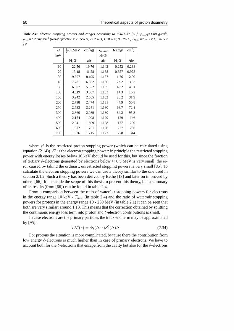
50 Theoretical aspects of proton dosimetry
Table 2.4: Electron stopping powers and ranges according to ICRU 37 [66].ãK5R=1.00 g/cm6,
ãdlu=1.20 mg/cm6 (weight fractions: 75.5% N, 23.2% O, 1.28% Ar, 0.01% C)LK5R=75.0 eV, Ldlu=85.7
eV
. 447 (MeV cm5/g) rçc@ðo - (mg/ cm5)
keV H5O/
H5O air air H5O Air
10 22.56 19.76 1.142 0.252 0.288
20 13.18 11.58 1.138 0.857 0.978
30 9.657 8.495 1.137 1.76 2.00
40 7.781 6.852 1.136 2.92 3.32
50 6.607 5.822 1.135 4.32 4.91
100 4.119 3.637 1.133 14.3 16.2
150 3.242 2.865 1.132 28.2 31.9
200 2.798 2.474 1.131 44.9 50.8
250 2.533 2.241 1.130 63.7 72.1
300 2.360 2.089 1.130 84.2 95.3
400 2.154 1.908 1.129 129 146
500 2.041 1.809 1.128 177 200
600 1.972 1.751 1.126 227 256
700 1.926 1.715 1.123 278 314
whereýR is the restricted proton stopping power (which can be calculated usingequation (2.14)).7B is the electron stopping power: in principle the restricted stoppingpower with energy losses below 10 keV should be used for this, but since the fractionof tertiary B-electronsgenerated by electrons belowä 0.5 MeV is very small, the er-ror caused by taking the ordinary, unrestricted stopping powers is very small [85]. Tocalculate the electron stopping powers we can use a theory similar to the one used insection 2.1.2. Such a theory has been derived by Bethe [18] and later on improved byothers [66]. It is outside the scope of this thesis to present this theory, but a summaryof its results (from [66]) can be found in table 2.4.
From a comparison between the ratio of water/air stopping powers for electronsin the energy range 10 keV -A4@ (in table 2.4) and the ratio of water/air stoppingpowers for protons in the energy range 10 - 250 MeV (in table 2.1) it can be seen thatboth are very similar: around 1.13. This means that the correction obtained by splittingthe continuous energy loss term into proton andB-electron contributions is small.
In case electrons are the primary particles the track end term may be approximatedby [95]:
A, BE5ä ' xBE{c 5ä7BE{ä{ (2.34)
For protons the situation is more complicated, because there the contribution fromlow energy B-electrons is much higher than in case of primary electrons. We have toaccount both for theB-electrons that escape from the cavity but also for theB-electrons

2.2 Proton dose measurement 51
that enter through the chamber wall (from the medium or backscattered). In [75] asimplified calculation for agas chamber with thin walls is presented, resulting in anet loss of 2.3 % of the total energy deposited in the cavity due toB-electron escape.When the thickness of the walls is increased (as is the situation for a chamber in amedium) this loss decreases to 0.8 %. In addition to this effect, where the wall materialwas assumed to be equal to the medium material, differences occur when the wallconsists of a different material (for example carbon, or PMMA). This also effects thetrack end terms. Although some preliminary studies have been performed [85, 101],it remains unclear how to calculate these wall correction factors for protons. In theBBV64 dosimetry protocol from 1986 [1] theB-electrons have been pointed out to be amajor difficulty and in 10years the situation has not become clearer. Also Monte Carlocalculations are very difficult because of the small energies and distances involved. Insection 3.5 we present some results obtained with}jBA|.
2.2.5 Ionometry
For the actual measurement of the dose that is deposited in the cavity, one can ex-ploit the experimental fact that the average energy that is needed to create an ion pairis nearly independent of the proton energy. It is also nearly the same fork-particles,protons and electrons. Moreover, the energy is not very different for different stop-ping gases and, contrary to naive expectation, is smallest for the inertgases whoseionization potentials are the highest of all atoms. These facts have been explained ina semi-quantitative theory by Fano [18, 39]. Instead of the energy of just the proton,Fano considers the total energy available for ionization, whether it resides in the pro-ton or in aB-electron. In a collision in which the atom is excited (cross sectionje) byeither a proton or aB-electron, the available energy is reduced by the excitation energy`e. If the atom is ionized and the kinetic energy of the ejected electron is less thanthe ionization potentialUðL? (cross sectionjUðL?� ), the total energy given to the atomicelectron`UðL?� is lost from the available energy. However, if an electron of kineticenergy greater thanUðL? is produced (cross sectionjUðL?2 ), its kinetic energy is avail-able for further ionization, and the loss of available energy is considered to be onlythe ionization potentialUðL? . The average amount of (available) energy spent per ion isthen:
ç 'je`e n jUðL?�`UðL?� n jUðL?2 UðL?
jUðL?� n jUðL?2(2.35)
Now the ratio of the various cross sections, especially of je andjUðL?� , does not changemuch with the proton energy. This does also hold for the average energies`e and`UðL?� . SincejUðL?2 á jUðL?� , this explains in a qualitative way the independence ofçfrom proton energy.
The independency of ç with proton energy does not hold exactly, especially forgases such as air which have a low ionization potentialUðL? (nitrogen: 15.5 eV, oxygen:
4American Association of Physicists in Medicine

52 Theoretical aspects of proton dosimetry
12.5 eV) and much energy is ‘wasted’ to excitations. For clinical purposes however theuse of air is desirable, to avoid complicatedgas systems. The usual way of determin-ing theç value is by comparing a water calorimeter result with an air-filled ionizationchamber result [118]. Through theyears a large number of measurements of thisçvalue has been performed, which however do not completely agree with each other. Aproblem is that the experimental value obtained is the productrçc@ðh ü ç. This meansthat the result also depends on the stopping power values one is using. Another com-plication is that the humidity of air influencesç in a different way thanrçc@ðh . Analogto the stopping power calculations it has been tried to achieve uniformity through rec-ommendations: unfortunately forç there remain two competing values: 34.3 eV in [1]and 35.2 eV in [64,135,136]. Until more accurate measurements are available this willbe a major source of systematic uncertainty in absoluteproton dosimetry.
2.2.6 Ion recombination correction
Not all the ions that are created in an ionization chamber will be collected by the elec-trodes. Some of the ions will meet electrons before they can reach the electrodes. Thisrecombinationcan be reduced by sweeping the ions out of the chamber more rapidly,either by increasing the field strength or by reducing the distance between the elec-trodes. In [21] a theoretical description for this recombination isgiven, in which acollection efficiency s for a parallel plate ionization chamber is derived:
s '�ý
� n6 ü ^ ü _eL2
ü (2.36)
where^ is the ionization rate (in C cm3ô s3�), _ the distance between the electrodes(in mm, for a Markus orABWV chamber 2 mm) andL the chamber voltage (in V).6is a constant, characteristic of thegas at agiven temperature and pressure. For air atSTP conditions its value is:6 = 6.73ü10�� C3� V2 s cm3�. This can be converted to acorrection factor&r which depends on the doserateù( (Gy/s):
&r ' � n6( ü ù( ü _e
L2(2.37)
where the actual dose is&r times the measured dose,6( = 2.4 Gy3� s V2 cm3e
for air at STP condition. In the spot scan technique (see section 5.2.1) the most distalspots are ingeneral reached only once. This means that the complete dose (in the orderof ä 1-2 Gy) has to be delivered in 10 ms. It can be seen that even in this case thecorrection is minimal, because high voltages up to 3 kV/cm can be used.


