THEORETICAL AND PRACTICAL ASPECTS ON THE …webee.technion.ac.il/people/sason/Gil_PhD_thesis.pdf ·...
265
THEORETICAL AND PRACTICAL ASPECTS ON THE PERFORMANCE VERSUS COMPLEXITY TRADEOFF FOR LDPC-BASED CODES GIL WIECHMAN
Transcript of THEORETICAL AND PRACTICAL ASPECTS ON THE …webee.technion.ac.il/people/sason/Gil_PhD_thesis.pdf ·...

THEORETICAL AND PRACTICAL
ASPECTS ON THE PERFORMANCE
VERSUS COMPLEXITY TRADEOFF
FOR LDPC-BASED CODES
GIL WIECHMAN

THEORETICAL AND PRACTICAL ASPECTS
ON THE PERFORMANCE VERSUS
COMPLEXITY TRADEOFF FOR LDPC-BASED
CODES
RESEARCH THESIS
SUBMITTED IN PARTIAL FULFILLMENT OF THE
REQUIREMENTS
FOR THE DEGREE OF DOCTOR OF PHILOSOPHY
GIL WIECHMAN
SUBMITTED TO THE SENATE OF THE TECHNION — ISRAEL INSTITUTE OF TECHNOLOGY
Shebat 5768 HAIFA JANUARY 2008

THIS RESEARCH THESIS WAS SUPERVISED BY DR. IGAL SASON UNDER
THE AUSPICES OF THE DEPARTMENT OF ELECTRICAL ENGINEERING
ACKNOWLEDGMENT
I wish to thank my supervisor, Dr. Igal Sason, for his dedicated guidance and for
contributing greatly to the research and the analysis presented in this dissertation.
The enjoyment and delight-in-doing which I have experienced during my time at the
Technion is largely due to him. It has been a great privilege to work in a fruitful
and enjoyable cooperation with a researcher of his caliber. I wish to thank him for
instilling in me some of his curiosity and his strong desire to fully understand any
problem we chose to tackle. Moreover, his warm and friendly attitude, patience, and
true willingness to help and contribute in any professional and personal hardship will
remain with me for years to come.
I also wish to thank my parents, Rivka and Menachem, for their encouragement and
support. Ever since I can remember, education and scholarship have always been a
first priority in my family. This work is undoubtedly a direct result of these values.
This work could not have been accomplished without the warm support of my wife,
Anat. My heartfelt gratitude goes to her for her encouragement, support, and under-
standing during the numerous evening and nights when my mind had drifted away
from the daily affairs of our home. She has been a perfect companion in the long and
challenging journey which we traveled in the last few years.
The generous financial help of Andrew and Erna Finci Viterbi, the Ne’eman
Foundation, and the Technion is gratefully acknowledged.
This research was supported by the Israel Science Foundation (grant no. 1070/07).


Contents
Abstract 1
Notation 3
Abbreviations 4
1 Introduction 6
1.1 Linear Block Codes . . . . . . . . . . . . . . . . . . . . . . . . . . . . 6
1.2 Gallager’s LDPC Codes . . . . . . . . . . . . . . . . . . . . . . . . . 7
1.3 The Re-Discovery of Graph-Based Codes . . . . . . . . . . . . . . . . 8
1.4 Motivation and Related Work . . . . . . . . . . . . . . . . . . . . . . 11
1.5 This Dissertation . . . . . . . . . . . . . . . . . . . . . . . . . . . . . 14
2 Parity-Check Density versus Performance of Binary Linear Block
Codes over Memoryless Symmetric Channels: New Bounds and Ap-
plications 18
2.1 Introduction . . . . . . . . . . . . . . . . . . . . . . . . . . . . . . . . 19
2.2 Preliminaries . . . . . . . . . . . . . . . . . . . . . . . . . . . . . . . 23
2.3 Approach I: Bounds Based on Quantization of the LLR . . . . . . . . 26
2.3.1 Bounds for Four-Levels of Quantization . . . . . . . . . . . . . 27
2.3.2 Extension of the Bounds to 2d Quantization Levels . . . . . . 37
2.4 Approach II: Bounds without Quantization of the LLR . . . . . . . . 46
2.5 Numerical Results . . . . . . . . . . . . . . . . . . . . . . . . . . . . . 58
d

CONTENTS e
2.5.1 Thresholds of LDPC Ensembles under ML Decoding . . . . . 59
2.5.2 Lower Bounds on the Bit Error Probability of LDPC Codes . 63
2.5.3 Lower Bounds on the Asymptotic Parity-Check Density . . . . 64
2.6 Summary and Outlook . . . . . . . . . . . . . . . . . . . . . . . . . . 66
2.A Some mathematical details related to the proofs of the statements in
Section 2.3.1 . . . . . . . . . . . . . . . . . . . . . . . . . . . . . . . . 70
2.A.1 Proof of Lemma 2.2 . . . . . . . . . . . . . . . . . . . . . . . . 70
2.A.2 Derivation of the Optimization Equation in (2.24) and Proving
the Existence of its Solution . . . . . . . . . . . . . . . . . . . 70
2.A.3 Proof of Inequality (2.33) . . . . . . . . . . . . . . . . . . . . 73
2.B Some mathematic details for the proof of Proposition 2.3 . . . . . . . 74
2.B.1 Power Series Expansion of the Binary Entropy Function . . . 74
2.B.2 Calculation of the Multi-Dimensional Integral in (2.65) . . . . 75
2.C Some mathematical details related to the proofs of the statements in
Section 2.4 . . . . . . . . . . . . . . . . . . . . . . . . . . . . . . . . . 76
2.C.1 On the Improved Tightness of the Lower Bound in Theorem 2.5 76
2.C.2 Proof for the Claim in Remark 2.5 . . . . . . . . . . . . . . . 78
2.C.3 Proof of Eq. (2.82) . . . . . . . . . . . . . . . . . . . . . . . . 79
2.C.4 Proof of Eq. (2.83) . . . . . . . . . . . . . . . . . . . . . . . . 80
3 On Achievable Rates and Complexity of LDPC Codes over Parallel
Channels: Bounds and Applications 82
3.1 Introduction . . . . . . . . . . . . . . . . . . . . . . . . . . . . . . . . 83
3.2 Bounds on the Conditional Entropy for Parallel Channels . . . . . . . 85
3.2.1 Lower Bound on the Conditional Entropy . . . . . . . . . . . 85
3.2.2 Upper Bound on the Conditional Entropy . . . . . . . . . . . 91
3.3 An Upper Bound on the Achievable Rates of LDPC codes over Parallel
Channels . . . . . . . . . . . . . . . . . . . . . . . . . . . . . . . . . . 92
CONTENTS f
3.4 Achievable Rates of Punctured LDPC Codes . . . . . . . . . . . . . . 99
3.4.1 Some Preparatory Lemmas . . . . . . . . . . . . . . . . . . . . 100
3.4.2 Randomly Punctured LDPC Codes . . . . . . . . . . . . . . . 102
3.4.3 Intentionally Punctured LDPC Codes . . . . . . . . . . . . . . 106
3.4.4 Numerical Results for Intentionally Punctured LDPC Codes . 108
3.5 Lower Bounds on the Decoding Complexity of LDPC Codes for Parallel
Channels . . . . . . . . . . . . . . . . . . . . . . . . . . . . . . . . . . 113
3.5.1 A Lower Bound on the Decoding Complexity for Parallel MBIOS
Channels . . . . . . . . . . . . . . . . . . . . . . . . . . . . . . 113
3.5.2 Lower Bounds on the Decoding Complexity for Punctured LDPC
Codes . . . . . . . . . . . . . . . . . . . . . . . . . . . . . . . 117
3.5.3 Re-Derivation of Reported Lower Bounds on the Decoding Com-
plexity . . . . . . . . . . . . . . . . . . . . . . . . . . . . . . . 120
3.6 Summary and Outlook . . . . . . . . . . . . . . . . . . . . . . . . . . 120
3.1 Re-derivation of [65, Theorems 3 and 4] . . . . . . . . . . . . . . . . . 122
4 Bounds on the Number of Iterations for Turbo-Like Ensembles over
the Binary Erasure Channel 125
4.1 Introduction . . . . . . . . . . . . . . . . . . . . . . . . . . . . . . . . 126
4.2 Preliminaries . . . . . . . . . . . . . . . . . . . . . . . . . . . . . . . 129
4.2.1 Graphical Complexity of Codes Defined on Graphs . . . . . . 129
4.2.2 Accumulate-Repeat-Accumulate Codes . . . . . . . . . . . . . 130
4.2.3 Big-O notation . . . . . . . . . . . . . . . . . . . . . . . . . . 133
4.3 Main Results . . . . . . . . . . . . . . . . . . . . . . . . . . . . . . . 133
4.4 Derivation of the Bounds on the Number of Iterations . . . . . . . . . 138
4.4.1 Proof of Theorem 4.1 . . . . . . . . . . . . . . . . . . . . . . . 138
4.4.2 Proof of Theorem 4.2 . . . . . . . . . . . . . . . . . . . . . . . 143
4.5 Summary and Conclusions . . . . . . . . . . . . . . . . . . . . . . . . 151

CONTENTS g
4.A Proof of Proposition 4.1 . . . . . . . . . . . . . . . . . . . . . . . . . 153
4.B Some mathematical details related to the proof of Theorem 4.2 . . . . 158
4.B.1 Proof of Lemma 4.2 . . . . . . . . . . . . . . . . . . . . . . . . 158
4.B.2 Proof of Lemma 4.3 . . . . . . . . . . . . . . . . . . . . . . . . 160
5 An Improved Sphere-Packing Bound for Finite-Length Codes over
Symmetric Memoryless Channels 161
5.1 Introduction . . . . . . . . . . . . . . . . . . . . . . . . . . . . . . . . 162
5.2 The 1967 Sphere-Packing Bound and Improvements . . . . . . . . . . 163
5.2.1 The 1967 Sphere-Packing Bound . . . . . . . . . . . . . . . . 164
5.2.2 Recent Improvements on the 1967 Sphere-Packing Bound . . . 170
5.3 An Improved Sphere-Packing Bound for Symmetric Memoryless Chan-
nels . . . . . . . . . . . . . . . . . . . . . . . . . . . . . . . . . . . . . 172
5.3.1 Symmetric Memoryless Channels . . . . . . . . . . . . . . . . 173
5.3.2 Derivation of an Improved Sphere-Packing Bound for Symmet-
ric Memoryless Channels . . . . . . . . . . . . . . . . . . . . . 175
5.4 The 1959 Sphere-Packing Bound of Shannon and Improved Algorithms
for Its Calculation . . . . . . . . . . . . . . . . . . . . . . . . . . . . . 185
5.4.1 The 1959 Sphere-Packing Bound and Asymptotic Approximations185
5.4.2 A Recent Algorithm for Calculating the 1959 Sphere-Packing
Bound . . . . . . . . . . . . . . . . . . . . . . . . . . . . . . . 189
5.4.3 A Log-Domain Approach for Computing the 1959 Sphere-Packing
Bound . . . . . . . . . . . . . . . . . . . . . . . . . . . . . . . 190
5.5 Numerical Results for Sphere-Packing Bounds . . . . . . . . . . . . . 191
5.5.1 Performance Bounds for M-ary PSK Block Coded Modulation
over Fully Interleaved Fading Channels . . . . . . . . . . . . . 192
5.5.2 Performance Bounds for M-ary PSK Block Coded Modulation
over the AWGN Channel . . . . . . . . . . . . . . . . . . . . . 194

CONTENTS h
5.5.3 Performance Bounds for the Binary Erasure Channel . . . . . 204
5.5.4 Minimal Block Length as a Function of Performance . . . . . 205
5.6 Summary . . . . . . . . . . . . . . . . . . . . . . . . . . . . . . . . . 210
5.A Proof of Lemma 5.1 . . . . . . . . . . . . . . . . . . . . . . . . . . . . 211
5.B Calculation of the Function µ0 in (5.47) for some Symmetric Channels 217
5.B.1 M-ary PSK Modulated Signal over Fully Interleaved Fading
Channels with Perfect CSI . . . . . . . . . . . . . . . . . . . . 217
5.B.2 M-ary PSK Modulated Signals over the AWGN Channel . . . 220
5.B.3 The Binary Erasure Channel . . . . . . . . . . . . . . . . . . . 220
5.C Proof of Proposition 5.3 . . . . . . . . . . . . . . . . . . . . . . . . . 222
6 Summary and Outlook 225
6.1 Contributions of this Dissertation . . . . . . . . . . . . . . . . . . . . 225
6.2 Future Research Directions . . . . . . . . . . . . . . . . . . . . . . . . 229
References 231
Hebrew Abstract

List of Figures
2.1 Channel model with four levels of quantization . . . . . . . . . . . . . 28
2.2 Comparison between lower bounds on the Eb
N0–thresholds under ML
decoding for right-regular LDPC ensembles. . . . . . . . . . . . . . . 62
2.3 Lower bounds on the bit error probability for any binary linear block
code transmitted over a binary-input AWGN channel whose capacity
is 12
bits per channel use. . . . . . . . . . . . . . . . . . . . . . . . . . 63
2.4 Comparison between lower bounds on the asymptotic parity-check den-
sity of binary linear block codes where the transmission takes place over
a binary-input AWGN channel. . . . . . . . . . . . . . . . . . . . . . 65
2.5 Plot of the binary entropy function to base 2 and some upper bounds
which are obtained by truncating its power series around x = 12. . . . 76
3.1 An interconnections diagram among the bounds in this paper and some
previously reported bounds which follow as special cases. . . . . . . . 121
4.1 Tanner graph of an irregular and systematic accumulate-repeat-accumulate
code. This figure is reproduced from [64]. . . . . . . . . . . . . . . . . 132
i

LIST OF FIGURES j
4.2 Plot of the functions c(x) and v(x) for an ensemble of LDPC codes
which achieves vanishing bit erasure probability under iterative message-
passing decoding when communicated over a BEC whose erasure prob-
ability is equal to p. The horizontal and vertical lines track the evo-
lution of the expected fraction of erasure messages from the variable
nodes to the check nodes at each iteration of the message-passing de-
coding algorithm. . . . . . . . . . . . . . . . . . . . . . . . . . . . . . 140
4.3 Tanner graph of a systematic accumulate-repeat-accumulate (ARA)
code for turbo-like decoding as an interleaved and serially concatenated
code. . . . . . . . . . . . . . . . . . . . . . . . . . . . . . . . . . . . . 155
5.1 A comparison between lower bounds on the ML decoding error prob-
ability for block codes of length N = 1024 bits and code rate of
0.75 bitschannel use
. This figure refers to BPSK modulated signals whose
transmission takes place over fully-interleaved (i.i.d.) Rayleigh-fading
and AWGN channels. . . . . . . . . . . . . . . . . . . . . . . . . . . . 193
5.2 A comparison between upper and lower bounds on the ML decoding
error probability for block codes of length N = 500 bits and code rate
of 0.8 bitschannel use
. This figure refers to BPSK modulated signals whose
transmission takes place over an AWGN channel. . . . . . . . . . . . 195
5.3 A comparison between upper and lower bounds on the ML decoding
error probability, referring to short block codes which are QPSK mod-
ulated and transmitted over the AWGN channel. . . . . . . . . . . . . 197
5.4 A comparison of upper and lower bounds on the ML decoding error
probability for block codes of length N = 5580 bits and information
block length of 4092 bits. This figure refers to QPSK (upper plot) and
8-PSK (lower plot) modulated signals whose transmission takes place
over an AWGN channel. . . . . . . . . . . . . . . . . . . . . . . . . . 198

LIST OF FIGURES k
5.5 Regions in the two-dimensional space of code rate and block length,
where a lower bound on the error probability is better than the two
others. The plot refers to BPSK modulated signals whose transmission
takes place over the AWGN channel. . . . . . . . . . . . . . . . . . . 200
5.6 Regions in the two-dimensional space of code rate and block length,
where a bound is better than the two others. The plots refer to BPSK
modulated signals whose transmission takes place over the AWGN
channel, and the considered code rates lie in the range between 0.70
and 1 bitschannel use
. . . . . . . . . . . . . . . . . . . . . . . . . . . . . . . 201
5.7 Regions in the two-dimensional space of code rate and block length,
where a bound is better than the two others. The plots refer to QPSK
(upper plot) and 8-PSK (lower plot) modulated signals whose trans-
mission takes place over the AWGN channel. . . . . . . . . . . . . . . 203
5.8 A comparison of the improved sphere-packing (ISP) lower bound from
Section 5.3 and the exact decoding error probability of random binary
linear block codes under ML decoding where the transmission takes
place over the BEC. . . . . . . . . . . . . . . . . . . . . . . . . . . . . 204
5.9 A plot referring to the tradeoff between the block length and the gap
to capacity of error-correcting codes which are BPSK modulated and
transmitted over an AWGN channel. The considered rate of all the
codes is one-half bit per channel use. . . . . . . . . . . . . . . . . . . 206
5.10 A plot referring to the tradeoff between the block length and the gap
to capacity of error-correcting codes which are BPSK modulated and
transmitted over an AWGN channel. The considered rate of all the
codes is 0.88 bit per channel use. . . . . . . . . . . . . . . . . . . . . 208

List of Tables
2.1 Comparison of thresholds for Gallager’s ensembles of regular LDPC
codes transmitted over the binary-input AWGN channel. . . . . . . . 59
2.2 Comparison of thresholds for rate one-half ensembles of irregular LDPC
codes transmitted over the binary-input AWGN channel. . . . . . . . 60
2.3 Comparison of thresholds for rate-34
ensembles of irregular LDPC codes
transmitted over the binary-input AWGN channel. . . . . . . . . . . . 61
3.1 Comparison of thresholds for ensembles of intentionally-punctured LDPC
codes where the original ensemble before puncturing has the degree dis-
tributions λ(x) = 0.25105x + 0.30938x2 + 0.00104x3 + 0.43853x9 and
ρ(x) = 0.63676x6 + 0.36324x7 (so its design rate is equal to 12). . . . . 109
3.2 Comparison of thresholds for ensembles of intentionally-punctured LDPC
codes where the original LDPC ensemble before puncturing has the de-
gree distributions λ(x) = 0.23403x+0.21242x2+0.14690x5+0.10284x6+
0.30381x19 and ρ(x) = 0.71875x7+0.28125x8 (so its design rate is equal
to 12). . . . . . . . . . . . . . . . . . . . . . . . . . . . . . . . . . . . . 111
3.3 Comparison of thresholds for ensembles of intentionally-punctured LDPC
codes where the original ensemble before puncturing has the degree dis-
tributions λ(x) = 0.414936x+0.183492x2 +0.013002x3 +0.093081x4 +
0.147017x7 + 0.148472x24 and ρ(x) = 0.4x2 + 0.6x3 (so its design rate
is equal to 110
). . . . . . . . . . . . . . . . . . . . . . . . . . . . . . . 112
l

LIST OF TABLES m
4.1 Number of iterations and graphical complexity required to achieve a
fraction 1 − ε of the capacity of a BEC with vanishing bit erasure
probability under iterative message-passing decoding. . . . . . . . . . 151

Abstract
Error-correcting codes which employ iterative decoding algorithms are now consid-
ered state of the art in the field of low-complexity coding techniques. The graph-
ical representation of these codes is used to describe their algebraic structure, and
also enables a unified description of their iterative decoding algorithms over various
channels. These codes closely approach the capacity limit of many standard com-
munication channels under iterative decoding. By now, there is a large collection
of families of iteratively decoded codes including low-density parity-check (LDPC),
low-density generator-matrix (LDGM), turbo, repeat-accumulate and their variants,
zigzag, and product codes; all of them, demonstrate a rather small gap (in rate) to
capacity with feasible complexity. The outstanding performance of these codes mo-
tivates an information-theoretic study of the tradeoff between their performance and
complexity, as well as a study of the ultimate limitations of finite-length codes.
We begin our study of the performance versus complexity tradeoff by deriving
bounds on the achievable rates and the graphical complexity of binary linear block
codes under ML decoding. These bounds are derived under the assumption that the
transmission takes place over memoryless binary-input output-symmetric (MBIOS)
channels. The bounds are particularized to LDPC codes, and apply to the tradeoff be-
tween achievable rates and decoding complexity per iteration under message-passing
decoding. Further, we generalize these bounds for the case where the codes are trans-
mitted over a set of independent parallel MBIOS channels. The latter results are
applied to ensembles of punctured LDPC codes.
Secondly, we consider the number of iterations required for successful iterative
message-passing decoding of graph-based codes. The communication (this time) is
assumed to take place over the binary erasure channel, and the analysis refers to the
asymptotic case where the block length tends to infinity. We derive rigorous lower
bounds on the number of decoding iterations required to achieve a given bit erasure
probability under standard iterative message-passing decoding. These bounds are ex-
pressed in terms of the desired bit erasure probability and the gap between the design
rate of the ensemble and the channel capacity. Ensembles of LDPC codes and the
1

ABSTRACT 2
more recently introduced families of systematic and non-systematic irregular repeat-
accumulate and systematic accumulate-repeat-accumulate codes are considered. For
all these code families, we show that the number of iterations scales at least like the
inverse of the multiplicative gap to capacity; this matches a previous conjecture and
experimental results.
Finally, we consider sphere-packing lower bounds on the decoding error probability
of optimal block codes. We focus on modifications to the 1967 sphere-packing (SP67)
bounding technique to make it more attractive for codes of finite block lengths. We
derive a new sphere-packing bound (called the ISP bound) targeted at finite-length
block codes transmitted over symmetric memoryless channels. This part of the work
facilitates the assessment of the fundamental limitations of finite-length block codes,
and is therefore very applicative for the evaluation of practical coded communication
systems.

Notation
• x – Scalar.
• x – Row vector.
• X – Matrix.
• X – Set.
• xi – The i’th element of the vector x.
• | · | – Absolute value.
• || · || – Standard Euclidian norm.
• ·T – Tranpose.
• E(X) – Expectation of X.
• H(X) – Entropy of X in bits.
• H(X|Y ) – Conditional entropy of X given Y , in bits.
• h2(·) – Binary entropy function in base 2.
• f ′(x) – the first derivative of the function f with respect to x.
• f ′′(x) – the second derivative of the function f with respect to x.
• f(ε) = O(g(ε)
)– there exist positive constants c and δ, such that 0 ≤ f(ε) ≤
cg(ε) for all 0 ≤ ε ≤ δ.
• f(ε) = Ω(g(ε)
)– there exist positive constants c and δ, such that 0 ≤ cg(ε) ≤
f(ε) for all 0 ≤ ε ≤ δ.
• f(ε) = Θ(g(ε)
)– there exist positive constants c1, c2 and δ, such that 0 ≤
c1g(ε) ≤ f(ε) ≤ c2g(ε) for all 0 ≤ ε ≤ δ.
3

Abbreviations
• ARA – Accumulate-repeat-accumulate
• AWGN – Additive white Gaussian noise
• BEC – Binary erasure channel
• BPSK – Binary phase shift keying
• BSC – Binary symmetric channel
• CLB – Capacity limit bound
• dB – DeciBell
• d.d. – Degree distribution
• DE – Density-evolution
• DGLDPC – Doubly generalized low-density parity-check
• EXIT – Extrinsic information transfer
• GEXIT – Generalized extrinsic information transfer
• GLDPC – Generalized low-density parity-check
• i.i.d. – Independent identically distributed
• IP-LDPC – Intentionally punctured low-density parity-check
• IRA – Irregular repeat-accumulate
• ISP – Improved sphere-packing
• LDGM – Low-density generator-matrix
• LDPC – Low-density parity-check
4
ABBREVIATIONS 5
• LHS – Left hand side
• LLR – Log-likelihood ratio
• MAP – Maximum a-posteriori
• MBIOS – Memoryless binary-input output-symmetric
• ML – Maximum likelihood
• PSK – Phase shift keying
• QPSK – Quadrature phase shift keying
• RC – Random coding
• RHS – Right hand side
• RP-LDPC – Randomly punctured low-density parity-check
• SP59 – The 1959 sphere-packing bound
• SP67 – The 1967 sphere-packing bound
• SPC – Single parity-check.
• TSB – Tangential-sphere bound
• VF – Valembois Fossorier

Chapter 1
Introduction
The mathematical foundations of information theory were laid by Shannon in 1948
[88]. One of the most surprising results introduced in this groundbreaking work is
that information can be communicated with arbitrarily small distortion at positive
rates, the highest of which is known as the channel capacity. Shannon’s solution to the
communication problem relies on using random block codes. The random nature of
these codes implies that memory requirements of the encoder, as well as the memory
and time requirements of the decoder, grow exponentially with the block length.
Therefore, while the random codes serve as a fundamental tool in an innovative
existence proof, they are of little practical use. This elementary result in information
theory led to the birth of coding theory whose aim is to design practical coding and
decoding schemes which approach the fundamental limitations set by Shannon. We
refer the reader to a recent survey paper by Costello and Forney [20] which traces the
evolution of efficient coding schemes since the landmark paper of Shannon. In the
following, we briefly describe families of error-correcting codes which are addressed
in this dissertation.
1.1 Linear Block Codes
Much of the effort of coding theorists focuses on linear block codes. These codes
facilitate a substantial reduction in the space requirement, while still maintaining
the potential of achieving reliable communications at rates arbitrarily close to the
Shannon capacity limit (see [32, Section 6.2], [110, Section 3.10]). Linear block codes
can be represented by a generator matrix whose rows form basis vectors of the code
space. Alternatively, the code may be represented by a parity-check matrix whose
rows form a basis of the vector space which is orthogonal to the code. Both of these
approaches reduce the memory requirements for storing the code to the order of the
6

CHAPTER 1. INTRODUCTION 7
squared block length. The algebraic structure of linear block codes also enables the
application of certain shortcuts in the decoding process, making it more computa-
tionally feasible. Notable early examples of linear block codes include the well-known
codes of Hamming and Golay. Another prominent family of linear block codes are
the Reed-Solomon (RS) codes and the related Bose-Chaudhuri-Hocquenghem (BCH),
generalized RS, and alternant codes. Together with their elegant decoding algorithms,
these codes are used in a wide range of common applications. Further details on al-
gebraic coding schemes can be found in [48, 75] and references therein.
A common approach to the design of linear block codes focuses on enlarging the
minimal distance of the codes, i.e., the Hamming distance between the two clos-
est codewords. Researchers following this approach employ sophisticated algebraic
tools to construct codes with large minimum distances, whose structure enables to
increase the maximal number of channel errors which can be corrected with certainty.
However, codes constructed using this approach fail to achieve capacity-approaching
performance on many important communication channel models. Nevertheless, it
should be noted that recently new algorithms which allow list decoding of such alge-
braic codes (see e.g., [75, Chapter 9], [33]) demonstrate a remarkable improvement in
the performance of these codes over a variety of communication channels.
1.2 Gallager’s LDPC Codes
Low-density parity-check (LDPC) codes form a subclass of linear block codes. In gen-
eral, LDPC codes are linear block codes which can be represented by sparse parity-
check matrices. These codes, along with the concept of their efficient decoding algo-
rithms, were introduced by Gallager in his 1961 Ph.D. dissertation [30]. In Gallager’s
construction, the number of non-zero entries in every row of the parity-check matrix is
fixed and the same property holds for the columns of this matrix. An (n, j, k) LDPC
code is defined as a binary linear block code of length n, which is represented by
parity-check matrix containing exactly j ones in each column and k ones in each row.
Gallager provided the following procedure to construct these codes: First, divide the
columns of the parity-check matrix H into j equal-size sections, creating j submatri-
ces. Each of these submatrices will contain a single ‘1′ entry in each column. The
first submatrix is constructed so that the i’th row contains 1’s in columns (i−1)k +1
to ik, creating a sort of ‘staircase’. All the other submatrices are created by column
permutations of the first submatrix. Note that in this construction, the number of
ones in each row, k, must divide the block length n. Since each of the j submatrices
is composed of exactly n/k rows, the rate of the code satisfies R ≥ 1− j/k. Gallager

CHAPTER 1. INTRODUCTION 8
defined the ensemble of (n, j, k) LDPC codes as the set of all codes constructed as
above, using all possible column permutations.
Consider a linear block code and refer to each code symbol as a variable. A code-
word of the linear code corresponds to an assignment of values to the code variables
which satisfies a set of linear constraints defined by the rows of the parity-check ma-
trix. ML decoding of a linear block code therefore amounts to finding the most likely
assignment based on the channel input which satisfies these constraints. Note that
for the binary codes considered by Gallager, these linear constraints amount to parity
constraints on different subsets of the code bits.
One of the main novelties of [30] is the concept of applying efficient iterative decod-
ing algorithms whose complexity scales linearly with the block length. The principle
behind these algorithms is to treat each parity constraint and each variable localy.
In the first part of each iteration of the algorithm, each code variable would exploit
its corresponding channel input, as well as the information it received from the par-
ity constraints it is involved in, to produce a probability assignment for its possible
values. In the second part of the iteration, each constraint utilizes the probability
assignments received from its participating variables to produce its own estimate of
the probabilities for the possible values of each participating variable. In order to ab-
stain from ‘self persuasion’, the variables do not take into account the message from
a parity constraint when producing the message to the same constraint in the next it-
eration. Similarly, a message from a constraint to each participating variable is based
only on information provided by the other variables involved in this constraint. The
solution provided by the above local algorithm is clearly suboptimal. However, due
to the sparseness of the parity-check matrices, the algorithms yield high performance
while maintaining low complexity. Gallager suggested several iterative decoding al-
gorithms based on the above approach which differ in the way that messages from
variables to constraints and vice versa are calculated. Two of these algorithms apply
to the binary symmetric channel (BSC) and a third applies to general memoryless
binary-input output-symmetric channels (MBIOS).
1.3 The Re-Discovery of Graph-Based Codes
For more than three decades, LDPC codes and their iterative decoding algorithms
were largely ignored by the coding theory community. One of the few notable excep-
tions is the work by Tanner [100] which introduces the notion of representing LDPC
codes using graphs. The iterative decoding algorithms could now be understood as
passing messages between variable nodes and check nodes over the edges of the graph.

CHAPTER 1. INTRODUCTION 9
The revival of graph-based codes and their iterative decoding algorithms in the mid
1990’s is largely due to the phenomenal performance of turbo codes under practi-
cal iterative decoding algorithms [15]. This breakthrough triggered the re-discovery
and generalization of LDPC codes [54], and the subsequent introduction of various
other families of graph-based codes. By now, there is a large collection of families
of graph-based codes, including LDPC, turbo, low-density generator-matrix (LDGM)
[53], repeat-accumulate (RA) and their variants [24, 40, 4], product [28], and many
other code families. All of them demonstrate excellent performance under practical
iterative decoding algorithms.
The developments in the construction of graph-based codes has also led to a
growing interest in the analytical study of the performance of efficient iterative de-
coding algorithms associated with these codes. When the graph representing the
code does not contain cycles, then the iterative algorithm of Gallager for MBIOS
channels [30] (known as the belief-propagation algorithm) is actually a bitwise max-
imum a-posteriori (MAP) decoding algorithm (See [74, Sections 2.5.1, 2.52]). A
similar message-passing algorithm with different message update rules was shown to
be an efficient blockwise MAP decoder for cycle-free codes [74, Section 2.5.5]. Un-
fortunately, it was also shown that cycle-free codes perform poorly even under MAP
decoding [103]. A prominent development in the understanding of the performance
of graph-based codes under iterative decoding algorithms was provided in [73], with
the introduction of the density-evolution (DE) technique. The core concept behind
this technique is to treat the messages passed along the edges of the graph during
the iterative decoding process as random variables, and track the evolution of their
probability density functions through the iterative process. DE analyzes the aver-
age performance over an ensemble of codes which are transmitted over an arbitrary
MBIOS channel, and it applies to the asymptotic case where the block length tends
to infinity. The analysis hinges on the fact that with probability 1, as the block length
tends to infinity, the messages passed along different edges during any finite iteration
are statistically independent from each other. This is known as the tree assumption,
and it is the key factor which makes the analysis of the message densities feasible in
the asymptotic case where we let the block length of these codes tend to infinity. It
was also shown in [73] that the performance of individual codes concentrates around
the average ensemble performance as the block length tends to infinity.
For general MBIOS channels, DE involves an infinite-dimensional analysis. The
only exception to this is the BEC, where DE is simplified to a one-dimensional analy-
sis. The extrinsic information transfer (EXIT) charts, pioneered by Stephan ten Brink
[101, 102], form a powerful tool for an efficient design of codes defined on graphs by

CHAPTER 1. INTRODUCTION 10
tracing the convergence behavior of their iterative decoders. EXIT charts provide a
good approximative engineering tool for tracing the convergence behavior of soft-input
soft-output iterative decoders; they suggest a simplified visualization of the conver-
gence of these decoding algorithms, based on a single parameter which represents the
exchange of extrinsic information between the constituent decoders. For the BEC,
the EXIT charts coincide with the DE analysis (see [74]). More recently, generalized
extrinsic information transfer (GEXIT) charts were introduced [59]. These tools sim-
plify the analysis of the iterative decoding process in the asymptotic case where the
block length tends to infinity to a one-dimensional problem. Using GEXIT charts,
links between belief propagation and MAP decoding have been exposed [60]. The
development of these techniques relies on notions originally developed in statistical
physics.
Due to the simplicity of the DE analysis for the BEC, proper design of codes de-
fined on graphs enables to asymptotically achieve the capacity of the BEC under it-
erative message-passing decoding. Capacity-achieving sequences of LDPC ensembles
were originally introduced by Shokrollahi [94] and Luby et al. [51], and a systematic
study of capacity-achieving sequences of LDPC ensembles was presented by Oswald
and Shokrollahi [63] for the BEC. Suitable constructions of capacity-achieving en-
sembles of variants of RA codes were devised in [40], [64], [65] and [80]. All these
works rely on the DE analysis of codes defined on graphs for the BEC, and provide
an asymptotic analysis which refers to the case where one lets the block length of
these code ensembles tend to infinity. Another innovative coding technique, intro-
duced by Shokrollahi [95], enables to achieve the capacity of the BEC with encoding
and decoding complexities which scale linearly with the block length, and it has
the additional pleasing property of achieving the capacity without the knowledge of
the erasure probability of the channel. EXIT charts and Gaussian approximation
of the message densities [18] have facilitated the design of graph-based codes which
perform extremely well on a variety of common communication channels (See e.g.,
[5, 19, 23, 25, 26, 27, 37, 91] and references therein). The success of these codes has
led to an increasing use of graph-based codes in a wide range of common applications
[2, 3, 14].
The performance analysis of finite-length LDPC code ensembles whose transmis-
sion takes place over the BEC was introduced by Di et al. [22]. This analysis con-
siders sub-optimal iterative message-passing decoding as well as optimal maximum-
likelihood decoding. In [6], an efficient approach to the design of LDPC codes of
finite length was introduced by Amraoui et al.; this approach is specialized for the

CHAPTER 1. INTRODUCTION 11
BEC, and it enables to design such code ensembles which perform well under itera-
tive decoding with a practical constraint on the block length. In [72], Richardson and
Urbanke initiated the analysis of the distribution of the number of iterations needed
for the decoding of LDPC ensembles of finite block length which are communicated
over the BEC. For general MBIOS channels, rigorous finite-length analysis of the
performance of graph-based codes under iterative decoding algorithms is still in its
infancy. A comprehensive reference on the construction and analysis of graph-based
codes is given in [74].
1.4 Motivation and Related Work
In this work, we investigate the information-theoretic limitations on the performance
versus complexity tradeoff of graph-based codes. The research is highly motivated by
the outstanding performance of these codes over a variety of communication channels,
while still preserving practical encoding and decoding complexity. The exceptional
performance of graph-based codes with short to moderate block lengths also motivates
a theoretical study of the performance limitations of finite-length block codes. The
research is driven by the following core questions:
1. How good can LDPC codes be, even under optimal decoding?
2. What are the fundamental limitations on the complexity of iterative decoding
algorithms, as a function of the gap between the code rate and the channel
capacity?
3. What are the fundamental limitations on the performance of finite-length block
codes?
We follow an innovative approach for characterizing the complexity of iterative
decoders suggested by Khandekar and McEliece (see [42, 43, 56]). Their questions
and conjectures were related to the tradeoff between the asymptotically achievable
rates and the complexity under iterative message-passing decoding; they initiated
a study of the encoding and decoding complexity of graph-based codes in terms of
the achievable gap (in rate) to capacity. They conjectured that for a large class of
channels, if the design rate of a suitably designed ensemble forms a fraction 1 − ε of
the channel capacity, then the decoding complexity scales like 1εln 1
ε. The logarithmic
term in this expression was attributed to the decoding complexity per iteration, and
the number of iterations was conjectured to scale like 1ε. There is one exception:
For the BEC, the complexity under the iterative message-passing decoding algorithm

CHAPTER 1. INTRODUCTION 12
behaves like ln 1ε
(see [51], [80], [81] and [94]). This is true since the absolute reliability
provided by the BEC allows every edge in the graph to be used only once during
the iterative decoding. Hence, for the BEC, the number of iterations performed by
the decoder serves mainly to measure the delay in the decoding process, while the
decoding complexity is closely related to the complexity of the Tanner graph which
is chosen to represent the code.
In his thesis [30], Gallager proved that right-regular LDPC codes (i.e., LDPC
codes with a constant degree (aR) of the parity-check nodes) cannot achieve the
channel capacity on a BSC, even under ML decoding. This inherent gap to capacity
is well approximated by an expression which decreases to zero exponentially fast in
aR. Richardson et al. [71] have extended this result, and proved that the same
conclusion holds if aR designates the maximal right degree of an irregular ensemble.
Sason and Urbanke later observed in [81] that the result still holds when considering
the average right degree. Gallager’s bound [30, Theorem 3.3] provides an upper bound
on the rate of right-regular LDPC codes which achieve reliable communications over
the BSC. Burshtein et al. have generalized Gallager’s bound for general ensembles of
LDPC codes transmitted over general MBIOS channels [17]; to this end, they relied
on a two-level quantization to the log-likelihood ratio (LLR) of these channels which
essentially equates the available channel information to that of a physically degraded
BSC.
Consider the number of ones in a parity-check matrix which represents a binary
linear block code, and normalize it per information bit (i.e., with respect to the dimen-
sion of the code). This quantity (which is defined as the density of the parity-check
matrix) is equal to the normalized number of left to right (or right to left) messages
per information bit which are passed in the corresponding bipartite graph during a
single iteration of the message-passing decoder. In [81], Sason and Urbanke consid-
ered the sparseness of parity-check matrices of binary linear block codes as a function
of their gap to capacity (where, in general, this gap depends on the channel and on
the decoding algorithm). An information-theoretic lower bound on the asymptotic
density of parity-check matrices was derived in [81, Theorem 2.1] where this bound
applies to every MBIOS channel and every sequence of binary linear block codes
achieving a fraction 1 − ε of the channel capacity with vanishing bit error probabil-
ity. It holds for an arbitrary representation of these codes by full-rank parity-check
matrices, and is of the formK1+K2 ln 1
ε
1−εwhere K1 and K2 are constants which only
depend on the channel. Though the logarithmic behavior of this lower bound is in
essence correct (due to a logarithmic behavior of the upper bound on the asymptotic
parity-check density in [81, Theorem 2.2]), the lower bound in [81, Theorem 2.1] is

CHAPTER 1. INTRODUCTION 13
not tight (with the exception of the BEC, as demonstrated in [81, Theorem 2.3], and
possibly also the BSC).
In numerous modern applications (see e.g. [2, 3]) the code rate may vary according
to the level of noise currently present in the communication channel. The standard
technique to achieve these varying transmission rates relies on using one base code and
puncturing the encoder output according to a puncturing pattern associated with the
desired rate. The main advantage of this method is that the same encoder and decoder
are used, regardless of the communication rate. The performance of punctured LDPC
codes under ML decoding was studied in [39] via analyzing the asymptotic growth
rate of their average weight distributions and using upper bounds on the decoding
error probability under ML decoding. Based on this analysis, it was proved that for
any MBIOS channel, capacity-achieving codes of any desired rate can be constructed
by puncturing the code bits of ensembles of LDPC codes whose design rate (before
puncturing) is sufficiently low. The performance of punctured LDPC codes over the
AWGN channel was studied in [35] under iterative message-passing decoding. Ha and
McLaughlin studied in [35] two methods for puncturing LDPC codes where the first
method assumes random puncturing of the code bits at a fixed rate, and the second
method assumes possibly different puncturing rates for each subset of code bits which
corresponds to variable nodes of a fixed degree. For the second approach, called
‘intentional puncturing’, the degree distributions of the puncturing patterns were
optimized in [34, 35] where it was aimed to minimize the threshold under iterative
decoding for a given design rate via the Gaussian approximation. Exact values of
these optimized puncturing patterns were also calculated by the DE analysis, and
they show good agreement with results obtained by the Gaussian approximation. The
results in [34, 35] exemplify the usefulness of punctured LDPC codes for a relatively
wide range of rates, and therefore, they are suitable for rate-compatible coding.
The bounds in [80, 81] and Chapters 2 and 3 of this dissertation show that the
graphical complexity of capacity-approaching ensembles of un-punctured LDPC and
systematic irregular repeat-accumulate (IRA) codes tends to infinity as the gap to
capacity vanishes. We note that this result is mainly due to the relatively simple
graphical structure of these codes. An additional degree of freedom which is obtained
by introducing state nodes in the graph (e.g., punctured bits) was exploited in [64]
and [65] to construct capacity-achieving ensembles of graph-based codes for the BEC
which achieve an improved tradeoff between complexity and achievable rates. Surpris-
ingly, these capacity-achieving ensembles under iterative decoding were demonstrated
to maintain a bounded complexity per information bit regardless of the erasure prob-
ability of the BEC. A similar result of bounded complexity for capacity-achieving

CHAPTER 1. INTRODUCTION 14
ensembles over the BEC was also obtained in [38].
Sphere-packing bounds are lower bounds on the decoding error probability of opti-
mal block codes. These bounds are expressed in terms of the block length, code rate,
and communication channel. The 1959 sphere-packing (SP59) bound of Shannon [89]
serves for the evaluation of the performance limits of block codes whose transmission
takes place over an AWGN channel. This bound does not take into account the mod-
ulation used, but only assumes that the signals are of equal energy. It is often used
as a reference for quantifying the sub-optimality of error-correcting codes under some
practical decoding algorithms. The 1967 sphere-packing (SP67) bound, derived by
Shannon, Gallager and Berlekamp [87], applies to optimal block codes transmitted
over arbitrary discrete memoryless channels. Like the random coding bound of Gal-
lager [31], the SP67 bound decays to zero exponentially with the block length for all
rates below the channel capacity. Further, the error exponent of the SP67 bound is
tight at the portion of the rate region between the critical rate (Rc) and the channel
capacity; for all rates in this range, the error exponents of the SP67 and the random
coding bounds coincide (see [87, Part 1]). In spite of its exponential behavior, the
SP67 bound appears to be loose for codes of small to moderate block lengths. This
weakness is due to the original focus in [87] on asymptotic analysis. In [109], Valem-
bois and Fossorier revisit the derivation of the SP67 bound in order to improve its
tightness for finite-length block codes (especially, for codes of short to moderate block
lengths). As a side-effect of this improvement, the validity of the bound in [109] is
extended to memoryless continuous-output channels (e.g., the binary-input AWGN
channel). The remarkable improvement of their bound over the classical SP67 bound
was exemplified in [109]; moreover, it provides an interesting alternative to the SP59
bound which is particularized for the AWGN channel [89].
1.5 This Dissertation
In Chapter 2, we introduce upper bounds on the achievable rates of binary linear block
codes under ML decoding. We also derive lower bounds on the asymptotic density of
an arbitrary presentation of their parity-check matrices as a function of the achievable
gap (in rate) to capacity. These bounds are derived under the assumption that the
transmission takes place over an MBIOS channel, and they refer to the case where the
block length of the codes tends to infinity. The derivation of the bounds is motivated
by the desire to improve previously reported bounds (see [17, Theorems 1 and 2]
and [81, Theorem 2.1]) whose derivation relies on a two-level quantization of the
LLR which therefore takes partial advantage of the available channel information.

CHAPTER 1. INTRODUCTION 15
An analysis based on a two-level quantization of the LLR, which in essence relies on
information available from a physically degraded BSC in place of the actual MBIOS
channel, is first modified to an analysis based on information from a quantized chan-
nel which better reflects the statistics of the actual communication channel (though
the quantized information is still degraded w.r.t. the original information provided
by the channel). The number of quantization levels of the LLR for the new channel
used in the analysis is set to an arbitrary integer power of 2, and the calculation of
these bounds is subject to an optimization of these quantization levels, as to obtain
the tightest bounds within their form. The analysis is then modified to rely on the
conditional pdf of the LLR at the output of the original MBIOS channel, and utilizes
information available from an equivalent channel (without degrading the channel in-
formation). This second approach clearly leads to bounds which are uniformly tighter
than the bounds derived via analysis of quantized channel information, and are sur-
prisingly also easier to calculate. The significance of the bounds, using both quantized
and un-quantized information, stems from a comparison between these bounds; such
a comparison gives some insight on the effect of the number of quantization levels of
the LLR (even if they are optimally determined) on the achievable rates, as compared
to the ideal case where no quantization is performed. Chapter 2 is a reprint of the
journal paper [118] (some of these results were also published in the conference papers
[116, 84]).
In Chapter 3, we generalize the bounds introduced in Chapter 2 to the scenario
where the codes are transmitted over the set of statistically independent parallel
MBIOS channels. In this setup, each code bit is assigned to one specific communi-
cation channel. The transmission of punctured codes over a single channel can be
regarded as a special case of communication of the original code over a set of parallel
channels (which are defined by the puncturing rates applied to subsets of the code
bits). We therefore apply the bounds on the achievable rates and decoding complex-
ity of LDPC codes over parallel channels to the case of transmission of ensembles
of punctured LDPC codes over an MBIOS channel. We state puncturing theorems
related to achievable rates and decoding complexity of punctured LDPC codes. For
ensembles of punctured LDPC codes, the calculation of bounds on their thresholds
under ML decoding and their exact thresholds under iterative decoding (based on
DE analysis) is of interest in the sense that it enables one to distinguish between
the loss due to iterative decoding and the loss due to the structure of the ensem-
bles. This chapter concludes with a diagram which shows interconnections between
the theorems introduced in Chapters 2,3 and some other previously reported results
[17, 65, 69, 67, 81]. Chapter 3 is a reprint of the journal paper [85] (the results are
CHAPTER 1. INTRODUCTION 16
also presented in part in the conference papers [83, 84]).
In Chapter 4, the number of iterations which is required for successful message-
passing decoding of some important families of graph-based code ensembles (including
LDPC and variations of RA codes) is considered. We present lower bounds on the
number of decoding iterations for the case where the transmission of the code ensem-
bles takes place over a BEC. These bounds refer to the asymptotic case where we
let the block length tend to infinity. The bounds derived in this chapter are easily
evaluated and are expressed in terms of some basic parameters of the ensemble which
include the fraction of degree-2 variable nodes, the target bit erasure probability and
the gap between the channel capacity and the design rate of the ensemble. It is
demonstrated that the number of iterations which is required for successful message-
passing decoding scales at least like the inverse of the gap to capacity, provided that
the fraction of degree-2 variable nodes of the ensembles does not vanish (this condition
is shown to hold for capacity-achieving LDPC ensembles under mild requirements,
as shown in [76]). This asymptotic scaling of the lower bound on the number of
iterations holds for various families of turbo-like code ensembles. Note that this is in
contrast to the limitations on the graphical complexity, which scales differently for
these different code families (see [64, 65, 80, 81]). The behavior of the lower bounds
derived in Chapter 4 matches well with the experimental results and the conjectures
on the number of iterations and complexity, as provided by Khandekar and McEliece
(see [43, 42, 56]). The analysis in Chapter 4 relies on EXIT charts and on the area
theorem for the BEC [9]. The analysis of the number of iterations for variations of RA
codes also relies on the ‘graph reduction’ technique introduced in [64, Section II.C.2].
This chapter is a preprint of [86].
In Chapter 5 we focus on sphere-packing lower bounds on the decoding error
probability of optimal block codes. We derive an improved sphere-packing bound
(referred to as the ‘ISP bound’). This bound applies to block codes transmitted
over memoryless symmetric channels, and it significantly improves the tightness of
the bounding techniques in [87] and [109], especially for codes of short to moderate
block lengths (note, however, that the classical bound in [87] holds regardless of the
channel symmetry). The key factor behind this improvement is the application of the
channel symmetry to sidestep the intermediate stages of analyzing the maximal error
probability of fixed composition codes as in [87] and [109]. Hence, the derivation in
Chapter 5 directly considers the average error probability of arbitrary block codes.
The ISP bound is applied to the BEC and to M-ary phase shift keying (PSK) modu-
lated signals transmitted over the i.i.d. Rayleigh-fading and AWGN channels. For the
latter channel, its tightness is also compared with the SP59 bound. The numerical

CHAPTER 1. INTRODUCTION 17
instability of existing algorithms for the numerical calculation of the SP59 for codes of
moderate to large block lengths motivates the derivation of an alternative algorithm
in Section 5.4 which facilitates the exact calculation of the this bound, irrespectively
of the block length. Chapter 5 is a preprint of the submitted paper [119] (parts of
these results were also published in the conference papers [82, 117]).

Chapter 2
Parity-Check Density versus
Performance of Binary Linear
Block Codes over Memoryless
Symmetric Channels: New Bounds
and Applications
This chapter is a reprint of
• G. Wiechman and I. Sason, “Parity-check density versus performance of binary
linear block codes over memoryless symmetric channels: New bounds and ap-
plications,” IEEE Trans. on Information Theory, vol. 53, no. 2 pp. 550-579,
February 2007.
Chapter Overview: The moderate complexity of low-density parity-check (LDPC)
codes under iterative decoding is attributed to the sparseness of their parity-check
matrices. It is therefore of interest to consider how sparse parity-check matrices of
binary linear block codes can be as a function of their achievable rates and their
gap to capacity. The remarkable performance of LDPC codes under practical and
sub-optimal decoding algorithms makes it also interesting to investigate the inherent
loss in performance which is attributed to the sub-optimality of iterative decoding,
as well as the limitation imposed by the structure of the code. This paper addresses
these two questions by introducing upper bounds on the achievable rates of binary
linear block codes under maximum-likelihood (ML) decoding, and lower bounds on
the asymptotic density of their parity-check matrices as a function of the achievable
gap (in rate) to capacity; these bounds assume that the transmission takes place over a
18

CHAPTER 2. PARITY-CHECK DENSITY: SINGLE CHANNEL 19
memoryless binary-input output-symmetric channel. The new bounds improve some
previously reported results, and are applied to ensembles of LDPC codes. The upper
bounds on the achievable rates enable to assess the inherent gap in rate to capacity
due to the structure of the ensemble, where this gap cannot be reduced even under
ML decoding. The lower bounds on the asymptotic parity-check density are helpful
in assessing the tradeoff between the asymptotic performance of LDPC codes and
their decoding complexity (per iteration) under message-passing decoding.
2.1 Introduction
Error-correcting codes which employ iterative decoding algorithms are now considered
state of the art in the field of low-complexity coding techniques. In [43], Khandekar
and McEliece have suggested to study the encoding and decoding complexities of
ensembles of iteratively decoded codes on graphs as a function of the gap between
their achievable rates and capacity. They conjectured that if the achievable rate under
iterative message-passing decoding is a fraction 1 − ε of the channel capacity, then
for a wide class of channels, the encoding complexity scales like ln 1ε
and the decoding
complexity scales like 1εln 1
ε. The only exception is the binary erasure channel (BEC)
where the decoding complexity behaves like ln 1ε
(same as encoding complexity) due to
the absolute reliability of the messages passed through the edges of the graph (hence,
every edge can be used only once during the iterative decoding).
Low-density parity-check (LDPC) codes are efficiently decoded due to the sparse-
ness of their parity-check matrices. In his thesis [30], Gallager proved that right-
regular LDPC codes (i.e., LDPC codes with a constant degree (aR) of the parity-check
nodes) cannot achieve the channel capacity on a binary symmetric channel (BSC),
even under maximum-likelihood (ML) decoding. This inherent gap to capacity is
well approximated by an expression which decreases to zero exponentially fast in aR.
Richardson et al. [71] have extended this result, and proved that the same conclusion
holds if aR designates the maximal right degree. Sason and Urbanke later observed in
[81] that the result still holds when considering the average right degree. Gallager’s
bound [30, Theorem 3.3] provides an upper bound on the rate of right-regular LDPC
codes which achieve reliable communications over the BSC. Burshtein et al. have
generalized Gallager’s bound for general ensembles of LDPC codes transmitted over
memoryless binary-input output-symmetric (MBIOS) channels [17]; to this end, they
applied a two-level quantization to the log-likelihood ratio (LLR) of these channels
which essentially turns them into a BSC.
Consider the number of ones in a parity-check matrix which represents a binary

CHAPTER 2. PARITY-CHECK DENSITY: SINGLE CHANNEL 20
linear block code, and normalize it per information bit (i.e., with respect to the
dimension of the code). This quantity (which will be later defined as the density of
the parity-check matrix) is equal to the normalized number of left to right (or right
to left) messages per information bit which are passed in the corresponding bipartite
graph during a single iteration of the message-passing decoder. In [81], Sason and
Urbanke considered how sparse parity-check matrices of binary linear block codes
can be, as a function of their gap to capacity (where this gap depends in general on
the channel and on the decoding algorithm). An information-theoretic lower bound
on the asymptotic density of parity-check matrices was derived in [81, Theorem 2.1]
where this bound applies to every MBIOS channel and every sequence of binary linear
block codes achieving a fraction 1−ε of the channel capacity with vanishing bit error
probability. It holds for an arbitrary representation of these codes by full-rank parity-
check matrices, and is of the formK1+K2 ln 1
ε
1−εwhere K1 and K2 are constants which only
depend on the channel. Though the logarithmic behavior of this lower bound is in
essence correct (due to a logarithmic behavior of the upper bound on the asymptotic
parity-check density in [81, Theorem 2.2]), the lower bound in [81, Theorem 2.1] is
not tight (with the exception of the BEC, as demonstrated in [81, Theorem 2.3], and
possibly also the BSC). The derivation of the bounds in this paper was motivated
by the desire to improve the results in [17, Theorems 1 and 2] and [81, Theorem 2.1]
which are based on a two-level quantization of the LLR. The new bounding techniques
introduced in this paper provide new upper bounds on the achievable rates of LDPC
codes over MBIOS channels, and new lower bounds on their asymptotic parity-check
density.
In [60], Measson et al. derived an upper bound on the thresholds under ML
decoding of LDPC ensembles transmitted over the BEC. Their general approach
relies on extrinsic information transfer (EXIT) charts, having a surprising and deep
connection with the maximum a posteriori (MAP) threshold due to the area theorem
for the BEC. Generalized extrinsic information transfer (GEXIT) charts were recently
introduced by Measson et al. [58]; GEXIT charts form a generalization of the concept
of EXIT charts, and they satisfy the area theorem for an arbitrary MBIOS channel
(see [74, Section 3.4.10]). This conservation law enables one to get upper bounds
on the thresholds of turbo-like ensembles under bit-MAP decoding. The bound was
shown to be tight for the BEC [60], and is conjectured to be tight in general for
MBIOS channels [58].
A new method for analyzing LDPC codes and low-density generator-matrix (LDGM)
codes under bit-MAP decoding is introduced by Montanari in [62]. The method is
based on a rigorous approach to spin glasses, and allows a construction of lower bounds
CHAPTER 2. PARITY-CHECK DENSITY: SINGLE CHANNEL 21
on the entropy of the transmitted message conditioned on the received one. The cal-
culation of this bound is rather complicated, and its complexity grows exponentially
with the maximal right and left degrees (see [62, Eqs. (6.2) and (6.3)]); this imposes a
considerable difficulty in its calculation (especially, for continuous-output channels).
Since the bounds in [60, 62] are derived for ensembles of codes, they are probabilistic
in their nature; based on concentration arguments, they hold asymptotically in prob-
ability 1 as the block length goes to infinity. Based on heuristic statistical mechanics
calculations, it was conjectured that the bounds in [62], which hold for general LDPC
and LDGM ensembles over MBIOS channels, are tight.
We derive in this paper new bounds on the achievable rates and the asymp-
totic parity-check density of sequences of binary linear block codes. These bounds,
which are efficiently calculated in software, apply to arbitrary sequences of codes
whose transmission takes place over an MBIOS channel. It is emphasized that the
information-theoretic bounds in [17, 81] and this paper are valid for every sequence
of binary linear block codes, in contrast to high probability results. As examples for
the latter category of probabilistic bounds which apply to ensembles, the reader is
referred to the recent bounds of Montanari [62] under MAP decoding, the bound of
Measson et al. for the BEC under MAP decoding [60], and the previously derived
bound of Shokrollahi, relying on density evolution analysis for the BEC [93]. Shokrol-
lahi proved in [93] that when the codes are communicated over a BEC, the growth
rate of the average right degree (i.e., the average degree of the parity-check nodes
in a bipartite Tanner graph) is at least logarithmic in terms of the gap to capacity.
The statement in [93] is a high probability result which assumes a sub-optimal (itera-
tive) decoding algorithm, whereas the statements in [17, 81] and this paper are valid
even under ML decoding. As mentioned above, the bounds in [60, 62] refer to MAP
decoding, but they form high probability results as the block length gets large.
The significance of the bounds in this paper is demonstrated in two respects. The
new upper bounds on the achievable rates of binary linear block codes tighten pre-
viously reported bounds by Burshtein et al. [17]; therefore, they enable to obtain
tighter upper bounds on the thresholds of sequences of binary linear block codes un-
der ML decoding. These bounds are applied to LDPC codes, and the improvement
in their tightness is exemplified numerically. Comparing the new upper bounds on
the achievable rates with thresholds provided by a density-evolution analysis gives
rigorous bounds on the inherent loss in performance due to the sub-optimality of
message-passing decoding (as compared to soft-decision ML decoding), and also en-
ables to assess the limitation imposed by the structure of the codes (or ensembles).
The new lower bounds on the asymptotic parity-check density tighten the lower bound

CHAPTER 2. PARITY-CHECK DENSITY: SINGLE CHANNEL 22
in [81, Theorem 2.1]. Since the parity-check density can be interpreted as the com-
plexity per iteration under message-passing decoding, then tightening the reported
lower bound on the parity-check density [81] gives insight on the tradeoff between the
asymptotic performance and decoding complexity of LDPC codes.
In this paper, preliminary material is presented in Section 2.2, and the theorems
are introduced and proved in Sections 2.3 and 2.4. The derivation of the bounds
in Section 2.3 was motivated by the desire to generalize the results in [17, Theo-
rems 1 and 2] and [81, Theorem 2.1]. A two-level quantization of the LLR, in essence
replacing the arbitrary MBIOS channel by a physically degraded BSC, is modified in
Section 2.3 to a quantized channel which better reflects the statistics of the original
channel (though the quantized channel is still physically degraded w.r.t. the original
channel). The number of quantization levels of the LLR for the new channel is an
arbitrary integer power of 2, and the calculation of these bounds is subject to an
optimization of the quantization levels, as to obtain the tightest bounds within their
form. In Section 2.4, the analysis relies on the conditional pdf of the LLR at the out-
put of an MBIOS channel, and operates on an equivalent channel without quantizing
the LLR. This second approach leads in Section 2.4 to bounds which are uniformly
tighter than the bounds derived in Section 2.3 and are easier to calculate. The signifi-
cance of the quantized and un-quantized bounds in Sections 2.3 and 2.4, respectively,
stems from a comparison between these bounds which gives insight on the effect of
the number of quantization levels of the LLR (even if they are optimally determined)
on the achievable rates, as compared to the ideal case where no quantization is done.
Numerical results are exemplified in Section 2.5. Finally, in Section 2.6, we summa-
rize and present interesting issues which deserve further research. Four appendices
provide further technical details referring to the proofs in Sections 2.3 and 2.4.
We note that the statements in this paper refer to the case where the parity-check
matrices are full rank. Though it seems like a mild requirement for specific linear
codes, this poses a problem when considering ensembles of LDPC codes. In the latter
case, a parity-check matrix, referring to a randomly chosen bipartite graph with a
given pair of degree distributions, may not be full rank.1 Fortunately, as we later
explain in this paper (see Section 2.5), the statements still hold for ensembles when
we replace the code rate with the design rate.
1One can construct LDPC ensembles where the design rate is strictly less than the asymptoticrate as the block length goes to infinity; this can be done by simply repeating a non-vanishingfraction of the rows of a parity-check matrix, so that the design rate becomes strictly less than therate, regardless of the block length.
CHAPTER 2. PARITY-CHECK DENSITY: SINGLE CHANNEL 23
2.2 Preliminaries
We introduce here some definitions and theorems from [17, 81] which serve as prelim-
inary material for the rest of the paper. Definitions 2.1 and 2.2 are taken from [81,
Section 2].
Definition 2.1 [Capacity-Approaching Codes] Let Cm be a sequence of codes,
and denote the rate of the code Cm by Rm. Assume that for every m, the codewords
of the code Cm are transmitted with equal probability over a channel whose capacity
is C. This sequence is said to achieve a fraction 1 − ε of the channel capacity with
vanishing bit error probability if limm→∞ Rm = (1 − ε)C, and there exists a decoding
algorithm under which the average bit error probability of the code Cm tends to zero
in the limit where m → ∞.
Definition 2.2 [Parity-Check Density] Let C be a binary linear code of rate R
and block length n, which is represented by a parity-check matrix H . We define
the density of H , call it ∆ = ∆(H), as the normalized number of ones in H per
information bit. The total number of ones in H is therefore equal to nR∆.
Definition 2.3 [Log-Likelihood Ratio (LLR)] Let us consider an MBIOS channel
whose conditional pdf is pY |X where X and Y designate the channel input and output,
respectively. The log-likelihood ratio (LLR) at the output of the channel is
LLR(y) , ln
(pY |X(y|0)
pY |X(y|1)
).
Throughout the paper, we assume that all the codewords of a binary linear block
code are equally likely to be transmitted. Also, the function h2 designates the binary
entropy function to base 2, i.e., h2(x) = −x log2(x) − (1 − x) log2(1 − x).
Theorem 2.1 [An Upper Bound on the Achievable Rates for Reliable Com-
munication over MBIOS Channels] [17, Theorem 2]: Consider a sequence Cmof binary linear block codes of rate Rm, and assume that their block length tends to
infinity as m → ∞. Let Hm be a full-rank parity-check matrix of the code Cm, and
assume that Γk,m designates the fraction of the parity-check equations involving k
variables. Let
Γk , limm→∞
Γk,m, R , limm→∞
Rm (2.1)
where these limits are assumed to exist. Suppose that the transmission of these codes
takes place over an MBIOS channel with capacity C bits per channel use, and let
w ,1
2
∫ ∞
−∞min
(f(y), f(−y)
)dy (2.2)

CHAPTER 2. PARITY-CHECK DENSITY: SINGLE CHANNEL 24
where f(y) , pY |X(y|0) designates the conditional pdf of the output of the MBIOS
channel when zero is transmitted. Then, a necessary condition for vanishing block
error probability as m → ∞ is
R ≤ 1 − 1 − C∑
k
Γk h2
(1 − (1 − 2w)k
2
) .
Theorem 2.2 [Lower Bounds on the Asymptotic Parity-Check Density with
Two-Level Quantization] [81, Theorem 2.1]: Let Cm be a sequence of binary lin-
ear block codes achieving a fraction 1− ε of the capacity of an MBIOS channel with
vanishing bit error probability. Denote ∆m as the density of a full-rank parity-check
matrix of the code Cm. Then, the asymptotic density satisfies
lim infm→∞
∆m >K1 + K2 ln 1
ε
1 − ε(2.3)
where
K1 =(1 − C) ln
(1
2 ln 21−C
C
)
2C ln(
11−2w
) , K2 =1 − C
2C ln(
11−2w
) (2.4)
and w is defined in (2.2). For a BEC with erasure probability p, the coefficients K1
and K2 in (2.4) are improved to
K1 =p ln
(p
1−p
)
(1 − p) ln(
11−p
) , K2 =p
(1 − p) ln(
11−p
) . (2.5)
The bounds in this paper are applied to low-density parity-check (LDPC) codes.
In general, LDPC codes are linear block codes which are represented by a sparse
parity-check matrix H . This matrix can be represented in an equivalent form by a
bipartite graph G whose variable nodes (appearing on the left of G) represent the code
bits, and whose parity-check nodes (appearing on the right of G) represent the linear
constraints defined by H . In such a bipartite graph, an edge connects a variable node
with a parity-check node if and only if the corresponding code bit is involved in the
parity-check equation; the degree of a node is defined as the number of edges which
are adjacent to it.
Following standard notation, let λi and ρi denote the fraction of edges attached to
variable and parity-check nodes of degree i, respectively. In a similar manner, let Λi
and Γi denote the fraction of variable and parity-check nodes of degree i, respectively.
The LDPC ensemble is characterized by a triple (n, λ, ρ) where n designates the block
length of the codes, and the polynomials
λ(x) ,
∞∑
i=1
λixi−1, ρ(x) ,
∞∑
i=1
ρixi−1

CHAPTER 2. PARITY-CHECK DENSITY: SINGLE CHANNEL 25
represent, respectively, the left and right degree distributions (d.d.) from the edge
perspective. Equivalently, this ensemble can be also characterized by the triple
LDPC(n, Λ, Γ) where the polynomials
Λ(x) ,
∞∑
i=1
Λixi, Γ(x) ,
∞∑
i=1
Γixi
represent, respectively, the left and right d.d. from the node perspective. We denote
by LDPC(n, λ, ρ) (or LDPC(n, Λ, Γ)) the ensemble of codes whose bipartite graphs
are constructed according to the corresponding pairs of degree distributions. One
can switch between degree distributions w.r.t. to the nodes and edges of a bipartite
graph, using the following equations [74]:
Λ(x) =
∫ x
0
λ(u)du
∫ 1
0
λ(u)du
, Γ(x) =
∫ x
0
ρ(u)du
∫ 1
0
ρ(u)du
(2.6)
λ(x) =Λ′(x)
Λ′(1), ρ(x) =
Γ′(x)
Γ′(1). (2.7)
An important characteristic of an ensemble of LPDC codes is its design rate. For an
LDPC ensemble whose codes are represented by parity-check matrices of dimension
c × n, the design rate is defined to be Rd , 1 − cn. This serves as a lower bound
on the actual rate of any code from this ensemble, and is equal to the actual rate if
the parity-check matrix of a code is full rank (i.e., the linear constraints which define
this code are linearly independent). For an ensemble of LDPC codes, the design rate
is given in terms of the degree distributions (either w.r.t. the edges or nodes of a
graph), and it can be expressed in two equivalent forms:
Rd = 1 −
∫ 1
0
ρ(x)dx
∫ 1
0
λ(x)dx
= 1 − Λ′(1)
Γ′(1). (2.8)
A sufficient condition for the asymptotic convergence of the rate of codes from an
LDPC ensemble to its design rate was recently stated in [60, Lemma 7].
Lemma 2.1 [A sufficiency condition for the equality between the design
rate and asymptotic rate for ensembles of LDPC codes] [60, Lemma 7]: Let
C be a code which is chosen uniformly at random from the ensemble LDPC(n, Λ, Γ),
let R be the rate of C, and let Rd be the design rate of this ensemble. Consider the

CHAPTER 2. PARITY-CHECK DENSITY: SINGLE CHANNEL 26
function
Ψ(Λ,Γ)(u) , −Λ′(1) log2
[1 + uv
(1 + u)(1 + v)
]
+
∞∑
i=1
Λi log2
[1 + ui
2(1 + u)i
]+
Λ′(1)
Γ′(1)
∞∑
i=1
Γi log2
[1 +
(1 − v
1 + v
)i]
where
v ,
( ∞∑
i=1
λi
1 + ui
)−1( ∞∑
i=1
λiui−1
1 + ui
).
Assume that the function Ψ(Λ,Γ) achieves its global maximum in the range u ∈ [0,∞)
at u = 1. Then, there exists a constant B > 0 such that, for any ξ > 0 and
n > n0(ξ, Λ, Γ),
Pr|R − Rd| > ξ ≤ e−Bnξ .
Moreover, there exists C > 0 such that, for n > n0(ξ, Λ, Γ)
E |R − Rd| ≤ C log n
n.
In Section 2.5, we rely on this lemma in order to verify that the asymptotic rates of
codes randomly chosen (with uniform distribution) from various ensembles of LDPC
codes tend in probability 1 to the design rates of these ensembles.
2.3 Approach I: Bounds Based on Quantization of
the LLR
In this section, we introduce bounds on the achievable rates and the asymptotic
parity-check density of sequences of binary linear block codes. The bounds generalize
previously reported results in [17] and [81] which were based on a symmetric two-level
quantization of the LLR. This is achieved by extending the concept of quantization
to an arbitrary integer power of 2; to this end, the analysis relies on the Galois
field GF(2d) where d ∈ N. In Section 2.3.1, we demonstrate the results and their
proofs for a four-level quantization. In Section 2.3.2, we extend the results to a
symmetric quantization with a number of levels which is an arbitrary integer power
of 2. This order of presentation was chosen since many concepts which are helpful for
the generalization in Section 2.3.2 are written in a simplified notation for the four-
level quantization, along with all the relevant lemmas for the general case which are
already introduced in the derivation of the bound with four-level quantization. This
also shortens considerably the proof for the general quantization in Section 2.3.2.

CHAPTER 2. PARITY-CHECK DENSITY: SINGLE CHANNEL 27
2.3.1 Bounds for Four-Levels of Quantization
As a preparatory step towards developing bounds on the parity-check density and
the rate of binary linear block codes, we present a lower bound on the conditional
entropy of a transmitted codeword given the received sequence at the output of an
arbitrary MBIOS channel.
Proposition 2.1 Let C be a binary linear block code of length n and rate R, and
assume that its transmission takes place over an MBIOS channel whose conditional
pdf is given by pY |X . Let X = (X1, . . . , Xn) and Y = (Y1, . . . , Yn) designate the
transmitted codeword and received sequence, respectively. For an arbitrary positive
l ∈ R+, let us define the probabilities p0, p1, p2, p3 as follows:
p0 , PrLLR(Y ) > l |X = 0
p1 , PrLLR(Y ) ∈ (0, l] |X = 0 +1
2PrLLR(Y ) = 0 |X = 0
p2 , PrLLR(Y ) ∈ [−l, 0) |X = 0 +1
2PrLLR(Y ) = 0 |X = 0
p3 , PrLLR(Y ) < −l |X = 0. (2.9)
For an arbitrary full-rank parity-check matrix of the code C, let Γk designate the
fraction of parity-check equations involving k variables. Then, the conditional entropy
of the transmitted codeword given the received sequence satisfies
H(X|Y)
n≥ 1 − C − (1 − R) ·
·∑
k
Γk
k∑
t=0
(k
t
)(p1 + p2)
t(p0 + p3)k−t
·h2
(1 −
(1 − 2p2
p1+p2
)t(1 − 2p3
p0+p3
)k−t
2
). (2.10)
Remark 2.1 Note that the input vector X is chosen uniformly from the codewords
of a binary linear block code. Each input bit Xi therefore either gets the values 0 or 1
with probability 12
or is set to zero (due to the linearity of the code). In the following
proof, we assume that all the code symbols get the values 0 or 1 with equal probability.
By slightly modifying the proof, it is simple to show that the bound also holds for the
other case where some of the code bits are set to zero. Without mentioning explicitly,
the same assumption will be taken in the proofs of Propositions 2.2 and 2.3.
Proof: Considering an MBIOS channel whose conditional pdf is given by pY |X , we
introduce a new physically degraded channel. It is a binary-input, quaternary-output

CHAPTER 2. PARITY-CHECK DENSITY: SINGLE CHANNEL 28
symmetric channel (see Figure 2.1). To this end, let l ∈ R+ be an arbitrary positive
number, and let α be a primitive element of the Galois field GF(22) (so α2 = 1 + α).
The set of the elements of this field is 0, 1, α, 1 + α. Let Xi and Yi designate the
random variables referring to the input and output of the original channel at time
i (where i = 1, 2, . . . , n). We define the degraded channel as a channel with four
quantization levels of the LLR. The output of the degraded channel at time i, Zi, is
calculated from the output Yi of the original channel as follows:
• If LLR(Yi) > l, then Zi = 0.
• If 0 < LLR(Yi) ≤ l, then Zi = α.
• If −l ≤ LLR(Yi) < 0, then Zi = 1 + α.
• If LLR(Yi) < −l, then Zi = 1.
• If LLR(Yi) = 0, then Zi is chosen as α or 1 + α with equal probability (12).
1
00
1
p1
α
p2
p1
p3
p3
p2
1 + α
p0
p0
Z
N
X
Figure 2.1: The channel model in the left plot is a physically degraded channel usedfor the derivation of the bound with four levels of quantization. The element αdenotes a primitive element in GF(22). This channel model is equivalent to a
channel with an additive noise in GF(22) (see right plot).
From the definition of the degraded channel in Figure 2.1, this channel has an
additive noise in GF(22) and is also binary-input output-symmetric. It follows that
the transition probabilities of the degraded channel are
p0 = Pr(Z = 0 |X = 0) = Pr(Z = 1 |X = 1)
p1 = Pr(Z = α |X = 0) = Pr(Z = 1 + α |X = 1)
p2 = Pr(Z = 1 + α |X = 0) = Pr(Z = α |X = 1)
p3 = Pr(Z = 1 |X = 0) = Pr(Z = 0 |X = 1)

CHAPTER 2. PARITY-CHECK DENSITY: SINGLE CHANNEL 29
where pj is introduced in (2.9) for 0 ≤ j ≤ 3, and the symmetry in these transition
probabilities holds since the original channel is MBIOS.
Since C is a binary linear block code of length n and rate R, and the codewords
are transmitted with equal probability then
H(X) = nR. (2.11)
Also, since the channel is memoryless, then
H(Y|X) = nH(Y |X). (2.12)
We designate the output sequence of the degraded channel by Z = (Z1, . . . , Zn).
Since the mapping from Yi to the degraded output Zi (i = 1, 2, · · · , n) is memoryless,
then H(Z|Y) = nH(Z|Y ) and
H(Y) = H(Z) − H(Z|Y) + H(Y|Z)
= H(Z) − nH(Z|Y ) + H(Y|Z) (2.13)
H(Y|Z) ≤n∑
i=1
H(Yi|Zi)
= nH(Y |Z)
= n [H(Y ) − H(Z) + H(Z|Y )] . (2.14)
Applying the above towards a lower bound on the conditional entropy H(X|Y), we
get
H(X|Y) = H(X) + H(Y|X)− H(Y)
= nR + nH(Y |X) − H(Y)
= nR + nH(Y |X) − H(Z) − H(Y|Z) + nH(Z|Y )
≥ nR + nH(Y |X) − H(Z) − n [H(Y ) − H(Z) + H(Z|Y )] + nH(Z|Y )
= nR − H(Z) + nH(Z) − n [H(Y ) − H(Y |X)]
= nR − H(Z) + nH(Z) − nI(X; Y )
≥ nR − H(Z) + nH(Z) − nC (2.15)
where the second equality relies on (2.11) and (2.12), the third equality relies on
(2.13), the first inequality relies on (2.14), and I(X; Y ) ≤ C is used for the last
transition (where C designates the capacity of the original channel).
In order to obtain a lower bound on H(X|Y) from (2.15), we calculate the entropy
of the random variable Z, and derive an upper bound on the entropy of the random
CHAPTER 2. PARITY-CHECK DENSITY: SINGLE CHANNEL 30
vector Z. This finally provides the lower bound in (2.10). Observing that the degraded
channel is additive over GF(22), we denote the additive noise by
Ni = Θi + Ωiα, i ∈ 1, . . . , n
where Θ = (Θ1, . . . , Θn) and Ω = (Ω1, . . . , Ωn) are random vectors over GF(2). Note
that Θ and Ω are statistically independent of the transmitted codeword X. Since the
code is binary, it follows that
Zi = Φi + Ωiα (2.16)
where Φi , Θi + Xi. This gives
H(Z) = H(Φ, Ω)
= H(Ω) + H(Φ|Ω)
= H(Ω) + 1 (2.17)
where the last equality follows since C is a binary linear block code which implies that
the input X is equally likely to be zero or one; since Ω is independent of X, then Φ
is equally likely to be zero or one given the value of Ω.
We now derive an upper bound on the entropy H(Z). Based on (2.16), it is easy
to verify the following chain of equalities:
H(Z) = H(Z1, . . . , Zn)
= H(Φ1, . . . , Φn, Ω1, . . . , Ωn)
= H(Ω1, . . . , Ωn) + H(Φ1, . . . , Φn |Ω1, . . . , Ωn)
= n H(Ω) + H(Φ1, . . . , Φn |Ω1, . . . , Ωn) (2.18)
where the last equality follows since the degraded channel in Figure 2.1 is memoryless.
Let us define the syndrome at the output of the degraded channel as
S , (Φ1, . . . , Φn) HT
where H is a full-rank parity-check matrix of the binary linear block code C. We note
that the calculation of the syndrome only takes into account the Φ-components of
the vector Z in (2.16). Also note that since XHT = 0 for every codeword X, then
S = (Θ1, . . . , Θn) HT which is independent of the transmitted codeword. Let us define
M as the index of the vector (Φ1, . . . , Φn) in the coset referring to the syndrome S.
Since each coset has exactly 2nR elements which are equally likely, then H(M) = nR,
and
H(Φ1, . . . , Φn |Ω1, . . . , Ωn) = H(S, M |Ω1, . . . , Ωn)
≤ H(M) + H(S |Ω1, . . . , Ωn)
= nR + H(S |Ω1, . . . , Ωn). (2.19)

CHAPTER 2. PARITY-CHECK DENSITY: SINGLE CHANNEL 31
Considering a parity-check equation involving k variables, let i1, . . . , ik be the set of
indices of the variables involved in this parity-check equation. The relevant component
of the syndrome S which refers to this parity-check equation is equal to zero or one if
and only if the Hamming weight sub-vector (Θi1 , . . . , Θik) is even or odd, respectively.
It is clear from Figure 2.1 that for an index i for which Ωi = 1, Θi is equal to one in
probability p2
p1+p2. Similarly, for an index i for which Ωi = 0, then Θi is equal to one
in probability p3
p0+p3.
Given that the Hamming weight of the vector (Ωi1 , . . . , Ωik) is t, then the proba-
bility of an even Hamming weight of the random vector (Θi1, . . . , Θik) is equal to
q1(t, k) q2(t, k) +(1 − q1(t, k)
) (1 − q2(t, k)
)
where q1(t, k) designates the probability that among the t indices i for which Ωi = 1,
the random variable Θi is equal to 1 an even number of times, and q2(t, k) designates
the probability that the same happens for the k− t indices i for which Φi = 0. Based
on the discussion above, it follows that
q1(t, k) =∑
i even
(t
i
)(p1
p1 + p2
)t−i(p2
p1 + p2
)i
=1 +
(1 − 2p2
p1+p2
)t
2
q2(t, k) =∑
i even
(k − t
i
)(p0
p0 + p3
)k−t−i(p3
p0 + p3
)i
=1 +
(1 − 2p3
p0+p3
)k−t
2.
Hence, the probability that the vector (Θi1 , Θi2, . . . , Θik) is of even Hamming weight
is
q1(t, k) q2(t, k) +(1 − q1(t, k)
) (1 − q2(t, k)
)=
1 +(1 − 2p2
p1+p2
)t (1 − 2p3
p0+p3
)k−t
2.
We conclude that given a vector ω ∈ 0, 1k of Hamming weight t
H(Si | (Ωi1 , . . . , Ωik) = ω
)= h2
1 +(1 − 2p2
p1+p2
)t (1 − 2p3
p0+p3
)k−t
2
.
This yields that if the calculation of a component Si (i = 1, . . . , n(1 − R)) in the
syndrome S relies on a parity-check equation involving k variables, then
H(Si |Ω1, . . . , Ωn)
= H(Si |Ωi1, . . . , Ωik)
=∑
ω∈0,1k
Pr((Ωi1 , . . . , Ωik) = ω
)· H (Si | (Ωi1 , . . . , Ωik) = ω)

CHAPTER 2. PARITY-CHECK DENSITY: SINGLE CHANNEL 32
=
k∑
t=0
(k
t
)(p1 + p2)
t(p0 + p3)k−th2
1 +(1 − 2p2
p1+p2
)t (1 − 2p3
p0+p3
)k−t
2
=
k∑
t=0
(k
t
)(p1 + p2)
t(p0 + p3)k−th2
1 −(1 − 2p2
p1+p2
)t (1 − 2p3
p0+p3
)k−t
2
where the third equality turns to averaging over the Hamming weight of (Ωi1 , . . . , Ωik)
(note that each component is Bernoulli distributed with Pr(Ωi = 0) = p0 + p3), and
the last equality follows from the symmetry of the binary entropy function (where
h2(x) = h2(1 − x) for x ∈ [0, 1]). Let Γk designate the fraction of parity-check
equations in the full-rank parity-check matrix which involve k variables, so their total
number is n(1 − R)Γk and
H(S |Φ1, Φ2, . . . , Φn)
≤n(1−R)∑
i=1
H(Si |Φ1, Φ2, . . . , Φn)
= n(1 − R)∑
k
Γk
k∑
t=0
(k
t
)(p1 + p2)
t(p0 + p3)k−t
·h2
(1 −
(1 − 2p2
p1+p2
)t(1 − 2p3
p0+p3
)k−t
2
). (2.20)
By combining (2.18)–(2.20), an upper bound on the entropy of the random vector Z
follows:
H(Z) ≤ nR + nH(Ω)
+n(1 − R)∑
k
Γk
k∑
t=0
(k
t
)(p1 + p2)
t(p0 + p3)k−t
·h2
(1 −
(1 − 2p2
p1+p2
)t(1 − 2p3
p0+p3
)k−t
2
).(2.21)
The substitution of (2.17) and (2.21) in (2.15) finally provides the lower bound on
the conditional entropy H(X |Y) in (2.10).
The following theorem tightens the lower bound on the parity-check density of
an arbitrary sequence of binary linear block codes given in [81, Theorem 2.1]. It is
based on a four-level quantization of the LLR at the output of an MBIOS channel
(as opposed to the two-level quantization of the LLR used in [81]).

CHAPTER 2. PARITY-CHECK DENSITY: SINGLE CHANNEL 33
Theorem 2.3 [“Four-Level Quantization” Lower Bound on the Asymptotic
Parity-Check Density of Binary Linear Block Codes] Let Cm be a sequence
of binary linear block codes achieving a fraction 1 − ε of the capacity of an MBIOS
channel with vanishing bit error probability. Let Hm be an arbitrary full-rank parity-
check matrix of the code Cm, and denote its density by ∆m. Then, the asymptotic
density satisfies
lim infm→∞
∆m >K1 + K2 ln 1
ε
1 − ε(2.22)
where
K1 = K2 ln
(1
2 ln 2
1 − C
C
), K2 = − 1 − C
C ln(
(p1−p2)2
p1+p2+ (p0−p3)2
p0+p3
) (2.23)
and p0, p1, p2, p3 are defined in (2.9) in terms of l ∈ R+. The optimal value of l is
given implicitly as a solution to the equation
p22 + e−lp2
1
(p1 + p2)2=
p23 + e−lp2
0
(p0 + p3)2(2.24)
where such a solution always exists.2
Proof: Derivation of the lower bound in (2.22) and (2.23):
Lemma 2.2 Let C be a binary linear block code of length n and rate R. Let Pb
designate the average bit error probability of the code C which is associated with an
arbitrary decoding algorithm and channel, and let X and Y designate the transmitted
codeword and received sequence, respectively. Then
H(X |Y)
n≤ R h2(Pb). (2.25)
Proof: The lemma is proved in Appendix 2.A.1.
Lemma 2.3 h2(x) ≤ 1 − 2ln 2
(12− x)2 for 0 ≤ x ≤ 1.
Proof: The lemma is proved in [81, Lemma 3.1]; this inequality actually forms a
particular case of Eq. (2.B.2) whose derivation is based on truncating the power
series expansion of the binary entropy function around 12.
Referring to an arbitrary sequence of binary linear block codes Cm which achieves
a fraction 1 − ε of capacity with vanishing bit error probability, then according to
2It was observed numerically that the solution l of the optimization equation (2.24) is uniquewhen considering the binary-input AWGN channel. We conjecture that the uniqueness of such asolution is a property which holds for MBIOS channels under some mild conditions.
CHAPTER 2. PARITY-CHECK DENSITY: SINGLE CHANNEL 34
Definition 2.1, there exists a decoding algorithm (e.g., ML decoding) so that the
average bit error probability of the code Cm tends to zero as m goes to infinity, and
limm→∞ Rm = (1 − ε)C. From Lemma 2.2, we obtain that limm→∞H(Xm |Ym)
nm= 0
where Xm and Ym designate the transmitted codeword in the code Cm and the
received sequence, respectively , and nm designates the block length of the code Cm.
From Proposition 2.1, we obtain
H(Xm|Ym)
nm
≥ 1 − C − (1 − Rm)
·∑
k
Γk,m
k∑
t=0
(k
t
)(p1 + p2)
t(p0 + p3)k−t
·h2
(1 −
(1 − 2p2
p1+p2
)t(1 − 2p3
p0+p3
)k−t
2
)
where Γk,m designates the fraction of parity-check equations in a parity-check matrix
Hm which involve k variables. The upper bound on the binary entropy function h2
in Lemma 2.3 gives
H(Xm|Ym)
nm
≥ 1 − C − (1 − Rm) (2.26)
·∑
k
Γk,m
k∑
t=0
(k
t
)(p1 + p2)
t(p0 + p3)k−t
[1 − 1
2 ln 2
(p1 − p2
p1 + p2
)2t(p0 − p3
p0 + p3
)2(k−t)]
Since p0 + p1 + p2 + p3 = 1 (i.e., the transition probabilities of the degraded channel
in Figure 2.1 sum to 1), then
∑
k
Γk,m
k∑
t=0
(k
t
)(p1 + p2)
t(p0 + p3)k−t
[1 − 1
2 ln 2
(p1 − p2
p1 + p2
)2t(p0 − p3
p0 + p3
)2(k−t)]
=∑
k
Γk,m
[1 − 1
2 ln 2
k∑
t=0
(k
t
)((p1 − p2)
2
p1 + p2
)t((p0 − p3)
2
p0 + p3
)k−t]
= 1 − 1
2 ln 2
∑
k
Γk,m
k∑
t=0
(k
t
)((p1 − p2)
2
p1 + p2
)t((p0 − p3)
2
p0 + p3
)k−t
= 1 − 1
2 ln 2
∑
k
Γk,m
((p1 − p2)
2
p1 + p2+
(p0 − p3)2
p0 + p3
)k
≤ 1 − 1
2 ln 2
((p1 − p2)
2
p1 + p2
+(p0 − p3)
2
p0 + p3
)aR(m)
(2.27)

CHAPTER 2. PARITY-CHECK DENSITY: SINGLE CHANNEL 35
where aR(m) ,∑
k kΓk,m designates the average right degree of the bipartite graph
which refers to the parity-check matrix Hm, and the last transition follows from
Jensen’s inequality. Substituting (2.27) into the RHS of (2.26) and letting m tend to
infinity give the inequality
1 − C −(1 − (1 − ε)C
)(
1 − 1
2 ln 2
((p1 − p2)
2
p1 + p2+
(p0 − p3)2
p0 + p3
)aR(∞))
≤ 0 (2.28)
where aR(∞) , lim infm→∞ aR(m). Note that the base of the exponent in the LHS
of this inequality does not exceed unity, i.e.,
(p1 − p2)2
p1 + p2+
(p0 − p3)2
p0 + p3
≤ (p1 + p2)2
p1 + p2+
(p0 + p3)2
p0 + p3
= p0 + p1 + p2 + p3 = 1.
Therefore, the inequality in (2.28) yields the following lower bound on the asymptotic
average right degree:
aR(∞) ≥ K ′1 + K ′
2 ln
(1
ε
)(2.29)
where
K ′1 = − ln
(1
2 ln 21−C
C
)
ln(
(p1−p2)2
p1+p2+ (p0−p3)2
p0+p3
) , K ′2 = − 1
ln(
(p1−p2)2
p1+p2+ (p0−p3)2
p0+p3
) . (2.30)
According to Definition 2.2, the density (∆) of a parity-check matrix is equal to the
number of edges in the corresponding bipartite graph normalized per information bit,
while the average right degree (aR) is equal to the same number of edges normalized
per parity-check node. Since the parity-check matrix H is full rank, then the above
scalings of the number of edges in a bipartite graph imply
∆ =1 − R
RaR (2.31)
where R is the rate of a binary linear block code. By our assumption, the asymptotic
rate of the sequence of code Cm is equal to a fraction 1−ε of the capacity. Therefore,
by combining (2.29) and (2.31) with R = (1 − ε)C, we obtain a lower bound on the
asymptotic parity-check density which gets the form
lim infm→∞
∆m ≥ K1 + K2 ln(
1ε
)
1 − ε
where
K1,2 =1 − C
C· K ′
1,2 (2.32)

CHAPTER 2. PARITY-CHECK DENSITY: SINGLE CHANNEL 36
and K ′1,2 are introduced in (2.30) (note that 1 − R ≥ 1 − C). This completes the
proof of the lower bound in (2.22) with the coefficients K1,2 in (2.23).
Derivation of the optimization equation (2.24): We refer the reader to Appendix 2.A.2,
where we also show the existence of such a solution.
Discussion: It is required to show that we achieve an improved lower bound on
the parity-check density, as compared to the one in [81, Theorem 2.1]. To this end,
it suffices to show that
(p1 − p2)2
p1 + p2+
(p0 − p3)2
p0 + p3≥ (1 − 2w)2. (2.33)
For a proof of this inequality, we refer the reader to Appendix 2.A.3.
This therefore proves that the new lower bound is tighter (i.e., larger) than the
original bound in [81, Theorem 2.1] (which corresponds to a two-level quantization of
the LLR, as compared to the new bound which is based on a four-level quantization
of the LLR).
Based on Proposition 2.1, we prove and discuss an upper bound on the asymptotic
rate of every sequence of binary linear codes for which reliable communication is
achievable. The bound refers to soft-decision ML decoding, and it is therefore valid
for any suboptimal decoding algorithm. Hence, the following result also provides
an upper bound on the achievable rate of ensembles of LDPC codes under iterative
decoding where the transmission takes places over an MBIOS channel. The following
bound improves the bounds stated in [17, Theorems 1 and 2]:
Corollary 2.1 [“Four-Level Quantization” Upper Bound on the Asymp-
totic Achievable Rates of Sequences of Binary Linear Block Codes] Let
Cm be a sequence of binary linear block codes whose codewords are transmitted
with equal probability over an MBIOS channel, and suppose that the block length of
this sequence of codes tends to infinity as m → ∞. Let Γk,m be the fraction of the
parity-check nodes of degree k in an arbitrary representation of the code Cm by a bi-
partite graph which corresponds to a full-rank parity-check matrix. Then a necessary
condition for this sequence to achieve vanishing bit error probability as m → ∞ is
that the asymptotic rate R of this sequence satisfies
R ≤ 1 − max
(1 − C) ·
(∑
k
Γk
k∑
t=0
(k
t
)(p1 + p2)
t(p0 + p3)k−t
·h2
(1 −
(1 − 2p2
p1+p2
)t(1 − 2p3
p0+p3
)k−t
2
)
−1
,
2(p2 + p3)
1 −∑
k
Γk
(1 − 2(p2 + p3)
)k
(2.34)

CHAPTER 2. PARITY-CHECK DENSITY: SINGLE CHANNEL 37
where p0, p1, p2, p3 are introduced in (2.9), and Γk and R are introduced in (2.1).
Proof: The first term in the maximization on the RHS of (2.34) follows from (2.10)
in Proposition 2.1 and (2.25) in Lemma 2.2. It follows directly by combining both
inequalities, and letting the bit error probability Pb tend to zero. The second term fol-
lows from the proof of [81, Corollary 3.1] which is based on the erasure decomposition
Lemma [71].
2.3.2 Extension of the Bounds to 2d Quantization Levels
Following the method introduced in Section 2.3.1, we commence by deriving a lower
bound on the conditional entropy of a transmitted codeword given the received se-
quence.
Proposition 2.2 Let C be a binary linear block code of length n and rate R. Let
X = (X1, . . . , Xn) and Y = (Y1, . . . , Yn) designate the transmitted codeword and
received sequence, respectively, when the communication takes place over an MBIOS
channel with conditional pdf pY |X(·|·). For an arbitrary d ≥ 2 and 0 < l2d−1−1 <
. . . < l1 < l0 , ∞, let us define the set of probabilities ps2d−1s=0 as follows:
ps ,
Prls+1 < LLR(Y ) ≤ ls|X = 0 s = 0, . . . , 2d−1 − 2
Pr0 < LLR(Y ) ≤ l2d−1−1|X = 0+1
2PrLLR(Y ) = 0|X = 0 s = 2d−1 − 1
Pr−l2d−1−1 ≤ LLR(Y ) < 0 |X = 0+1
2PrLLR(Y ) = 0|X = 0 s = 2d−1
Pr−l2d−(s+1) ≤ LLR(Y ) < −l2d−s|X = 0 s = 2d−1 + 1, . . . , 2d − 1.
(2.35)
For an arbitrary full-rank parity-check matrix of the code C, let Γk designate the
fraction of the parity-checks involving k variables. Then, the conditional entropy of
the transmitted codeword given the received sequence satisfies
H(X|Y)
n≥ 1 − C − (1 − R)
∑
k
Γk
∑
k0,...,k2d−1−1P
i ki=k
(k
k0, . . . , k2d−1−1
) 2d−1−1∏
i=0
(pi + p2d−1−i)ki
· h2
(1
2
[1 −
2d−1−1∏
i=0
(1 − 2p2d−1−i
pi + p2d−1−i
)ki
]).
(2.36)

CHAPTER 2. PARITY-CHECK DENSITY: SINGLE CHANNEL 38
Proof: Following the proof of Proposition 2.1, we introduce a new physically
degraded channel. It is a memoryless binary-input 2d-ary output symmetric channel
(see Figure 2.1 for d = 2). To this end, let l2d−1−1 < . . . < l1 be arbitrary positive
numbers, and denote l0 , ∞. The output alphabet of the degraded channel is defined
to be GF(2d) whose elements form the set
d−1∑
j=0
aj αj : (a0, a1, . . . , ad−1) ∈ 0, 1d
where α is a primitive element of GF(2d).
For s = 0, 1, . . . , 2d−1 − 1 , denote the (d − 1)–bit binary representation of s by
(a(s)1 , . . . , a
(s)d−1), i.e.,
s =d−1∑
j=1
a(s)j 2j−1.
Let Xi and Yi designate the random variables referring to the input and output of the
original channel pY |X at time i (where i = 1, . . . , n). As a natural generalization of
the channel model in Figure 2.1, we introduce a physically degraded channel with 2d
quantization levels of the LLR. The output of this channel at time i, Zi, is calculated
from the output Yi of the original channel as follows:
Zi = Φi + Ωi (2.37)
where Φi is zero or one according to the sign of LLR(Yi). It is set to zero or one, if
the LLR is positive or negative, respectively; if LLR(Yi) = 0, then Φi is either zero or
one with equal probability. The value of Ωi is calculated based on the absolute value
of LLR(Yi) as follows:
• If ls+1 < |LLR(Yi)| ≤ ls for some 0 ≤ s < 2d−1 − 1, then
Ωi =d−1∑
j=1
a(s)j αj. (2.38)
• If 0 ≤ |LLR(Yi)| ≤ l2d−1−1, then
Ωi =
d−1∑
j=1
αj. (2.39)
From (2.35), the transition probabilities of the degraded channel are given by
ps = Pr(Z =
d−1∑
j=1
a(s)j αj|X = 0) = Pr(Z = 1 +
d−1∑
j=1
a(s)j αj|X = 1)
p2d−1−s = Pr(Z = 1 +
d−1∑
j=1
a(s)j αj|X = 0) = Pr(Z =
d−1∑
j=1
a(s)j αj|X = 1) (2.40)

CHAPTER 2. PARITY-CHECK DENSITY: SINGLE CHANNEL 39
where s = 0, 1, . . . , 2d−1−1. The symmetry in these equalities holds since the channel
is MBIOS.
Equations (2.11)–(2.15) hold also for the case of 2d-level quantization. Thus, we
will calculate the entropy of the random variable Z, and an upper bound on the
entropy of the random vector Z. This will finally provide the lower bound in (2.36).
Analogously to the proof of Proposition 2.1, the degraded channel is additive over
GF(2d). We denote the additive noise by
Ni = Θi + Ωi. (2.41)
Note that since the code is binary, then Φi = Θi + Xi, and the value of Ωi stays the
same in (2.37) and (2.41). Let Θ , (Θ1, . . . , Θn) and Ω , (Ω1, . . . , Ωn). Due to the
symmetry of the communication channel, it follows that Θ and Ω are statistically
independent of the transmitted codeword X. This gives
H(Z) = H(Φ, Ω)
= H(Ω) + H(Φ|Ω)
= H(Ω) + 1 (2.42)
where the last equality follows from the same argument which validates (2.17).
We now derive an upper bound on the entropy of the random vector Z. From the
same chain of equalities leading to (2.18), it follows that
H(Z) = nH(Ω) + H(Φ |Ω) (2.43)
where Φ , (Φ1, . . . , Φn). As in the proof of Proposition 2.1, we define the syndrome
as S = ΦHT where H is a full-rank parity-check matrix of the code C. As before,
the calculation of the syndrome S only takes into account the Φ-components of the
vector Z. Since XHT = 0, then S = ΘHT which is independent of the transmitted
codeword. In parallel to (2.19), we obtain
H(Φ |Ω) ≤ nR + H(S |Ω). (2.44)
Consider a parity-check equation which involves k variables, and let i1, . . . , ik be the
set of indices of the variables involved in this parity-check equation. The component
of the syndrome S which refers to this parity-check equation is zero if and only if the
binary sub-vector (Θi1 , . . . , Θik) has an even Hamming weight.
Lemma 2.4 Given that (Ωi1 , . . . , Ωik) has ks elements equal to∑d−1
j=1 a(s)j αj (s =
0, . . . , 2d−1 − 1), the probability that the corresponding component of the syndrome

CHAPTER 2. PARITY-CHECK DENSITY: SINGLE CHANNEL 40
Sl is equal to 1 is given by
1
2
1 −
2d−1−1∏
s=0
(1 − 2p2d−1−s
ps + p2d−1−s
)ks
.
Proof: From the probabilities which are associated with the quantized values of the
LLR in (2.40), we get that for 0 ≤ s ≤ 2d−1 − 1
Pr(Θi = 1 |Ωi =
d−1∑
j=1
a(s)j αj) =
p2d−1−s
ps + p2d−1−s
.
Since there are ks indices i in the set i1, . . . , ik for which Ωi =∑d−1
j=1 a(s)j αj, the
lemma follows from [30, Lemma 4.1].
Based on Lemma 2.4 and the discussion above, it follows that for any vector ω =
(ω1, . . . , ωk) which has ks elements equal to∑d−1
j=1 a(s)j αj (where s = 0, . . . , 2d−1 − 1)
H(Si | (Ωi1 , . . . , Ωik) = ω
)= h2
1
2
1 −
2d−1−1∏
s=0
(1 − 2p2d−1−s
ps + p2d−1−s
)ks
. (2.45)
For a component Si (where 1 ≤ i ≤ n(1 − R)) of the syndrome S which refers to a
parity-check equation involving k variables
H(Si |Ω)
= H(Si |Ωi1 , . . . , Ωik)
=∑
ω
Pr((Ωi1 , . . . , Ωik) = ω
)H(Si | (Ωi1 , . . . , Ωik) = ω
)
=∑
k0,...,k2d−1−1P
s ks=k
(k
k0, . . . , k2d−1−1
) 2d−1−1∏
s=0
(ps + p2d−1−s)ks
·h2
(1
2
[1 −
2d−1−1∏
s=0
(1 − 2p2d−1−s
ps + p2d−1−s
)ks
])
where the last equality follows since there are(
k
k0,...,k2d−1−1
)vectors ω which have ks
elements of the type∑d−1
j=1 a(s)j αj for s ∈ 0, . . . , 2d−1 − 1, and it also follows from
the statistical independence of the components of the vector Ω, and from Eqs. (2.40)
and (2.45).

CHAPTER 2. PARITY-CHECK DENSITY: SINGLE CHANNEL 41
The number of parity-check equations involving k variables is n(1 − R)Γk, hence
H(S |Ω)
≤n(1−R)∑
i=1
H(Si |Ω)
= n(1 − R)∑
k
Γk
∑
k0,...,k2d−1−1P
s ks=k
(k
k0, . . . , k2d−1−1
) 2d−1−1∏
s=0
(ps + p2d−1−s)ks
· h2
1
2
1 −
2d−1−1∏
s=0
(1 − 2p2d−1−s
ps + p2d−1−s
)ks
. (2.46)
By combining (2.43)–(2.46), an upper bound on the entropy of the random vector Z
follows:
H(Z) ≤ nR + nH(Ω)
+n(1 − R)∑
k
Γk
∑
k0,...,k2d−1−1P
s ks=k
(k
k0, . . . , k2d−1−1
) 2d−1−1∏
s=0
(ps + p2d−1−s)ks
·h2
1
2
1 −
2d−1−1∏
s=0
(1 − 2p2d−1−s
ps + p2d−1−s
)ks
. (2.47)
The substitution of (2.42) and (2.47) in (2.15) finally provides the lower bound on
the conditional entropy H(X |Y) in (2.36).
Discussion: In the proof of Proposition 2.2, the upper bound on entropy of the
degraded channel output Z is of the form
H(Z) ≤ nH(Ω) + nR +
n(1−R)∑
i=1
H(Si|Ω)
which follows directly from (2.43), (2.44) and (2.46). Here, Ω is defined according to
the conditions stated in (2.38) and (2.39), and Si is the ith component of the syndrome
S. Substituting (2.42) and the above inequality in (2.15) yields
H(X|Y )
n≥ 1 − C − 1
n
n(1−R)∑
i=1
H(Si|Ω)
and the lower bound in (2.36) is in fact an explicit expression for the above inequality.
The calculation of the lower bound in the RHS of (2.36) becomes more complex as
the value of d is increased. However, when the quantization levels l1, . . . , l2d−1−1 are

CHAPTER 2. PARITY-CHECK DENSITY: SINGLE CHANNEL 42
set to maximize the lower bound in the RHS of (2.36), we show that the bound is
monotonically increasing with d.
To this end, let d ≥ 2 be an arbitrary integer, (l(d)1 , . . . , l
(d)
2d−1−1) with their sym-
metric values around zero be the optimal choice of 2d quantization levels, and denote
the random variable Ω for this setting by Ω(d) (see (2.38) and (2.39)). Consider any
set of 2d+1 quantization levels (l(d+1)1 , . . . , l
(d+1)2d−1 ) with their symmetric values around
zero such that l(d+1)2i = l
(d)i for i = 1, . . . , 2d−1 − 1. Denote the random variable Ω for
this choice of quantization levels by Ω(d+1). Clearly, since the former set of 2d quan-
tization levels is a subset of the latter set of 2d+1 levels, then Ω(d) can be calculated
from Ω(d+1). Let Ω(k) , (Ω(k)1 , . . . , Ω
(k)n ) for k = d and d + 1. By the information
processing inequality
1 − C − 1
n
n(1−R)∑
i=1
H(Si|Ω(d)) ≤ 1 − C − 1
n
n(1−R)∑
i=1
H(Si|Ω(d+1)).
Therefore, the (possibly sub-optimal) set of 2d+1 quantization levels (l(d+1)1 , . . . , l
(d+1)2d−1 )
with their symmetric values around zero provides a tighter lower bound than the
optimal choice of 2d quantization levels. Hence, this proves that the lower bound is
monotonically increasing with the number of quantization levels when these levels are
set optimally.
Theorem 2.4 [“2d-Level Quantization” Lower Bound on the Asymptotic
Parity-Check Density of Binary Linear Block Codes] Let Cm be a sequence
of binary linear block codes achieving a fraction 1 − ε of the capacity of an MBIOS
channel with vanishing bit error probability. Let Hm be an arbitrary full-rank parity-
check matrix of the code Cm, and denote its density by ∆m. Then, the asymptotic
density satisfies
lim infm→∞
∆m >K1 + K2 ln 1
ε
1 − ε(2.48)
where
K1 = K2 ln
(1
2 ln 2
1 − C
C
), K2 = − 1 − C
C ln
2d−1−1∑
i=0
(pi − p2d−1−i)2
pi + p2d−1−i
. (2.49)
Here, d ≥ 2 is an arbitrary integer and the probabilities pi are introduced in (2.35)
in terms of l1 > . . . > l2d−1−1 ∈ R+. The optimal vector of quantization levels
(l1, . . . , l2d−1−1) is given implicitly by solving the set of 2d−1 − 1 equations
p22d−1−i
+ e−lip2i
(pi + p2d−1−i)2=
p22d−i
+ e−lip2i−1
(pi−1 + p2d−i)2, i = 1, . . . , 2d−1 − 1. (2.50)

CHAPTER 2. PARITY-CHECK DENSITY: SINGLE CHANNEL 43
where such a solution always exists.3
Proof: For an arbitrary sequence of binary linear block codes Cm which achieves a
fraction 1−ε to capacity with vanishing bit error probability, we get from Lemma 2.2
that
limm→∞
H(Xm |Ym)
nm
= 0
where Xm and Ym designate the transmitted codeword in the code Cm and the
received sequence, respectively, and nm designates the block length of the code Cm.
From Proposition 2.2, we obtain
H(Xm|Ym)
nm
≥1 − C − (1 − Rm)
·∑
k
Γk,m
∑
k0,...,k2d−1−1P
s ks=k
(k
k0, . . . , k2d−1−1
) 2d−1−1∏
s=0
(ps + p2d−1−s)ks
·h2
1
2
1 −2d−1−1∏
s=0
(1 − 2p2d−1−s
ps + p2d−1−s
)ks
.
where Γk,m designates the fraction of parity-check equations in a parity-check matrix
Hm which involve k variables. The upper bound on the binary entropy function h2
in Lemma 2.3 gives
1 − C −(1 − Rm)
∑
k
Γk,m
∑
k0,...,k2d−1−1P
s ks=k
(k
k0, . . . , k2d−1−1
) 2d−1−1∏
s=0
(ps + p2d−1−s)ks
1 − 1
2 ln 2
2d−1−1∏
s=0
ps − p2d−1−s
ps + p2d−1−s
2ks
≤ H(Xm|Ym)
nm
. (2.51)
Since∑
k Γk,m = 1 and∑2d−1
s=0 ps = 1, we get
1 − 1
2 ln 2
∑
k
Γk,m
∑
k0,...,k2d−1−1P
s ks=k
(k
k0, . . . , k2d−1−1
) 2d−1−1∏
s=0
((ps − p2d−1−s)
2
ps + p2d−1−s
)ks
= 1 − 1
2 ln 2
∑
k
Γk,m
2d−1−1∑
s=0
(ps − p2d−1−s)2
ps + p2d−1−s
k
3See the footnote to Theorem 2.3 on p. 33.

CHAPTER 2. PARITY-CHECK DENSITY: SINGLE CHANNEL 44
≤ 1 − 1
2 ln 2
2d−1−1∑
s=0
(ps − p2d−1−s)2
ps + p2d−1−s
aR(m)
(2.52)
where aR(m) ,∑
k kΓk,m designates the average right degree of the bipartite graph
which refers to the parity-check matrix Hm, and the last transition follows from
Jensen’s inequality.
Substituting the RHS of (2.52) into the LHS of (2.51) and letting m tend to
infinity gives the inequality
1 − C −(1 − (1 − ε)C
)1 − 1
2 ln 2
2d−1−1∑
s=0
(ps − p2d−1−s)2
ps + p2d−1−s
aR(∞) ≤ 0 (2.53)
where aR(∞) , lim infm→∞ aR(m). Note that the validity of (2.53) follows since the
base of the exponent in the inequality above does not exceed unity, i.e.,
2d−1−1∑
s=0
(ps − p2d−1−s)2
ps + p2d−1−s
≤2d−1−1∑
s=0
(ps + p2d−1−s)2
ps + p2d−1−s
=
2d−1−1∑
s=0
ps + p2d−1−s = 1.
Inequality (2.53) gives the following lower bound on the asymptotic average right
degree:
aR ≥ K ′1 + K ′
2 ln
(1
ε
)(2.54)
where
K ′1 = − ln
(1
2 ln 21−C
C
)
ln
2d−1−1∑
s=0
(ps − p2d−1−s)2
ps + p2d−1−s
, K ′2 = − 1
ln
2d−1−1∑
s=0
(ps − p2d−1−s)2
ps + p2d−1−s
.
By combining (2.31) and (2.54) with the asymptotic rate R = (1 − ε)C, we obtain a
lower bound on the asymptotic parity-check density which is of the form
lim infm→∞
∆m ≥ K1 + K2 ln(
1ε
)
1 − ε
where
K1,2 =1 − C
C· K ′
1,2.

CHAPTER 2. PARITY-CHECK DENSITY: SINGLE CHANNEL 45
This completes the proof of the lower bound in (2.48) and (2.49). The derivation of
the set of optimization equations in (2.50) follows along the lines of the derivation of
(2.24). In the general case of 2d quantization levels, it follows from (2.49) that we
need to maximize2d−1−1∑
s=0
(ps − p2d−1−s)2
ps + p2d−1−s
.
To this end, we set to zero all the partial derivatives w.r.t. ls where s = 1, . . . , 2d−1−1.
Since from (2.35) only ps, ps−1, p2d−s and p2d−s−1 depend on ls, then
∂
∂ls
(ps−1 − p2d−s)
2
ps−1 + p2d−s
+(ps − p2d−s−1)
2
ps + p2d−s−1
= 0.
We express now the probabilities ps, ps−1, p2d−s and p2d−s−1 as integrals of the con-
ditional pdf a of the LLR, and rely on the symmetry property which states that
a(l) = ela(−l) for l ∈ R. In a similar manner to the derivation of (2.24), this
gives the set of equations in (2.50). Their solution provides the quantization levels
l1, . . . , l2d−1−1 (where according to Proposition 2.3.2, the other 2d−1 − 1 levels are set
to be symmetric w.r.t. zero).
Based on the proof of Theorem 2.4, we derive an upper bound on the asymptotic
rate of every sequence of binary linear codes for which reliable communication is
achievable. The bound refers of soft-decision ML decoding, and it is therefore valid
for any sub-optimal decoding algorithm.
Corollary 2.2 [“2d-Level Quantization” Upper Bound on the Asymptotic
Achievable Rates of Sequences of Binary Linear Block Codes] Let Cmbe a sequence of binary linear block codes whose codewords are transmitted with
equal probability over an MBIOS channel, and suppose that the block length of
this sequence of codes tends to infinity as m → ∞. Let Γk,m be the fraction of
the parity-check nodes of degree k in an arbitrary representation of the code Cm
by a bipartite graph which corresponds to a full-rank parity-check matrix. Then a
necessary condition for this sequence to achieve vanishing bit error probability as
m → ∞ is that the asymptotic rate R of this sequence satisfies
R ≤ 1 − max
(1 − C)
∑
k
Γk
∑
k0,...,k2d−1−1
·Pi ki=k
(k
k0, . . . , k2d−1−1
) 2d−1−1∏
i=0
(pi + p2d−1−i)ki
· h2
(1
2
[1 −
2d−1−1∏
i=0
(1 − 2p2d−1−i
pi + p2d−1−i
)ki
])−1
,
2∑2d−1
i=2d−1 pi
1 −∑k Γk
(1 − 2
∑2d−1i=2d−1 pi
)k
(2.55)

CHAPTER 2. PARITY-CHECK DENSITY: SINGLE CHANNEL 46
where d ≥ 2 is arbitrary, the probabilities pi are introduced in (2.35), and Γk and
R are introduced in (2.1).
Proof: The concept of the proof is the same as the proof of Corollary 2.1, except
that the first term in the RHS of (2.55) relies on (2.36).
2.4 Approach II: Bounds without Quantization of
the LLR
Similarly to the previous section, we derive bounds on the asymptotic achievable rate
and the asymptotic parity-check density of an arbitrary sequence of binary linear block
codes transmitted over an MBIOS channel. As in Section 2.3, the derivation of these
two bounds is based on a lower bound on the conditional entropy of a transmitted
codeword given the received sequence at the output of an arbitrary MBIOS channel.
Proposition 2.3 Let C be a binary linear block code of length n and rate R transmit-
ted over an MBIOS channel. Let X = (X1, . . . , Xn) and Y = (Y1, . . . , Yn) designate
the transmitted codeword and the received sequence, respectively. For an arbitrary
representation of the code C by a full-rank parity-check matrix, let Γk designate the
fraction of the parity-check equations of degree k, and Γ(x) ,∑
k Γkxk be the degree
distribution of the parity-check nodes in the corresponding bipartite graph. Then, the
conditional entropy of the transmitted codeword given the received sequence satisfies
H(X|Y)
n≥ 1 − C − (1 − R)
(1 − 1
2 ln 2
∞∑
p=1
Γ(gp)
p(2p − 1)
)(2.56)
where
gp ,
∫ ∞
0
a(l)(1 + e−l) tanh2p
(l
2
)dl , p ∈ N (2.57)
and a denotes the conditional pdf of the LLR given that the channel input is 0.
Proof: We consider a binary linear block code C of length n and rate R whose
transmission takes place over an MBIOS channel. For the continuation of the proof,
we move from the mapping of the MBIOS channel X → Y to the channel X → Y
where Y represents the LLR of the channel output Y . These channels are equivalent
in the sense that H(X|Y ) = H(X|Y ). The basic idea for showing the equivalence
between the original channel and the one which will be introduced shortly is based
on the fact that the LLR forms a sufficient statistics of the channel.

CHAPTER 2. PARITY-CHECK DENSITY: SINGLE CHANNEL 47
For the characterization of the equivalent channel, let the function a designate the
conditional pdf of the LLR given that the channel input is 0. We randomly generate
an i.i.d. sequence Lini=1 w.r.t. the conditional pdf a, and define
Ωi , |Li|, Θi ,
0 if Li > 0
1 if Li < 0
0 or 1 w.p. 12
if Li = 0
. (2.58)
The output of the equivalent channel is defined to be the sequence Y = (Y1, . . . , Yn)
where
Yi = (Φi, Ωi), i = 1, . . . , n
and Φi = Θi + Xi where this addition is modulo-2. The output of this equivalent
channel at time i is therefore the pair (Φi, Ωi) where Φi ∈ 0, 1 and Ωi ∈ R+. This
defines the memoryless mapping
X → Y , (Φ, Ω)
where Φ is a binary random variable which is affected by X, and Ω is a non-negative
random variable which is not affected by X. Note that due to the symmetry of
the communication channel, the joint distribution of the pair (Φ, Ω) is equal to the
one which corresponds to the pair representing the sign and magnitude of LLR(Y ).
Hence,
fΩ(ω) =
a(ω) + a(−ω) = (1 + e−ω) a(ω) if ω > 0
a(0) if ω = 0(2.59)
where we rely on the symmetry property of the pdf a.
Following the lines which lead to (2.15), we obtain
H(X|Y) ≥ nR − H(Y) + nH(Y ) − nC. (2.60)
In order to get a lower bound on H(X|Y), we calculate the entropy of Y and also
obtain an upper bound on the entropy of Y. The calculation of the first entropy is
direct
H(Y ) = H(Φ, Ω)
= H(Ω) + H(Φ|Ω)
= H(Ω) + Eω [H(Φ|Ω = ω)]
= H(Ω) + 1 (2.61)

CHAPTER 2. PARITY-CHECK DENSITY: SINGLE CHANNEL 48
where the last transition is due to the fact that given the absolute value of the LLR,
its sign is equally likely to be positive or negative. The entropy H(Ω) is not expressed
explicitly as it will cancel out later.
We now derive an upper bound on H(Y).
H(Y) = H(Φ1, Ω1, . . . , Φn, Ωn
)
= H(Ω1, . . . , Ωn) + H(Φ1, . . . , Φn |Ω1, . . . , Ωn
)
= nH(Ω) + H(Φ1, . . . , Φn |Ω1, . . . , Ωn
). (2.62)
Define the syndrome vector
S = (Φ1, . . . , Φn) HT
where H is an arbitrary full-rank parity-check matrix of the binary linear block codeC, and let M be the index of the vector (Φ1, . . . , Φn) in the coset which corresponds to
S. Since each coset has exactly 2nR elements which are equally likely then H(M) =
nR, and we get
H((Φ1, . . . , Φn) | (Ω1, . . . , Ωn)
)= H(S, M | (Ω1, . . . , Ωn)
)
≤ H(M) + H(S | (Ω1, . . . , Ωn)
)
= nR + H(S | (Ω1, . . . , Ωn)
)
≤ nR +
n(1−R)∑
j=1
H(Sj | (Ω1, . . . , Ωn)
)(2.63)
Since XHT = 0 for any codeword X, then
S = (Θ1, . . . , Θn) HT .
which is independent of the transmitted codeword. Consider the jth parity-checkequation, and assume that it involves k variables whose indices are i1, . . . , ik. Then,
the component Sj of the syndrome is equal to 1 if and only if there is an odd number
of ones in the random vector (Θi1, . . . , Θik).
Lemma 2.5 If the j-th component of the syndrome S involves k variables whose
indices are i1, i2, . . . , ik, then
Pr(Sj = 1 | (Ωi1, . . . , Ωik) = (α1, . . . , αk)
)=
1
2
[1 −
k∏
m=1
tanh(αm
2
)]. (2.64)
Proof: Due to the symmetry of the channel
Pm , Pr(Θim = 1 |Ωim = αm)
=a(−αm)
a(αm) + a(−αm)
=1
1 + eαm

CHAPTER 2. PARITY-CHECK DENSITY: SINGLE CHANNEL 49
Substituting this result in [30, Lemma 4.1] gives
Pr(Sj = 1 | (Ωi1, . . . , Ωik) = (α1, . . . , αk)
)
=1
2
[1 −
k∏
m=1
(1 − 2Pm)
]
=1
2
[1 −
k∏
m=1
tanh(αm
2
)], m = 1, . . . , k.
We therefore obtain from Lemma 2.5 that
H(Sj |(Ωi1 , . . . , Ωik) = (α1, . . . , αk)
)= h2
(1
2
[1 −
k∏
m=1
tanh(αm
2
)])
and by taking the statistical expectation over the k random variables Ωi1 , . . . , Ωik , we
get
H(Sj|Ωi1 , . . . , Ωik
)
=
∫ ∞
0
. . .
∫ ∞
0
h2
(1
2
[1 −
k∏
m=1
tanh(αm
2
)]) k∏
m=1
fΩ(αm) dα1dα2 . . . dαk (2.65)
= 1 − 1
2 ln 2
∞∑
p=1
1
p(2p − 1)
(∫ ∞
0
fΩ(α) tanh2p(α
2
)dα
)k
where the equality in the last transition is proved in Appendix 2.B.2. Hence, since
n(1 − R)Γk designates the number of parity-check equations of degree k, then
n(1−R)∑
j=1
H(Sj |Ω1, . . . , Ωn
)
= n(1 − R)
[1 − 1
2 ln 2
∑
k
Γk
∞∑
p=1
1
p(2p − 1)
(∫ ∞
0
fΩ(α) tanh2p(α
2
)dα
)k]
= n(1 − R)
[1 − 1
2 ln 2
∑
k
Γk
∞∑
p=1
g kp
p(2p − 1)
](2.66)
where the last equality follows from (2.57) and (2.59). By combining (2.62), (2.63)
and (2.66), we get the following upper bound on H(Y):
H(Y) ≤ nH(Ω) + nR + n(1 − R)
[1 − 1
2 ln 2
∑
k
Γk
∞∑
p=1
g kp
p(2p − 1)
]
= nH(Ω) + nR + n(1 − R)
[1 − 1
2 ln 2
∞∑
p=1
1
p(2p − 1)
∑
k
Γkgkp
]
= nH(Ω) + nR + n(1 − R)
(1 − 1
2 ln 2
∞∑
p=1
Γ(gp)
p(2p − 1)
). (2.67)

CHAPTER 2. PARITY-CHECK DENSITY: SINGLE CHANNEL 50
Finally, the equality in (2.61) and the upper bound on H(Y) given in (2.67) are
substituted in the RHS of (2.60). This provides the lower bound on the conditional
entropy H(X|Y) given in (2.56), and completes the proof of this proposition.
Remark 2.2 For the particular case of a BEC with erasure probability p, the capac-
ity is C = 1 − p bits per cannel use. The conditional pdf of the LLR, given that the
0 is transmitted, is equal to
a(l) = p∆0(l) + (1 − p)∆∞(l)
where the function ∆a designates the Dirac Delta function at the point a. We obtain
from (2.57) that gm = 1 − p for all m ∈ N, so (2.56) gives
H(X|Y)
n≥ p − (1 − R)
[1 − 1
2 ln 2
∞∑
m=1
Γ(1 − p)
m(2m − 1)
]
= p − (1 − R)[1 − Γ(1 − p)
](2.68)
where this equality above follows since∞∑
m=1
1
2m(2m − 1)= ln 2.
This lower bound on the conditional entropy for the BEC coincides with the result
proved in [81, Eqs. (33) and (34)]. The result there was obtained by the derivation
of an upper bound on the rank of HE which is a sub-matrix of H whose columns
correspond to the variables erased by the BEC.
Discussion: The proof of Proposition 2.3 relies on the analysis of an equivalent
channel rather than a degraded (quantized) channel. We therefore expect the lower
bound in the RHS of (2.56) to be tighter than the one in the RHS of (2.36). By
following the derivation in (2.60)–(2.63) gives
H(X|Y)
n≥ 1 − C − 1
n
n(1−R)∑
j=1
H(Sj|Ω1, . . . , Ωn) (2.69)
where the random variables Ω1, . . . , Ωn are defined in (2.58) and Sj is the j-th compo-
nent of the syndrome. The lower bound in (2.56) is in fact an explicit expression for
the above inequality where the side information Ω is the absolute value of the LLR
without quantization. From the discussion following Proposition 2.2, the bound in
(2.36) is of the same form, except that the side-information Ω1, . . . , Ωn is a quantized
version of the absolute value of the LLR. Hence, from the information processing
inequality it follows the indeed (2.56) is a tighter lower bound on the conditional
entropy than (2.36) for any number of quantization levels.

CHAPTER 2. PARITY-CHECK DENSITY: SINGLE CHANNEL 51
Theorem 2.5 [“Un-Quantized” Lower Bound on the Asymptotic Parity-
Check Density of Binary Linear Block Codes] Let Cm be a sequence of
binary linear codes achieving a fraction 1− ε of the capacity C of an MBIOS channel
with vanishing bit error probability. Let Hm be an arbitrary full-rank parity-check
matrix of the code Cm, and denote its density by ∆m. Then, the asymptotic density
satisfies
lim infm→∞
∆m ≥ K1 + K2 ln 1ε
1 − ε(2.70)
where
K1 = K2 ln
(ξ (1 − C)
C
), K2 =
1 − C
C
1
ln(
1g1
) , (2.71)
g1 is introduced in (2.57), and
ξ ,
1 for a BEC
12 ln 2
otherwise. (2.72)
Proof: From the lower bound on H(X |Y)n
in Eq. (2.56) and Lemma 2.2 (see p. 33),
we obtain that if Cm is a sequence of binary linear block codes which achieves a
fraction 1 − ε of the channel capacity with vanishing bit error probability, then
1 − C −(1 − (1 − ε)C
)(
1 − 1
2 ln 2
∞∑
p=1
Γ(gp)
p(2p − 1)
)≤ 0
where Γ(x) ,∑
k Γkxk is the asymptotic right degree distribution from the node
perspective which corresponds to the sequence of parity-check matrices Hm. Since∑
k kΓk = aR is the average right degree, then from the convexity of the exponential
function, we obtain by invoking Jensen’s inequality that
1 − C −(1 − (1 − ε)C
) [1 − 1
2 ln 2
∞∑
p=1
g aRp
p(2p − 1)
]≤ 0. (2.73)
We derive now two different lower bounds on the infinite sum in the LHS of (2.73),
and compare them later. For the derivation of the lower bound in the first approach,
let us define the positive sequence
αp ,1
ln 2
1
2p(2p − 1), p = 1, 2, . . . (2.74)
From (2.B.1) in the appendix, the substitution of x = 0 in both sides of the equality
gives that∑∞
p=1 αp = 1, so the sequence αp forms a probability distribution. We
CHAPTER 2. PARITY-CHECK DENSITY: SINGLE CHANNEL 52
therefore obtain that
1
2 ln 2
∞∑
p=1
g aRp
p(2p − 1)
(a)=
∞∑
p=1
αp
(∫ ∞
0
a(l)(1 + e−l) tanh2p
(l
2
)dl
)aR
(b)
≥(∫ ∞
0
a(l)(1 + e−l)
∞∑
p=1
αp tanh2p
(l
2
)dl
)aR
(c)=
(∫ ∞
0
a(l)(1 + e−l)
[1 − h2
(1
2
[1 − tanh
(l
2
)])]dl
)aR
(d)=
(∫ ∞
0
a(l)(1 + e−l)
[1 − h2
(1
1 + el
)]dl
)aR
(e)= CaR (2.75)
where equality (a) follows from (2.57) and (2.74), inequality (b) follows from Jensen’s
inequality, equality (c) follows from (2.74) and (2.B.1), equality (d) follows from the
identity tanh(x) = e2x−1e2x+1
, and equality (e) follows from the relation between the
capacity of an MBIOS channel and the pdf of the absolute value of the LLR (see [74,
Lemma 3.13]).
For an alternative derivation of the lower bound of the infinite series, we can
truncate the infinite sum in the RHS of (2.73) and take into account only the first
term in this series. This gives
1
2 ln 2
∞∑
p=1
g aRp
p(2p − 1)≥ g aR
1
2 ln 2(2.76)
which follows from (2.57) since gp ≥ 0 for all p ∈ N.
In order to compare the tightness of the two lower bounds in (2.75) and (2.76),
we first compare the bases of their exponents (i.e., g1 and C). To this end, it is easy
to verify that
tanh2
(l
2
)≥ 1 − h2
(1
1 + el
)l ∈ [0,∞)
with an equality if and only if l = 0 or l → ∞. To show this, we start from equality
(2.B.1), use the inequality (1 − 2x)2p ≤ (1 − 2x)2 for p ∈ N and 0 ≤ x ≤ 1, and the
equality
∞∑
p=1
1
2p(2p − 1)= ln 2 to finally get
h2(x) ≥ 1 − (1 − 2x)2 , 0 ≤ x ≤ 1.

CHAPTER 2. PARITY-CHECK DENSITY: SINGLE CHANNEL 53
Hence, from (2.75) and (2.76), this gives g1 ≥ C with equality if and only if
the MBIOS channel is a BEC. Therefore, up to the multiplicative constant 12 ln 2
, the
second lower bound is tighter than the first one. However, we note that for the BEC,
the first bound is tighter. It gives an improvement by a factor of 2 ln 2 ≈ 1.386.
We will therefore continue the analysis based on the second bound in (2.76), and
then give the potential improvement which follows from the first bound in (2.75) for
a BEC. From (2.73) and (2.76), we obtain that
1 − C −(1 − (1 − ε)C
)(1 − g aR
1
2 ln 2
)≤ 0.
Since g1 ≤ 1 (where equality is achieved for a noiseless channel), then the asymptotic
average right degree (aR) satisfies the lower bound
aR ≥ ln(
12 ln 2
(1 + 1−C
εC
))
ln(
1g1
) .
By dropping the 1 inside the logarithm in the numerator, we obtain that
aR > K ′1 + K ′
2 ln
(1
ε
)(2.77)
where K ′1 =
ln( 12 ln 2
1−CC )
ln
1g1
and K ′2 = 1
ln
1g1
. Finally, since for a full-rank parity-check
matrix, the parity-check density and average right degree are related by the equality
∆ =(
1−RR
)aR, then we obtain the following lower bound on the asymptotic parity-
check density:
lim infm→∞
∆m >1 − (1 − ε)C
(1 − ε)C
(K ′
1 + K ′2 ln
(1
ε
))
>K1 + K2 ln
(1ε
)
1 − ε(2.78)
where K1,2 , 1−CC
K ′1,2. For the BEC, this lower bound can be improved by using the
first bound in (2.75). In this case, g1 = C = 1 − p where p designates the erasure
probability of the BEC, so the additive coefficient K1 in the RHS of (2.70) is improved
to
K1 =p
1 − p
ln(
p
1−p
)
ln(
11−p
) .
This concludes the proof of this theorem.

CHAPTER 2. PARITY-CHECK DENSITY: SINGLE CHANNEL 54
Remark 2.3 For a BEC, the lower bound on the asymptotic parity-check density
stated in Theorem 2.5 coincides with the bound for the BEC in [81, Eq. (3)]. This
lower bound was demonstrated in [81, Theorem 2.3] to be tight. This is proved by
showing that the sequence of right-regular LDPC ensembles of Shokrollahi [93] is
optimal in the sense that it achieves (up to a small additive coefficient) the lower
bound on the asymptotic parity-check density for the BEC.
For a general MBIOS channel (other than the BEC), we show in the proof above
that the preferable logarithmic growth rate of the lower bound on the parity-check
density is achieved by using the bound which follows from (2.76). However, we note
that the lower bound on the parity-check density which follows from (2.75) is universal
w.r.t. all MBIOS channels with the same capacity.
Remark 2.4 The lower bound on the parity-check density in Theorem 2.5 is uni-
formly tighter than the one in [81, Theorem 2.1] (except for the BSC and BEC where
they coincide). For a proof of this claim, the reader is referred to Appendix 2.C.1.
Based on the proof of Theorem 2.5, we prove and discuss an upper bound on the
asymptotic rate of every sequence of binary linear codes for which reliable communi-
cation is achievable. The bound refers to ML decoding, and is therefore valid for any
sub-optimal decoding algorithm. Hence the following result also provides an upper
bound on the achievable rate of ensembles of LDPC codes under iterative decoding,
where the transmission takes places over an MBIOS channel.
Corollary 2.3 [Upper Bound on Achievable Rates] Let Cm be a sequence
of binary linear block codes whose codewords are transmitted with equal probability
over an MBIOS channel, and assume that the block lengths of these codes tend to
infinity as m → ∞. Let Γk,m be the fraction of the parity-check nodes of degree k for
arbitrary representations of the codes Cm by bipartite graphs which corresponds to a
full-rank parity-check matrix, and assume the limit Γk , limm→∞ Γk,m exits. Then
in the limit where m → ∞, a necessary condition on the asymptotic achievable rate
(R) for obtaining vanishing bit error probability is
R ≤ 1 − 1 − C
1 − 1
2 ln 2
∞∑
p=1
Γ(gp)
p(2p − 1)
(2.79)
where Γ(x) ,∑
k Γkxk, and gp is given in (2.57).
Proof: This upper bound on the achievable rate follows immediately from Lemma 2.2
(see p. 33) and the lower bound on the conditional entropy in Proposition 2.3. The

CHAPTER 2. PARITY-CHECK DENSITY: SINGLE CHANNEL 55
upper bound on R follows since the bit error probability of the sequence of codes
Cm vanishes as we let m tend to infinity.
Remark 2.5 We note that the upper bound on the achievable rate in the RHS of
(2.79) doesn’t involve maximization, in contrast to the bound in the RHS of (2.55).
The second term of the maximization in the latter bound follows from considerations
related to the BEC where such an expression is not required in the RHS of (2.79).
The reader is referred to Appendix 2.C.2 for a proof of this claim.
Corollary 2.4 [Lower Bounds on the Bit Error Probability of LDPC Codes]
Let C be a binary linear block code of rate R whose transmission takes place over
an MBIOS channel with capacity C. For an arbitrary full-rank parity-check matrix
H of the code C, let Γk designate the fraction of parity-check equations that involve
k variables, and Γ(x) ,∑
k Γkxk be the right degree distribution from the node
perspective which refers to the corresponding bipartite graph of C. Then, under ML
decoding (or any other decoding algorithm), the bit error probability (Pb) of the code
satisfies
h2(Pb) ≥ 1 − C
R+
1 − R
2R ln 2
∞∑
p=1
Γ(gp)
p(2p − 1)(2.80)
where gp is introduced in (2.57).
Proof: This follows directly by combining (2.25) and (2.56).
We now introduce the definition of normalized parity-check density from [81], and
derive an improved lower bound on the bit error probability (as compared to [81,
Theorem 2.5]) in terms of this quantity.
Definition 2.4 [Normalized parity-check density [81]] Let C be a binary linear
code of rate R, which is represented by a parity-check matrix H whose density is ∆.
The normalized density of H , call it t = t(H), is defined to be t = R∆2−R
.
In the following, we clarify the motivation for the definition of a normalized parity-
check density. Let us assume that C is a binary linear block code of length n and
rate R, and suppose that it can be represented by a bipartite graph which is cycle-
free. From [81, Lemma 2.1], since this bipartite graph contains (2 − R)n − 1 edges,
connecting n variable nodes with (1 − R)n parity-check nodes without any cycles,
then the parity-check density of such a cycle-free code is ∆ = 2−RR
− 1nR
. Hence, in
the limit where we let n tend to infinity, the normalized parity-check density of a
cycle-free code tends to 1. For codes which are represented by bipartite graphs with

CHAPTER 2. PARITY-CHECK DENSITY: SINGLE CHANNEL 56
cycles, the normalized parity-check density is above 1. As shown in [81, Corollary
2.5], the number of fundamental cycles in a bipartite graph which represents an ar-
bitrary linear block C grows linearly with the normalized parity-check density. The
normalized parity-check density therefore provides a measure for the number of cycles
in bipartite graphs representing linear block codes. It is well known that cycle-free
codes are not good in terms of performance, even under ML decoding [103]; hence,
good error-correcting codes (e.g., LDPC codes) should be represented by bipartite
graphs with cycles. Following the lead of [81], providing a lower bound on the asymp-
totic normalized parity-check density in terms of their rate and gap to capacity gives
a quantitative measure for the number of fundamental cycles of bipartite graphs rep-
resenting good error correcting codes. In the following, we provide such an improved
bound as compared to the bound given in [81, Theorem 2.5]. In the continuation (see
Section 2.5.2), the resulting improvement is exemplified.
First, we note that from Definition 2.4, it follows that the relation between the
normalized density of a full-rank parity-check matrix and the corresponding average
right degree is t =(
1−R2−R
)aR so the normalized parity-check density grows linearly
with the average right degree (which is directly linked to the decoding complexity per
iteration of LDPC codes under message-passing decoding) where the scaling factor
depends on the code rate R.
Since∑
k kΓk = aR, then by applying Jensen’s inequality to the RHS of (2.80),
we get the following lower bound on the bit error probability:
h2(Pb) ≥ 1 − C
R+
1 − R
2R ln 2
∞∑
p=1
g(2−R)t1−R
p
p(2p − 1). (2.81)
This lower bound on the bit error probability is tighter than the bound given in [81,
Eq. (23)] because of two reasons: Firstly, by combining inequality (2.76) with the
inequality proved in Appendix 2.C.1, we obtain that
1
2 ln 2
∞∑
p=1
g(2−R)t1−R
p
p(2p − 1)≥ (1 − 2w)
2(2−R)t1−R
2 ln 2.
Secondly, the further improvement in the tightness of the new bound is obtained by
dividing the RHS of (2.81) by R (where R ≤ 1), as compared to the RHS of [81,
Eq. (23)].
The bounds in (2.80) and (2.81) become trivial when the RHS of these inequalities
are non-positive. Let the (multiplicative) gap to capacity be defined as ε , 1 − RC
.
Analysis shows that the bounds in (2.80) and (2.81) are useful unless ε ≥ ε0. For the

CHAPTER 2. PARITY-CHECK DENSITY: SINGLE CHANNEL 57
bound in the RHS of (2.80), ε0 gets the form
ε0 =(1 − C)B
C(1 − B), B ,
1
2 ln 2
∞∑
p=1
Γ(gp)
p(2p − 1)(2.82)
and for the bound in the RHS of (2.81), ε0 is the unique solution of the equation
−ε0C +1 − (1 − ε0)C
2 ln 2
∞∑
p=1
g(2−(1−ε0)C)t1−(1−ε0)C
p
p(2p − 1)= 0. (2.83)
For a proof of (2.82) and (2.83), the reader is referred to Appendices 2.C.3 and
2.C.4, respectively. Similarly to [81, Eq. (25)], we note that ε0 in (2.83) forms a
lower bound on the gap to capacity for an arbitrary sequence of binary linear block
codes achieving vanishing bit error probability over an MBIOS channel; the bound
is expressed in terms of their asymptotic rate R and normalized parity-check density
t. It follows from the transition from (2.80) to (2.81) that the lower bound on the
gap to capacity in (2.83) is looser as compared to the one given in (2.82). However,
the bound in (2.83) solely depends on the normalized parity-check density, while the
bound in (2.82) requires full knowledge of the degree distribution for the parity-check
nodes.
Discussion: Due to the symmetry property, one can show that for any MBIOS
channel, the conditional probability density function of the random variable T =
Pr(X = 1|Y ) − Pr(X = −1|Y ) satisfies the property
fT (t) = fT (−t)
(1 + t
1 − t
), −1 ≤ t ≤ 1.
The relation T = tanh(
L2
)forms a one-to-one correspondence between the value of
the random variable T and the value of the random variable L for the LLR. This
implies that I(X; L) = I(X; T ). It was shown in [91, Lemma 2.4] that the moments
of T satisfy the property
E[T 2p] = E[T 2p−1], p ∈ N .
Based on the above equality, it follows (see [91, Proposition 2.6]) that the mutual
information between X and L can be expressed in the following form:
I(X; L) = I(X; T )
=
∫ 1
−1
fT (t) log2(1 + t)dt
=1
ln 2
∞∑
p=1
1
2p(2p − 1)E[T 2p]
=1
ln 2
∞∑
p=1
gp
2p(2p − 1)

CHAPTER 2. PARITY-CHECK DENSITY: SINGLE CHANNEL 58
where the last transition follows from (2.57) and the symmetry property, giving the
equality
gp =
∫ ∞
−∞a(l) tanh2p
(l
2
)dl = E[T 2p].
Therefore, the mutual information is expressed as a sum of even moments of T (exactly
like the lower bound on the conditional entropy in (2.56)). Similar properties also
appear in [62, Lemma 3]. This gives insight to the reason for being able to express
the bound on the entropy in (2.56) as a sum of one-dimensional integrals with even
moments of the tangent hyperbolic function.
2.5 Numerical Results
We present here numerical results for the information-theoretic bounds derived in
Sections 2.3 and 2.4. As expected, they significantly improve the numerical results
presented in [17, Section 4] and [81, Section 4]. This improvement is attributed to the
fact that, in contrast to [17, 81], in the derivation of the bounds in this paper, we do
not perform a two-level quantization of the LLR which in essence converts the arbi-
trary MBIOS channel (whose output may be continuous) to a BSC. Throughout this
section, we assume transmission of the codes over the binary-input AWGN channel.
We note that the statements in Sections 2.2–2.4 refer to the case where the parity-
check matrices are full rank. Though it seems like a feasible requirement for specific
linear codes, this poses a problem when considering ensembles of LDPC codes. In
the latter case, a parity-check matrix, referring to a randomly chosen bipartite graph
with a given pair of degree distributions, may not be full rank (one can even construct
LDPC ensembles where the design rate is strictly less than their asymptotic rate as
the block length goes to infinity). Considering ensembles of LDPC codes, it follows
from the proof of Propositions 2.1, 2.2 and 2.3 that the statements stay valid with the
following modifications: the actual code rate R of a code which is randomly picked
from the ensemble is replaced by the design rate (Rd) of the ensemble, and Γkbecomes the degree distribution of the parity-check nodes referring to the original
bipartite graph which represents a parity-check matrix, possibly not of full rank. The
reason for the validity of the bound with the suggested modification is that instead
of bounding the entropy of the syndrome by the sum of the entropies of its n(1−R)
independent components, we sum over all (1−Rd)n components (where since Rd ≤ R,
some of these components are possibly linearly dependent). It follows from the proofs
that the entropy of the transmitted codeword (X) cancels out with the entropy of the
index L of the received vector in the appropriate coset (see e.g. (2.19)), regardless

CHAPTER 2. PARITY-CHECK DENSITY: SINGLE CHANNEL 59
of the rank of H . By doing this modification, the bound becomes looser when the
asymptotic rate of the codes is strictly above the design rate of the ensemble. In light
of this modification, we note that the fraction Γk of nodes of degree k is calculated
in terms of the degree distribution ρ by equation (2.6), which gives
Γk =ρk
k
1∫ 1
0
ρ(x) dx
.
Though the bounds in Sections 2.3–2.4 improve on the bounds in [17], this con-
clusion about the possible replacement of the code rate with the design rate in case
that the parity-check matrices are not full rank was also noted in [17, p. 2439].
Based on [60, Lemma 7] (see Lemma 2.1 on p. 25), it was verified that the design
rates of the LDPC ensembles presented in this section are equal with probability 1 to
the asymptotic rates of codes from these ensembles. This allows one to consider the
Shannon capacity limit for these ensembles by referring to the capacity values which
correspond to their design rates (see Tables 2.1–2.3).
2.5.1 Thresholds of LDPC Ensembles under ML Decoding
Tables 2.1–2.3 provide bounds on the thresholds of LDPC ensembles under ML de-
coding. They also give an indication on the inherent loss in performance due to the
sub-optimality of iterative decoding.
LDPC Capacity Lower Bounds Upper DEEns. Limit 2-Level 4-Level 8-Level Un-Quantized Bound [41] Threshold
(3,6) +0.187 dB +0.249 dB +0.332 dB +0.361 dB +0.371 dB +0.673 dB +1.110 dB(4,6) −0.495 dB −0.488 dB −0.472 dB −0.463 dB −0.463 dB −0.423 dB +1.674 dB(3,4) −0.794 dB −0.761 dB −0.713 dB −0.694 dB −0.687 dB −0.510 dB +1.003 dB
Table 2.1: Comparison of thresholds for Gallager’s ensembles of regular LDPCcodes transmitted over the binary-input AWGN channel. The 2-level lower boundon the threshold of Eb
Norefers to ML decoding, and is based on [17, Theorem 1] (see
also [81, Table II]). The 4-level, 8-level and un-quantized lower bounds apply to MLdecoding, and are based on Corollaries 2.1, 2.2 and 2.3, respectively. The upper
bound on the threshold of Eb
Noholds under ’typical pairs’ decoding [41] (and hence,
also under ML decoding). The DE thresholds are based on the density evolutionanalysis, providing exact thresholds under the iterative sum-product decoding
algorithm [73].
The bounds on the achievable rates derived in [17] and Corollaries 2.1, 2.2 and 2.3
provide lower bounds on the Eb
N0thresholds under ML decoding. For Gallager’s regular

CHAPTER 2. PARITY-CHECK DENSITY: SINGLE CHANNEL 60
LDPC ensembles, the gap between the thresholds under ML decoding and the exact
thresholds under the sum-product decoding algorithm (which are calculated using
density-evolution analysis) are rather large. For this reason, we also compare the
lower bounds on the Eb
N0thresholds under ML decoding with upper bounds on the
Eb
N0thresholds which rely on ”typical pairs decoding” [41]; an upper bound on the
Eb
N0thresholds under an arbitrary sub-optimal decoding algorithm (e.g., “typical pairs
decoding”) also forms an upper bound on these thresholds under ML decoding. It is
shown in Table 2.1 that for regular LDPC ensembles, the gap between the thresholds
under iterative sum-product decoding and ML decoding is rather large (this follows
by comparing the columns referring to the DE threshold and the upper bound based
on “typical pairs decoding”). This large gap is attributed to the sub-optimality of
belief propagation decoding for regular LDPC ensembles. On the other hand, it is
also demonstrated in Table 2.1 that the gap between the upper and lower bounds on
the thresholds under ML decoding is much smaller. For example, according to the
numerical results in Table 2.1, the inherent loss in the asymptotic performance due
to the sub-optimality of belief propagation for Gallager’s ensemble of (4, 6) regular
LDPC codes (whose design rate is 13
bits per channel use) ranges between 2.097 and
2.137 dB.
λ(x) ρ(x) Lower Bounds DE2-Level 4-Level 8-Level Un-Quantized Threshold
0.38354x +0.04237x2 +0.57409x3
0.24123x4+0.75877x5
0.269 dB 0.370 dB 0.404 dB 0.417 dB 0.809 dB
0.23802x +0.20997x2 +0.03492x3 +0.12015x4+0.01587x6+0.00480x13 +0.37627x14
0.98013x7+0.01987x8
0.201 dB 0.226 dB 0.236 dB 0.239 dB 0.335 dB
0.21991x +0.23328x2 +0.02058x3 +0.08543x5+0.06540x6+0.04767x7+0.01912x8+0.08064x18 +0.22798x19
0.64854x7 +0.34747x8 +0.00399x9
0.198 dB 0.221 dB 0.229 dB 0.232 dB 0.310 dB
0.19606x +0.24039x2 +0.00228x5 +0.05516x6+0.16602x7+0.04088x8+0.01064x9+0.00221x27 +0.28636x29
0.00749x7+0.99101x8+0.00150x9
0.194 dB 0.208 dB 0.214 dB 0.216 dB 0.274 dB
Table 2.2: Comparison of thresholds for rate one-half ensembles of irregular LDPCcodes transmitted over the binary-input AWGN channel. The Shannon capacitylimit corresponds to Eb
No= 0.187 dB. The 2-level, 4-level, 8-level and un-quantized
lower bounds on the threshold refer to ML decoding, and are based on [17,Theorem 2], Corollaries 2.1, 2.2 and 2.3, respectively. The degree distributions ofthe ensembles and their DE thresholds are based on density evolution analysis
under iterative sum-product decoding [73], and are taken from [71, Tables 1 and 2].

CHAPTER 2. PARITY-CHECK DENSITY: SINGLE CHANNEL 61
λ(x) ρ(x) Lower Bounds DE2-Level 4-Level 8-Level Un-Quantized Threshold
0.302468x + 0.319447x2 +0.378085x4 x11 1.698 dB 1.786 dB 1.815 dB 1.825 dB 2.049 dB
0.244067x + 0.292375x2 +0.463558x6 x13 1.664 dB 1.718 dB 1.736 dB 1.742 dB 1.874 dB
0.205439x + 0.255432x2 +0.0751187x4 +0.1013440x5+0.3626670x11
x15 1.647 dB 1.680 dB 1.691 dB 1.695 dB 1.763 dB
Table 2.3: Comparison of thresholds for rate-34
ensembles of irregular LDPC codestransmitted over the binary-input AWGN channel. The Shannon capacity limit
corresponds to Eb
No= 1.626 dB. The 2-level, 4-level, 8-level and un-quantized lower
bounds on the threshold refer to ML decoding, and are based on [17, Theorem 2],Corollaries 2.1, 2.2 and 2.3, respectively. The degree distributions of the ensembles
and their DE thresholds are based on density evolution analysis under iterativesum-product decoding [73], and are taken from [107].
For carefully chosen ensembles of LDPC codes, it is shown in Tables 2.2 and 2.3
that the gap between the DE thresholds under the sum-product decoding algorithm
and the improved lower bounds on the Eb
N0thresholds derived in this paper is already
rather small. This indicates that for the degree distributions which are provided by
the LDPC optimizer [107], the asymptotic degradation in performance due to the
sub-optimality of belief propagation is marginal (it is observed from Tables 2.2 and
2.3 that for several LDPC ensembles, this degradation in the asymptotic performance
is at most in the order of hundredths of a decibel).
The plots in Figure 2.2 compare different lower bounds on the Eb
N0-threshold under
ML decoding of right-regular LDPC ensembles. The plots refer to a right degree
of 6 (upper plot) or 10 (lower plot). The following lower bounds are depicted in
these plots: the Shannon capacity limit, the 2-level quantization lower bound in [17,
Theorem 1], the 4 and 8-level quantization bounds of the LLR in Section 2.3, and
finally, the bound in Section 2.4 where no quantization of the LLR is performed. It
can be observed from the two plots in Figure 2.2 that the range of code rates where
there exists a visible improvement with the new lower bounds depends on the degree
of the parity-check nodes. In principle, the larger the value of the right-degree is,
then the improvement obtained by these bounds is more pronounced starting from a
higher rate code rate (e.g., for a right degree of 6 or 10, the improvement obtained
by the new bounds is observed for code rates starting from 0.35 and 0.55 bits per
channel use, respectively).

CHAPTER 2. PARITY-CHECK DENSITY: SINGLE CHANNEL 62
−0.75 −0.5 −0.25 0 0.25 0.5 0.75 1 1.25 1.5 1.75
0.3
0.35
0.4
0.45
0.5
0.55
0.6
0.65
Eb/No [dB]
Rat
e
Shannon Capacity LimitLower Bound [17, Theorem 1]4−Level Quantization Bound8−Level Quantization BoundUn−Quantized Bound
0.2 0.4 0.6 0.8 1 1.2 1.4 1.6 1.8 2 2.20.5
0.55
0.6
0.65
0.7
0.75
Eb/No [dB]
Rat
e
Shannon Capacity LimitLower Bound [17,Theorem 1]4 Level Quantization Bound8 Level Quantization BoundUn−Quantized Bound
Figure 2.2: Comparison between lower bounds on the Eb
N0–thresholds under ML
decoding for right-regular LDPC ensembles with aR = 6 (upper plot) and aR = 10(lower plot). The transmission takes place over the binary-input AWGN channel.

CHAPTER 2. PARITY-CHECK DENSITY: SINGLE CHANNEL 63
2.5.2 Lower Bounds on the Bit Error Probability of LDPC
Codes
By combining the lower bound in Proposition 2.3 and Lemma 2.2, we obtain in Corol-
lary 2.4 an improved lower bound on the bit error probability of binary linear block
codes, as compared to the one given in [81, Theorem 2.5]. The plot of Figure 2.3
presents a comparison of these lower bounds for binary linear block codes where the
bounds rely on (2.81) and [81, Theorem 2.5]. They are plotted as a function of the
1 2 3 4 5 6 7 810
−6
10−5
10−4
10−3
10−2
10−1
100
Normalized Parity−Check Density (t)
Bit
Err
or P
roba
bilit
y
Lower Bound on Pb in Corollary 2.4 (ε = 0)
Lower Bound on Pb [81, Theorem 2.5] (ε = 0)
Lower Bound on Pb in Corollary 2.4 (ε = 0.01)
Lower Bound on Pb [81, Theorem 2.5] (ε = 0.01)
Lower Bound on Pb in Corollary 2.4 (ε = 0.05)
Lower Bound on Pb [81, Theorem 2.5] (ε = 0.05)
ε = 0
ε = 0
ε = 0.01ε = 0.01
ε = 0.05 ε = 0.05
Figure 2.3: Lower bounds on the bit error probability for any binary linear blockcode transmitted over a binary-input AWGN channel whose capacity is 1
2bits per
channel use. The bounds are depicted in terms of the normalized density of anarbitrary parity-check matrix which represents the code, and the curves correspondto code rates which are a fraction 1 − ε of the channel capacity (for different valuesof ε). The bounds depicted in dashed lines are based on [81, Theorem 2.5], and the
bounds in solid lines are given in Corollary 2.4.

CHAPTER 2. PARITY-CHECK DENSITY: SINGLE CHANNEL 64
normalized density of an arbitrary parity-check matrix (see definition 2.4). In our
setting, the capacity of the channel is 12
bit per channel use, and the bounds are
depicted for binary linear block codes whose rate is a fraction 1−ε of the channel ca-
pacity. To demonstrate the advantage of the lower bound on the bit error probability
in (2.81) over the lower bound derived in [81, Theorem 2.5], let us assume that one
wants to design a binary LDPC code which achieves a bit-error probability of 10−6
at a rate which is 99% of the channel capacity. The curve of the lower bound from
[81] for ε = 0.01 implies that the normalized density of an arbitrary parity-check
matrix which represents the code (see Definition 2.4 on p. 55) should be at least
4.33, while the curve depicting the bound from (2.81) strengthens this requirement
to a normalized density (of each parity-check matrix) of at least 5.68. Translating
this into terms of parity-check density (which is also the complexity per iteration for
message-passing decoding) yields minimal parity-check densities of 13.16 and 17.27,
respectively (the minimal parity-check density is given by ∆min = (2−R)tmin
R). It is
reflected from Figure 2.3 that as the gap to capacity ε tends to zero, the lower bound
on the normalized density of an arbitrary parity-check matrix (t), which represents a
code which achieves low error probability for a rate of R = (1−ε)C grows significantly.
2.5.3 Lower Bounds on the Asymptotic Parity-Check Den-
sity
The lower bound on the parity-check density derived in Theorem 2.5 enables to assess
the tradeoff between asymptotic performance and asymptotic decoding complexity
(per iteration) of an iterative message-passing decoder. This bound tightens the
lower bound on the asymptotic parity-check density derived in [81, Theorem 2.1].
Figure 2.4 compares these bounds for codes of rate 12
(left plot) and 34
(right plot)
where the bounds are plotted as a function of Eb
N0. It can be observed from Figure 2.4
that as Eb
N0increases, the advantage of the bound in Theorem 2.5 over the bound in
[81, Theorem 2.1] diminishes. This follows from the fact that as the value of Eb
N0is
increased, the two-level quantization of the LLR used in [17] and [81, Theorem 2.1]
better captures the true behavior of the MBIOS channel. It is also reflected in this
figure that as ε tends to zero (i.e., when the gap to capacity vanishes), the slope of the
bounds becomes very sharp. This is due to the logarithmic behavior of the bounds.

CHAPTER 2. PARITY-CHECK DENSITY: SINGLE CHANNEL 65
0.2 0.3 0.4 0.5 0.6 0.7 0.8 0.9 12
3
4
5
6
7
8
9
10
11
12
Eb/No [dB]
Par
ity−
Che
ck D
ensi
ty
Lower Bound in Theorem 2.5Lower Bound [81, Theorem 2.1]
1.6 1.8 2 2.2 2.4 2.6 2.80
1
2
3
4
5
6
7
8
9
Eb/No [dB]
Par
ity−
Che
ck D
ensi
ty
Lower Bound in Theorem 2.5Lower Bound [81, Theorem 2.1]
Figure 2.4: Comparison between lower bounds on the asymptotic parity-checkdensity of binary linear block codes where the transmission takes place over a
binary-input AWGN channel. The dashed line refers to [81, Theorem 2.1], and thesolid line refers to Theorem 2.5. The left and right plots refer to code rates of 1
2and
34, respectively. The Shannon capacity limit for these code rates corresponds to Eb
N0
of 0.187 dB and 1.626 dB, respectively.

CHAPTER 2. PARITY-CHECK DENSITY: SINGLE CHANNEL 66
2.6 Summary and Outlook
The outstanding performance of low-density parity-check (LDPC) codes under iter-
ative decoding is attributed to the sparseness of the parity-check matrices of these
codes. Motivated to consider how sparse parity-check matrices of binary linear block
codes can be as a function of their achievable rates and their gap to capacity, we derive
in this paper two kinds of bounds. The first category is some improved lower bounds
on the asymptotic density of parity-check matrices in terms of the gap to capacity,
and the second category is upper bounds on the achievable rates of binary linear
block codes (even under ML decoding). These bounds refer to the case where the
transmission takes place over memoryless binary-input output-symmetric (MBIOS)
channels, and improve the tightness of the bounds given in [17, 81] (as exemplified in
Section 2.5).
The information-theoretic bounds are valid for every sequence of binary linear
block codes, in contrast to high probability results which follow from probabilistic
tools (e.g., density evolution (DE) analysis under iterative message-passing decoding).
The bounds hold under maximum-likelihood (ML) decoding, and hence, they hold
in particular under any sub-optimal decoding algorithm. We apply the bounds to
ensembles of LDPC codes where the significance of these bounds is as follows: Firstly,
by comparing the new upper bounds on the achievable rates with thresholds provided
by DE analysis, we obtain rigorous bounds on the loss in performance of various LDPC
ensembles due to the sub-optimality of message-passing decoding (as compared to
ML decoding). Secondly, the parity-check density of binary linear block codes which
are represented by standard bipartite graphs can be interpreted as the complexity
per iteration under message-passing decoding. Therefore, by tightening the reported
lower bound on the asymptotic parity-check density (see [81, Theorem 2.1]), the new
bounds provide better insight on the tradeoff between the asymptotic performance
and the asymptotic decoding complexity of iteratively decoded LDPC codes. Thirdly,
the new lower bound on the bit error probability of binary linear block codes tightens
the reported lower bound in [81, Theorem 2.5] and provides a quantitative measure
to the number of fundamental cycles in the graph which should exist in terms of
the achievable rate (even under ML decoding) and its gap to capacity. It is well
known that cycle-free codes have poor performance [103], so the lower bound on the
minimal number of fundamental cycles in the graph (i.e., cycles which cannot be
decomposed into some more elementary cycles) as a function of the gap in rate to
capacity strengthens the result in [103] on the inherent limitation of cycle-free codes.

CHAPTER 2. PARITY-CHECK DENSITY: SINGLE CHANNEL 67
The derivation of the bounds in Section 2.3 was motivated by the desire to gen-
eralize the results in [17, Theorems 1 and 2] and [81, Theorem 2.1]. The two-level
quantization of the log-likelihood ratio (LLR) which in essence replaces the arbitrary
MBIOS channel by a physically degraded binary symmetric channel (BSC), is mod-
ified in Section 2.3 to a quantized channel which better reflects the statistics of the
original channel (though the quantized channel is still physically degraded w.r.t. the
original channel). The number of quantization levels at the output of the new chan-
nel is an arbitrary integer power of 2. The calculation of the bounds in Section 2.3
is subject to an optimization of the quantization levels of the LLR, as to get the
tightest bounds within their form. In Section 2.4, we rely on the conditional pdf of
the LLR at the output of the MBIOS channel, and operate on an equivalent channel
without quantizing the LLR. This second approach finally leads to bounds which are
uniformly tighter than the bounds in Section 2.3. It appears to be even simpler to
calculate the un-quantized bounds in Section 2.4, as their calculation does not involve
the solution of any optimization equation related to the quantization levels. The com-
parison between the quantized and un-quantized bounds gives insight on the effect
of the number of quantization levels of the LLR (even if they are chosen optimally)
on the achievable rates, as compared to the ideal case where no quantization is done.
The results of such a comparison are shown in Tables 2.1–2.3 (see Section 2.5.1),
and indicate that the improvement in the tightness of the bounds when more than
8 levels of quantization are used is marginal (in the case that the quantization levels
are optimally determined). We also note that practically, the possibility to calcu-
late un-quantized bounds which are uniformly better than the quantized bounds was
facilitated due to an efficient transformation of the multi-dimensional integral in Ap-
pendix 2.B.2 into an infinite series of one-dimensional integrals whose convergence
rate is fast.
In [62], a new method for analyzing LDPC and low-density generator-matrix
(LDGM) codes under MAP decoding is introduced, based on tools from statistical
physics. It allows to construct lower bounds on the entropy of the transmitted message
given the received one. This bound involves the calculation of a supremum over all
probability densities of an expression, given as a sum of statistical expectations with
a number of terms growing exponentially with the maximal right and left degrees (see
[62, Eqs. (6.2) and (6.3)]); this imposes a considerable difficulty in their calculation.
It is of theoretical interest to see if the lower bound on the conditional entropy given
in (2.56) could be re-derived by plugging a specific density in [62, Eq. (6.2)] (this
question was posed in [61]). However, it is noted that the bound in (2.56) is simple to
calculate. Naturally, the optimized density in the bound in [62, Eqs. (6.2) and (6.3)]
CHAPTER 2. PARITY-CHECK DENSITY: SINGLE CHANNEL 68
depends on the pair of degree distributions and the communication channel. Even if
it could be theoretically derived as a particular case of the general bound given in [62],
the simplicity of the calculation of the information-theoretic bounds in Sections 2.3
and 2.4 is of practical significance, especially in light of the fact that they provide
numerical results which are reasonably close to the optimized bounds in [62]. As an
example, for the binary erasure channel (BEC), the lower bounds on the thresholds
of various rate-12
regular LDPC ensembles under ML decoding were compared with
those provided in [62, Table 1], and the typical differences in the thresholds for these
ensembles were minor (in the order of 10−4). Note that the information-theoretic
bounds derived in this paper are valid for every binary linear block code (the transi-
tion to sequences of codes is later used to get an upper bound on the achievable rates
and a lower bound on the asymptotic parity-check density). Considering ensembles
of codes, one gets from [62] high probability results as the block length gets large, but
the performance of specific codes of finite length deviates from the average ensemble
performance. Since the bounding techniques which rely on statistical physics [62] do
not allow for a bound which is valid for every linear block code, it would be interest-
ing to get some theory that unifies the information-theoretic and statistical physics
approaches and provides bounds that are tight on average and valid code by code.
The bounds on the thresholds of LDPC ensembles under ML decoding depend
only on the degree distribution of their parity-check nodes and their design rate. For
a given parity-check degree distribution (ρ) and design rate (R), the bounds provide
an indication on the inherent gap to capacity which is independent of the choice of
the left degree distribution λ (as long as the pair of degree distributions (λ, ρ) yield
the design rate R). Sections 2.3 and 2.4 give universal bounds on the gap to capacity
for general LDPC ensembles over MBIOS channels, no matter what the degree of the
variable nodes is (as long as the rate is fixed). These bounds can be exploited to gain
insight on how good a specific design of degree distributions is in terms of the design
rate and the average right degree where this is done by comparing the DE thresholds
and the lower bounds on the ML thresholds, as in Tables 2.2 and 2.3 in Section 2.5.
On the other hand, the bounds are not necessarily tight for LDPC ensembles with a
given pair of degree distributions (λ, ρ) since the explicit influence of λ is not taken
into account except through the design rate of the ensemble. As a topic for further
research, it is suggested to examine the possibility of tightening the bounds for specific
ensembles by explicitly taking into account the exact characterization of λ (a possible
direction studied by the authors is based on the analysis of the average coset weight
distributions of ensembles of binary linear block codes which play a crucial role in
tightening the upper bound on the syndrome entropy [112]). The numerical results

CHAPTER 2. PARITY-CHECK DENSITY: SINGLE CHANNEL 69
shown in Section 2.5 indicate, however, that these bounds are useful for assessing
the inherent gap to capacity of various LDPC ensembles. The gap to capacity is
an inherent limitation which is attributed to the finite average right degree of these
LDPC ensembles [81].
As a topic for further research, we also suggest to study a possible generalization
of the bounds to non-binary linear block codes. These generalized bounds can be
applied to the analysis of the ML performance of non-binary LDPC ensembles whose
transmission takes place over arbitrary discrete memoryless channels with possibly
different types of quantization [12].
The lower bound on the asymptotic parity-check density in [81, Theorem 2.1] and
its improvements in Sections 2.3 and 2.4 grow like the log of the inverse of the gap (in
rate) to capacity. The result in [81, Theorem 2.2] shows that a logarithmic growth rate
of the parity-check density is achievable for Gallager’s regular LDPC ensemble under
ML decoding when transmission takes place over an arbitrary MBIOS channel. These
results show that for any iterative decoder which is based on the representation of
the codes by Tanner graphs, there exists a tradeoff between asymptotic performance
and complexity which cannot be surpassed. Recently, it was shown in [65] that a
better tradeoff can be achieved by allowing more complicated graphical models which
involve a sufficient number of state nodes in the graph; for the particular case of the
BEC, the encoding and the decoding complexity of properly designed codes on graphs
remains bounded as the gap to capacity vanishes (see [65]).
In [85], the authors consider the achievable rates and decoding complexity of
LDPC codes over statistically independent parallel channels, and generalize in a non-
trivial way the un-quantized bounds introduced in Section 2.4. The bounds in [85] are
applied to randomly and intentionally punctured LDPC codes, and improved punctur-
ing theorems are derived as compared to those introduced in [65, Theorems 3 and 4].

CHAPTER 2. PARITY-CHECK DENSITY: SINGLE CHANNEL 70
Appendices
2.A Some mathematical details related to the proofs
of the statements in Section 2.3.1
2.A.1 Proof of Lemma 2.2
We prove here Lemma 2.2. Since there is a one to one correspondence between the
codewords and the set of information bits used to encode them, then H(X|Y) =
H(U|Y) where the vector u = (u1, . . . , unR) denotes the sequence of information bits
used to encode the codeword x. Let P(i)b denote the probability of decoding the bit
ui erroneously given the received sequence at the output of the MBIOS channel, then
the bit error probability is given by
Pb =1
nR
nR∑
i=1
P(i)b . (2.A.1)
This therefore gives
H(X|Y)
n=
H(U|Y)
n(a)
≤ 1
n
nR∑
i=1
H(Ui|Y)
(b)
≤ 1
n
nR∑
i=1
h2
(P
(i)b
)
(c)
≤ R h2
(1
nR
nR∑
i=1
P(i)b
)
(d)= R h2
(Pb
)
where inequality (a) holds from the chain rule of the entropy and since conditioning
reduces entropy, inequality (b) follows from Fano’s inequality and since the code is
binary, inequality (c) is based on Jensen’s inequality and the concavity of the binary
entropy function (h2), and equality (d) follows from (2.A.1).
2.A.2 Derivation of the Optimization Equation in (2.24) and
Proving the Existence of its Solution
Derivation of the optimization equation (2.24): We derive here the optimization equa-
tion (2.24) which refers to the ”four-level quantization” lower bound on the parity-
check density (see p. 33).
CHAPTER 2. PARITY-CHECK DENSITY: SINGLE CHANNEL 71
Let the function a designate the conditional pdf of the LLR at the output of the
original MBIOS channel, given the zero symbol is transmitted. In the following, we
express the transition probabilities of the degraded channel in Figure 2.1 (see p. 28)
in terms of the pdf a and the value of l:
p0 = Pr(Z = 0 |X = 0) =
∫ ∞
l
a(u) du (2.A.2)
p1 = Pr(Z = α |X = 0) =
∫ l
0+
a(u) du +1
2
∫ 0+
0−a(u) du (2.A.3)
p2 = Pr(Z = 1 + α |X = 0) =
∫ 0−
−l
a(u) du +1
2
∫ 0+
0−a(u) du (2.A.4)
p3 = Pr(Z = 1 |X = 0) =
∫ −l
−∞a(u) du. (2.A.5)
We note that the integration of the function a from u = 0− to u = 0+ gives a non-zero
value if and only if there is a non-vanishing probability that the value of the LLR at
the output of the original channel is zero (e.g., a BEC). Otherwise, the contribution
of this integral to (2.A.3) and (2.A.4) vanishes. Since the channel is MBIOS, the
symmetry property [73] gives
a(u) = eu a(−u), ∀u ∈ R. (2.A.6)
Based on the expressions for the coefficients K1 and K2 in the lower bound on the
asymptotic parity-check density (2.22), then in order to find the tightest lower bound
then we need to maximize
(p1 − p2)2
p1 + p2+
(p0 − p3)2
p0 + p3(2.A.7)
w.r.t. the free parameter l ∈ R+. From Eqs. (2.A.2)–(2.A.5) and the symmetry
property in (2.A.6)
p0 − p3 =
∫ ∞
l
a(u)(1 − e−u) du ⇒ ∂
∂l(p0 − p3) = −a(l)(1 − e−l) (2.A.8)
p0 + p3 =
∫ ∞
l
a(u)(1 + e−u) du ⇒ ∂
∂l(p0 + p3) = −a(l)(1 + e−l) (2.A.9)
p1 − p2 =
∫ l
0+
a(u)(1 − e−u) du ⇒ ∂
∂l(p1 − p2) = a(l)(1 − e−l) (2.A.10)
p1 + p2 =
∫ l
0+
a(u)(1 + e−u) du ⇒ ∂
∂l(p1 + p2) = a(l)(1 + e−l) (2.A.11)
so the calculation of the partial derivative of (2.A.7) w.r.t. l gives
∂
∂l
(p1 − p2)
2
p1 + p2+
(p0 − p3)2
p0 + p3
= −4 a(l)
[(p2
p1 + p2
)2
−(
p3
p0 + p3
)2]
+ e−l
[(p1
p1 + p2
)2
−(
p0
p0 + p3
)2]
.

CHAPTER 2. PARITY-CHECK DENSITY: SINGLE CHANNEL 72
Since the first derivative of a function changes its sign at a neighborhood of any local
maxima or minima point, and since the pdf a is always non-negative, then the second
multiplicative term above is the one which changes its sign at a neighborhood of
l maximizing (2.A.7). For this value of l, the second multiplicative term vanishes,
which gives the optimization equation for l in (2.24).
Proof of existence of a solution to (2.24): In order to show that a solution to
(2.24) always exists, we will see how the LHS and the RHS of this equation behave as
l → 0+ and l → ∞. From (2.A.2)–(2.A.5), it follows that in the limit where l → ∞,
we get
p1 → 1 − w − Pr(LLR(Y ) = ∞|X = 0), p2 → w
where w is introduced in (2.2), and therefore
liml→∞
p22 + e−lp2
1
(p1 + p2)2=
(w
1 − Pr(LLR(Y ) = ∞|X = 0)
)2
. (2.A.12)
Since from the symmetry property
p3 =
∫ ∞
l
a(−u)du =
∫ ∞
l
e−ua(u)du ≤ e−l
∫ ∞
l
a(u)du = e−lp0
then the fraction p3
p0tends to zero as l → ∞, so
liml→∞
p23 + e−lp2
0
(p0 + p3)2= lim
l→∞
(p3
p0
)2
+ e−l
(1 + p3
p0
)2 = 0. (2.A.13)
It therefore follows from (2.A.12) and (2.A.13) that for large enough values of l, the
LHS of (2.24) is larger than the RHS of this equation. On the other hand, in the
limit where l → 0+, we get
p1, p2 →1
2
∫ 0+
0−a(u)du
and therefore
liml→0+
p22 + e−lp2
1
(p1 + p2)2=
1
2. (2.A.14)
In the limit where l → 0+
p0 →∫ ∞
0+
a(u)du, p3 →∫ 0−
−∞a(u)du, p0 + p3 → β
where β , 1 −∫ 0+
0−a(u)du. By denoting u ,
∫ ∞
0+
a(u)du, we get 0 ≤ u ≤ β, and
liml→0+
p23 + e−lp2
0
(p0 + p3)2=
u2 + (β − u)2
β2≥ 1
2, ∀u ∈ [0, β]. (2.A.15)

CHAPTER 2. PARITY-CHECK DENSITY: SINGLE CHANNEL 73
We note that the last inequality holds in equality if and only if u = β
2. But if this
condition holds, then this implies that
∫ 0−
−∞a(u) du =
∫ ∞
0+
a(u) du
which from the symmetry property cannot be satisfied unless a(u) = δ(u). The latter
condition corresponds to a BEC with erasure probability 1 (whose capacity is equal
to zero).
From (2.A.14) and (2.A.15), we obtain that for small enough (and non-negative)
values of l, the LHS of (2.24) is less or equal to the RHS of this equation. Since we
also obtained that for large enough l, the LHS of (2.24) is larger than the RHS of this
equation, the existence of a solution to (2.24) follows from continuity considerations.
2.A.3 Proof of Inequality (2.33)
We prove here the inequality (2.33) (see p. 36) which implies that the ”four-level
quantization” lower bound on the parity-check density (see p. 33) is tighter than
what can be interpreted as the ”two levels quantization” bound in [81, Theorem 2.1].
Based on (2.2), we get
w = PrLLR(Y ) < 0 |X = 0 +1
2PrLLR(Y ) = 0 |X = 0
so from (2.9), w = p2 + p3. By invoking Jensen’s inequality, we get
(p1 − p2)2
p1 + p2
+(p0 − p3)
2
p0 + p3
= (p1 + p2)
(p1 − p2
p1 + p2
)2
+ (p0 + p3)
(p0 − p3
p0 + p3
)2
≥[(p1 + p2)
(p1 − p2
p1 + p2
)+ (p0 + p3)
(p0 − p3
p0 + p3
)]2
= (p0 + p1 − p2 − p3)2
= (1 − 2p2 − 2p3)2
= (1 − 2w)2.
An equality is achieved if and only if p1−p2
p1+p2= p0−p3
p0+p3. From (2.A.8)–(2.A.11), we get
p1 − p2
p1 + p2=
∫ l
0+
a(u)(1 − e−u) du
∫ l
0+
a(u)(1 + e−u) du
≤ 1 − e−l
1 + e−l

CHAPTER 2. PARITY-CHECK DENSITY: SINGLE CHANNEL 74
and
p0 − p3
p0 + p3
=
∫ ∞
l
a(u)(1 − e−u) du∫ ∞
l
a(u)(1 + e−u) du
≥ 1 − e−l
1 + e−l.
The two fractions p1−p2
p1+p2and p0−p3
p0+p3cannot be equal unless the LLR is either equal
to l or −l. This makes the four-level quantization of the LLR identical to the two-
level quantization used for the derivation of the original bound in [17, Theorem 2].
Equality can be also achieved if p1 + p2 = 0 or p0 + p3 = 0 which converts the channel
model in Figure 2.1 (see p. 28) to a BSC.
2.B Some mathematic details for the proof of Propo-
sition 2.3
We provide in this appendix further mathematical details related to the proof of
Proposition 2.3. We note that Appendix 2.B.1 serves here as a preparatory step for
the derivation in Appendix 2.B.2.
2.B.1 Power Series Expansion of the Binary Entropy Func-
tion
Lemma 2.B.1
h2(x) = 1 − 1
2 ln 2
∞∑
p=1
(1 − 2x)2p
p(2p − 1), 0 ≤ x ≤ 1. (2.B.1)
Proof: We prove this by expanding the binary entropy function into a power series
around 12. The first order derivative is
h′2(x) =
ln(
1−xx
)
ln 2
and the higher order derivatives get the form
h(n)2 (x) = −(n − 2)!
ln 2
((−1)n
xn−1+
1
(1 − x)n−1
), n = 2, 3, . . . .
The derivatives of odd degree therefore vanish at x = 12, and for an even value of
n ≥ 2
h(n)2
(1
2
)= −(n − 2)! 2n
ln 2.

CHAPTER 2. PARITY-CHECK DENSITY: SINGLE CHANNEL 75
This yields the following power series expansion of the binary entropy function around
the point 12:
h2(x) = 1 −∑
n≥2 even
(n−2)! 2n
ln 2
n!·(
x − 1
2
)n
= 1 − 1
ln 2
∑
n≥2 even
(2x − 1)n
n(n − 1)
= 1 − 1
2 ln 2
∞∑
p=1
(2x − 1)2p
p(2p − 1)
and this power series converges for all x ∈ [0, 1].
We note that since the power series in (2.B.1) has always non-negative coefficients,
then its truncation always gives an upper bound on the binary entropy function, i.e.,
h2(x) ≤ 1 − 1
2 ln 2
m∑
p=1
(1 − 2x)2p
p(2p − 1)∀x ∈ [0, 1], m ∈ N. (2.B.2)
The case where m = 1 gives the upper bound in Lemma 2.3 which is used in this
paper for the derivation of the lower bounds on the parity-check density. The reason
for not using a tighter version of the binary entropy function for this case was because
otherwise we would get a polynomial equation for aR whose solution cannot be given
necessarily in closed form. As shown in Figure 2.5, the upper bound on the binary
entropy function h2 over the whole interval [0, 1] is improved considerably by taking
even a moderate value for m (e.g., m = 10 gives already a very tight upper bound on
h2 which deviates from the exact values only at a small neighborhood near the two
endpoints of this interval).
2.B.2 Calculation of the Multi-Dimensional Integral in (2.65)
Based on Lemma 2.B.1 which provides a power series expansion of h2 near the point12, we obtain
∫ ∞
0
∫ ∞
0
. . .
∫ ∞
0
k∏
m=1
fΩ(αm) h2
(1
2
(1 −
k∏
m=1
(1 − e−αm
1 + e−αm
)))dα1dα2 . . .dαk
= 1 − 1
2 ln 2
∞∑
p=1
1
p(2p − 1)
∫ ∞
0
∫ ∞
0
. . .
∫ ∞
0
k∏
m=1
fΩ(αm)k∏
m=1
(1 − e−αm
1 + e−αm
)2p
dα1dα2 . . .dαk
= 1 − 1
2 ln 2
∞∑
p=1
1
p(2p − 1)
∫ ∞
0
∫ ∞
0
. . .
∫ ∞
0
k∏
m=1
(fΩ(αm) tanh2p
(αm
2
))dα1dα2 . . .dαk
= 1 − 1
2 ln 2
∞∑
p=1
1
p(2p − 1)
(∫ ∞
0
fΩ(α) tanh2p(α
2
)dα
)k
.

CHAPTER 2. PARITY-CHECK DENSITY: SINGLE CHANNEL 76
0 0.1 0.2 0.3 0.4 0.5 0.6 0.7 0.8 0.9 10
0.1
0.2
0.3
0.4
0.5
0.6
0.7
0.8
0.9
1
x
h2(x)
First term of the series2 terms of the series4 terms of the series10 terms of the series
Figure 2.5: Plot of the binary entropy function to base 2 and some upper boundswhich are obtained by truncating its power series around x = 1
2.
This transforms the original k-dimensional integral to an infinite sum of one-dimensional
integrals. Since we are interested in obtaining a tight upper bound on the k-dimensional
integral above, and all the terms of the last infinite series are positive, then any
truncation of the last infinite series is an upper bound. Based on the discussion in
Appendix 2.B.1, we compute the first 10 terms of this series which (based on the plot
in Figure 2.5) give a very tight upper bound on the k-dimensional integral (for all k).
2.C Some mathematical details related to the proofs
of the statements in Section 2.4
2.C.1 On the Improved Tightness of the Lower Bound in
Theorem 2.5
We show here that the lower bound on the parity-check density in Theorem 2.5 is
uniformly tighter than the one in [81, Theorem 2.1] (except for the BSC and BEC
where they coincide). In order to show this , we first prove the following lemma:

CHAPTER 2. PARITY-CHECK DENSITY: SINGLE CHANNEL 77
Lemma 2.C.1 For any MBIOS channel, g1 ≥ (1 − 2w)2 where w and g1 are intro-
duced in (2.2) and (2.57), respectively.
Proof: From (2.2), (2.57) and (2.59)
g1 =
∫ ∞
0
a(l) (1 + e−l) tanh2
(l
2
)dl
=
∫ ∞
0
fΩ(l) tanh2
(l
2
)dl
≥(∫ ∞
0
fΩ(l) tanh
(l
2
)dl
)2
=
(∫ ∞
0
a(l) (1 + e−l) ·(
1 − e−l
1 + e−l
)dl
)2
=
(∫ ∞
0+
a(l) dl −∫ ∞
0+
e−l a(l) dl
)2
=
(∫ ∞
0+
a(l) dl −∫ ∞
0+
a(−l) dl
)2
=
(∫ ∞
0+
[a(l) + a(−l)] dl − 2
∫ ∞
0+
a(−l) dl
)2
=
(∫ ∞
−∞a(l) dl −
∫ 0+
0−a(l) dl − 2
∫ ∞
0+
a(−l) dl
)2
=
(1 − 2
(∫ 0−
−∞a(l) dl +
1
2
∫ 0+
0−a(l) dl
))2
= (1 − 2w)2.
where the single inequality above follows from Jensen’s inequality.
The proof of the claim now follows directly by noticing that the lower bound on the
parity-check density, as given in (2.70)–(2.72), is equal to
K1 + K2 ln(
1ε
)
1 − ε=
1 − C
(1 − ε)C
ln(
12 ln 2
1−CεC
)
ln(
1g1
)
where we refer here to all MBIOS channels except the BEC. On the other hand, the
lower bound on the parity-check density which is given in [81, Theorem 2.1] gets the
form1 − C
(1 − ε)C
ln(
12 ln 2
1−CεC
)
ln(
1(1−2w)2
) .

CHAPTER 2. PARITY-CHECK DENSITY: SINGLE CHANNEL 78
If the lower bound is not trivial (i.e., the common numerator in both bounds is
positive), then the improvement in the tightness of the former bound over the latter
bound follows from Lemma 2.C.1. We note that for the particular case of a BSC, the
above two bounds coincide (as for a BSC whose crossover probability is p, it is easy
to verify from (2.2) and (2.57) that w = p and g1 = (1 − 2p)2, respectively, hence
g1 = (1 − 2w)2).
2.C.2 Proof for the Claim in Remark 2.5
In order to prove the claim in Remark 2.5 (see p. 55), it is required to show that
1 − C
1 − 1
2 ln 2
∞∑
p=1
1
p(2p − 1)
∑
k
Γk g kp
≥ 2w
1 −∑
k
Γk (1 − 2w)k(2.C.1)
where w is introduced in (2.2). The reason for showing this in light of the claim in
Remark 2.5 is that the RHS of the last inequality follows from considerations related
to a BEC, essentially in the same way that the second term of the maximization
in the RHS of (2.55) is derived. By showing this, we prove that the maximization
of the two expressions in the LHS and RHS of (2.C.1) doesn’t affect the bound in
Corollary 2.3.
Following the steps which lead to (2.75), we get that for any integer k ≥ 2
1
2 ln 2
∞∑
p=1
g kp
p(2p − 1)≥ Ck.
Applying this to (2.C.1) and denoting Γ(x) ,∑
k Γkxk, we get that a sufficient
condition for (2.C.1) to hold is
1 − C
1 − Γ(C)≥ 2w
1 − Γ(1 − 2w). (2.C.2)
From the erasure decomposition lemma, we get that an MBIOS channel is physically
degraded as compared to a BEC with an erasure probability p = 2w. By the infor-
mation processing inequality, it follows that C ≤ 1−2w. Therefore, in order to prove
(2.C.2), it is enough to show that the function
f(x) =1 − x
1 − Γ(x)
CHAPTER 2. PARITY-CHECK DENSITY: SINGLE CHANNEL 79
is monotonically decreasing for x ∈ (0, 1). We prove this property by showing that
the derivative of the function f is non-positive for x ∈ (0, 1). As the denominator of
the derivative is positive, we may equivalently show
Γ′(x) (1 − x) −(1 − Γ(x)
)≤ 0.
Dividing both sides of the inequality by 1 − x which is in the interval ∈ (0, 1) and
noting that Γ(1) =∑
k Γk = 1, we get that it is enough to show
Γ′(x) − Γ(1) − Γ(x)
1 − x≤ 0. (2.C.3)
Since the function Γ is a polynomial and therefore analytic, by the mean-value theo-
rem we get that for some x ∈ (x, 1)
Γ(1) − Γ(x)
1 − x= Γ′(x).
Since Γ′(x) =∑
k kΓkxk−1 is monotonically increasing for x ≥ 0, then (2.C.3) follows
for all x ∈ (0, 1). This in turn proves (2.C.1).
2.C.3 Proof of Eq. (2.82)
In order to prove (2.82), we first multiply the two sides of (2.80) by R, and denote
R = (1 − ε)C. This gives that the lower bound on the bit error probability in (2.80)
is non-positive if and only if
(1 − C)B − εC(1 − B) ≤ 0. (2.C.4)
Unless the channel is noiseless, we get
B =1
2 ln 2
∞∑
p=1
Γ(gp)
p(2p − 1)
=1
2 ln 2
∞∑
p=1
1
p(2p − 1)
∑
k
Γk g kp
=1
2 ln 2
∞∑
p=1
1
p(2p − 1)
∑
k
Γk
(∫ ∞
0+
a(l)(1 + e−l) tanh2p
(l
2
)dl
)k
<1
2 ln 2
∞∑
p=1
1
p(2p − 1)
∑
k
Γk
(∫ ∞
0+
a(l)(1 + e−l)dl
)k
=1
2 ln 2
∞∑
p=1
1
p(2p − 1)
∑
k
Γk
(∫
R−0a(l)dl
)k
=1
2 ln 2
∞∑
p=1
1
p(2p − 1)
∑
k
Γk
(1 − Pr(LLR = 0)
)k
≤ 1
2 ln 2
∞∑
p=1
1
p(2p − 1)= 1.
CHAPTER 2. PARITY-CHECK DENSITY: SINGLE CHANNEL 80
Since B < 1, the LHS of (2.C.4) is monotonically decreasing in ε. We therefore
deduce that the inequality (2.C.4) holds for ε ≥ ε0, where ε0 is the solution of
(1 − C)B − ε0C(1 − B) = 0.
It can be readily seen that the solution of the last equation is given by ε0 defined in
(2.82).
2.C.4 Proof of Eq. (2.83)
We will show both that there exists a unique ε0 that satisfies (2.83), and that the RHS
of (2.81) is non-positive if and only if ε ≥ ε0 where ε0 is that unique solution. As in
Appendix 2.C.3, we begin by multiplying the two sides of (2.81) by R and denoting
R = (1− ε)C. It follows that the bound in the RHS of (2.81) is trivial (non-positive)
if and only if
−εC +1 − (1 − ε)C
2 ln 2
∞∑
p=1
g(2−(1−ε)C)t1−(1−ε)C
p
p(2p − 1)≤ 0 (2.C.5)
where gp is introduced in (2.57). We now show that the LHS of the last inequality is
monotonically decreasing in ε. Let us denote
f(ε) , −εC +1 − (1 − ε)C
2 ln 2
∞∑
p=1
g(2−(1−ε)C)t1−(1−ε)C
p
p(2p − 1)
αp ,1
2 ln 2 p(2p − 1).
By Dividing the derivative of f w.r.t. ε by C, we get
f ′(ε)
C=
1
C
(− C + C
∞∑
p=1
αp g(2−(1−ε)C)t1−(1−ε)C
p
+(1 − (1 − ε)C
) ∞∑
p=1
αp g(2−(1−ε)C)t1−(1−ε)C
p log(gp)
(− tC
(1 − (1 − ε)C)2
))
=
∞∑
p=1
αp
(1 − log
(g
t1−(1−ε)Cp
))g
(2−(1−ε)C)t1−(1−ε)C
p
− 1. (2.C.6)
From the symmetry property of the pdf a then (2.57) yields that
gp =
∫ ∞
0
a(l)(1 + e−l) tanh2p
(l
2
)dl
=
∫ ∞
−∞a(l) tanh2p
(l
2
)dl
≤∫ ∞
−∞a(l)dl = 1

CHAPTER 2. PARITY-CHECK DENSITY: SINGLE CHANNEL 81
and since gp ≤ 1, then it follows that g(2−(1−ε)C)t1−(1−ε)C
p ≤ gt
1−(1−ε)Cp . Therefore, (2.C.6) gives
f ′(ε)
C≤
∞∑
p=1
αp
(1 − log
(g
t1−(1−ε)Cp
))g
t1−(1−ε)Cp
− 1.
For p ∈ N, let us denote gt
1−(1−ε)Cp , 1 − δp where 0 < δp < 1, then the last inequality
gives
f ′(ε)
C≤
∞∑
p=1
αp
(1 − log(1 − δp)
)(1 − δp)
− 1
≤∞∑
p=1
αp − 1 = 0
where the second transition follows from the inequality ln(1−x) > − x1−x
which holds
for x ∈ (0, 1). This concludes the proof of the monotonicity of the LHS of (2.C.5).
Observing that
f(0) = (1 − C)
∞∑
p=1
αp g(2−C)t1−C
p > 0
and
f(1) = −C +
∞∑
p=1
αp g2tp
≤ −C +∞∑
p=1
αp gp
= −C + C = 0
where the first inequality follows since gp ≤ 1 and since t ≥ 1 (t = 1 if and only if
the code is cycle-free, otherwise t > 1.) The second equality follows from the last
three equalities leading to (2.75). From the continuity of the function f w.r.t. ε,
we conclude that the monotonicity property of f , as shown above, ensures a unique
solution for (2.83). From (2.C.5), it also follows from the monotonicity and continuity
properties of the function f in terms of ε ∈ (0, 1) that the RHS of (2.81) is non-positive
if and only if ε ≥ ε0 where ε0 is the unique solution of (2.83).

Chapter 3
On Achievable Rates and
Complexity of LDPC Codes over
Parallel Channels: Bounds and
Applications
This chapter is a reprint of
• I. Sason and G. Wiechman, “On achievable rates and complexity of LDPC codes
over parallel channels: Bounds and applications,” IEEE Trans. on Information
Theory, vol. 53, no. 2 pp. 580-598, February 2007.
Chapter Overview: A variety of communication scenarios can be modeled by a set of
parallel channels. The paper presents upper bounds on the achievable rates under
maximum-likelihood decoding, and lower bounds on the decoding complexity per it-
eration of ensembles of low-density parity-check (LDPC) codes. The communication
of these codes is assumed to take place over statistically independent parallel channels
where the component channels are memoryless, binary-input and output-symmetric.
The bounds are applied to ensembles of punctured LDPC codes where the puncturing
patterns are either random or possess some structure. A diagram concludes our dis-
cussion by showing interconnections between the new theorems and some previously
reported results.
82
CHAPTER 3. PARITY-CHECK DENSITY: PARALLEL CHANNELS 83
3.1 Introduction
Parallel channels serve as a model for analyzing various communication scenarios, e.g.,
rate-compatible puncturing of error-correcting codes, non-uniformly error-protected
codes, transmission over block-fading channels and multi-carrier signaling. All these
scenarios can be modeled as a transmission of information over a set of parallel chan-
nels where each code symbol is assigned to one of these component channels. Nat-
urally, analytical tools for evaluating the performance and decoding complexity of
error-correcting codes whose transmission takes place over a set of parallel channels
are gaining theoretical and practical interest (see, e.g., [49, 50, 77]).
The channel model considered in this paper assumes that the communication
of binary linear block codes takes place over J statistically independent component
channels where each of the individual channels is a memoryless binary-input output-
symmetric (MBIOS) channel whose probability density function is given by p(·|· ; j)(j = 1, 2, . . . , J). If we let I(j) denote the set of indices of the symbols in an n-length
codeword which are transmitted over the jth channel, then
pn (y|x) =J∏
j=1
∏
i∈I(j)
p(yi|xi; j) . (3.1)
This paper focuses primarily on information-theoretic aspects of low-density parity-
check (LDPC) codes whose transmission takes place over a set of parallel channels.
It provides upper bounds on the achievable rates under maximum-likelihood (ML)
decoding, and lower bounds on the decoding complexity per iteration of ensembles
of LDPC codes. The paper forms a generalization of the results in [118]. However,
the bounds on the achievable rates and decoding complexity derived in this paper are
valid in probability 1 for ensembles of LDPC codes as one lets their block length tend
to infinity; this is in contrast to the results in [118] which refer to communication
over a single MBIOS channel and are valid code by code. The bounds introduced in
this paper are applied to ensembles of punctured LDPC codes where the puncturing
patterns are either random or possess some structure.
The performance of punctured LDPC codes under ML decoding was studied in
[39] via analyzing the asymptotic growth rate of their average weight distributions and
using upper bounds on the decoding error probability under ML decoding. Based on
this analysis, it was proved that for any MBIOS channel, capacity-achieving codes of
any desired rate can be constructed by puncturing the code bits of ensembles of LDPC
codes whose design rate (before puncturing) is sufficiently low. The performance of
punctured LDPC codes over the AWGN channel was studied in [35] under iterative
message-passing decoding. Ha et al. studied in [35] two methods for puncturing

CHAPTER 3. PARITY-CHECK DENSITY: PARALLEL CHANNELS 84
LDPC codes where the first method assumes random puncturing of the code bits at
a fixed rate, and the second method assumes possibly different puncturing rates for
each subset of code bits which corresponds to variable nodes of a fixed degree. For
the second approach, called ’intentional puncturing’, the degree distributions of the
puncturing patterns were optimized in [34, 35] where it was aimed to minimize the
threshold under iterative decoding for a given design rate via the Gaussian approxi-
mation; exact values of these optimized puncturing patterns were also calculated by
the density evolution analysis and show good agreement with the Gaussian approxi-
mation. The results in [34, 35] exemplify the usefulness of punctured LDPC codes for
a relatively wide range of rates, and therefore, they are suitable for rate-compatible
coding.
The transmission of punctured codes over a single channel can be regarded as
a special case of communication of the original code over a set of parallel channels
(where this set of parallel channels is defined by the puncturing rates applied to
subsets of the code bits). We therefore apply the bounds on the achievable rates and
decoding complexity of LDPC codes over statistically independent parallel channels to
the case of transmission of ensembles of punctured LDPC codes over a single MBIOS
channel. We state puncturing theorems related to achievable rates and decoding
complexity of punctured LDPC codes. For ensembles of punctured LDPC codes,
the calculation of bounds on their thresholds under ML decoding and their exact
thresholds under iterative decoding (based on density evolution analysis) is of interest
in the sense that it enables one to separate the loss due to iterative decoding from
the loss due to the structure of the ensembles.
The paper is organized as follows: Section 3.2 derives bounds on the conditional
entropy of the transmitted codeword given the received sequence at the output of the
parallel channels where the component channels are considered to be MBIOS. Sec-
tion 3.3 relies on the previous bounds and derives an upper bound on the achievable
rates of LDPC codes under ML decoding for parallel channels. Section 3.4 uses the
latter result for the derivation of upper bounds on the achievable rates of ensembles
of randomly and intentionally punctured LDPC codes whose transmission takes place
over MBIOS channels, and numerical results are exemplified for various ensembles.
Section 3.5 provides a lower bound on the decoding complexity (per iteration) of en-
sembles of LDPC codes under iterative message-passing decoding for parallel MBIOS
channels. The latter result is used for the derivation of lower bounds on the decoding
complexity of randomly and intentionally punctured LDPC codes for MBIOS chan-
nels; looser versions of these bounds suggest a simplified re-derivation of previously
reported bounds on the decoding complexity of randomly punctured LDPC codes (as
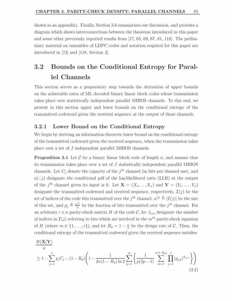
CHAPTER 3. PARITY-CHECK DENSITY: PARALLEL CHANNELS 85
shown in an appendix). Finally, Section 3.6 summarizes our discussion, and presents a
diagram which shows interconnections between the theorems introduced in this paper
and some other previously reported results from [17, 65, 69, 67, 81, 118]. The prelim-
inary material on ensembles of LDPC codes and notation required for this paper are
introduced in [74] and [118, Section 2].
3.2 Bounds on the Conditional Entropy for Paral-
lel Channels
This section serves as a preparatory step towards the derivation of upper bounds
on the achievable rates of ML decoded binary linear block codes whose transmission
takes place over statistically independent parallel MBIOS channels. To this end, we
present in this section upper and lower bounds on the conditional entropy of the
transmitted codeword given the received sequence at the output of these channels.
3.2.1 Lower Bound on the Conditional Entropy
We begin by deriving an information-theoretic lower bound on the conditional entropy
of the transmitted codeword given the received sequence, when the transmission takes
place over a set of J independent parallel MBIOS channels.
Proposition 3.1 Let C be a binary linear block code of length n, and assume that
its transmission takes place over a set of J statistically independent parallel MBIOS
channels. Let Cj denote the capacity of the jth channel (in bits per channel use), and
a(·; j) designate the conditional pdf of the log-likelihood ratio (LLR) at the output
of the jth channel given its input is 0. Let X = (X1, . . .Xn) and Y = (Y1, . . . , Yn)
designate the transmitted codeword and received sequence, respectively, I(j) be the
set of indices of the code bits transmitted over the jth channel, n[j] , |I(j)| be the size
of this set, and pj , n[j]
nbe the fraction of bits transmitted over the jth channel. For
an arbitrary c×n parity-check matrix H of the code C, let βj,m designate the number
of indices in I(j) referring to bits which are involved in the mth parity-check equation
of H (where m ∈ 1, . . . , c), and let Rd = 1 − cn
be the design rate of C. Then, the
conditional entropy of the transmitted codeword given the received sequence satisfies
H(X|Y)
n
≥ 1−J∑
j=1
pjCj − (1−Rd)
(1− 1
2n(1 − Rd) ln 2
∞∑
p=1
1
p(2p−1)
n(1−Rd)∑
m=1
J∏
j=1
(gj,p)βj,m
)
(3.2)

CHAPTER 3. PARITY-CHECK DENSITY: PARALLEL CHANNELS 86
where
gj,p ,
∫ ∞
0
a(l; j) (1 + e−l) tanh2p
(l
2
)dl, j ∈ 1, . . . , J, p ∈ N. (3.3)
Remark 3.1 Note that the input vector X is chosen uniformly from the codewords
of a binary linear block code. Each input bit Xi therefore either gets the values 0
or 1 with probability 12
or is set to zero (due to the linearity of the code). In the
following proof, we assume that all the code symbols get the values 0 or 1 with equal
probability. By slightly modifying the proof, it is simple to show that the bound also
holds for the other case where some of the code bits are set to zero.
Proof: The proof relies on concepts which are presented in [17, 118], and generalizes
them to the case of parallel channels. If a symbol is transmitted over the jth MBIOS
channel and y is the corresponding output, then the LLR gets the form
LLR(y; j) = ln
(p(y|0; j)
p(y|1; j)
), j ∈ 1, . . . , J, y ∈ Y
where Y denotes the output alphabet of each component channel,1 and p(·|·; j) is the
conditional pdf of the jth channel. For each one of these J component channels, we
move from the original mapping of X → Y (where according to (3.1), each symbol
is transmitted over only one of these J channels) to an equivalent representation of
the channel X → Y , where Y represents the LLR of the channel output Y . These
channels are equivalent in the sense that H(X|Y ) = H(X|Y ). The basic idea for
showing the equivalence between the original set of parallel channels and the one
which will be introduced shortly is based on the principle that the LLR forms a
sufficient statistics of an MBIOS channel.
In the following, we characterize an equivalent channel to each of the J parallel
channels. The output of the equivalent channel is defined to be Y , (Φ, Ω). For the
j-th channel, Y is calculated from Y as follows:
Ω , |LLR(Y ; j)|, Φ ,
0 if LLR(Y ; j) > 0
1 if LLR(Y ; j) < 0
0 or 1 w.p. 12
if LLR(Y ; j) = 0
.
Due to the symmetry of the communication channel, the equivalent channel can be
seen as a channel with additive noise where the transmitted signal affects only the Φ
component of the output Y . The characterization of the equivalent channel in this
1In case the output alphabets of the component channels are not equal, then Y can be definedas their union.

CHAPTER 3. PARITY-CHECK DENSITY: PARALLEL CHANNELS 87
form is used for the continuation of this proof and is presented below. For each index
i ∈ I(j), let us choose independently a value Li according to the conditional pdf
a(·; j), and for i ∈ 1, . . . , n, let
Ωi , |Li|, Θi ,
0 if Li > 0
1 if Li < 0
0 or 1 w.p. 12
if Li = 0
.
The output of the set of equivalent channels is defined as Y = (Y1, . . . , Yn) where
Yi = (Φi, Ωi) and Φi = Θi + Xi where the addition is modulo 2. This defines the
mapping
X → Y = (Φ, Ω)
where Φ is a binary random variable which is affected by X, and Ω is a non-negative
random variable which is independent of X. Note that due to the symmetry of
the parallel channels, for each index i ∈ I(j), the joint distribution of (Φi, Ωi) is
independent of i, and is equal to the distribution of the pair representing the sign and
magnitude of LLR(Y ; j). Hence,
fΩi(ω) , fΩ(ω; j) =
a(ω; j) + a(−ω; j) = (1 + e−ω) a(ω; j) if ω > 0
a(0; j) if ω = 0(3.4)
where we rely on the symmetry property of a(·; j).Denoting by R the rate of the code C, since the codewords are transmitted with
equal probability
H(X) = nR. (3.5)
Also, since the J parallel channels are memoryless, then
H(Y|X) =
n∑
i=1
H(Yi|Xi). (3.6)
The mapping Yi → Yi is memoryless, hence H(Y|Y) =∑n
i=1 H(Yi|Yi), and
H(Y) = H(Y) − H(Y|Y) + H(Y|Y)
= H(Y) −n∑
i=1
H(Yi|Yi) + H(Y|Y) (3.7)
H(Y|Y) ≤n∑
i=1
H(Yi|Yi)
=
n∑
i=1
[H(Yi) − H(Yi) + H(Yi|Yi)
]. (3.8)

CHAPTER 3. PARITY-CHECK DENSITY: PARALLEL CHANNELS 88
Applying the above towards the derivation of a lower bound on the conditional entropy
H(X|Y), we get
H(X|Y) = H(X) + H(Y|X) − H(Y)
(a)= nR +
n∑
i=1
H(Yi|Xi) − H(Y) − H(Y|Y) +n∑
i=1
H(Yi|Yi)
(b)
≥ nR +
n∑
i=1
H(Yi|Xi) − H(Y) −n∑
i=1
[H(Yi) − H(Yi) + H(Yi|Yi)
]
+n∑
i=1
H(Yi|Yi)
= nR − H(Y) +
n∑
i=1
H(Yi) −n∑
i=1
[H(Yi) − H(Yi|Xi)
]
= nR − H(Y) +
n∑
i=1
H(Yi) −n∑
i=1
I(Xi; Yi)
(c)
≥ nR − H(Y) +
n∑
i=1
H(Yi) −J∑
j=1
n[j] Cj (3.9)
where (a) relies on (3.5)–(3.7), (b) relies on (3.8), and (c) follows since I(Xi; Yi) ≤ Cj
for all i ∈ I(j), and |I(j)| = n[j] for j ∈ 1, . . . , J. In order to obtain a lower bound
on H(X|Y) from (3.9), we calculate the entropy of the random variables Yi, and
find an upper bound on the entropy of the random vector Y. This finally provides the
lower bound on the conditional entropy given in (3.2). Considering an index i ∈ I(j)
for some j ∈ 1, 2, . . . J, we get
H(Yi) = H(Φi, Ωi)
= H(Ωi) + H(Φi|Ωi)
= H(Ωi) + Eω [H(Φi|Ωi = ω)]
= H(Ωi) + 1 (3.10)
where the last transition is due to the fact that given the absolute value of the LLR,
since the parallel channels are MBIOS and the coded bits are equally likely to be 0 or
1, the sign of the LLR is equally likely to be positive or negative. The entropy H(Ωi)
is not expressed explicitly as it cancels out later.
We now turn to derive an upper bound on H(Y):
H(Y) = H((Φ1, . . . , Φn), (Ω1, . . . , Ωn)
)
= H(Ω1, . . . , Ωn) + H((Φ1, . . . , Φn) | (Ω1, . . . , Ωn)
)
=
n∑
i=1
H(Ωi) + H((Φ1, . . . , Φn) | (Ω1, . . . , Ωn)
)(3.11)

CHAPTER 3. PARITY-CHECK DENSITY: PARALLEL CHANNELS 89
where the last equality follows since the random variables Ωi are statistically inde-
pendent.
Define the c-dimensional syndrome vector as
S , (Φ1, . . . , Φn) HT
where H is a c×n parity-check matrix of the binary linear block code C, and let L be
the index of the vector (Φ1, . . . , Φn) in the coset which corresponds to S. Since each
coset has exactly 2nR elements which are equally likely then H(L) = nR, and we get
H((Φ1, . . . , Φn) | (Ω1, . . . , Ωn)
)= H
(S, L | (Ω1, . . . , Ωn)
)
≤ H(L) + H(S | (Ω1, . . . , Ωn)
)
= nR + H(S | (Ω1, . . . , Ωn)
)
≤ nR +c∑
m=1
H(Sm | (Ω1, . . . , Ωn)
). (3.12)
Since XHT = 0 for any codeword, then
S = (Θ1, . . . , Θn) HT .
Let us consider the mth parity-check equation which involves km variables, and assume
that the set of indices of these variables is i1, . . . , ikm. Then, the component Sm
of the syndrome is equal to 1 if and only if there is an odd number of ones in the
random vector (Θi1, . . . , Θikm). To calculate the probability that Sm is equal to 1, we
rely on the following lemma:
Lemma 3.1 ([118], Lemma 4.1) If the mth linear constraint defined by the parity-
check matrix H involves km variables, and if i1, . . . , ikm denote the indices of these
variables, then
Pr(Sm = 1 | (Ωi1, . . . , Ωikm
) = (α1, . . . , αkm))
=1
2
[1 −
km∏
w=1
tanh(αw
2
)]. (3.13)
From this lemma, we obtain
H(Sm|(Ωi1 , . . . , Ωikm
) = (α1, . . . , αkm))
= h2
(1
2
[1 −
km∏
w=1
tanh(αw
2
)])
where h2 denotes the binary entropy function to base 2. By taking the statistical
expectation over the km random variables Ωi1 , . . . , Ωikm, we get
H(Sm|(Ωi1 , . . . , Ωikm
))
=
∫ ∞
0
. . .
∫ ∞
0
h2
(1
2
[1 −
km∏
w=1
tanh(αw
2
)]) km∏
w=1
fΩiw(αw) dα1dα2 . . . dαkm
.

CHAPTER 3. PARITY-CHECK DENSITY: PARALLEL CHANNELS 90
Let βj,m denote the number of indices w ∈ i1, . . . , ikm referring to variables which
are transmitted over the jth channel. From the Taylor series expansion of the binary
entropy function (h2) around x = 12
(see [118, Appendix B.1])
h2(x) = 1 − 1
2 ln 2
∞∑
p=1
(1 − 2x)2p
p(2p − 1), 0 ≤ x ≤ 1 (3.14)
it follows that
H(Sm|(Ωi1 , . . . , Ωikm
))
= 1 − 1
2 ln 2
∞∑
p=1
1
p(2p − 1)
km∏
w=1
(∫ ∞
0
fΩiw(α) tanh2p
(α
2
)dα
)
= 1 − 1
2 ln 2
∞∑
p=1
1
p(2p − 1)
J∏
j=1
(∫ ∞
0
fΩ(α; j) tanh2p(α
2
)dα
)βj,m
(3.15)
where the first transition is based on (3.14) and follows along the same lines as [118,
Appendix B.2]), and the second transition is due to the fact that for all i ∈ I(j), the
pdf of the random variable Ωi is independent of i, see (3.4). Summing over all the
parity-check equations of H gives
c∑
m=1
H(Sm|(Ω1, . . . , Ωn)
)
= c − 1
2 ln 2
∞∑
p=1
1
p(2p − 1)
c∑
m=1
J∏
j=1
(∫ ∞
0
fΩ(α; j) tanh2p(α
2
)dα
)βj,m
. (3.16)
By combining (3.4), (3.11), (3.12) and (3.16), we get the following upper bound on
H(Y):
H(Y) ≤n∑
i=1
H(Ωi) + nR + c
[1 − 1
2c ln 2
∞∑
p=1
1
p(2p − 1)
·c∑
m=1
J∏
j=1
(∫ ∞
0
a(α; j)(1 + e−α) tanh2p(α
2
)dα
)βj,m
]
(a)=
n∑
i=1
H(Ωi) + nR + n(1 − Rd)
·[1 − 1
2n(1 − Rd) ln 2
∞∑
p=1
1
p(2p − 1)
c∑
m=1
J∏
j=1
gj,pβj,m
](3.17)
where (a) relies on the definition of gj,p in (3.3) and since Rd , 1 − cn
denotes the
design rate of C. Finally, the substitution of (3.10) and (3.17) in the RHS of (3.9)

CHAPTER 3. PARITY-CHECK DENSITY: PARALLEL CHANNELS 91
provides the lower bound on the conditional entropy H(X|Y) given in (3.2). This
completes the proof of the proposition.
3.2.2 Upper Bound on the Conditional Entropy
In this section, we provide an upper bound on the conditional entropy of the transmit-
ted codeword given the received sequence. The bound holds for an arbitrary binary
linear block code whose transmission takes place over a set of parallel channels, and
is expressed in terms of the code rate and the bit-error probability of the code (under
ML decoding or a sub-optimal decoding algorithm).
Lemma 3.2 Let C be a binary linear block code of length n and rate R, and assume
that its transmission takes place over a set of parallel channels. Let X = (X1, . . . , Xn)
and Y = (Y1, . . . , Yn) designate the transmitted codeword and the received sequence,
respectively. ThenH(X|Y)
n≤ R h2(Pb) (3.18)
where Pb designates the bit error probability of the code C under an arbitrary decoding
algorithm.
Proof: Since there is a one to one correspondence between the codewords and the
set of information bits used to encode them, then H(X|Y) = H(U|Y) where the
vector U = (U1, . . . , UnR) denotes the sequence of information bits used to encode
the codeword X. Let P(i)b (C) denote the probability of decoding the bit Ui erroneously
given the received sequence at the output of the set of parallel channels, then the bit
error probability is given by
Pb(C) =1
nR
nR∑
i=1
P(i)b (C). (3.19)
This therefore gives
H(X|Y)
n=
H(U|Y)
n(a)
≤ 1
n
nR∑
i=1
H(Ui|Y)
(b)
≤ 1
n
nR∑
i=1
h2
(P
(i)b (C)
)
(c)
≤ R h2
(1
nR
nR∑
i=1
P(i)b (C)
)
(d)= R h2
(Pb(C)
)

CHAPTER 3. PARITY-CHECK DENSITY: PARALLEL CHANNELS 92
where inequality (a) holds from the chain rule of entropy and since conditioning
reduces entropy, inequality (b) follows from Fano’s inequality and since the code is
binary, inequality (c) is based on Jensen’s inequality and the concavity of the binary
entropy function, and equality (d) follows from (3.19).
3.3 An Upper Bound on the Achievable Rates of
LDPC codes over Parallel Channels
In this section, we derive an upper bound on the design rate of a sequence of ensembles
of LDPC codes whose transmission takes place over a set of statistically independent
parallel MBIOS channels, and which achieves vanishing bit error probability under
ML decoding. This bound is used in the next section for the derivation of an upper
bound on the design rate of an arbitrary sequence of ensembles of punctured LDPC
codes.
Let us assume that a binary LDPC code C of length n is transmitted over a set
of J statistically independent parallel MBIOS channels. Denote the number of code
bits of C which are transmitted over the jth channel by n[j], and the fraction of bits
transmitted over the jth channel by
pj ,n[j]
n, j ∈ 1, . . . , J. (3.20)
Let G be a bipartite graph which represents the code C, and E be the set of edges in
G. Let E[j] designate the set of edges connected to variable nodes which correspond
to code bits transmitted over the jth channel, and
qj ,|E[j]||E| , j ∈ 1, . . . , J (3.21)
denote the fraction of edges connected to these variable nodes. Referring to the edges
from the subset E[j], let λ[j]i designate the fraction of these edges which are connected
to variable nodes of degree i, and define the following J degree distributions from the
edge perspective:
λ[j](x) ,
∞∑
i=2
λ[j]i xi−1 , j ∈ 1, . . . , J
which correspond to each of the J parallel channels. According to this notation, the
number of edges connected to variable nodes corresponding to code bits transmitted

CHAPTER 3. PARITY-CHECK DENSITY: PARALLEL CHANNELS 93
over the jth channel is given by
|E[j]| =n[j]
∞∑
i=2
λ[j]i
i
, j ∈ 1, . . . , J. (3.22)
For the simplicity of the notation, let us define a vector of degree distributions for the
variable nodes from the edge perspective to be λ(x) =(λ[1](x), . . . , λ[J ](x)
). Following
the notation in [69], the ensemble (n, λ, ρ) is defined to be the set of LDPC codes
of length n, which according to their representation by bipartite graphs and the
assignment of their code bits to the parallel channels, imply left and right degree
distributions of λ and ρ, respectively.
Lemma 3.31
∫ 1
0λ(x) dx
=
J∑
j=1
pj∫ 1
0λ[j](x) dx
. (3.23)
where λ is the overall left degree distribution which serves to construct the vector of
left degree distributions λ by considering the assignments of variables nodes to the
different channels.
Proof: Since E[1], . . . , E[J ] forms a sequence of disjoint sets whose union is the set
E, we get the equality |E| =∑J
j=1 |E[j]|. From (3.22), we therefore get
n∑∞i=2
λi
i
=J∑
j=1
n[j]
∑∞i=2
λ[j]i
i
(3.24)
and by dividing both sides of the equality by n and using (3.20), the lemma follows
immediately.
Lemma 3.4
qj =pj∫ 1
0λ[j](x) dx
· 1J∑
k=1
pk∫ 1
0λ[k](x) dx
, ∀ j ∈ 1, . . . , J. (3.25)
Proof: The lemma follows directly from (3.21), (3.22) and Lemma 3.3.
In the following, we introduce a sequence of ensembles of LDPC codes, say
(nr, λr, ρ)∞r=1 where all the codes in each ensemble have the same number of bits
assigned to each of the J parallel channels, and ρ is fixed for all the ensembles of

CHAPTER 3. PARITY-CHECK DENSITY: PARALLEL CHANNELS 94
this sequence (i.e., it is independent of r). Since λ which corresponds to the overall
left degree distribution of the edges is also independent of r, one can consider here
the common design rate of the sequence of ensembles (nr, λr, ρ)∞r=1 which does not
depend on r.
This setting is general enough for applying the following theorem to various ap-
plications which form particular cases of communication over parallel channels, e.g.,
punctured LDPC codes [35, 39], non-uniformly error protected LDPC codes [69], and
LDPC-coded modulation (see e.g., [37, 112]). In this setting, the fraction of code bits
assigned to the jth channel, pj,r, depends on j ∈ 1, . . . , J and r ∈ N, but not on
the particular code chosen from each ensemble. It follows from Lemma 3.4 that the
same property also holds for qj,r which designates the fraction of edges connected to
variable nodes whose code bits are assigned to the jth channel. In the following, we
assume that the limits
pj , limr→∞
pj,r, qj , limr→∞
qj,r (3.26)
exist and we also assume that they are positive for all j ∈ 1, . . . , J (though in
general, they are non-negative).
Theorem 3.1 Let a sequence of LDPC ensembles (nr, λr, ρ)∞r=1 be transmitted
over a set of J statistically independent parallel MBIOS channels, and assume that
the block length (nr) goes to infinity as we let r tend to infinity. Let Cj denote the
capacity of the jth channel, and a(·; j) designate the pdf of the LLR at the output
of the jth channel given its input is 1. If in the limit where r tends to infinity, the
bit error probability of this sequence under ML decoding vanishes, then the common
design rate Rd of these ensembles satisfies
Rd ≤ 1 −1 −
J∑
j=1
pjCj
1 − 1
2 ln 2
∞∑
p=1
1
p(2p − 1)Γ
( J∑
j=1
qj gj,p
) (3.27)
where Γ denotes the right degree distribution from the node perspective, and gj,p is
introduced in (3.3).
Proof: Let Cr∞r=1 be a sequence of LDPC codes chosen uniformly at random from
the sequence of ensembles (nr, λr, ρ)∞r=1. Denote the rate of the code Cr by Rr, and
let Pb,r be its bit error probability under ML decoding. Let Gr be a bipartite graph
of the code Cr whose left and right degree distributions from the edge perspective
are λr and ρ, respectively. From Proposition 3.1 and Lemma 3.2, it follows that the

CHAPTER 3. PARITY-CHECK DENSITY: PARALLEL CHANNELS 95
following inequality holds for the binary linear block code Cr:
Rrh2(Pb,r) ≥ 1 −J∑
j=1
pj,rCj − (1 − Rd)
·
1 − 1
2nr(1 − Rd) ln 2
∞∑
p=1
1
p(2p − 1)
nr(1−Rd)∑
m=1
J∏
j=1
(gj,p)βr,j,m
(3.28)
where nr is the block length of the code Cr, Rd is the common design rate for
all the codes from the sequence of ensembles (nr, λr, ρ)∞r=1, and βr,j,m denotes the
number of edges which are connected to the mth parity-check node of the graph Gr
and are related to code bits transmitted over the jth channel (where j ∈ 1, . . . , Jand m ∈ 1, . . . nr(1 − Rd)). By taking the expectation on both sides of (3.28) and
letting r tend to infinity, we get
1 −J∑
j=1
pjCj − (1 − Rd) limr→∞
(1 − 1
2nr(1 − Rd) ln 2
·∞∑
p=1
1
p(2p − 1)
nr(1−Rd)∑
m=1
E
(J∏
j=1
(gj,p)βr,j,m
)
≤ 0. (3.29)
The RHS of (3.29) follows from the LHS of (3.28), due to the concavity of the binary
entropy function and Jensen’s inequality, and since by our assumption, the bit error
probability of the ensembles vanishes in the limit where r tends to infinity.
The derivation of an upper bound on the design rate is proceeded by calculating
the expectation of the product inside the LHS of (3.29). Let kr,m denote the degree
of the mth parity-check node of the bipartite graph Gr, then the smoothing theorem
gives
E
(J∏
j=1
(gj,p)βr,j,m
)= E
[E
(J∏
j=1
(gj,p)βr,j,m
∣∣∣J∑
j=1
βr,j,m = kr,m
)](3.30)
where the outer expectation is carried over the random variable kr,m. We first cal-
culate the inner expectation in the RHS of (3.30). It follows from (3.22) that the
number of edges, |E[j]r | , |E[j](Gr)|, connected to variable nodes corresponding to
code bits transmitted over the jth channel, is independent of the code Cr choosen
from the ensemble (nr, λr, ρ). The same property also holds for the total number of
edges in the graph (since |Er| =∑J
j=1 |E[j]r |). Since the code Cr is chosen uniformly
at random from the ensemble, it follows that if kr,m is a given positive integer, then

CHAPTER 3. PARITY-CHECK DENSITY: PARALLEL CHANNELS 96
E
(J∏
j=1
(gj,p)βr,j,m
∣∣∣J∑
j=1
βr,j,m = kr,m
)
=∑
b1, . . . , bJ ≥ 0PJj=1
bj = kr,m
Pr(βr,j,m = bj , ∀j ∈ 1, . . . , J
) J∏
j=1
(gj,p)bj
=∑
b1, . . . , bJ ≥ 0PJj=1
bj = kr,m
(|E[1]r |b1
)· · ·(|E[J]
r |bJ
)( |Er|
kr,m
)J∏
j=1
(gj,p)bj
. (3.31)
Lemma 3.5
limr→∞
(|E[1]r |b1
)· · ·(|E[J]
r |bJ
)( |Er|
kr,m
) =J∏
j=1
(qj)bj lim
r→∞
(kr,m
b1, b2, . . . , bJ
). (3.32)
Proof: By assumption, in the limit where we let r tend to infinity, the block length
nr also tends to infinity. Hence, from (3.22) and the assumption that qj > 0 for every
j ∈ 1, . . . , J, we get that for all j ∈ 1, . . . , J, E[j]r approaches infinity in the limit
where r tends to infinity.
limr→∞
(|E[1]r |
b1
)· · ·(|E[J]
r |bJ
)( |Er|
kr,m
)
= limr→∞
|E[1]r |! · · · |E[J ]
r |!|Er|!
(|Er| − kr,m)!
(|E[1]r | − b1)! · · · (|E[J ]
r | − bJ)!
(kr,m
b1, b2, . . . , bJ
)
= limr→∞
|E[1]
r |! · · · |E[J ]r |!
|Er|!(|Er| − kr,m)!
(|E[1]r | − b1)! . . . (|E[J ]
r | − bJ )!
limr→∞
(kr,m
b1, b2, . . . , bJ
)
(a)= lim
r→∞
|E[1]r |b1 · · · |E[J ]
r |bJ
|Er|kr,mlimr→∞
(kr,m
b1, b2, . . . , bJ
)
(b)= lim
r→∞
(|E[1]
r ||Er|
)b1
. . .
(|E[J ]
r ||Er|
)bJ
limr→∞
(kr,m
b1, b2, . . . , bJ
)
(c)= lim
r→∞
J∏
j=1
(qj,r)bj lim
r→∞
(kr,m
b1, b2, . . . , bJ
)
=
J∏
j=1
(qj)bj lim
r→∞
(kr,m
b1, b2, . . . , bJ
)
where equality (a) follows since for all j ∈ 1, . . . , J, |E[j]r | → ∞ as we let r tend to
infinity, while on the other hand, the maximal right degree (and hence, also b1, . . . , bJ

CHAPTER 3. PARITY-CHECK DENSITY: PARALLEL CHANNELS 97
and kr,m) stay bounded; equality (b) is valid due to the constraint∑J
j=1 bj = kr,m,
and equality (c) follows from (3.21).
By letting r tend to infinity on both sides of (3.30), and substituting (3.31) and
(3.32) in the RHS of (3.30), we get that for all p ∈ N
limr→∞
E
[J∏
j=1
(gj,p)βr,j,m
]
(a)= E
[limr→∞
E
(J∏
j=1
(gj,p)βr,j,m
∣∣∣J∑
j=1
βr,j,m = kr,m
)]
(b)= E
[limr→∞
∑
b1, . . . , bJ ≥ 0PJj=1
bj = kr,m
(kr,m
b1, b2, . . . , bJ
) J∏
j=1
(qj gj,p)bj
]
= E
[limr→∞
(J∑
j=1
qjgj,p
)kr,m]
(c)=
dc,max∑
k=1
Γk
( J∑
j=1
qjgj,p
)k
= Γ
( J∑
j=1
qjgj,p
)(3.33)
where equality (a) follows from (3.30) and since the right degree distribution is inde-
pendent of r (note that the outer expectation in equality (a) is performed w.r.t. the
degree of the mth parity-check node); equality (b) follows from (3.31) and (3.32), and
since the number of terms in the sum is bounded (this number is upper bounded by
(kr,m)J−1, so it is bounded for all r ∈ N due to the fact that the maximal right degree
is fixed), and equality (c) follows since the right degree distribution is independent
of r. Since the limit in (3.33) does not depend on the index m which appears in the
inner summation at the LHS of (3.29) and also limr→∞ nr(1−Rd) = ∞, then we get
from (3.33)
limr→∞
1
nr(1 − Rd)
nr(1−Rd)∑
m=1
E
[J∏
j=1
(gj,p)βr,j,m
]
(a)= lim
r→∞E
[J∏
j=1
(gj,p)βr,j,m
]
(b)= Γ
( J∑
j=1
qjgj,p
)(3.34)

CHAPTER 3. PARITY-CHECK DENSITY: PARALLEL CHANNELS 98
where equality (a) follows from the fact that if ar is a convergent sequence then
the equality limr→∞1r
∑ri=1 ai = limr→∞ ar holds, and also since any sub-sequence
of a convergent sequence converges to the same limit as of the original sequence;
equality (b) follows from (3.33). Combining (3.29) and (3.34) gives
1 −J∑
j=1
pjCj − (1 − Rd)
(1 − 1
2 ln 2
∞∑
p=1
1
p(2p − 1)Γ
( J∑
j=1
qjgj,p
))≤ 0.
Finally, solving the last inequality for Rd gives the upper bound on the design rate
in (3.27).
Example 3.1 For the special case where the J parallel MBIOS channels are binary
erasure channels where the erasure probability of the jth channel is εj, we get from
(3.3)
gj,p = 1 − εj , ∀ j ∈ 1, . . . , J, p ∈ N. (3.35)
Since gj,p is independent of p for a BEC, and based on the equality∑∞
p=11
2p(2p−1)= ln 2,
we obtain from Theorem 3.1 that the common design rate of the sequence of LDPC
ensembles is upper bounded by
Rd ≤ 1 −
J∑
j=1
pjεj
1 − Γ
(1 −
J∑
j=1
qj εj
) . (3.36)
This result coincides with [69, Theorem 2].
The proof of Theorem 3.1 relies on the assumption that the right degree distribu-
tion ρ is fixed, and does not depend on the ordinal number r of the ensemble. For a
capacity-achieving sequence of LDPC ensembles, both the maximal and the average
right degrees tend to infinity (see [81, Theorem 1]). Hence, for a capacity-achieving
sequence of LDPC codes, ρ cannot be fixed.
Remark 3.2 One can think of Lemma 3.5 in terms of drawing colored balls from
an urn (where the colors are determined in one to one correspondence with the as-
signments of the various edges to the component channels). Since an edge can only
be assigned once to a parity-check node, the balls are not returned to the urn after
they are chosen. As the block length tends to infinity, so does the number of edges
originating in each of the parallel channels (this is the reason for requiring that qj
is positive for all j). Since the degree of the parity-check nodes remains finite, we
are drawing a finite number of balls from an urn which contains an infinite number
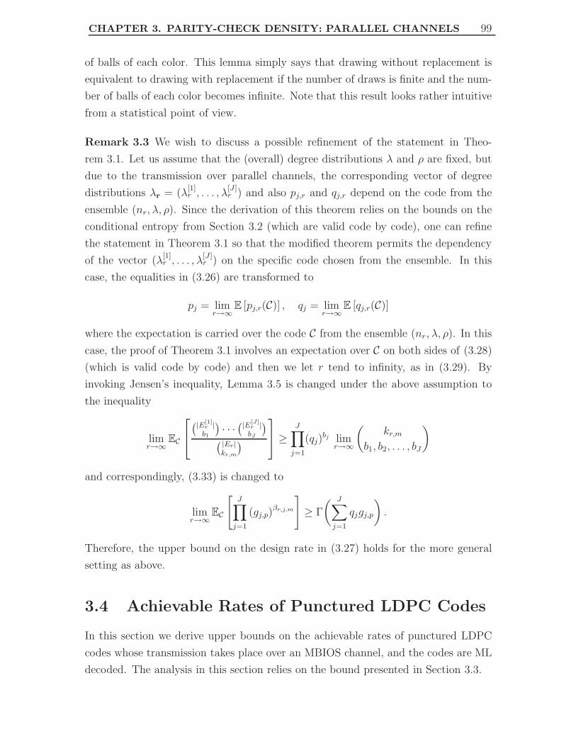
CHAPTER 3. PARITY-CHECK DENSITY: PARALLEL CHANNELS 99
of balls of each color. This lemma simply says that drawing without replacement is
equivalent to drawing with replacement if the number of draws is finite and the num-
ber of balls of each color becomes infinite. Note that this result looks rather intuitive
from a statistical point of view.
Remark 3.3 We wish to discuss a possible refinement of the statement in Theo-
rem 3.1. Let us assume that the (overall) degree distributions λ and ρ are fixed, but
due to the transmission over parallel channels, the corresponding vector of degree
distributions λr = (λ[1]r , . . . , λ
[J ]r ) and also pj,r and qj,r depend on the code from the
ensemble (nr, λ, ρ). Since the derivation of this theorem relies on the bounds on the
conditional entropy from Section 3.2 (which are valid code by code), one can refine
the statement in Theorem 3.1 so that the modified theorem permits the dependency
of the vector (λ[1]r , . . . , λ
[J ]r ) on the specific code chosen from the ensemble. In this
case, the equalities in (3.26) are transformed to
pj = limr→∞
E [pj,r(C)] , qj = limr→∞
E [qj,r(C)]
where the expectation is carried over the code C from the ensemble (nr, λ, ρ). In this
case, the proof of Theorem 3.1 involves an expectation over C on both sides of (3.28)
(which is valid code by code) and then we let r tend to infinity, as in (3.29). By
invoking Jensen’s inequality, Lemma 3.5 is changed under the above assumption to
the inequality
limr→∞
EC
(|E[1]
r |b1
)· · ·(|E[J]
r |bJ
)( |Er|
kr,m
)
≥J∏
j=1
(qj)bj lim
r→∞
(kr,m
b1, b2, . . . , bJ
)
and correspondingly, (3.33) is changed to
limr→∞
EC
[J∏
j=1
(gj,p)βr,j,m
]≥ Γ
( J∑
j=1
qjgj,p
).
Therefore, the upper bound on the design rate in (3.27) holds for the more general
setting as above.
3.4 Achievable Rates of Punctured LDPC Codes
In this section we derive upper bounds on the achievable rates of punctured LDPC
codes whose transmission takes place over an MBIOS channel, and the codes are ML
decoded. The analysis in this section relies on the bound presented in Section 3.3.

CHAPTER 3. PARITY-CHECK DENSITY: PARALLEL CHANNELS 100
Let C be a binary linear block code. Assume its code bits are partitioned into J
disjoint sets, and the bits of the jth set are randomly punctured with a puncturing
rate πj (where j ∈ 1, . . . , J). The transmission of this code over an MBIOS channel
is equivalent to transmitting the code over a set of J parallel MBIOS channels where
each of these channels forms a serial concatenation of a BEC whose erasure probability
is equal to the puncturing rate πj , followed by the original MBIOS channel (see e.g.,
[35, 65, 68, 69]).
3.4.1 Some Preparatory Lemmas
This sub-section presents two lemmas which are later used to prove results for ensem-
bles of randomly and intentionally punctured LDPC codes (denoted by RP-LDPC
and IP-LDPC codes, respectively).
In the following lemma, we consider a punctured linear block code and provide
an upper bound on the conditional entropy of a codeword before puncturing, given
the received sequence at the output of the channel. This upper bound is expressed
in terms of the bit error probability of the punctured code.
Lemma 3.6 Let C′ be a binary linear block code of length n and rate R′, and let C be
a code which is obtained from C′ by puncturing some of its code bits. Assume that the
transmission of the code C takes place over an arbitrary communication channel, and
the code is decoded by an arbitrary decoding algorithm. Let X′ = (X ′1, . . . , X
′n) and
Y = (Y1, . . . , Yn) (where the punctured bits are replaced by question marks which
have an LLR of zero) designate the transmitted codeword of C′ and the received
sequence, respectively. Then, the conditional entropy of the original codeword of C′
given the received sequence satisfies
H(X′|Y)
n≤ R′ h2(Pb) (3.37)
where Pb designates the bit error probability of the punctured code C.
Proof: The proof follows directly from Lemma 3.2, and the equivalence between the
transmission of punctured codes over an MBIOS channel and the special case of trans-
mitting these codes over a set of parallel channels (see the introductory paragraph of
Section 3.4).
Puncturing serves to increase the rate of the original code by reducing the length of
the codeword. It may however cause several codewords to be mapped onto a single
codeword, thereby reducing the dimension of the code. Consider a binary linear code,
C′, of length n and rate R′ and assume a fraction γ of its code bits are punctured. In

CHAPTER 3. PARITY-CHECK DENSITY: PARALLEL CHANNELS 101
the case that the dimension is not reduced by puncturing, the rate of the punctured
code is given by R = R′
1−γ. In the general case, we cannot guarantee that the dimension
of the code is not reduced. However, for a sequence of punctured codes whose bit error
probability vanishes as the block length of the codes tends to infinity, the following
lemma shows that the rate of the punctured codes converges to the desired rate R.
Lemma 3.7 Let C′r be a sequence of binary linear block codes of length nr and rate
R′r, and let Cr be a sequence of codes which is obtained from C′
r by puncturing
a fraction γ of the code bits. Assume the sequence of punctured codes Cr achieves
vanishing bit error probability in the limit where we let r tend to infinity. Then, the
asymptotic rate R of the sequence of punctured codes is given by
R =R′
1 − γ(3.38)
where R′ = limr→∞ R′r is the asymptotic rate of the original sequence of codes C′
r.
Proof: Let X′r = (X ′
1, . . . , X′nr
) and Yr = (Yr . . . , Ynr) designate the original code-
word (before puncturing) and the received sequence (after puncturing), respectively.
Since we assume the there exists a decoding algorithm such that the punctured codes
achieve vanishing bit error probability, we have from lemma 3.6 that
limr→∞
H(X′r|Yr)
nr
= 0.
Let Xr = (X1, . . . , Xnr) designate the codeword after puncturing (where the punc-
tured bits are replaced by question marks). Since X′r ⇒ Xr ⇒ Yr forms a Markov
chain, then by the information processing inequality, we get H(X′r|Xr) ≤ H(X′
r|Yr).
The non-negativity of the conditional entropy therefore yields that
limr→∞
H(X′r|Xr)
nr
= 0. (3.39)
Denote the number of dimensions of the codes C′r and Cr by d′
r and dr, respectively.
Since C′r is binary and linear, every codeword of Cr originates from exactly 2d′r−dr
different codewords of C′r. The codewords are assumed to be transmitted with equal
probability, and therefore H(X′r|Xr) = d′
r − dr. Let Rr designate the rate of the
punctured code Cr. By definition, d′r = R′
rnr, and since nr(1 − γ) forms the block
length of the punctured code Cr, then dr = Rrnr(1 − γ). Substituting the last three
equalities into (3.39) gives
limr→∞
(R′r − Rr(1 − γ)) = 0.
This completes the proof of the lemma.
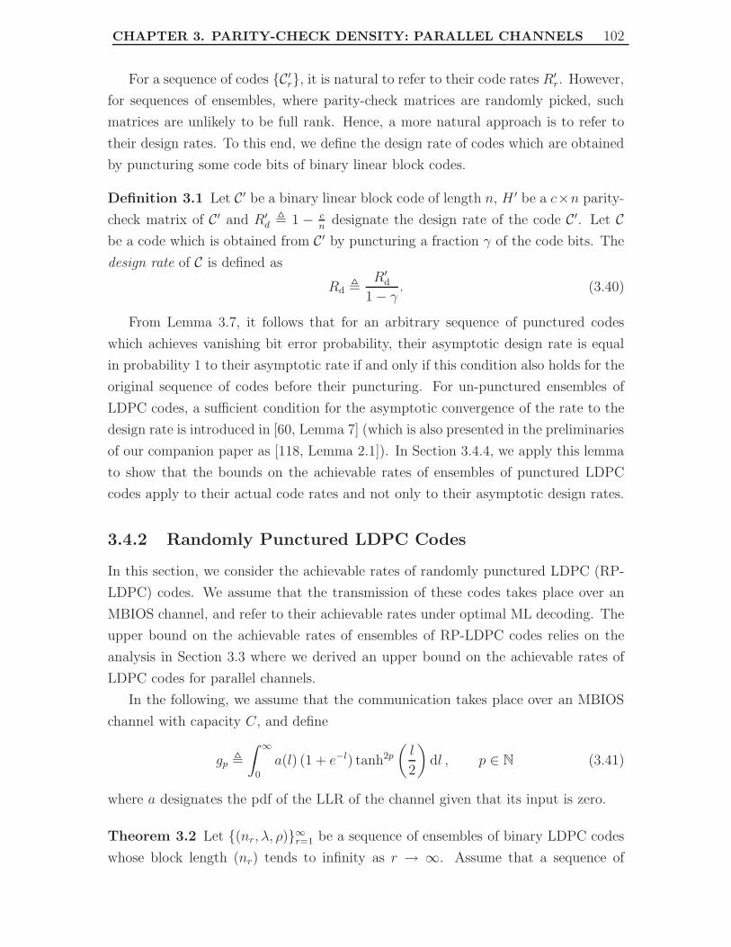
CHAPTER 3. PARITY-CHECK DENSITY: PARALLEL CHANNELS 102
For a sequence of codes C′r, it is natural to refer to their code rates R′
r. However,
for sequences of ensembles, where parity-check matrices are randomly picked, such
matrices are unlikely to be full rank. Hence, a more natural approach is to refer to
their design rates. To this end, we define the design rate of codes which are obtained
by puncturing some code bits of binary linear block codes.
Definition 3.1 Let C′ be a binary linear block code of length n, H ′ be a c×n parity-
check matrix of C′ and R′d , 1 − c
ndesignate the design rate of the code C′. Let C
be a code which is obtained from C′ by puncturing a fraction γ of the code bits. The
design rate of C is defined as
Rd ,R′
d
1 − γ. (3.40)
From Lemma 3.7, it follows that for an arbitrary sequence of punctured codes
which achieves vanishing bit error probability, their asymptotic design rate is equal
in probability 1 to their asymptotic rate if and only if this condition also holds for the
original sequence of codes before their puncturing. For un-punctured ensembles of
LDPC codes, a sufficient condition for the asymptotic convergence of the rate to the
design rate is introduced in [60, Lemma 7] (which is also presented in the preliminaries
of our companion paper as [118, Lemma 2.1]). In Section 3.4.4, we apply this lemma
to show that the bounds on the achievable rates of ensembles of punctured LDPC
codes apply to their actual code rates and not only to their asymptotic design rates.
3.4.2 Randomly Punctured LDPC Codes
In this section, we consider the achievable rates of randomly punctured LDPC (RP-
LDPC) codes. We assume that the transmission of these codes takes place over an
MBIOS channel, and refer to their achievable rates under optimal ML decoding. The
upper bound on the achievable rates of ensembles of RP-LDPC codes relies on the
analysis in Section 3.3 where we derived an upper bound on the achievable rates of
LDPC codes for parallel channels.
In the following, we assume that the communication takes place over an MBIOS
channel with capacity C, and define
gp ,
∫ ∞
0
a(l) (1 + e−l) tanh2p
(l
2
)dl , p ∈ N (3.41)
where a designates the pdf of the LLR of the channel given that its input is zero.
Theorem 3.2 Let (nr, λ, ρ)∞r=1 be a sequence of ensembles of binary LDPC codes
whose block length (nr) tends to infinity as r → ∞. Assume that a sequence of

CHAPTER 3. PARITY-CHECK DENSITY: PARALLEL CHANNELS 103
ensembles of RP-LDPC codes is constructed in the following way: for each code from
an ensemble of the original sequence, a subset of αnr code bits is a-priori selected, and
these bits are randomly punctured at a fixed rate (Ppct). Assume that the punctured
codes are transmitted over an MBIOS channel with capacity C, and that in the limit
where r approaches infinity, the sequence of ensembles of RP-LDPC codes achieves
vanishing bit error probability under some decoding algorithm. Then in probability 1
w.r.t. the random puncturing patterns, the asymptotic design rate (Rd) of the new
sequence satisfies
Rd ≤ 1
1 − αPpct
1 − 1 − (1 − αPpct)C
1 − 1
2 ln 2
∞∑
p=1
1
p(2p − 1)Γ((1 − Ppct + ξ)gp
)
(3.42)
where Γ denotes the right degree distribution (from the node perspective) of the
original sequence, gp is introduced in (3.41), and ξ is the following positive number:
ξ , 2(1 − α)Ppct
∫ 1
0
λ(x) dx. (3.43)
Proof: By assumption, we select a set of code bits whose size is a fraction α of the nr
code bits, and these bits are randomly punctured at rate Ppct. The transmission of the
resulting codeword over an MBIOS channel is equivalent to the transmission of the
original codeword over a set of J = 2 parallel channels. The first channel, referring to
the set of code bits which are randomly punctured, is a serial concatenation of a BEC
with erasure probability Ppct and the original MBIOS channel; the second channel
which refers to the rest of the bits (which are transmitted without being randomly
punctured) is the original MBIOS channel. For simplicity, let us first assume that
the degree distribution associated with the selected subset of αnr code bits which are
randomly punctured is independent of the specific code from the ensemble (nr, λ, ρ).
Based on the discussion above and the notation in Section 3.3, the transmission of
the nr code bits over these two parallel channels induces a sequence of ensembles of
LDPC codes, (nr, λr, ρ)∞r=1, where λr = (λ[1]r , λ
[2]r ) depends on the selection of the
subset of αnr code bits which are randomly punctured. Following this equivalence,
we get from the notation in Theorem 3.1 that
p1 = α, p2 = 1 − α, C1 = C(1 − Ppct), C2 = C
⇒J∑
j=1
pjCj = C(1 − αPpct). (3.44)

CHAPTER 3. PARITY-CHECK DENSITY: PARALLEL CHANNELS 104
In order to apply Theorem 3.1 to our case, we find a global lower bound on the sum∑J
j=1 qjgj,p which does not depend on the a-priori selection of the subset of code bits
which are randomly punctured. From (3.3) and (3.41), it follows that for all p ∈ N:
g1,p =
∫ ∞
0
[Ppctδ(l) + (1 − Ppct)a(l)] (1 + e−l) tanh2p
(l
2
)dl
= (1 − Ppct)
∫ ∞
0
a(l)(1 + e−l) tanh2p
(l
2
)dl
= (1 − Ppct) gp
and g2,p = gp. Based on Lemmas 3.3 and 3.4, we get that for all p ∈ N
q1g1,p + q2g2,p =
αgp(1 − Ppct)
∫ 1
0
λ(x) dx
∫ 1
0
λ[1]r (x) dx
+
(1 − α)gp
∫ 1
0
λ(x)dx
∫ 1
0
λ[2]r (x) dx
(3.45)
where the following constraint is satisfied:
α∫ 1
0
λ[1]r (x) dx
+1 − α
∫ 1
0
λ[2]r (x) dx
=1
∫ 1
0
λ(x) dx
(3.46)
and ∫ 1
0
λ[1]r (x) dx ≤ 1
2,
∫ 1
0
λ[2]r (x) dx ≤ 1
2(3.47)
due to the fact that λ[1](x) ≤ x and λ[2](x) ≤ x for x ∈ [0, 1] (even without explicitly
knowing λ[1] and λ[2] which depend on the a-priori choice of the subset of bits which
are randomly punctured). Based on (3.45)–(3.47), we get
q1g1,p + q2g2,p
= (1 − Ppct)gp
∫ 1
0
λ(x) dx
α∫ 1
0
λ[1]r (x) dx
+1 − α
∫ 1
0
λ[2]r (x) dx
+
(1 − α)Ppctgp
∫ 1
0
λ(x) dx
∫ 1
0
λ[2]r (x) dx
= (1 − Ppct)gp +
(1 − α)Ppctgp
∫ 1
0
λ(x) dx
∫ 1
0
λ[2]r (x) dx
≥(
1 − Ppct + 2(1 − α)Ppct
∫ 1
0
λ(x) dx
)gp
= (1 − Ppct + ξ)gp

CHAPTER 3. PARITY-CHECK DENSITY: PARALLEL CHANNELS 105
where ξ is defined in (3.43). Since the degree distribution Γ is a monotonic increasing
function, then
Γ
(J∑
j=1
qjgj,p
)≥ Γ
((1 − Ppct + ξ)gp
). (3.48)
By substituting (3.44) and (3.48) in the RHS of (3.27), we obtain the following upper
bound on the asymptotic design rate of the original sequence
R′d ≤ 1 − 1 − (1 − αPpct)C
1 − 1
2 ln 2
∞∑
p=1
1
p(2p − 1)Γ((1 − Ppct + ξ)gp
) .
Since as r → ∞, in probability 1 w.r.t. the puncturing patterns, a fraction γ = αPpct
of the code bits are punctured, then the asymptotic design rate (Rd) of this sequence
satisfies the equality
Rd =R′
d
1 − αPpct
(3.49)
from which the theorem follows.
For the case where the degree distribution associated with the subset of code bits
which are randomly punctured depends on the code C from the ensemble (nr, λ, ρ),
the pair (λ[1]r , λ
[2]r ) cannot be considered to be uniform over all the codes from this
ensemble. In this case, Theorem 3.1 is not directly applicable. In order to circumvent
the problem, we rely on the discussion in Remark 3.3, and on the fact that the lower
bound on q1g1,p + q2g2,p which is given above in terms of ξ from (3.43) is universal
for all the codes from this ensemble (i.e., it only depends on λ, but does not depend
on the specific degree distributions λ[1]r (C) and λ
[2]r (C) which are associated with the
code C from the ensemble). In light of this reasoning, the proof of the theorem
for ensembles of RP-LDPC codes also follows in the more general setting where the
degree distribution associated with the subset of the code bits which are randomly
punctured depends on the specific code from the ensemble.
Remark 3.4 Note that in the above proof, we derive an upper bound on the number
of edges adjacent to variable nodes which are punctured in probability Ppct; this
is done by assuming that the degree of all the un-punctured nodes is 2 (which is
the minimal possible degree for a variable node), and counting the number of the
remaining edges. In the case that the original codes before puncturing have a minimal
variable degree of Λmin > 2, the upper bound can be tightened by assuming that
each un-punctured node is of degree Λmin. This results in replacing ξ in (3.43) with
ξ′ , Λmin(1 − α)Ppct
∫ 1
0λ(x) dx.

CHAPTER 3. PARITY-CHECK DENSITY: PARALLEL CHANNELS 106
3.4.3 Intentionally Punctured LDPC Codes
In [35], Ha et al. show that good codes can be constructed by puncturing good
ensembles of LDPC codes using a technique called “intentional puncturing”. In this
approach, the code bits are partitioned into disjoint sets so that each set contains all
the code bits whose corresponding variable nodes have the same degree. The code
bits in each of these sets are randomly punctured at a fixed puncturing rate.
We briefly present the notation used in [35] for the characterization of ensembles
of intentionally punctured LDPC (IP-LDPC) codes. Consider an ensemble of LDPC
codes with left and right edge degree distributions λ and ρ, respectively. For each
degree j such that λj > 0, a puncturing rate πj ∈ [0, 1] is determined for randomly
puncturing the set of code bits which correspond to variable nodes of degree j. The
polynomial associated with this puncturing pattern is
π(0)(x) ,
∞∑
j=1
πjxj−1. (3.50)
An ensemble of IP-LDPC codes can be therefore represented by the quadruplet
(n, λ, ρ, π(0)) where n designates the block length of these codes, λ and ρ are the
left and right degree distributions from the edge perspective, respectively, and π(0) is
the polynomial which corresponds to the puncturing pattern, as given in (3.50). The
average fraction of punctured bits is given by p(0) =∑∞
j=1 Λjπj where Λ is the left
node degree distribution of the original LDPC ensemble. The following statement,
which relies on Theorem 3.1, provides an upper bound on the common design rate of
a sequence of ensembles of IP-LDPC codes. This bound refers to ML decoding (and
hence, to any sub-optimal decoding algorithm).
Theorem 3.3 Let (nr, λ, ρ, π(0))∞r=1 be a sequence of ensembles of IP-LDPC codes
transmitted over an MBIOS channel, and assume that nr tends to infinity as r → ∞.
Let C be the channel capacity, and a be the pdf of the LLR at the output of the
channel given its input is zero. If the asymptotic bit error probability of this sequence
vanishes under ML decoding (or any sub-optimal decoding algorithm) as r → ∞, then
in probability 1 w.r.t. the puncturing patterns, the asymptotic design rate Rd of these
ensembles satisfies
Rd ≤ 1
1 − p(0)
1 − 1 − (1 − p(0))C
1 − 1
2 ln 2
∞∑
p=1
1
p(2p − 1)Γ
((1 −
∞∑
j=1
λjπj
)gp
)
(3.51)

CHAPTER 3. PARITY-CHECK DENSITY: PARALLEL CHANNELS 107
where Γ denotes the right degree distribution from the node perspective,
p(0) ,
∞∑
j=1
Λjπj (3.52)
designates the average puncturing rate of the code bits, and gp is the functional of
the MBIOS channel introduced in (3.41).
Proof: The proof follows from Theorem 3.1, and the observation that IP-LDPC codes
form a special case of the ensemble (n, λ, ρ) examined in Section 3.3. For a sequence
of ensembles of IP-LDPC codes, (nr, λ, ρ, π(0)), the number of parallel MBIOS
channels used for transmission is equal to the number of strictly positive coefficients
in the polynomial λ, i.e., J , |i : λi > 0|. Denote these degrees by i1, . . . , iJ , then
the bits transmitted over the jth channel are those involved in exactly ij parity-check
equations (i.e., the bits whose corresponding variable nodes are of degree ij). From
the above discussion, it follows that the fraction of code bits transmitted over the jth
channel is given by
pj = Λij , j ∈ 1, . . . , J (3.53)
and the fraction of edges in the bipartite graph which are connected to variable nodes
transmitted of the jth channel is given by
qj = λij , j ∈ 1, . . . , J. (3.54)
The transmission of IP-LDPC codes over an MBIOS channel is equivalent to trans-
mitting the original codes (before puncturing) over a set of J parallel MBIOS channels
where each of these channels is formed by a serial concatenation of a BEC whose era-
sure probability is equal to the puncturing rate πij , followed by the original MBIOS
channel. Hence, the pdf of the LLR at the output of the jth MBIOS channel given
its input is 1 gets the form
a(l; j) = πijδ0(l) + (1 − πij )a(l), l ∈ R (3.55)
and the capacity of this channel is
Cj = C(1 − πij ). (3.56)
By substituting (3.55) into (3.3), we get that for all j ∈ 1, . . . , J and p ∈ N
gj,p =
∫ ∞
0
[πijδ0(l) + (1 − πij )a(l)
](1 + e−l) tanh2p
(l
2
)dl
= (1 − πij )
∫ ∞
0
a(l) (1 + e−l) tanh2p
(l
2
)dl
= (1 − πij )gp (3.57)

CHAPTER 3. PARITY-CHECK DENSITY: PARALLEL CHANNELS 108
where the last equality is based on (3.41). The statement now follows by substitut-
ing (3.53), (3.54), (3.56) and (3.57) in (3.27); we use the scaling factor for the design
rate of the punctured codes, as given in Definition 3.1. In this case, the parameter
γ tends to the average puncturing rate p(0) of the code bits, as defined in (3.52),
where this convergence is in probability 1 w.r.t. the puncturing patterns. Finally,
since λj = Λj = 0 for j /∈ i1, . . . , iJ, then regarding the sums in the RHS of (3.51),
we get the equalities∑∞
j=1 Λjπj =∑J
j=1 Λijπij and∑∞
j=1 λjπj =∑J
j=1 λijπij . This
completes the proof of the theorem.
Remark 3.5 Let us consider a more general case of punctured ensembles of LDPC
codes where the original code bits are split into J arbitrary sets and each set is
punctured at a different rate. For this general case, it is possible to apply Theorem 3.1
to derive an upper bound on the achievable rates which only depends on the expected
fractions of punctured code bits and edges in the graph attached to variable nodes
of punctured bits. Theorems 3.2 and 3.3 emerge as corollaries of such a theorem (in
this paper we do not take this approach since we analyze two strategies of puncturing
as special cases of transmission over parallel channels). In the case of ensembles of
RP-LDPC codes, the fraction of edges adjacent to punctured bits is not known in
general. Hence, for the derivation of upper bounds on their achievable rates, we
employ a lower bound on the fraction of edges adjacent to punctured bits in a similar
way to the proof of Theorem 3.2.
3.4.4 Numerical Results for Intentionally Punctured LDPC
Codes
In this section, we present a comparison between thresholds under iterative message-
passing decoding and bounds on thresholds under ML decoding for ensembles of
IP-LDPC codes. It is assumed that the transmission of the punctured LDPC codes
takes place over a binary-input AWGN channel. The pairs of degree distributions
and the corresponding puncturing patterns were originally presented in [34, 35]. We
use these ensembles in order to study their inherent gap to capacity, and also study
how close to optimal iterative decoding is for these ensembles (in the asymptotic case
where the block length goes to infinity).
We refer here to three ensembles of IP-LDPC codes: Tables 3.1 and 3.2 refer to
two ensembles of rate−12
LDPC codes which by puncturing, their rates vary between
0.50 and 0.91; Table 3.3 refers to an ensemble of rate− 110
LDPC codes which by
puncturing, its rate varies between 0.10 and 0.83. Based on [60, Lemma 7], we verify

CHAPTER 3. PARITY-CHECK DENSITY: PARALLEL CHANNELS 109
π(0)(x) Design Capacity Lower bound Iterative (IT) Fractional gap(puncturing pattern) rate limit (ML decoding) Decoding to capacity
(ML vs. IT)
0 0.500 0.187 dB 0.270 dB 0.393 dB ≥ 40.3%
0.07886x+0.01405x2 +0.06081x3 + 0.07206x9 0.528 0.318 dB 0.397 dB 0.526 dB ≥ 37.9%
0.20276x+0.09305x2 +0.03356x3 + 0.16504x9 0.592 0.635 dB 0.716 dB 0.857 dB ≥ 36.4%
0.25381x+0.15000x2 +0.34406x3+0.019149x9 0.629 0.836 dB 0.923 dB 1.068 dB ≥ 37.3%
0.31767x+0.18079x2 +0.05265x3 + 0.24692x9 0.671 1.083 dB 1.171 dB 1.330 dB ≥ 35.6%
0.36624x+0.24119x2 +0.49649x3 + 0.27318x9 0.719 1.398 dB 1.496 dB 1.664 dB ≥ 36.9%
0.41838x+0.29462x2 +0.05265x3 + 0.30975x9 0.774 1.814 dB 1.927 dB 2.115 dB ≥ 37.2%
0.47074x+0.34447x2 +0.02227x3 + 0.34997x9 0.838 2.409 dB 2.547 dB 2.781 dB ≥ 37.1%
0.52325x+0.39074x2 +0.01324x3 + 0.39436x9 0.912 3.399 dB 3.607 dB 3.992 dB ≥ 35.1%
Table 3.1: Comparison of thresholds for ensembles of IP-LDPC codes where theoriginal ensemble before puncturing has the degree distributions
λ(x) = 0.25105x + 0.30938x2 + 0.00104x3 + 0.43853x9 andρ(x) = 0.63676x6 + 0.36324x7 (so its design rate is equal to 1
2). The transmission of
these codes takes place over a binary-input AWGN channel. The table comparesvalues of Eb
N0referring to the capacity limit, the bound given in Theorem 3.3 (which
provides a lower bound on Eb
N0under ML decoding), and thresholds under
message-passing decoding. The fractional gap to capacity (see the rightmostcolumn) measures the ratio of the gap to capacity under optimal ML decoding andthe achievable gap to capacity under (sub-optimal) message-passing decoding. Thepair of degree distributions for the ensemble of LDPC codes, and the polynomials
which correspond to its puncturing patterns are taken from [35, Table 2].

CHAPTER 3. PARITY-CHECK DENSITY: PARALLEL CHANNELS 110
that the design rates of these three ensembles of LDPC codes (before puncturing) are
equal in probability 1 to the asymptotic rates of codes from these ensembles. This
conclusion still holds for the punctured LDPC ensembles given in Tables 3.1–3.3 (see
Lemma 3.7). This enables to calculate the capacity limits which refer to the design
rates of these ensembles, and to evaluate the gaps to capacity under ML decoding
and iterative decoding for these ensembles of punctured LDPC codes.
For various ensembles of IP-LDPC codes, Tables 3.1–3.3 provide lower bounds on
the inherent gap to capacity under optimal ML decoding (based on Theorem 3.3);
these values are compared to the corresponding gaps to capacity under message-
passing decoding (whose calculation is based on the density evolution analysis). On
one hand, Tables 3.1–3.3 provide a quantitative assessment of the loss in the asymp-
totic performance which is attributed to the sub-optimality of iterative decoding (as
compared to ML decoding), and on the other hand, they provide an assessment of the
inherent loss in performance which is attributed to the structure of the ensembles,
even if ML decoding could be applied to decode these codes. The loss in perfor-
mance in both cases is measured in terms of Eb
N0in decibels. It is demonstrated in
Tables 3.1–3.3 that for various good ensembles of IP-LDPC codes, the asymptotic
loss in performance due to the code structure is still non-negligible as compared to
the corresponding loss due to the sub-optimality of iterative decoding. As an ex-
ample, for all the ensembles of IP-LDPC codes considered in Table 3.1 (which were
originally introduced in [35, Table 2]), the gap to capacity under the sum-product
iterative decoding algorithm does not exceed 0.6 dB; however, under ML decoding,
the gap to capacity is always greater than 13
of the corresponding gap to capacity un-
der this iterative decoding algorithm; therefore, the results in Table 3.1 regarding the
thresholds under ML decoding further emphasize the efficiency of the sum-product
decoding algorithm for these ensembles, especially in light of its moderate complexity.
Tables 3.1–3.3 also show that the performance of the punctured LDPC codes
is degraded at high rates, where one needs to pay a considerable penalty for using
punctured codes. This phenomenon was explained in [68, Theorem 1] by the threshold
effect for ensembles of punctured LDPC codes.
Following the performance analysis of punctured LDPC codes in [34, 35, 39, 68],
the numerical results shown in Tables 3.1–3.3 exemplify the high potential of punc-
turing in designing codes which operate closely to the Shannon capacity limit and
are used for rate-compatible coding for various MBIOS channels. Other examples of
capacity-achieving ensembles of punctured codes on graphs are the irregular repeat-
accumulate (IRA) codes and accumulate-repeat-accumulate (ARA) codes. Recently,
it was shown by Pfister et al. that properly designed nonsystematic IRA codes achieve

CHAPTER 3. PARITY-CHECK DENSITY: PARALLEL CHANNELS 111
π(0)(x) Design Capacity Lower bound Iterative (IT) Fractional gap(puncturing pattern) rate limit (ML decoding) Decoding to capacity
(ML vs. IT)
0 0.500 0.187 dB 0.234 dB 0.299 dB ≥ 41.5%
0.102040x+0.06497x2+0.06549x5+0.00331x6+0.39377x19
0.555 0.450 dB 0.473 dB 0.599 dB ≥ 15.4%
0.226410x+0.14149x2+0.21268x5+0.00001x6+0.4424x19
0.625 0.816 dB 0.841 dB 1.028 dB ≥ 11.9%
0.348940x+0.21015x2+0.38902x5+0.00003x6+0.48847x19
0.714 1.368 dB 1.398 dB 1.699 dB ≥ 8.9%
0.410320x+0.24330x2+0.48388x5+0.00004x6+0.50541x19
0.769 1.777 dB 1.811 dB 2.215 dB ≥ 7.8%
0.469100x+0.28408x2+0.56178x5+0.00002x6+0.53412x19
0.833 2.362 dB 2.404 dB 3.004 dB ≥ 6.6%
0.533750x+0.30992x2+0.66375x5+0.00001x6+0.54837x19
0.909 3.343 dB 3.410 dB 4.634 dB ≥ 5.2%
Table 3.2: Comparison of thresholds for ensembles of IP-LDPC codes where theoriginal LDPC ensemble before puncturing has the degree distributionsλ(x) = 0.23403x + 0.21242x2 + 0.14690x5 + 0.10284x6 + 0.30381x19 and
ρ(x) = 0.71875x7 + 0.28125x8 (so its design rate is equal to 12). The transmission of
these codes takes place over a binary-input AWGN channel. The table comparesvalues of Eb
N0referring to the capacity limit, the bound given in Theorem 3.3 (which
provides a lower bound on Eb
N0under ML decoding), and thresholds under iterative
message-passing decoding. The fractional gap to capacity (see the rightmostcolumn) measures the ratio of the gap to capacity under optimal ML decoding andthe achievable gap to capacity under (sub-optimal) iterative decoding. The pair ofdegree distributions for the ensemble of LDPC codes, and the polynomials which
correspond to the puncturing patterns are taken from [35, Table 3].

CHAPTER 3. PARITY-CHECK DENSITY: PARALLEL CHANNELS 112
π(0)(x) Design Capacity Lower bound Iterative (IT) Fractional gap(puncturing pattern) rate limit (ML decoding) Decoding to capacity
(ML vs. IT)
0 0.100 −1.286 dB −1.248 dB −1.028 dB ≥ 14.5%
0.486490x+0.69715x2+0.03287x3+0.04248x4+0.69048x7 + 0.45209x24
0.203 −0.953 dB −0.917 dB −0.731 dB ≥ 16.3%
0.655580x+0.83201x2+0.48916x3+0.33917x4+0.63990x7 + 0.76947x24
0.304 −0.605 dB −0.570 dB −0.317 dB ≥ 12.0%
0.745690x+0.87184x2+0.38179x3+0.48427x4+0.74655x7 + 0.79130x24
0.406 −0.226 dB −0.189 dB +0.029 dB ≥ 14.7%
0.838470x+0.65105x2+0.04527x3+0.95233x4+0.74808x7 + 0.80845x24
0.487 +0.130 dB +0.171 dB +0.599 dB ≥ 8.7%
0.979320x+0.46819x2+0.71050x3+0.59816x4+0.79485x7 + 0.05765x24
0.577 +0.556 dB +0.840 dB +1.152 dB ≥ 47.7%
0.895200x+0.84401x2+0.98541x3+0.42518x4+0.92976x7 + 0.30225x24
0.663 +1.039 dB +1.232 dB +1.806 dB ≥ 25.2%
0.910960x+0.91573x2+0.23288x3+0.40977x4+0.99811x7 + 0.15915x24
0.747 +1.605 dB +1.958 dB +2.637 dB ≥ 34.2%
0.904130x+0.96192x2+0.35996x3+0.96980x4+0.31757x7 + 0.89250x24
0.828 +2.303 dB +2.505 dB +3.863 dB ≥ 13.0%
Table 3.3: Comparison of thresholds for ensembles of IP-LDPC codes where theoriginal ensemble before puncturing has the degree distributions
λ(x) = 0.414936x+0.183492x2+0.013002x3 +0.093081x4 +0.147017x7 +0.148472x24
and ρ(x) = 0.4x2 + 0.6x3 (so its design rate is equal to 110
). The transmission ofthese codes takes place over a binary-input AWGN channel. The table compares
values of Eb
N0referring to the capacity limit, the bound given in Theorem 3.3 (which
provides a lower bound on Eb
N0under ML decoding), and thresholds under iterative
message-passing decoding. The fractional gap to capacity (see the rightmostcolumn) measures the ratio of the gap to capacity under optimal ML decoding andthe achievable gap to capacity under (sub-optimal) iterative decoding. The pair ofdegree distributions for the ensemble of LDPC codes, and the polynomials which
correspond to the puncturing patterns are taken from [34, Table 5.1].

CHAPTER 3. PARITY-CHECK DENSITY: PARALLEL CHANNELS 113
the capacity of the BEC with bounded decoding complexity per information bit [65].
This bounded complexity result is achieved by puncturing all the information bits
of the IRA codes, and allowing in this way a sufficient number of state nodes in the
Tanner graph representing the codes. This is in contrast to all previous constructions
of capacity-achieving LDPC codes which refer to bipartite graphs without state nodes
and whose complexity becomes unbounded as their gap to capacity vanishes (for an
information-theoretic proof which explains why the complexity becomes unbounded
in this case, the reader is referred to [81, Theorem 2.1]). The decoding complexity of
punctured LDPC codes for parallel channels is addressed in the next section.
3.5 Lower Bounds on the Decoding Complexity of
LDPC Codes for Parallel Channels
The scope of this section is to derive a lower bound on the decoding complexity of
LDPC codes for parallel MBIOS channels. The lower bound holds under iterative
message-passing decoding, and it grows like the logarithm of the inverse of the gap
(in rate) to capacity. Interestingly, a logarithmic behavior of the parity-check density
(which forms a measure of the decoding complexity per iteration) in terms of the gap
to capacity also characterizes the upper bound derived in [50, Section 3]; this upper
bound refers to MacKay’s ensemble of LDPC codes whose transmission takes place
over a set of parallel MBIOS channels.
In the previous section we regarded the transmission of punctured LDPC codes
over MBIOS channels as a special case of the transmission of the original codes (before
puncturing) over a set of parallel MBIOS channels. Hence, the aforementioned bound
is later applied to obtain lower bounds on the decoding complexity of punctured
LDPC codes. This section refers to an appendix which suggests a simplified re-
derivation of [65, Theorems 3 and 4], and shows that the bounds introduced in this
section are tighter.
3.5.1 A Lower Bound on the Decoding Complexity for Par-
allel MBIOS Channels
Consider a binary linear block code which is represented by a bipartite graph, and
assume that the graph serves for the decoding with an iterative algorithm. Following
[50] and [65], the decoding complexity under message-passing decoding is defined as
the number of edges in the graph normalized per information bit. This quantity
measures the number of messages which are delivered through the edges of the graph

CHAPTER 3. PARITY-CHECK DENSITY: PARALLEL CHANNELS 114
(from left to right and vice versa) during a single iteration. Equivalently, since there
is a one-to-one correspondence between a bipartite graph and the parity-check matrix
H which represents the code, the decoding complexity is also equal to the number of
non-zero elements in H normalized per information bit (i.e., it is equal to the density
of the parity-check matrix [81, Definition 2.2]). Hence, the decoding complexity and
performance of iteratively decoded binary linear block codes depend on the specific
representation of the code by a parity-check matrix. Since the average right degree
(aR) of a bipartite graph is equal to the number of edges per parity-check equation,
then the average right degree and the decoding complexity are related quantities.
Consider an ensemble of LDPC codes whose design rate is Rd. It is natural to relate
the decoding complexity of the ensemble, say χD, to its average right degree and
design rate, as follows:
χD =
(1 − Rd
Rd
)aR .
We note that aR is fixed for all the codes from an ensemble of LDPC codes with a
given pair of degree distributions.
The following lemma is used in the continuation for the derivation of a lower
bound on the decoding complexity per iteration under message-passing decoding.
Lemma 3.8 Let Γ be the right degree distribution of an ensemble of LDPC codes.
Then
Γ(α) ≥ αaR, ∀α ≥ 0.
Proof: Using the convexity of the function f(x) = αx, it follows from Jensen’s
inequality that for α ≥ 0
Γ(α) =
∞∑
i=1
Γiαi ≥ α
P∞i=1 iΓi = αaR .
Consider a sequence of ensembles of LDPC codes, (nr, λr, ρ)∞r=1, whose trans-
mission takes place over a set of J statistically independent parallel MBIOS channels.
Let Cj and pj be the capacity and the fraction of code bits assigned to the jth channel,
respectively (where j ∈ 1, . . . , J). We define the average capacity of the set of J
parallel channels as C ,∑J
j=1 pjCj. For an ensemble of LDPC codes which achieves
vanishing bit error probability as the block length goes to infinity, the multiplicative
gap (in rate) to capacity is defined as
ε , 1 − Rd
C. (3.58)

CHAPTER 3. PARITY-CHECK DENSITY: PARALLEL CHANNELS 115
We now present a lower bound on the decoding complexity per iteration under
message-passing decoding for this sequence. The bound is given in terms of the
gap to capacity.
Theorem 3.4 Let a sequence of ensembles of LDPC codes, (nr, λr, ρ)∞r=1, be trans-
mitted over a set of J statistically independent parallel MBIOS channels. Let Cj be
the capacity of the jth channel (where j ∈ 1, . . . , J), and denote the average capac-
ity by C ,∑J
j=1 pjCj. If this sequence achieves a fraction 1 − ε of C with vanishing
bit error probability, then the asymptotic decoding complexity under message-passing
decoding satisfies
χD(ε) ≥ K1 + K2 ln
(1
ε
). (3.59)
The coefficients K1,2 in this lower bound are as follows:
K1 = −(1 − C) ln
(1
2 ln 21−C
C
)
C ln
(J∑
j=1
qjgj,1
) , K2 = − 1 − C
C ln
(J∑
j=1
qjgj,1
) (3.60)
where gj,1 is introduced in (3.3), and qj is introduced in (3.26) and is assumed to be
positive for all j ∈ 1, . . . , J. For parallel BECs, the term 12 ln 2
can be removed from
the numerator in the expression of K1.
Proof: Substituting (3.58) in (3.27) gives
(1 − ε)C ≤ 1 − 1 − C
1 − 1
2 ln 2
∞∑
p=1
1
p(2p − 1)Γ
(J∑
j=1
qjgj,p
) . (3.61)
Since gj,p in (3.3) is non-negative for j ∈ 1, . . . , J and p ∈ N, and the function Γ
is non-negative on R+, then the terms in the infinite sum above are all non-negative.
By the truncation of this series where we only take its first term (note that this is
the largest term in the sum), we obtain a lower bound on the RHS of (3.61). This
implies that
(1 − ε)C ≤ 1 − 1 − C
1 − 1
2 ln 2Γ
(J∑
j=1
qjgj,1
) .
Invoking Lemma 3.8 yields that
(1 − ε)C ≤ 1 − 1 − C
1 − 1
2 ln 2
(J∑
j=1
qjgj,1
)aR.

CHAPTER 3. PARITY-CHECK DENSITY: PARALLEL CHANNELS 116
The solution of the last inequality for the average right degree (aR) gives
aR ≥ −ln
(1
2 ln 2
(1 + 1−C
Cε
))
ln
(J∑
j=1
qjgj,1
)
> K ′1 + K ′
2 ln
(1
ε
)(3.62)
where the last step follows by dropping the 1 which appeared inside the logarithm at
the numerator (this step is valid since the denominator is strictly negative), and
K ′1 = −
ln(
12 ln 2
1−C
C
)
ln
(J∑
j=1
qjgj,1
) , K ′2 = − 1
ln
(J∑
j=1
qjgj,1
) .
Since Rd < C, it follows that χD = 1−Rd
RdaR > 1−C
CaR. The proof of the lower bound
on the decoding complexity for parallel MBIOS channels follows by multiplying both
sides of (3.62) by 1−C
C.
For parallel BECs, we get from (3.3) that for every p ∈ N
gj,p =
∫ ∞
0
a(l; j)(1 + e−l) tanh2p
(l
2
)dl = 1 − εj
where εj denotes the erasure probability of the jth BEC. This gives
1
2 ln 2
∞∑
p=1
1
p(2p − 1)Γ
(J∑
j=1
qjgj,p
)
=1
2 ln 2
∞∑
p=1
1
p(2p − 1)· Γ(
J∑
j=1
qjgj,1
)
= Γ
(J∑
j=1
qjgj,1
).
Substituting this in (3.61), gives
(1 − ε)C ≤ 1 − 1 − C
1 − Γ
(J∑
j=1
qjgj,1
) .
The continuation of the proof follows the same steps as the proof for parallel MBIOS
channels, and leads to an improved coefficient K1 where the factor 12 ln 2
in the numer-
ator of K1 for general MBIOS channels (see (3.60)) is replaced by 1.

CHAPTER 3. PARITY-CHECK DENSITY: PARALLEL CHANNELS 117
We proceed the analysis by the derivation of lower bounds on the decoding com-
plexity of sequences of ensembles of punctured LDPC codes where it is assumed that
these sequences achieve vanishing bit error probability; similarly to Theorem 3.4, the
lower bounds are expressed in terms of the multiplicative gap (in rate) to capacity.
3.5.2 Lower Bounds on the Decoding Complexity for Punc-
tured LDPC Codes
As discussed in the previous section, transmission of punctured codes can be inter-
preted as a special case of transmitting the original (un-punctured) codes over a
set of parallel channels where these component channels are formed by a mixture of
the communication channel and BECs whose erasure probabilities are the punctur-
ing rates of the different subsets of code bits. Hence, the bounds on the decoding
complexity of punctured codes can be derived as special cases of the bound given in
Theorem 3.4. For the sake of brevity, we derive these bounds by using the upper
bounds on the achievable rates of punctured LDPC codes as given in Theorem 3.2
(for random puncturing) and Theorem 3.3 (for intentional puncturing). Note that
the derivation of these two theorems relies on Theorem 3.1 (as shown in Figure 3.1
on p. 121).
Consider an ensemble of LDPC codes of length n and design rate R′d, and let
the code bits be partitioned into J disjoint sets where the jth set contains a fraction
pj of these bits (j ∈ 1, . . . , J). Assume that the bits in the jth set are randomly
punctured at rate πj , and let the punctured codes be transmitted over an MBIOS
channel whose capacity is C. As shown in the previous section, this is equivalent to
transmitting the original (un-punctured) codes over a set of J parallel channels, where
the jth set of code bits is transmitted over a channel whose capacity is Cj = (1−πj)C.
The average capacity of this set of J parallel channels is therefore given by
C =
J∑
j=1
pj (1 − πj)C =(1 −
J∑
j=1
pjπj
)C = (1 − γ)C (3.63)
where γ ,∑J
j=1 pjπj is the overall puncturing rate. Denote the design rate of the
punctured codes by Rd ,R′
d
1−γ(see Definition 3.1 on p. 102), then it follows that the
multiplicative gap to capacity of the punctured codes is given by
ε = 1 − Rd
C= 1 − R′
d
C. (3.64)
For punctured codes, the iterative decoder is based on the bipartite graph of
the ’mother code’ where the channel input to the variable nodes which correspond

CHAPTER 3. PARITY-CHECK DENSITY: PARALLEL CHANNELS 118
to the punctured code bits is defined to be 0. Hence, the decoding complexity of
the punctured ensemble under message-passing decoding is identical to the decoding
complexity of the original ensemble (before puncturing), and is given by
χD =
(1 − R′
d
R′d
)aR
=
(1 − (1 − γ)Rd
(1 − γ)Rd
)aR . (3.65)
In the following, we derive a lower bound on the decoding complexity of a sequence
of ensembles of RP-LDPC codes.
Theorem 3.5 Let (nr, λ, ρ)∞r=1 be a sequence of ensembles of LDPC codes whose
block length (nr) tends to infinity as r → ∞. Assume that a sequence of ensembles of
RP-LDPC codes is constructed in the following way: for each code from an ensemble
of the original sequence, a subset of αnr code bits is a-priori selected, and these bits
are randomly punctured at a fixed rate (Ppct). Assume that the punctured codes
are transmitted over an MBIOS channel with capacity C, and that as r tends to
infinity, the sequence of ensembles of punctured codes achieves a fraction 1− ε of the
capacity with vanishing bit error probability. Then in probability 1 w.r.t. the random
puncturing patterns, the decoding complexity of this sequence under message-passing
decoding satisfies
χD(ε) ≥ K1 + K2 ln
(1
ε
). (3.66)
The coefficients K1,2 in this lower bound are as follows:
K1 = −(1 − C) ln
(1
2 ln 21−C
C
)
C ln((1 − Ppct + ξ)g1
) , K2 = − 1 − C
C ln((1 − Ppct + ξ)g1
) (3.67)
where g1 is introduced in (3.41), ξ is introduced in (3.43), and C , (1 − αPpct)C.
For the particular case of a BEC, the term 12 ln 2
can be dropped, thus improving the
tightness of the additive term (K1) in the lower bound.
Proof: Since the code bits of a subset of the code bits whose size is αnr are
randomly punctured at rate Ppct, then the average puncturing rate is given by γ =
αPpct. Hence, Eq. (3.63) yields that C = (1 − αPpct)C. By multiplying both sides of
(3.42) by 1 − αPpct and getting from (3.64) that Rd = (1 − ε)C, we obtain
(1 − ε)C ≤ 1 − 1 − C
1 − 1
2 ln 2
∞∑
p=1
1
p(2p − 1)Γ((1 − Ppct + ξ)gp
) .
CHAPTER 3. PARITY-CHECK DENSITY: PARALLEL CHANNELS 119
Following the same steps as in the proof of Theorem 3.4, we get a lower bound on the
average right degree of the bipartite graph which corresponds to the pair of degree
distributions (λ, ρ). This lower bound is of the form
aR > K ′1 + K ′
2 ln
(1
ε
)(3.68)
where
K ′1 = −
ln(
12 ln 2
1−C
C
)
ln((1 − Ppct + ξ)g1
) , K ′2 = − 1
ln((1 − Ppct + ξ)g1
) .
Note that K2 is positive; this follows from (3.43), which yields that ξ < (1 − α)Ppct
(due to the fact that the integral of λ over the interval [0, 1] is upper bounded by 12).
This assures that as the gap (in rate) to capacity vanishes, the lower bound on aR
scales like the logarithm of the inverse of this gap.
From (3.64), we get R′d = (1 − ε)C < C, and therefore χD =
1−R′d
R′d
aR > 1−C
CaR.
The proof of the lower bound on the decoding complexity is completed by multiplying
both sides of (3.68) by 1−C
C. In the particular case where the communication channel
is a BEC, following the same concept as in the proof of Theorem 3.4 leads to the
improved coefficient K1.
The upper bound on the decoding complexity for sequences of ensembles of IP-
LDPC codes is also given in terms of the gap between the rate of the punctured rate
and the channel capacity.
Theorem 3.6 Let (nr, λ, ρ, π(0))∞r=1 be a sequence of ensembles of IP-LDPC codes
transmitted over an MBIOS channel whose capacity is C. If this sequence achieves a
fraction 1−ε of the capacity with vanishing bit error probability, then in probability 1
w.r.t. the random puncturing patterns, the decoding complexity of this sequence
under iterative message-passing decoding satisfies
χD(ε) ≥ K1 + K2 ln
(1
ε
). (3.69)
The coefficients K1,2 in this lower bound are as follows:
K1 = −(1 − C) ln
(1
2 ln 21−C
C
)
C ln
((1 −
∑∞j=1 λjπj
)gp
) , K2 = − 1 − C
C ln
((1 −
∑∞j=1 λjπj
)gp
) (3.70)
where g1 is introduced in (3.41), and C , (1−∑∞
j=1 Λjπj)C. For the particular case
of a BEC, the term 12 ln 2
can be dropped, thus improving the tightness of the additive
term (K1) in the lower bound.

CHAPTER 3. PARITY-CHECK DENSITY: PARALLEL CHANNELS 120
Proof: The proof follows from the same concepts as the proof of Theorem 3.5, but
is based on (3.51) instead of (3.42). Note that K2, which reflects the logarithmic
growth rate of the lower bound in (3.69), is always positive; this follows from (3.70)
and due to the fact that from (3.41), g1 < 1, and also 0 < 1 −∑∞
j=1 λjπj ≤ 1.
3.5.3 Re-Derivation of Reported Lower Bounds on the De-
coding Complexity
In [65, Theorems 3 and 4], Pfister et al. introduced lower bounds on the decoding
complexity of punctured codes under iterative decoding. The bounds were derived
for the case where a subset of linearly independent code bits whose size is equal to the
code dimension are randomly punctured at a fixed rate (Ppct), and the transmission of
the codes takes place over an MBIOS channel. In particular, this scenario corresponds
to RP-LDPC codes (see Section 3.4.2) where we choose a subset of the code bits to
be randomly punctured at rate Ppct; under the assumption in [65, Theorems 3 and 4],
the fraction (α) of the code bits which are randomly punctured is equal to the code
rate. In the appendix, we show that for RP-LDPC codes, the lower bounds on the
decoding complexity given in [65, Theorems 3 and 4] follow from a looser version of
the bound in Theorem 3.5.
3.6 Summary and Outlook
The main result in this paper, Theorem 3.1, provides an upper bound on the asymp-
totic rate of a sequence of ensembles of low-density parity-check (LDPC) codes which
achieves vanishing bit error probability. We assume that the communication takes
place over a set of parallel memoryless binary-input output-symmetric (MBIOS) chan-
nels. The derivation of Theorem 3.1 relies on upper and lower bounds on the condi-
tional entropy of the transmitted codeword given the received sequence at the output
of the parallel channels (see Section 3.2), and it is valid under optimal maximum-
likelihood (ML) decoding (or any sub-optimal decoding algorithm). This theorem
enables the derivation of a lower bound on the decoding complexity (per iteration) of
ensembles of LDPC codes under message-passing iterative decoding when the trans-
mission of the codes takes place over parallel MBIOS channels. The latter bound is
given in terms of the gap between the rate of these codes for which reliable commu-
nication is achievable and the channel capacity. Similarly to a lower bound on the
decoding complexity of ensembles of LDPC codes for a single MBIOS channel [81],
the lower bound on the decoding complexity which is derived for parallel channels

CHAPTER 3. PARITY-CHECK DENSITY: PARALLEL CHANNELS 121
also grows like the log of the inverse of the gap to capacity.
Achievable rates of LDPC codesfor parallel MBIOS channels
Theorem 3.1
Information-theoretic bounds:
Proposition 3.1 and Lemma 3.2
Upper bounds on the achievablerates of punctured LDPC codes
for MBIOS channels
Theorems 3.2 and 3.3
Upper bound on theachievable rates of LDPCcodes for MBIOS channels
[118, Corollary 4.1]
Upper bound on theachievable rates of LDPCcodes for parallel BECs
[69, Theorem 2]
Lower bound on thedecoding complexity of LDPC
codes for parallel channels
Theorem 3.4
Upper bound on the ratesof LDPC codes based on
two-level quantization
[17, Theorems 1 and 2]
Upper bound on the ratesof LDPC codes based on
two-level quantization
[81, Theorem 2.5]
BECLower bound on the
decoding complexity ofrandomly punctured LDPC
codes (Theorem 3.5)
Lower bound on thedecoding complexity ofintentionally punctured
LDPC codes (Theorem 3.6)
Lower bounds on theparity-check density
[81, Theorem 2.1]
Upper bound on theachievable rates for a
uniform BEC:[67, Theorem 3] and
[81, Eq. (36)]
Lower bounds on thedecoding complexity of
randomly punctured LDPCcodes for MBIOS channels
[65, Theorems 3 and 4]
Figure 3.1: An interconnections diagram among the bounds in this paper and somepreviously reported bounds which follow as special cases.
Theorem 3.1 can be used for various applications which form particular cases of
communication over parallel channels, e.g., intentionally punctured LDPC codes [35],
non-uniformly error protected LDPC codes [69], and LDPC-coded modulation (see
e.g., [37, 112]). In Section 3.4, we use Theorem 3.1 for the derivation of upper bounds
on the achievable rates under ML decoding of (randomly and intentionally) punctured
LDPC codes whose transmission takes place over an MBIOS channel. It is exemplified
numerically that for various good ensembles of intentionally punctured LDPC codes,
the asymptotic loss in performance due to the code structure is still non-negligible as
compared to the corresponding loss due to the sub-optimality of iterative decoding
(as compared to optimal ML decoding). Looser versions of the bounds derived in

CHAPTER 3. PARITY-CHECK DENSITY: PARALLEL CHANNELS 122
this paper for punctured LDPC codes suggest a simplified re-derivation of previously
reported bounds on the decoding complexity of randomly punctured LDPC codes
(see [65, Theorems 3 and 4]).
Interconnections between the theorems introduced in this paper and some previ-
ously reported results which follow as special cases are shown in Figure 3.1.
Appendix
3.1 Re-derivation of [65, Theorems 3 and 4]
In the following, we start with the re-derivation of [65, Theorem 4] for general MBIOS
channels, and then re-derive the refined bound in [65, Theorem 3] for a BEC. For the
re-derivation of [65, Theorems 3 and 4] we rely on Theorem 3.5 whose derivation is
based on Theorem 3.2. Hence, we first loosen the upper bound on the achievable
rates given in (3.42), and then re-derive [65, Theorem 4] as a consequence of this
looser version. The loosening of (3.42) is done by replacing the positive parameter ξ
introduced in (3.43) by zero, and then using the lower bound on Γ from Lemma 3.8.
This gives
Rd ≤ 1
1 − αPpct
1 − 1 − (1 − αPpct)C
1 − 1
2 ln 2
∞∑
p=1
1
p(2p − 1)
((1 − Ppct)gp
)aR
. (3.A.1)
Finally, truncating the infinite series in the RHS of (3.A.1) by only taking its first
term which corresponds to p = 1 further loosens the upper bound on the achievable
rates, and gives
Rd ≤ 1
1 − αPpct
1 − 1 − (1 − αPpct)C
1 − 1
2 ln 2
((1 − Ppct)g1
)aR
. (3.A.2)
From (3.64), we get the inequality
(1 − ε)(1 − αPpct)C ≤ 1 − 1 − (1 − αPpct)C
1 − 1
2 ln 2
((1 − Ppct)g1
)aR.
which after straightforward algebra gives
1 +1 − (1 − αPpct)C
εC(1 − αPpct)≤ 2 ln 2
(1
(1 − Ppct)g1
)aR
. (3.A.3)
We proceed by giving a simple lower bound on g1.

CHAPTER 3. PARITY-CHECK DENSITY: PARALLEL CHANNELS 123
Lemma 3.A.1 For g1 introduced in (3.41), the following inequality holds
g1 ≥ (1 − 2w)2
where
w , Pe(a) =1
2Pr(L = 0) +
∫ 0−
−∞a(l) dl
designates the uncoded bit error probability of the MBIOS channel given the channel
input is 1.
Proof: Based on the symmetry property where a(l) = ela(−l) and Jensen’s inequal-
ity, we get
g1 =
∫ ∞
0
a(l) (1 + e−l) tanh2
(l
2
)dl
=
∫ ∞
−∞a(l) tanh2
(l
2
)dl
≥(∫ ∞
−∞a(l) tanh
(l
2
)dl
)2
=
(∫ ∞
0
a(l) (1 + e−l) tanh
(l
2
)dl
)2
=
(∫ ∞
0
a(l) (1 − e−l)dl
)2
=
(∫ ∞
0+
(a(l) − a(−l)
)dl
)2
=
(1 − Pr(L = 0) − 2
∫ 0−
−∞a(l) dl
)2
= (1 − 2w)2.
Replacing g1 in the RHS of (3.A.3) by its lower bound from Lemma 3.A.1 gives
1 +1 − (1 − αPpct)C
εC(1 − αPpct)≤ 2 ln 2
(1
(1 − Ppct)(1 − 2w)2
)aR
≤ 2 ln 2
(1
(1 − Ppct)(1 − 2w)
)2aR
.
Solving the last inequality for aR gives
aR ≥ln
(1
2 ln 2
(1 + 1−(1−αPpct)C
εC(1−αPpct)
))
2 ln(
1(1−Ppct)(1−2w)
) .

CHAPTER 3. PARITY-CHECK DENSITY: PARALLEL CHANNELS 124
Based on the equality (3.65) which relates the complexity under message-passing
decoding to the average right degree (aR) and since Rd < C, we get from the last
inequality
χD(ε) ≥ 1 − C
2C
ln
(1
2 ln 2
(1 + 1−(1−αPpct)C
εC(1−αPpct)
))
ln(
1(1−Ppct)(1−2w)
) . (3.A.4)
Note that α = R′d in [65, Theorem 4]. This gives the equality α = (1 − ε)C =
(1 − ε)(1 − αPpct)C whose solution is
α =(1 − ε)C
1 + (1 − ε)CPpct. (3.A.5)
Finally, the substitution of α in (3.A.5) into the RHS of (3.A.4) gives
χD(ε) ≥ 1 − C
2C
ln
(1
2 ln 2
(1 + 1−(1−Ppct)C−εCPpct
εC
))
ln(
1(1−Ppct)(1−2w)
)
≥ 1 − C
2C
ln(
1ε
1−(1−Ppct)C2C ln 2
)
ln(
1(1−Ppct)(1−2w)
) . (3.A.6)
which coincides with [65, Theorem 4] for a sequence of ensembles of randomly punc-
tured LDPC codes.
For the derivation of the refined bound for the BEC which is given in [65, Theo-
rem 3], we start from (3.A.1). The refinement of the latter bound is due to the fact
that for the BEC, gp in (3.41) is independent of p, and is equal to gp = 1 − PBEC
where PBEC designates the erasure probability of the BEC. From (3.A.1), we get the
following upper bound on the achievable rates:
Rd ≤ 1
1 − αPpct
1 − 1 − (1 − αPpct)C
1 −((1 − Ppct)(1 − PBEC)
)aR
which follows from the equality∑∞
p=11
2p(2p−1)= ln 2. Substituting Rd = (1 − ε)(1 −
PBEC) and the α in (3.A.5) gives a lower bound on aR. Finally, the lower bound
in [65, Theorem 3] follows from the resulting lower bound on aR and the inequality
χD(ε) ≥ 1−CC
aR.

Chapter 4
Bounds on the Number of
Iterations for Turbo-Like
Ensembles over the Binary Erasure
Channel
This chapter is a preprint of
• I. Sason and G. Wiechman, “Bounds on the number of iterations for turbo-
like ensembles over the binary erasure channel,” submitted to IEEE Trans. on
Information Theory, November 2007.
Chapter Overview: This paper provides simple lower bounds on the number of iter-
ations which is required for successful message-passing decoding of some important
families of graph-based code ensembles (including low-density parity-check codes and
variations of repeat-accumulate codes). The transmission of the code ensembles is
assumed to take place over a binary erasure channel, and the bounds refer to the
asymptotic case where we let the block length tend to infinity. The simplicity of
the bounds derived in this paper stems from the fact that they are easily evaluated
and are expressed in terms of some basic parameters of the ensemble which include
the fraction of degree-2 variable nodes, the target bit erasure probability and the gap
between the channel capacity and the design rate of the ensemble. This paper demon-
strates that the number of iterations which is required for successful message-passing
decoding scales at least like the inverse of the gap (in rate) to capacity, provided that
the fraction of degree-2 variable nodes of these turbo-like ensembles does not vanish
(hence, the number of iterations becomes unbounded as the gap to capacity vanishes).
125
CHAPTER 4. BOUNDS ON THE NUMBER OF ITERATIONS 126
4.1 Introduction
During the last decade, there have been many developments in the construction and
analysis of low-complexity error-correcting codes which closely approach the Shannon
capacity limit of many standard communication channels with feasible complexity.
These codes are understood to be codes defined on graphs, together with the asso-
ciated iterative decoding algorithms. Graphs serve not only to describe the codes
themselves, but more importantly, they structure the operation of their efficient sub-
optimal iterative decoding algorithms.
Proper design of codes defined on graphs enables to asymptotically achieve the ca-
pacity of the binary erasure channel (BEC) under iterative message-passing decoding.
Capacity-achieving sequences of ensembles of low-density parity-check (LDPC) codes
were originally introduced by Shokrollahi [94] and by Luby et al. [51], and a sys-
tematic study of capacity-achieving sequences of LDPC ensembles was presented by
Oswald and Shokrollahi [63] for the BEC. Analytical bounds on the maximal achiev-
able rates of LDPC ensembles were derived by Barak et al. [10] for the asymptotic
case where the block length tends to infinity; this analysis provides a lower bound on
the gap between the channel capacity and the achievable rates of LDPC ensembles
under iterative decoding. The decoding complexity of LDPC codes under iterative
message-passing decoding scales linearly with the block length, though their encoding
complexity is in general super-linear with the block length; this motivated the intro-
duction of repeat-accumulate codes and their more recent variants (see, e.g., [4], [40]
and [64]) whose encoding and decoding complexities under iterative message-passing
decoding are both inherently linear with the block length. Due to the simplicity of the
density evolution analysis for the BEC, suitable constructions of capacity-achieving
ensembles of variants of repeat-accumulate codes were devised in [40], [65], [64] and
[80]. All these works rely on the density evolution analysis of codes defined on graphs
for the BEC, and provide an asymptotic analysis which refers to the case where we
let the block length of these code ensembles tend to infinity. Another innovative cod-
ing technique, introduced by Shokrollahi [95], enables to achieve the capacity of the
BEC with encoding and decoding complexities which scale linearly with the block
length, and it has the additional pleasing property of achieving the capacity without
the knowledge of the erasure probability of the channel.
The performance analysis of finite-length LDPC code ensembles whose transmis-
sion takes place over the BEC was introduced by Di et al. [22]. This analysis con-
siders sub-optimal iterative message-passing decoding as well as optimal maximum-
likelihood decoding. In [6], an efficient approach to the design of LDPC codes of

CHAPTER 4. BOUNDS ON THE NUMBER OF ITERATIONS 127
finite length was introduced by Amraoui et al.; this approach is specialized for the
BEC, and it enables to design such code ensembles which perform well under itera-
tive decoding with a practical constraint on the block length. In [72], Richardson and
Urbanke initiated the analysis of the distribution of the number of iterations needed
for the decoding of LDPC ensembles of finite block length which are communicated
over the BEC.
For general channels, the number of iterations is an important factor in assess-
ing the decoding complexity of graph-based codes under iterative message-passing
decoding. The second factor determining the decoding complexity of such codes is
the complexity of the Tanner graph which is used to represent the code; this latter
quantity, defined as the number of edges in the graph per information bit, serves as
a measure for the decoding complexity per iteration.
The extrinsic information transfer (EXIT) charts, pioneered by Stephan ten Brink
[102, 101], form a powerful tool for an efficient design of codes defined on graphs by
tracing the convergence behavior of their iterative decoders. EXIT charts provide
a good approximative engineering tool for tracing the convergence behavior of soft-
input soft-output iterative decoders; they suggest a simplified visualization of the
convergence of these decoding algorithms, based on a single parameter which repre-
sents the exchange of extrinsic information between the constituent decoders. For the
BEC, the EXIT charts coincide with the density evolution analysis (see [74]) which
is simplified in this case to a one-dimensional analysis.
A numerical approach for the joint optimization of the design rate and decoding
complexity of LDPC ensembles was provided in [8]; it is assumed there that the
transmission of these code ensembles takes place over a memoryless binary-input
output-symmetric (MBIOS) channel, and the analysis refers to the asymptotic case
where we let the block length tend to infinity. For the simplification of the numerical
optimization, a suitable approximation of the number of iterations was used in [8]
to formulate this joint optimization as a convex optimization problem. Due to the
efficient tools which currently exist for a numerical solution of convex optimization
problems, this approach suggests an engineering tool for the design of good LDPC
ensembles which possess an attractive tradeoff between the decoding complexity and
the asymptotic gap to capacity (where the block length of these code ensembles is
large enough). This numerical approach however is not amenable for drawing rigorous
theoretical conclusions on the tradeoff between the number of iterations and the
performance of the code ensembles. A different numerical approach for approximating
the number of iterations for LDPC ensembles operating over the BEC is addressed
in [52].
CHAPTER 4. BOUNDS ON THE NUMBER OF ITERATIONS 128
A different approach for characterizing the complexity of iterative decoders was
suggested by Khandekar and McEliece (see [43, 42, 56]). Their questions and conjec-
tures were related to the tradeoff between the asymptotic achievable rates and the
complexity under iterative message-passing decoding; they initiated a study of the
encoding and decoding complexity of graph-based codes in terms of the achievable
gap (in rate) to capacity. It was conjectured there that for a large class of channels, if
the design rate of a suitably designed ensemble forms a fraction 1 − ε of the channel
capacity, then the decoding complexity scales like 1εln 1
ε. The logarithmic term in this
expression was attributed to the graphical complexity (i.e., the decoding complexity
per iteration), and the number of iterations was conjectured to scale like 1ε. There
is one exception: For the BEC, the complexity under the iterative message-passing
decoding algorithm behaves like ln 1ε
(see [51], [81], [80] and [94]). This is true since
the absolute reliability provided by the BEC allows every edge in the graph to be
used only once during the iterative decoding. Hence, for the BEC, the number of
iterations performed by the decoder serves mainly to measure the delay in the decod-
ing process, while the decoding complexity is closely related to the complexity of the
Tanner graph which is chosen to represent the code. The graphical complexity re-
quired for LDPC and systematic irregular repeat-accumulate (IRA) code ensembles
to achieve a fraction 1 − ε of the capacity of a BEC under iterative decoding was
studied in [81] and [80]. It was shown in these papers that the graphical complexity
of these ensembles must scale at least like ln 1ε; moreover, some explicit constructions
were shown to approach the channel capacity with such a scaling of the graphical
complexity. An additional degree of freedom which is obtained by introducing state
nodes in the graph (e.g., punctured bits) was exploited in [65] and [64] to construct
capacity-achieving ensembles of graph-based codes which achieve an improved trade-
off between complexity and achievable rates. Surprisingly, these capacity-achieving
ensembles under iterative decoding were demonstrated to maintain a bounded graph-
ical complexity regardless of the erasure probability of the BEC. A similar result of
a bounded graphical complexity for capacity-achieving ensembles over the BEC was
also obtained in [38].
This paper provides simple lower bounds on the number of iterations which is
required for successful message-passing decoding of graph-based code ensembles. The
transmission of these ensembles is assumed to take place over the BEC, and the
bounds refer to the asymptotic case where the block length tends to infinity. The
simplicity of the bounds derived in this paper stems from the fact that they are eas-
ily evaluated and are expressed in terms of some basic parameters of the considered

CHAPTER 4. BOUNDS ON THE NUMBER OF ITERATIONS 129
ensemble; these include the fraction of degree-2 variable nodes, the target bit era-
sure probability and the gap between the channel capacity and the design rate of
the ensemble. The bounds derived in this paper demonstrate that the number of
iterations which is required for successful message-passing decoding scales at least
like the inverse of the gap (in rate) to capacity, provided that the fraction of degree-
2 variable nodes of these turbo-like ensembles does not vanish (hence, the number
of iterations becomes unbounded as the gap to capacity vanishes). The behavior of
these lower bounds matches well with the experimental results and the conjectures
on the number of iterations and complexity, as provided by Khandekar and McEliece
(see [43, 42, 56]). Note that lower bounds on the number of iterations in terms of
the target bit erasure probability can be alternatively viewed as lower bounds on the
achievable bit erasure probability as a function of the number of iterations performed
by the decoder. As a result of this, the simple bounds derived in this paper provide
some insight on the design of stopping criteria for iteratively decoded ensembles over
the BEC (for other stopping criteria see, e.g., [7, 90]).
This paper is structured as follows: Section 4.2 presents some preliminary back-
ground, definitions and notation, Section 4.3 introduces the main results of this paper
and discusses some of their implications, the proofs of these statements and some fur-
ther discussions are provided in Section 4.4. Finally, Section 4.5 summarizes this
paper. Proofs of some technical statements are relegated to the appendices.
4.2 Preliminaries
This section provides preliminary background and introduces notation for the rest of
this paper.
4.2.1 Graphical Complexity of Codes Defined on Graphs
As noted in Section 4.1, the decoding complexity of a graph-based code under iterative
message-passing decoding is closely related to its graphical complexity, which we now
define formally.
Definition 4.1 [Graphical Complexity] Let C be a binary linear block code of
length n and rate R, and let G be an arbitrary representation of C by a Tanner graph.
Denote the number of edges in G by E. The graphical complexity of G is defined as
the number of edges in G per information bit of the code C, i.e., ∆(G) , EnR
.
Note that the graphical complexity depends on the specific Tanner graph which is
used to represent the code. An analysis of the graphical complexity for some families
of graph-based codes is provided in [38, 65, 64, 81, 80].

CHAPTER 4. BOUNDS ON THE NUMBER OF ITERATIONS 130
4.2.2 Accumulate-Repeat-Accumulate Codes
Accumulate-repeat-accumulate (ARA) codes form an attractive coding scheme of
turbo-like codes due to the simplicity of their encoding and decoding (where both
scale linearly with the block length), and due to their remarkable performance under
iterative decoding [4]. By some suitable constructions of puncturing patterns, ARA
codes with small maximal node degree are presented in [4]; these codes perform very
well even for short to moderate block lengths, and they suggest flexibility in the design
of efficient rate-compatible codes operating on the same ARA decoder.
Ensembles of irregular and systematic ARA codes, which asymptotically achieve
the capacity of the BEC with bounded graphical complexity, are presented in [64].
This bounded complexity result stays in contrast to LDPC ensembles, which have
been shown to require unbounded graphical complexity in order to approach channel
capacity, even under maximum-likelihood decoding (see [81]). In this section, we
present ensembles of irregular and systematic ARA codes, and give a short overview
of their encoding and decoding algorithms; this overview is required for the later
discussion. The material contained in this section is taken from [64, Section II], and
is introduced here briefly in order to make the paper self-contained.
From an encoding point of view, ARA codes are viewed as interleaved and serially
concatenated codes. The encoding of ARA codes is done as follows: first, the informa-
tion bits are accumulated (i.e., differentially encoded), and then the bits are repeated
a varying number of times (by an irregular repetition code) and interleaved. The
interleaved bits are partitioned into disjoint sets (whose size is not fixed in general),
and the parity of each set of bits is computed (i.e., the bits are passed through an
irregular single parity-check (SPC) code). Finally, the bits are accumulated a second
time. A codeword of systematic ARA codes is composed of the information bits and
the parity bits at the output of the second accumulator.
Since the iterative decoding algorithm of ARA codes is performed on the appro-
priate Tanner graph (see Figure 4.1), this leads one to view them as sparse-graph
codes from a decoding point of view.
Following the notation in [64], we refer to the three layers of bit nodes in the
Tanner graphs as ‘systematic bits’ which form the systematic part of the codeword,
‘punctured bits’ which correspond to the output of the first accumulator and are not
a part of the transmitted codeword, and ‘code bits’ which correspond to the output
of the second accumulator and form the parity-bits of the codeword (see Figure 4.1).
Denoting the block length of the code by n and its dimension by k, each codeword
is composed of k systematic bits and n − k code bits. The two layers of check nodes
are referred to as ‘parity-check 1’ nodes and ‘parity-check 2’ nodes, which correspond
CHAPTER 4. BOUNDS ON THE NUMBER OF ITERATIONS 131
to the first and the second accumulators of the encoder, respectively. An ensemble
of irregular ARA codes is defined by the block length n and the degree distributions
of the ‘punctured bit’ and ‘parity-check 2’ nodes. Following the notation in [64], the
degree distribution of the ‘punctured bit’ nodes is given by the power series
L(x) ,
∞∑
i=1
Lixi (4.1)
where Li designates the fraction of ‘punctured bit’ nodes whose degree is i. Similarly,
the degree distribution of the ‘parity-check 2’ nodes is given by
R(x) ,
∞∑
i=1
Rixi (4.2)
where Ri designates the fraction of these nodes whose degree is i. In both cases, degree
of a node only refers to edges connecting the ‘punctured bit’ and the ‘parity-check 2’
layers, without the extra two edges which are connected to each of the ‘punctured bit’
nodes and ‘parity-check 2’ nodes from the accumulators (see Figure 4.1). Considering
the distributions from the edge perspective, we let
λ(x) ,
∞∑
i=1
λixi−1, ρ(x) ,
∞∑
i=1
ρixi−1 (4.3)
designate the degree distributions from the edge perspective; here, λi (ρi) designates
the fraction of edges connecting ‘punctured bit’ nodes to ‘parity-check 2’ nodes which
are adjacent to ‘punctured bit’ (‘parity-check 2’) nodes of degree i. The design rate
of a systematic ARA ensemble is given by R = aR
aL+aRwhere
aL ,∑
i
iLi = L′(1) =1
∫ 1
0
λ(t)dt
, aR ,∑
i
iRi = R′(1) =1
∫ 1
0
ρ(t)dt
(4.4)
designate the average degrees of the ‘punctured bit’ and ‘parity-check 2’ nodes, re-
spectively.
Iterative decoding of ARA codes is performed by passing messages on the edges
of the Tanner graph in a layer-by-layer approach. Each decoding iteration starts
with messages for the ‘systematic bit’ nodes to the ‘parity-check 1’ nodes, the latter
nodes then use this information to calculate new messages to the ‘punctured bit’
nodes and so the information passes through layers down the graph and back up
until the iteration ends with messages from the ‘punctured bit’ nodes to the ‘parity-
check 1’ nodes. The final phase of messages from the ‘parity-check 1’ nodes to the
‘systematic bit’ nodes is omitted since the latter nodes are of degree one and so the

CHAPTER 4. BOUNDS ON THE NUMBER OF ITERATIONS 132
random permutation1 x 4
x 5x 0
x 3x 2
paritychecks 1
puncturedbits
paritychecks 2
codebits
bitssystematicDE
p
x
Figure 4.1: Tanner graph of an irregular and systematicaccumulate-repeat-accumulate code. This figure is reproduced from [64].
outgoing message is not changed by incoming information. Assume that the code is
transmitted over a BEC with erasure probability p. Since the systematic bits receive
input from the channel, the probability of erasure in messages from the ‘systematic
bit’ nodes to the ‘parity-check 1’ nodes is equal to p throughout the decoding process.
For other messages, we denote by x(l)i where i = 0, 1, . . . , 5 the probability of erasure of
the different message types at decoding iteration number l (where we start counting at
zero). The variable x(l)0 corresponds to the probability of erasure in message from the
‘parity-check 1’ nodes to the ‘punctured bit’ nodes, x(l)1 tracks the erasure probability
of messages from the ‘punctured bit’ nodes to the ‘parity-check 2’ nodes and so on.
The density evolution (DE) equations for the decoder based on the Tanner graph in
Figure 4.1 are given in [64], and we repeat them here:
x(l)0 = 1 −
(1 − x
(l−1)5
)(1 − p)
x(l)1 =
(x
(l)0
)2
λ(x
(l−1)4
)
x(l)2 = 1 − R
(1 − x
(l)1
)(1 − x
(l−1)3
)l = 1, 2, . . . (4.5)
x(l)3 = p x
(l)2
x(l)4 = 1 −
(1 − x
(l)3
)2
ρ(1 − x
(l)1
)
x(l)5 = x
(l)0 L
(x
(l)4
).
The stability condition for systematic ARA ensembles is derived in [64, Section II.D]
and states that the fixed point x(l)i = 0 of the iterative decoding algorithm is stable
CHAPTER 4. BOUNDS ON THE NUMBER OF ITERATIONS 133
if and only if
p2 λ2
(ρ′(1) +
2pR′(1)
1 − p
)≤ 1 . (4.6)
4.2.3 Big-O notation
The terms O, Ω and Θ are widely used in computer science to describe asymptotic
relationships between functions (for formal definitions see e.g., [1]). In our context, we
refer to the gap (in rate) to capacity, denoted by ε, and discuss in particular the case
where 0 ≤ ε ≪ 1 (i.e., sequences of capacity-approaching ensembles). Accordingly,
we define
• f(ε) = O(g(ε)
)means that there are positive constants c and δ, such that
0 ≤ f(ε) ≤ c g(ε) for all 0 ≤ ε ≤ δ.
• f(ε) = Ω(g(ε)
)means that there are positive constants c and δ, such that
0 ≤ c g(ε) ≤ f(ε) for all 0 ≤ ε ≤ δ.
• f(ε) = Θ(g(ε)
)means that there are positive constants c1, c2 and δ, such that
0 ≤ c1 g(ε) ≤ f(ε) ≤ c2 g(ε) for all 0 ≤ ε ≤ δ.
Note that for all the above definitions, the values of c, c1, c2 and δ must be fixed for
the function f and should not depend on ε.
4.3 Main Results
In this section, we present lower bounds on the required number of iterations used by
a message-passing decoder for code ensembles defined on graphs. The communication
is assumed to take place over a BEC, and we consider the asymptotic case where the
block length of these code ensembles tends to infinity.
Definition 4.2 LetCm
m∈N
be a sequence of code ensembles. Assume a common
block length (nm) of the codes in Cm which tends to infinity as m grows. Let the
transmission of this sequence take place over a BEC with capacity C. The sequenceCm
is said to achieve a fraction 1 − ε of the channel capacity under some given
decoding algorithm if the asymptotic rate of the codes in Cm satisfies R ≥ (1 − ε)C
and the achievable bit erasure probability under the considered algorithm vanishes as
m becomes large.
In the continuation, we consider a standard message-passing decoder for the BEC,
and address the number of iterations which is required in terms of the achievable
fraction of the channel capacity under this decoding algorithm.

CHAPTER 4. BOUNDS ON THE NUMBER OF ITERATIONS 134
Theorem 4.1 [Lower bound on the number of iterations for LDPC ensem-
bles transmitted over the BEC] Let(nm, λ, ρ)
m∈N
be a sequence of LDPC
ensembles whose transmission takes place over a BEC with erasure probability p.
Assume that this sequence achieves a fraction 1 − ε of the channel capacity under
message-passing decoding. Let L2 = L2(ε) be the fraction of variable nodes of de-
gree 2 for this sequence. In the asymptotic case where the block length tends to
infinity, let l = l(ε, p, Pb) denote the number of iterations which is required to achieve
an average bit erasure probability Pb over the ensemble. Under the mild condition
that Pb < p L2(ε), the required number of iterations satisfies the lower bound
l(ε, p, Pb) ≥2
1 − p
(√p L2(ε) −
√Pb
)2 1
ε. (4.7)
Corollary 4.1 Under the assumptions of Theorem 4.1, if the fraction of degree-2
variable nodes stays strictly positive as the gap (in rate) to capacity vanishes, i.e., if
limε→0
L2(ε) > 0
then the number of iterations which is required in order to achieve an average bit
erasure probability Pb < p L2(ε) under iterative message-passing decoding scales at
least like the inverse of this gap to capacity, i.e.,
l(ε, p, Pb) = Ω
(1
ε
).
Discussion 4.1 [Effect of messages’ scheduling on the number of iterations]
The lower bound on the number of iterations as provided in Theorem 4.1 refers to the
flooding schedule where in each iteration, all the variable nodes and subsequently all
the parity-check nodes send messages to their neighbors. Though it is the commonly
used scheduling used by iterative message-passing decoding algorithms, an alterna-
tive scheduling of the messages may provide a faster convergence rate for the iterative
decoder. As an example, [92] considers the convergence rate of a serial scheduling
where instead of sending all the messages from the variable nodes to parity-check
nodes and then all the messages from check nodes to variable nodes, as done in the
flooding schedule, these two phases are interleaved. Based on the density evolution
analysis which applies to the asymptotic case of an infinite block length, it is demon-
strated in [92] that under some assumptions, the required number of iterations for
LDPC decoding over the BEC with serial scheduling is reduced by a factor of two (as

CHAPTER 4. BOUNDS ON THE NUMBER OF ITERATIONS 135
compared to the flooding scheduling). It is noted that the main result of Theorem 4.1
is the introduction of a rigorous and simple lower bound on the number of iterations
for LDPC ensembles which scales like the reciprocal of the gap between the channel
capacity and the design rate of the ensemble. Though such a scaling of this bound
is proved for the commonly used approach of flooding scheduling, it is likely to hold
also for other efficient approaches of scheduling. It is also noted that this asymptotic
scaling of the lower bound on the number of iterations supports the conjecture of
Khandekar and McEliece [43].
Discussion 4.2 [On the dependence of the bounds on the fraction of degree-
2 variable nodes] The lower bound on the number of iterations in Theorem 4.1
becomes trivial when the fraction of variable nodes of degree 2 vanishes. Let us
focus our attention on sequences of ensembles which approach the channel capacity
under iterative message-passing decoding (i.e., ε → 0). For the BEC, several such
sequences have been constructed (see e.g. [51, 94]). Asymptotically, as the gap to
capacity vanishes, all of these sequences known to date satisfy the stability condition
with equality; this property is known as the flatness condition [94]. In [76, Lemma 5],
the asymptotic fraction of degree 2 variable nodes for capacity-approaching sequences
of LDPC ensembles over the BEC is calculated. This lemma states that for such
sequences which satisfy the following two conditions as the gap to capacity vanishes:
• The stability condition is satisfied with equality (i.e., the flatness condition
holds)
• The limit of the ratio between the standard deviation and the expectation of
the right degree exists and is finite
then the asymptotic fraction of degree–2 variable nodes does not vanish. In fact,
for various sequences of capacity approaching LDPC ensembles known to date (see
[51, 63, 94]), the ratio between the standard deviation and the expectation of the
right degree-distribution tends to zero; in this case, [76, Lemma 5] implies that the
fraction of degree-2 variable nodes tends to 12
irrespectively of the erasure probability
of the BEC, as can be verified directly for these code ensembles.
Discussion 4.3 [Concentration of the lower bound] Theorem 4.1 applies to
the required number of iterations for achieving an average bit erasure probability Pb
where this average is taken over the LDPC ensemble whose block length tends to
infinity. Although we consider an expectation over the LDPC ensemble, note that l is
deterministic as it is the smallest integer for which the average bit erasure probability

CHAPTER 4. BOUNDS ON THE NUMBER OF ITERATIONS 136
does not exceed a fixed value. As shown in the proof (see Section 4.4), the derivation
of this lower bound relies on the density evolution technique which addresses the
average performance of the ensemble. Based on concentration inequalities, it is proved
that the performance of individual codes from the ensemble concentrates around the
average performance over the ensemble as we let the block length tend to infinity [74,
Appendix C]. In light of this concentration result and the use of density evolution in
Section 4.4 (which applies to the case of an infinite block length), it follows that the
lower bound on the number of iterations in Theorem 4.1 is valid with probability 1
for individual codes from the ensemble. This also holds for the ensembles of codes
defined on graphs considered in Theorems 4.2 and 4.3.
Discussion 4.4 [On the number of required iterations for showing a mild
improvement in the erasure probability during the iterative process] Note
that for capacity-approaching LDPC ensembles, the lower bound on the number of
iterations tells us that even for successfully starting the iteration process and reduc-
ing the bit erasure probability by a factor which is below the fraction of degree-2
variable nodes, the required number of iterations already scales like 1ε. This is also
the behavior of the lower bound on the number of iterations even when the bit era-
sure probability should be made arbitrarily small; this lower bound therefore indicates
that for capacity-approaching LDPC ensembles, a significant number of the iterations
is performed for the starting process of the iterative decoding where the bit erasure
probability is merely reduced by a factor of 12
as compared to the erasure probability
of the channel (see Discussion 4.2 as a justification for the one-half factor). This
conclusion is also well interpreted by the area theorem and the asymptotic behavior
of the two EXIT curves (for the variable nodes and the parity-check nodes) in the
limit where ε → 0; as the gap to capacity vanishes, both curves tend to be a step
function jumping from 0 to 1 at the origin, so the iterations progress very slowly at
the initial stages of the decoding process.
In the asymptotic case where we let the block length tend to infinity and the
transmission takes place over the BEC, suitable constructions of capacity-achieving
systematic ARA ensembles enable a fundamentally improved tradeoff between their
graphical complexity and their achievable gap (in rate) to capacity under iterative
decoding (see [64]). The graphical complexity of these systematic ARA ensembles
remains bounded (and quite small) as the gap to capacity for these ensembles vanishes
under iterative decoding; this stays in contrast to un-punctured LDPC code ensembles
[81] and systematic irregular repeat-accumulate (IRA) ensembles [80] whose graphical
complexity necessarily becomes unbounded as the gap to capacity vanishes (see [64,

CHAPTER 4. BOUNDS ON THE NUMBER OF ITERATIONS 137
Table I]). This observation raises the question whether the number of iterations which
is required to achieve a desired bit erasure probability under iterative decoding, can
be reduced by using systematic ARA ensembles. The following theorem provides a
lower bound on the number of iterations required to achieve a desired bit erasure
probability under message-passing decoding; it shows that similarly to the parallel
result for LDPC ensembles (see Theorem 4.1), the required number of iterations for
systematic ARA codes scales at least like the inverse of the gap to capacity.
Theorem 4.2 [Lower bound on the number of iterations for systematic
ARA ensembles transmitted over the BEC] Let(nm, λ, ρ)
m∈N
be a sequence
of systematic ARA ensembles whose transmission takes place over a BEC with era-
sure probability p. Assume that this sequence achieves a fraction 1− ε of the channel
capacity under message-passing decoding. Let L2 = L2(ε) be the fraction of ‘punc-
tured bit’ nodes of degree 2 for this sequence (where the two edges related to the
accumulator are not taken into account). In the asymptotic case where the block
length tends to infinity, let l = l(ε, p, Pb) designate the required number of iterations
to achieve an average bit erasure probability Pb of the systematic bits. Under the
mild condition that 1 −√
1 − Pb
p< p L2(ε), the number of iterations satisfies the
lower bound
l(ε, p, Pb) ≥ 2p(1 − ε)
√
p L2(ε) −
√√√√1 −√
1 − Pb
p
2
1
ε. (4.8)
As noted in Section 4.2.2, systematic ARA codes can be viewed as serially concate-
nated codes where the systematic bits are associated with the outer code. These codes
can be therefore decoded iteratively by using a turbo-like decoder for interleaved and
serially concatenated codes. The following proposition states that the lower bound
on the number of iterations in Theorem 4.2 is also valid for such an iterative decoder.
Proposition 4.1 [Lower bound on the number of iterations for systematic
ARA codes under turbo-like decoding] Under the assumptions and notation
of Theorem 4.2, the lower bound on the number of iterations in (4.8) is valid also
when the decoding is performed by a turbo-like decoder for uniformly interleaved and
serially concatenated codes.
The reader is referred to Appendix 4.A for a detailed proof. The following theorem
which refers to irregular repeat-accumulate (IRA) ensembles is proved in a conceptu-
ally similar way to the proof of Theorem 4.2.

CHAPTER 4. BOUNDS ON THE NUMBER OF ITERATIONS 138
Theorem 4.3 [Lower bound on the number of iterations for IRA ensembles
transmitted over the BEC] Let(nm, λ, ρ)
m∈N
be a sequence of (systematic or
non-systematic) IRA ensembles whose transmission takes place over a BEC with
erasure probability p. Assume that this sequence achieves a fraction 1 − ε of the
channel capacity under message-passing decoding. Let L2 = L2(ε) be the fraction of
‘information bit’ nodes of degree 2 for this sequence. In the asymptotic case where
the block length tends to infinity, let l = l(ε, p, Pb) designate the required number
of iterations to achieve an average bit erasure probability Pb of the information bits.
For systematic codes, if Pb < p L2(ε), then the number of iterations satisfies the lower
boundl(ε, p, Pb) ≥ 2(1 − ε)
(√p L2(ε) −
√Pb
)2 1
ε. (4.9)
For non-systematic codes, if Pb < L2(ε), then
l(ε, p, Pb) ≥ 2(1 − ε)(√
L2(ε) −√
Pb
)2 1
ε. (4.10)
4.4 Derivation of the Bounds on the Number of
Iterations
4.4.1 Proof of Theorem 4.1
Letx(l)
l∈Ndesignate the expected fraction of erasures in messages from the variable
nodes to the check nodes at the l’th iteration of the message-passing decoding algo-
rithm (where we start counting at l = 0). From density evolution, in the asymptotic
case where the block length tends to infinity, x(l) is given by the recursive equation
x(l+1) = p λ(1 − ρ
(1 − x(l)
)), l ∈ N (4.11)
with the initial condition
x(0) = p (4.12)
where p designates the erasure probability of the BEC. Considering a sequence of
(nm, λ, ρ) LDPC ensembles where we let the block length nm tend to infinity, the
average bit erasure probability after the l’th iteration is given by
P(l)b = p L
(1 − ρ(1 − x(l))
)(4.13)
where L designates the common left degree distribution of the ensembles from the
node perspective. Since the function f(x) = p λ(1 − ρ(1 − x)
)is monotonically
increasing, Eqs. (4.11)–(4.13) imply that an average bit erasure probability of Pb is
attainable under iterative message-passing decoding if and only if
p λ(1 − ρ(1 − x)
)< x , ∀x ∈ (x∗, p] (4.14)
CHAPTER 4. BOUNDS ON THE NUMBER OF ITERATIONS 139
where x∗ is the unique solution of
Pb = p L(1 − ρ(1 − x∗)
).
Let us define the functions
c(x) , 1 − ρ(1 − x), v(x) =
λ−1
(xp
)0 ≤ x ≤ p
1 p < x ≤ 1. (4.15)
From the condition in (4.14), an average bit erasure probability of Pb is attained if
and only if c(x) < v(x) for all x ∈ (x∗, p]. Since we assume that vanishing bit erasure
probability is achievable under message-passing decoding, it follows that c(x) < v(x)
for all x ∈ (0, p]. Figure 4.2 shows a plot of the functions c(x) and v(x) for an ensem-
ble of LDPC codes which achieves vanishing bit erasure probability under iterative
decoding as the block length tends to infinity. The horizontal and vertical lines, la-
beledhl
l∈N
andvl
l∈N
, respectively, are used to track the expected fraction of
erased messages from the variable nodes to the parity-check nodes at each iteration
of the message-passing decoding algorithm. From (4.11) and (4.12), the expected
fraction of erased left to right messages in the l’th decoding iteration (where we start
counting at zero) is equal to the x value at the left tip of the horizontal line hl. The
right-angled triangles shaded in gray will be used later in the proof.
The first step in the proof of Theorem 4.1 is calculating the area bounded by the
curves c(x) and v(x). This is done in the following lemma which is based on the area
theorem for the BEC [9].Lemma 4.1 ∫ 1
0
(v(x) − c(x)
)dx =
C − R
aL
(4.16)
where C = 1 − p is the capacity of the BEC, R is the design rate of the ensemble,
and aL is the average left degree of the ensemble.
Proof: The definitions of the functions v and c in (4.15) imply that∫ 1
0
(v(x) − c(x)
)dx =
∫ p
0
λ−1
(x
p
)dx +
∫ 1
p
1 dx −∫ 1
0
c(x)dx
= p
∫ 1
0
λ−1(s)ds + 1 − p −∫ 1
0
(1 − ρ(1 − x)
)dx
(a)= p
(1 −
∫ 1
0
λ(x)dx
)+ 1 − p − 1 +
∫ 1
0
ρ(x)dx
=
∫ 1
0
ρ(x)dx − p
∫ 1
0
λ(x)dx
=
∫ 1
0
λ(x)dx
︸ ︷︷ ︸1
aL
( ∫ 1
0ρ(x)dx
∫ 1
0λ(x)dx
︸ ︷︷ ︸1−R
− p︸︷︷︸1−C
)
=C − R
aL

CHAPTER 4. BOUNDS ON THE NUMBER OF ITERATIONS 140
0 1p0
1
Left to Right Message Erasure Probability
Rig
ht to
Lef
t Mes
sage
Era
sure
Pro
babi
lity
h1
h2
h3
v0
v1
v2
v3
v(x) = λ−1(x/p)x∈ [0,p]
c(x) = 1−ρ(1−x)
... slope = ρ’(1)
slope = ρ’(1)
slope = ρ’(1)
slope = ρ’(1)
slope = ρ’(1)
h0
h4
slope=(pλ2)−1
slope=(pλ2)−1
slope=(pλ2)−1
slope=(pλ2)−1
slope=(pλ2)−1
Figure 4.2: Plot of the functions c(x) and v(x) for an ensemble of LDPC codeswhich achieves vanishing bit erasure probability under iterative message-passing
decoding when communicated over a BEC whose erasure probability is equal to p.The horizontal and vertical lines track the evolution of the expected fraction of
erasure messages from the variable nodes to the check nodes at each iteration of themessage-passing decoding algorithm.
where (a) follows by substituting x = λ(s) and applying integration by parts.
Let us consider the two sets of right-angled triangles shown in two shades of gray
in Figure 4.2. The set of triangles which are shaded in dark gray are defined so that
one of the legs of triangle number i (counting from right to left and starting at zero)
is the vertical line vi, and the slope of the hypotenuse is equal to c′(0) = ρ′(1). Since
c(x) is concave for all x ∈ [0, 1], these triangles are guaranteed to be above the curve
of the function c. Since the slope of the hypotenuse is ρ′(1), the area of the i’th
triangle in this set is
Ai =1
2|vi|
( |vi|ρ′(1)
)=
|vi|22ρ′(1)
(4.17)

CHAPTER 4. BOUNDS ON THE NUMBER OF ITERATIONS 141
where |vi| is the length of vi. We now turn to consider the second set of triangles,
which are shaded in light gray. Note that the function λ(x) is monotonically increasing
and convex in [0, 1] and also that λ(0) = 0 and λ(1) = 1. This implies that λ−1 is
concave in [0, 1] and therefore v(x) is concave in [0, p]. The triangles shaded in light
gray are defined so that one of the legs of triangle number i (again, counting from
the right and starting at zero) is the vertical line vi and the slope of the hypotenuse
is given by
v′(0) =1
p
(λ−1)′
(0) =1
pλ′(0)=
1
pλ2
where the second equality follows since λ(0) = 0. The concavity of v(x) in [0, p]
guarantees that these triangles are below the curve of the of function v. The area of
the i’th triangle in this second set of triangles is given by
Bi =1
2|vi| (|vi| pλ2) =
pλ2 |vi|22
. (4.18)
Since v(x) is monotonically increasing with x, the dark-shaded triangles lie below
the curve of the function v. Similarly, the monotonicity of c(x) implies that the
light-shaded triangles are above the curve of the function c. Hence, both sets of
triangles form a subset of the domain bounded by the curves of c(x) and v(x). By
their definitions, the i’th dark triangle is on the right of vi, and the i’th light triangle
lies to the left of vi; therefore, the triangles do not overlap. Combining (4.17), (4.18)
and the fact that the triangles do not overlap, and applying Lemma 4.1, we get
C − R
aL=
∫ 1
0
(v(x) − c(x)
)dx
≥∞∑
i=0
(Ai + Bi)
≥ 1
2
(1
ρ′(1)+ pλ2
) l−1∑
i=0
|vi|2 (4.19)
where l is an arbitrary natural number. Since we assume that the bit erasure probabil-
ity vanishes under iterative message-passing decoding, the stability condition implies
that1
ρ′(1)≥ p λ2 . (4.20)
Substituting (4.20) and R = (1 − ε)C in (4.19) gives
Cε ≥ aL pλ2
l−1∑
i=0
|vi|2. (4.21)

CHAPTER 4. BOUNDS ON THE NUMBER OF ITERATIONS 142
The definition of hl and vl in Figure 4.2 implies that for an arbitrary iteration l
1 − ρ(1 − x(l)) = c(x(l)) = 1 −l∑
i=0
|vi| .
Substituting the last equality in (4.13) yields that the average bit erasure probability
after iteration number l − 1 can be expressed as
P(l−1)b = p L
(1 −
l−1∑
i=0
|vi|)
. (4.22)
Let l designate the number of iterations required to achieve an average bit erasure
probability Pb over the ensemble (where we let the block length tend to infinity),
i.e., l is the smallest integer which satisfies P(l−1)b ≤ Pb since we start counting at
l = 0. Although we consider an expectation over the LDPC ensemble, note that l is
deterministic as it is the smallest integer for which the average bit erasure probability
does not exceed Pb. Since L is monotonically increasing, (4.22) provides a lower
bound on∑l−1
i=0 |vi| of the form
l−1∑
i=0
|vi| ≥ 1 − L−1
(Pb
p
). (4.23)
From the Cauchy-Schwartz inequality, we get
(l−1∑
i=0
|vi|)2
≤l−1∑
i=0
1
l−1∑
i=0
|vi|2 = l
l−1∑
i=0
|vi|2. (4.24)
Combining the above inequality with (4.21) and (4.23) gives the inequality
Cε ≥aL pλ2
(1 − L−1
(Pb
p
))2
l
which provides the following lower bound on the number of iterations l:
l ≥aL pλ2
(1 − L−1
(Pb
p
))2
(1 − p)ε. (4.25)
To continue the proof, we derive a lower bound on 1 − L−1(x) for x ∈ (0, 1). Since
the fraction of variable nodes of degree i is non-negative for all i = 2, 3, . . ., we have
L(x) =∑
i
Lixi ≥ L2x
2, x ≥ 0.
Substituting t = L(x) gives
t ≥ L2 ·(L−1(t)
)2, ∀t ∈ (0, 1)

CHAPTER 4. BOUNDS ON THE NUMBER OF ITERATIONS 143
which is transformed into the following lower bound on 1 − L−1(x):
1 − L−1(x) ≥ 1 −√
x
L2, ∀x ∈ (0, 1) . (4.26)
Under the assumption Pb
p< L2, substituting (4.26) in (4.25) gives
l ≥aL pλ2
(√L2 −
√Pb
p
)2
L2 (1 − p)ε
=aL λ2
(√p L2 −
√Pb
)2
L2 (1 − p)ε. (4.27)
The lower bound in (4.7) is obtained by substituting the equality L2 = λ2 aL
2into
(4.27).
Taking the limit where the average bit erasure probability tends to zero on both
sides of (4.7) gives the following lower bound on the number of iterations:
l(ε, p, Pb → 0) ≥ 2p
1 − p
L2(ε)
ε.
4.4.2 Proof of Theorem 4.2
We begin the proof by considering the expected fraction of erasure messages from the
‘punctured bit’ nodes to the ‘parity-check 2’ nodes (see Figure 4.1). The following
lemma provides a lower bound on the expected fraction of erasures in the l’th decoding
iteration in terms of this expected fraction at the preceding iteration.
Lemma 4.2 Let (n, λ, ρ) be an ensemble of systematic ARA codes whose transmis-
sion takes place over a BEC with erasure probability p. Then, in the limit where
the block length tends to infinity, the expected fraction of erasure messages from the
‘punctured bit’ nodes to the ‘parity-check 2’ nodes at the l’th iteration satisfies
x(l)1 ≥ λ
(1 − ρ
(1 − x
(l−1)1
)), l = 1, 2, . . . (4.28)
where the tilted degree distributions λ and ρ are given as follows (see [64]):
λ(x) ,
(p
1 − (1 − p)L(x)
)2
λ(x) (4.29)
ρ(x) ,
(1 − p
1 − pR(x)
)2
ρ(x) (4.30)
and L and R designate the degree distributions of the ARA ensemble from the node
perspective.

CHAPTER 4. BOUNDS ON THE NUMBER OF ITERATIONS 144
Proof: See Appendix 4.B.1.
From Figure 4.1, it can be readily verified that the probabilities x0 and x1 for
erasure messages at iteration no. zero are equal to 1, i.e.,
x(0)0 = x
(0)1 = 1. (4.31)
Let us look at the RHS of (4.28) as a function of x, and observe that it is monoton-
ically increasing over the interval [0, 1]. Let us compare the performance of a sys-
tematic ARA ensemble whose degree distributions are (λ, ρ) with an LDPC ensemble
whose degree distributions are given by (λ, ρ) (see (4.29) and (4.30)) under iterative
message-passing decoding. Given the initial condition x(0)1 = 1, the following conclu-
sion is obtained by recursively applying Lemma 4.2: For any iteration, the erasure
probability for messages delivered from ‘punctured bit’ nodes to ‘parity-check 2’ nodes
of the ARA ensemble (see Figure 4.1) is lower bounded by the erasure probability
of the left-to-right messages of the LDPC ensemble; this holds even if the a-priori
information from the BEC is not used by the iterative decoder of the LDPC ensemble
(note that the coefficient of λ in the RHS of (4.28) is equal to one). Note that unless
the fraction of ‘parity-check 2’ nodes of degree 1 is strictly positive (i.e., R1 > 0), the
iterative decoding cannot be initiated for both ensembles (unless some the values of
some ’punctured bits’ of the systematic ARA ensemble are known, as in [64]). Hence,
the comparison above between the ARA and LDPC ensembles is of interest under the
assumption that R1 > 0; this property is implied by the assumption of vanishing bit
erasure probability for the systematic ARA ensemble under iterative message-passing
decoding.
In [64, Section II.C.2], a technique called ‘graph reduction’ is introduced. This
technique transforms the Tanner graph of a systematic ARA ensemble, transmitted
over a BEC whose erasure probability is p, into a Tanner graph of an equivalent
LDPC ensemble (where this equivalence holds in the asymptotic case where the block
length tends to infinity). The variable and parity-check nodes of the equivalent LDPC
code evolve from the ‘punctured bit’ and ‘parity-check 2’ nodes of the ARA ensemble,
respectively, and their degree distributions (from the edge perspective) are given by
λ and ρ, respectively. It is also shown in [64] that λ and ρ are legitimate degree
distribution functions, i.e., all the derivatives at zero are non-negative and λ(1) =
ρ(1) = 1. As shown in [64, Eqs. (9)–(12)], the left and right degree distributions of
the equivalent LDPC ensemble from the node perspective are given, respectively, by
L(x) =
∫ x
0
λ(t)dt
∫ 1
0
λ(t)dt
=p L(x)
1 − (1 − p)L(x)(4.32)
CHAPTER 4. BOUNDS ON THE NUMBER OF ITERATIONS 145
and
R(x) =
∫ x
0
ρ(t)dt
∫ 1
0
ρ(t)dt
=(1 − p) R(x)
1 − pR(x). (4.33)
Let P(l)b designate the average erasure probability of the systematic bits after the
l’th decoding iteration (where we start counting at l = 0). For LDPC ensembles, a
simple relationship between the erasure probability of the code bits and the erasure
probability of the left-to-right messages at the l’th decoding iteration is given in
(4.13). For systematic ARA ensembles, a similar, though less direct, relationship
exists between the erasure probability of the systematic bits after the l’th decoding
iteration and x(l)1 ; this relationship is presented in the following lemma.
Lemma 4.3 Let (n, λ, ρ) be an ensemble of systematic ARA codes whose transmis-
sion takes place over a BEC with erasure probability p. Then, in the asymptotic
case where the block length tends to infinity, the average erasure probability of the
systematic bits after the l’th decoding iteration, P(l)b , satisfies the inequality
1 −
√
1 − P(l)b
p≥ L
(1 − ρ
(1 − x
(l)1
))(4.34)
where ρ and L are defined in (4.30) and (4.32), respectively (similarly to their defin-
itions in [64]).
Proof: See Appendix 4.B.2.
Remark 4.1 We note that when P(l)b is very small, the LHS of (4.34) satisfies
1 −
√
1 − P(l)b
p≈ P
(l)b
2p,
so (4.34) takes a similar form to (4.13) which refers to the erasure probability of
LDPC ensembles.
Consider the number of iterations required for the message-passing decoder, operating
on the Tanner graphs of the systematic ARA ensemble, to achieve a desired bit erasure
probability Pb. Combining Lemmas 4.2 and 4.3, and the initial condition in (4.31),
a lower bound on this number of iterations can be deduced. More explicitly, it is
lower bounded by the number of iterations which is required to achieve a bit erasure
probability of 1 −√
1 − Pb
pfor the LDPC ensemble whose degree distributions are
(λ, ρ) and where the erasure probability of the BEC is equal to 1. It is therefore
CHAPTER 4. BOUNDS ON THE NUMBER OF ITERATIONS 146
tempting to apply the lower bound on the number of iterations in Theorem 4.1,
which refers to LDPC ensembles, as a lower bound on the number of iterations for
the ARA ensemble. Unfortunately, the LDPC ensemble with the tilted pair of degree
distributions (λ, ρ) is transmitted over a BEC whose erasure probability is 1, so the
channel capacity is equal to zero and the multiplicative gap to capacity is meaningless.
This prevents a direct use of Theorem 4.1; however, the continuation of the proof
follows similar lines in the proof of Theorem 4.1.
Let x∗ denote the unique solution in [0, 1] of the equation
1 −√
1 − Pb
p= L
(1 − ρ (1 − x∗)
). (4.35)
From (4.28), (4.31) and (4.34), a necessary condition for achieving a bit erasure
probability Pb of the systematic bits is that
λ(1 − ρ(1 − x)
)< x , ∀x ∈ (x∗, 1] . (4.36)
In the limit where the fixed point of the iterative decoding process is attained, the
inequalities in (4.28), (4.31) and (4.34) are replaced by equalities; hence, (4.36) also
forms a sufficient condition. Analogously to the case of LDPC ensembles, as in the
proof of Theorem 4.1, we define the functions
c(x) = 1 − ρ(1 − x) and v(x) = λ−1(x) . (4.37)
Due to the monotonicity of λ in [0, 1], the necessary and sufficient condition for
attaining an erasure probability Pb of the systematic bits in (4.36) can be rewritten
as
c(x) < v(x) , ∀x ∈ (x∗, 1] .
Since we assume that the sequence of ensembles asymptotically achieves vanishing
bit erasure probability under message-passing decoding, it follows that
c(x) < v(x) , ∀x ∈ (0, 1] .
The next step in the proof is calculating the area of the domain bounded by the curves
c(x) and v(x). This is done in the following lemma which is analogous to Lemma 4.1.
Lemma 4.4 ∫ 1
0
(v(x) − c(x)
)dx =
C − R
(1 − R) aR(4.38)
where v and c are introduced in (4.37), C = 1 − p is the capacity of the BEC, R is
the design rate of the systematic ARA ensemble, and aR is defined in (4.4) and it
designates the average degree of the ‘parity-check 2’ nodes when the two edges related
to the lower accumulator in Figure 4.1 are not taken into account.

CHAPTER 4. BOUNDS ON THE NUMBER OF ITERATIONS 147
Proof: The definitions of the functions v and c in (4.37) yield that
∫ 1
0
(v(x) − c(x)
)dx =
∫ 1
0
λ−1(x)dx − 1 +
∫ 1
0
ρ(1 − x)dx
=
(1 −
∫ 1
0
λ(x)dx
)− 1 +
∫ 1
0
ρ(x)dx
=
∫ 1
0
ρ(x)dx −∫ 1
0
λ(x)dx (4.39)
where the second equality is obtained via integration by parts (note that λ(0) = 0
and λ(1) = 1). From (4.32), we get
∫ 1
0
λ(x)dx =1
L′(1)=
p
L′(1)=
p
aL
(4.40)
(see also [64, Eq. (23)]) where aL is defined in (4.4) and designates the average degree
of the ‘punctured bit’ nodes in the Tanner graph (see Figure 4.1) when the two edges,
related to the upper accumulator in Figure 4.1, are not taken into account. Similarly,
(4.33) gives ∫ 1
0
ρ(x)dx =1
R′(1)=
1 − p
R′(1)=
1 − p
aR(4.41)
(see also [64, Eq. (24)]). Substituting (4.40) and (4.41) into (4.39) gives
∫ 1
0
(v(x) − c(x)
)dx =
1 − p
aR− p
aL
(a)=
1
aR
[1 − p
(aL + aR
aL
)
︸ ︷︷ ︸1
1−R
]
=1
aR
1 − R − p
1 − R
=C − R
(1 − R) aR(4.42)
where (a) follows since the design rate of the systematic ARA ensemble is given by
R = aR
aL+aR(this equality follows directly from Figure 4.1).
To continue the proof, we consider a plot similar to the one in Figure 4.2 with the
exception that c(x) and v(x) are replaced by c(x) and v(x), respectively. Note that
in this case the horizontal line h0 is reduced to the point (1, 1). Consider the two sets
of gray-shaded right-angled triangles. The triangles shaded in dark gray are defined
so that the height of triangle number i (counting from right to left and starting at
zero) is the vertical line vi and the slope of their hypotenuse is equal to c′(0) = ρ′(1).

CHAPTER 4. BOUNDS ON THE NUMBER OF ITERATIONS 148
Since c(x) is concave, these triangles form a subset of the domain bounded by the
curves c(x) and v(x). The area of the i’th triangle in this set is given by
Ai =1
2|vi|
( |vi|ρ′(1)
)=
|vi|22 ρ′(1)
where |vi| is the length of vi. The second set of right-angled triangles, which are
shaded in light gray, are also defined so that the height of the i’th triangle (counting
from right to left and starting at zero) is the vertical line vi, but the triangle lies to
the left of vi and the slope of its hypotenuse is equal to
v′(0) =(λ−1)′
(0) =1
λ′(0)=
1
p2λ′(0)=
1
p2λ2
where the second equality follows since λ(0) = 0 and the third equality follows from
the definition of λ in (4.29). Since λ is monotonically increasing and convex over the
interval [0, 1] and it satisfies λ(0) = 0 and λ(1) = 1, then it follows that v(x) = λ−1(x)
is concave over this interval. Hence, the triangles shaded in light gray also form a
subset of the domain bounded by the curves c(x) and v(x). The area of the i’th
light-gray triangle is given by
Bi =1
2|vi|
(|vi| p2λ2
)=
p2λ2 |vi|22
Applying Lemma 4.4 and the fact that the triangles in both sets do not overlap, we
get
C − R
(1 − R) aR
≥ 1
2
(1
ρ′(1)+ p2λ2
) l−1∑
i=0
|vi|2 (4.43)
where l is an arbitrary natural number. Since the sequence of ensembles asymp-
totically achieves vanishing bit erasure probability under iterative message-passing
decoding, the stability condition for systematic ARA codes (see (4.6) or equivalently
[64, Eq. (14)]) implies that
p2λ2 ≤1
ρ′(1) + 2pR′(1)1−p
=1
ρ′(1)(4.44)
where the last equality follows from (4.30). Substituting (4.44) in (4.43) gives
C − R
(1 − R) aR
≥ p2λ2
l−1∑
i=0
|vi|2 . (4.45)
Let x(l) denote the x value of the left tip of the horizontal line hl. The value of x(l)
satisfies the recursive equation
x(l+1) = λ(1 − ρ
(1 − x(l)
)), ∀ l ∈ N (4.46)
CHAPTER 4. BOUNDS ON THE NUMBER OF ITERATIONS 149
with x(0) = 1. As was explained above (immediately following Lemma 4.2), from
(4.28), (4.31), and the monotonicity of the function f(x) = λ(1 − ρ(1 − x)
)over the
interval [0, 1], we get that x(l) ≤ x(l)1 for l ∈ N. The definition of hl and vl in Figure 4.2
implies that
1 − ρ(1 − x(l)
)= c(x(l))
= 1 −l∑
i=0
|vi| . (4.47)
Starting from (4.34) and applying the monotonicity of L and ρ gives
1 −
√
1 − P(l−1)b
p≥ L
(1 − ρ
(1 − x
(l−1)1
))
≥ L(1 − ρ
(1 − x(l−1)
))
= L
(1 −
l−1∑
i=0
|vi|)
where the last equality follows from (4.47). Since L is strictly monotonically increasing
in [0, 1], thenl−1∑
i=0
|vi| ≥ 1 − L−1
(1 −
√
1 − P(l−1)b
p
). (4.48)
Applying the Cauchy-Schwartz inequality (as in (4.24)) to the RHS of (4.45), we get
C − R
(1 − R) aR≥ p2λ2
l−1∑
i=0
|vi|2
≥ p2λ2
l
(l−1∑
i=0
|vi|)2
≥ p2λ2
l
1 − L−1
(1 −
√
1 − P(l−1)b
p
)
2
where the last inequality follows from (4.48). Since the design rate R is assumed to
be a fraction 1 − ε of the capacity of the BEC, the above inequality gives
Cε ≥p2λ2 (1 − R) aR
(1 − L−1
(1 −
√1 − P
(l−1)b
p
))2
l
where l is an arbitrary natural number. Let l designate the number of iterations
required to achieve an average bit erasure probability Pb of the systematic bits, i.e.,

CHAPTER 4. BOUNDS ON THE NUMBER OF ITERATIONS 150
l is the smallest integer which satisfies P(l−1)b ≤ Pb (since we start counting the
iterations at l = 0). Note that l is deterministic since it refers to the smallest number
of iterations required to achieve a desired average bit erasure probability over the
ensemble. From the inequality above and the monotonicity of L, we obtain that
Cε ≥p2λ2 (1 − R) aR
(1 − L−1
(1 −
√1 − Pb
p
))2
l
which provides a lower bound on the number of iterations of the form
l ≥p2λ2(1 − R) aR
(1 − L−1
(1 −
√1 − Pb
p
))2
Cε
=p2λ2(1 − ε) aL
(1 − L−1
(1 −
√1 − Pb
p
))2
ε(4.49)
where the last equality follows since aR
aL= R
1−R(see Figure 4.1) and R = (1 − ε)C.
To continue the proof, we derive a lower bound on 1 − L−1(x). Following the same
steps which lead to (4.26) gives the inequality
1 − L−1(x) ≥ 1 −√
x
L2
, ∀ x ≥ 0 (4.50)
where (4.32) implies that
L2 =L′′(0)
2=
p L′′(0)
2= p L2 . (4.51)
Under the assumption that 1 −√
1 − Pb
p< p L2, substituting (4.50) and (4.51) in
(4.49) gives
l ≥pλ2(1 − ε) aL
(√p L2 −
√1 −
√1 − Pb
p
)2
L2 ε. (4.52)
Finally, the lower bound on the number of iterations in (4.8) follows from (4.52) by
substituting L2 = λ2 aL
2.
Considering the case where Pb → 0 on both sides of (4.8) gives
l(ε, p, Pb → 0) ≥ 2p2 (1 − ε)L2(ε)
ε.
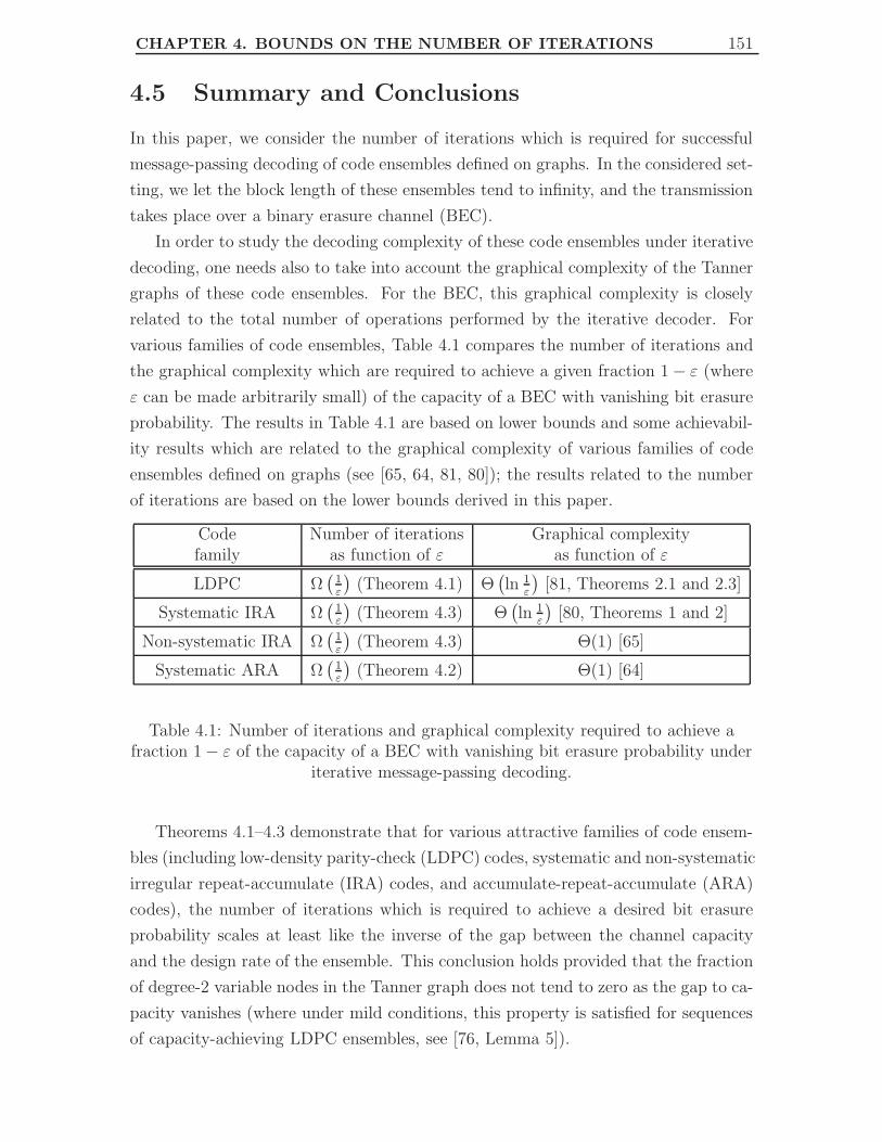
CHAPTER 4. BOUNDS ON THE NUMBER OF ITERATIONS 151
4.5 Summary and Conclusions
In this paper, we consider the number of iterations which is required for successful
message-passing decoding of code ensembles defined on graphs. In the considered set-
ting, we let the block length of these ensembles tend to infinity, and the transmission
takes place over a binary erasure channel (BEC).
In order to study the decoding complexity of these code ensembles under iterative
decoding, one needs also to take into account the graphical complexity of the Tanner
graphs of these code ensembles. For the BEC, this graphical complexity is closely
related to the total number of operations performed by the iterative decoder. For
various families of code ensembles, Table 4.1 compares the number of iterations and
the graphical complexity which are required to achieve a given fraction 1 − ε (where
ε can be made arbitrarily small) of the capacity of a BEC with vanishing bit erasure
probability. The results in Table 4.1 are based on lower bounds and some achievabil-
ity results which are related to the graphical complexity of various families of code
ensembles defined on graphs (see [65, 64, 81, 80]); the results related to the number
of iterations are based on the lower bounds derived in this paper.
Code Number of iterations Graphical complexityfamily as function of ε as function of ε
LDPC Ω(
1ε
)(Theorem 4.1) Θ
(ln 1
ε
)[81, Theorems 2.1 and 2.3]
Systematic IRA Ω(
1ε
)(Theorem 4.3) Θ
(ln 1
ε
)[80, Theorems 1 and 2]
Non-systematic IRA Ω(
1ε
)(Theorem 4.3) Θ(1) [65]
Systematic ARA Ω(
1ε
)(Theorem 4.2) Θ(1) [64]
Table 4.1: Number of iterations and graphical complexity required to achieve afraction 1 − ε of the capacity of a BEC with vanishing bit erasure probability under
iterative message-passing decoding.
Theorems 4.1–4.3 demonstrate that for various attractive families of code ensem-
bles (including low-density parity-check (LDPC) codes, systematic and non-systematic
irregular repeat-accumulate (IRA) codes, and accumulate-repeat-accumulate (ARA)
codes), the number of iterations which is required to achieve a desired bit erasure
probability scales at least like the inverse of the gap between the channel capacity
and the design rate of the ensemble. This conclusion holds provided that the fraction
of degree-2 variable nodes in the Tanner graph does not tend to zero as the gap to ca-
pacity vanishes (where under mild conditions, this property is satisfied for sequences
of capacity-achieving LDPC ensembles, see [76, Lemma 5]).

CHAPTER 4. BOUNDS ON THE NUMBER OF ITERATIONS 152
When the graphical complexity of these families of ensembles is considered, the
results are less homogenous. More explicitly, assume a sequence of LDPC codes (or
ensembles) whose block length tends to infinity, and consider the case where their
transmission takes place over a memoryless binary-input output-symmetric channel.
It follows from [81, Theorem 2.1] that if a fraction 1−ε of the capacity of this channel
is achieved with vanishing bit error (erasure) probability under ML decoding (or any
sub-optimal decoding algorithm), then the graphical complexity of an arbitrary rep-
resentation of the codes using bipartite graphs scales at least like ln 1ε. For systematic
IRA codes which are transmitted over the BEC and decoded by a standard iterative
message-passing decoder, a similar result on their graphical complexity is obtained in
[80, Theorem 1]. In [81, Theorem 2.3], the lower bound on the graphical complexity
of LDPC ensembles is achieved for the BEC (up to a small additive constant), even
under iterative message-passing decoding, by the right-regular LDPC ensembles of
Shokrollahi [94]. Similarly, [80, Theorem 2] presents an achievability result of this
form for ensembles of systematic IRA codes transmitted over the BEC; the graphical
complexity of these ensembles scales logarithmically with 1ε. For ensembles of non-
systematic IRA and systematic ARA codes, however, the addition of state nodes in
their standard representation by Tanner graphs allows to achieve an improved trade-
off between the gap to capacity and the graphical complexity; suitable constructions
of such ensembles enable to approach the capacity of the BEC with vanishing bit
erasure probability under iterative decoding while maintaining a bounded graphical
complexity (see [65] and [64]). We note that the ensembles in [64] have the additional
advantage of being systematic, which allows simple decoding of the information bits.
The lower bounds on the number of iterations in Theorems 4.1–4.3 become trivial
when the fraction of degree-2 variable nodes vanishes. As noted in Discussion 4.2, for
all known capacity-approaching sequences of LDPC ensembles, this fraction tends to 12
as the gap to capacity vanishes. For some ensembles of capacity approaching system-
atic ARA codes presented in [64], the fraction of degree-2 ‘punctured bit’ nodes (as
introduced in Figure 4.1) is defined to be zero (see [64, Table I]). For these ensembles,
the lower bound on the number of iterations in Theorem 4.2 is ineffective. However,
this is mainly a result of our focus on the derivation of simple lower bounds on the
number of iterations which do not depend on the full characterization of the degree
distributions of the code ensembles. Following the proofs of Theorems 4.1 and 4.2,
and focusing on the case where the fraction of degree-2 variable nodes vanishes, it
is possible to derive lower bounds on the number of iterations which are not trivial
even in this case; these bounds, however, require the knowledge of the entire degree
distribution of the examined ensembles.

CHAPTER 4. BOUNDS ON THE NUMBER OF ITERATIONS 153
The simple lower bounds on the number of iterations of graph-based ensembles,
as derived in this paper, scale like the inverse of the gap in rate to capacity and also
depend on the target bit erasure probability. The behavior of these lower bounds
matches well with the experimental results and the conjectures on the number of
iterations and complexity, as provided by Khandekar and McEliece (see [43, 42, 56]).
In [42, Theorem 3.5], it was stated that for LDPC and IRA ensembles which achieve
a fraction 1−ε of the channel capacity of a BEC with a target bit erasure probability
of Pb under iterative message-passing decoding, the number of iterations grows like
O(
1ε
). In light of the outline of the proof of this statement, as suggested in [42, p. 71],
it implicitly assumes that the flatness condition is satisfied for these code ensembles
and also that the target bit erasure probability vanishes; under these assumptions,
the reasoning suggested by Khandekar in [42, Section 3.6] supports the behavior of
the lower bounds which are derived in this paper.
The matching condition for generalized extrinsic information transfer (GEXIT)
curves serves to conjecture in [59, Section XI] that the number of iterations scales
like the inverse of the achievable gap in rate to capacity (see also [57, p. 92]); this
conjecture refers to LDPC ensembles whose transmission takes place over a general
memoryless binary-input output-symmetric (MBIOS) channel. Focusing on the BEC,
the derivation of the lower bounds on the number of iterations (see Section 4.4)
makes the heuristic reasoning of this scaling rigorous. It also extends the bounds to
various graph-based code ensembles (e.g., IRA and ARA ensembles) under iterative
message-passing decoding, and makes them universal for the BEC in the sense that
they are expressed in terms of some basic parameters of the ensembles which include
the fraction of degree-2 variable nodes, the target bit erasure probability and the
asymptotic gap between the channel capacity and the design rate of the ensemble
(but the bounds here do not depend explicitly on the degree distributions of the code
ensembles). An interesting and challenging direction which calls for further research is
to extend these lower bounds on the number of iterations for general MBIOS channels;
as suggested in [59, Section XI], a consequence of the matching condition for GEXIT
curves has the potential to lead to such lower bounds on the number of iterations
which also scale like the inverse of the gap to capacity for general MBIOS channels.
Appendices
4.A Proof of Proposition 4.1
We begin the proof by considering an iterative decoder of systematic ARA codes by
viewing them as interleaved and serially concatenated codes. The outer code of the

CHAPTER 4. BOUNDS ON THE NUMBER OF ITERATIONS 154
systematic ARA code consists of the first accumulator which operates on the system-
atic bits (see the upper zigzag in Figure 4.1), followed by the irregular repetition code.
The inner code consists of the irregular SPC code, followed by the second accumula-
tor (see the lower zigzag in Figure 4.1). These two constituent codes are joined by an
interleaver which permutes the repeated bits at the output of the outer code before
they are used as input to the inner encoder; for the considered ARA ensemble, we
assume that the interleaver is chosen uniformly at random over all interleavers of the
appropriate length. The turbo-like decoding algorithm is based on iterating extrinsic
information between bitwise MAP decoders of the two constituent codes (see e.g.,
[11]). Each decoding iteration begins with an extrinsic bitwise MAP decoding for
each non-systematic output bit of the outer code (these are the bits which serve as
input to the inner code) based on the information regarding these bits received from
the extrinsic bitwise MAP decoder of the inner code in the previous iteration and the
information on the systematic bits received from the communication channel. In the
second stage of the iteration, this information is passed from the outer decoder to an
extrinsic bitwise MAP decoder of the inner code and is used as a-priori knowledge
for decoding the input bits of the inner code. A Tanner graph for turbo-like decod-
ing of systematic ARA codes is presented in Figure 4.3. Considering the asymptotic
case where the block length tends to infinity, we denote the probability of erasure
messages from the outer decoder to the inner decoder and vice versa at the l’th de-
coding iteration by x(l)0 and x
(l)1 , respectively. Keeping in line with the notation in
the proofs of Theorems 4.1 and 4.2, we begin counting the iterations at l = 0. Since
there is no a-priori information regarding the non-systematic output bits of the outer
decoder (which are permuted to form the input bits of the inner decoder, as shown
in Figure 4.3) we have
x(−1)0 = x
(−1)1 = 1. (4.A.1)
We now turn to calculate the erasure probability x(l)0 in an extrinsic bitwise MAP
decoding of non-systematic output bits of the outer code, given that the a-priori
erasure probability of these bits is x(l−1)1 . To this end, we consider the Tanner graph
of the outer code, shown in the top box of Figure 4.3. We note that this Tanner
graph contains no cycles, and therefore bitwise MAP decoding of this code can be
performed by using the standard iterative message-passing decoding algorithm until
a fixed-point is reached. In such a decoder which operates on the Tanner graph of
the outer code, messages are transferred between the ‘punctured bit’ and the ‘parity-
check 1’ nodes of the graph. Let us denote by x0,o(x) the probability of erasure in
messages from the ‘punctured bit’ nodes to the ‘parity-check 1’ nodes at the fixed
point of the iterative decoding algorithm, when the a-priori erasure probability of the

CHAPTER 4. BOUNDS ON THE NUMBER OF ITERATIONS 155
DE
p
x random permutation
outer code
inner code
0 x 1
x 0,ox 1,o
x 1,ix 0,i
paritychecks 1
puncturedbits
paritychecks 2
codebits
bitssystematic
Figure 4.3: Tanner graph of a systematic accumulate-repeat-accumulate (ARA)code for turbo-like decoding as an interleaved and serially concatenated code.
output bits is x. Similarly, we denote by x1,o(x) the erasure probability in messages
from the ’parity-check 1’ nodes to the ’punctured bit’ nodes at the fixed point, where
x is the a-priori erasure probability of the non-systematic output bits. Based on the
structure of the Tanner graph, we have
x0,o(x) = x1,o(x) · L(x) (4.A.2)
and
x1,o(x) = 1 − (1 − p)(1 − x0,o(x)
)(4.A.3)
where L is defined in (4.1) and it forms the degree distribution of the ‘punctured bit’
nodes from the node perspective, and p denotes the erasure probability of the BEC.
Substituting (4.A.2) into (4.A.3) gives
x1,o(x) =p
1 − (1 − p)L(x). (4.A.4)
Therefore, the structure of the Tanner graph of the outer code implies that the erasure
probability x(l)0 in messages from the outer decoder to the inner decoder at iteration
number l of the turbo-like decoding algorithm is given by

CHAPTER 4. BOUNDS ON THE NUMBER OF ITERATIONS 156
x(l)0 =
(x1,o
(x
(l−1)1
))2
λ(x
(l−1)1
)
=
(p
1 − (1 − p)L(x
(l−1)1
))2
λ(x
(l−1)1
)
= λ(x
(l−1)1
)(4.A.5)
where the second equality relies on (4.A.4), and λ is the tilted degree distribution
which results from graph reduction (see (4.29)). We now employ a similar technique
to calculate the erasure probability x(l)1 in an extrinsic bitwise MAP decoding of input
bits of the inner code, given that the a-priori erasure probability of these bits is x(l)0 .
Since the Tanner of the inner code is also cycle-free (see the lower box in Figure 4.3),
extrinsic bitwise MAP decoding can be done by using the iterative decoder operating
on the Tanner graph of the inner code. We denote by x0,i(x) the erasure probability of
messages from the ‘parity check 2’ nodes to the ‘code bit’ nodes at the fixed point of
the iterative decoding algorithm when x is the a-priori erasure probability of the input
bits. Similarly, x1,i(x) designates the erasure probability of messages from the ‘code
bit’ nodes to the ‘parity check 2’ nodes at the fixed point of the decoding algorithm,
when x is the a-priori erasure probability of the input bits. The structure of the
Tanner graph implies that
x0,i(x) = 1 −(1 − x1,i(x)
)R(1 − x) (4.A.6)
andx1,i(x) = p x0,i(x) (4.A.7)
where R is defined in (4.2). Substituting (4.A.6) into (4.A.7) gives
x1,i(x) =p(1 − R(1 − x)
)
1 − p R(1 − x). (4.A.8)
Therefore, the erasure probability x(l)1 in messages from the inner decoder to the outer
decoder at iteration number l of the turbo-like decoding algorithm is given by
x(l)1 = 1 −
(1 − x1,i
(x
(l)0
))2
ρ(1 − x
(l)0
)
= 1 −
1 −
p(1 − R
(1 − x
(l)0
))
1 − p R(1 − x
(l)0
)
2
ρ(1 − x
(l)0
)
= 1 −(
1 − p
1 − p R(1 − x
(l)0
))2
ρ(1 − x
(l)0
)
= 1 − ρ(1 − x
(l)0
)(4.A.9)
CHAPTER 4. BOUNDS ON THE NUMBER OF ITERATIONS 157
where the second equality relies on (4.A.8), and ρ is the tilted degree distribution
resulting from graph reduction (see (4.30)). Combining (4.A.1), (4.A.5) and (4.A.9)
gives
x(0)0 = λ
(x
(−1)1
)= λ(1) = 1 ,
x(l)0 = λ
(1 − ρ
(1 − x
(l−1)0
)), l ∈ N . (4.A.10)
Observing the proof of Theorem 4.2, we note that x(l)0 = x(l) for all l = 0, 1, . . ., where
is the x(l) value at the left tip of the horizontal line hl in Figure 4.2 (see Eq. (4.46)
on page 148).
Let P(l)b designate the average erasure probability of the systematic bits at the end
of the l’th iteration of the turbo-like decoder. From the definition of the turbo-like
decoding algorithm, P(l)b is the erasure probability of bitwise MAP decoding for the
input bits to the outer code, given that the a-priori erasure probability of the output
bits of this code is given by x(l)1 . Based of the structure of the Tanner graph of the
outer code in Figure 4.3, we get
P(l)b = p
[1 −
(1 − x0,o
(x
(l)1
))2]
(4.A.11)
where x0,o(x) in the fixed point erasure probability of messages from the ‘punctured
bit’ nodes to the ‘parity-check 1’ nodes in the case that the a-priori erasure probability
of the non-systematic output bits of the code is x. Substituting (4.A.3) in (4.A.2)
gives
x0,o(x) =p L(x)
1 − (1 − p)L(x).
Substituting the above equality into (4.A.11), we have
P(l)b = p
[1 −
(1 − p L
(x
(l)1
)
1 − (1 − p)L(x
(l)1
))2]
= p
[1 −
(1 − L
(x
(l)1
))2]
= p
[1 −
(1 − L
(1 − ρ
(1 − x
(l)0
)))2]
where the second equality follows from the definition of L in (4.32) and the third
equality relies on (4.A.9). Using simple algebra, the above expression gives
1 −
√
1 − P(l)b
p= L
(1 − ρ
(1 − x
(l)0
)). (4.A.12)

CHAPTER 4. BOUNDS ON THE NUMBER OF ITERATIONS 158
Hence, the lower bound on the average erasure probability of the systematic bits
at the end of the l’th iteration of the standard iterative decoder for ARA codes in
Lemma 4.3 is satisfied (with equality) also for the turbo-like decoder.
Let l designate the required number of iterations for the turbo-like decoder to
achieve an average erasure probability Pb of the systematic bits. Since we start
counting the iterations at zero, (4.A.12) implies that l is the smallest natural number
which satisfies
1 −√
1 − Pb
p≥ L
(1 − ρ
(1 − x
(l−1)0
)).
However, this is exactly the quantity for which we calculated the lower bound in
the proof of Theorem 4.2 (see Lemmas 4.2 and 4.3 and Eq. (4.31)). Therefore, we
conclude that the lower bound on the number of iterations (l) in Theorem 4.2 holds
also when the considered turbo-like decoding algorithm is employed to decode the
systematic ARA codes as interleaved and serially concatenated codes.
4.B Some mathematical details related to the proof
of Theorem 4.2
4.B.1 Proof of Lemma 4.2
The proof of Lemma 4.2 is based on the DE equations in (4.5) for systematic ARA
ensembles. From the DE equations for x(l)2 and x
(l)3 , we have
x(l)3 = p x
(l)2
= p[1 − R
(1 − x
(l)1
)(1 − x
(l−1)3
)]
≥ p[1 − R
(1 − x
(l)1
)(1 − x
(l)3
)]
where the inequality follows since the decoding process does not add erasures, so x(l)i
is monotonically decreasing with l (for i = 0, 1, . . . , 5). This gives
1 − x(l)3 ≤ 1 − p
[1 − R
(1 − x
(l)1
)(1 − x
(l)3
)]
and
1 − x(l)3 ≤ 1 − p
1 − pR(1 − x
(l)1
) . (4.B.1)
CHAPTER 4. BOUNDS ON THE NUMBER OF ITERATIONS 159
Substituting (4.B.1) into the DE equation for x(l)4 (see (4.5)) gives
x(l)4 = 1 −
(1 − x
(l)3
)2
ρ(1 − x
(l)1
)
≥ 1 −
1 − p
1 − pR(1 − x
(l)1
)
2
ρ(1 − x
(l)1
)
= 1 − ρ(1 − x
(l)1
)(4.B.2)
where ρ is defined in (4.30). From (4.5), we get
x(l)5 = x
(l)0 L
(x
(l)4
)
=[1 −
(1 − x
(l−1)5
)(1 − p)
]L(x
(l)4
)
≥[1 −
(1 − x
(l)5
)(1 − p)
]L(x
(l)4
)
where the inequality follows from the monotonicity of x(l)5 . Solving for 1−x
(l)5 gives
1 − x(l)5 ≤
1 − L(x
(l)4
)
1 − (1 − p)L(x
(l)4
) . (4.B.3)
Substituting (4.B.3) into the DE equation for x(l)0 in (4.5), we have
x(l)0 = 1 −
(1 − x
(l−1)5
)(1 − p)
≥ 1 −(1 − p)
[1 − L
(x
(l−1)4
)]
1 − (1 − p)L(x
(l−1)4
)
=p
1 − (1 − p)L(x
(l−1)4
) .
Substituting the inequality above into the DE equation for x(l)1 gives
x(l)1 =
(x
(l)0
)2
λ(x
(l−1)4
)
≥
p
1 − (1 − p)L(x
(l−1)4
)
2
λ(x
(l−1)4
)
= λ(x
(l−1)4
)(4.B.4)
where λ is defined in (4.29). Finally (4.28) follows from (4.B.2) and (4.B.4) and the
monotonicity of λ over the interval [0, 1].

CHAPTER 4. BOUNDS ON THE NUMBER OF ITERATIONS 160
4.B.2 Proof of Lemma 4.3
From the structure of the Tanner graph of systematic ARA codes (see Figure 4.1)
and the DE equation for x(l)5 in (4.5) we get
P(l)b = p
[1 −
(1 − x
(l)5
)2]
= p
[1 −
(1 − x
(l)0 L
(x
(l)4
))2]
. (4.B.5)
The DE equation (4.5) for x(l)1 and (4.29) imply that
(x
(l)0
)2
=x
(l)1
λ(x
(l−1)4
)
=x
(l)1 p2
λ(x
(l−1)4
) [1 − (1 − p) L
(x
(l−1)4
)]2
≥
p
1 − (1 − p) L(x
(l−1)4
)
2
where the last inequality follows from (4.B.4). Taking the square root on both sides
of the above inequality gives
x(l)0 ≥ p
1 − (1 − p) L(x
(l−1)4
) . (4.B.6)
Substituting (4.B.6) in (4.B.5), we get
P(l)b ≥ p
1 −
1 −
p L(x
(l)4
)
1 − (1 − p) L(x
(l−1)4
)
2
≥ p
1 −
1 −p L(x
(l)4
)
1 − (1 − p) L(x
(l)4
)
2 (4.B.7)
where the second inequality above follows since the decoding process does not add
erasures so x(l)4 ≤ x
(l−1)4 , and from the monotonicity of L over [0, 1]. Applying the
definition of L in (4.32) to the RHS of (4.B.7) gives
P(l)b ≥ p
[1 −
(1 − L
(x
(l)4
))2]
≥ p
1 −
[1 − L
(1 − ρ
(x
(l)1
))]2(4.B.8)
where the last inequality follows from (4.B.2). Finally, (4.34) follows directly from
(4.B.8).

Chapter 5
An Improved Sphere-Packing
Bound for Finite-Length Codes
over Symmetric Memoryless
Channels
This chapter is a preprint of
• G. Wiechman and I. Sason, “An improved sphere-packing bound for finite-
length codes on symmetric memoryless channels,” submitted to IEEE Trans.
on Information Theory, March 2007.
Chapter Overview: This paper derives an improved sphere-packing (ISP) bound for
finite-length error-correcting codes whose transmission takes place over symmetric
memoryless channels, and the codes are decoded with an arbitrary list decoder. We
first review classical results, i.e., the 1959 sphere-packing (SP59) bound of Shannon
for the Gaussian channel, and the 1967 sphere-packing (SP67) bound of Shannon
et al. for discrete memoryless channels. An improvement on the SP67 bound, as
suggested by Valembois and Fossorier, is also discussed. These concepts are used for
the derivation of a new lower bound on the error probability of list decoding (referred
to as the ISP bound) which is uniformly tighter than the SP67 bound and its improved
version. The ISP bound is applicable to symmetric memoryless channels, and some
of its applications are exemplified. Its tightness under ML decoding is studied by
comparing the ISP bound to previously reported upper and lower bounds on the ML
decoding error probability, and also to computer simulations of iteratively decoded
turbo-like codes. This paper also presents a technique which performs the entire
calculation of the SP59 bound in the logarithmic domain, thus facilitating the exact
calculation of this bound for moderate to large block lengths without the need for the
asymptotic approximations provided by Shannon.
161

CHAPTER 5. AN IMPROVED SPHERE-PACKING BOUND 162
5.1 Introduction
The theoretical study of the fundamental performance limitations of long block codes
was initiated by Shannon. During the fifties and sixties, this research work attracted
Shannon and his colleagues at MIT and Bell Labs (see, e.g., the collected papers of
Shannon [96] and the book of Gallager [32]). An overview of these classical results
and their impact was addressed by Berlekamp [13].
The 1959 sphere-packing (SP59) bound of Shannon [89] serves for the evaluation of
the performance limits of block codes whose transmission takes place over an AWGN
channel. This lower bound on the decoding error probability is expressed in terms
of the block length and rate of the code; however, it does not take into account the
modulation used, but only assumes that the signals are of equal energy. It is often
used as a reference for quantifying the sub-optimality of error-correcting codes under
some practical decoding algorithms.
The 1967 sphere-packing (SP67) bound, derived by Shannon, Gallager and Berlekamp
[87], provides a lower bound on the decoding error probability of block codes as a func-
tion of their block length and code rate, and applies to arbitrary discrete memoryless
channels. Like the random-coding bound (RCB) of Gallager [31], the SP67 bound
decays to zero exponentially with the block length for all rates below the channel
capacity. Further, the error exponent of the SP67 bound is known to be tight at the
portion of the rate region between the critical rate (Rc) and the channel capacity;
for all the rates in this range, the error exponents of the SP67 bound and the RCB
coincide (see [87, Part 1]).
The introduction of turbo-like codes, which closely approach the Shannon capacity
limit with moderate block lengths and a feasible decoding complexity, stirred up new
interest in studying the limits of code performance as a function of the block length
(see, e.g., [27, 44, 45, 55, 79, 98, 109, 115]). In a recent paper [20], Costello and Forney
survey the evolution of channel coding techniques, and also address the significant
contributions of error-correcting codes in improving the tradeoff between performance,
block length (delay) and complexity for practical applications.
In spite of the exponential decay of the SP67 bound in terms of the block length at
all rates below the channel capacity, this bound appears to be loose for codes of small
to moderate block lengths. The weakness of this bound is due to the original focus
in [87] on asymptotic analysis. In [109], Valembois and Fossorier revisited the SP67
bound in order to improve its tightness for finite-length block codes (especially, for
codes of short to moderate block lengths), and also extended its validity to memoryless
continuous-output channels (e.g., the binary-input AWGN channel). The remarkable
CHAPTER 5. AN IMPROVED SPHERE-PACKING BOUND 163
improvement of their bound over the classical SP67 bound was exemplified in [109].
Moreover, the extension of the bound in [109] to memoryless continuous-output chan-
nels provides an alternative to the SP59 bound which holds for the AWGN channel
[89].
This paper is focused on the study of the fundamental performance limitations
of finite-length error-correcting codes and the tradeoff between their performance
and block length when the transmission takes place over an arbitrary symmetric
memoryless channel. This study is facilitated by theoretical bounds, and it is also
compared to the performance of modern coding techniques under sub-optimal and
practical decoding algorithms. In this work, we derive an improved sphere-packing
bound (referred to as the ‘ISP bound’) which improves the bounding techniques in
[87] and [109], especially for codes of short to moderate block lengths; this new bound
is valid for all symmetric memoryless channels.
The structure of this paper is as follows: Section 5.2 reviews the concepts used in
the derivation of the SP67 bound [87, Part 1] and its improved version in [109]. In
Section 5.3, we derive the ISP bound which improves the bound in [109] for symmetric
memoryless channels where the derivation of the ISP bound relies on concepts and
notation presented in Section 5.2. Section 5.4 starts by reviewing the SP59 bound
of Shannon [89], and presenting an algorithm used in [109] for a numerical calcula-
tion this bound. The numerical instability of this algorithm for codes of moderate
to large block lengths motivates the derivation of an alternative algorithm in Sec-
tion 5.4 which facilitates the exact calculation of the SP59 bound, irrespectively of
the block length. Section 5.5 provides numerical results which serve to compare the
ISP bound to previously reported sphere-packing bounds. The tightness of the ISP
bound is exemplified in Section 5.5 for various communication channels. Additionally,
sphere-packing bounds are applied in Section 5.5 to study the tradeoff between the
performance and the required block length of error-correcting codes. We conclude
our discussion in Section 5.6. Some technical details are relegated to the appendices.
5.2 The 1967 Sphere-Packing Bound and Improve-
ments
In the following, we present the SP67 bound and its improvement in [109], followed
by an outline of their derivation. Classical sphere-packing bounds are reviewed in
[79, Chapter 5]. This section serves as a preparatory step towards the derivation of
an improved sphere-packing bound in the next section.
CHAPTER 5. AN IMPROVED SPHERE-PACKING BOUND 164
5.2.1 The 1967 Sphere-Packing Bound
Let us consider a block code C which consists of M codewords each of length N , and
denote its codewords by x1, . . . ,xM. Assume that C is transmitted over a discrete
memoryless channel (DMC) and is decoded by a list decoder; for each received se-
quence y, the decoder outputs a list of at most L integers from the set 1, 2, . . . , Mwhich correspond to the indices of the codewords. A list decoding error is declared if
the index of the transmitted codeword does not appear in the list. Originally intro-
duced by Elias [29] and Wozencraft [120], list decoding signifies an important class
of decoding algorithms. During the last decade, there has been a significant break-
through in the construction of efficient list-decoding algorithms for error-correcting
codes (see, e.g., [33], [75, Chapter 9] and references therein).
A lower bound on the decoding error probability of an arbitrary block code with
M codewords of length N is derived in [87]. This bound applies to an arbitrary list
decoder where the size of the list is limited to L. The particular case where L = 1
clearly provides a lower bound on the error probability under maximum-likelihood
(ML) decoding.
Let Ym designate the set of output sequences y for which message m is on the
decoding list, and define Pm(y) , Pr(y|xm). The conditional error probability under
list decoding when message m is sent over the channel is given by
Pe,m =∑
y∈Ycm
Pm(y) (5.1)
where the superscript ‘c’ stands for the complementary set. For the block code
and list decoder under consideration, let Pe,max designate the maximal value of Pe,m
where m ∈ 1, 2, . . . , M. Assuming that all the codewords are equally likely to be
transmitted, the average decoding error probability is given by
Pe =1
M
M∑
m=1
Pe,m.
Referring to a list decoder of size at most L, the code rate is defined as R ,ln(M
L )N
nats per channel use.
The derivation of the SP67 bound [87, Part 1] is divided into three main steps. The
first step refers to the derivation of upper and lower bounds on the error probability
of a code consisting of two codewords only. These bounds are given by the following
theorem:

CHAPTER 5. AN IMPROVED SPHERE-PACKING BOUND 165
Theorem 5.1 [Upper and Lower Bounds on the Pairwise Error Probability]
[87, Theorem 5]. Let P1 and P2 be two probability assignments defined over a discrete
set of sequences Y , Y1 and Y2 = Yc1 be (disjoint) decision regions for these sequences,
Pe,1 and Pe,2 be given by (5.1), and assume that P1(y)P2(y) 6= 0 for at least one
sequence y. Then, for all s ∈ (0, 1)
Pe,1 >1
4exp(µ(s) − sµ′(s) − s
√2µ′′(s)
)(5.2)
or
Pe,2 >1
4exp(µ(s) + (1 − s)µ′(s) − (1 − s)
√2µ′′(s)
)(5.3)
where
µ(s) , ln(∑
y
P1(y)1−sP2(y)s), 0 < s < 1. (5.4)
Furthermore, for an appropriate choice of the decision regions Y1 and Y2, the following
upper bounds hold:
Pe,1 ≤ exp(µ(s) − sµ′(s)
)(5.5)
and
Pe,2 ≤ exp(µ(s) + (1 − s)µ′(s)
). (5.6)
The function µ is non-positive and convex over the interval (0, 1). The convexity of
µ is strict unless P1(y)P2(y)
is constant over all the sequences y for which P1(y)P2(y) 6= 0.
Moreover, the function µ is strictly negative over the interval (0, 1) unless P1(y) =
P2(y) for all y.
In the following, we present an outline of the proof of Theorem 5.1 which serves
to emphasize the parallelism between Theorem 5.1 and the first part of the derivation
of the ISP bound in Section 5.3. A detailed proof of this theorem is given in [87,
Section III].
Proof: Let us define the log-likelihood ratio (LLR) as
D(y) , ln
(P2(y)
P1(y)
)(5.7)
and the probability distribution
Qs(y) ,P1(y)1−sP2(y)s
∑y′ P1(y′)1−sP2(y′)s
, 0 < s < 1. (5.8)
It is simple to show that for all 0 < s < 1, the first and second derivatives of µ in
(5.4) are equal to the statistical expectation and variance of the LLR, respectively,

CHAPTER 5. AN IMPROVED SPHERE-PACKING BOUND 166
taken with respect to (w.r.t.) the probability distribution Qs in (5.8). This gives the
following equalities:
µ′(s) = EQs
(D(y)
)(5.9)
µ′′(s) = VarQs
(D(y)
). (5.10)
Also, as can be readily verified from (5.4), (5.7) and (5.8)
P1(y) = exp(µ(s) − sD(y)
)Qs(y) (5.11)
P2(y) = exp(µ(s) + (1 − s)D(y)
)Qs(y). (5.12)
For 0 < s < 1, the equalities in (5.9) and (5.10) motivate the definition of a set of
typical sequences w.r.t. the probability distribution Qs as followed:
Ys ,
y ∈ Y : |D(y) − µ′(s)| ≤
√2µ′′(s)
. (5.13)
For any choice of a decision region Y1, the conditional error probability given that
the first message was transmitted satisfies
Pe,1 =∑
y∈Yc1
P1(y)
≥∑
y∈Yc1
TYs
P1(y)
(a)=
∑
y∈Yc1
TYs
exp(µ(s) − sD(y)
)Qs(y)
(b)
≥ exp(µ(s) − sµ′(s) − s
√2µ′′(s)
) ∑
y∈Yc1
TYs
Qs(y) (5.14)
where (a) follows from (5.11) and (b) relies on the definition of Ys in (5.13). Using
similar arguments and relying on (5.12), we also get that
Pe,2 ≥ exp(µ(s) + (1 − s)µ′(s) − (1 − s)
√2µ′′(s)
) ∑
y∈Yc2
TYs
Qs(y) . (5.15)
Since Y1 and Y2 form a partition of the observation space, we have that
∑
y∈Yc1
TYs
Qs(y) +∑
y∈Yc2
TYs
Qs(y) =∑
y∈Ys
Qs(y) >1
2
where the last transition relies on (5.9), (5.10) and (5.13), and it follows from Cheby-
chev’s inequality. Therefore, at least one of the two sums on the LHS of the expression
above must be greater than 14. Substituting this in (5.14) and (5.15) completes the

CHAPTER 5. AN IMPROVED SPHERE-PACKING BOUND 167
proof on the satisfiability of at least one of the inequalities (5.2) and (5.3). The upper
bound on the error probability in (5.5) and (5.6) is attained by selecting the decision
region for the first codeword to be
Y1 ,y ∈ Y : D(y) < µ′(s)
and the decision region for the second code as Y2 , Yc1. The proof for the upper
bounds in (5.5) and (5.6) follows directly from (5.11), (5.12) and the particular choice
of Y1 and Y2 as above.
The initial motivation of Theorem 5.1 is the calculation of lower bounds on the
error probability of a two-word code. Note that this theorem is valid for any pair
of probability assignments P1 and P2 and decision regions Y1 and Y2 which form a
partition of the observation space.
In the continuation of the derivation of the SP67 bound in [87], this theorem is
used in order to control the size of a decision region of a particular codeword without
directly referring to the other codewords. To this end, an arbitrary probability tilting
measure fN is introduced in [87] over all N -length sequences of channel outputs,
requiring that it is factorized in the form
fN(y) =
N∏
n=1
f(yn) (5.16)
for an arbitrary output sequence y = (y1, . . . , yN). The size of the set Ym is defined
as
F (Ym) ,∑
y∈Ym
fN (y). (5.17)
Next, [87] relies on Theorem 5.1 in order to relate the conditional error probability
Pe,m and F (Ym) for fixed composition codes; this is done by associating Pr(·|xm) and
fN with P1 and P2, respectively. Theorem 5.1 is applied to derive a parametric lower
bound on the size of the decision region Ym or on the conditional error probability
Pe,m. Due to the fact that the list size is limited to L, then
M∑
m=1
F (Ym) =
M∑
m=1
∑
y∈Ym
fN(y) ≤ L
since for every sequence y, the relation y ∈ Ym holds for at most L indices m ∈1, . . . , M, and
∑y fN(y) = 1. Therefore, there exists an index m so that F (Ym) ≤
LM
and for this unknown value of m, one can upper bound the conditional error
probability Pe,m by
Pe,max , maxm∈1,...,M
Pe,m.

CHAPTER 5. AN IMPROVED SPHERE-PACKING BOUND 168
Using Theorem 5.1 with the above setting for the probability assignments P1 and P2,
then Pe,1 and Pe,2 on the LHS of (5.2) and (5.3) are respectively replaced by Pe,m and
F (Ym). For the above unknown value of m, whose existence is assured to be in the
set 1, . . . , M, one can replace Pe,m and F (Ym) on the LHS of (5.2) and (5.3) by
their upper bounds Pe,max and LM
, respectively. This provides a lower bound on Pe,max
as long as the inequality which follows from the replacement of F (Ym) by its upper
bound(
LM
)on the LHS of (5.3) does not hold. Next, the probability assignment
f , fs is optimized in [87], so as to get the tightest (i.e., maximal) lower bound
on Pe,max within this form while considering a code whose composition minimizes
the bound (so that the bound holds for all fixed composition codes). A solution for
this min-max problem, as provided in [87, Eqs. (4.18)–(4.20)], leads to the following
theorem which gives a lower bound on the maximal decoding error probability of an
arbitrary fixed composition block code (for a more detailed review of these concepts,
see [79, Section 5.3]).
Theorem 5.2 [Sphere-Packing Bound on the Maximal Error Probability of
Fixed Composition Codes] [87, Theorem 6]. Let C be a fixed composition block
code of M codewords and length N . Assume that the transmission of C takes place
over a DMC, and let P (j|k) be the set of transition probabilities characterizing this
channel (where j ∈ 0, . . . , J − 1 and k ∈ 0, . . . , K − 1 designate the channel
output and input, respectively). For an arbitrary list decoder where the size of the
list is limited to L, the maximal error probability (Pe,max) satisfies
Pe,max ≥ exp
[−N
(Esp
(R − ln 4
N− ε)
+
√8
Nln( e√
Pmin
)+
ln 4
N
)]
where R ,ln(
ML
)
Nis the rate of the code, Pmin designates the smallest non-zero
transition probability of the DMC, the parameter ε is an arbitrarily small positive
number, and the function Esp is given by
Esp(R) , supρ≥0
(E0(ρ) − ρR
)(5.18)
E0(ρ) , maxq
E0(ρ,q) (5.19)
E0(ρ,q) , − ln
(J−1∑
j=0
[K−1∑
k=0
qkP (j|k)1
1+ρ
]1+ρ
). (5.20)
The maximum in the RHS of (5.19) is taken over all probability vectors q = (q0, . . . , qK−1),
i.e., over all q with K non-negative components summing to 1.
CHAPTER 5. AN IMPROVED SPHERE-PACKING BOUND 169
The reason for considering fixed composition codes in [87] is that, in general, the
optimal probability distribution fs may depend on the composition of the codewords
through the choice of the parameter s in (0, 1) (see [87, p. 96]).
The next step in the derivation of the SP67 bound is the application of Theo-
rem 5.2 to obtain a lower bound on the maximal decoding error probability of an
arbitrary block code. This is performed by lower bounding the maximal decoding
error probability of a block code by the maximal error probability of its largest fixed
composition subcode. Since the number of possible compositions is polynomial in the
block length, one can lower bound the rate of the largest fixed composition subcode
by R−O(
ln NN
)where R is the rate of the original code. Clearly, the rate loss caused
by considering this subcode vanishes when the block length tends to infinity; however,
it loosens the bound for codes of short to moderate block lengths. Finally, the bound
on the maximal block error probability is transformed into a bound on the average
block error probability by considering an expurgated code which contains half of the
codewords of the original code with the lowest conditional error probability. This
finally leads to the SP67 bound in [87, Part 1].
Theorem 5.3 [The 1967 Sphere-Packing Bound for Discrete Memoryless
Channels] [87, Theorem 2]. Let C be an arbitrary block code whose transmission
takes place over a DMC. Assume that the DMC is specified by the set of transition
probabilities P (j|k) where k ∈ 0, . . . , K − 1 and j ∈ 0, . . . , J − 1 designate the
channel input and output alphabets, respectively. Assume that the code C forms a
set of M codewords of length N (i.e., each codeword is a sequence of N letters from
the input alphabet), and consider an arbitrary list decoder where the size of the list
is limited to L. Then, the average decoding error probability of the code C satisfies
Pe(N, M, L) ≥ exp
−N
[Esp
(R − O1
( ln N
N
))+ O2
( 1√N
)]
where R ,ln(
ML
)
N, and the error exponent Esp(R) is introduced in (5.18). The terms
O1
( ln N
N
)=
ln 8
N+
K ln N
N(5.21)
O2
( 1√N
)=
√8
Nln( e√
Pmin
)+
ln 8
N
scale like lnNN
and 1√N
, respectively (hence, they both vanish as we let N tend to
infinity), and Pmin denotes the smallest non-zero transition probability of the DMC.

CHAPTER 5. AN IMPROVED SPHERE-PACKING BOUND 170
5.2.2 Recent Improvements on the 1967 Sphere-Packing Bound
In [109], Valembois and Fossorier revisited the derivation of the SP67 bound, focus-
ing on finite-length block codes. They presented four modifications to the classical
derivation in [87] which improve the pre-exponent of the SP67 bound. The new
bound derived in [109] is also valid for memoryless channels with discrete input and
continuous output (as opposed to the SP67 bound which is only valid for DMCs). In
this section, we outline the improvements suggested in [109] and present the resulting
bound.
The first modification suggested in [109] is the addition of a free parameter in the
derivation of the lower bound on the decoding error probability of two-word codes; this
free parameter is used in conjunction with Chebychev’s inequality, and it is optimized
in order to tighten the lower bounds on Pe,1 and Pe,2 in Theorem 5.1 (see (5.2), (5.3)).
A second improvement presented in [109] is related to the inequality s√
µ′′(s) ≤ln(
e√Pmin
)which was applied to simplify the final form of the bound in Theorem 5.3
(see [87, Part 1]). This bound on the second derivative of µ results in no asymptotic
loss, but it loosens the lower bound on the decoding error probability for finite-length
codes (especially, for short to moderate block lengths). By using the exact value of
µ′′ instead, the tightness of the resulting bound is further improved in [109]. This
modification also makes the bound suitable to memoryless channels with a continuous
output alphabet, as it is no longer required that Pmin is positive. It should be noted
that this causes a small discrepancy in the derivation of the bound; the derivation of a
lower bound on the block error probability which is uniform over all fixed composition
codes relies on finding the composition which minimizes the lower bound. The optimal
composition is given in [87, Eqs. (4.18), (4.19)] for the case where the upper bound
on µ′′ is applied. In [109], the same composition is used without checking whether
it is still the composition which minimizes the lower bound. However (as we see in
the next section), for the class of symmetric memoryless channels, the value of the
bound is independent of the code composition; therefore, the bound of Valembois and
Fossorier [109, Theorem 7] (referred to as the ‘VF bound’) stays valid. This class of
channels includes all memoryless binary-input output-symmetric (MBIOS) channels.
A third improvement in [109] refers to the particular selection of the value of
ρ ≥ 0 which leads to the derivation of Theorem 5.3. In [87], ρ is set to be the value ρ
which maximizes the error exponent of the SP67 bound (i.e., the upper bound on the
error exponent). This choice emphasizes the similarity between the error exponents
of the SP67 bound and the RCB, hence proving that the error exponent of the SP67
bound is tight for all rates above the critical rate of the channel. In order to tighten
the bound for finite-length block codes, [109] chooses the value of ρ to be ρ∗ which

CHAPTER 5. AN IMPROVED SPHERE-PACKING BOUND 171
provides the tightest possible lower bound on the decoding error probability. For
rates above the critical rate of the channel, the tightness of the error exponent of the
classical SP67 bound implies that ρ tends to ρ∗ as the block length tends to infinity.
However, for codes of finite block length, this simple observation tightens the bound
with almost no penalty in the computational complexity of the resulting bound.
The fourth observation made in [109] refers to the final stage in the derivation
of the SP67 bound. In order to get a lower bound on the maximal decoding error
probability of an arbitrary block code, the derivation in [87] considers the maximal
decoding error probability of a fixed composition subcode of the original code. In [87],
a simple lower bound on the size of the largest fixed composition subcode is given;
namely, the size of the largest fixed composition subcode is not less than the size of
the entire code divided by the number of possible compositions. Since the number of
possible compositions is equal to the number of possible ways to divide N symbols
into K types, this value is given by(
N+K−1K−1
). To simplify the final expression of the
SP67 bound, [87] relies on the inequality(
N+K−1K−1
)≤ NK which provides a simple
upper bound on the number of compositions. Since this expression is polynomial
is the block length N , there is no asymptotic loss to the error exponent. However,
by using the exact expression for the number of possible compositions, the bound in
[109] is tightened for codes of short to moderate block lengths. Applying these four
modifications in [109] to the derivation of the SP67 bound yields an improved lower
bound on the decoding error probability of block codes transmitted over memoryless
channels with finite input alphabets. As mentioned above, these modifications also
extend the validity of the new bound to memoryless channels with discrete input and
continuous output. However, the requirement of a finite input alphabet still remains,
as it is required to apply the bound to arbitrary block codes, and not only to fixed
composition codes. Under the assumptions and notation used in Theorem 5.3, the
VF bound [109] is given in the following theorem:
Theorem 5.4 [Improvement on the 1967 Sphere-Packing Bound for Dis-
crete Memoryless Channels] [109, Theorem 7]. The average decoding error prob-
ability satisfies Pe(N, M, L) ≥ exp(−NEVF(R, N)
)where
EVF(R, N) ,
∫
x>√
22
E0(ρx) − ρx
(R − O1
( ln N
N, x))
+ O2
( 1√N
, x, ρx
)
and
O1
( ln N
N, x)
,ln 8
N+
ln(
N+K−1K−1
)
N− ln
(2 − 1
x2
)
N(5.22)

CHAPTER 5. AN IMPROVED SPHERE-PACKING BOUND 172
O2
( 1√N
, x, ρ)
, x
√√√√ 8
N
K−1∑
k=0
qk,ρν(2)k (ρ) +
ln 8
N− ln
(2 − 1
x2
)
N
ν(1)k (ρ) ,
J−1∑
j=0
βj,k,ρ lnβj,k,ρ
P (j|k)
J−1∑
j=0
βj,k,ρ
ν(2)k (ρ) ,
J−1∑
j=0
βj,k,ρ ln2 βj,k,ρ
P (j|k)
J−1∑
j=0
βj,k,ρ
−[ν
(1)k (ρ)
]2
βj,k,ρ , P (j|k)1
1+ρ ·(
K−1∑
k′=0
qk′,ρP (j|k′)1
1+ρ
)ρ
where qρ , (q1,ρ, . . . , qK,ρ) designates the input distribution which maximizes E0(ρ,q)
in (5.19), and the parameter ρ = ρx is determined by solving the equation
R − O1
( ln N
N, x)
= −1
ρ
K−1∑
k=0
qk,ρν(1)k (ρ) +
x
ρ
√√√√ 2
N
K−1∑
k=0
qk,ρν(2)k (ρ).
For a more detailed review of the improvements suggested in [109], the reader is
referred to [79, Section 5.4].
Remark 5.1 The rate loss as a result of the expurgation of the code by removing half
of the codewords with the largest error probability was ignored in [109]. The termln 4N
, as it appears in the term O1(ln NN
, x) of [109, Theorem 7], should be therefore
replaced by ln 8N
(see (5.22)).
5.3 An Improved Sphere-Packing Bound for Sym-
metric Memoryless Channels
In this section, we derive an improved lower bound on the decoding error probability
which utilizes the sphere-packing bounding technique. This new bound is valid for
symmetric memoryless channels with a finite input alphabet, and is referred to as
an improved sphere-packing (ISP) bound. Note that the symmetry of the channel is
crucial for the derivation of the ISP bound in this section, which stays in contrast to
the SP67 and VF bounds where channel symmetry is not required. We begin with

CHAPTER 5. AN IMPROVED SPHERE-PACKING BOUND 173
some necessary definitions and basic properties of symmetric memoryless channels
which are used in this section for the derivation of the ISP bound.
5.3.1 Symmetric Memoryless Channels
Definition 5.1 A bijective mapping g : J → J where J ⊆ Rd is said to be unitary
if for any integrable generalized function f : J → R
∫
Jf(x)dx =
∫
Jf(g(x))dx (5.23)
where by generalized function we mean a function which may contain a countable
number of shifted Dirac delta functions. If the projection of J over some of the d
dimensions is countable, the integration over these dimensions is turned into a sum.
Remark 5.2 The following properties also hold:
1. If g is a unitary mapping so is its inverse g−1.
2. If J is a countable set, then g : J → J is unitary if and only if g is bijective.
3. Let J be an open set and g : J → J be a bijective function. Denote
g(x1, . . . , xd) ,(g1(x1, . . . , xd), . . . , gd(x1, . . . , xd)
)
and assume that the partial derivatives ∂gi
∂xjexist for all i, j ∈ 1, 2, . . . , d. Then
g is unitary if and only if the Jacobian satisfies |J(x)| = 1 for all x ∈ J .
Proof: The first property follows from (5.23) and by defining f(x) , f(g−1(x)
); this
gives∫
Jf(g−1(x)
)dx =
∫
Jf(x)dx =
∫
Jf(g(x)
)dx =
∫
Jf((g−1 g)(x)
)dx =
∫
Jf(x)dx .
The second property follows from the fact that for countable sets, the integral is
turned into a sum, and the equality
∑
j∈Jf(j) =
∑
j∈Jf(g(j)
)
holds by changing the order of summation. Finally, the third property is proved by
a transform of the integrator on the LHS of (5.23) from x = (x1, . . . , xd) to g(x).
We are now ready to define K-ary input symmetric channels. The symmetry
properties of these channels are later exploited to improve the tightness of the sphere-
packing bounding technique and derive the ISP lower bound on the average decoding
error probability of block codes transmitted over these channels.

CHAPTER 5. AN IMPROVED SPHERE-PACKING BOUND 174
Definition 5.2 [Symmetric Memoryless Channels] A memoryless channel with
input alphabet K = 0, 1, . . . , K − 1, output alphabet J ⊆ Rd (where K, d ∈ N)
and transition probability (or density if J non-countable) function P (·|·) is said to
be symmetric if there exists a set of bijective and unitary mappings gkK−1k=0 where
gk : J → J for all k ∈ K such that
∀y ∈ J , k ∈ K P (y|0) = P(gk(y)|k
)(5.24)
and
∀k1, k2 ∈ K g−1k1
gk2 = g(k2−k1)modK . (5.25)
Remark 5.3 From (5.24), the mapping g0 is the identity mapping. Assigning k1 = k
and k2 = 0 in (5.25) gives
∀k ∈ K g−1k = g(−k)modK = gK−k . (5.26)
The class of symmetric memoryless channels, as given in Definition 5.2, is quite
large. In particular, it contains the class of memoryless binary-input output-symmetric
(MBIOS) channels. To show this, we employ the following proposition which follows
from the discussion in [74, Section 4.1.4]:
Proposition 5.1 An MBIOS channel can be equivalently represented as a (time-
varying) binary symmetric channel (BSC) whose crossover probability for each output
symbol is an i.i.d. random variable which is independent of the channel input, and
observed by the receiver. This crossover probability is given by p = 11+exp(|L|) where
L = L(y) denotes the log-likelihood ratio which corresponds to the channel output y.
We now apply Proposition 5.1 to show that any MBIOS channel is a symmetric
memoryless channel, according to Definition 5.2.
Corollary 5.1 An arbitrary MBIOS channel, can be equivalently represented as a
symmetric memoryless channel.
Proof: Let us consider an MBIOS channel C. Applying Proposition 5.1, it can be
equivalently represented by a channel C′ whose output alphabet is J = 0, 1× [0, 1];
here, the first term of the output refers to the BSC output and the second term is
the associated crossover probability. We now show that this equivalent channel is a
symmetric memoryless channel. To this end, it suffices to find a unitary mapping
g1 : J → J such that∀y ∈ J P (y|0) = P
(g1(y)|1
)(5.27)
and g−11 = g1 (i.e., g1 is equal to its inverse).

CHAPTER 5. AN IMPROVED SPHERE-PACKING BOUND 175
For the channel C′, the conditional probability distribution (or density) function
of the output y = (m, p) (where m ∈ 0, 1 and p ∈ [0, 1]) given that i ∈ 0, 1 is
transmitted, is given by
P (y|i) =
P (p) · (1 − p) if i = m
P (p) · p if i = m(5.28)
where P is a distribution (or density) over [0, 1] and m designates the logical not of m.
From (5.28), we get that the mapping g1(m, p) =(m, p
)satisfies (5.27). Additionally,
g−11 = g1 since m = m. Therefore, the proof is completed by showing that g1 is a
unitary mapping. For any (generalized) function f : J → R we have
∫
Jf(x)dx ,
1∑
m=0
∫ 1
0
f(m, p)dp
=
1∑
m=0
∫ 1
0
f(m, p)dp
=
∫
Jf(g1(x)
)dx
where the second equality holds by changing the order of summation; hence g1 is a
unitary function.
Remark 5.4 Proposition 5.1 forms a special case of a proposition given in [113,
Appendix I]. Using the proposition in [113, Appendix I], which refers to M-ary input
channels, it can be shown in a similar way that all M-ary input symmetric output
channels, as defined in [113], can be equivalently represented as symmetric memoryless
channels.
Coherently detected M-ary PSK modulated signals transmitted over a fully inter-
leaved fading channel, followed by an additive white Gaussian noise, form another
example of a symmetric memoryless channel. In this case, J = R2 and the mapping
gk for k = 0, . . . , M − 1 forms a clockwise rotation by 2πkM
(i.e., gk(y) = exp(
2jπk
M
)y).
Note that the determinant of the Jacobian of these rotation mappings is equal in
absolute value to 1.
5.3.2 Derivation of an Improved Sphere-Packing Bound for
Symmetric Memoryless Channels
In this section, we derive an improved sphere-packing lower bound on the decoding
error probability of block codes transmitted over symmetric memoryless channels.

CHAPTER 5. AN IMPROVED SPHERE-PACKING BOUND 176
To keep the notation simple, we derive the bound under the assumption that the
communication takes place over a symmetric DMC. However, the derivation of the
bound is justified later for the general class of symmetric memoryless channels with
discrete or continuous output alphabets. Some remarks are given at the end of the
derivation.
Though there is a certain parallelism to the derivation of the SP67 bound in
[87, Part 1], our analysis for symmetric memoryless channels deviates considerably
from the derivation of this classical bound. The improvements suggested in [109]
are also incorporated into the derivation of the bound. We show that for symmetric
memoryless channels, the derivation of the sphere-packing bound can be modified
so that the intermediate step of bounding the maximal error probability for fixed
composition codes can be skipped, and one can directly consider the average error
probability of an arbitrary block code. To this end, the first step of the derivation
in [87] (see Theorem 5.1 here) is modified so that instead of bounding the error
probability when a single pair of probability assignments is considered, we consider
the average error probability over M pairs of probability assignments.
Average Decoding Error Probability for M Pairs of Probability Assign-
ments
We start the analysis by considering the average decoding error probability over M
pairs of probability assignments, denoted P m1 , P m
2 Mm=1, where it is assumed that the
index m of the pair is chosen uniformly at random from the set 1, . . . , M and is
known to the decoder. Denote the observation by y and the observation space by Y .
For simplicity, we assume that Y is a finite set. Following the notation in [87], we
define the LLR for the mth pair of probability assignments as
Dm(y) , ln
(P m
2 (y)
P m1 (y)
)(5.29)
and the probability distribution
Qms (y) ,
P m1 (y)1−s P m
2 (y)s
∑y′ P m
1 (y′)1−s P m2 (y′)s
, 0 ≤ s ≤ 1 . (5.30)
For the mth pair, we also define the function µm as
µm(s) , ln
(∑
y
P m1 (y)1−s P m
2 (y)s
), 0 ≤ s ≤ 1 . (5.31)
Let us assume that µm and its first and second derivatives w.r.t. s are independent
of the value of m, and therefore we can define µ , µ1 = µ2 = . . . = µM .

CHAPTER 5. AN IMPROVED SPHERE-PACKING BOUND 177
Remark 5.5 Note that in this setting, the requirement that µm is independent of m
inherently yields that all its derivatives are also independent of m. However, in the
continuation, we will let P m2 be a function of s and differentiate µm w.r.t. s while
holding P m2 fixed. In this setting, we will show that for the specific selection of P m
1
and P m2 which are used to derive the new lower bound on the average block error
probability, if the communication takes place over a symmetric memoryless channel
then µm and its first two derivatives w.r.t. s are independent of m. Also note that
the fact that µm is independent of m does not imply that P mk is independent of m.
Based on the assumption above, it can be easily verified (in parallel to (5.9)–(5.12))
that for all m ∈ 1, . . . , M
µ′(s) =(µm)′
(s) = EQms
(Dm(y)
)(5.32)
µ′′(s) =(µm)′′
(s) = VarQms
(Dm(y)
)(5.33)
P m1 (y) = exp
(µ(s) − sDm(y)
)Qm
s (y) (5.34)
P m2 (y) = exp
(µ(s) + (1 − s)Dm(y)
)Qm
s (y) (5.35)
where EQ and VarQ stand, respectively, for the statistical expectation and variance
w.r.t. a probability distribution Q. For the mth code book, we define the set of typical
output vectors as
Ym,xs ,
y ∈ Y : |Dm(y) − µ′(s)| ≤ x
√2µ′′(s)
, x > 0. (5.36)
In the original derivation of the SP67 bound in [87] (see (5.13) here), the parameter
x was set to one; similarly to [109], this parameter is introduced in (5.36) in order
to tighten the bound for finite-length block codes. However, in both [87] and [109],
only one pair of probability assignments was considered. By applying Chebychev’s
inequality to (5.36), and relying on the equalities in (5.32) and (5.33), we get that for
all m ∈ 1, . . . , M ∑
y∈Ym,xs
Qms (y) > 1 − 1
2x2(5.37)
where this result is meaningful only for x >√
22
.
Let Ym1 and Ym
2 be the decoding regions of P m1 and P m
2 , respectively. Since the
index m is known to the decoder, P m1 is decoded only against P m
2 ; hence, Ym1 and
Ym2 form a partition of the observation space Y . We now derive a lower bound on the
conditional error probability given that the correct hypothesis is the first probability
assignment and the mth pair was selected. Similarly to (5.14), we get the following
lower bound from (5.34) and (5.36):
P me,1 ≥ exp
(µ(s) − sµ′(s) − s x
√2µ′′(s)
) ∑
y∈Ym2
TYm,x
s
Qms (y). (5.38)
CHAPTER 5. AN IMPROVED SPHERE-PACKING BOUND 178
Following the same steps w.r.t. the conditional error probability of P m2 and applying
(5.35), gives
P me,2 ≥ exp
(µ(s) + (1 − s)µ′(s) − (1 − s) x
√2µ′′(s)
) ∑
y∈Ym1
TYm,x
s
Qms (y). (5.39)
Averaging (5.38) and (5.39) over m gives that for all s ∈ (0, 1)
P avge,1 ,
1
M
M∑
m=1
P me,1
≥ exp(µ(s) − sµ′(s) − s x
√2µ′′(s)
) 1
M
M∑
m=1
∑
y∈Ym2
TYm,x
s
Qms (y) (5.40)
and
P avge,2 ,
1
M
M∑
m=1
P me,2
≥ exp(µ(s) + (1 − s)µ′(s) − (1 − s)x
√2µ′′(s)
) 1
M
M∑
m=1
∑
y∈Ym1
TYm,x
s
Qms (y) (5.41)
where P avge,1 and P avg
e,2 refer to the average error probabilities given that the first or
second hypotheses, respectively, of a given pair are correct where this pair is chosen
uniformly at random among the M possible pairs of hypotheses. Since for all m, the
sets Ym1 and Ym
2 form a partition of the set of output vectors Y , then
1
M
M∑
m=1
∑
y∈Ym1
TYm,x
s
Qms (y) +
1
M
M∑
m=1
∑
y∈Ym2
TYm,x
s
Qms (y) =
1
M
M∑
m=1
∑
y∈Ym,xs
Qms (y) > 1 − 1
2x2
where the last transition follows from (5.37) and is meaningful for x >√
22
. Hence,
at least one of the terms in the LHS of the above equality is necessarily greater
than 12
(1 − 1
2x2
). Combining this result with (5.40) and (5.41), we get that for every
s ∈ (0, 1)
P avge,1 >
(1
2− 1
4x2
)exp(µ(s) − sµ′(s) − s x
√2µ′′(s)
)(5.42)
or
P avge,2 >
(1
2− 1
4x2
)exp(µ(s) + (1 − s)µ′(s) − (1 − s) x
√2µ′′(s)
). (5.43)
The two inequalities above provide a lower bound on the average decoding error
probability over M pairs of probability assignments.
We now turn to consider a block code which is transmitted over a symmetric DMC.
Similarly to the derivation of the SP67 bound in [87], we use the lower bound derived

CHAPTER 5. AN IMPROVED SPHERE-PACKING BOUND 179
in this section to relate the decoding error probability when a given codeword is
transmitted to the size of the decision region associated with this codeword. However,
the bound above allows us to directly consider the average block error probability;
this is in contrast to the derivation in [87] which first considered the maximal block
error probability of the code and then used an argument based on expurgating half of
the bad codewords in order to obtain a lower bound on the average error probability
of the original code (where the code rate is asymptotically not affected as a result
of this expurgation). Additionally, we show that when the transmission takes place
over a memoryless symmetric channel, one can consider directly an arbitrary block
code instead of starting the analysis by referring to fixed composition codes as in [87,
Part 1] and [109].
Lower Bound on the Decoding Error Probability of General Block Codes
We now consider a block code C of length N with M codewords, denoted by xmMm=1;
assume that the transmission takes place over a symmetric DMC with transition
probabilities P (j|k), where k ∈ K = 0, . . . , K − 1 and j ∈ J = 0, . . . , J − 1designate the channel input and output alphabets, respectively. In this section, we
derive a lower bound on the average block error probability of the code C for an
arbitrary list decoder where the size of the list is limited to L. Let fN be a probability
measure defined over the set of length-N sequences of the channel output, and which
can be factorized as in (5.16). We define M pairs of probability measures P m1 , P m
2 by
P m1 (y) , Pr(y|xm), P m
2 (y) , fN(y), m ∈ 1, 2, . . . , M (5.44)
where xm is the mth codeword of the code C. Combining (5.31) and (5.44), the
function µm takes the form
µm(s) = ln
(∑
y
Pr(y|xm)1−sfN(y)s
), 0 < s < 1. (5.45)
Let us denote by qmk the fraction of appearances of the letter k in the codeword
xm. By assumption, the communication channel is memoryless and the function fN
is a probability measure which is factorized according to (5.16). Hence, for every
m ∈ 1, 2, . . . , M, the function µm in (5.45) is expressible in the form
µm(s) = N
K−1∑
k=0
qmk µk(s) (5.46)
where
µk(s) , ln
(J−1∑
j=0
P (j|k)1−sf(j)s
), 0 < s < 1. (5.47)

CHAPTER 5. AN IMPROVED SPHERE-PACKING BOUND 180
In order to validate the statement which assures that at least one of the inequalities
in (5.42) and (5.43) is satisfied, it is required to verify in this case that the function
µm and its first and second derivatives w.r.t. s are independent of the index m. From
(5.46), since∑K−1
k=0 qmk = 1 for every m ∈ 1, . . . , M, it suffices to show that µk and
its first and second derivatives are independent of the input symbol k. To this end, for
every s ∈ (0, 1), we choose the function f to be fs, as given in [87, Eqs. (4.18)–(4.20)].
Namely, for 0 < s < 1, let qs = q0,s, . . . , qK−1,s satisfy the inequalities
J−1∑
j=0
P (j|k)1−sαs
1−s
j,s ≥J−1∑
j=0
α1
1−s
j,s ; ∀k ∈ K (5.48)
where
αj,s ,
K−1∑
k′=0
qk′,sP (j|k′)1−s. (5.49)
The function f = fs is given by
fs(j) =α
11−s
j,s
J−1∑
j′=0
α1
1−s
j′,s
, j ∈ 0, . . . , J − 1. (5.50)
Note that the input distribution qs is independent of the code C, as it only depends on
the channel statistics. It should be also noted that P m1 and P m
2 are in general allowed
to depend on the parameter s, though the differentiation of the function µm w.r.t. s
is performed while holding P m1 and P m
2 fixed. The following lemma shows that for
symmetric channels, the function fs in (5.50) yields that µk and its first and second
derivatives w.r.t. s (while holding fs fixed) are independent of the input symbol k.
Lemma 5.1 Let P (·|·) designate the transition probability function of a symmetric
DMC with input alphabet K = 0, . . . , K−1 and output alphabet J = 0, . . . , J−1,and let µk be defined as in (5.47), where f = fs is given in (5.50). Then, the following
properties hold for all s ∈ (0, 1)
µ0(s) = µ1(s) = . . . = µK−1(s) = −(1 − s)E0
(s
1 − s
)(5.51)
µ′0(s) = µ′
1(s) = . . . = µ′K−1(s) (5.52)
µ′′0(s) = µ′′
1(s) = . . . = µ′′K−1(s) (5.53)
where E0 is introduced in (5.19) and the differentiation in (5.52) and (5.53) is per-
formed w.r.t s while holding fs fixed.
Proof: The proof of this lemma is quite technical and is given in Appendix 5.A.

CHAPTER 5. AN IMPROVED SPHERE-PACKING BOUND 181
Remark 5.6 Since the differentiation of the function µk w.r.t. s is performed while
holding f = fs fixed, then the independence of the function µk in the parameter
k, as stated in (5.51), does not necessarily imply the independence of the first and
second derivatives of µk as in (5.52) and (5.53); in order to prove Lemma 5.1 (see
Appendix 5.A), we rely on the symmetry of the memoryless channel. The function
µ0 in (5.4) and its derivatives are calculated in Appendix 5.B for some symmetric
memoryless channels, and these results are later used for the numerical calculations
of the sphere-packing bounds in Section 5.5.
By (5.46) and Lemma 5.1, we get that the function µm and its first and second
derivatives w.r.t. s are independent of the index m (where this property also follows
since∑K−1
k=0 qmk = 1, irrespectively of m).
Let Ym be the decision region of the codeword xm. By associating Ym and Ycm
with the two decision regions for the probability measures P m1 and P m
2 , respectively,
we get from (5.44)
P me,1 =
∑
y∈Ycm
P m1 (y) =
∑
y∈Ycm
Pr(y|xm) , Pe,m
and
P me,2 =
∑
y∈Ym
P m2 (y) =
∑
y∈Ym
fN (y) = F (Ym)
where Pe,m is the decoding error probability of the code C when the codeword xm is
transmitted, and F (Ym) is a measure for the size of the decoding region Ym as defined
in (5.17). Substituting the two equalities above in (5.42) and (5.43) gives that for all
s ∈ (0, 1)
1
M
M∑
m=1
Pe,m = P avge,1 >
(1
2− 1
4x2
)exp(µ(s) − sµ′(s) − s x
√2µ′′(s)
)(5.54)
or
1
M
M∑
m=1
Fs(Ym) = P avge,2 >
(1
2− 1
4x2
)exp(µ(s) + (1 − s)µ′(s) − (1 − s) x
√2µ′′(s)
)
(5.55)
where x >√
22
and Fs(Ym) ,∑
y∈YmfN,s(y). Similarly to [87], we relate
M∑
m=1
Fs(Ym)
to the number of codewords M and to the size of the decoding list which is limited
to L. First, for all 0 ≤ s ≤ 1
M∑
m=1
Fs(Ym) =M∑
m=1
∑
y∈Ym
fN,s(y) ≤ L

CHAPTER 5. AN IMPROVED SPHERE-PACKING BOUND 182
where the last inequality holds since each y ∈ J N is included in at most L subsets
YmMm=1 and
∑y fN,s(y) = 1. Hence, the LHS of (5.55) is upper bounded by L
Mfor
all 0 ≤ s ≤ 1. Additionally, the LHS of (5.54) is equal by definition to the average
block error probability Pe of the code C. Therefore, (5.54) and (5.55) can be rewritten
as
Pe >
(1
2− 1
4x2
)exp(µ(s) − sµ′(s) − s x
√2µ′′(s)
)(5.56)
orL
M>
(1
2− 1
4x2
)exp(µ(s) + (1 − s)µ′(s) − (1 − s) x
√2µ′′(s)
). (5.57)
Applying (5.46) and Lemma 5.1 to (5.56) and (5.57) gives that for all s ∈ (0, 1)
Pe >
(1
2− 1
4x2
)exp
N
(µ0(s, fs) − sµ′
0(s, fs) − s x
√2µ′′
0(s, fs)
N
)(5.58)
or
L
M>
(1
2− 1
4x2
)exp
N
(µ0(s, fs) + (1 − s)µ′
0(s, fs) − (1 − s)x
√2µ′′
0(s, fs)
N
).
(5.59)
A lower bound on the average block error probability can be obtained from (5.58) by
substituting any value of s ∈ (0, 1) for which the inequality in (5.59) does not hold.
In particular we choose a value s = sx such that the inequality in (5.59) is replaced
by an equality, i.e.,
L
M= exp(−NR)
=
(1
2− 1
4x2
)exp
N
(µ0(sx, fsx
) + (1 − sx) µ′0(sx, fsx
)
−(1 − sx) x
√2µ′′
0(sx, fsx)
N
)(5.60)
where R ,ln(M
L )N
designates the code rate in nats per channel use. Note that the
existence of a solution s = sx to (5.60) can be demonstrated in a similar way to
the arguments in [87, Eqs. (4.28)–(4.35)] for the non-trivial case where the sphere-
packing bound does not reduce to the trivial inequality Pe ≥ 0. This particular value
of s is chosen since for a large enough value of N , the RHS of (5.58) is monotonically
decreasing while the RHS of (5.59) is monotonically increasing for s ∈ (0, 1); thus, this
choice is optimal for large enough N . The choice of s = sx also allows to get a simpler
representation of the bound on the average block error probability. Rearranging (5.60)
gives
µ′0(sx, fsx
) = − 1
1 − sx
[R + µ0(sx, fsx
) +1
Nln
(1
2− 1
4x2
)]+ x
√2µ′′
0(sx, fsx)
N.

CHAPTER 5. AN IMPROVED SPHERE-PACKING BOUND 183
Substituting s = sx and the last equality into (5.58) yields that
Pe > exp
N
(µ0(sx, fsx
)
1 − sx
+sx
1 − sx
(R +
1
Nln
(1
2− 1
4x2
))
−sx x
√8µ′′
0(sx, fsx)
N+
1
Nln
(1
2− 1
4x2
)).
By applying (5.51) and defining ρx , sx
1−sxwe get
Pe > exp
−N
(E0(ρx) − ρx
[R +
1
Nln
(1
2− 1
4x2
)]
+sx x
√8µ′′
0(sx, fsx)
N− 1
Nln
(1
2− 1
4x2
)).
Note that the above lower bound on the average decoding error probability holds for
an arbitrary block code of length N and rate R. The selection of ρx is similar to [109].
Finally, we optimize over the parameter x ∈ (√
22
,∞) in order to get the tightest lower
bound of this form.
The derivation above only relies on the fact that the channel is memoryless and
symmetric, but does not rely on the fact that the output alphabet is discrete. As
mentioned in Section 5.2.2, the original derivation of the SP67 bound in [87] relies on
the fact that the input and output alphabets are finite in order to upper bound µ′′(s)
by(
1sln(
e√Pmin
))2
where Pmin designates the smallest non-zero transition probability
of the channel. This requirement was relaxed in [109] to the requirement that only
the input alphabet is finite; to this end, the second derivative of the function µ is
calculated, thus the above upper bound on this second derivative is replaced by its
exact value. The validity of the derivation for symmetric continuous-output channels
is considered in the continuation (see Remark 5.9). This leads to the following theo-
rem, which provides an improved sphere-packing lower bound on the decoding error
probability of block codes transmitted over symmetric memoryless channels.
Theorem 5.5 [An Improved Sphere-Packing (ISP) Bound for Symmetric
Memoryless Channels] Let C be an arbitrary block code consisting of M codewords,
each of length N . Assume that C is transmitted over a memoryless symmetric channel
which is specified by the transition probabilities (or densities) P (j|k) where k ∈ K =
0, . . . , K − 1 and j ∈ J ⊆ Rd designate the channel input and output alphabets,
respectively. Assume an arbitrary list decoder where the size of the list is limited to
L. Then, the average decoding error probability satisfies
Pe(N, M, L) ≥ exp−NEISP(R, N)
CHAPTER 5. AN IMPROVED SPHERE-PACKING BOUND 184
where
EISP(R, N) , infx>
√2
2
E0(ρx) − ρx
(R − O1
( 1
N, x))
+ O2
( 1√N
, x, ρx
)(5.61)
the function E0 is introduced in (5.19), R = 1N
ln(
ML
), and
O1
( 1
N, x)
, − 1
Nln
(1
2− 1
4x2
)(5.62)
O2
( 1√N
, x, ρ)
, s(ρ) x
√8
Nµ′′
0
(s(ρ), fs(ρ)
)− 1
Nln
(1
2− 1
4x2
). (5.63)
Here, s(ρ) ,ρ
1+ρ, and the non-negative parameter ρ = ρx on the RHS of (5.61) is
determined by solving the equation
R−O1
(1
N,x
)= −µ0
(s(ρ), fs(ρ)
)−(1−s(ρ)
)µ′
0
(s(ρ), fs(ρ)
)+(1−s(ρ)
)x
√2µ′′
0
(s(ρ), fs(ρ)
)
N(5.64)
and the functions µ0(s, f) and fs are defined in (5.47) and (5.50), respectively.
Remark 5.7 The requirement that the communication channel is symmetric is cru-
cial to the derivation of the ISP bound. One of the new concepts introduced here is
the use of the channel symmetry to show that the function µm and its first and second
derivatives w.r.t. s are independent of the codeword composition. This enables to
tighten the VF bound in [109] by skipping the intermediate step which is related to
fixed composition codes. Another new concept is a direct consideration of the average
decoding error probability of the code rather than considering the maximal block error
probability and expurgating the code. This is due to the consideration of M pairs of
probability distributions in the first step of the derivation. Note that the bound on
the average block error probability of M probability assignment pairs requires that
µm and its first and second derivatives are independent of the index m; this property
holds due to the symmetry of the memoryless communication channel.
Remark 5.8 In light of the previous remark where we do not need to consider the
block error probability of fixed composition codes as an intermediate step, the ISP
bound differs from the VF bound [109] (see Theorem 5.4) in the sense that the termlog (N+K−1
K−1 )N
is removed from O1(lnNN
, x) (see (5.22)). Therefore, the shift in the rate
of the error exponent of the ISP bound scales asymptotically like 1N
instead of ln NN
(see (5.21), (5.22) and (5.62)). Additionally, the derivation of the VF bound requires
expurgation of the code to transform a lower bound on the maximal block error
probability to a lower bound on the average block error probability. These differences

CHAPTER 5. AN IMPROVED SPHERE-PACKING BOUND 185
indicate a tightening of the pre-exponent of the ISP bound (as compared to the SP67
and VF bounds) which is expected to be especially pronounced for codes of small to
moderate block lengths and also when the size of the channel input alphabet is large
(as will be verified in Section 5.5).
Remark 5.9 The ISP bound is also applicable to symmetric channels with continu-
ous output. When the ISP bound is applied to a memoryless symmetric channel with
a continuous-output alphabet, the transition probability is replaced by a transition
density function and the sums over the output alphabet are replaced by integrals.
Note that these densities may include Dirac delta functions which appear at the
points where the corresponding input distribution or the transition density function
of the channel are discontinuous. Additionally, as explained in Appendix 5.A, the
statement in Lemma 5.1 holds for general symmetric memoryless channels.
5.4 The 1959 Sphere-Packing Bound of Shannon
and Improved Algorithms for Its Calculation
The 1959 sphere-packing (SP59) bound, derived by Shannon [89], provides a lower
bound on the decoding error probability of an arbitrary block code whose transmis-
sion takes place over an AWGN channel. We begin this section by introducing the
SP59 bound in its original form, along with asymptotic approximations in [89] which
facilitate the estimation of the bound for large block lengths. We then review a
theorem, introduced by Valembois and Fossorier [109], presenting a set of recursive
equations which simplify the calculation of this bound. Both the original formula for
the SP59 bound in [89] and the recursive method in [109] perform the calculations in
the probability domain; this leads to various numerical difficulties of over and under
flows when calculating the exact value of the bound for codes of block lengths of
N = 1000 or more. In this section, we present an alternative approach which facili-
tates the calculation of the SP59 bound in the logarithmic domain. This eliminates
the possibility of numerical problems in the calculation of the SP59 bound, regardless
of the block length.
5.4.1 The 1959 Sphere-Packing Bound and Asymptotic Ap-
proximations
Consider a block code C of length N and rate R nats per channel use per dimen-
sion. It is assumed that all the codewords are mapped to signals with equal energy

CHAPTER 5. AN IMPROVED SPHERE-PACKING BOUND 186
(e.g., PSK modulation); hence, all the signals representing codewords lie on an N -
dimensional sphere centered at the origin, but finer details of the modulation used
are not taken into account in the derivation of the bound. This assumption implies
that every Voronoi cell (i.e., the convex region containing all the points which are
closer to the considered signal than to any other code signal) is a polyhedric cone
which is limited by at most exp(NR) − 1 hyper planes intersecting at the origin. As
a measure of volume, Shannon introduced the solid angle of a cone which is defined
to be the area of the sphere of unit radius cut out by the cone. Since the Voronoi
cells partition the space RN , then the sum of their solid angles is equal to the area of
an N -dimensional sphere of unit radius. The derivation of the SP59 bound relies on
two main observations:
• Among the cones of a given solid angle, the lowest probability of error is obtained
by the circular cone whose main axis passes through the origin and the signal
point which represents the transmitted signal.
• In order to minimize the average decoding error probability, it is best to share
the total solid angle equally among the exp(NR) Voronoi regions.
As a corollary of these two observations, it follows that the average block error prob-
ability cannot be smaller than the error probability which corresponds to the case
where all the Voronoi regions are circular cones centered around the code signals
with a common solid angle which is equal to a fraction of exp(−NR) of the solid
angle of RN . The solid angle of a circular cone is given by the following lemma.
Lemma 5.2 [Solid Angle of a Circular Cone [89]] The solid angle of a circular
cone of half angle θ in RN is given by
ΩN (θ) =2π
N−12
Γ(N−12
)
∫ θ
0
(sin φ)N−2 dφ .
In particular, the solid angle of RN is given by
ΩN (π) =2π
N2
Γ(N2).
Theorem 5.6 [The 1959 Sphere-Packing (SP59) Bound [89]] Assume that the
transmission of an arbitrary block code of length N and rate R (in units of nats per
channel use per dimension) takes place over an AWGN channel whose additive white
Gaussian noise has a two-sided spectral density of N0
2. Then, under ML decoding, the
block error probability is lower bounded by
Pe(ML) > PSPB(N, θ, A) , A ,
√2Es
N0(5.65)

CHAPTER 5. AN IMPROVED SPHERE-PACKING BOUND 187
where Es is the average energy per symbol, θ ∈ [0, π] satisfies the inequality exp(−NR) ≤ΩN (θ)ΩN (π)
,
PSPB(N, θ, A) ,(N − 1) exp
(−NA2
2
)
√2π
∫ π2
θ
(sin φ)N−2 fN(√
NA cos φ) dφ
+Q(√
NA) (5.66)
and
fN(x) ,1
2N−1
2 Γ(N+12
)
∫ ∞
0
zN−1 exp
(−z2
2+ zx
)dz , ∀x ∈ R, N ∈ N. (5.67)
By assumption, the transmitted signal is represented by a point which lies on the
N -dimensional sphere of radius√
NEs and which is centered at the origin, and the
Gaussian noise is additive. The value of PSPB(N, θ, A) on the RHS of (5.65) designates
the probability that the received vector falls outside the N -dimensional circular cone
of half angle θ whose main axis passes through the origin and the signal point which
represents the transmitted signal. Hence, this function is monotonically decreasing
in θ. The tightest lower bound on the decoding error probability, as given in (5.65),
is therefore achieved for θ1(N, R) which satisfies
ΩN
(θ1(N, R)
)
ΩN(π)= exp(−NR). (5.68)
In order to simplify the calculation of the SP59 bound, Shannon provided in [89]
asymptotically tight upper and lower bounds on the ratio ΩN (θ)ΩN (π)
.
Lemma 5.3 [Bounds on the Solid Angle [89]] The solid angle of a circular cone
of half angle θ in the Euclidean space RN satisfies the inequality
Γ(N2)(sin θ)N−1
2Γ(N+12
)√
π cos θ
(1 − tan2 θ
N
)≤ ΩN (θ)
ΩN (π)≤ Γ(N
2)(sin θ)N−1
2Γ(N+12
)√
π cos θ.
Corollary 5.2 [SP59 Bound (Cont.)] If θ∗ satisfies the equality
Γ(N2)(sin θ∗)N−1
2Γ(N+12
)√
π cos θ∗
(1 − tan2 θ∗
N
)= exp(−NR) (5.69)
then ΩN (θ∗)ΩN (π)
≥ exp(−NR), and therefore
Pe(ML) > PSPB(N, θ∗, A). (5.70)

CHAPTER 5. AN IMPROVED SPHERE-PACKING BOUND 188
The use of θ∗ instead of the optimal value θ1(N, R) causes some loss in the tightness of
the SP59 bound. However, due to the asymptotic tightness of the bounds on ΩN (θ)ΩN (π)
,
this loss vanishes as N → ∞. In [109], it was numerically observed that this loss
is marginal even for relatively small values of NR; it was observed that this loss is
smaller than 0.01 dB whenever the dimension of the code in bits is greater than 20,
and it becomes smaller than 0.001 dB when the dimension exceeds 60 bits.
For large block lengths, the calculation of the SP59 bound becomes difficult in
practice due to over and under flows in the floating-point operations. However, [89]
presents some asymptotic formulas which give a good estimation of the bound for
large enough block lengths. These approximations allow the calculation to be made
in the logarithmic domain which eliminates the possibility of floating-point errors.
Theorem 5.7 [89]. Defining
G(θ) ,A cos θ +
√A2 cos2 θ + 4
2
EL(θ) ,A2 − AG(θ) cos θ − 2 ln
(G(θ) sin θ
)
2
then
PSPB(N, θ, A) ≥√
N − 1
6N(A + 1)exp
(3 − (A + 1)2
2
)exp(−N EL(θ)
). (5.71)
This lower bound is valid for any block length N . However, the ratio of the left and
right terms in (5.71) stays bounded away from one for all N .
A rather accurate approximation of PSPB(N, θ, A) was provided by Shannon in [89],
but without a determined inequality. As a consequence, the following approximation
is not a proven theoretical lower bound on the block error probability. For N > 1000,
however, its numerical values become almost identical to those of the exact bound,
thus giving a useful estimation for the lower bound.
Proposition 5.2 [89]. Using the notation of Theorem 5.7, if θ > cot−1(A), then
PSPB(N, θ, A) ≈ α(θ) exp(−NEL
(θ))
√N
where
α(θ) ,
(√π (1 + G(θ)2) sin θ
(AG(θ) sin2 θ − cos θ
))−1
.

CHAPTER 5. AN IMPROVED SPHERE-PACKING BOUND 189
5.4.2 A Recent Algorithm for Calculating the 1959 Sphere-
Packing Bound
In [109, Section 2], Valembois and Fossorier review the SP59 bound and suggest a
recursive algorithm to simplify its calculation. This algorithm is presented in the
following theorem:
Theorem 5.8 [Recursive Equations for Simplifying the Calculation of the
SP59 Bound] [109, Theorem 3]. The set of functions fN introduced in (5.67) can
be expressed in the alternative form
fN(x) = PN(x) + QN (x) exp(x2
2)
∫ x
−∞exp(−t2
2) dt , x ∈ R, N ∈ N (5.72)
where PN and QN are two polynomials, determined by the same recursive equation
for N ≥ 5
PN(x) =2N − 5 + x2
N − 1PN−2(x) − N − 4
N − 1PN−4(x) ,
QN(x) =2N − 5 + x2
N − 1QN−2(x) − N − 4
N − 1QN−4(x) (5.73)
with the initial conditions
P1(x) = 0, P2(x) =
√2
π, P3(x) =
x
2, P4(x) =
√2
π
2 + x2
3,
Q1(x) = 1, Q2(x) =
√2
πx, Q3(x) =
1 + x2
2, Q4(x) =
√2
π
3x + x3
3.
By examining the recursive equations for PN and QN in (5.73), it is observed that
the coefficients of the higher powers of x vanish exponentially as N increases. When
performing the calculation using double-precision floating-point numbers, these coef-
ficients cause underflows when N is larger than several hundreds, and are replaced by
zeros. Examining the expression for PSPB(N, θ, A) in (5.66), we observe that fN (x)
(and therefore the polynomials PN (x) and QN(x)) are evaluated at x ∼ O(√
N).
Hence, for large values of N , the replacement of the coefficients of the high powers of
x by zeros causes a considerable inaccuracy in the calculation of PSPB in (5.66).
Considering the integrand on the RHS of (5.66) reveals another difficulty in cal-
culating the SP59 bound for large values of N . In this case, the term fN(√
NA cos φ)
becomes very large and causes overflows, while the value of the term (sin φ)N−2 be-
comes very small and causes underflows; this creates a “0 · ∞” phenomenon when
evaluating the integrand at the RHS of (5.66).

CHAPTER 5. AN IMPROVED SPHERE-PACKING BOUND 190
5.4.3 A Log-Domain Approach for Computing the 1959 Sphere-
Packing Bound
In this section, we present a method which facilitates the entire calculation of the
integrand on the RHS of (5.66) in the logarithmic domain, thus circumventing the
numerical over and under flows which become problematic in the calculation of the
SP59 bound for large block lengths. We begin our derivation by representing the set
of functions fN defined in (5.67) as sums of exponents.
Proposition 5.3 The set of functions fN in (5.67) can be expressed in the form
fN(x) =N−1∑
j=0
exp(d(N, j, x)
), x ∈ R, N ∈ N
where
d(N, j, x) ,x2
2+ ln Γ
(N
2
)− ln Γ
(j
2+ 1
)− ln Γ(N − j)
+(N − 1 − j) ln(√
2 x)− ln 2
2
+ ln
[1 + (−1)j γ
(x2
2,j + 1
2
)],
N ∈ N, x ∈ R
j = 0, 1 . . . , N − 1(5.74)
and
Γ(a) ,
∫ ∞
0
ta−1 exp(−t) dt , Re(a) > 0 (5.75)
γ(x, a) ,1
Γ(a)
∫ x
0
ta−1 exp(−t) dt , x ∈ R, Re(a) > 0 (5.76)
designate the complete and incomplete Gamma functions, respectively.
Proof: The proof is given in Appendix 5.C.
Remark 5.10 It is noted that the exponents d(N, j, x) in (5.74) are readily cal-
culated by using standard mathematical functions. The function which calculates
the natural logarithm of the Gamma function is implemented in the MATLAB soft-
ware by gammaln, and in the Mathematica software by LogGamma. The incomplete
Gamma function γ is implemented in MATLAB by gammainc and in Mathematica
by GammaRegularized.
In order to perform the entire calculation of the function fN in the logarithmic domain,
we employ the function
max ∗(x1, . . . , xm) , ln
(m∑
i=1
exp(xi)
), m ∈ N, x1, . . . , xm ∈ R (5.77)

CHAPTER 5. AN IMPROVED SPHERE-PACKING BOUND 191
which is commonly used for the implementation of the log-domain BCJR algorithm.
The function max ∗ can be calculated in the logarithmic domain using the recursive
equation
max ∗(x1, . . . , xm+1) = max ∗(max ∗(x1, . . . , xm), xm+1
),
m ∈ N \ 1,x1, . . . , xm+1 ∈ R
with the initial condition
max ∗(x1, x2) = max(x1, x2) + ln(1 + exp
(−|x1 − x2|
)).
Combining Proposition 5.3 and the definition of the function max ∗ in (5.77), we get
a method for calculating the set of functions fN in the logarithmic domain.
Corollary 5.3 The set of functions fN defined in (5.67) can be rewritten in the
form
fN (x) = exp[max ∗(d(N, 0, x), d(N, 1, x), . . . , d(N, N − 1, x)
)](5.78)
where d(N, j, x) is introduced in (5.74).
By combining (5.66) and (5.78), one gets the following theorem which provides
an efficient algorithm for the calculation of the SP59 bound in the log domain.
Theorem 5.9 [Logarithmic domain calculation of the SP59 bound] The term
PSPB(N, θ, A) on the RHS of (5.70) can be rewritten as
PSPB(N, θ, A) =
∫ π2
θ
exp
[ln(N − 1) − NA2
2− 1
2ln(2π) + (N − 2) ln sin φ
+ max ∗(d(N, 0,
√NA cos φ), . . . , d(N, N − 1,
√NA cosφ)
)]dφ
+Q(√
NA) , N ∈ N, θ ∈ [0,π
2], A ∈ R
+
where the function d is introduced in (5.74).
Using Theorem 5.9, it is easy to calculate the exact value of the SP59 lower bound
for very large block lengths.
5.5 Numerical Results for Sphere-Packing Bounds
This section presents some numerical results which serve to exemplify the improved
tightness of the ISP bound derived in Section 5.3. We consider performance bounds
for coherent detection of M-ary PSK block coded modulation where the signals are

CHAPTER 5. AN IMPROVED SPHERE-PACKING BOUND 192
transmitted over fully interleaved fading channels, and it is assumed that perfect side
information of the fading samples is available at the receiver. As special cases, the
fully interleaved Rayleigh-fading channel and the AWGN channel are considered. For
M-ary PSK modulated signals whose transmission takes place over the AWGN chan-
nel, the ISP bound is compared to the SP59 bound (which is revisited in Section 5.4)
and to some upper bounds on the decoding error probability. As a representative of
the class of discrete memoryless and symmetric channels, the binary erasure channel
(BEC) is considered. All the bounds are compared in this section to computer simu-
lations for the performance of modern error-correcting codes using practical decoding
algorithms.
5.5.1 Performance Bounds for M-ary PSK Block Coded Mod-
ulation over Fully Interleaved Fading Channels
The ISP bound in Section 5.3 is particularized here to M-ary PSK block coded modu-
lation schemes whose transmission takes place over fully interleaved fading channels,
where it is assumed that the received signals are coherently detected and the fading
samples are perfectly known at the receiver. For simplicity of notation, we treat
the channel inputs and outputs as two-dimensional real vectors, and not as complex
numbers. Let M = 2p (where p ∈ N) be the size of the constellation for the PSK
modulation, and denote the input to the channel by X = (X1, X2) where the possible
input values are given by
xk = (cos θk, sin θk) , θk ,(2k + 1)π
M, k = 0, 1, . . . , M − 1. (5.79)
We denote the channel output by (Y, A) = (Y1, Y2, A) where A is a fading sam-
ple which is distributed according to some distribution (or density function) pA,
Y = AX + N, and N = (N1, N2) is an additive Gaussian random vector with i.i.d.
components with zero-mean and variance σ2. The channel input, fading sample and
additive noise are statistically independent. The conditional pdf of the channel out-
put, given the transmitted symbol Xk, is given by
pY,A|X(y, a|xk) =pA(a)
2πσ2exp
(−‖y − axk‖2
2σ2
), y ∈ R
2 , a ∈ R+ (5.80)
where ‖·‖ designates the L2 norm. Due to the symmetry of the additive noise and
the fact that the fading samples are fully known at the receiver, the phase of the
fading coefficient can be eliminated at the receiver; hence, the fading is treated as
a non-negative (real) random variable. Due to the channel interleaver, the fading

CHAPTER 5. AN IMPROVED SPHERE-PACKING BOUND 193
0 1 2 3 4 5 610
−8
10−7
10−6
10−5
10−4
10−3
10−2
10−1
100
AWGN channeli.i.d. Rayleigh−fading channel
AWGNcapacity
limit
i.i.d. Rayleigh−fading
capacity limit
VF VF
ISP ISP
Figure 5.1: A comparison between lower bounds on the ML decoding errorprobability for block codes of length N = 1024 bits and code rate of 0.75 bits
channel use.
This figure refers to BPSK modulated signals whose transmission takes place overfully-interleaved (i.i.d.) Rayleigh-fading and AWGN channels. We compare theValembois-Fossorier (VF) [109] bound and the improved sphere-packing (ISP)
bound derived in Section 5.3.
coefficients are i.i.d. random variables so the channel is indeed memoryless. Closed-
form expressions for the function µ0 and its first two derivatives w.r.t. s (while holding
fs fixed) are derived in Appendix 5.B.1 and are used for the calculation of both the VF
and ISP bounds. Further details on BPSK modulated signals transmitted over fully
interleaved fading channels, including expressions for the capacity, cutoff rate and
various bounds on the decoding error probability, are provided in [78] and references
therein.
Figure 5.1 compares the VF bound [109] and the ISP bound derived in Section 5.3.
The comparison refers to block codes of length 1024 bits and rate 0.75 bitschannel use
which
employ BPSK modulation. Two communication channels are considered: The AWGN
channel, which can be viewed as a fading channel where the fading samples are set
to 1 (i.e., pA(a) = δ(a−1) where δ designates the Dirac delta function), and the fully
interleaved Rayleigh-fading channel, where
pA(a) = 2a exp(−a2), a ≥ 0.

CHAPTER 5. AN IMPROVED SPHERE-PACKING BOUND 194
The plot also depicts the capacity limit bound (CLB) for these two channels (cal-
culated from [78, Eq. (2)]).1 It is observed that the ISP bound outperforms the VF
bound for both channels and that the gap is wider for the Rayleigh-fading channel.
For a block error probability of 10−5, the ISP bound provides gains of about 0.19 and
0.33 dB over the VF bound and gaps of 0.54 dB and 0.84 dB to the channel capacity
for the AWGN and Rayleigh-fading channels, respectively. Also, for both channels
the ISP bound is more informative than the CLB for block error probabilities below
10−2 while the VF bound requires block error probabilities below 10−3 to outperform
the capacity limit.
5.5.2 Performance Bounds for M-ary PSK Block Coded Mod-
ulation over the AWGN Channel
The ISP bound is particularized in Section 5.5.1 to M-ary PSK block coded modu-
lation schemes whose transmission takes place over fully interleaved fading channels,
where the received signals are coherently detected and the fading samples are fully
known at the receiver. A special case of this model is the AWGN channel. The
closed-form expressions for the function µ0 and its first two derivatives w.r.t. s (while
holding fs fixed) are given in Appendix 5.B.2. The SP59 bound [89] provides a lower
bound on the decoding error probability for the considered case, since the modulated
signals have equal energy and are transmitted over the AWGN channel. In the fol-
lowing, we exemplify the use of these lower bounds. They are also compared to the
RCB of Gallager [31], and the tangential-sphere upper bound (TSB) of Poltyrev [70]
when applied to random block codes. This serves for the study of the tightness of
the ISP bound, as compared to other upper and lower bounds. The numerical results
shown in this section indicate that the recent variants of the SP67 bound provide an
interesting alternative to the SP59 bound which is commonly used in the literature as
a measure for the sub-optimality of codes transmitted over the AWGN channel (see,
e.g., [27, 44, 55, 79, 98, 109, 115]). Moreover, the advantage of the ISP bound over
the VF bound in [109] is exemplified in this section.
Figure 5.2 compares the SP59 bound [89], the VF bound [109], and the ISP bound
derived in Section 5.3. The comparison refers to block codes of length 500 bits and
rate 0.8 bitschannel use
which are BPSK modulated and transmitted over an AWGN channel.
The plot also depicts the RCB of Gallager [31], the TSB ([36, 70]), and the capacity
limit bound (CLB). It is observed from this figure that even for relatively short block
1Although the CLB refers to the asymptotic case where the block length tends to infinity, itis plotted in [109] and here as a reference, in order to examine whether the improvement in thetightness of the ISP is for rates above or below capacity.

CHAPTER 5. AN IMPROVED SPHERE-PACKING BOUND 195
1.5 2 2.5 3 3.5 4 4.5 5 5.510
−8
10−7
10−6
10−5
10−4
10−3
10−2
10−1
100
Eb/N
0 [dB]
Blo
ck e
rror
pro
babi
lity
Capacity limit
1959 sphere−packing boundValembois−Fossorier boundImproved sphere−packing boundRandom coding upper boundTangential sphere upper bound
Figure 5.2: A comparison between upper and lower bounds on the ML decodingerror probability for block codes of length N = 500 bits and code rate of
0.8 bitschannel use
. This figure refers to BPSK modulated signals whose transmission takesplace over an AWGN channel. The compared bounds are the 1959 sphere-packing
(SP59) bound of Shannon [89], the Valembois-Fossorier (VF) bound [109], theimproved sphere-packing (ISP) bound derived in Section 5.3, the random-coding
upper bound (RCB) of Gallager [31], and the tangential-sphere bound (TSB) [36, 70]when applied to fully random block codes with the above block length and rate.
lengths, the ISP bound outperforms the SP59 bound for block error probabilities
below 10−1 (this issue will be discussed later in this section). For a block error
probability of 10−5, the ISP bound provides gains of about 0.26 and 0.33 dB over the
SP59 and VF bounds, respectively. For these code parameters, the TSB provides a
tighter upper bound on the block error probability of random codes, as compared to
the RCB of Gallager; e.g., the gain of the TSB over the Gallager bound is about 0.2 dB
for a block error probability of 10−5. Note that the Gallager bound is tighter than the
TSB for fully random block codes of large enough block lengths, as the latter bound
does not reproduce the random-coding error exponent for the AWGN channel [70].
However, Figure 5.2 exemplifies the advantage of the TSB over the Gallager bound,

CHAPTER 5. AN IMPROVED SPHERE-PACKING BOUND 196
when applied to random block codes of relatively short block lengths; this advantage
is especially pronounced for low code rates where the gap between the error exponents
of these two bounds is marginal (see [79, p. 67]), but it is also reflected from Figure 5.2
for BPSK modulation with a code rate of 0.8 bitschannel use
. The gap between the TSB
and the ISP bound, as upper and lower bounds respectively, is less than 1.2 dB for all
block error probabilities lower than 10−1. Also, the ISP bound is more informative
than the CLB for block error probabilities below 8 · 10−3 while the SP59 and VF
bounds require block error probabilities below 1.5 · 10−3 and 5 · 10−4, respectively, to
outperform the capacity limit.
Figure 5.3 presents a comparison of the SP59, VF and ISP bounds referring to
short block codes which are QPSK modulated and transmitted over the AWGN chan-
nel. The plots also depict the RCB, the TSB and CLB; in these plots, the ISP bound
outperforms the SP59 bound for all block error probabilities below 4 ·10−1 (this result
is consistent with the upper plot of Figure 5.7). In the upper plot of Figure 5.3, which
corresponds to a block length of 1024 bits (i.e., 512 QPSK symbols) and a rate of
1.5 bitschannel use
, it is shown that the ISP bound provides gains of about 0.25 and 0.37 dB
over the SP59 and VF bounds, respectively, for a block error probability of 10−5. The
gap between the ISP lower bound and the RCB is 0.78 dB for all block error proba-
bilities lower than 10−1. In the lower plot of Figure 5.3 which corresponds to a block
length of 300 bits and a rate of 1.8 bitschannel use
, the ISP bound significantly improves the
SP59 and VF bounds; for a block error probability of 10−5, the improvement in the
tightness of the ISP over the SP59 and VF bounds is 0.8 and 1.13 dB, respectively.
Additionally, the ISP bound is more informative than the CLB for block error prob-
abilities below 3 · 10−3, where the SP59 and VF bound outperform the CLB only for
block error probabilities below 3 · 10−6 and 5 · 10−8, respectively. For fully random
block codes of length N = 300 and rate 1.8 bitschannel use
which are QPSK modulated with
Gray’s mapping and transmitted over the AWGN channel, the TSB is tighter than
the RCB (see the lower plot in Figure 5.3 and the explanation referring to Figure 5.2).
The gap between the ISP bound and the TSB in this plot is about 1.5 dB for a block
error probability of 10−5 (as compared to gaps of 2.3 dB (2.63 dB) between the TSB
and the SP59 (VF) bound).
Figure 5.4 presents a comparison of the bounds for codes of block length 5580 bits
and 4092 information bits, where both QPSK (upper plot) and 8-PSK (lower plot)
constellations are considered. The modulated signals correspond to 2790 and 1680
symbols, respectively, so the code rates for these constellations are 1.467 and 2.2 bits
per channel use, respectively. For both constellations, the two considered SP67-based

CHAPTER 5. AN IMPROVED SPHERE-PACKING BOUND 197
0 0.5 1 1.5 2 2.5 3 3.510
−8
10−7
10−6
10−5
10−4
10−3
10−2
10−1
100
Eb/N
0 [dB]
Blo
ck e
rror
pro
babi
lity
Capacity limit
1959 sphere−packing boundValembois−Fossorier boundImproved sphere−packing boundRandom coding upper bound
3 3.5 4 4.5 5 5.5 6 6.5 710
−8
10−7
10−6
10−5
10−4
10−3
10−2
10−1
100
Eb/N
0 [dB]
Blo
ck e
rror
pro
babi
lity
Capacity limit
1959 sphere−packing boundValembois−Fossorier boundImproved sphere−packing boundRandom coding upper boundTangential sphere upper bound
Figure 5.3: A comparison between upper and lower bounds on the ML decodingerror probability, referring to short block codes which are QPSK modulated andtransmitted over the AWGN channel. The compared lower bounds are the 1959
sphere-packing (SP59) bound of Shannon [89], the Valembois-Fossorier (VF) bound[109], and the improved sphere-packing (ISP) bound; the compared upper bounds
are the random-coding upper bound (RCB) of Gallager [31] and thetangential-sphere bound (TSB) of Poltyrev [70]. The upper plot refers to block
codes of length N = 1024 which are encoded by 768 information bits (so the rate is1.5 bits
channel use), and the lower plot refers to block codes of length N = 300 which areencoded by 270 bits whose rate is therefore 1.8 bits
channel use.

CHAPTER 5. AN IMPROVED SPHERE-PACKING BOUND 198
0.5 1 1.5 2 2.5 3 3.510
−8
10−7
10−6
10−5
10−4
10−3
10−2
10−1
100
Eb/N
0 [dB]
Blo
ck e
rror
pro
babi
lity
Capacity limit 1959 sphere−packing bound
Valembois−Fossorier boundImproved sphere−packing boundRandom coding upper bound
2 2.5 3 3.5 4 4.5 5 5.5 610
−8
10−7
10−6
10−5
10−4
10−3
10−2
10−1
100
Eb/N
0 [dB]
Blo
ck e
rror
pro
babi
lity
Capacity limit 1959 sphere−packing bound
Valembois−Fossorier boundImproved sphere−packing boundRandom coding upper bound
Figure 5.4: A comparison of upper and lower bounds on the ML decoding errorprobability for block codes of length N = 5580 bits and information block length of
4092 bits. This figure refers to QPSK (upper plot) and 8-PSK (lower plot)modulated signals whose transmission takes place over an AWGN channel; the ratesin this case are 1.467 and 2.200 bits
channel use, respectively. The compared bounds are the
1959 sphere-packing (SP59) bound of Shannon [89], the Valembois-Fossorier (VF)bound [109], the improved sphere-packing (ISP) bound, and the random-coding
upper bound (RCB) of Gallager [31].

CHAPTER 5. AN IMPROVED SPHERE-PACKING BOUND 199
bounds (i.e., the VF and ISP bounds) outperform the SP59 for all block error prob-
abilities below 2 · 10−1; the ISP bound provides gains of 0.1 and 0.22 dB over the
VF bound for the QPSK and 8-PSK constellations, respectively. For both modula-
tions, the gap between the ISP lower bound and the RCB of Gallager does not exceed
0.4 dB. In [23], Divsalar and Dolinar design codes with the considered parameters
by using concatenated Hamming and accumulate codes. They also present computer
simulations of the performance of these codes under iterative decoding, when the
transmission takes place over the AWGN channel and several common modulation
schemes are applied. For a block error probability of 10−4, the gap between the simu-
lated performance of these codes under iterative decoding, and the ISP lower bound,
which gives an ultimate lower bound on the block error probability of optimally de-
signed codes under ML decoding, is approximately 1.4 dB for QPSK and 1.6 dB for
8-PSK signaling. This provides an indication on the performance of codes defined
on graphs and their iterative decoding algorithms, especially in light of the feasible
complexity of the decoding algorithm which is linear in the block length. To con-
clude, it is reflected from the results plotted in Figure 5.4 that a gap of about 1.5 dB
between the ISP lower bound and the performance of the iteratively decoded codes in
[23] is mainly due to the imperfectness of these codes and their sub-optimal iterative
decoding algorithm; this conclusion follows in light of the fact that for random codes
of the same block length and rate, the gap between the ISP bound and the RCB is
reduced to less than 0.4 dB.
While it was shown in Section 5.3 that the ISP bound is uniformly tighter than
the VF bound (which in turn is uniformly tighter than the SP67 bound [87]), no such
relations are shown between the SP59 bound and the recent improvements on the
SP67 bound (i.e., the VF and ISP bounds). Figure 5.5 presents regions of code rates
and block lengths for which the ISP bound outperforms the SP59 bound and the
CLB; it refers to BPSK modulated signals transmitted over the AWGN channel and
considers block error probabilities of 10−4, 10−5 and 10−6. It is reflected from this
figure that for any rate 0 < R < 1, there exists a block length N = N(R) such that
the ISP bound outperforms the SP59 bound for block lengths larger than N(R); the
same property also holds for the VF bound, but the value of N(R) depends on the
considered SP67-based bound, and it becomes significantly larger in the comparison
of the VF and SP59 bounds. It is also observed that the value N(R) is monotonically
decreasing with R, and it approaches infinity as we let R tend to zero. An intuitive
explanation for this behavior can be given by considering the capacity limits of the
binary-input and the energy-constrained AWGN channels. For any value 0 ≤ C < 1,
denote byEb,1(C)
N0and
Eb,2(C)
N0the values of Eb
N0required to achieve a channel capacity of

CHAPTER 5. AN IMPROVED SPHERE-PACKING BOUND 200
0.2 0.4 0.6 0.8 1
102
104
106
108
1010
Code rate [bit/channel use]
Blo
ck le
ngth
[bit]
Pe = 10−4
Pe = 10−5
Pe = 10−6
ISP
SP59CLB
BPSK
Figure 5.5: Regions in the two-dimensional space of code rate and block length,where a bound is better than the two others for three different targets of block error
probability (Pe). The figure compares the tightness of the 1959 sphere-packing(SP59) bound of Shannon [89], the improved sphere-packing (ISP) bound, and the
capacity-limit bound (CLB). The plot refers to BPSK modulated signals whosetransmission takes place over the AWGN channel, and the considered code rates lie
in the range between 0.1 and 1 bitschannel use
.
C bits per channel use for the binary-input and the energy-constraint AWGN chan-
nels, respectively (note that in the latter case, the input distribution which achieves
capacity is also Gaussian). For any 0 ≤ C < 1, clearlyEb,1(C)
N0≥ Eb,2(C)
N0; however,
the difference between these values is monotonically increasing with the capacity C,
and, on the other hand, this difference approaches zero as we let C tend to zero.
Since the SP59 bound only constrains the signals to be of equal energy, it gives a
measure of performance for the energy-constrained AWGN channel, where the SP67-
based bounds consider the actual modulation and therefore refer to the binary-input
AWGN channel. As the code rates become higher, the difference in the ultimate per-
formance between the two channels is larger, and therefore the SP67-based bounding
techniques outperform the SP59 bound for smaller block lengths. For low code rates,
the difference between the channels is reduced, and the SP59 outperforms the SP67-
based bounding techniques even for larger block lengths due to the superior bounding
technique which is specifically tailored for the AWGN channel.
Figure 5.6 presents regions of code rates and block lengths for which the VF

CHAPTER 5. AN IMPROVED SPHERE-PACKING BOUND 201
0.7 0.75 0.8 0.85 0.9 0.95 10
200
400
600
800
1000
1200
1400
1600
Code rate [bit/channel use]
Blo
ck le
ngth
[bit]
Pe = 10−4
Pe = 10−5
Pe = 10−6
VF
SP59
CLB
BPSK
0.7 0.75 0.8 0.85 0.9 0.95 10
200
400
600
800
1000
Code rate [bit/channel use]
Blo
ck le
ngth
[bit]
Pe = 10−4
Pe = 10−5
Pe = 10−6
ISP
SP59
CLB
BPSK
Figure 5.6: Regions in the two-dimensional space of code rate and block length,where a bound is better than the two others for three different targets of block error
probability (Pe). The figure compares the tightness of the 1959 sphere-packing(SP59) bound of Shannon [89], the capacity-limit bound (CLB), and the
Valembois-Fossorier (VF) bound [109] (upper plot) or the improved sphere-packing(ISP) bound in Section 5.3 (lower plot). The plots refer to BPSK modulated signalswhose transmission takes place over the AWGN channel, and the considered code
rates lie in the range between 0.70 and 1 bitschannel use
.

CHAPTER 5. AN IMPROVED SPHERE-PACKING BOUND 202
bound (upper plot) and the ISP bound (lower plot) outperform the CLB and the
SP59 bound when the signals are BPSK modulated and transmitted over the AWGN
channel; block error probabilities of 10−4, 10−5 and 10−6 are examined. This figure
focuses on high code rates, where the performance of the SP67-based bounds and
their advantage over the SP59 bound is most appealing. From Figure 5.6, we have
that for a code rate of 0.75 bits per channel use and a block error probability of 10−6,
the VF bound is tighter than the SP59 for block lengths exceeding 850 bits while the
ISP bound reduces this value to 450 bits; moreover, when increasing the rate to 0.8
bits per channel use, the respective minimal block lengths reduce to 550 and 280 bits
for the VF and ISP bounds, respectively. Figure 5.7 shows regions of code rates and
block lengths where the ISP outperforms the CLB and SP59 bounds for QPSK (upper
plot) and 8-PSK (lower plot) modulations. Comparing the lower plot of Figure 5.6
which refers to BPSK modulation with the upper plot of Figure 5.7 which refers to
QPSK modulation, one can see that the two graphs are identical (when accounting
for the doubling of the rate due to the use of both real and imaginary dimensions
in the QPSK modulation). This is due to the fact that QPSK modulation poses no
additional constraints on the channel and in fact, the real and imaginary planes can be
serialized and decoded as in BPSK modulation. However, this property does not hold
when replacing the ISP bound by the VF bound; this is due to the fact that the VF
bound considers a fixed composition subcode of the original code and the increased
size of the alphabet causes a greater loss in the rate for QPSK modulation. When
comparing the two plots of Figure 5.7, it is evident that the minimal value of the block
length for which the ISP bound becomes better than the SP59 bound decreases as the
size of the input alphabet is increased (when the rate is measured in information bits
per code bit). An intuitive justification for this phenomenon is attributed to the fact
that referring to the constellation points of the M-ary PSK modulation, the mutual
information between the code symbols in each dimension of the QPSK modulation is
zero, while as the spectral efficiency of the PSK modulation is increased, the mutual
information between the real and imaginary parts of each signal point is increased;
thus, as the spectral efficiency is increased, this poses a stronger constraint on the
possible positioning of the equal-energy signal points on the N -dimensional sphere.
This intuition suggests an explanation for the reason why as the spectral efficiency
is increased, the advantage of the ISP bound over the SP59 bound (which does not
take into account the modulation scheme) holds even for smaller block lengths. This
effect is expected to be more subtle for the VF bound since a larger size of the input
alphabet decreases the rate for which the error exponent is evaluated (see (5.22)).

CHAPTER 5. AN IMPROVED SPHERE-PACKING BOUND 203
1.4 1.5 1.6 1.7 1.8 1.9 20
200
400
600
800
1000
Code rate [bit/channel use]
Blo
ck le
ngth
[bit]
Pe = 10−4
Pe = 10−5
Pe = 10−6
ISP
SP59 CLB
QPSK
2.2 2.4 2.6 2.8 30
50
100
150
200
250
Code rate [bit/channel use]
Blo
ck le
ngth
[bit]
Pe = 10−4
Pe = 10−6
ISP
SP59CLB
8−PSK
Figure 5.7: Regions in the two-dimensional space of code rate and block length,where a bound is better than the two others for different targets of block errorprobability (Pe). The figure compares the tightness of the 1959 sphere-packing
(SP59) bound of Shannon [89], the improved sphere-packing (ISP) bound, and thecapacity-limit bound (CLB). The plots refer to QPSK (upper plot) and 8-PSK(lower plot) modulated signals whose transmission takes place over the AWGN
channel; the considered code rates lie in the range between 1.4 and 2 bitschannel use
forthe QPSK modulated signals and between 2.1 and 3 bits
channel usefor the 8-PSK
modulated signals.

CHAPTER 5. AN IMPROVED SPHERE-PACKING BOUND 204
5.5.3 Performance Bounds for the Binary Erasure Channel
In recent years, several families of code ensembles defined on graphs have been con-
structed and demonstrated to achieve the capacity of the BEC under iterative de-
coding with low complexity (see, e.g., [51], [64] and [93]). These low-complexity and
capacity-achieving ensembles for the BEC motivate a study of the performance of
iteratively decoded codes defined on graphs for moderate block lengths (see, e.g.,
0.18 0.19 0.2 0.21 0.22 0.23 0.24 0.25 0.26 0.2710
−8
10−7
10−6
10−5
10−4
10−3
10−2
10−1
100
Channel erasure probability
Blo
ck e
rror
pro
babi
lity
Improved sphere−packing boundError probability of random linear codes
A
B
C
D
E
A
B
C
D
E
A: N=1024B: N=2048C: N=4096D: N=8192E: N=16384
Figure 5.8: A comparison of the improved sphere-packing (ISP) lower bound fromSection 5.3 and the exact decoding error probability of random binary linear block
codes under ML decoding where the transmission takes place over the BEC (see [22,Eq. (3.2)]). The code rate examined is 0.75 bits
channel useand the block lengths are
N = 1024, 2048, 4096, 8192 and 16384 bits.
[106]). In Figure 5.8, we compare the ISP lower bound and the exact block error
probability of random linear block codes transmitted over the BEC as given in [22,
Eq. (3.2)]. The figure refers to codes of rate 0.75 bits per channel use and various
block lengths. It can be observed that for a block length of 1024 bits, the difference
in the channel erasure probability for which the RCB and the ISP bound achieve a
block error probability of 10−5 is 0.035 while for a block length of 16384 bits, this gap
is decreased to 0.009. This yields that the ISP bound is reasonably tight, and also
suggests that this bound can be used in order to assess the imperfectness of turbo-like
codes even for moderate block lengths.
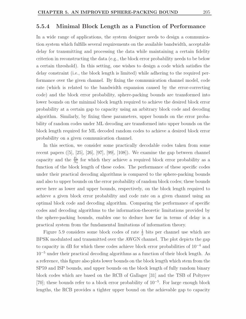
CHAPTER 5. AN IMPROVED SPHERE-PACKING BOUND 205
5.5.4 Minimal Block Length as a Function of Performance
In a wide range of applications, the system designer needs to design a communica-
tion system which fulfills several requirements on the available bandwidth, acceptable
delay for transmitting and processing the data while maintaining a certain fidelity
criterion in reconstructing the data (e.g., the block error probability needs to be below
a certain threshold). In this setting, one wishes to design a code which satisfies the
delay constraint (i.e., the block length is limited) while adhering to the required per-
formance over the given channel. By fixing the communication channel model, code
rate (which is related to the bandwidth expansion caused by the error-correcting
code) and the block error probability, sphere-packing bounds are transformed into
lower bounds on the minimal block length required to achieve the desired block error
probability at a certain gap to capacity using an arbitrary block code and decoding
algorithm. Similarly, by fixing these parameters, upper bounds on the error proba-
bility of random codes under ML decoding are transformed into upper bounds on the
block length required for ML decoded random codes to achieve a desired block error
probability on a given communication channel.
In this section, we consider some practically decodable codes taken from some
recent papers ([5], [25], [26], [97], [99], [108]). We examine the gap between channel
capacity and the Eb
N0for which they achieve a required block error probability as a
function of the block length of these codes. The performance of these specific codes
under their practical decoding algorithms is compared to the sphere-packing bounds
and also to upper bounds on the error probability of random block codes; these bounds
serve here as lower and upper bounds, respectively, on the block length required to
achieve a given block error probability and code rate on a given channel using an
optimal block code and decoding algorithm. Comparing the performance of specific
codes and decoding algorithms to the information-theoretic limitations provided by
the sphere-packing bounds, enables one to deduce how far in terms of delay is a
practical system from the fundamental limitations of information theory.
Figure 5.9 considers some block codes of rate 12
bits per channel use which are
BPSK modulated and transmitted over the AWGN channel. The plot depicts the gap
to capacity in dB for which these codes achieve block error probabilities of 10−4 and
10−5 under their practical decoding algorithms as a function of their block length. As
a reference, this figure also plots lower bounds on the block length which stem from the
SP59 and ISP bounds, and upper bounds on the block length of fully random binary
block codes which are based on the RCB of Gallager [31] and the TSB of Poltyrev
[70]; these bounds refer to a block error probability of 10−5. For large enough block
lengths, the RCB provides a tighter upper bound on the achievable gap to capacity

CHAPTER 5. AN IMPROVED SPHERE-PACKING BOUND 206
102
103
104
105
106
107
0
0.5
1
1.5
2
2.5
3
Block length [Bit]
∆ E
b/N0 [d
B]
min(RCB,TSB)max(ISP,SP59)
Pe = 10−5
Pe = 10−4RCB
RCB
TSB
ISP
ISP
SP59
SP59
4
1
2
3
Channel: AWGNModulation: BPSKRate: 0.5 bits/channel use
Figure 5.9: This figure refers to the tradeoff between the block length and the gapto capacity of error-correcting codes which are BPSK modulated and transmitted
over an AWGN channel. The horizontal axis refers to the block length of the codes,and the vertical axis refers to the gap, measured in decibels, between the channelcapacity and the energy per bit to spectral noise density (Eb
N0) which is required to
obtain a block error probability Pe (set either to 10−4 or 10−5). The considered rateof all the codes is one-half bit per channel use. The minimal gap to capacity whichis required for achieving a block error probability of 10−5 is depicted via bounds:the upper bound is calculated using the random-coding bound (RCB) of Gallager
[31] and the tangential-sphere bound (TSB) of Poltyrev [70] applied to fully randomand binary block codes, and the lower bound on this minimal block length iscalculated via the 1959 sphere-packing (SP59) bound of Shannon [89] and theimproved sphere-packing (ISP) bound introduced in Section 5.3. In addition to
bounds, this tradeoff between the block length (delay) and gap to capacity, is shownfor some efficiently decodable error-correcting codes; the codes are taken from [108]
(code 1), [26] (codes 2 and 4) and [25] (code 3).

CHAPTER 5. AN IMPROVED SPHERE-PACKING BOUND 207
than the TSB; this is expected since the error exponent of the TSB is slightly looser
than the random-coding error exponent (see [104, upper plot of Fig. 3]). However, for
small to moderate block lengths (i.e., for block lengths below approximately 5000 bits
according to Figure 5.9), the TSB provides a tighter upper bound on the achievable
gap as compared to the RCB. The improvement of the TSB over the RCB closes the
gap between the upper and lower bounds on the achievable gap to capacity for small
to moderate block lengths (where the lower bound is obtained via the SP59 bound
which is tighter than the ISP bound for the considered range of block lengths). As
for particularly efficient block codes, the code labeled 1 in Figure 5.9 is a block code
of length 192 bits which is decoded using a near-ML decoder by applying ‘box and
match’ decoding techniques [108]. It is observed that this code outperforms RCB for
ML decoded random codes with the same block length and code rate, and almost
coincides with the upper bound obtained via the TSB. It is also observed that this
code achieves a block error probability of 10−5 at a gap to capacity of 2.76 dB while the
SP59 bound gives that the block length required to achieve this performance is lower
bounded by 133 bits (so the bound is very informative). The codes labeled 2, 3 and
4 are prototype-based LDPC codes of lengths 2048, 5176 and 8192 bits, respectively
(codes 2 and 4 are taken from [26] and code 3 is taken from [25]). These codes
achieve under iterative decoding a block error probability of 10−5 at gaps to capacity
of 1.70, 1.27 and 1.07 dB, respectively. In terms of block length, the gap between the
performance of these codes under iterative decoding and the SP59 lower bound on
the block length required to achieve a block error probability of 10−5 at these channel
conditions is less than one order of magnitude. It is also noted that throughout the
range of block lengths depicted in Figure 5.9, the gap between the lower bound on the
block length of optimal codes which stems from the better of the two sphere-packing
bounds and the upper bound on the block length of random codes is less than one
order of magnitude. This exemplifies the tightness of the sphere-packing bounds when
used as lower bounds on the block lengths of optimal codes.
Figure 5.10 considers some LDPC codes of rate 0.88 bits per channel use which
are BPSK modulated and transmitted over the AWGN channel. The gap to capacity
in dB for which these codes achieve block error probabilities of 10−4 and 10−5 under
iterative decoding is plotted as a function of block length. As in Figure 5.9, the
figure uses upper and lower bounds on the achievable gap to capacity in terms of
the block length: for this (relatively high) code rate and the considered range of
block lengths, the ISP bound is uniformly tighter than the SP59 bound (so only the
ISP bound is depicted in this figure, and the SP59 bound is omitted). The upper
bounds on the required block lengths for achieving a target block error probability
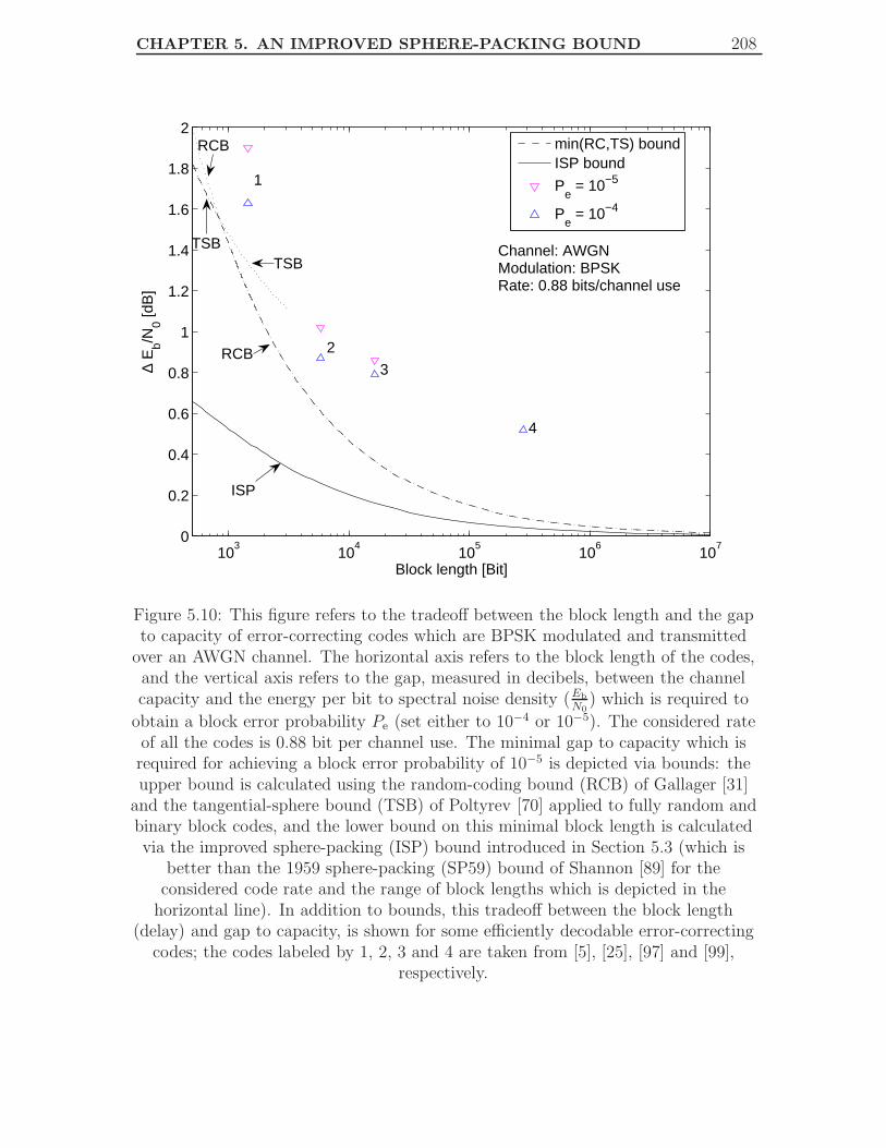
CHAPTER 5. AN IMPROVED SPHERE-PACKING BOUND 208
103
104
105
106
107
0
0.2
0.4
0.6
0.8
1
1.2
1.4
1.6
1.8
2
Block length [Bit]
∆ E
b/N0 [d
B]
min(RC,TS) boundISP bound
Pe = 10−5
Pe = 10−4
TSB
RCB
TSB
RCB
1
2
3
4
Channel: AWGNModulation: BPSKRate: 0.88 bits/channel use
ISP
Figure 5.10: This figure refers to the tradeoff between the block length and the gapto capacity of error-correcting codes which are BPSK modulated and transmitted
over an AWGN channel. The horizontal axis refers to the block length of the codes,and the vertical axis refers to the gap, measured in decibels, between the channelcapacity and the energy per bit to spectral noise density (Eb
N0) which is required to
obtain a block error probability Pe (set either to 10−4 or 10−5). The considered rateof all the codes is 0.88 bit per channel use. The minimal gap to capacity which isrequired for achieving a block error probability of 10−5 is depicted via bounds: theupper bound is calculated using the random-coding bound (RCB) of Gallager [31]
and the tangential-sphere bound (TSB) of Poltyrev [70] applied to fully random andbinary block codes, and the lower bound on this minimal block length is calculatedvia the improved sphere-packing (ISP) bound introduced in Section 5.3 (which is
better than the 1959 sphere-packing (SP59) bound of Shannon [89] for theconsidered code rate and the range of block lengths which is depicted in the
horizontal line). In addition to bounds, this tradeoff between the block length(delay) and gap to capacity, is shown for some efficiently decodable error-correcting
codes; the codes labeled by 1, 2, 3 and 4 are taken from [5], [25], [97] and [99],respectively.

CHAPTER 5. AN IMPROVED SPHERE-PACKING BOUND 209
in terms of the achievable gap to capacity are obtained via the RCB and the TSB
when it is applied to the ensemble of fully random block codes. The upper and lower
bounds refer to a block error probability of 10−5. Similarly to Figure 5.9, the RCB
is advantageous over the TSB for block codes of short to moderate block lengths; in
this case, the advantage of the RCB over the TSB occurs for block lengths above
approximately 1000 bits (instead of 5000 bits, as was the case in Fig. 5.9 for code
rate of 0.5 bit per channel use). This shows that for short block lengths, the TSB is
tighter than the RCB; however, since by increasing the code rate, the error exponent
of the TSB becomes less tight as compared to the error exponent of the RCB (see
the upper and lower plots of [104, Fig. 3] which refers to code rates of 0.5 and 0.9
bits per channel use), the asymptotic advantage of the RCB over the TSB is more
pronounced, and the former bound is tighter than the latter already for shorter block
lengths. The tradeoff between the gap to capacity (in terms of Eb
N0) versus the block
length is depicted in Figure 5.10 for some efficient error-correcting codes, in order to
compare their practical performance and delay to the information-theoretic bounds
(similarly to Fig. 5.9). For the examined block error probabilities (of 10−4 and 10−5),
the depicted codes require a gap to capacity of between 0.63 and 1.9 dB. For this range
of Eb
N0, the lower bound on the block lengths which is derived from the ISP bound is
looser than the one given by the SP59 bound. However, both bounds are not very
informative in this range. For cases where the gap to capacity is below 0.5 dB, the
difference between the lower bound on the block length of optimal codes which stems
from the ISP bound and the upper bound on the block length of random codes is less
than one order of magnitude. Code number 1 is an LDPC of length 1448 bits whose
construction of is based on balanced incomplete block designs [5]. This code achieves
a block error probability of 10−5 at a gap to capacity of 1.9 dB while the RCB shows
that the block length which is required to achieve this performance using random
codes is upper bounded by 600 bits. The code labeled 2 is a prototype-based LDPC
code of length 5176 bits which is taken from [25]. Code number 3 is a quasi-cyclic
LDPC code of length 16362 bits taken from [97]. These code achieve under iterative
decoding a block error probability of 10−5 at gaps to capacity of 1.02 and 0.86 dB,
respectively. In terms of block length, the gap between the performance of these codes
under iterative decoding and the upper bound on the block length of random codes
which achieve a block error probability of 10−5 under the same channel conditions is
less than one order of magnitude. The code labeled 4 is a finite-geometry LDPC code
of length 279552 bits which is taken from [99]. For this code we only have the gap
to capacity required to achieve a block error probability of 10−4, however, it is clear
that the difference in block length from the RCB becomes quite large as the gap to

CHAPTER 5. AN IMPROVED SPHERE-PACKING BOUND 210
capacity is reduced.
By fixing the block length and considering the gap in ∆Eb/N0 between the perfor-
mance of the specific codes and the sphere-packing bounds in Figures 5.9 and 5.10, it
is observed that the codes considered in these plots exhibit gaps of 0.2–0.8 dB w.r.t.
the information-theoretic limitation provided by the sphere-packing bounds (with the
exception of code 1 in Figure 5.10 which exhibits a gap of about 1.25 dB). In this re-
spect we also mention that some high rate turbo-product codes with moderate block
lengths (see [21]) exhibit a gap of 0.75 – 0.95 dB w.r.t. the information-theoretic
limitation provided by the ISP bound. Based on numerical results in [105] for the
ensemble of uniformly interleaved (1144, 1000) turbo-block codes whose components
are random systematic, binary and linear block codes, the gap in Eb
N0between the ISP
lower bound and an upper bound under ML decoding is 0.9 dB for a block error prob-
ability of 10−7. These results exemplify the strength of the sphere-packing bounds
for assessing the theoretical limitations of block codes and the power of iteratively
decoded codes (see also [27, 44, 45, 79, 109]).
5.6 Summary
This paper presents an improved sphere-packing (ISP) bound for finite-length block
codes whose transmission takes place over symmetric memoryless channels. The im-
proved tightness of the bound is especially pronounced for codes of short to moderate
block lengths, and some of its applications are exemplified in this paper. The deriva-
tion of the ISP bound was stimulated by the remarkable performance and feasible
complexity of turbo-like codes with short to moderate block lengths. We were mo-
tivated by recent improvements on the sphere-packing bound of [87] for finite block
lengths, as suggested by Valembois and Fossorier [109].
We first review the classical sphere-packing bounds, i.e., the 1959 sphere-packing
bound (SP59) derived by Shannon for equal-energy signals transmitted over the
Gaussian channel [89], and the 1967 sphere-packing (SP67) bound derived by Shan-
non, Gallager and Berlekamp for discrete memoryless channels [87]. The ISP bound,
introduced in Section 5.3, is uniformly tighter than the classical SP67 bound [87] and
the bound in [109].
We apply the ISP bound to various memoryless symmetric channels. The tightness
of the ISP bound is exemplified by comparing it with upper and lower bounds on the
ML decoding error probability and also with reported computer simulations of turbo-
like codes under iterative decoding.
This paper also presents a new numerical algorithm which performs the entire

CHAPTER 5. AN IMPROVED SPHERE-PACKING BOUND 211
calculation of the SP59 bound in the logarithmic domain, thus facilitating the exact
calculation of the SP59 bound for all block lengths without the need for asymptotic
approximations. It is shown that the ISP bound suggests an interesting alternative
to the SP59 bound, where the latter is specialized for the AWGN channel.
In a wide range of applications, one wishes to design a block code which satisfies a
known delay constraint (i.e., the block length is limited) while adhering to a required
performance over a given channel model. By fixing the communication channel model,
code rate and the block error probability, sphere-packing bounds are transformed into
lower bounds on the minimal block length required to achieve the target block error
probability at a certain gap to capacity when an arbitrary block code and decod-
ing algorithm are used. Comparing the performance of specific codes and decoding
algorithms to the information-theoretic limitations provided by the sphere-packing
bounds, enables one to deduce how far in terms of delay is a practical system from
the fundamental limitations of information theory. Further details on the compari-
son between practically decodable codes and the sphere-packing bounds are found in
Section 5.5.4.
The ISP bound is especially attractive for block codes of short to moderate block
lengths, and its advantage is especially pronounced for high rate codes. Its improve-
ment over the SP67 bound and the bound in [109, Theorem 7] also becomes more
significant as the input alphabet of the considered modulation is increased.
Appendices
5.A Proof of Lemma 5.1
We consider a symmetric DMC with input alphabet K = 0, . . . , K − 1, output
alphabet J = 0, . . . J − 1 (where J, K ∈ N) and a transition probability function
P (·|·). Let gkKk=0 be the set of unitary functions which satisfy the conditions (5.24)
and (5.25) in Definition 5.2. To prove Lemma 5.1, we start with a discussion on the
distribution qs which satisfies (5.48).
On the input distribution qs for symmetric DMCs
Lemma 5.A.1 For symmetric DMCs and an arbitrary value of s ∈ (0, 1), the uni-
form distribution qk,s = 1K
for k ∈ K satisfies (5.48) with equality.

CHAPTER 5. AN IMPROVED SPHERE-PACKING BOUND 212
Proof: To prove the lemma, it is required to show that
J−1∑
j=0
P (j|k)1−s
(K−1∑
k′=0
1
KP (j|k′)1−s
) s1−s
=J−1∑
j=0
(K−1∑
k′=0
1
KP (j|k′)1−s
) 11−s
, ∀k ∈ K. (5.A.1)
Let us consider some k ∈ K. Examining the left-hand side (LHS) of (5.A.1) gives
J−1∑
j=0
P (j|k)1−s
(K−1∑
k′=0
1
KP (j|k′)1−s
) s1−s
= KJ−1∑
j=0
1
KP (j|k)1−s
(K−1∑
k′=0
1
KP (j|k′)1−s
) s1−s
(a)=
K−1∑ek=0
J−1∑
j=0
1
KP (j|k)1−s
(K−1∑
k′=0
1
KP (j|k′)1−s
) s1−s
(b)=
K−1∑ek=0
J−1∑
j=0
1
KP (gek(j)|k)1−s
(K−1∑
k′=0
1
KP (gek(j)|k′)1−s
) s1−s
(5.A.2)
where (a) holds by summing over a dummy variable k ∈ K instead of the multipli-
cation by K in the previous line, and (b) holds since gek is unitary for all k ∈ K (see
(5.23) where the integral is replaced here by a sum). For all j ∈ J and k ∈ K, the
symmetry properties in (5.24) - (5.26) give
P(gek(j)| k) (a)
= P((
g−1k gek)(j)| 0)
(b)= P
(g(ek−k)modK
(j)| 0)
(c)= P
(j| (k − k)modK
)(5.A.3)
where (a) follows from (5.24), (b) relies on (5.25), and (c) follows from (5.24) and
(5.26). Similarly, for all j, k ∈ 0, 1, . . . , K − 1K−1∑
k′=0
1
KP (gek(j)|k′)1−s (a)
=K−1∑
k′=0
1
KP(j| (k′ − k)modK
)1−s
(b)=
K−1∑
k′=0
1
KP (j|k′)1−s (5.A.4)
where (a) relies on (5.A.3) and (b) holds since when the index k′ takes all the values in
0, 1, . . . , K − 1, so does (k′ − k)modK. Substituting (5.A.3) and (5.A.4) in (5.A.2)

CHAPTER 5. AN IMPROVED SPHERE-PACKING BOUND 213
gives
J−1∑
j=0
P (j|k)1−s
(K−1∑
k′=0
1
KP (j|k′)1−s
) s1−s
=K−1∑ek=0
J−1∑
j=0
1
KP(j|(k − k)modK
)1−s
(K−1∑
k′=0
1
KP (j|k′)1−s
) s1−s
=
J−1∑
j=0
K−1∑ek=0
1
KP(j|(k − k)modK
)1−s
(
K−1∑
k′=0
1
KP (j|k′)1−s
) s1−s
(a)=
J−1∑
j=0
K−1∑ek=0
1
KP (j|k)1−s
(
K−1∑
k′=0
1
KP (j|k′)1−s
) s1−s
=
J−1∑
j=0
(K−1∑
k′=0
1
KP (j|k′)1−s
) 11−s
(5.A.5)
where equality (a) holds since the k takes all the values in 0, 1, . . . , K − 1, and so
does the index k′ , (k − k)modK.
We now turn to explore how the symmetry of the channel and the input distribution
qs induce a symmetry on the probability tilting measure fs.
On the symmetry of the tilting measure fs for strictly symmetric DMCs
Lemma 5.A.2 For all s ∈ (0, 1), k ∈ K and j ∈ J , the tilting measure fs in (5.50)
satisfies
fs(j) = fs
(gk(j)
). (5.A.6)
Proof: Examining the definition of fs in (5.50), it can be observed that it suffices to
show that
αj,s = αgk(j),s , ∀s ∈ (0, 1), k ∈ K, j ∈ J (5.A.7)
where αj,s is given in (5.49). Note that for the uniform input distribution where qk,s =1K
for all k ∈ K, inequalities (5.48) and (5.49) hold with equality (see Lemma 5.A.1).
From (5.A.4), equality (5.A.7) follows for the uniform input distribution.
Having established some symmetry properties of qs and fs, we are ready to prove
equalities (5.51) – (5.53).

CHAPTER 5. AN IMPROVED SPHERE-PACKING BOUND 214
On the independence of µk and its two derivatives from k As we have shown,
the uniform distribution qs satisfies (5.48) in equality for all inputs, so
µk(s) = ln
(∑
j
P (j|k)1−sfs(j)s
)
(a)= ln
(∑
j
P (j|k)1−s (αj,s)s
1−s
)− s ln
(∑
j
(αj,s)1
1−s
)
(b)= (1 − s) ln
(∑
j
(αj,s)1
1−s
)
(c)= (1 − s) ln
∑
j
[∑
k
qk,sP (j|k)1−s
] 11−s
(5.A.8)
where (a) follows from the choice of fs in (5.49) and (5.50), (b) follows from Lemma 5.A.1
and (5.49), and (c) follows from (5.49). Under the setting s = ρ
1+ρ, since the condi-
tions on qs in (5.48) are identical to the conditions on the input distribution q = qs
which maximizes E0(s
1−s,q) as stated in [31, Theorem 4], then
µk(s, fs) = (1 − s) ln
∑
j
[∑
k
qk,sP (j|k)1
1+ s1−s
]1+ s1−s
= −(1 − s) E0
(s
1 − s,qs
)
= −(1 − s) E0
(s
1 − s
), 0 < s < 1 (5.A.9)
where E0 is given in (5.19). This proves (5.51).
We now turn to prove the independence of the first two derivatives of µk w.r.t s
from k ∈ K.
Remark 5.11 Note that the partial derivative of µk(s) w.r.t s is performed while
holding f = fs constant.
As is shown in [87],
µ′(s) = EQs
(D(j)
)
µ′′(s) = VarQs
(D(j)
)
where
D(j) , ln
(P2(j)
P1(j)
), Qs(j) ,
P1(j)1−sP2(j)
s
∑j′ P1(j′)1−sP2(j′)s
.

CHAPTER 5. AN IMPROVED SPHERE-PACKING BOUND 215
For every k ∈ K, P1 and P2 used in µk are defined to be P (·|k) and fs, respectively.
Hence, for all k ∈ K
µ′k(s, fs) = EQk,s
(Dk,s(j)
)
µ′′k(s, fs) = VarQk,s
(Dk,s(j)
)(5.A.10)
where
Dk,s(j) , ln
(fs(j)
P (j|k)
)(5.A.11)
Qk,s(j) ,P (j|k)1−sfs(j)
s
J−1∑
j′=0
P (j′|k)1−sfs(j′)s
. (5.A.12)
Applying (5.24) and Lemma 5.A.2, we get that for all k ∈ KJ−1∑
j′=0
P (j′|k)1−sfs(j′)s (a)
=J−1∑
j′=0
P (g−1k (j′)|0)1−sfs(g
−1k (j′))s
(b)=
J−1∑
j′=0
P (j′|0)1−sfs(j′)s (5.A.13)
where (a) follows from (5.24) and Lemma 5.A.2, and (b) follows since g−1k is unitary.
Substituting (5.A.13) in (5.A.12) gives
Qk,s(j) =P (j|k)1−sfs(j)
s
J−1∑
j′=0
P (j′|k)1−sfs(j′)s
(a)=
P (g−1k (j)|0)1−sfs(g
−1k (j))s
J−1∑
j′=0
P (j′|0)1−sfs(j′)s
(b)= Q0,s
(g−1
k (j))
(5.A.14)
where (a) follows from (5.24), (5.26), (5.50), (5.A.6) and (5.A.13), and (b) relies on
the definition of Qk,s in (5.A.12). Similarly,
Dk,s(j) = ln
(fs(j)
P (j|k)
)
(a)= ln
(fs
(g−1
k (j))
P(g−1
k (j)|0))
(b)= D0,s
(g−1
k (j))
(5.A.15)

CHAPTER 5. AN IMPROVED SPHERE-PACKING BOUND 216
where (a) follows from (5.24), (5.26) and (5.A.6), and (b) relies on the definition of
Dk,s in (5.A.11). Using (5.A.14) and (5.A.15), we finally get for all k ∈ K
µ′k(s) = EQk,s
(Dk,s(j)
)
=J−1∑
j=0
Qk,s(j)Dk,s(j)
=
J−1∑
j=0
Q0,s
(g−1
k (j))D0,s
(g−1
k (j))
(a)=
J−1∑
j=0
Q0,s(j)D0,s(j)
= µ′0(s)
and
µ′′k(s) = VarQk,s
(Dk,s(j)
)
=
J−1∑
j=0
Qk,s(j)D2k,s(j) − µ′
k(s)2
=J−1∑
j=0
Q0,s
(g−1
k (j))(
D0,s
(g−1
k (j)))2
− µ′0(s)
2
(b)=
J−1∑
j=0
Q0,s(j)(D0,s(j)
)2 − µ′0(s)
2
= µ′′0(s)
where (a) and (b) follow since g−1k is unitary for all k ∈ K. This completes the proof
of Lemma 5.1.
Remark 5.12 Equalities (5.51)–(5.53) hold for arbitrary symmetric memoryless chan-
nels. For a general output alphabet J ⊆ Rd, the proof of these properties follows the
same lines as the proof here with the exception that the sums over J are replaced by
integrals. As in Definition 5.1, if the projection of J over some of the d dimensions
is countable, the integration over these dimensions is turned into a sum.

CHAPTER 5. AN IMPROVED SPHERE-PACKING BOUND 217
5.B Calculation of the Function µ0 in (5.47) for some
Symmetric Channels
This appendix presents some technical calculations which yield the expressions for
the function µ0 defined in (5.47) and its first two derivatives w.r.t. s (while holding
fs fixed in the calculation of the partial derivatives of µ w.r.t. s, as required in
[87]). The examined cases are M-ary PSK modulated signals transmitted over fully
interleaved fading channels, with the AWGN channel as a special case, and binary
block codes transmitted over the BEC. These expressions serve for the application
of the VF bound in [109] and the ISP bound derived in Section 5.3 to block codes
transmitted over these channels.
5.B.1 M-ary PSK Modulated Signal over Fully Interleaved
Fading Channels with Perfect CSI
For M-ary PSK modulated signals transmitted over a fully interleaved fading channel,
the channel output is J = R2×R
+, where the first two coordinates refer to the vector
Y and the third refers to the fading coefficient A. In the case of a continuous output
alphabet, the sums in (5.A.8) are replaced by integrals, and the transition probabilities
are replaced by transition probability density functions. To simplify the presentation,
for all s ∈ (0, 1), y ∈ R2 and a ∈ R
+ we define
κs(y, a) ,
(1
M
M−1∑
k=0
e(1−s)a 〈y,xk−x0〉
σ2
) 11−s
. (5.B.1)
This expression will be used throughout the following calculations.
Due to the symmetry of the channel, we get from Lemma 5.A.1 that the distrib-
ution qs which satisfies (5.48) is uniform. Hence, we get by substituting (5.80) into
(5.A.8) that
µ0(s) = (1 − s) ln
∫∫
R2
∞∫
0
pA(a)
2πσ2e−
‖y−ax0‖22σ2 ζs(y, a)da dy
where
ζs(y, a) ,
(1
M
M−1∑
k=0
e−(1−s)(‖y−axk‖2−‖y−ax0‖2)
2σ2
) 11−s
Since ‖xk‖2 = 1 for all k ∈ 0, 1, . . . , M − 1 we have
‖y − axk‖2 − ‖y − ax0‖2 = −2a〈y,xk − x0〉 (5.B.2)

CHAPTER 5. AN IMPROVED SPHERE-PACKING BOUND 218
and so µ0 can be rewritten in the form
µ0(s) = (1 − s) ln (θ(s))
where
θ(s) ,
∫∫
R2
∞∫
0
pA(a)
2πσ2e−
‖y−ax0‖22σ2 κs(y, a)da dy. (5.B.3)
and κs(y, a) is defined in (5.B.1).
We now turn to calculate the derivative of µ0 with respect to s while holding
f = fs constant. Substituting (5.80) into the definition of fs in (5.50), we get that fs
is given by
fs(y, a) =
(M−1∑
k=0
1
M
(pA(a)
2πσ2
)1−s
e−(1−s) ‖y−axk‖2
2σ2
) 11−s
∫∫
R2
∞∫
0
(M−1∑
k=0
1
M
(pA(a′)
2πσ2
)1−s
e−(1−s) ‖y′−a′xk‖2
2σ2
) 11−s
da′dy′
=κs(y, a)
θ(s)
pA(a)
2πσ2e−
‖y−ax0‖22σ2 (5.B.4)
where the last equality follows from (5.B.2) and (5.B.3). The log-likelihood ratio D0,s
in (5.A.11) is given by
D0,s(y, a) , ln
(fs(y, a)
P (y, a|0)
)
= ln(κs(y, a)
)− ln
(θ(s)
)(5.B.5)
where the second equality follows from (5.80) and (5.B.4). The distribution Q0,s in
(5.A.12) is given by
Q0,s(y, a)
,P (y, a|0)1−sfs(y, a)s
∫∫
R2
∞∫
0
P (y′, a′|0)1−sfs(y′, a′)s da′ dy′
=
pA(a)
2πσ2e−
‖y−ax0‖22σ2
(κs(y, a)
)s
∫∫
R2
∞∫
0
pA(a′)
2πσ2e−
‖y′−a′x0‖2
2σ2(κs(y, a′)
)sda′dy′

CHAPTER 5. AN IMPROVED SPHERE-PACKING BOUND 219
(a)=
pA(a)
2πσ2e−
‖y−ax0‖22σ2
(κs(y, a)
)s
·
∫∫
R2
∞∫
0
(1
M
M−1∑
k=0
(1
2πσ2e−
‖y′−a′xk‖2
2σ2
)1−s) s
1−s(pA(a′)
2πσ2e−
‖y′−a′x0‖2
2σ2
)1−s
da′ dy′
−1
(b)=
pA(a)
2πσ2e−
‖y−ax0‖22σ2
(κs(y, a)
)s
∫∫
R2
∞∫
0
(1
M
M−1∑
k=0
(pA(a′)
2πσ2e−
‖y′−a′xk‖2
2σ2
)1−s) 1
1−s
da′dy′
(c)=
pA(a)
2πσ2e−
‖y−ax0‖22σ2
(κs(y, a)
)s
∫∫
R2
∞∫
0
pA(a′)
2πσ2e−
‖y′−a′x0‖2
2σ2 κs(y, a′) da′dy′
(d)=
pA(a) (κs(y, a))s
2πσ2 θ(s)e−
‖y−ax0‖22σ2 (5.B.6)
where (a) and (c) rely on (5.B.2), (b) follows from Lemma 2.1 in the proof for symmet-
ric memoryless channels, and (d) relies on the definition of θ in (5.B.3). Substituting
(5.B.5) and (5.B.6) in (5.A.10) we get
µ′0(s) = EQ0,s
(D0,s
)
=1
θ(s)
∫∫
R2
∞∫
0
pA(a)
2πσ2e−
‖y−ax0‖22σ2
(κs(y, a)
)s
· ln(κs(y, a)
)da dy − ln
(θ(s)
)(5.B.7)
and
µ′′0(s) = EQ0,s
(D2
0,s(y))− µ′
0(s)2
=1
θ(s)
∫∫
R2
∞∫
0
pA(a)
2πσ2e−
‖y−ax0‖22σ2
(κs(y, a)
)s
·(
ln(κs(y, a)
)− ln
(θ(s)
))2
da dy
−µ′0(s)
2 . (5.B.8)
In this paper, we consider the particular case where the fading coefficients have a
Rayleigh distribution. In this case, the distribution of the fading samples is given by
pA(a) = 2a e−a2for a ≥ 0, so that E(A2) = 1.

CHAPTER 5. AN IMPROVED SPHERE-PACKING BOUND 220
5.B.2 M-ary PSK Modulated Signals over the AWGN Chan-
nel
A widely studied special case of fully interleaved fading channels is the AWGN channel
where the fading coefficients are set to 1. Substituting PA(a) = δ(a − 1), where δ is
the Dirac delta function at zero, we get that θ in (5.B.3) is particularized to
θ(s) ,
∫∫
R2
e−‖y−x0‖2
2σ2
2πσ2κs(y, a) dy (5.B.9)
and the first and second derivatives of µ0 w.r.t. s (while holding fs constant) are
given by
µ′0(s) =
1
θ(s)
∫∫
R2
e−‖y−x0‖2
2σ2
2πσ2
(κs(y, a)
)sln(κs(y, a)
)dy − ln
(θ(s)
)(5.B.10)
and
µ′′0(s) =
1
θ(s)
∫∫
R2
1
2πσ2e−
‖y−x0‖22σ2
(κs(y, a)
)s(ln(κs(y, a)
)− ln
(θ(s)
))2
dy − µ′0(s)
2 .
(5.B.11)
5.B.3 The Binary Erasure Channel
Let us denote the output of the channel when an erasure has occurred by E , and let
p designate the erasure probability of the channel. Since the BEC is symmetric, the
input distribution qs which satisfies (5.48) is uniform (see Lemma 5.A.1), and we get
from (5.A.8)
µ0(s, fs) = (1 − s) ln
(2(1 − p)
21
1−s
+ p
)
= (1 − s) ln(2(1 − p) + 2
11−s p
)− ln 2 . (5.B.12)
We now turn to calculate fs for the BEC; substituting the transition probabilities
into (5.50) gives
fs(0) = fs(1) =
(12(1 − p)1−s
) 11−s
2(
12(1 − p)1−s
) 11−s + (p1−s)
11−s
=2−
11−s (1 − p)
21− 11−s (1 − p) + p
=1 − p
2(1 − p) + 21
1−s p(5.B.13)

CHAPTER 5. AN IMPROVED SPHERE-PACKING BOUND 221
and
fs(E) =(p1−s)
11−s
2(
12(1 − p)1−s
) 11−s + (p1−s)
11−s
=p
21− 11−s (1 − p) + p
=2
11−s p
2(1 − p) + 21
1−s p. (5.B.14)
Substituting (5.B.13) and (5.B.14) into the definition of the distribution Q0,s in
(5.A.12) gives
Q0,s(0) =P (0|0)1−sfs(0)s
∑
j∈0,1,EP (j|0)1−sfs(j)
s=
1 − p
1 − p + 2s
1−s p
Q0,s(1) =P (1|0)1−sfs(0)s
∑
j∈0,1,EP (j|0)1−sfs(j)
s= 0
Q0,s(E) =P (E|0)1−sfs(E)s
∑
j∈0,1,EP (j|0)1−sfs(j)
s=
2s
1−s p
1 − p + 2s
1−s p(5.B.15)
and the LLR in (5.A.11) is given by
D0,s(0) = ln
(1
2(1 − p) + 21
1−s p
)
D0,s(E) = ln
(2
11−s
2(1 − p) + 21
1−s p
). (5.B.16)
Applying (5.B.15) and (5.B.16) we get from (5.A.12)
µ′0(s, fs) = EQ0,s
(D0,s
)
=1 − p
1 − p + 2s
1−s pln
(1
2(1 − p) + 21
1−s p
)
+2
s1−s p
1 − p + 2s
1−s pln
(2
11−s
2(1 − p) + 21
1−s p
)
= ln
(1
1 − p + 2s
1−s p
)+
2s
1−s p
1 − p + 2s
1−s p
ln 2
1 − s(5.B.17)

CHAPTER 5. AN IMPROVED SPHERE-PACKING BOUND 222
and
µ′′0(s, fs) = EQ0,s
(D2
0,s
)− µ′
0(s, fs)2
=1 − p
1 − p + 2s
1−s pln2
(1
2(1 − p) + 21
1−s p
)
+2
s1−s p
1 − p + 2s
1−s pln2
(2
11−s
2(1 − p) + 21
1−s p
)− µ′
0(s, fs)2
= ln2
(1
1 − p + 2s
1−s p
)+
2s
1−s p
1 − p + 2s
1−s p
(ln 2
1 − s
)2
+2
11−s p
1 − p + 2s
1−s p
ln 2
1 − sln
(1
1 − p + 2s
1−s p
)− µ′
0(s, fs)2
=2
s1−s p (1 − p)
(1 − p + 2
s1−s p
)2(
ln 2
1 − s
)2
(5.B.18)
5.C Proof of Proposition 5.3
From the definition of fN in (5.67), it follows that
fN(x) =1
2N−1
2 Γ(N+12
)
∫ ∞
0
zN−1 exp(−z2
2+ zx) dz
=exp
(x2
2
)
2N−1
2 Γ(N+12
)
∫ ∞
0
zN−1 exp
(−(z − x)2
2
)dz
=exp
(x2
2
)
2N−1
2 Γ(N+12
)
∫ ∞
−x
(u + x)N−1 exp
(−u2
2
)du .
From the binomial formula, we get
fN(x) =exp
(x2
2
)
2N−1
2 Γ(N+12
)
N−1∑
j=0
[(N − 1
j
)xN−1−j
∫ ∞
−x
uj exp
(−u2
2
)du
]. (5.C.1)
We now examine the integrals on the RHS of (5.C.1). For odd values of j, we get∫ ∞
−x
uj exp
(−u2
2
)du =
∫ x
−x
uj exp
(−u2
2
)du +
∫ ∞
x
uj exp
(−u2
2
)du
=
∫ ∞
x
uj exp
(−u2
2
)du
=
∫ ∞
0
uj exp
(−u2
2
)du −
∫ x
0
uj exp
(−u2
2
)du (5.C.2)
where the second equality follows since the integrand is an odd function for odd
values of j, and the interval of first integral is symmetric around zero (so this integral

CHAPTER 5. AN IMPROVED SPHERE-PACKING BOUND 223
vanishes). For even values of j, we get
∫ ∞
−x
uj exp
(−u2
2
)du =
∫ ∞
0
uj exp
(−u2
2
)du +
∫ 0
−x
uj exp
(−u2
2
)du
=
∫ ∞
0
uj exp
(−u2
2
)du +
∫ x
0
uj exp
(−u2
2
)du (5.C.3)
where the second equality holds since the integrand is an even function for even
values of j. Combining (5.C.2) and (5.C.3) gives that for j ∈ 0, 1, . . . , N − 1∫ ∞
−x
uj exp
(−u2
2
)du =
∫ ∞
0
uj exp
(−u2
2
)du + (−1)j
∫ x
0
uj exp
(−u2
2
)du
(a)=
∫ ∞
0
(2t)j−12 exp(−t) dt + (−1)j
∫ x2
2
0
(2t)j−12 exp(−t) dt
= 2j−12
∫ ∞
0
tj−12 exp(−t) dt
1 + (−1)j
∫ x2
2
0
tj−12 exp(−t) dt
∫ ∞
0
tj−12 exp(−t) dt
= 2j−12 Γ
(j + 1
2
) [1 + (−1)j γ
(x2
2,j + 1
2
)]
where (a) follows by substituting t , u2
2and the functions Γ and γ are introduced
in (5.75) and (5.76), respectively. Substituting the last equality in (5.C.1) and also
noting that(
N − 1
j
)=
Γ(N)
Γ(N − j) Γ(j + 1), N ∈ N, j ∈ 0, 1, . . . , N − 1
we get
fN(x) =exp
(x2
2
)
2N−1
2 Γ(N+12
)
N−1∑
j=0
Γ(N)
Γ(N − j) Γ(j + 1)xN−1−j 2
j−12
·Γ(
j + 1
2
) [1 + (−1)j γ
(x2
2,j + 1
2
)]
=N−1∑
j=0
exp(
x2
2
)
Γ(N − j)
Γ(N)
Γ(
N+12
) Γ(
j+12
)
Γ(j + 1)
xN−1−j
2N−j
2
[1 + (−1)j γ
(x2
2,j + 1
2
)]
(a)=
N−1∑
j=0
exp(
x2
2
)
Γ(N − j)
2N−1 Γ(
N2
)√
π
2−j√
π
Γ(
j
2+ 1) xN−1−j
2N−j
2
[1 + (−1)j γ
(x2
2,j + 1
2
)]
(b)=
N−1∑
j=0
exp(d(N, j, x)
)

CHAPTER 5. AN IMPROVED SPHERE-PACKING BOUND 224
where (a) follows from the equality
Γ(2u) =22u−1
√π
Γ(u) Γ
(u +
1
2
), u 6= 0,−1
2,−1,−3
2, . . .
and (b) follows from the definition of the function d in (5.74).

Chapter 6
Summary and Outlook
This research work focuses on the fundamental tradeoff between the performance of
graph-based codes and the complexity required to achieve this performance under
iterative message-passing decoding algorithms. The complexity of message-passing
algorithms is dictated by two main factors – the complexity of a single decoding
iteration and the number of iterations required to achieve the desired performance
level. In this work, we derive lower bounds on both of these factors. These bounds
refer to the asymptotic case where we let the block length of the codes tend to infinity.
We also consider the fundamental performance limitations of finite-length block codes.
This is done via the derivation of an improved sphere-packing (ISP) bound which
applies to block codes transmitted over memoryless symmetric channels.
6.1 Contributions of this Dissertation
In Chapter 2 we derive two types of bounds. The first category consists of lower
bounds on the asymptotic density of parity-check matrices of binary linear block
codes, which are given in terms of the gap between the code rate and the channel
capacity. Due to the nature of the iterative message-passing decoding algorithms,
these bounds serve as lower bounds on the complexity (per information bit) of a
single decoding iteration. The second category of bounds are upper bounds on the
achievable rates of binary linear block codes (even under maximum-likelihood (ML)
decoding). The bounds in both categories refer to the asymptotic case where we let
the block length of the codes tend to infinity and assume that the transmission takes
place over an arbitrary memoryless binary-input output-symmetric (MBIOS) channel.
The derivation of the bounds was motivated by the desire to tighten the statements
in [17, Theorems 1 and 2] and [81, Theorem 2.1]. The two-level quantization of
the information on the log-likelihood ratio (LLR) in [17, 81] in essence performs the
225

CHAPTER 6. SUMMARY AND OUTLOOK 226
analysis on a physically degraded binary symmetric channel (BSC) instead of the
original communication channel. As a first step, we present an analysis based on
information from a quantized channel which better reflects the statistics of the actual
communication channel (though the quantized information is still degraded w.r.t.
the original information provided by the channel). The number of quantization levels
applied to the information is set as an arbitrary integer power of 2. The calculation
of the bounds is subject to an optimization of the quantization levels of the LLR, as
to get the tightest bounds within their form. Later, we present bounds that rely on
the conditional pdf of the LLR at the output of the MBIOS channel, and perform the
analysis on an equivalent channel without a degradation of the channel information.
This second approach finally leads to bounds which are uniformly tighter than the
bounds based on a quantization of the communication channel. It appears to be even
simpler to calculate the un-quantized bounds, as their calculation does not involve
the solution of any optimization equation related to the quantization levels. The
comparison between the quantized and un-quantized bounds gives insight on the effect
of the number of quantization levels of the LLR (even if they are chosen optimally)
on the achievable rates, as compared to the ideal case where no quantization is done.
The information-theoretic bounds derived in Chapter 2 are valid for every se-
quence of binary linear block codes, in contrast to high probability results which
follow from probabilistic tools (e.g., density evolution (DE) analysis under iterative
message-passing decoding). The bounds hold under ML decoding, and hence, they
hold in particular under any sub-optimal decoding algorithm. We apply the bounds
to ensembles of low-density parity-check (LDPC) codes where the significance of these
bounds is as follows: Firstly, by comparing the new upper bounds on the achievable
rates with thresholds provided by DE analysis, we obtain rigorous bounds on the loss
in performance of various LDPC ensembles due to the sub-optimality of message-
passing decoding (as compared to ML decoding). Secondly, the parity-check density
of binary linear block codes which are represented by standard bipartite graphs is in-
terpreted as the complexity per iteration under message-passing decoding. Therefore,
by tightening the reported lower bound on the asymptotic parity-check density (see
[81, Theorem 2.1]), the new bounds provide better insight on the tradeoff between
the asymptotic performance and the asymptotic decoding complexity of iteratively
decoded LDPC codes. Thirdly, the new lower bound on the bit error probability of
binary linear block codes (see Corollary 2.4) tightens the reported lower bound in
[81, Theorem 2.5] and provides a quantitative measure to the number of fundamental
cycles in the graph which should exist in terms of the achievable rate (even under ML
decoding) and its gap to capacity. It is well known that cycle-free codes have poor

CHAPTER 6. SUMMARY AND OUTLOOK 227
performance [103], so the lower bound on the minimal number of fundamental cycles
in the graph (i.e., cycles which cannot be decomposed into some more elementary
cycles) as a function of the gap in rate to capacity strengthens the result in [103] on
the inherent limitation of cycle-free codes.
The lower bound on the asymptotic parity-check density in [81, Theorem 2.1] and
its improvements in Chapter 2 grow like the log of the inverse of the gap (in rate) to
capacity. The result in [81, Theorem 2.2] shows that a logarithmic growth rate of the
parity-check density is achievable for Gallager’s regular LDPC ensemble under ML
decoding when transmission takes place over an arbitrary MBIOS channel. These
results show that for any iterative decoder which is based on the representation of
the codes by Tanner graphs, there exists a tradeoff between asymptotic performance
and complexity which cannot be surpassed. Recently, it was shown in [64, 65] that a
better tradeoff can be achieved by allowing more complicated graphical models which
involve a sufficient number of state nodes in the graph; for the particular case of the
binary erasure channel (BEC), the encoding and the decoding complexity of properly
designed codes on graphs remains bounded as the gap to capacity vanishes.
The analysis in Chapter 3 generalizes the statements in Chapter 2 to the case
where the codes are transmitted over a set of statistically independent parallel MBIOS
channels. The bounds on the asymptotic achievable rates and parity-check density
can be applied to various scenarios which form particular cases of communication over
parallel channels, e.g., intentionally punctured LDPC codes [35], non-uniformly error
protected LDPC codes [69], and LDPC-coded modulation (see e.g., [37, 112]). In
Section 3.4, we use Theorem 3.1 for the derivation of upper bounds on the achievable
rates under ML decoding of (randomly and intentionally) punctured LDPC codes
whose transmission takes place over an MBIOS channel. It is exemplified numeri-
cally that for various good ensembles of intentionally punctured LDPC codes, the
asymptotic loss in performance due to the code structure is still non-negligible as
compared to the corresponding loss due to the sub-optimality of iterative decoding
(as compared to optimal ML decoding). Looser versions of the bounds derived in this
chapter for punctured LDPC codes suggest a simplified re-derivation of previously
reported bounds on the decoding complexity of randomly punctured LDPC codes
(see [65, Theorems 3 and 4]).
In Chapter 4, we turn to consider the number of iterations required for success-
ful decoding of graph-based code ensembles. In the considered setting, we let the
block length of these ensembles tend to infinity, and the transmission takes place over
a BEC. Theorems 4.1–4.3 demonstrate that for various attractive families of code

CHAPTER 6. SUMMARY AND OUTLOOK 228
ensembles (including LDPC codes, systematic and non-systematic irregular repeat-
accumulate (IRA) codes, and accumulate-repeat-accumulate (ARA) codes), the num-
ber of iterations which is required to achieve a desired bit erasure probability scales
at least like the inverse of the gap between the channel capacity and the design rate
of the ensemble. This conclusion holds provided that the fraction of degree-2 variable
nodes in the Tanner graph does not tend to zero as the gap to capacity vanishes
(where under mild conditions, this property is satisfied for sequences of capacity-
achieving LDPC ensembles, see [76, Lemma 5]). The behavior of these lower bounds
matches well with the experimental results and the conjectures on the number of
iterations and complexity, as provided by Khandekar and McEliece (see [42, 43, 56]).
In [42, Theorem 3.5], it was stated that for LDPC and IRA ensembles which achieve
a fraction 1−ε of the channel capacity of a BEC with a target bit erasure probability
of Pb under iterative message-passing decoding, the number of iterations grows like
O(
1ε
). In light of the outline of the proof of this statement, as suggested in [42, p. 71],
it implicitly assumes that the flatness condition is satisfied for these code ensembles
and also that the target bit erasure probability vanishes; under these assumptions,
the reasoning suggested by Khandekar in [42, Section 3.6] supports the behavior of
the lower bounds which are derived in this work.
The lower bounds on the number of iterations in Chapter 4 become trivial when
the fraction of degree-2 variable nodes vanishes. However, this is mainly a result
of our focus on the derivation of simple lower bounds on the number of iterations
which do not depend on the full characterization of the degree distributions of the
code ensembles. Following the proofs of the statements in this chapter and focusing
on the case where the fraction of degree-2 variable nodes vanishes, it is possible to
derive lower bounds on the number of iterations which are not trivial even in this
case; these bounds, however, require the knowledge of the entire degree distribution
of the examined ensembles.
To complement the asymptotic analysis in Chapters 2–4, we study the fundamen-
tal limitations on the performance of finite-length block codes. Chapter 5 presents an
improved sphere-packing (ISP) bound for finite-length block codes whose transmission
takes place over symmetric memoryless channels. The derivation of the ISP bound
was stimulated by the remarkable performance and feasible complexity of turbo-like
codes with short to moderate block lengths. We were motivated by recent improve-
ments on the 1967 sphere-packing (SP67) bound (see [87]) for finite block lengths,
as suggested by Valembois and Fossorier [109]. Numerical results demonstrate that
the ISP bound significantly tightens the SP67 bound and the bound in [109, Theo-
rem 7]. This improvement is especially pronounced for codes of short to moderate

CHAPTER 6. SUMMARY AND OUTLOOK 229
block lengths and also grows as the input alphabet of the considered communication
channel increases in size.
The ISP bound is applied to M-ary phase shift keying (PSK) block coded modu-
lation schemes whose transmission takes place over an additive white Gaussian noise
(AWGN) channel and the received signals are coherently detected. The tightness of
the ISP bound is exemplified by comparing it with upper and lower bounds on the
ML decoding error probability and also with reported computer simulations of turbo-
like codes under iterative decoding. Chapter 5 also presents a new algorithm which
performs the entire calculation of Shannon’s 1959 sphere-packing (SP59) bound (see
[89]) in the logarithmic domain, thus facilitating the exact calculation of the SP59
bound for all block lengths without the need for asymptotic approximations. It is
shown that the ISP bound suggests an interesting alternative to the SP59 bound,
where the latter is specialized for the AWGN channel.
6.2 Future Research Directions
Performance versus complexity of generalized LDPC codes
The component codes of LDPC codes can be viewed as repetition codes at the vari-
able nodes and single-parity check (SPC) codes at the check nodes. The idea in the
construction of generalized LDPC (GLDPC) codes is to replace a fraction of the SPC
codes by other algebraic codes (e.g., Hamming or BCH codes). GLDPC codes were
introduced independently by Lentmaier and Zigangirov [46, 47], Boutros et al. [16]
and Wadayama [111]. GLDPC codes are constructed by replacing each single parity-
check in Gallager’s LDPC codes with the parity-check matrix of a small linear block
code called a constituent code. It has been shown that GLDPC codes are asymp-
totically good in the sense of their minimum distance, and even more importantly,
they exhibit with iterative decoding algorithms good performance over both AWGN
channel and Rayleigh fading channels. Moreover, it was demonstrated that GLDPC
codes can also be considered as a generalization of product codes, and because of their
flexibility on the selection of code length, GLDPC codes turn out to be a promising
alternative to product codes in many applications.
The design of doubly generalized low-density parity-check (DGLDPC) codes with
generic block linear codes at both bit and check nodes (instead of the traditional
repetition and single parity-check codes) was recently considered in [114]. For the
binary BEC and the AWGN channel. Both analysis and simulations show that this
approach provides more flexibility in constructing codes with good threshold. An

CHAPTER 6. SUMMARY AND OUTLOOK 230
improvement in their performance was exemplified at the expense of increasing their
encoding and decoding complexity [114]. It would be interesting to compare the
performance of LDPC and generalized LDPC cods under iterative decoding when
their decoding complexity is fixed, and to devise some approaches for the optimization
of generalized LDPC codes when one wishes to find a good tradeoff between the
asymptotic threshold and the decoding complexity under iterative decoding.
Application of the information-theoretic bounds for binary linear block
codes over parallel channels to common communication scenarios
In Chapter 3, we derive information-theoretic bounds on the performance-complexity
tradeoff for LDPC ensembles whose transmission takes place over a set of parallel
MBIOS channels. In light of the widespread use of punctured LDPC codes, these
bounds are to assess the performance and complexity of randomly and intention-
ally punctured LDPC ensembles transmitted over a single MBIOS channel. Parallel
channels serve as a model for several other important communication scenarios; these
include non-uniformly error-protected codes, transmission over block-fading channels
and multi-carrier signaling. It is suggested to apply the bounds derived in Chapter 3
towards providing information-theoretic bounds on the performance and complexity
of LDPC ensembles for these applications. It would also be interesting to compare
the theoretic bounds to performance of existing schemes for these scenarios.
Generalization of the lower bounds on the number of decoding iterations
to arbitrary MBIOS channels
In Chapter 4, we derive lower bounds on the number of iterations which is required for
successful decoding of several families of graph-based code ensembles. These bounds
refer to codes transmitted over a BEC, and they hold in the asymptotic case where
the block length of the codes tends to infinity. The derivation of the bounds relies on
extrinsic information-transfer (EXIT) functions and the area theorem, and hinges on
the fact that EXIT charts coincide with density-evolution analysis for the BEC. As
a topic for further research, it is suggested to examine the possibility of adapting the
bounds presented in Chapter 4 to the case where the transmission takes place over
arbitrary MBIOS channels. This direction is especially appealing in light of the recent
development of generalized EXIT charts and the introduction of the generalized area
theorem [59], which apply to arbitrary MBIOS channels.

CHAPTER 6. SUMMARY AND OUTLOOK 231
Further improvement of sphere-packing bounds for finite-length codes
In Chapter 5, we present a new sphere-packing lower bound on the error probabil-
ity of optimal block codes. This improved sphere-packing (ISP) bound is targeted
at finite-length block codes transmitted over symmetric memoryless channels. It is
demonstrated that the ISP bound significantly tightens the classical 1967 sphere-
packing (SP67) bound and its recent improved version in [109]; this is especially
pronounced for codes for short to moderate block lengths. However, it is also demon-
strated that for M-ary PSK modulated signals transmitted over the AWGN channel,
the classical 1959 sphere-packing (SP59) bound of Shannon may provide a tighter
lower bound, especially for short codes with low rates. This is despite the fact that
the SP59 does not take into account the specific modulation used and only assumes
that the signals have equal energy. This observation motivates further improvements
of the technique, in order to further tighten the bound for finite-length codes. Such
an improvement might be achieved by optimizing the tilting measure fs (see Eq. 5.50)
for the specific code length considered, instead of using the function from [87], which
is optimized for the asymptotic case where the block length tends to infinity. It would
also be interesting to revisit the derivation of the bound and consider the case where
the communication channel is not symmetric.
Sphere-packing bounds on the symbol error probability of optimal codes
The sphere-packing bounds in [87, 89, 109] and Chapter 5 refer to the word error
probability of optimal block codes. In many applications, the relevant distortion
measure is the bit (or symbol) error probability. Moreover, many graph-based codes
exhibit very low bit error probabilities under iterative decoding, in contrast to a
rather high probability of word error. As a topic for further research, it is suggested
to examine the possibility of adapting the sphere-packing bounding techniques to
derive lower bounds on the symbol error probability of optimal codes.

References
[1] Big-O notation. [Online]. Available: http://www.nist.gov/dads/HTML/
bigOnotation.html.
[2] IEEE standard for information technology-telecommunications and infor-
mation exchange between systems-local and metropolitan area networks-
specific requirements - part 11: Wireless lan medium access control (mac)
and physical layer (phy) specifications.
[3] IEEE standard for local and metropolitan area networks part 16: Air
interface for fixed broadband wireless access systems,” IEEE Std 802.16-
2004 (Revision of IEEE Std 802.16-2001).
[4] A. Abbasfar, D. Divsalar, and K. Yao, “Accumulate-repeat-accumulate
codes,” IEEE Transactions on Communications, vol. 55, no. 4, pp. 692–
702, April 2007.
[5] B. Ammar, Y. Kou, J. Xu, and S. Lin, “Construction of low-density
parity-check codes based on balanced incomplete block designs,” IEEE
Transactions on Information Theory, vol. 50, no. 6, pp. 1257–1268, June
2004.
[6] A. Amraoui, A. Montanari, and R. Urbanke, “How to find good finite-
length codes: from art towards science,” European Transactions on
Telecommunications, vol. 18, no. 5, pp. 491–508, August 2007.
[7] K. Andrews, V. Stanton, S. Dolinar, V. Chen, J. Berner, and F. Pol-
lara, “Turbo-decoder implementation for the deep space network,” In-
terplanetary Network Progress Report, IPN Progress Report 42-148,
October–December 2001. [Online]. Available: http://tmo.jpl.nasa.gov/
progress report/42-148/148A.pdf.
232

REFERENCES 233
[8] M. Ardakani, B. Smith, W. Yu, and F. R. Kschischang, “Complexity-
optimized low-density parity-check codes,” in Proceedings of the Forty-
Third Annual Allerton Conference on Communication, Control and Com-
puting, pp. 45–54, Urbana-Champaign, Illinois, USA, September 28–30
2005.
[9] A. Ashikhmin, G. Kramer, and S. ten Brink, “Extrinsic information trans-
fer functions: Model and erasure channel properties,” IEEE Transactions
on Information Theory, vol. 50, no. 11, pp. 2657–2673, November 2004.
[10] O. Barak, D. Burshtein, and M. Feder, “Bounds on achievable rates of
LDPC codes used over the binary erasure channel,” IEEE Transactions
on Information Theory, vol. 50, no. 10, pp. 2483–2489, October 2004.
[11] S. Benedetto, D. Divsalar, G. Montorsi, and F. Pollara, “Serial concate-
nation of interleaved codes: Performance analysis, design, and iterative
decoding,” IEEE Transactions on Information Theory, vol. 44, no. 3, pp.
909–926, May 1998.
[12] A. Bennatan and D. Burshtein, “On the application of LDPC codes to
arbitrary discrete-memoryless channels,” IEEE Transactions on Informa-
tion Theory, vol. 50, no. 3, pp. 417–438, March 2004.
[13] E. R. Berlekamp, “The performance of block codes,” Notices of
the AMS, pp. 17–22, January 2002. [Online]. Available: http:
//www.ams.org/notices/200201/fea-berlekamp.pdf.
[14] C. Berrou, “The ten-year-old turbo codes are entering into service,” IEEE
Communications Magazine, vol. 41, no. 8, pp. 110–116, August 2003.
[15] C. Berrou, A. Glavieux, and P. Thitimajshima, “Near shannon limit error-
correcting coding and decoding: Turbo codes,” in Proceedings of the 1993
IEEE International Conference on Communication (ICC 93), Geneva,
Switzerland, May 23–26, 1993, pp. 1064–1070.
[16] J. Boutros, O. Pothier, and G. Zemor, “Generalized low-density (Tan-
ner) codes,” in Proceedings of the 1999 IEEE International Conference on
Communication (ICC 1999), pp. 441–445, Vancouver, British Columbia,
Canada, June 6–10, 1999.

REFERENCES 234
[17] D. Burshtein, M. Krivelevich, S. Litsyn, and G. Miller, “Upper bounds
on the rate of LDPC codes,” IEEE Transactions on Information Theory,
vol. 48, no. 9, pp. 2437–2449, September 2002.
[18] S.-Y. Chung, T. J. Richardson, and R. Urbanke, “Analysis of sum-product
decoding of low-density parity-check codes using a Gaussian approxima-
tion,” IEEE Transactions on Information Theory, vol. 47, no. 2, pp. 657–
670, February 2001.
[19] S.-Y. Chung, G. D. Forney Jr., T. J. Richardson, and R. Urbanke, “On the
design of low-density parity-check codes within 0.0045 db of the Shannon
limit,” IEEE Communication Letters, vol. 5, no. 2, pp. 58–60, February
2001.
[20] D. J. Costello and G. D. Forney Jr., “Channel coding: The road to channel
capacity,” Proceedings of the IEEE, vol. 95, no. 6, pp. 1150–1177, June
2007.
[21] J. Cuevas, P. Adde, and S. Kerouedan, “Turbo decoding of product codes
for gigabit per second applications and beyond,” European Transactions
on Telecommunications, vol. 17, no. 1, pp. 45–55, Jan.–Feb. 2006.
[22] C. Di, D. Proietti, I. E. Telatar, and R. Urbanke, “Finite-length analysis
of low-density parity-check codes on the binary erasure channel,” IEEE
Transactions on Information Theory, vol. 48, no. 6, pp. 1570–1579, June
2002.
[23] D. Divsalar and S. Doliner, “Concatenation of hamming codes and ac-
cumulator codes with high-order modulations for high-speed decoding,”
Jet Propulsion Laboratory (JPL), IPN Progress Report 42-156, Febru-
ary 2004. [Online]. Available: http://tmo.jpl.nasa.gov/progress report/
42-156/156G.pdf.
[24] D. Divsalar, H. Jin, and R. J. McEliece, “Coding theorems for ‘turbo-
like’ codes,” in Proceedings of the Thirty-Sixth Annual Allerton Confer-
ence on Communication, Control and Computing, pp. 201–210, Urbana-
Champaign, IL, USA, September 23-25, 1998.

REFERENCES 235
[25] D. Divsalar and C. Jones, “Protograph LDPC codes with node degrees at
least 3,” in Proceedings of the 2006 IEEE Global Communications Confer-
ence (GlobeCom 2006), pp. 1–5, San Francisco, CA, USA, November 27–
December 1 2006.
[26] D. Divsalar, C. Jones, S. Doliner, and J. Thorpe, “Protograph based
LDPC codes with minimum distance linearly growing with block size,”
in Proceedings of the 2005 IEEE Global Communications Conference
(GlobeCom 2005), pp. 1152–1156, St. Louis, MO, USA, November 28–
December 2 2005.
[27] S. Doliner, D. Divsalar, and F. Pollara, “Code performance as a function of
block size,” Jet Propulsion Laboratory (JPL), TMO Progress Report 42-
133, May 1998. [Online]. Available: http://ipnpr.jpl.nasa.gov/progress
report/42-133/133K.pdf.
[28] P. Elias, “Error-free coding,” IRE Transactions on Information Theory,
vol. 4, pp. 29–37, September 1954.
[29] ——, “List decoding for noisy channels,” Research Laboratory of Elec-
tronics, Massachusetts Institute of Technology (MIT), Tech. Rep. 335,
September 1957.
[30] R. G. Gallager, “Low-density parity-check codes,” Ph.D. dissertation,
Massachusetts Institute of Technology, Cambridge, Massachusetts, USA,
1963.
[31] ——, “A simple derivation of the coding theorem and some applications,”
IEEE Transactions on Information Theory, vol. 11, no. 1, pp. 3–18, Jan-
uary 1965.
[32] ——, Information Theory and Reliable Communications. John Wiley
and Sons, 1968.
[33] V. Guruswami, Algorithmic Results in List Decoding, Foundations and
Trends in Theoretical Computer Science. Now Publishers, vol. 2, no. 2,
pp. 107–195, December 2006.
[34] J. Ha, “Low-density parity-check codes with erasures and puncturing,”
Ph.D. dissertation, Georgia Institute of Technology, Atlanta, GA, USA,
November 2003.

REFERENCES 236
[35] J. Ha, J. Kim, and S. W. McLaughlin, “Rate-compatible puncturing of
low-density parity-check codes,” IEEE Transactions on Information The-
ory, vol. 50, no. 11, pp. 2824–2836, November 2004.
[36] H. Herzberg and G. Poltyrev, “The error probability of m-ary psk block
coded modulation schemes,” IEEE Transactions on Communications,
vol. 44, no. 4, pp. 427–433, April 1996.
[37] J. Hou, P. H. Siegel, L. B. Milstein, and H. D. Pfister, “Capacity-
approaching bandwidth-efficient coded modulation schemes based on low-
density parity-check codes,” IEEE Transactions on Information Theory,
vol. 49, no. 9, pp. 2141–2155, September 2003.
[38] C. H. Hsu and A. Anastasopoulos, “Capacity-achieving codes for noisy
channels with bounded graphical complexity and maximum-likelihood
decoding,” submitted to IEEE Transactions on Information Theory,
March 2006. [Online]. Available: http://www.eecs.umich.edu/∼anastas/
docs/tit06 ha.pdf.
[39] ——, “Capacity-achieving LDPC codes through puncturing,” submitted
to IEEE Transactions on Information Theory, December 2006. [Online].
Available: http://www.eecs.umich.edu/∼anastas/docs/tit06b ha.pdf.
[40] H. Jin, A. Khandekar, and R. J. McEliece, “Irregular repeat-accumulate
codes,” in Proceedings of the Second International Symposium on Turbo
Codes & Related Topics,pp. 1–8, Brest, France, September 4-7 2000.
[41] H. Jin and R. J. McEliece, “Typical pairs decoding on the AWGN chan-
nel,” in Proceedings of the 2000 International Symposium on Information
Theory and Its Applications, pp. 180–183, Honolulu, Hawaii, USA, No-
vember 5–8, 2000.
[42] A. Khandekar, “Graph-based codes and iterative decoding,” Ph.D.
dissertation, California Institute of Technology, Pasadena, CA, USA,
June 2002. [Online]. Available: http://etd.caltech.edu/etd/available/
etd-06202002-170522.
[43] A. Khandekar and R. J. McEliece, “On the complexity of reliable com-
munications on the erasure channel,” in Proceedings of the 2001 IEEE
International Symposium on Information Theory (ISIT 2001), p. 1, Wash-
ington, District of Columbia, USA, June 24–29, 2001.

REFERENCES 237
[44] D. E. Lazic, T. Beth, and M. Calic, “How close are turbo codes to optimal
codes?” in Proceedings of the International Symposium on Turbo Codes
and Related Topics, pp. 192–195, Brest, France, September 3–5 1997.
[45] D. E. Lazic, T. Beth, and S. Egner, “Constrained capacity of the AWGN
channel,” in Proceedings of the 1998 IEEE International Symposium on
Information Theory (ISIT 1998), p. 237, Cambridge, MA, USA, August
16–21 1998.
[46] M. Lentmaier, “Soft iterative decoding of generalized low-density parity-
check codes based on map decoding of component hamming codes,” Ph.D.
dissertation, Massachusetts Institute of Technology, Cambridge, Massa-
chusetts, USA, 1963.
[47] M. Lentmaier and K. S. Zigangirov, “On generalized low-density parity-
check codes based on hamming component codes,” IEEE Communication
Letters, vol. 3, no. 8, pp. 248–250, August 1999.
[48] S. Lin and D. J. Costello, Error Control Coding, 2nd edition, Prentice
Hall, 2004.
[49] R. Liu, P. Spasojevic, and E. Soljanin, “Reliable channel regions for good
binary codes transmitted over parallel channels,” IEEE Transactions on
Information Theory, vol. 52, no. 4, pp. 1405–1424, April 2006.
[50] Y. Liu, J. Hou, and V. K. N. Lau, “Complexity bounds of LDPC codes
for parallel channels,” in Proceedings of the Forty-Second Annual Allerton
Conference on Communication, Control and Computing, pp. 1705–1713,
Urbana-Champaign, IL, USA, September 29–October 1, 2004.
[51] M. G. Luby, M. Mitzenmacher, M. A. Shokrollahi, and D. A. Spielman,
“Efficient erasure correcting codes,” IEEE Transactions on Information
Theory, vol. 47, no. 2, pp. 569–584, February 2001.
[52] X. Ma and E. Yang, “Low-density parity-check codes with fast decod-
ing convergence speed,” in Proceedings of the 2004 IEEE International
Symposium on Information Theory (ISIT 2004), Chicago, Illinois, USA,
June 27-July 2 2004, p. 277, a preprint of a full paper version of this work
is available at http://www.arxiv.org/abs/cs.IT/0602081.

REFERENCES 238
[53] D. J. C. MacKay, “A free energy minimization framework for inference
problems in modulo 2 arithmetic,” in Fast Software Encryption (Proceed-
ings of the of the 1994 K.U. Leuven Workshop on Cryptographic Algo-
rithms), Lectures Notes in Computer Science, B. Preneel, Editor, vol.
1008, pp. 179–195 Springer Verlag, 1995.
[54] D. J. C. MacKay and R. M. Neal, “Good codes based on very sparse
matrices,” IEEE Transactions on Information Theory, vol. 45, no. 2, pp.
399–431, March 1999.
[55] S. J. Macmullan and O. M. Collins, “A comparison of known codes, ran-
dom codes and the best codes,” IEEE Transactions on Information The-
ory, vol. 44, no. 7, pp. 3009–3022, November 1998.
[56] R. J. McEliece, “Are turbo-like codes effective on non-standard channels?”
IEEE Information Theory Society Newsletter, vol. 51, no. 4, pp. 1–8,
December 2001.
[57] C. Measson, “Conservation laws for coding,” Ph.D. dissertation,
EPFL, Lausanne, Switzerland, March 2006. [Online]. Available:
http://lthcwww.epfl.ch/∼cyril/research/These 3485 Measson Book.pdf.
[58] C. Measson, A. Montanari, T. Richardson, and R. Urbanke, “Life above
threshold: From list decoding to area theorem and MSE,” in Proceedings
of the 2004 IEEE Information Theory Workshop, San Antonio, Texas,
USA, October 24–29, 2004.
[59] ——, “The generalized area theorem and some of its consequences,”
submitted to IEEE Transactions on Information Theory, November 2005.
[Online]. Available: http://arxiv.org/abs/cs/0511039.
[60] C. Measson, A. Montanari, and R. Urbanke, “Maxwell construction: The
hidden bridge between iterative and maximum a posteriori decoding,”
accepted to IEEE Transactions on Information Theory. [Online].
Available: http://www.arxiv.org/abs/cs.IT/0506083.
[61] A. Montanari, personal communications, May 2005.
[62] ——, “Tight bounds for LDPC codes and LDGM codes under MAP de-
coding,” IEEE Transactions on Information Theory, vol. 51, no. 9, pp.
3221–3246, September 2005.

REFERENCES 239
[63] P. Oswald and A. Shokrollahi, “Capacity-achieving sequences for the era-
sure channel,” IEEE Transactions on Information Theory, vol. 48, no. 12,
pp. 3017–3028, December 2002.
[64] H. D. Pfister and I. Sason, “Accumulate-repeat-accumulate codes:
Capacity-achieving ensembles of systematic codes for the erasure channel
with bounded complexity,” IEEE Transactions on Information Theory,
vol. 53, no. 6, pp. 2088–2115, June 2007.
[65] H. D. Pfister, I. Sason, and R. Urbanke, “Capacity-achieving ensembles for
the binary erasure channel with bounded complexity,” IEEE Transactions
on Information Theory, vol. 51, no. 7, pp. 2352–2379, July 2005.
[66] L. Ping, X. Huang, and N. Phamdo, “Zigzag codes and concatenated
zigzag codes,” IEEE Transactions on Information Theory, vol. 47, no. 2,
pp. 800–807, February 2001.
[67] H. Pishro-Nik and F. Fekri, “On decoding of low-density parity-check
codes over the binary erasure channel,” IEEE Transactions on Informa-
tion Theory, vol. 50, no. 3, pp. 439–454, March 2004.
[68] ——, “Results on puctured low-density parity-check codes and improved
iterative deocding techniques,” IEEE Transactions on Information The-
ory, vol. 53, no. 2, pp. 599–614, February 2007.
[69] H. Pishro-Nik, N. Rahnavard, and F. Fekri, “Nonuniform error correction
using low-density parity-check codes,” IEEE Transactions on Information
Theory, vol. 51, no. 7, pp. 2702–2714, July 2005.
[70] G. Poltyrev, “Bounds on the decoding error probability of binary lin-
ear codes via their spectra,” IEEE Transactions on Information Theory,
vol. 40, no. 4, pp. 1284–1292, July 1994.
[71] T. Richardson, A. Shokrollahi, and R. Urbanke, “Design of capacity-
approaching irregular low-density parity-check codes,” IEEE Transactions
on Information Theory, vol. 47, no. 2, pp. 619–637, February 2001.
[72] T. Richardson and R. Urbanke, “Finite-length density evolution and the
distribution of the number of iterations for the binary erasure channel,”
unpublished.

REFERENCES 240
[73] ——, “The capacity of low-density parity-check codes under message-
passing decoding,” IEEE Transactions on Information Theory, vol. 47,
no. 2, pp. 599–618, February 2001.
[74] ——, Modern Coding Theory. Cambridge University Press, 2008, to be
published. [Online]. Available: http://lthcwww.epfl.ch/mct/index.php.
[75] R. M. Roth, Introduction to Coding Theory. Cambridge University Press,
2006.
[76] I. Sason, “On universal properties of capacity-approaching LDPC
ensembles,” submitted to IEEE Transactions on Information Theory,
September 2007. [Online]. Available: http://www.arxiv.org/abs/0709.
0599.
[77] I. Sason and I. Goldenberg, “Coding for parallel channels: Gallager
bounds and applications to turbo-like codes,” IEEE Transactions on In-
formation Theory, vol. 53, no. 7, pp. 2394–2428, July 2007.
[78] I. Sason and S. Shamai, “On improved bounds on the decoding error prob-
ability of block codes over interleaved fading channels, with applications
to turbo-like codes,” IEEE Transactions on Information Theory, vol. 47,
no. 6, pp. 2275–2299, September 2001.
[79] ——, Performance Analysis of Linear Codes under Maximum-Likelihood
Decoding: A Tutorial, Foundations and Trends in Communication and
Information Theory, Now Publishers, vol. 3, no. 1–2, pp. 1–222, June
2006. [Online]. Available: http://www.ee.technion.ac.il/people/sason/
monograph postprint.pdf.
[80] I. Sason and R. Urbanke, “Complexity versus performance of capacity-
achieving irregular repeat-accumulate codes on the binary erasure chan-
nel,” IEEE Transactions on Information Theory, vol. 50, no. 6, pp. 3017–
3028, December 2002.
[81] ——, “Parity-check density versus performance of binary linear block
codes over memoryless symmetric channels,” IEEE Transactions on In-
formation Theory, vol. 49, no. 7, pp. 1611–1635, July 2003.
[82] I. Sason and G. Wiechman, “Log-domain calculation of the 1959 sphere-
packing bound with application to M-ary PSK block coded modulation,”

REFERENCES 241
in Proceedings of the 24th IEEE Convention of Electrical and Electronics
Engineers in Israel, pp. 344 – 348, Eilat, Israel, November 15 - 17 2006.
[83] ——, “On achievable rates and complexity of LDPC codes for parallel
channels: Information-theoretic bounds and applications,” in Proceedings
of the 2006 IEEE International Symposium on Information Theory
(ISIT 2006), pp. 406–410, Seattle, Washington, USA, July 9-14 2006.
[Online]. Available: http://arxiv.org/abs/cs.IT/0512076.
[84] ——, “Performance versus complexity per iteration for low-density
parity-check codes: An information-theoretic approach,” in Proceedings
of the Fourth International Symposium on Turbo Codes and Related
Topics, Munich, Germany, April 3-7 2006. [Online]. Available:
http://arxiv.org/abs/cs.IT/0512075
[85] ——, “On achievable rates and complexity of LDPC codes over parallel
channels: Bounds and applications,” IEEE Transactions on Information
Theory, vol. 53, no. 2, pp. 580–598, February 2007.
[86] ——, “Bounds on the number of iterations for turbo-like ensembles
over the binary erasure channel,” submitted to IEEE Transactions
on Information Theory, November 2007. [Online]. Available: http:
//www.arxiv.org/abs/0711.1056.
[87] C. Shannon, R. Gallager, and E. Berlekamp, “Lower bounds to error
probability for decoding on discrete memoryless channels,” Information
and Control, vol. 10, pp. 65–103 (Part 1), and 522–552 (Part 2), February
/ May 1967.
[88] C. E. Shannon, “A mathematical theory of communications,” Bell System
Technical Journal, vol. 27, pp. 379–423 and 623–656, July / October 1948.
[89] ——, “Probability of error for optimal codes in a Gaussian channel,” Bell
System Technical Journal, vol. 38, no. 3, pp. 611–656, May 1959.
[90] R. Y. Shao, S. Lin, and M. P. C. Fossorier, “Two simple stopping criteria
for turbo decoding,” IEEE Transactions on Communications, vol. 47,
no. 8, pp. 1117–1120, August 1999.
[91] E. Sharon, A. Ashikhmin, and S. Litsyn, “EXIT functions for binary
input memoryless symmetric channels,” IEEE Transactions on Commu-
nications, vol. 54, no. 7, pp. 1207–1214, July 2006.

REFERENCES 242
[92] E. Sharon, S. Litsyn, and J. Goldenberg, “Efficient serial message-passing
schedules for LDPC decoding,” IEEE Transactions on Information The-
ory, vol. 53, no. 11, pp. 4076–4091, November 2007.
[93] A. Shokrollahi, “New sequences of time erasure codes approaching channel
capacity,” in Proceedings of the of the 13th International Symposium on
Applied Algebra, Algebraic Algorithms and Error-Correcting Codes, Lec-
tures Notes in Computer Science, vol. 1719, pp. 65–76. Springer Verlag,
1999.
[94] ——, “Capacity-achieving sequences,” IMA Volume in Mathematics and
its Applications, vol. 123, pp. 153–166, 2000.
[95] ——, “Raptor codes,” IEEE Transactions on Information Theory, vol. 52,
no. 6, pp. 2551–2567, June 2006.
[96] N. J. A. Sloane and A. D. Wyner, Eds., Claude Elwood Shannon – Col-
lected Papers. IEEE Press, 1993.
[97] Y. Tai, L. Lan, L. Zeng, S. Lin, and K. Abdel-Ghaffar, “Algebraic con-
struction of quasi-cyclic LDPC codes for the AWGN and erasure chan-
nels,” IEEE Transactions on Communications, vol. 54, no. 10, pp. 1756–
1765, October 2006.
[98] O. Y. Takeshita, O. M. Collins, P. C. Massey, and D. J. Costello, “On
the frame-error rate of concatenated turbo codes,” IEEE Transactions on
Communications, vol. 49, no. 4, pp. 602–608, April 2001.
[99] H. Tang, J. Xu, S. Lin, and K. Abdel-Ghaffar, “Codes on finite geome-
tries,” IEEE Transactions on Information Theory, vol. 51, no. 2, pp. 572–
596, February 2005.
[100] R. M. Tanner, “A recursive approach to low-complexity codes,” IEEE
Transactions on Information Theory, vol. 27, no. 5, pp. 533–547, Septem-
ber 1981.
[101] S. ten Brink, “Code characteristic matching for iterative decoding of seri-
ally concatenated codes,” Annals of Telecommunications, vol. 56, no. 7-8,
pp. 394–408, July-August 2001.
[102] ——, “Convergence behavior of iteratively decoded parallel concatenated
codes,” IEEE Transactions on Communications, vol. 49, no. 10, pp. 1727–
1737, October 2001.

REFERENCES 243
[103] A. Trachtenberg, T. Etzion, and A. Vardy, “Which codes have cycle-free
Tanner graphs?” IEEE Transactions on Information Theory, vol. 45,
no. 6, pp. 2173–2181, September 1999.
[104] M. Twitto and I. Sason, “On the error exponents of some improved
tangential-sphere bounds,” IEEE Transactions on Information Theory,
vol. 53, no. 3, pp. 1196–1210, March 2007.
[105] M. Twitto, I. Sason, and S. Shamai, “Tightened upper bounds on the ML
decoding error probability of binary linear block codes,” IEEE Transac-
tions on Information Theory, vol. 53, no. 4, pp. 1495–1510, April 2007.
[106] R. Urbanke. Error floor calculator for the binary erasure channel.
[Online]. Available: http://lthcwww.epfl.ch/research/efc.
[107] ——. Optimization of degree distributions for ensembles of LDPC codes.
[Online]. Available: http://lthcwww.epfl.ch/research/ldpcopt/index.php.
[108] A. Valembois and M. Fossorier, “Box and match techniques applied
to soft-decision decoding,” IEEE Transactions on Information Theory,
vol. 50, no. 5, pp. 796–810, May 2004.
[109] ——, “Sphere-packing bounds revisited for moderate block length,” IEEE
Transactions on Information Theory, vol. 50, no. 12, pp. 2998–3014, De-
cember 2004.
[110] A. J. Viterbi and J. K. Omura, Principles of Digital Communications and
Coding. McGraw-Hill Book Company, 1979.
[111] T. Wadayama, “An extension of Gallager ensemble of low-density parity-
check codes,” IEICE Transactions on Fundamentals of Electronics, Com-
munications and Computer Sciences, vol. E85–A, no. 1, pp. 1161–1171,
January 2002.
[112] ——, “Ensemble analysis on syndrome entropy of binary linear codes,” in
Proceedings of the 2006 IEEE International Symposium on Information
Theory (ISIT 2006), pp. 1559–1563, Seattle, Washington, USA, July 9–14
2006.
[113] C. C. Wang, S. R. Kulkarni, and H. V. Poor, “Finite-dimensional bounds
on Zm and binary LDPC codes with belief-propagation decoders,” IEEE

REFERENCES 244
Transactions on Information Theory, vol. 53, no. 1, pp. 56–81, January
2007.
[114] Y. Wang and M. Fossorier, “Doubly generalized LDPC codes,” in Proceed-
ings of the 2006 IEEE International Symposium on Information Theory
(ISIT 2006), pp. 669–673, Seattle, Washington, USA, July 9–14 2006.
[115] L. Wei, “Near-optimum serial concatenation of single-parity codes with
convolutional codes,” IEE Proceedings on Communications, vol. 152,
no. 4, pp. 397–403, August 2005.
[116] G. Wiechman and I. Sason, “On the parity-check density and achievable
rates of LDPC codes for memoryless binary-input output-symmetric
channels,” in Proceedings of the Forty-Third Annual Allerton Conference
on Communication, Control and Computing, pp. 1747–1758, Urbana-
Champaign, IL, USA, September 28-30 2005. [Online]. Available:
http://arxiv.org/abs/cs.IT/0505078
[117] ——, “An improved sphere-packing bound targeting codes of short to
moderate block lengths and applications,” in Proceedings of the Forty-
Third Annual Allerton Conference on Communication, Control and Com-
puting, pp. 1–12, Urbana-Champaign, IL, USA, September 27-29 2006.
[118] ——, “Parity-check density versus performance of binary linear block
codes: New bounds and applications,” IEEE Transactions on Information
Theory, vol. 53, no. 2, pp. 550–579, February 2007.
[119] ——, “An improved sphere-packing bound for finite-length error-
correcting codes,” submitted to IEEE Transactions on Information
Theory, March 2007. [Online]. Available: http://www.arxiv.org/abs/cs.
IT/0608042.
[120] J. M. Wozencraft, “List decoding,” Research Laboratory of Electronics,
Massachusetts Institute of Technology (MIT),” Quarterly Progress Re-
port, January 1958.

mixeywd miiyrne miizxe`z mihwtq`i ew ly zeikeaiqe mirevia oiay dxixaamdizexfbpe LDPC
onkiie lib

mixeywd miiyrne miizxe`z mihwtq`i ew ly zeikeaiqe mirevia oiay dxixaamdizexfbpe LDPC
xwgn lr xeaigx`ez zlawl zeyix d ly iwlg ielin mylditeqelitl xehwe
onkiie libl`xyil ibelepkh oekn — oeipkhd hpql ybed2008 x`epi dtig g"qyz hay

oeyy l`bi x" zkx da dyrp xwgn lr xeaiglnyg zq pdl dhlewta
d ez zxkdxwgnl dle bd eznexz lre ,dxeqnd digpdd lr oeyy l`bi 'x l al axwn ze edl ipevxazepy z` epiit`y dxivid zee gle d`pdl zeax mxz `ed .ef d eara mibvend dfilp`lexweg mr dpdne dxet dlert seziya earl dle b zekf il dzid .oeipkha izenlzyd`ln ote`a oiadl frd epevxne ezepxwqn hrn ia xi gdy lr el ze edl ipevxa .eznxaxefrl okd epevxe ezeplaq ,ixagde mgd qgid ,jkl xarn .weqrl epxga da dira lk.zeax mipy jxe`l ize` eeli ziyi`e zirevwn dira lka mexzlejepigd eaved ,ize li xgyn .m e ire mzkinz lr mgpne dwax ,iixedl ze edl ipevxaly dxiyi d`vez wtq `ll dpid ef hxehwe z ear .zeieti rd x q y`xa dlkydde.el` miyb dwenrd iz ez .zpr ,izy` ly dngd dzkinz `ll zxyt`zn dzid `l z`f d eariziid mda miax zelile miaxr jldna dzliby dpadd lre e irde dkinzd lr dl dpezpepkld da zxbz`nde dkex`d jx a znlyen bef-za dyniy `id .epziaa wtp-gkep.zepexg`d mipya
dai pd zitqkd dkinzd lr oeipkhle on`p oxwl ,iaxhie ex p`e dpx`l d en ip`.izenlzyda.(1070/07 .qn aivwz) r nl zine`ld oxwd i i lr jnzp xwgnd


xivwz-ipkhk meik mivetp miiaihxhi` geprt inzixebl`a miynzynd ze`iby oewizl mi ewmiitxb mil en i i lr xe`izl mipzip el` mi ew .dkenp zeikeaiqa uexr e iw zew-rtd inzixebl` ly mzlert oeit`l ode mi ewd ly ixabl`d dpand oeivl od miynyndgeprt mixyt`nd mi ew ly zeax zegtyn elbzp zepexg`d mipya .miiaihxhi`d gep,(LDPC) dlil zeibef zwi a zevixhn ilra mi ew zellek el` zegtyn .liri iaihxhi`dxib`-dxfg i ew ,dltkn i ew ,eaxeh i ew ,(LDGM) dlil zxvei dvixhn ilra mi ewgeprt inzixebl` zgz mibivn el` mi ew . ere mdly mihp`ixee (repeat-accumulate),miax miihx phq zxeywz ivexr ly leaiwd zelabnl miaxwznd mirevia miiaihxhi`mieedn el` mi ew ly ote d i`vei mireviad .ziyrn geprt zeikeaiq lr mixney m erazeikeaiql mireviad oia dxixad ly zeipeivnxetpi`d zelabnd zxiwgl dwfg divaihenel` mi ew zegtyn ly mireviad .miitxb mil en lr miqqeand mi ew ly geprtdzeipeivnxetpi`d zelabnd zxiwgl divaihen md s` mieedn miiyrn wela ikxe` xearzel`y yely i i lr rpen ef d eara xwgnd .iteq jxe`a wela i ew ly mdirevia lr:zeixwirmiynzyn xy`k elit` ,LDPC i ew ly mireviad zeidl mileki miaeh dnk r .1?ilnihte` gprtnadivwpetk ,sxb i ew ly zilnipind geprtd zeikeaiq lr zei eqid zelabnd odn .2zt`eyy d`iby zexazqd zbyen exear ewd avw oiae uexrd leaiw oia xrtd ly?qt`l?iteq jxe`a wela i ew ly mdirevia lr zei eqid zelabnd odn .3sxbd zezyw jxe`l zer ed zgily i i lr milret miiaihxhi`d geprtd inzixebl`minxeb ipyn zrtyen el` minzixebl` ly zeikeaiqd ,jk meyn . ewd z` x`znd,df l eb . ewd z` x`znd itxbd l end ly zeikeaiqd epid oey`xd mxebd :miixwirjilyn , ewd ly divnxetpi`d zeiaiq xtqna lnxepn sxba zezywd xtqnk x bendepid ipyd mxebd ; geprtd jildza divxhi` lk ly ziaeyigd zeikeaiqd lr zexiyiep` ,ef d eara .dievxd mireviad znx z` biydl zpn lr yx pd zeivxhi`d xtqn.el` minxebn g` lk lr miipeivnxetpi` mipezgz minqg migztn

d xivwzminqg zxifba wnzn ,ef d ear ly 3-e 2 miwxta bvend ,xwgnd ly oey`xd ewlgminqg gezita oke miix`piae miix`ipil wela i ew ly dbydd ixa miavwd lr mipeilrzxezn zeprh lr miqqazn el` minqg .el` mi ew ly zitxbd zeikeaiqd lr mipezgzgeprtde seqpi`l s`ey mi ewd ly welad jxe` ea dxwnd xear mitwze divnxetpi`d- ew xear minqg mibven d eard ly 2 wxta .(ML) ziaxn zexiaq gprtn i i lr rvean.(MBIOS) d`ivia miixhniqe `eana miix`pia oexkif ixqg mivexr iab lr mix eynd mi-eye Burshtein i i lr ebvedy dniqg zewipkh xetiy ly zqqean el` minqg zxifb-eara .(zitxb zeikeaiq iabl) Urbanke-e Sason i i lre (dbyd ixa miavw iabl) eitzuexrn lawznd r ind ly zix`pia divfihpeew lr dqqazd dfilp`d ,el` zen ew ze xyt`zy jk dniqgd zwipkh xetiy i i lr dyrp ef d eara minqgd xetiy .zxeywzddf r in ly dxiyi dfilp` s`e uexrdn lawznd r ind ly zixhniq divfihpeew lkzeikeaiqde mireviad oia dxixad ly dkxrdl mipten minqgd .llk divfihpeew `llly dllkd zbven d eard ly 3 wxta .iaihxhi` geprt zgz LDPC i ew ly divxhi`lzg` lk xy`k ,miiliawn MBIOS ivexr iab lr mix eyn mi ewd ea dxwnl el` minqgmireviad oia dxixad zkxrdl zynyn ef dllkd .itivtq uexrl zipten ewd zeiaiqn-i da xetiyd .(punctured codes) miawepn mi ew xear geprt ziivxhi`l zeikeaiqdezpn lr miynyn minqgd .`ed s` ogap zextqdn mire i minqg znerl minqgd zewgeprtd inzixebl` ly zeilnihte`d-zz i i lr mxbpd leaiwl xrtd ly ewlg z` en`l.mi ewd ly ixabl`d dpandn raepd wlgd z`e milirid miiaihxhi`dlr mipezgz minqg mixfeb ep` ,ef d ear ly 4 wxta bvend ,xwgnd ly ipyd ewlgaepid xe iyd xy`k ,dievx mirevia znx biydl zpn lr yx pd geprtd zeivxhi` xtqn-azn minqgd zxifb .seqpi`l s`ey mi ewd ly welad jxe`e ix`pia dwign uexr iab lriaikxn ly (EXIT functions) zifpixhqw` divnxetpi` zxard zeivwpet gezip lr zqq-i`d geprtd jildz ly wie n bevii zeedn el` zeivwpety jk lr zqqazne mipeyd ewdleaiwl ewd avw oia xrtd ly divwpetk mipezp minqgd .lirl zegpdd zgz iaihxhsxba mipzynd iznv feg` ly dri i wxe j` miyxe e aeyigl miheyt mpid ,uexrdzey gd zegtynd z` oke LDPC i ew ly mixiav mipgea ep` .miizyl deey mzbx y.(accumulate-repeat-accumulate i ew oebk) odly zeiv`ixee dxib`-dxfg i ew ly xzeiglven geprt xear yx pd zeivxhi`d xtqn ik mi`xn ep` ,lirl zexkfend zegtynd lkl-e Khandekar ly dxrydl zen`ez el` ze`vez ;leaiwl xrtl jetd qgia zegtl l b.zeipeiqip ze`vezl oke 2001 zpyn McEliecezelabn zpigal mipet ep` ,ef d ear ly 5 wxta bvend ,xwgnd ly oexg`d ewlga-niq uexr iab lr zrvazn zxeywzd xy`k iteq wela jxe` ilra mi ew ly mireviad(sphere-packing mixe k zfix` beqn minqg zpigaa mi wnzn ep` .oexkif xqge ixh-ne`ib gezip lr miqqaznd d`ibyd zexazqd lr mipezgz minqg mpidy ,bounds)-rt zgz mitwz el` minqg .mi ewd ly izexixy gprtna dhlgdd ixef` ly ixhote`a miynyn el` mipezgz minqg .(list decoding) dniyx geprt xear oke ML gep

e xivwzedylk iyrn geprt mzixebl` zgz oezp ew ly mirevia oia wgxnd lr nk xi zwela jxe`e avw eze` lra ilnihte` ew ly mireviad lr zeihxe`izd zelabnd oiaes`ey mi ewd ly welad jxe` xy`k ihehtniq`d leaba .uexr eze` iab lr x eyndmixe kd zfix` mqg epid d`ibyd zexazqd lr xzeia we dd re id mqgd ,seqpi`lmivexr xear swz df mqg .Berlekamp-e Gallager ,Shannon i i lr 1967 zpya `vedyely zil`ivppetqw`d zebdpzddy jk i"r x`yd oia oiite`ne oexkif ixqge miihxwqi 1967 zpyn dfilp`d .leaiwde uexrd ly ihixwd avwd oiay miavwd megza zwie n-xagnd z` dkiledy dyibd .mqgd ly zihehtniq`d zikixrnd zebdpzda d wnzdly zihehtniq`d zebdpzdd zrbtp `l er lk ,dxifbd z` ozipd lkk hytl dzid mimireviad .miiyrn wela ikxe`a mi ew xear liri epi`y mqgl d`iad ef dyib .mqgdikxe` mr mb uexrd leaiwl miaexwd miavw mibiyn xy` ,miipx en mi ew ly mipievndz` y gn oegal Fossorier -e Valembois z` 2004 zpya eliaed ,i n mikex` `l welaxear xzei daeh dxeva dni`zdle 1967 zpyn mixe kd zfix` mqg ly dxifbd zwipkho rl did ozip oda dxifbd jldna ze ewp xtqna epigad md .iteq wela jxe`a mi ew.iteq wela jxe` ilra mi ew xear mqgd zewi d z` xtyl jkae dniqgd zwipkh z`iteqpi` `ven ziatl` ilra mivexr xear mqgd zlrtd z` exyt` el` mixetiy ,ok enk-nyn w dn xy` (ISP) xteyn mixe k zfix` mqg mibivn ep` ,df xwgna .sivx s`emix eynd mi ew xear swz ISP-d mqg .Fossorier-e Valembois ly mqgd z` zizerdqxbd oke 1967-n mixe kd zfix` mqg zxifb .oexkif ixqge miixhniq mivexr iab lrly zilniqwnd d`ibyd zexazqd znqgp ea ,miipia rv lr zepryp ely zw edndlr mqgd zxifbl qiqak ynyn df mqg .(fixed composition) reaw akxd ilra mi ewd eara .zewi da izernyn qtd jez ,millk mi ew ly zrvennd d`ibyd zexazqdzexiyi meqgl zpn lr ef dpekz lvpl ozip ,uexra dixhniq zniiw xy`ky mi`xn ep` ,efxear xwira ,zewi da xkipd xetiyd .millk mi ew ly zrvennd d`ibyd zexazqd z`zeze` xear ik mb en ok enk .zeixnep ze`vez i i lr mb en ,ipepia r xvw jxe`a mi ewiaihi `d iqe`bd uexrd iab lr mix eyne phase shift keying (PSK) zhiya mippte`ndly iq`lwd mixe kd zfix` mqgl zpiiprn daihpxhl` deedn ISP-d mqg ,(AWGN)beq iabl zeixeixt` zegpd gipn epi`e ala iqe`bd uexrl m`zend 1959 zpyn Shannon.(dibxp` ieey mpid zeze`d ik dgpdl xarn) oept`d