Theoretical and Numerical Analysis of Operator Splitting ...
145
Theoretical and Numerical Analysis of Operator Splitting Procedures Ph.D. Thesis Petra Csom´ os 2007
Transcript of Theoretical and Numerical Analysis of Operator Splitting ...
Theoretical and Numerical Analysis
of Operator Splitting Procedures
Ph.D. Thesis
Petra Csomos
2007


Theoretical and Numerical Analysis
of Operator Splitting Procedures
Petra Csomos
Ph.D. Thesis
Eotvos Lorand University, Faculty of Science
Ph.D. School for Mathematics, Applied Mathematics Program
School Leader: Prof. Miklos Laczkovich, MHAS
Program Leader: Prof. Andras Prekopa, MHAS
Thesis advisor: Assoc. Prof. Dr. Istvan Farago,
candidate in mathematical science
Department of Applied Analysis
and Computational Mathematics
2007

Contents
Introduction 1
1 Overview on the analytical and numerical tools 5
1.1 Introduction to operator semigroup theory . . . . . . . . . . . . . . . . 5
1.2 Basic notions of numerical analysis . . . . . . . . . . . . . . . . . . . . 11
1.3 Delay equation as an abstract Cauchy problem . . . . . . . . . . . . . . 19
1.4 Air pollution transport models . . . . . . . . . . . . . . . . . . . . . . . 21
2 Operator splitting procedures 25
2.1 Definition of splitting procedures . . . . . . . . . . . . . . . . . . . . . 25
2.2 Order of splitting procedures . . . . . . . . . . . . . . . . . . . . . . . . 29
2.3 Consistency of splitting procedures . . . . . . . . . . . . . . . . . . . . 31
2.4 Splitting procedures and numerical methods . . . . . . . . . . . . . . . 34
3 Convergence of the splitting procedures 41
3.1 Convergence in case of exact solutions . . . . . . . . . . . . . . . . . . 41
3.2 Convergence with a spatial approximation . . . . . . . . . . . . . . . . 50
3.2.1 Spatial approximation without time-discretization . . . . . . . . 52
3.2.2 Spatial approximation with time-discretization . . . . . . . . . . 61
4 Operator splittings for delay equations 67
4.1 Application of operator splittings to delay equations . . . . . . . . . . . 68
4.1.1 Bounded delay operator . . . . . . . . . . . . . . . . . . . . . . 68
4.1.2 Unbounded delay operator . . . . . . . . . . . . . . . . . . . . . 71
4.2 Operator splitting with spatial approximations for delay equations . . . 74
4.2.1 Bounded delay operator . . . . . . . . . . . . . . . . . . . . . . 76
4.2.2 Unbounded delay operator . . . . . . . . . . . . . . . . . . . . . 77
4.3 Numerical experiments . . . . . . . . . . . . . . . . . . . . . . . . . . . 78
4.3.1 Description of the numerical scheme . . . . . . . . . . . . . . . 79
i
4.3.2 Examples . . . . . . . . . . . . . . . . . . . . . . . . . . . . . . 81
4.3.3 Numerical results on convergence . . . . . . . . . . . . . . . . . 83
5 Error analysis of the solution of split differential equations 87
5.1 Illustration . . . . . . . . . . . . . . . . . . . . . . . . . . . . . . . . . . 88
5.2 Different kinds of errors . . . . . . . . . . . . . . . . . . . . . . . . . . 90
5.2.1 Discretization of the time-continuous problem . . . . . . . . . . 91
5.2.2 Errors appearing in the numerical solution . . . . . . . . . . . . 93
5.2.3 Local splitting, numerical, and interaction errors . . . . . . . . . 94
5.2.4 Local total error . . . . . . . . . . . . . . . . . . . . . . . . . . 96
5.2.5 Local practical error . . . . . . . . . . . . . . . . . . . . . . . . 97
5.3 Analytical computations . . . . . . . . . . . . . . . . . . . . . . . . . . 97
5.3.1 Expressions of the solutions . . . . . . . . . . . . . . . . . . . . 98
5.3.2 Expression of the local errors . . . . . . . . . . . . . . . . . . . 100
5.4 Numerical experiments . . . . . . . . . . . . . . . . . . . . . . . . . . . 101
5.4.1 Test problem . . . . . . . . . . . . . . . . . . . . . . . . . . . . 101
5.4.2 Determination of the local orders . . . . . . . . . . . . . . . . . 101
5.4.3 Results on the numerical local orders . . . . . . . . . . . . . . . 107
6 Analysis of a transport model applying operator splitting 111
6.1 Setting of the test model . . . . . . . . . . . . . . . . . . . . . . . . . . 112
6.2 Spatial discretization methods . . . . . . . . . . . . . . . . . . . . . . . 114
6.2.1 Discretization of the diffusion – emission – deposition sub-model . 115
6.2.2 Discretization of the advection sub-model . . . . . . . . . . . . . 115
6.2.3 Discretization without applying splitting . . . . . . . . . . . . . 118
6.3 Numerical solutions and errors applying splitting . . . . . . . . . . . . 118
6.4 Results on the error fields . . . . . . . . . . . . . . . . . . . . . . . . . 121
6.5 Results on the relative errors . . . . . . . . . . . . . . . . . . . . . . . . 123
6.6 Comparison of CPU times . . . . . . . . . . . . . . . . . . . . . . . . . 125
Conclusions 127
Bibliography 135
ii

Introduction
Operator splitting procedures are usually used to solve partial differential equations
numerically. They can be considered as certain time-discretization methods which sim-
plify or even make possible the numerical treatment of differential equations. A simple
splitting procedure was proposed by Bagrinovskii and Godunov (see [2]) in 1957 as an
example. However, they have been systematically studied only in 1968 by Marchuk (see
[49]) and Strang (see [59],[60]). Sportisse has also analysed them in the stiff case (see
[57]). Since then operator splitting procedures are widely applied to various physical
processes such as advection–diffusion–reaction problems (see Chapter IV in Hundsdor-
fer and Verwer [36]), air pollution transport models (see Zlatev [67], Havasi et al. [34],
Csomos [12], and Dimov et al. [21]), Hamilton – Jacobi equations (see Karlsen and Rise-
bro [43], Jakobsen et al. [40]), convection–diffusion equations (see Karlsen et al. [44]),
Navier – Stokes equations (see Marinova et al. [51]), nonlinear diffusion equations (see
Mimura et al. [52]), delay equations (see Csomos and Nickel [16]), data assimilation
(see Zlatev and Brandt [68]), Schrodinger equation (see Jahnke and Lubich [41]), etc.
The idea behind operator splitting procedures is the following. Usually, a certain physi-
cal phenomenon is the combined effect of several processes. The behaviour of a physical
quantity (e.g. the concentration of chemical species) is described by a partial differential
equation in which the local time derivative depends on the sum of the sub-operators
corresponding to the different processes. These sub-operators could have different na-
ture: They can be first- and second-order differential operators, nonlinear operators,
constant operators, etc. For each sub-problem corresponding to each sub-operator may
exist effective numerical methods providing fast and accurate solutions. For the sum
of these sub-operators, however, we usually cannot find an adequate method. Hence,
application of operator splitting procedures means that instead of the sum we treat the
sub-operators separately. The solution of the original problem is then obtained from
the numerical solutions of the sub-problems.
1
INTRODUCTION
An example for a physical phenomenon whose modelling needs the application of oper-
ator splitting is the air pollution transport. Mathematically it is described by a partial
differential equation containing five terms. They correspond to the physical processes
those combined effect causes the changes in the concentration of the atmospheric pol-
lutants. These processes are the following. Advection describes the transportation of
the polluting material due to the wind field. Diffusion occurs due to the concentra-
tion differences in the air. Deposition means the purification of the atmosphere due
to gravity and rain. Chemical reactions between different species of pollutants can
change the concentrations as well. Emission is the source of the air pollutants. The
spatial operator on the right-hand side of the differential equation can be split into
the sub-operators corresponding to each of the above physical processes, and hence the
operator splitting procedures can be applied. Well-known numerical methods exist to
the advection, diffusion, etc. sub-problems. If one applies the operator splitting pro-
cedures, the numerical solution of the air pollution transport model can be computed
from the solutions of the sub-problems. Physically it means as if the processes would
not act at the same time but one after another.
The advantages of splitting procedures are the followings.
– The numerical treatment of the sub-problems can be easier than that of the whole
problem because convenient solvers may exist for each type of sub-problem.
– Each sub-problem can be solved by particular numerical methods needing differ-
ent numerical time steps. In optimal case this could shorten the computational
time.
– The numerical algorithms applied to each physical mechanism can be easily
changed, thus, the model may be easily improved.
– Application of splitting procedures facilitates the development of computer codes
for parallel computers.
However, application of splitting procedures has disadvantages as well:
– Since a sequence of sub-problems is solved instead of the original problem, besides
the numerical error there appears another kind of error (splitting error) as well.
– It is difficult to control the interaction of splitting error with other errors (e.g. nu-
merical error, representation error, error in the input data, etc.).
2
INTRODUCTION
– Due to boundary conditions, the sub-problems can be ill-posed.
– The implementation of the computer code using operator splitting is more diffi-
cult.
Applications of an operator splitting procedure for solving a partial differential equation
raise the following issues.
– Possible fields of applications: in what sort of problems can the splitting proce-
dures be applied? In this study, as particular examples, the delay and the air
pollution transport equations will be presented and examined. (See Chapters 4
and 6.)
– Convergence of the splitting procedures: does the solution of the split model
converge to the solution of the original model (without applying splitting proce-
dure)? Without proving the convergence of a numerical method, we cannot be
sure that the numerical solution obtained by the method approximates the exact
solution of the original problem well. It is an important requirement that the
numerical solution should converge to the exact solution by decreasing numerical
step size. (See Chapter 3.)
– Order of the convergence: how fast does the solution of the split model converge
to the solution of the original problem (in the terms of the power of the time
parameter of the splitting)? This is an important question in practice, because
it gives the optimal value of the numerical step size, with which the numerical
solution is accurate enough and the numerical integration of the model’s equation
takes less time. (See Chapter 5.)
– Effects of the splitting error: how does the solution of the split model differ from
the solution of the original problem in the case of real applications? During the
numerical treatment of differential equations, there appear errors also in the case
when the numerical solution converges to the exact solution. (See Chapters 5
and 6.)
– Shorter computational time: can the application of the splitting procedures
shorten the computational time when solving a model? In practice, it is very
important that the numerical integration of the models’s equations should be
real-time. (See Chapter 6.)
3

INTRODUCTION
The aim of the thesis is to investigate the properties of operator splitting procedures
(e.g. splitting error, convergence, effect on computational time, etc.). The thesis begins
with the study of operator splitting procedures from a pure theoretical point of view
(proving their convergence in the framework of operator semigroup theory). Then it
continues with the numerical analysis of splitting procedures (problems of spatial and
temporal discretizations and order estimates), and finally it deals with particular appli-
cations (delay and transport equations). We also clarify how some notions of numerical
analysis are related to those used in operator semigroup theory.
The thesis is organized as follows. In Chapter 1 we collect the most important results
of the fields referred to in the next chapters (operator semigroup theory, numerical
analysis, theory of delay equations, modelling of air pollution transport). In Chapter 2
we give the proper definitions of the operator splitting procedures studied throughout
the thesis, and investigate some of their properties. Chapter 3 presents the results on
the convergence of the splitting procedures. In Section 3.1 the convergence is proven
in the case when the sub-problems are assumed to be solved exactly. In Section 3.2
we show the convergence when the solutions of the sub-problems are approximated by
appropriate spatial and temporal approximation schemes. Chapter 4 applies the results
of the previous chapter for abstract delay equations, that is, we prove the convergence
of the splitting procedures and present some numerical experiments. In Chapter 5 the
orders of the splitting procedures are investigated when different time-discretization
methods are used to solve the split sub-problems. In Chapter 6 we present how we
developed an air pollution transport model applying operator splitting procedure, and
examine the effect of the splitting error and a possible way to shorten the computational
(CPU) time.
4
Chapter 1
Overview on the analytical and
numerical tools
In this chapter we collect the important facts concerning (i) operator semigroups, (ii)
numerical analysis, (iii) delay equations, and (iv) modelling of air pollution transport,
which we will use in our investigations.
1.1 Introduction to operator semigroup theory
Since we apply some results of the theory of operator semigroups in the next chapters,
we collect them in this section. Our introduction is based on Sections I.5. and II.1. from
the book Engel and Nagel [22] and Sections 1.1. and 1.2. from the book Batkai and
Piazzera [3], but another useful references are the books Engel and Nagel [23] and Pazy
[55].
In the following let X be a Banach space with the norm ‖ · ‖. We denote by L(X)
the space of all bounded linear operators on X endowed with the usual operator norm.
The identity operator on X is denoted by I.
Definition 1.1.1. A family(T (t)
)t≥0
of bounded linear operators on a Banach space
X is called strongly contiuous semigroup (or C0-semigroup) if:
(a) T (0) = I,
(b) T (t + s) = T (t)T (s) for all t, s ≥ 0,
(c) for every x ∈ X, the orbit maps t → T (t)x are continuous from R+ into X.
5

1. OVERVIEW ON THE ANALYTICAL AND NUMERICAL TOOLS
Proposition 1.1.2. For every strongly continuous semigroup(T (t)
)t≥0
there exist con-
stants M ≥ 1 and ω ∈ R such that
‖T (t)‖ ≤ Meωt for all t ≥ 0.
Definition 1.1.3. The strongly continuous semigroup(T (t)
)t≥0
is called contractive
if ‖T (t)‖ ≤ 1 for all t ≥ 0.
Definition 1.1.4. Let(T (t)
)t≥0
be a strongly continuous semigroup on the Banach
space X and let D(A) be the subspace of X defined by:
D(A) :=
x ∈ X : lim
h→0
T (h)x − x
hexists
.
For every x ∈ D(A) we define
Ax := limh→0
T (h)x − x
h.
The operator A : D(A) ⊆ X → X is called the generator of the semigroup(T (t)
)t≥0
.
We will need the following result in Section 3.2.
Lemma 1.1.5. For the generator(A, D(A)
)of a strongly continuous semigroup the
following properties hold.
(a) A : D(A) ⊆ X → X is a linear operator.
(b) If x ∈ D(A) then T (t)x ∈ D(A) and
d
dtT (t)x = T (t)Ax = AT (t)x for all t ≥ 0.
(c) For every t ≥ 0 and x ∈ X one has
t∫
0
T (s)xds ∈ D(A).
(d) For every t ≥ 0 the following identities hold:
T (t)x − x = A
t∫
0
T (s)xds if x ∈ X, (1.1)
=
t∫
0
T (s)Axds if x ∈ D(A). (1.2)
6

1.1. INTRODUCTION TO OPERATOR SEMIGROUP THEORY
Definition 1.1.6. A linear operator A with domain D(A) on a Banach space X is
called closed if for (xn) ⊂ X ∃ limn→∞
xn =: x ∈ X and ∃ limn→∞
Axn =: y ∈ X imply that
y ∈ D(A) and Ax = y.
Theorem 1.1.7. The generator(A, D(A)
)of a strongly continuous semigroup is a
closed and densely defined linear operator which determines the semigroup uniquely.
Up to this point we have defined strongly continuous semigroups and their generators.
Since a generator is a closed operator, its inverse becomes a bounded operator on X
if(A, D(A)
)is bijective. Generators can be characterized among the closed operators
by “spectral conditions”. In order to do it precize, we need the following definition.
Definition 1.1.8. Let(A, D(A)
)be a closed operator on a Banach space X. We
define the following notions:
resolvent set of A %(A) := λ ∈ C : (λ − A) is bijective,
spectrum of A σ(A) := C \ %(A),
resolvent of A at λ R(λ, A) := (λ − A)−1 for λ ∈ %(A).
By the closed graph theorem, R(λ, A) ∈ L(X) for all λ ∈ %(A).
Theorem 1.1.9 (Hille, Yosida, Feller, Miyadera, Phillips). Let(A, D(A)
)be a
linear operator on a Banach space X, and let M ≥ 1 and ω ∈ R be constants. Then
the following properties are equivalent.
(i)(A, D(A)
)generates a strongly continuous semigroup
(T (t)
)t≥0
satisfying
‖T (t)‖ ≤ Meωt for all t ≥ 0.
(ii)(A, D(A)
)is closed, densely defined, and for every λ > ω one has λ ∈ %(A) and
‖R(λ, A)n‖ ≤ M
(λ − ω)nfor all n ∈ N.
(iii)(A, D(A)
)is closed, densely defined, and for every λ ∈ C with Reλ > ω one has
λ ∈ %(A) and
‖R(λ, A)n‖ ≤ M
(Reλ − ω)nfor all n ∈ N.
The following results will be needed in Section 4.1.2, therefore, we define the dissipative
operators, show their relationship to contraction semigroups, and give some examples.
7
1. OVERVIEW ON THE ANALYTICAL AND NUMERICAL TOOLS
Definition 1.1.10. Let H be a Hilbert space with the inner product 〈·, ·〉. The operator(A, D(A)
)on H is called dissipative if
Re〈Ax, x〉 ≤ 0 for all x ∈ D(A).
Lemma 1.1.11. Let A be a dissipative linear operator in a Hilbert space H. Then A
is closable (i.e., has a closed extension).
Theorem 1.1.12 (Lumer – Pillips). Let(A, D(A)
)be a dissipative operator in a
Hilbert space H. Then the following statements are equivalent.
(a) The closure A of A generates a contraction semigroup.
(b) The range of operator (λ − A) is dense in H for some λ > 0.
Dissipative operators play an important role in the modelling of physical phenomena,
therefore, we collect here three examples of operators which describe real physical
processes (see Introduction), and hence, are dissipative (for more detalis see Engel and
Nagel [22], Chapter II, Section 3/b).
Example 1.1.13 (Advection). Let us consider the first-order differential operator
on C0(Rn) corresponding to the continuously differentiable vector field F : Rn → Rn
defined as
A1f(s) := 〈gradf(s), F (s)〉 =n∑
i=1
Fi(s)∂f
∂si
(s)
for f ∈ C1c(R
n) := f ∈ C1(Rn) : f has compact support and s ∈ Rn. Operator
A1 describes the advection process, i.e., the transport of a material (e.g. air pollutant,
water vapour, sea salt, etc.) due to the vector field F (e.g. atmospheric wind, sea
current, etc.), where f is the concentration of this material. Let us now consider
X := C[0, 1] and the operator
A1f := f ′
with the domain
D(A1) := f ∈ C1[0, 1] : f(0) = 0.
One can show that(A1, D(A1)
)and
(A1, D(A1)
)are dissipative operators on X, there-
fore, they generate contraction semigroups.
8

1.1. INTRODUCTION TO OPERATOR SEMIGROUP THEORY
Example 1.1.14 (Diffusion). Let us consider the second-order differential operator
A2f(s) :=
n∑
i=1
∂2
∂s2i
f(s1, . . . , sn)
defined for every f in the Schwartz space S(Rn) (i.e. f is infinitely many times dif-
ferentiable and rapidly decreasing). In the above formula f denotes the concentration
of a material (e.g. pollution, etc.), and operator A2 describes the diffusion process,
i.e., the spread of the material due to the concentration difference. Let us consider
X := C1[0, 1] and the operator
A2f := f ′′
with two different domains
D(A2)1 := f ∈ C2[0, 1] : f(0) = f(1) = 0D(A2)2 := f ∈ C2[0, 1] : f ′(0) = f ′(1) = 0.
It can be shown that(A2, D(A2)
),(A2, D(A2)1
)and
(A2, D(A2)2
)are also dissipative
operators on X, therefore, they generate contraction semigroups.
Example 1.1.15 (Delay operator). Let us consider the delay differential operator
defined on the space X := C[−1, 0] by
A3f := f ′ with D(A3) := f ∈ C1[−1, 0] : f ′(0) = Lf,
where L is a continuous linear form on C[−1, 0]. Then the operator (A3 − ‖L‖I)
is dissipative. The operator(A3, D(A3)
)describes a physical process those solution
depends also on the past. It is a dissipative operator, hence, it generates a contarction
semigroup on X.
An application of advection and diffusion operators can be found in Chapter 6, while
the investigation of the delay operator is presented in Chapter 4.
Since it the applications the operator(A, D(A)
)is given instead of the semigroup, we
now turn our attention to the abstract Cauchy problem corresponding to the operator
A, and show its relation to the semigroup generated by A.
Definition 1.1.16. Let X be a Banach space, A : D(A) ⊆ X → X a linear operator,
and x ∈ X given. The initial value problem
u(t) = Au(t), t ≥ 0,
u(0) = x(ACP)
9
1. OVERVIEW ON THE ANALYTICAL AND NUMERICAL TOOLS
is called the abstract Cauchy problem associated to(A, D(A)
)with the initial value
x ∈ X.
Definition 1.1.17. A function u : R+ → X is called a classical solution of (ACP) if u
is continuously differentiable, u(t) ∈ D(A) for all t ≥ 0, and (ACP) holds.
We note that Definition 1.1.17 contains only the initial values x ∈ D(A). The possible
integral representation of the solution, however, remains valid for every x ∈ X (as well
as for x /∈ D(A)). This motivates the definition of the mild solution.
Definition 1.1.18. A continuous function u : R+ → X is called a mild solution of
(ACP) if
t∫
0
u(s)ds ∈ D(A) for all t ≥ 0
and
u(t) = x + A
t∫
0
u(s)ds for all t ≥ 0.
Proposition 1.1.19. Let(A, D(A)
)be a generator of a strongly continuous semigroup(
T (t))
t≥0. Then the following holds.
(i) For every x ∈ D(A) the function
u : t 7→ u(t) := T (t)x
is the unique classical solution of (ACP) with the initial value x.
(ii) For every x ∈ X the function
u : t 7→ u(t) := T (t)x
is the unique mild solution of (ACP) with the initial value x.
Definition 1.1.20. For a closed operator(A, D(A)
), the associated abstract Cauchy
problem (ACP) defined in 1.1.16 is called well-posed if
– the domain D(A) is dense in X,
– for every x ∈ D(A) there exists a unique classical solution u of (ACP),
10
1.2. BASIC NOTIONS OF NUMERICAL ANALYSIS
– for every zero sequence of the initial conditions (xn)n∈N ⊂ D(A) the sequence of
the corresponding solutions((un)(t)
)n∈N
of (ACP) tends to zero uniformly for all
t in compact intervals.
Theorem 1.1.21. For a closed operator A : D(A) ⊆ X → X, the associated abstract
Cauchy problem (ACP) is well-posed if and only if(A, D(A)
)generates a strongly
continuous semigroup on X.
Remark 1.1.22. Let us observe that in the case when A ∈ C the solution of the
problem (ACP) is
u(t) = etAx
for all t ≥ 0 and x ∈ X. Furthermore, for a bounded linear operator A ∈ Rn×n the
solution also has the above form, where the exponential of the matrix is defined as (see
e.g. Def. 2.2 in Chapter I. of Engel and Nagel [22]):
u(t) = etAx :=
∞∑
k=0
tkAk
k!x
for all t ≥ 0 and x ∈ X. Finally, in the case of an unbounded operator(A, D(A)
),
the semigroup (generated by A) plays the role of the exponential of tA (observe that
the exponential function posess the properties listed in Definition 1.1.1). Therefore,(T (t)
)t≥0
is sometimes written as “etA”.
From the practical point of view, this result means the following. In order to solve the
problem (ACP), we have to determine somehow the semigroup generated by A. In real
cases, the explicit form of the semigroup (i.e. the solution) is not known, therefore, it
has to be approximated by a numerical method. Hence, in the next section we collect
the basic notions of numerical analysis.
1.2 Basic notions of numerical analysis
Since in our investigations we usually use the finite difference method for solving the
equations numerically, we restrict ourselves to introduce some of its important proper-
ties. We will refer to them in Chapters 3, 4, and 5. Our discussion follows Section 6
of the book of Atkinson and Han [1], but another relevant reference is Richtmyer and
Morton [56].
11
1. OVERVIEW ON THE ANALYTICAL AND NUMERICAL TOOLS
The basic idea of the finite difference method is to approximate differential operators
by appropriate difference operators, reducing a differential equation to an algebraic
system. There are a variety of ways to do the approximation (for instance explicit and
implicit Euler method, centered or midpoint method, Crank –Nicolson scheme, etc.).
A difference scheme is useful only if it is convergent, i.e. if it can provide numerical
solution arbitrary close to the exact solution. A necessary requirement for convergence
is consistency of the scheme, that is, the difference scheme must approximate the dif-
ferential equation. However, consistency alone does not guarantee the convergence. At
each time level, some error appears representing the discrepancy between the difference
scheme and the differential equation. Thus, it is also important to control the propaga-
tion of the errors. This ability is called stability of the numerical method. We expect to
have convergence for consistent, stable schemes. The Lax Equivalence Theorem states
also a bit more: a consistent scheme for a well-posed partial differential equation is
convergent if and only if it is stable. In what follows we define properly the notions of
convergence, consistency, and stability, and present Lax’s Theorem for finite difference
methods.
Let X be a Banach space and A : D(A) ⊂ X → X be a linear (usually unbounded),
closed, densely defined operator. Consider the abstract Cauchy problem (ACP) intro-
duced in Section 1.1:
du(t)
dt= Au(t), t ≥ 0,
u(0) = x ∈ X.
(ACP)
We remark that in the context of numerical analysis (ACP) is also called initial value
problem. Based on Definition 1.1.17 we can define the solution of (ACP) also in a form
which is more convenient from the numerical point of view.
Remark 1.2.1. According to Definition 1.1.17, a function u : R+ → X is a (clas-
sical) solution of the initial value problem (ACP) if for any t ≥ 0 the function u is
continuously differentiable, u(t) ∈ D(A), and
limh→0
∥∥∥∥u(t + h) − u(t)
h− Au(t)
∥∥∥∥ = 0,
with u(0) = x.
In the above definition the limit is understood to be the right limit at t = 0. From now
on we assume that problem (ACP) is well-posed by Definition 1.1.20, and therefore,
12
1.2. BASIC NOTIONS OF NUMERICAL ANALYSIS
its solution has the form
u(t) = T (t)x for all t ≥ 0, x ∈ D(A). (1.3)
Although, the abstract Cauchy problem (ACP) is defined for all t ≥ 0, with the help
of a computer we cannot solve the equations for eternity. Therefore, from now on we
choose an arbitrary but fixed “end point” T ∈ R+, that is, we solve (ACP) numerically
on the time interval [0, T ].
Definition 1.2.2. A difference method is defined by a one-parameter familiy of linear
operators
F (h) : X → X, where h ∈ (0, T ],
and T ∈ R+ is fixed. The approximate solution um(t) at the time t is then defined by
um(t) = F (h)mx, for m ∈ N, h ∈ (0, T ] and mh = T.
We usually refer to h as the time step of the numerical method.
Now we can define the consistency, the convergence, and the stability of a difference
method.
Definition 1.2.3 (Consistency). The difference method is called consistent if for all
x ∈ D(A) and for the corresponding solutions u of the initial value problem (ACP) the
following holds:
limh→0
∥∥∥∥F (h)u(t) − u(t + h)
h
∥∥∥∥ = 0
uniformly for t ∈ [0, T ). The order of the consistency equals p > 1 if
supt∈[0,T )
∥∥∥∥F (h)u(t) − u(t + h)
h
∥∥∥∥ ≤ chp
for some positive constant c.
Consistency means that if the numerical method (i.e. the operator F (h)) is applied
to the exact solution at time t, then the difference between F (h)u(t) and the exact
solution at time t + h tends faster to zero than h.
Definition 1.2.4. The difference between the exact and the numerical solution after
the first time step, i.e.
Eloc(h) := ‖F (h)x − u(h)‖
13
1. OVERVIEW ON THE ANALYTICAL AND NUMERICAL TOOLS
is called local error of the numerical method. The order of the local error equals p > 0
if
Eloc(h) ≤ chp+1
for a positive constant c and sufficiently small h.
Corollary 1.2.5. For a consistent difference method the local error tends to zero as h
tends to zero, since consistency implies that for all ε > 0 there exists δ > 0 such that
for all h ≤ δ we have∥∥∥∥F (h)u(t) − u(t + h)
h
∥∥∥∥ ≤ ε,
that is,
‖F (h)u(t) − u(t + h)‖ ≤ εh (1.4)
uniformly for t ∈ [0, T ]. Thus, (1.4) holds also for t = 0. Then for all ε > 0 there
exists δ > 0 such that for all h ≤ δ:
‖F (h)x − u(h)‖ ≤ εh,
which tends to zero as h tends to zero.
Remark 1.2.6. The reverse order does not hold: due to the required uniform con-
vergence for t in Definition 1.2.3, the convergence of the local error does not imply
automatically the consistency of the numerical method.
Corollary 1.2.7. If the difference method is consistent of order p, then the local error
is also of order p.
We note that Definition 1.2.3 of the consistency gives a condition on the approximate
operator (F (h) − I)/h of A as well. The following estimate holds:∥∥∥∥F (h)u(t) − u(t)
h− Au(t)
∥∥∥∥
≤∥∥∥∥F (h)u(t) − u(t + h)
h
∥∥∥∥+
∥∥∥∥u(t + h) − u(t)
h− Au(t)
∥∥∥∥ .
(1.5)
The first term on the right hand-side in (1.5) tends to zero, because the difference
method is consistent (Definition 1.2.3). The second term tends to zero, because u is
the solution of (ACP) (Remark 1.2.1). Therefore, we get:
limh→0
∥∥∥∥F (h)u(t) − u(t)
h− Au(t)
∥∥∥∥ = 0,
which means that the operator (F (h)− I)/h approximate the operator A on the set of
the solutions.
14
1.2. BASIC NOTIONS OF NUMERICAL ANALYSIS
Definition 1.2.8. The difference between the exact and the numerical solution at time
t, i.e.
Eglob(mh) := ‖F (h)mx − u(t)‖ for mh = t, t ∈ [0, T ]
is called global error of the numerical method. The order of the global error equals p if
Eglob(mh) ≤ chp
for a positive constant c and sufficiently small h.
Definition 1.2.9 (Convergence). The difference method is called convergent at time
t if for fixed t ∈ [0, T ] and for any x ∈ X we have
limhi→0
‖C(hi)mix − u(t)‖ = 0, (1.6)
where (mi) is a sequence of integers and (hi) is a sequence of step sizes such that
mihi = t.
Remark 1.2.10. Due to Definition 1.2.9, the global error tends to zero as h tends to
zero for a convergent numerical method. Hence, convergence means that the numerical
solution tends to the exact solution of the problem as the time step tends to zero. We
also note that we define the convergence only at a fixed time level, however, from the
theorems presented later it follows that the convergence is uniform for t in compact
intervals.
Definition 1.2.11 (Stability). The difference method is called stable if the family of
operators
F (h)m : h ∈ (0, T ], mh ≤ T
is uniformly bounded, i.e. there exists a constant M > 0 such that
‖F (h)m‖ ≤ M for mh ≤ T and for all h ∈ (0, T ].
The above three notions are connected through the following result (see Thm. 8 in
Section 34.3 of Lax [48] and Thm. 6.2.11 in Atkinson and Han [1]).
Theorem 1.2.12 (Lax Equivalence Theorem). Let us assume that the initial value
problem (ACP) is well-posed. Then, for a consistent difference method, the stability is
equivalent to the convergence.
15
1. OVERVIEW ON THE ANALYTICAL AND NUMERICAL TOOLS
For practical purposes it is also important to know how fast the numerical solution
converges to the exact solution, i.e., how large error is caused by the numerical method.
Therefore, the next remark plays a crucial role in Chapter 5 where we investigate the
interaction of the different kinds of errors.
Corollary 1.2.13 (Cor. 6.2.12 in Atkinson and Han [1]). For a convergent finite
difference method F (h) the global error is of order p, if the local error is also of order
p, that is:
‖F (h)mx − u(t)‖ ≤ chp
for a positive constant c and sufficiently small h. This means that a numerical method
which is consistent of order p is convergent of order p.
The last result implies that it suffices to investigate the order of the consistency in-
stead of the order of the convergence. At the end of this section we introduce some
numerical methods. In Definition 1.2.2 the finite difference scheme was defined as a
one-parameter family of linear operators(F (h)
)h∈[0,T ]
. Then the numerical solution
um(t) approximating the exact solution u(t) of the problem (ACP) has the form
um(t) = F (h)mx, for m ∈ N, h ∈ (0, T ] and mh = T
with the initial value x. In what follows we present the form of F (h) in the cases of
the numerical methods which we will use in the thesis: explicit and implicit Euler,
Crank –Nicolson, midpoint, third- and fourth-order Runge –Kutta methods (see Stoyan
and Tako [58], Richtmyer and Morton [56], Lambert [46]).
Explicit Euler method. In this case the time derivative appearing in the problem
(ACP) is approximated as follows:
um+1 − um
h= Aum
um+1 = (I + hA)um
um = (I + hA)mx for m ∈ N, h ∈ (0, T ] and mh = T,
where I denotes the identity operator. One can see that for explicit Euler method
F (h) = I + hA.
This method is consistent of first order, because it approximates the exponential func-
tion (i.e., the exact solution of (ACP), c.f. Remark 1.1.22) up to O(h2).
16

1.2. BASIC NOTIONS OF NUMERICAL ANALYSIS
Implicit Euler method. The only difference between the explicit and implicit Euler
methods is that in the latter case the operator A is applied to the “new” value of the
numerical solution, that is
um+1 − um
h= Aum+1
(I − hA)um+1 = um
um =[(I − hA)−1
]mx for m ∈ N, h ∈ (0, T ] and mh = T.
Thus, the operator describing the numerical method has the following form:
F (h) = (I − hA)−1. (1.7)
The implicit Euler method is also consistent of first order.
Crank –Nicolson method. The numerical solution is obtained from the following
difference equation:
um+1 − um
h= A
(um+1 + um
2
)
(I − 1
2A)um+1 = h
(I + 1
2A)um
um =[h(I − 1
2A)−1 (
I + 12A)]m
x
for m ∈ N, h ∈ (0, T ] and mh = T , hence,
F (h) =(I − 1
2hA)−1 (
I + 12hA). (1.8)
The Crank –Nicolson method is of second order consistent.
Midpoint method. For this method the difference equation has the following form:
um+1 − um−1
2h= Aum
um+1 = um−1 + 2hAum for m ∈ N, h ∈ (0, T ] and mh = T.
This method is also consistent of second order.
Third-order Runga – Kutta method. In the case of this method the numerical
solution is computed with the help of the above formulae:
um+1 =um + 16k1 + 2
3k2 + 1
3k3
k1 :=hAxm
k2 :=hA(um + 12k1)
k2 :=hA(um − k1 + 2k2).
17

1. OVERVIEW ON THE ANALYTICAL AND NUMERICAL TOOLS
Substituting k1, k2, and k3 into the formula of the numerical solution um+1, we obtain
that
um+1 = um + hAum + 12h2A2um + 1
6h3A3um,
hence, the operators corresponding to the numerical method has the form:
F (h) = I + hA + 12h2A2 + 1
6h3A3.
This method is called third-order Runge –Kutta, because it is consistent of third order.
Fourth-order Runge – Kutta method. The numerical solution is obtained very
similarly as in the previous case:
um+1 =um + 16k1 + 1
3k2 + 1
3k3 + 1
6k4
k1 :=hAxm
k2 :=hA(um + 12k1)
k3 :=hA(um + 12k2)
k4 :=hA(um + k3).
After substituting the functions k1, k2, k3, and k4 into the formula of um+1, it has the
form:
um+1 = um + hAum + 12h2A2um + 1
6h3A3um + 1
24h4A4um,
then, we obtain for F (h):
F (h) = I + hA + 12h2A2 + 1
6h3A3 + 1
24h4A4.
As its name shows, this method is of fourth order consistent. Let us observe that in
the cases of all presented numerical methods, the formulae of F (h) contain the first
few terms of the Taylor series expansion of the exponential ehA (see Remark 1.1.22).
We note that the series does not converge necessarily if the operator A is unbounded,
but we do not even need that, since in this case the operator is always approximated
by bounded operators (see Section 3.2).
The numerical methods are sometimes characterized by their stability functions R(z) :
C → C, where z refers to the spectral points of the operator hA, such that
um+1 = R(z)um for m ∈ N with mh = T,
18
1.3. DELAY EQUATION AS AN ABSTRACT CAUCHY PROBLEM
where h is the time step of the method and um is the approximation of u(mh). We
remark that after the spatial discretization the semi-discretized operator is a matrix,
hence, z corresponds to its spectral points. In the case of the introduces numerical
methods the stability functions have the following forms:
explicit Euler: R(z) = 1 + z
implicit Euler: R(z) =1
1 − z(1.9)
Crank –Nicolson: R(z) =1 + z
2
1 − z2
third-order Runge –Kutta: R(z) = 1 + z + 12z2 + 1
6z3
fourth-order Runge –Kutta: R(z) = 1 + z + 12z2 + 1
6z3 + 1
24z4
Definition 1.2.14. A numerical method is called strongly A–stable if for its stability
function R(z) the following holds:
z ∈ C : Rez ≤ 0 ⊂ z ∈ C : |R(z)| ≤ 1
and
|R(z)| |z|→∞−−−−→ const < 1.
1.3 Delay equation as an abstract Cauchy problem
Physical processes may depend on a former state of the system as well. Such processes
can be described by delay differential equations, which contain a term depending on
the history function (see Batkai and Piazzera [3], Kappel [42]). These differential equa-
tions cannot be written as an abstract Cauchy problem on the original state space X.
However, if an appropriate function space (called history or phase space) is chosen, the
solutions can be obtained by an operator semigroup. We briefly show how this works.
For a systematic treatment of the problem we refer to the book of Batkai and Piazzera
[3].
Let us consider an abstract delay equation in the following form (see, e.g., Batkai and
Piazzera [3]):
u(t) = Cu(t) + Φut, t ≥ 0,
u(0) = x ∈ X,
u0 = f ∈ Lp([−1, 0], X
)(DE)
19
1. OVERVIEW ON THE ANALYTICAL AND NUMERICAL TOOLS
on the Banach space X, where(C, D(C)
)is a generator of a strongly continuous semi-
group on X, and Φ : W1,p([−1, 0], X
)→ X is a bounded and linear operator for some
fixed 1 ≤ p < ∞. The history function ut is defined by ut(σ) := u(t+σ) for σ ∈ [−1, 0].
We note that the main difference between (DE) and an initial value problem is the
term containing the history function ut causing the dependence of the solution on the
past. We remark that in the case of continuous functions the condition f(0) = x is
automatically satisfied. In the space Lp([−1, 0], X
)there are also results for f(0) 6= x,
however, we always require f(0) = x. In order to rewrite (DE) as an abstract Cauchy
problem, we define the product space Ep := X × Lp([−1, 0], X
)and the new unknown
function as
t 7→ U(t) :=
(u(t)
ut
)∈ Ep.
Then (DE) can be written as an abstract Cauchy problem on the space Ep in the
following way:
U(t) = GU(t), t ≥ 0,
U(0) =(
xf
)∈ Ep,
(ACP)
where the operator(G, D(G)
)is given by the matrix
G :=
(C Φ
0 ∂∂σ
)(1.10)
on the domain
D(G) :=(
yg
)∈ D(C) × W1,p
([−1, 0], X
): g(0) = y
.
It can be shown (see Batkai and Piazzera [3], Cor. 3.5, Prop. 3.9) that the delay
equation (DE) and the abstract Cauchy problem (ACP) are equivalent in the following
sense. Every classical solution of the delay equation (DE) yields a classical solution of
the abstract Cauchy problem (ACP) on Ep. Furthermore, for every classical solution
U of (ACP), the function
t 7→ u(t) :=
(π1 U)(t), if t ≥ 0,
f(t), if t ∈ [−1, 0),
is a classical solution of (DE), and (π2 U)(t) = ut for all t ≥ 0, where π1 and π2 denote
the canonical projections from Ep onto X and Lp([−1, 0], X
), respectively. Due to the
20
1.4. AIR POLLUTION TRANSPORT MODELS
equivalence of the delay equation (DE) and the abstract Cauchy problem (ACP), the
delay equation is well-posed if and only if the operator(G, D(G)
)generates a strongly
continuous semigroup on the space Ep.
By the bounded perturbation theorem (see, e.g., Engel and Nagel [22], Chapter III.,
Thm. 1.3) and the results in Section 3.3.2. of Batkai and Piazzera [3], we directly obtain
the following result.
Proposition 1.3.1 (Thm. 3.26 in Batkai and Piazzera [3]). Let(C, D(C)
)be
the generator of a strongly continuous semigroup(V (t)
)t≥0
on X, 1 ≤ p < ∞, and
Φ : Lp([−1, 0], X
)→ X be a bounded operator. Then the operator
(G, D(G)
)generates
a strongly continuous semigroup on the space Ep and so the delay equation (ACP) is
well-posed.
This result means that we can investigate the abstract Cauchy problem (ACP) in-
stead of the abstract delay equation (DE). Hence, we can apply the operator splitting
procedure directly to the problem (ACP) (see Chapter 4).
1.4 Air pollution transport models
The increasing amount of air pollution originating mainly from antropogene sources
represents nowadays a compelling problem. Since the pollution can travel a long way
in the atmosphere, its effect can be detected far from the sources, as well. Therefore,
the fast and adequate modelling of the atmospheric effects of an air polluting event
is strongly needed. The spread of air pollutant material is described by transport
models, which forecast the spatial distribution of the pollution’s concentration as a
function of time. These models are based on the mass conservation law. Changes in
the concentrations are caused by the combined effect of the following physical processes
in the atmosphere presented in the Introduction and partly investigated in Section 1.1.
– Advection describes the transportation of the polluting materials due to the wind
field. Mathematically it is modelled by a first-order differential operator.
– Diffusion occurs due to the concentration differences of the pollutants in the air.
It is modelled by a second-order differential operator.
– Deposition means the purification of the atmosphere due to the gravity and the
rain, and it is described by a function depending on space and time.
21
1. OVERVIEW ON THE ANALYTICAL AND NUMERICAL TOOLS
– Chemical reactions between different species of pollutants can change the con-
centrations, as well. They are usually modelled by a nonlinear operator.
– Emission is the source of the air pollutants, which is mathematically described
by a function varying in space and time.
Air pollution transport models can be distinguished on the spatial scale (local, re-
gional, continental, and global scales), on the temporal scale (episodic and statistical
models), on the treatment of the transport equations (Eulerian and Lagrangian models,
see Chapter 6 for details), on the treatment of various processes (chemistry, wet and
dry deposition), and on the complexity of the approach. The species of air pollutants
to be modelled are also distinguished by the sort of the above types of models. How-
ever, the spatial and temporal changes in the concentraction of methane (CH4), carbon
monoxid (CO), nitrogen oxides (NOx), chlorofluorcarbons (CFC gases), hydrocarbons,
ozone (O3), and sulphur pollutants are always forecasted. All the above models are
based on the following system of partial differential equations (for details see Zlatev
[67], Dimov et al. [21], Dimov and Zlatev [20]).
Let c = c(x, t) ∈ Rr denote the concentrations of r species of air pollutants, where c
is a function of the location (x ∈ R3) and the time (t ∈ [0, T ]). The time-evolution
of the concentration vector c can be mathematically described by a system of partial
differential equations referring to the component cl of c, i.e. the air pollution transport
model :
∂cl
∂t= −∇(ucl) + ∇(K∇cl) + Rl(c) + E − σcl,
cl(x, 0) = c0l(x),
(APTM)
for l = 1, . . . , r, where u = u(x, t) is the wind velocity vector, K = K(x, t) is the
diffusion coefficient, the function Rl(c) describes the chemical reactions between the
investigated species, E = E(x, t) is the emission function, σ = σ(x, t) ≥ 0 describes
the deposition, and c0l(x) is the given initial distribution. Furthermore, an appropriate
boundary condition belongs to the system (APTM).
An analytic solution of the system (APTM) can only be found if we make assumptions
on the above functions describing unrealistic physical process. Hence, the air pollution
transport model (APTM) should be solved using a numerical method. The main
difficulties in solving system (APTM) are the nonlinearity of the function Rl(c), and
that the functions u, K, σ, and E are not constant in space and time and they are even
22
1.4. AIR POLLUTION TRANSPORT MODELS
noncontinuous. In addition, the huge number of chemical species and grid points makes
the computation difficult and slow. For instance, the Danish Eulerian Model (DEM,
see Zlatev [67]) forecasts the concentrations of 32 chemical species over whole Europe
with 96×96 horizontal grid points (50km×50km) and 10 vertical levels. Therefore, the
spatial discretization of (APTM) leads to a system of ordinary differential equations
containing up to several millions of equations, which should be treated during several
thousand time steps. Hence, an effective numerical treatment is needed such including
operator splitting procedures and parallel computing (see Csomos et al. [14], Dimov et
al. [21], Dimov and Zlatev [20]).
23


Chapter 2
Operator splitting procedures
In this chapter we introduce several operator splitting procedures which we will apply
in our further investigations.
2.1 Definition of splitting procedures
Let us consider the following abstract Cauchy problem on the Banach space X with
closed, densely defined, linear operators(A, D(A)
)and
(B, D(B)
):
du(t)
dt= (A + B)u(t), t ≥ 0,
u(0) = x ∈ X.
(ACP)
We assume that (ACP) is well-posed in the sence of Definition 1.1.20. Since operator
splitting procedures are time-discretization methods, analogously to the numerical time
step introduced in Definition 1.2.2, we choose the splitting time step of length τ ∈ R+.
Definition 2.1.1. The solution obtained by applying a splitting procedure is called
split solution. We remark that the split solution is only defined on the mesh
ωτ := kτ, k ∈ N. (2.1)
In the following we collect several splitting procedures (see, e.g., Strang [59], Marchuk
[49], Hundsdorfer and Verwer [36], Farago [24], Csomos et al. [13] and [17], Farago and
Geiser [27], Farago [25]), and show the corresponding sub-problems and their solutions.
We assume that(A, D(A)
)and
(B, D(B)
)generate the strongly continuous semigroups(
T (t))
t≥0and
(S(t)
)t≥0
, respectively.
25
2. OPERATOR SPLITTING PROCEDURES
Sequential splitting. As we have already mentioned in the Introduction, applying
splitting procedures means that we solve sub-problems related to the sub-operators A
and B separately. For sequential splitting this process can be formulated as follows.
du(k)1 (t)
dt= Au
(k)1 (t), t ∈
((k − 1)τ, kτ
],
u(k)1 ((k − 1)τ) = usq((k − 1)τ)
(2.2)
du(k)2 (t)
dt= Bu
(k)2 (t), t ∈
((k − 1)τ, kτ
],
u(k)2 ((k − 1)τ) = u
(k)1 (kτ)
usq(kτ) := u(k)2 (kτ)
(2.3)
with k ∈ N and usq(0) = x, where the split solution usq(kτ) obtained by applying the
splitting procedure can be written as
usq(kτ) = [S(τ)T (τ)]kx for k ∈ N and x ∈ X. (2.4)
Since the convergence needs to be investigated at a certain time level, we write formula
(2.4) in a more convient way. We do not fix the value of the splitting time step τ , but
fix the value of t ≥ 0. With τ := t/n we obtain the following solution:
usqn (t) = [S(t/n)T (t/n)]nx for all n ∈ N (2.5)
for all t ≥ 0 and x ∈ X.
One can see that the existence of classical solution for (2.2)–(2.3) can be expected only
in the case when D(A) = D(B). Since this would be a too strict requirement on the
domains, application of splitting procedures means that the (classical) solution of the
problem (ACP) is approximated by mild solutions of the sub-problems.
Strang splitting. In the case of this splitting technique three sub-problems have to
be solved for one splitting time step:
du(k)1 (t)
dt= Au
(k)1 (t), t ∈
((k − 1)τ,
(k − 1
2
)τ],
u(k)1 ((k − 1)τ) = uSt((k − 1)τ)
(2.6)
du(k)2 (t)
dt= Bu
(k)2 (t), t ∈
((k − 1)τ, kτ
]
u(k)2 ((k − 1)τ) = u
(k)1
((k − 1
2
)τ),
(2.7)
26
2.1. DEFINITION OF SPLITTING PROCEDURES
du(k)3 (t)
dt= Au
(k)3 (t), t ∈
((k − 1
2
)τ, kτ
],
u(k)3
((k − 1
2
)τ)
= u(k)2 (kτ)
uSt(kτ) := u(k)3 (kτ),
(2.8)
where uSt(0) = x and k ∈ N. The split solution can be written as
uSt(kτ) = [T (τ/2)S(τ)T (τ/2)]kx for k ∈ N and x ∈ X. (2.9)
Subsituting τ := t/n with t ≥ 0 fixed, we have
uStn (t) = [T (t/2n)S(t/n)T (t/2n)]nx for all n ∈ N (2.10)
for all t ≥ 0 and x ∈ X.
Weighted splitting. It is obtained by using two sequential splittings: first starting
with operator A, and then starting with operator B. At time t = kτ the split solution
is computed as a weighted average of the split solutions obtained by the two sequential
splitting steps:
uw(kτ) = Θusq,AB(kτ) + (1 − Θ)usq,BA(kτ), (2.11)
where Θ ∈ (0, 1) is a given weight parameter, and usq,AB(kτ) and usq,BA(kτ) are the
split solutions of the above two sequential splittings at time kτ , respectively. The case
Θ = 12
is called symmetrically weighted splitting. In this case the split solution has the
form
uw(kτ) = Θ[S(τ)T (τ)]kx + (1 − Θ)[T (τ)S(τ)]kx (2.12)
for k ∈ N and x ∈ X. With varying splitting time step τ := t/n and fixed t ≥ 0,
formula (2.12) can be rewritten as
uwn (t) = Θ[S(t/n)T (t/n)]nx + (1 − Θ)[T (t/n)S(t/n)]nx (2.13)
for all t ≥ 0, n ∈ N, and x ∈ X.
We remark that there is also a weighted version of the Strang splitting. Due to their
natural parallelization, both types of weighted splittings can be efficiently used on
parallel computers (see Csomos et al. [14]). We note that the above three kinds of
splittings will be investigated in the thesis, however, for the sake of completeness, we
define two other splitting procedures.
27

2. OPERATOR SPLITTING PROCEDURES
Additive splittings. The application of thesse recently developed splitting proce-
dure means that each sub-problem (with the operators A and B on the left hand-side,
respectively) is solved using the same initial condition, namely the split solution of the
previous step. The sub-problems have the following form (see Farago [25]):
du(k)1 (t)
dt= Au
(k)1 (t), t ∈
((k − 1)τ, kτ
],
u(k)1 ((k − 1)τ) = uadd((k − 1)τ)
du(k)2 (t)
dt= Bu
(k)2 (t), t ∈
((k − 1)τ, kτ
],
u(k)2 ((k − 1)τ) = uadd((k − 1)τ)
uadd(kτ) := u(k)1 (kτ) + u
(k)2 (kτ) − uadd((k − 1)τ),
where uadd(0) = x and k ∈ N, and uadd(kτ) is the split solution at the kth step. Then
the split solution is
uadd(kτ) = [T (τ) + S(τ) − I]kx
for k ∈ N and x ∈ X. There exists a modified version of this splitting described by the
following formulae:
du(k)1 (t)
dt= 2Au
(k)1 (t), t ∈
((k − 1)τ, kτ
],
u(k)1 ((k − 1)τ) = uadd((k − 1)τ)
du(k)2 (t)
dt= 2Bu
(k)2 (t), t ∈
((k − 1)τ, kτ
],
u(k)2 ((k − 1)τ) = uadd((k − 1)τ)
uadd(kτ) :=1
2
(u
(k)1 (kτ) + u
(k)2 (kτ)
),
where uadd(0) = x and k ∈ N, and uadd(kτ) is the split solution at the kth step. Then
the split solution has the form
uadd(kτ) = 12[T (τ) + S(τ)]kx
for k ∈ N and x ∈ X. The advantage of these splittings is that they can be parallelized
in a natural way (similarly to the weighted splitting). In addition, the additive split-
tings approximate the solution on the whole time interval [0, T ], and not only at the
grid points kτ : k ∈ N, as the other splitting procedures do.
28
2.2. ORDER OF SPLITTING PROCEDURES
Iterative splitting. Its application requires the solution of the following iterations
(see Farago and Geiser [27], Farago [26]):
du(k)i (t)
dt= Au
(k)i (t) + Bu
(k)i−1(t), t ∈
((k − 1)τ, kτ
],
u(k)i ((k − 1)τ) = uit((k − 1)τ)
du(k)i+1(t)
dt= Au
(k)i (t) + Bu
(k)i+1(t), t ∈
((k − 1)τ, kτ
],
u(k)i+1((k − 1)τ) = uit((k − 1)τ)
uit(kτ) := u(k)2m(kτ),
for i = 1, 3, 5, 2m − 1, where uk0 is a fixed starting function of the iteration (u0
0 = x),
and uit(kτ) denotes the split solution. The index i denotes the number of the iteration
on the fixed kth time sub-interval. We remark that for m = 1 the above sub-problems
correspond to the alternating directions implicit (ADI) method (see, e.g., Hundsdorfer
and Verwer [36], Chapter IV, Section 3).
The iterative splitting is formally similar to the sequential splitting, however, each split
sub-problem also contains the other operator with some previously defined approximate
solution.
2.2 Order of splitting procedures
Since each operator splitting procedure can be implemented as a certain time-discre-
tization method, we can define their local error similarly as in Definition 1.2.4 for the
local error of a numerical method. In contrast to numerical methods, however, the
consistency and the order of the splitting procedures are defined by their local error
(the so-called local splitting error).
Definition 2.2.1. The local splitting error Espl(τ) is the difference between the exact
solution u(t) and the split solution uspl(t) after the first splitting time step τ , i.e.
Espl(τ) := ‖u(τ) − uspl(τ)‖.
The order p of the splitting procedure is
p := sup
q ∈ N : lim
τ→0
Espl(τ)
τ q+1< +∞
. (2.14)
The splitting procedure is called consistent if p ≥ 1.
29
2. OPERATOR SPLITTING PROCEDURES
We remark that, similarly to the local error of a numerical method, Definition 2.2.1
also means that there exists a positive constant c such that
supτ∈[0,T ]
Espl(τ) ≤ cτ p+1,
which is sometimes written as
Espl(τ) = O(τ p+1).
In the case of bounded operators A and B the consistency analysis and the order of the
splitting procedure can be derived easily using the Taylor series expansion of the local
splitting error around τ = 0. As an example, we determine the order of the sequential
splitting. (The other cases can be found, e.g., in Farago and Havasi [28], Hundsdorfer
and Verwer [36], Csomos et al. [13], Farago [25].) The exact solution of the original
problem (ACP) and the split problem using sequential splitting (2.2)–(2.3) at time
t = τ are
u(τ) = exp [τ(A + B)] x
uspl(τ) = exp(τB) exp(τA)x.
Hence,
Espl(τ) = ‖exp [τ(A + B)]x − exp(τA) exp(τB)x‖ .
Application of the Taylor series expansion of the exponential function of the bounded
operators A and B leads to
Espl(τ) =τ 2
2‖(AB − BA)x‖ + O(τ 3). (2.15)
One can see that the local splitting error (of the sequential splitting) is of first or-
der in general. Formula (2.15) shows, however, that for special initial condition
(x ∈ ker (AB − BA)) the sequential splitting can be even of higher order. More-
over, when the sub-operators commute, then all terms in (2.15), i.e. the local splitting
error, vanishes (see Lemma 2.15.3 and Thm. 2.15.4 in Varadarajan [63]).
We remark that the second order symmetrically weighted splitting is of one order higher
if the condition
[[A, B], A − B] = 0 (2.16)
30

2.3. CONSISTENCY OF SPLITTING PROCEDURES
Table 2.1: Orders of the splitting procedures defined in Section 2.1 for
bounded sub-operators A and B.
Splitting procedure Order (p−1)
Sequential splitting first
Strang splitting second
Weighted splitting for Θ 6= 0 first
Symmetrically weighted splitting second
Symm. weighted spl. with condition (2.16) third
Additive splitting first
Iterative splitting number of iterations
holds, where [A, B] := AB − BA denotes the commutator of the sub-operators A and
B (see Csomos et al. [13]). The orders of the above defined splitting procedures are
presented in Table 2.1 for bounded sub-operators.
We note that for unbounded sub-operators A and B the orders of the splitting proce-
dures agree with the ones shown in the table. The consistency analyis of the sequential
splitting can be found in Bjørhus [5], while the case of the Strang and symmetrically
weighted splitting is discussed in Farago and Havasi [29] (see Section 2.3 as well).
2.3 Consistency of splitting procedures
As we have presented in Section 1.2, the order of convergence is equal to the order
of consistency for a numerical method. Since consistency can be easier analysed than
convergence, it is worth determining the order of consistency. The consistency of the
sequential splitting has been analysed first by Bjørhus in [5]. Farago and Havasi have
continued his work and extended the results also for the Strang and the symmetrically
weighted splittings in [29].
Bjørhus [5] considers an abstract Cauchy problem on a Banach space X with the sum
of two generators(A, D(A)
)and
(B, D(B)
)of the semigroups
(T (t)
)t≥0
and(S(t)
)t≥0
,
respectively:
du(t)
dt= (A + B)u(t), t ≥ 0,
u(0) = x ∈ D(A) ∩ D(B).
(ACP)
31
2. OPERATOR SPLITTING PROCEDURES
with D(A) = D(B) = D(A + B) and D(A2) = D(B2) = D((A + B)2). Let us assume
that the sum A+B generates the strongly continuous semigroup(U(t)
)t≥0
. According
to Definition 1.2.3, consistency holds for sequential splitting if
supt∈[0,T ]
‖S(h)T (h)u(t) − U(h)u(t)‖ = ·O(hp+1).
In order to obtain an estimate of the above norm, the semigroups are written as the
following Taylor series expansions:
T (h)x =
n−1∑
j=0
hj
j!Ajx +
1
(n − 1)!
h∫
0
(h − s)n−1T (s)Anxds (2.17)
S(h)x =n−1∑
j=0
hj
j!Bjx +
1
(n − 1)!
h∫
0
(h − s)n−1S(s)Bnxds (2.18)
for all x ∈ D(An) and x ∈ D(Bn), respectively. From (2.18), the split solution applying
sequential splitting can be written as
S(h)T (h)x = T (h)x + hBT (h)x +
h∫
0
(h − s)S(s)B2T (h)xds. (2.19)
for all x ∈ D((A + B)2). Susbtituting (2.17) and the integral representation of the
semigroup (c.f. Lemma 1.1.5) into (2.19), and taking into account that
U(h)x =
n−1∑
j=0
(A + B)jx +1
(n − 1)!
h∫
0
(h − s)n−1U(s)(A + B)nds
holds for the semigroup(U(t)
)t≥0
generated by the sum of the generators A + B, we
obtain the following difference:
S(h)T (h)x − U(h)x =
h∫
0
(h − s)T (s)A2xd + hB
h∫
0
T (s)Axds
+
h∫
0
(h − s)S(s)B2T (h)xds −h∫
0
(h − s)U(s)(A + B)2xds.
In order to show consistency, ‖S(h)T (h)u(t)−U(h)u(t)‖ should be estimated uniformly
in t. The following proposition is proven by Bjørhus.
Proposition 2.3.1 (Prop. 4.2 in Bjørhus [5]). Let A (resp. B, A+B) be the
generator of the C0-semigroup(T (t)
)t≥0
(resp.(S(t)
)t≥0
,(U(t)
)t≥0
). Let D(A) =
32
2.3. CONSISTENCY OF SPLITTING PROCEDURES
D(B) = D(A + B) and D(A2) = D(B2) = D((A + B)2) be satisfied, and let T > 0.
Then we have the approximation property
‖S(h)T (h)x − U(h)x‖ ≤ h2C(T )(‖A2x‖ + ‖Ax‖ + ‖x‖
), 0 ≥ h ≥ T
whenever x ∈ D(A2), where C(T ) is a constant independent of h.
With the help of the above proposition a pointwise estimate can be obtained for
‖S(h)T (h)x − U(h)x‖. We need, however, a uniform bound on ‖S(h)T (h)u(t) −U(h)u(t)‖.
Lemma 2.3.2 (Lemma 4.3 in Bjørhus [5]). Let A be the generator of the C0-
semigroup(T (t)
)t≥0
, T > 0. Then u given by u(t) = T (t)x (where x is the initial value
in (ACP)) satisfies u(t) ∈ D(A2) for t ∈ [0, T ] whenever x ∈ D(A2), and we have
supt∈[0,T ]
‖Aiu(t)‖ ≤ Ci(T ), i = 0, 1, 2
where C0(T ), C1(T ), and C2(T ) depend on the specific choice of T , A, and x.
A simple corollary of Proposition 2.3.1 gives the required uniform convergence in t, i.e.,
the consistency of the sequential splitting.
Corollary 2.3.3 (Cor. 4.4 in Bjørhus [5]). Let the conditions in Proposition 2.3.1
be satisfied. Then we have a uniform bound
supt∈[0,T ]
‖S(h)T (h)u(t) − U(h)u(t)‖ ≤ h2C(T ),
whenever x ∈ D(A2), where C(T ) is a constant independent of h.
Corollary 2.3.3 means that the sequential splitting is of first order if the assumptions
on the domains hold.
Farago and Havasi follow the same argument, and prove the second-order consistency
of Strang and symmetrically weighted splittings in [29]. However, they only require
the following condition on the domains:
let Dk = D(Ak) ∩ D(Bk) ∩ D((A + B)k) for k = 1, 2, 3 be dense in X
and Ak|Dk, Bk|Dk
, (A + B)k|Dk, k = 1, 2, 3 closed operators.
(2.20)
33

2. OPERATOR SPLITTING PROCEDURES
Proposition 2.3.4 (Thm. 3.4 and 4.2 in Farago and Havasi [29]). There exist
constants C1(T ) and C2(T ) independently of h such that
‖T (h/2)S(h)T (h/2)u(t)− U(h)u(t)‖ ≤ h3C1(T ),∥∥∥∥
1
2[S(h)T (h)u(t) + T (h)S(h)u(t)] − U(h)u(t)
∥∥∥∥ ≤ h3C2(T )
for all x ∈ D, where D =3⋂
k=1
Dk.
The latter results mean that the Strang and the symmetrically weighted splittings are
of second order.
2.4 Splitting procedures and numerical methods
Up to this point the properties of splitting procedures (consistency, order of conver-
gence, etc.) were investigated only in the case when the sub-problems are assumed to
be solved exactly. In the real cases, however, the use of a numerical method is also
needed in order to solve the equations. In what follows we present the results of Ito
and Kappel (see [38]) and Zagrebnov (see [66]) concerning the convergence of splitting
procedures with numerical methods.
Ito and Kappel proved the following theorems in [38].
Theorem 2.4.1 (Thm. 10.18 in Ito and Kappel [38]). Assume that X and X∗ are
uniformly convex. Let A and B be dissipative operators with ran(I − λA) = ran(I −λB) = X for all λ > 0. Furthermore assume that
ran(I − λ(A + B)) = X
for some λ > 0. Let U(·) denote the contraction semigroup on D(A) ∩ D(B) generated
by A + B. Then we have, for any x ∈ D(A) ∩ D(B),
U(t)x = limn→∞
[(I − t
nB)−1 (
I − tnA)−1]n
x (2.21)
uniformly for t in compact intervals.
Theorem 2.4.2 (Thm. 10.20 in Ito and Kappel [38]). Assume that X is a real
Hilbert space and that the operators A, B, A+B on X are dissipative with ran(I−λA) =
ran(I − λB) = X for all λ > 0. As before, U(·) denotes the contraction semigroup
generated by A + B. Then we have, for any x ∈ D(A) ∩ D(B),
U(t)x = limn→∞
[(2(I − t
2nB)−1 − I
)(2(I − t
2nA)−1 − I
)]nx (2.22)
34
2.4. SPLITTING PROCEDURES AND NUMERICAL METHODS
uniformly for t in compact intervals.
One can see that formula (2.21) describes the numerical solution of the problem (ACP)
in the case when sequential splitting is applied and the sub-problems are solved using
the implicit Euler time-discretizing method with time step h = tn
defined in (1.7).
Since
2(I − h
2A)−1 − I =
(I − h
2A)−1 (
I + h2A),
formula (2.22) corresponds to the numerical solution of the problem (ACP) in the case
when sequential splitting is applied together with the Crank –Nicolson scheme with
time step h = tn
defined in (1.8).
Zagrebnov has generalized these theorems in [66] (see also in [37], [53], and [54]) for
operator norm convergence. He specifies the following conditions on the generators(−A, D(A)
)and
(−B, D(B)
), and on the Borel measurable functions f, g : R
+0 → [0, 1].
(i) Let A and B be densely defined selfadjoint operators, bounded from below in the
Hilbert space H. Without loss of generality we assume that
〈Ax, x〉 ≥ ‖x‖2, 〈Bx, x〉 ≥ ‖x‖2.
(ii) We assume that there exists a ≥ 0 such that:
‖Bx‖ ≤ a‖Ax‖, for all x ∈ D(A).
(iii) Let 0 ≤ f(z) ≤ 1, 0 ≤ g(z) ≤ 1, and let
f(0) = 1 f ′(+0) = −1,
g(0) = 1 g′(+0) = −1,
where f ′(+0) denotes the derivative of f from the right at 0.
(iv) We assume that
C0 := ess supz>0
z√
f(z)
1 − f(z)< ∞,
C1 := ess supz>0
1 − f(z)
z< ∞,
C2 := ess supz>0
∣∣∣∣(
f(z) − 1
1 + z
)1
z2
∣∣∣∣ < ∞,
S1 := ess supz>0
1 − g(z)
z< ∞,
S2 := ess supz>0
∣∣∣∣(
g(z) − 1
1 + z
)1
z2
∣∣∣∣ < ∞.
35

2. OPERATOR SPLITTING PROCEDURES
(v) And finally: C0S1a < 1.
Example 2.4.3. Besides the standard exponential functions f(z) = g(z) = e−z, there
is a class of Borel functions which satisfy the conditions in (iii)-(iv), e.g.
f(z) =1
(1 + z2)2
with C0 = 2. (2.23)
However, the function
f(z) =1
1 + z
does not belong to this class, since in this case C0 = ∞. On the other hand
g(z) =1
1 + z(2.24)
satisfies all conditions.
We define the operators
F1(t) := f(tA)g(tB), (2.25)
F2(t) := f 1/2(tA)g(tB)f 1/2(tA). (2.26)
Theorem 2.4.4 (Prop. 4.6 in [66]). Let the operators A, B and the functions f, g
satisfy the above conditions. Then there exist positive constants L1 and L2 such that
‖F1(t/n)n − e−t(A+B)‖ ≤ L1
(1 − C0S1a)2(1 − a)
ln n
n,
‖F2(t/n)n − e−t(A+B)‖ ≤ L1
(1 − C0S1a)(1 − a)
ln n
n.
where F1(t), F2(t) are defined in (2.25) and (2.26), respectively, and e−t(A+B) denotes
the semigroup generated by the operator A + B (c.f. Remark 1.1.22).
One can see that formulae (2.23) and (2.24) describe the stability functions of implicit
Euler method (defined in (1.9)) with time steps h2
and h, respectively. Then formulae
(2.25) and (2.26) define the numerical solutions of (ACP) in the case when sequential
and Strang splittings are applied, respectively, together with certain numerical meth-
ods with stability functions f and g for solving the sub-problems.
We now show that the above conditions in Theorem 2.4.4 of Zagrebnov follow from the
assumptions that the applied numerical methods are strongly A–stable and consistent,
36
2.4. SPLITTING PROCEDURES AND NUMERICAL METHODS
and they preserve the positivity (see [18]). Let us consider the numerical solution of
an initial value problem in the form
um+1 = R(z)um,
where R(z) is the stabilty function. The condition of consistency, strong A–stability
and positivity preservation read as (c.f. Definitions 1.2.3 and 1.2.14):
consistency: R(z) − e−z = O(z2), as |z| → 0,
strong A–stability: |R(z)| ≤ 1 and |R(z)| |z|→∞−−−−→ const < 1 for all z ∈ C,
positivity preservation: um ≥ 0 =⇒ um+1 ≥ 0.
We remark that the preservation of positivity is an important property for modelling
physical phenomena, because there appear nonnegative unknown functions such as
concentration of a material, absolute temperature, mass, etc. These physical quantities
have to remain nonnegative at each time step during the numerical integration of the
model’s equations (see Horvath [35]) .
Theorem 2.4.5. Let us assume that f and g are consistent and strongly A–stable
numerical methods, which preserve the positivity. Further let f be of form
f(z) =Pr(z)
Qs(z)with s ≥ r + 2,
where Pr(z) and Qs(z) denote polynomials of degree r and s, respectively. Then condi-
tions (iii)–(iv) are satisfied.
Proof. Since A and B are selfadjoint operators, according to the assumptions of The-
orem 2.4.4 we have z ∈ R. From the consistency it follows that the first terms in the
Taylor series of e−z and f(z) are the same, i.e.
e−z = 1 − z + O(z2),
f(z) = f(0) + f ′(0)z + O(z2).
Hence, f(0) = 1 and f ′(0) = −1. The same holds for the function g as well. Since the
numerical methods preserve the positivity, we have
um ≥ 0
ui+m = f(z)um ≥ 0
=⇒ f(z) ≥ 0.
Due to the stability, we have |f(z)| ≤ 1, therefore 0 ≤ f(z) ≤ 1, which proves condition
(iii) for the function f , but the same holds for the function g as well.
37

2. OPERATOR SPLITTING PROCEDURES
In order to prove (iv) we should determine the following limits:
limz→0
1 − f(z)
z= lim
z→0
−f ′(z)
1= −f ′(0) = −(−1) = 1 < ∞,
limz→∞
1 − f(z)
z= 0.
Here we used the L’Hospital rule and condition (iii). The same holds for the function
g as well, hence, C1 and S1 are finite. Furthermore:
limz→0
∣∣∣∣(
f(z) − 1
1 + z
)1
z2
∣∣∣∣ = limz→0
∣∣∣∣(
1 − z + O(z2) − 1
1 + z
)1
z2
∣∣∣∣
= limz→0
∣∣∣∣1 − z + O(z2)(1 + z) + z − z2 − 1
(1 + z)z2
∣∣∣∣ = limz→0
∣∣∣∣−1
1 + z+
O(z2)
z2
∣∣∣∣ < ∞,
because the second term is bounded due to the definition of O(z2). Using the strongly
A–stability, the limit in infinity reads as
limz→∞
∣∣∣∣(
f(z) − 1
1 + z
)1
z2
∣∣∣∣ = limz→∞
∣∣∣∣f(z)
z2− 1
z2(1 + z)
∣∣∣∣ = 0,
therefore, C2 and S2 are finite because the same computation holds for the function g
as well.
The only thing which remains to be proven is that C0 < ∞:
limz→0
z√
f(z)
1 − f(z)= lim
z→0
√f(z) + z 1
2√
f(z)f ′(z)
−f ′(z)=
1 + 0 · 12· 1
−(−1)= 1.
The limit in infinity, however, is not so easy to compute. Due to strong A–stability
of f , we have 1 − f(z)z→∞−−−→ 1 − const > 0. In order to keep z
√f(z) bounded, the
term z2f(z) should be bounded as z tends to infinity. This means that s ≥ r + 2
should hold for f(z) = Pr(z)Qs(z)
. Due to the assumptions C0 < ∞ is valid, and the proof
is complete.
Example 2.4.6. We present two examples for numerical methods which satisfy the
degree condition s ≥ r + 2.
Implicit Euler method:
f(z) =1(
1 + zm
)m for m ≥ 2.
Two steps with implicit Euler method and m − 2 steps with Crank –Nicolson-scheme:
f(z) =
(1 − z
m
)m−2
(1 + z
m
)m−2
1(1 + z
m
)2
(more details on this method see in Hansbo [33], Farago and Kovacs [30]).
38

2.4. SPLITTING PROCEDURES AND NUMERICAL METHODS
We can also generalize the above result taking more numerical steps in one splitting
time step t/n, then we have:
f(z) = [f( zk)]k, k ∈ N.
Then the properties of f are inherited from the properties of f :
f(0) = 1
f ′(0) = −1
=⇒
f(0) = 1
f ′(0) = −1
, (2.27)
because
f ′(z) =([f( z
k)]k)′
= kf ′( zk) 1
k= f ′( z
k).
The same argument holds for the strong A–stability as well:
|f(z)| z→∞−−−→ c < 1
|f(z)| z→∞−−−→ ck < 1.
Corollary 2.4.7. Theorem 2.4.5 remains valid also for the function f(z) = [f( zk)]k,
k ∈ N.
In this chapter we presented results that motivated our work in this field. We also
showed a new result which “explains” Zagrebnov’s result from the numerical point of
view. In the next chapters we investigate the conditions under which the splitting
procedures are convergent also in the case when a numerical method is applied for
solving the split sub-problems.
39


Chapter 3
Convergence of the splitting
procedures
As we have already mentioned in Section 1.2, the convergence of a numerical method
(hence, the convergence of the splitting procedures) is an important question. This
chapter is based on known results (see Chernoff [6],[7], Farago and Havasi [28]) com-
pleted by our own results (see Csomos and Nickel [16], Batkai, Csomos, and Nickel
[4]). In Section 3.1 we prove the convergence in the case when the sub-problems are
solved exactly. In Section 3.2 we investigate the convergence when the solution of the
sub-problems are approximated with spatial and temporal discretization schmes.
3.1 Convergence in case of exact solutions
Let us consider the abstract Cauchy problem on the Banach space X with the operators(A, D(A)
)and
(B, D(B)
):
u(t) = (A + B)u(t), t ≥ 0,
u(0) = x ∈ X.(ACP)
Let us assume that(A, D(A)
)and
(B, D(B)
)generate the strongly continuous semi-
groups(T (t)
)t≥0
and(S(t)
)t≥0
, respectively. Let us further assume that the sub-
problems with the operator A and B are well-posed (see Definition 1.1.20).
As usual, we define the sum A + B of the two operators A and B on the domain
D(A + B) := D(A) ∩ D(B). We recall the definitions of the sequential splitting and
the Strang splitting (formulae (2.5) and (2.10), respectively), and Definition 1.2.9 of
41
3. CONVERGENCE OF THE SPLITTING PROCEDURES
the convergence of a numerical method. Its reformulation gives us the definition for
the convergence of the splitting procedure.
Definition 3.1.1. The forms of the split solutions obtained by the different splitting
procedures are:
sequential splitting: usqn (t) := [S(t/n)T (t/n)]nx, (3.1)
Strang splitting: uStn (t) := [T (t/2n)S(t/n)T (t/2n)]nx, (3.2)
weighted splitting: uwn (t) := [ΘS(t/n)T (t/n) + (1 − Θ)T (t/n)S(t/n)]nx
(3.3)
for all t ≥ 0, n ∈ N, and x ∈ X, where Θ ∈ (0, 1).
Definition 3.1.2. The split solution uspln (t) is called convergent at a fixed time level
t > 0 if
limn→∞
‖uspln (t) − u(t)‖ = 0 for all x ∈ X,
where the index ’spl’ is ’sq’, ’St’, or ’w’ for the sequential, Strang, and weighted split-
tings, respectively.
The convergence of the splittings is a consequence of Chernoff’s Theorem below (see
Chernoff [6], and Cor. 5.3 in Chapter III. of Engel and Nagel [22]).
Theorem 3.1.3 (Chernoff). Consider a function F : R+ → L(X) satisfying F (0) =
I and the stability condition
‖[F (t/n)]n‖ ≤ Meωt for all t ≥ 0, n ∈ N, (3.4)
and for some constants M ≥ 1, ω ∈ R. Assume that
Gx := limh↓0
F (h)x − x
h(3.5)
exists for all x ∈ D ⊂ X, where D and (λ0 − G)D are dense subspaces in X for some
λ0 > ω. Then the closure G of(G, D(G)
)generates a strongly continuous semigroup(
U(t))
t≥0given by
U(t)x = limn→∞
[F (t/n)]nx (3.6)
for all x ∈ X and uniformly for t in compact intervals. Moreover,(U(t)
)t≥0
satisfies
the estimate ‖U(t)‖ ≤ Meωt for all t ≥ 0.
42
3.1. CONVERGENCE IN CASE OF EXACT SOLUTIONS
Remark 3.1.4. We note that if we investigate the astract Cauchy problem (ACP)
associated to the operator A + B, then the operator G = A +B in Chernoff’s Theorem
3.1.3. Furthermore, if the operator(G, D(G)
)is the generator of a strongly continuous
semigroup on X, then the subspace D = D(G) in the above theorem.
Let us observe that Chernoff’s Theorem 3.1.3 and one direction of Lax’s Theorem
1.2.12 state the same: the stable and consistent methods are convergent. They differs
only in the definitions of stability and consistency. After a useful lemma we show their
relationship.
Lemma 3.1.5 (Prop. A.3 in Engel and Nagel [22]). Let X be a Banach space.
Then the topology of pointwise convergence on a dense subset of X and the topology of
uniform convergence on relatively compact subsets of X coincides on bounded subsets
of L(X).
We note that we will use this result of functional analysis often in the followings. Now,
we show how Lax’s Theorem 1.2.12 and Chernoff’s Theorem 3.1.3 are related to each
other.
Proposition 3.1.6 (Stability). Assume that(G, D(G)
)is the generator of the strongly
continuous semigroup(U(t)
)t≥0
on the Banach space X. Let T > 0 and N ∈ N be
arbitrary fixed, and h = TN
, k = 1, . . . , N . Then the numerical method F (·) is stable
as defined in Definition 1.2.11 if and only if it is stable in the sence of the Chernoff’s
Theorem (i.e., (3.4) holds).
Proof.
“⇒” Let us assume that the estimate in Definition 1.2.11 holds, i.e., there exists con-
stant M > 0 such that
‖F (h)k‖ ≤ M.
This means (3.4) with ω = 0.
“⇐” Let us assume that (3.4) holds, i.e., there exist constants M ≥ 1 and ω ∈ R such
that
‖F (h)k‖ ≤ Mekωh ≤ Memax0,ωT = const.,
since h = TN
and k = 1, . . . , N . Hence, the method fulfills the stability condition
in Definition 1.2.11.
43
3. CONVERGENCE OF THE SPLITTING PROCEDURES
Proposition 3.1.7 (Consistency). Assume that the assumptions in Proposition 3.1.6
hold. Then the numerical method F (·) is consistent as defined in Definition 1.2.3 if
and only if it is consistent in the sence of the Chernoff’s Theorem (i.e., (3.5) holds).
Proof.
“⇒” Let us assume that (3.5) holds, i.e.,
limh→0
∥∥∥∥F (h)u(t) − u(t + h)
h
∥∥∥∥ = 0
uniformly for t in compact intervals, where u(t) = U(t)x is the solution of the
abstract Cauchy problem associated with the operator(G, D(G)
)for all x ∈
D(G) and t ≥ 0. Hence we can write for all x ∈ D(G):
limh→0
∥∥∥∥F (h)U(t)x − U(h)U(t)x
h
∥∥∥∥ = 0
uniformly for t in compact intervals, also for instance for t ∈ [0, T ]. Therfore, it
holds for t := 0 as well:
limh→0
∥∥∥∥F (h)x − U(h)x
h
∥∥∥∥ = 0, (3.7)
since U(0) = I. The following estimate yields the statement:∥∥∥∥F (h)x − x
h− Gx
∥∥∥∥ ≤∥∥∥∥F (h)x − U(h)x
h
∥∥∥∥+
∥∥∥∥U(h)x − x
h− Gx
∥∥∥∥ ,
where the first term tends to zero as h → 0 due to (3.7), and the second term
tends to zero since G is the generator of U(·). Then
limh→0
∥∥∥∥F (h)x − x
h− Gx
∥∥∥∥ = 0
means the consistency in the sence of Chernoff’s Theorem 3.1.3.
“⇐” Assume that (3.5) holds, i.e.,
limh→0
∥∥∥∥F (h)y − y
h− Gy
∥∥∥∥ = 0 (3.8)
for all y ∈ D(G). The formula in Definition 1.2.3 can be estimated as∥∥∥∥F (h)U(t)x − U(t + h)x
h
∥∥∥∥ =
∥∥∥∥F (h)U(t)x − U(h)U(t)x
h
∥∥∥∥ (3.9)
≤∥∥∥∥F (h)U(t)x − U(t)x
h− GU(t)x
∥∥∥∥ +
∥∥∥∥U(h)U(t)x − U(t)x
h− GU(t)x
∥∥∥∥
44
3.1. CONVERGENCE IN CASE OF EXACT SOLUTIONS
for all x ∈ D(G). Since G is a generator, D(G) is a dense subset of X. The set
Kx := U(t)x : t ∈ [0, T ]
is compact for all x ∈ D(G), because U(·) is strongly continuous. Then from
Lemma 3.1.5 it follows for all y ∈ Kx that
∥∥∥∥F (h)y − U(h)y
h
∥∥∥∥ ≤∥∥∥∥F (h)y − y
h− Gy
∥∥∥∥+
∥∥∥∥U(h)y − y
h− Gy
∥∥∥∥ ,
where the first term in (3.9) tends to zero as t → 0 because of the assumption
(3.7), and the second term tends to zero because G is the generator of U(·).Furthermore, condition (3.8) implies that the convergence in (3.9) is uniform for
t in compact intervals. This completes the proof, the estimate in Definition 1.2.3
holds for all x ∈ D(G) and the numerical method F (·).
The stability condition (3.4) is crucial for obtaining the convergence of the splitting
method. If we put F (t) := F sq(t) = S(t)T (t), it takes the form
‖[S(t/n)T (t/n)]n‖ ≤ Meωt for all t ≥ 0, n ∈ N, (3.10)
for constants M ≥ 1, ω ∈ R. We now collect some consequences.
Lemma 3.1.8. Let us assume that there exist constants M ≥ 1 and ω ∈ R such that
‖[S(t/n)T (t/n)]n‖ ≤ Meωt for all t ≥ 0, n ∈ N.
Then the following holds.
(i) There exist constants M1 ≥ 1, ω1 ∈ R such that
‖[S(t/n)T (t/n)]n−1‖ ≤ M1eω1t for all t ≥ 0, n ∈ N.
(ii) There exist constants M2 ≥ 1, ω2 ∈ R such that
‖[T (t/n)S(t/n)]n‖ ≤ M2eω2t for all t ≥ 0, n ∈ N.
(iii) There exist constants M3 ≥ 1, ω3 ∈ R such that
‖[S(t/2n)T (t/n)S(t/2n)]n‖ ≤ M3eω3t for all t ≥ 0, n ∈ N.
45
3. CONVERGENCE OF THE SPLITTING PROCEDURES
(iv) There exist constants M4 ≥ 1, ω4 ∈ R such that
‖[ΘS(t/n)T (t/n) + (1 − Θ)T (t/n)S(t/n)]n‖ ≤ M4eω4t and
‖[ΘT (t/n)S(t/n) + (1 − Θ)S(t/n)T (t/n)]n‖ ≤ M4eω4t
for all t ≥ 0, n ∈ N, where Θ ∈ [0, 1].
Proof. The validity of (i) follows from our assumption, since writing t instead of t/n it
implies
‖[S(t)T (t)]n‖ ≤ Menωt
for M ≥ 1 and ω ∈ R, and then
‖[S(t)T (t)]n−1‖ ≤ Me(n−1)ωt ≤ Men max0,ωt, (3.11)
i.e. (substituting again t by t/n):
‖[S(t/n)T (t/n)]n−1‖ ≤ M1eω1t for all t ≥ 0, n ∈ N,
where M1 := M and ω1 := max0, ω. In order to prove (ii), we use (i) to obtain
‖[T (t/n)S(t/n)]n‖ ≤ ‖T (t/n)‖‖[S(t/n)T (t/n)]n−1‖‖S(t/n)‖ ≤ M2eω2t. (3.12)
The validity of (iii) also follows from (i), since
‖[T (t/2n)S(t/n)T (t/2n)]n‖=‖T (t/2n)‖[S(t/n)T (t/n)]n−1S(t/n)T (t/2n)‖≤‖T (t/2n)‖‖[S(t/n)T (t/n)]n−1‖‖S(t/n)‖‖T (t/2n)‖ ≤ M3e
ω3t
for some constants M3 ≥ 1 and ω3 ∈ R. The statement (iv) immediately follows from
the assumption for Θ = 0, and it was proven in (ii) for Θ = 1. For Θ ∈ (0, 1) we can
write
‖[ΘS(t/n)T (t/n) + (1 − Θ)T (t/n)S(t/n)]n‖
=
∥∥∥∥∥
n∑
k=0
(nk
)[ΘS(t/n)T (t/n)]k[(1 − Θ)T (t/n)S(t/n)]n−k
∥∥∥∥∥
≤n∑
k=0
(nk
) ∥∥[ΘS(t/n)T (t/n)]k[(1 − Θ)T (t/n)S(t/n)]n−k∥∥
≤n∑
k=0
(nk
) ∥∥[ΘS(t/n)T (t/n)]k∥∥ ∥∥[(1 − Θ)T (t/n)S(t/n)]n−k
∥∥
≤n∑
k=0
(nk
)ΘkM1e
ω1t(1 − Θ)n−kM2eω2t = M1M2e
(ω1+ω2)tn∑
k=0
(nk
)Θk(1 − Θ)n−k
=M1M2e(ω1+ω2)t(Θ + (1 − Θ))n = M1M2e
(ω1+ω2)t.
46
3.1. CONVERGENCE IN CASE OF EXACT SOLUTIONS
The reverse order statement is only a repetition of the above estimate. This means
that (iv) is valid with M4 := M1M2 and ω4 := ω1 + ω2.
Lemma 3.1.8 states that the stability of the sequential splitting implies the stabilty of
the Strang and weighted splittings, and also for the reverse order of the operators (i.e.,
for F St(t) := S(t/2)T (t)S(t/2), F sq(t) := T (t)S(t), and Fw(t) := ΘS(t/n)T (t/n) +
(1 − Θ)T (t/n)S(t/n) for Θ ∈ (0, 1)). Thus, it suffices to control only one stability
condition for all these splitting procedures.
From Theorem 3.1.3 one can directly infer the following theorem (see e.g., Cor. 5.8 in
Chapter III. of Engel and Nagel [22]) for F (t) := F sq(t) = S(t)T (t).
Theorem 3.1.9 (Trotter Product Formula). Let(T (t)
)t≥0
and(S(t)
)t≥0
be strongly
continuous semigroups on a Banach space X with generators(A, D(A)
)and
(B, D(B)
),
respectively, satisfying the stability condition (3.10). Consider the sum A + B on
D := D(A) ∩ D(B), and assume that D and(λ0 − (A + B)
)D are dense in X for
some λ0 > ω. Then G := A + B generates a strongly continuous semigroup(U(t)
)t≥0
given by the Trotter product formula, i.e.
U(t)x = limn→∞
[S(t/n)T (t/n)]nx, x ∈ X, (3.13)
uniformly for t in compact intervals.
Since in our applications the closure of the sum of A and B is already a generator on the
closure of the intersection of the respective domains, we can restrict our discussion to
this case. Then the denseness conditions in Theorem 3.1.3 and 3.1.9 are automatically
fulfilled and the closure of A+B coincides with A+B. Hence, from now on we assume
the following in this thesis.
General Assumptions.
(a)(A, D(A)
)generates the strongly continuous semigroup
(T (t)
)t≥0
on the Banach
space X,
(b)(B, D(B)
)generates the strongly continuous semigroup
(S(t)
)t≥0
on X,
(c) the sum A + B defined on D(A + B) := D(A) ∩ D(B) generates a strongly
continuous semigroup(U(t)
)t≥0
on X.
The following proposition is a consequence of Chernoff’s Theorem 3.1.3.
47
3. CONVERGENCE OF THE SPLITTING PROCEDURES
Proposition 3.1.10. Under the General Assumptions the sequential, Strang, and
weighted splittings are convergent at a fixed time level t > 0 if the stability condition
(3.10) is satisfied.
Proof.
Sequential splitting.
The convergence of the sequential splitting immediately follows from Trotter Product
Formula 3.1.9.
Strang splitting.
In order to show the convergence, we apply Theorem 3.1.3 to F St(h) := T (h/2)S(h)T (h/2).
The stability holds due to Lemma 3.1.8 (iii). Using the semigroup property we obtain
that
limh→0
T (h/2)S(h)T (h/2)x − x
h= lim
h→0T (h/2)S(h)
1
2
T (h/2)x − x
h/2
+ limh→0
T (h/2)S(h)x − x
h+ lim
h→0
1
2
T (h/2)x − x
h/2
=1
2Ax + Bx +
1
2Ax = (A + B)x
for all x ∈ D(A) ∩ D(B), where we used Lemma 3.1.5 again. Thus, the consistency
criterion holds as well.
Weighted splitting.
Similarly to the above case, we apply Chernoff’s Theorem 3.1.3 to the operator F w(h) :=
ΘS(h)T (h) + (1− Θ)T (h)S(h), for which the stability holds due to Lemma 3.1.8 (iv).
The consistency criterion holds, since:
limh→0
[ΘS(h)T (h) + (1 − Θ)T (h)S(h)]x − x
h
=Θ limh→0
S(h)T (h)x − x
h+ (1 − Θ) lim
h→0
T (h)S(h)x − x
h
=12(Ax + Bx) + 1
2(Ax + Bx) = (A + B)x
for all x ∈ D(A) ∩ D(B) and Θ ∈ (0, 1).
We note that the sketch of the proof of the convergence for Strang and weighted
splittings can also be found in Farago and Havasi [28] for bounded semigroups.
Corollary 3.1.11. Under the General Assumptions, the sequential, Strang, and weighted
splittings with the reverse order of the operators are convergent at a fixed time level t > 0
if the stability condition (3.10) is satisfied.
48
3.1. CONVERGENCE IN CASE OF EXACT SOLUTIONS
Proof. Due to Lemma 3.1.8 (ii) the stability conditions are equivalent for the operators
F sq(h) := S(h)T (h) and F sq(h) := T (h)S(h), therefore the stability condition (3.4)
holds for the reverse order splittings as well. The consistency can be shown with a
similar calculation as in the above proof. Thus, the convergence remains valid for the
reverse order of the operators, i.e., for
sequential splitting: F sq(t) := T (t)S(t),
Strang splitting: F St(t) := S(t/2)T (t)S(t/2),
weighted splitting: Fw(t) := ΘT (t)S(t) + (1 − Θ)S(t)T (t)
for all t ≥ 0 with Θ ∈ (0, 1).
In order to summarize this section we can say that Chernoff’s Theorem 3.1.3 implies
the convergence of the sequential, Strang, and weighted splittings in the case when
the stability condition (3.10) is satisfied. We remark that there exist stabilization
methods which applications help the stability condition to be fulfilled (see Flory et
al. [31],[32]). This means that the operator splitting procedures can be considered as
special time-discretization methods, and the abstract Cauchy problem (ACP) can be
solved with their help. From the already existing result (Chernoff’s Theorem 3.1.3) we
concluded that the stability condition is the same for all kinds of splitting procedures
investigated in this section. We note that the semigroups(T (t)
)t≥0
and(S(t)
)t≥0
fulfill
the stability condition (3.10) for example in the case when they are contractive (i.e., A
and B are dissipative operators, see e.g. Examples 1.1.13–1.1.15). In the next section we
investigate the convergence of the split solutions when another approximation schemes
(spatial and temporal discretization methods) are applied as well.
49

3. CONVERGENCE OF THE SPLITTING PROCEDURES
3.2 Convergence with a spatial approximation
In the previous section we showed the convergence of the splitting procedures in the case
when the sub-problems are solved exactly. In real cases, however, the exact solutions
are not known, therefore, the use of a certain approximation scheme is needed to solve
the sub-problems. When a partial differential equation is to be solved applying a
splitting procedure together with approximation schemes, we have to follow the next
steps (Batkai, Csomos and Nickel [4]).
1. The spatial differential operator is split into sub-operators of simpler form. (For
instance according to the different physical phenomena or space directions, etc.)
2. Each sub-operator is approximated by an appropriate spatial discretization scheme
(called semi-discretization). Then we obtain systems of ordinary differential
equations corresponding to the sub-operators.
3. Each solution of the semi-discretized system is obtained by using a time-discre-
tization method.
In order to demonstrate how these steps are applied, we present an example for only
one sub-problem (i.e., steps 1 and 2 only).
Example 3.2.1. Consider the following problem on the Banach space X := L1[0, 1]:
∂u(t, x)
∂t=
∂2u(t, x)
∂x2, x ∈ [0, 1], t ≥ 0,
u(0, x) = sin(−πx − π), x ∈ [0, 1],
u(t, 0) = u(t, 1) = 0, t ≥ 0,
(3.14)
where u : R+ × [0, 1] → R is the unknown function. In order to obtain the semi-
discretized system, we apply a finite difference method with a given grid size ∆x to
approximate the second-order spatial differential operator on the right-hand side of
the equation. Then the semi-discretized system has the following form on the space
Xm :=(Rm, ‖ · ‖
):
ul(t) =ul+1(t) − 2ul(t) + ul−1(t)
∆x2, l = 2, . . . , m − 1, t ≥ 0,
ul(0) = sin(−πl∆x − π), l = 2, . . . , m − 1,
u1(t) = um(t) = 0, t ≥ 0,
(3.15)
where ul : R+ → R, l = 1, . . . , m, and m = 1∆x
denotes the number of spatial grid
points. Problem (3.15) can be written in matrix from as
˙u(t) = Amu(t),
50
3.2. CONVERGENCE WITH A SPATIAL APPROXIMATION
where the matrix Am ∈ Rm×m has the form
Am =1
∆x2
0 0 0 0 . . . 0
2 −1 0 0 . . . 0
−1 2 −1 0 . . . 0
0 −1 2 −1 . . . 0...
0 0 0 . . . −1 2
0 0 0 . . . 0 0
, (3.16)
and u(t) =(u1(t), u2(t), . . . , um(t)
)∈ R
m. Then we apply a time-discretization method
to solve the system (3.15), for example explicit Euler method with time step ∆t:
ui+1l − ui
l
∆t=
uil+1 − 2ui
l + uil−1
∆x2, l = 2, . . . , m − 1, i ∈ N
u1l = sin(−πl∆x − π), l = 2, . . . , m − 1,
uil = ui
m = 0, i ∈ N,
where uil denotes the numerical solution of (3.14) at the time i∆t and grid point l∆x.
In this section we investigate two cases. First, the case when the semi-discretized sys-
tems can be solved analytically, i.e., without using a time-discretization method. That
is, we assume that the semigroups are approximated by approximate semigroups (step
1 and step 2). In the second case the semigroups are approximated by operators which
are not necessary semigroups (step 1, step 2, and step 3). They represent the case
when the solutions of the semi-discretized systems are obtained by using a time-disc-
retization scheme, as well. We remark that the convergence of the splitting together
with the time-discretization method (without the spatial approximation scheme) is in-
vestigated in Chapter 5 (step 1 and step 3).
Consider the following abstract Cauchy problem on the Banach space X:
u(t) = (A + B)u(t), t ≥ 0,
u(0) = x ∈ X.(ACP)
Assume that the General Assumptions hold, i.e., the operators(A, D(A)
),(B, D(B)
),
and their sum(A+B, D(A) ∩ D(B)
)are generators of strongly continuous semigroups.
Similarly as introduced e.g. by Ito and Kappel in [38] and Pazy in [55], we define
approximate spaces (“mesh”) and projection-like operators between the approximate
spaces and the original space X.
51
3. CONVERGENCE OF THE SPLITTING PROCEDURES
Definition 3.2.2. Let Xm, m ∈ N be Banach spaces and the operators
Pm : X → Xm and Jm : Xm → X
with the following properties:
(i) PmJm = Im for all m ∈ N, where Im is the identity operator in Xm,
(ii) limn→∞
JmPmx = x for all x ∈ X,
(iii) ‖Jm‖ ≤ MJ and ‖Pm‖ ≤ MP for all m ∈ N and some constants MJ , MP > 0.
3.2.1 Spatial approximation without time-discretization
First we split the operator A+B appearing in the original problem (ACP) into the sub-
operators A and B. In order to obtain the semi-discretized systems, the sub-operators
A and B in equation (ACP) have to be approximated by the operators Am and Bm
for m ∈ N fixed. Let us assume that the operators Am and Bm generate the strongly
continuous semigroups(Tm(t)
)t≥0
and(Sm(t)
)t≥0
, respectively, for each m ∈ N.
Definition 3.2.3. For the case of spatial appproximation, we define the split solutions
of (ACP) as follows:
uspln,m(t) := Jm[F spl
m (t/n)]nPmx
for m, n ∈ N fixed and for x ∈ X, where index ’spl’ is ’sq’, ’St’, or ’w’. The operators
F , describing the approximation schemes together with the splitting procedures, have
the following form
F sqm (t) := Sm(t)Tm(t), (3.17)
F Stm (t) := Tm(t/2)Sm(t)Tm(t/2), (3.18)
Fwm(t) := ΘSm(t)Tm(t) + (1 − Θ)Tm(t)Sm(t), Θ ∈ (0, 1) (3.19)
for the sequential, Strang, and weighted splittings, respectively.
We note that the number m in Definition 3.2.3 refers to the number of spatial grid
points.
Definition 3.2.4. The numerical method for solving problem (ACP) described above
is convergent at any fixed time level t > 0, if for all ε > 0 there exists N ∈ N such that
for all n, m ≥ N we have
∥∥uspln,m(t) − u(t)
∥∥ ≤ ε,
52
3.2. CONVERGENCE WITH A SPATIAL APPROXIMATION
where the index ‘spl’ refers to ‘sq’, ‘St’, or ’w’ for the sequential, Strang, and weighted
splittings, respectively.
For the analysis of the convergence, we need the following definitions.
Definition 3.2.5. Let us define the following properties for the semigroups(Tm(t)
)t≥0
,(Sm(t)
)t≥0
, m ∈ N, and their generators(Am, D(Am)
),(Bm, D(Bm)
), m ∈ N, respec-
tively.
(i) Stability:
there exist constants M ≥ 1, ω ∈ R such that
‖[Sn(t/n)Tn(t/n)]k‖ ≤ Mekω tn for all t ≥ 0, k, n ∈ N. (3.20)
(ii) Consistency:
(a) limm→∞
JmAmPmx = Ax for all x ∈ D(A),
(b) limm→∞
JmBmPmx = Bx for all x ∈ D(B).
(iii) Convergence:
(a) limm→∞
JmTm(t)Pmx = T (t)x for all x ∈ D(A)
and for each arbitrary fixed t ≥ 0,
(b) limm→∞
JmSm(t)Pmx = S(t)x for all x ∈ D(B)
and for each arbitrary fixed t ≥ 0.
Definition 3.2.6. The semigroups(Tm(t)
)t≥0
,(Sm(t)
)t≥0
, m ∈ N are called approxi-
mate semigroups, and their generators(Am, D(Am)
),(Bm, D(Bm)
), m ∈ N are called
approximate generators if they possess the properties defined in Definition 3.2.5.
We note that in real applications the approximate generators are bounded, therefore,
their domains equal the whole space, i.e., D(Am) = D(Bm) = Xm. We remark that
Lemma 3.1.8 remains valid in also for this case.
Lemma 3.2.7. Let us assume that there exist constants M ≥ 1 and ω ∈ R such that
‖[Sn(t/n)Tn(t/n)]k‖ ≤ Mekωtn for all t ≥ 0, n, k ∈ N.
Then the following holds.
(i) There exist constants M1 ≥ 1, ω1 ∈ R such that
‖[Sn(t/n)Tn(t/n)]k−1‖ ≤ M1ekω1
tn for all t ≥ 0, n, k ∈ N.
53

3. CONVERGENCE OF THE SPLITTING PROCEDURES
(ii) There exist constants M2 ≥ 1, ω2 ∈ R such that
‖[Tn(t/n)Sn(t/n)]k‖ ≤ M2ekω2
tn for all t ≥ 0, n, k ∈ N.
(iii) There exist constants M3 ≥ 1, ω3 ∈ R such that
‖[Sn(t/2n)Tn(t/n)Sn(t/2n)]k‖ ≤ M3ekω3
tn for all t ≥ 0, n, k ∈ N.
(iv) There exist constants M4 ≥ 1, ω4 ∈ R such that
‖[ΘSn(t/n)Tn(t/n) + (1 − Θ)Tn(t/n)Sn(t/n)]k‖ ≤ M4ekω4
tn and
‖[ΘTn(t/n)Sn(t/n) + (1 − Θ)Sn(t/n)Tn(t/n)]k‖ ≤ M4ekω4
tn
for all t ≥ 0, n, k ∈ N, where Θ ∈ [0, 1].
Proof. The validity of (i) follows from the estimate:
‖[Sn(t/n)Tn(t/n)]k−1‖ ≤ Me(k−1)ωtn ≤ Mek max0,ω
tn .
The other statements can be proven very similarly as in the case of Lemma 3.1.8. We
only have to apply that we approximate by semigroups which are always exponentially
stable.
This means that all investigated splittings fulfill their stability condition if the stability
condition (3.20) of the sequential splitting (with approximations) holds. Therefore, it
suffices to control only this condition instead of the three different.
In order to prove the convergence of operator splitting in this case, we state a modified
version of Chernoff’s Theorem 3.1.3, which is applicable for approximate semigroups,
as well. For its proof we will need the following lemma (see Lemma 5.1 in Chapter
III. of Engel and Nagel [22]) and a modified version of the Trotter –Kato Approximation
Theorem (the “original” see Trotter [61],[62], Kato [45], and Thm. 4.9 in Chapter III. of
Engel and Nagel [22], this version is from Ito and Kappel [39]).
Lemma 3.2.8 (Lemma 5.1 in Chapter III. of Engel and Nagel [22]). Let
S ∈ L(X) be power bounded, i.e., ‖Sk‖ ≤ M for some M ≥ 1 and all k ∈ N. Then we
have
∥∥en(S−I)x − Snx∥∥ ≤
√nM‖Sx − x‖
for every n ∈ N and x ∈ X.
54

3.2. CONVERGENCE WITH A SPATIAL APPROXIMATION
Theorem 3.2.9 (Modified Trotter –Kato, Thm. 2.1 and Prop. 3.1 in Ito
and Kappel [39]). Let(U(t)
)t≥0
and(Un(t)
)t≥0
, n ∈ N be strongly continuous
semigroups on the Banach spaces X and Xn, respectively, with generators(G, D(G)
)
and(Gn, D(Gn)
), respectively, satisfying the stability condition: there exist constants
M ≥ 1 and ω ∈ R such that
‖U(t)‖ ≤ Meωt for all t ≥ 0, (3.21)
‖Un(t)‖ ≤ Meωt for all t ≥ 0, n ∈ N.
Let us further assume that there exists a subset D ⊂ D(G) such that D = X and
(λ0 − A)D = X for a λ0 > ω. Let us consider the operators Jn and Pn, n ∈ N defined
in Definition 3.2.2. Then the following statements are equivalent.
(i) There exists a λ0 ∈ %(G) ∩∞⋂
n=1
%(Gn) such that
limn→∞
‖JnR(λ0, An)Pnx − R(λ0, A)x‖ = 0 for all x ∈ X.
(ii) For every x ∈ X and t ≥ 0
limn→∞
‖JnUn(t)Pnx − U(t)x‖ = 0
uniformly for t in bounded intervals.
(iii) For all u ∈ D there exists a sequence (un)n∈N with un ∈ D(Gn) such that
limn→∞
Jnun = u and limn→∞
JnGnun = Gu.
The above theorem states that assuming the stability, the convergence of the generators
implies the convergece of the semigroups. Before proving our main results, we formulate
a technical tool we will need later on.
Lemma 3.2.10. Let us consider such functions Fn : R+ → L(Xn), n ∈ N which satisfy
thatu
limn→∞
JnFn(t/n)Pnx − x
t/n=: Gx (3.22)
exists for all x ∈ D ⊂ X and an arbitrary fixed t > 0, where D and (λ0 − G)D are
dense subspaces in X for some λ0 > 0, and
lims→0
JnFn(s)Pnx − x
s=: Gnx (3.23)
exists for all n ∈ N. Then the convergence in (3.22) is uniform for t in each compact
interval.
55
3. CONVERGENCE OF THE SPLITTING PROCEDURES
Proof. For the uniform convergence, we have to show that
limn→∞
supt∈[0,T ]
∥∥∥∥JnFn(t/n)Pnx − x
t/n− Gx
∥∥∥∥ = 0. (3.24)
Let us define the function
V (s) :=JnFn(s)Pnx − x
sfor s ∈ (0, T ],
and V (0) := Gnx, which is a continuous function on a compact interval, therefore, it
is uniformly continuous, as well. Hence, for all ε > 0 there exists δ > 0 such that for
all s1, s2 ∈ [0, T ]
|s1 − s2| < δ =⇒ ‖V (s1) − V (s2)‖ < ε
holds. Therefore, for all ε > 0 there exists N ∈ N such that for all n ≥ N it follows
that Tn
< δ implies that
supt∈[0,T ]
∥∥∥∥JnFn(t/n)Pnx − x
t/n− JnFn(T/n)Pnx − x
T/n
∥∥∥∥ < ε. (3.25)
The term in (3.24) can be estimated as∥∥∥∥JnFn(t/n)Pnx − x
t/n− Gx
∥∥∥∥
≤∥∥∥∥JnFn(t/n)Pnx − x
t/n− JnFn(T/n)Pnx − x
T/n
∥∥∥∥ (3.26)
+
∥∥∥∥JnFn(T/n)Pnx − x
T/n− Gx
∥∥∥∥ .
Due to (3.25) the first term in (3.26) is less than ε for all T/n < δ. For an arbitrary
t := T the second term is also less than ε for all T/n < δ.
The following result can be found in a very similar form in Thm. 6.7 of Section 3.6 in
the book of Pazy [55]. However, by Pazy the convergence is investigated in the Banach
spaces Xn, while we investigate it in the space X instead.
Theorem 3.2.11 (Modified Chernoff’s Theorem). Consider functions Fn : R+ →
L(Xn), n ∈ N satisfying:
Fn(0) = In for all n ∈ N, (3.27)
and there exists a constant M ≥ 1 such that
‖[Fn(t/n)]k‖ ≤ M for all t ≥ 0, n, k ∈ N. (3.28)
56
3.2. CONVERGENCE WITH A SPATIAL APPROXIMATION
Let us further assume that
Gx := limn→∞
Fn(t/n)x − x
t/n(3.29)
exists for all x ∈ D ⊂ X and an arbitrary fixed t > 0, where D and (λ0 − G)D are
dense subspaces in X for λ0 > 0. Then the closure G of G generates a bounded strongly
continuous semigroup (U(t))t≥0, which is given by
U(t)x = limn→∞
[JnFn(t/n)Pn]nx (3.30)
for all x ∈ X uniformly for t in compact intervals.
Proof. For an arbitrary fixed h > 0 define
Gh,n :=Fn(h/n) − I
h/n∈ L(X)
for all n ∈ N. Observe that limn→∞
JnGh,nPnx = Gx for all x ∈ D and for an arbitrary h,
and every semigroup (etGh,n)t≥0 satisfies
∥∥etGh,n∥∥ ≤ e−tn/h
∥∥etnFn(h/n)/h∥∥ ≤ e−tn/h
∞∑
k=0
tknk
hkk!‖[Fn(h/n)]k‖ ≤ M (3.31)
for every t ≥ 0. This shows that the assumptions of Trotter –Kato Theorem 3.2.9
are fulfilled. Hence, the closure G of G generates a strongly continuous semigroup
(U(t))t≥0. Based on its Proof and the Remark after Theorem 6.7 in Section 3.6 of
Pazy’s book [55], we can write that
limn→∞
‖U(t)x − JnetGt,nPnx‖ = 0 for all x ∈ X (3.32)
uniformly for t in compact intervals. On the other hand, we have by Lemma 3.2.8
∥∥JnetGt,nPnx − [JnFn(t/n)Pn]nx
∥∥
=∥∥Jne
n(JnFn(t/n)Pn−I)Pnx − [JnFn(t/n)Pn]nx∥∥ (3.33)
≤√
nM‖JnFn(t/n)Pnx − x‖ =tM√
n‖Gt,nx‖ n→∞−−−→ 0
for all x ∈ X, and uniformly for t in compact intervals. The combination of (3.32) and
(3.33) yields (3.30):
‖U(t)x − [JnFn(t/n)Pn]nx‖≤‖U(t)x − JnetGt,nPnx‖ + ‖JnetGt,nPnx − [JnFn(t/n)Pn]nx‖ n→∞−−−→ 0
for all x ∈ X, and uniformly for t in compact intervals.
57
3. CONVERGENCE OF THE SPLITTING PROCEDURES
Corollary 3.2.12. If the operator(G, D(G)
)defined in Theorem 3.2.11 is a generator,
then the consistency criterion (3.28) has to be satisfied for all x ∈ D(G) (c.f. Remark
3.1.4).
Corollary 3.2.13. Theorem 3.2.11 remains valid also in the case when the stability
conditions reads as:
‖[Fn(t/n)]k‖ ≤ Mekωtn (3.34)
and for all t ≥ 0 and n ∈ N, k ∈ N, and for some constants M ≥ 1, ω ∈ R.
Proof. Instead of the function Fn(.) we consider Fn(t/n) := e−kωtn Fn(t/n), which then
satisfies ‖[Fn(t/n)]k‖ ≤ M for all n, k ∈ N and fixed t ≥ 0, and ist derivative in zero is
the operator G − ω. Then the assertions follow from Theorem 3.2.11.
Convergence of the sequential splitting
In this section we show our results concerning the convergence of the split solution
defined in (3.17), i.e., in the case when the sequential splitting is applied.
Theorem 3.2.14. The sequential splitting (3.17) is convergent at any fixed time level
t > 0, if the stability condition (3.20) holds for the approximate semigroups, and the
approximate generators are consistent and convergent according to Definition 3.2.5 (ii)
and (iii).
Proof. We have to check whether the assumptions (3.27), (3.29) and (3.34) in Theorem
3.2.11 and Corollary 3.2.12 are satisfied for the function
F sqm (t) := Sm(t)Tm(t), m ∈ N.
Conditions (3.27) and (3.34) can be directly seen from the semigroup property and from
Definition 3.2.5 of the stability, respectively. In order to show the consistency condition
(3.29), it is enough to prove the followings (for t ≥ 0 fixed and for all x ∈ D(A)∩D(B)):
∃ limm→∞
JmF sqm (h)Pmx − x
h=: V (h)x uniformly for h ∈ [0, t], (3.35)
∃ limn→∞
V (t/n)x = (A + B)x for each arbitrary fixed t ≥ 0. (3.36)
In order to prove the uniform convergence in (3.35), let us define h := t/n again. Then
using the equality PnJn = In Lemma 3.1.5 we can see that
limm→∞
JmF sqm (h)Pmx − x
h= lim
m→∞
JmSm(h)Tm(h)Pmx − x
h
= limm→∞
JmSm(h)PmJmTm(h)Pmx − x
h+ lim
m→∞
JmSm(h)Pmx − x
h
=S(h)T (h)x − x
h+
S(h)x − x
h=: V (h)x
58
3.2. CONVERGENCE WITH A SPATIAL APPROXIMATION
uniformly for h in compact intervals by Lemma 3.2.10. Substituting h = t/n and using
Lemma 3.1.5 we obtain:
limn→∞
V (t/n)x = limn→∞
S(t/n)T (t/n)x − x
t/n+ lim
n→∞
S(t/n)x − x
t/n= (A + B)x
for each arbirtary fixed t ≥ 0. Thus, the theorem is proved.
Convergence of the Strang splitting
Now we prove the convergence of the split solution defined in (3.18), i.e., in the case
when the Strang splitting is applied.
Theorem 3.2.15. The Strang splitting (3.18) is convergent at any fixed time level
t > 0, if the stability condition (3.20) holds for the approximate semigroups, and the
approximate generators are consistent and convergent according to Definition 3.2.5 (ii)
and (iii).
Proof. We should check whether the conditions (3.27), (3.29), and (3.34) of Theorem
3.2.11 and Corollary 3.2.12 are satisfied for the function
F Stm (t) := Tm(t/2)Sm(t)Tm(t/2), m ∈ N.
Condition (3.27) follows from the semigroup property. Condition (3.34) follows from
Lemma 3.2.7 (iii). In order to show the consistency criterion (3.29) it is enough to
show (3.35) and (3.36). In order to prove the uniform convergence in (3.35), we define
h := t/n and use PmJm = Im and Lemma 3.1.5. Then
limm→∞
JmTm(h/2)Sm(h)Tn(h/2)Pnx − x
h
= limm→∞
JmTm(h/2)Sm(h)Pm1
2
JmT (h/2)Pmx − x
h/2
+ limm→∞
JmTm(h/2)PmJmSm(h)Pmx − x
h+ lim
m→∞
1
2
JmTm(h/2)Pmx − x
h/2
=T (h/2)S(h)1
2
T (h/2)x − x
h/2+ T (h/2)
S(h)x − x
h+
1
2
T (h/2)x − x
h/2
=:V (h)x
uniformly for h in compact intervals by Lemma 3.2.10. Substituting h = t/n we can
59
3. CONVERGENCE OF THE SPLITTING PROCEDURES
write:
limn→∞
V (t/n)x = limn→∞
T (t/2n)S(t/n)1
2
T (t/2n)x − x
t/2n
+ limn→∞
T (t/2n)S(t/n)x − x
t/n+ lim
n→∞
1
2
T (t/2n)x − x
t/2n
=1
2Ax + Bx +
1
2Ax = (A + B)x
for each fixed t ≥ 0.
Convergence of the weighted splitting
In this section we prove the convergence of the split solution defined in (3.19), i.e., in
the case when the weighted splitting is applied.
Theorem 3.2.16. The weighted splitting (3.19) is convergent at any fixed time level
t > 0, if the stability condition (3.20) holds for the approximate semigroups, and the
approximate generators are consistent and convergent according to Definition 3.2.5 (ii)
and (iii).
Proof. We have to show that conditions (3.27), (3.29), and (3.34) of Theorem 3.2.11
and Corollary 3.2.12 are satisfied for the function
Fwm(t) := ΘSm(t)Tm(t) + (1 − Θ)T (t)S(t), m ∈ N, Θ ∈ (0, 1).
As before, condition (3.27) follows from the semigroup property. Condition (3.34)
follows from Lemma 3.2.7 (iv). In order to show the consistency criterion (3.29) it
suffices to prove (3.35) and (3.36). In order to show the uniform convergence in (3.35),
we define h := t/n and use PmJm = Im and Lemma 3.1.5 again. Then
limm→∞
Jm[ΘSm(t)Tm(t) + (1 − Θ)Tm(t)Sm(t)]Pmx − x
h
=Θ limm→∞
JmSm(h)Tm(h)Pmx − x
h+ (1 − Θ) lim
m→∞
JmTm(h)Sm(h)Pmx − x
h
=Θ limm→∞
JmSm(h)PmJmTm(h)Pmx − x
h+ Θ lim
m→∞
JmSm(h)Pmx − x
h
+(1 − Θ) limm→∞
JmTm(h)PmJmSm(h)Pmx − x
h+ (1 − Θ) lim
m→∞
JmTm(h)Pmx − x
h
=ΘS(h)T (h)x − x
h+ Θ
S(h)x − x
h+ (1 − Θ)T (h)
S(h)x − x
h
+(1 − Θ)T (h)x − x
h=: V (h)x
60

3.2. CONVERGENCE WITH A SPATIAL APPROXIMATION
uniformly for h in compact intervals by Lemma 3.1.5. As before in the previous proofs,
we can write:
limn→∞
V (t/n)x = Θ limn→∞
S(t/n)T (t/n)x − x
t/n+ Θ lim
n→∞
S(t/n)x − x
t/n
+(1 − Θ) limn→∞
T (t/n)S(t/n)x − x
t/n+ (1 − Θ) lim
n→∞
T (t/n)x − x
t/n
=ΘAx + ΘBx + (1 − Θ)Ax + (1 − Θ)Bx = (A + B)x
for each arbitrary but fixed t ≥ 0.
Summarizing this section we can say that by Chernoff’s Theorem 3.1.3 the stability
condition (3.20) implies the convergence of the splitting procedures as well as in the
case when the sub-operators A and B are approximated by consistent and convergent
schemes. In order to obtain this result, we proved a modified version of Chernoff’s
Theorem, and showed the convergence of the splittings with its help. In the next
section besides the spatial approximation, we take into account the effect of another
time-discretization method as well.
3.2.2 Spatial approximation with time-discretization
In this section the semigroups(T (t)
)t≥0
and(S(t)
)t≥0
are approximated by opera-
tor families(qm(t)
)t≥0
and(rm(t)
)t≥0
, m ∈ N, respectively, which are not necessary
semigroups.
Definition 3.2.17. Applying spatial and temporal approximations, we define the split
solutions of (ACP) as follows:
uspln,m(t) := Jn[F spl
m (t/n)]nPnx
for m, n ∈ N fixed and for x ∈ D(A) ∩ D(B), where index ’spl’ is ’sq’, ’St’, or ’w’.
The operators F , describing the approximation schemes and the splitting procedure
together, have the form
F sqm (t) := rm(t)qm(t), (3.37)
F Stm (t) := qm(t/2)rm(t)qm(t/2), (3.38)
Fwm(t) := Θrm(t)qm(t) + (1 − Θ)qm(t)rm(t), Θ ∈ (0, 1) (3.39)
for the sequential, Strang, and weighted splittings, respectively.
61

3. CONVERGENCE OF THE SPLITTING PROCEDURES
The convergence of the split solution at time t is defined in the same way as presented
in Definition 3.2.4. For the analysis of the convergence, we need very similar definitions
as in Definition 3.2.5.
Definition 3.2.18. Let us define the following properties for the operator families(qm(t)
)t≥0
,(rm(t)
)t≥0
, m ∈ N.
(i) Stability:
the applied numerical methods are stable with constant M = 1 (see Definition
1.2.11), i.e.,
(a) ‖[qm(h)]k‖ ≤ 1 for all h ≥ 0, m, k ∈ N,
(b) ‖[rm(h)]k‖ ≤ 1 for all h ≥ 0, m, k ∈ N,
and qm(0) = I and rm(0) = I for all m ∈ N.
(ii) Consistency:
(a) limh→0
1h(Jmqm(h)Pmx − x) exists for all x ∈ D(A), m ∈ N,
(b) limh→0
1h(Jmrm(h)Pmx − x) exists for all x ∈ D(B), m ∈ N.
(iii) Spatial convergence:
(a) limm→∞
Jmqm(h)Pmx = T (h)x for all x ∈ D(A)
and for each arbitrary fixed h ∈ (0, T ],
(b) limm→∞
Jmrm(h)Pmx = S(h)x for all x ∈ D(B)
and for each arbitrary fixed h ∈ (0, T ].
We remark that Lemma 3.2.7 would not remain valid in the general case when qn(h) and
rn(h) are not semigroups, because then they would not be necessarily exponentially
stable. In the case of stable methods, however, they are exponentially stable with
M = 1 and ω = 0. Hence, we can apply Lemma 3.2.7 in our investigations.
Lemma 3.2.19. Let us assume the stability conditions defined in Definition 3.2.18 (i)
hold, i.e.,
(a) ‖[qm(h)]k‖ ≤ 1 for all h ≥ 0, m, k ∈ N,
(b) ‖[rm(h)]k‖ ≤ 1 for all h ≥ 0, m, k ∈ N,
Then the following holds.
62
3.2. CONVERGENCE WITH A SPATIAL APPROXIMATION
(i) There exist constants M1 ≥ 1, ω1 ∈ R such that
‖[rn(t/n)q(t/n)]n−1‖ ≤ M1eω1t for all t ≥ 0, n ∈ N.
(ii) There exist constants M2 ≥ 1, ω2 ∈ R such that
‖[qn(t/n)rn(t/n)]n‖ ≤ M2eω2t for all t ≥ 0, n ∈ N.
(iii) There exist constants M3 ≥ 1, ω3 ∈ R such that
‖[rn(t/2n)qn(t/n)rn(t/2n)]n‖ ≤ M3eω3t for all t ≥ 0, n ∈ N.
(iv) There exist constants M4 ≥ 1, ω4 ∈ R such that
‖[Θrn(t/n)qn(t/n) + (1 − Θ)qn(t/n)rn(t/n)]n‖ ≤ M4eω4t and
‖[Θqn(t/n)rn(t/n) + (1 − Θ)rn(t/n)qn(t/n)]n‖ ≤ M4eω4t
for all t ≥ 0, n ∈ N, where Θ ∈ [0, 1].
Proof. Due to the stability criterion, the proof is the same as in the case of Lemma 3.1.8
for the operators(qn(t)
)t≥0
and(rn(t)
)t≥0
, n ∈ N instead of the semigroups(T (t)
)t≥0
and(S(t)
)t≥0
.
Lemma 3.2.19 means that it suffices to control the stability condition of the sequen-
tial splitting again, because this implies the other two (for the Strang and weighted
splittings) as well.
Convergence of splitting procedures
In order to investigate the convergence of the splitting procedures together with spatial
and temporal approximations, we should apply the Chernoff’s Theorem 3.2.11 again.
Theorem 3.2.20. The sequential splitting (3.37) is convergent at any fixed time level
t > 0 if the approximation methods are stable, consistent, and convergent in space,
according to Definition 3.2.18.
Proof. We should check whether the assumptions in Chernoff’s Theorem 3.2.11 and
Corollary 3.2.12 are fulfilled for the function F sqm (t) := rm(t)qm(t). Condition (3.27)
can be directly seen from Definition 3.2.18 (i). The stability condition (3.34) follows
from the stability of the methods as
‖[rn(t/n)qn(t/n)]n‖ ≤ ‖rn(t/n)qn(t/n)‖n ≤ ‖rn(t/n)‖n‖qn(t/n)‖n ≤ 1,
63
3. CONVERGENCE OF THE SPLITTING PROCEDURES
since the estimate in Definition 3.2.18 (ii) holds for all h ≥ 0 and k ∈ N, hence, also
for h := tn
and k := n. In order to prove the consistency criterion (3.29), we will show
the validity of formulae (3.35) and (3.36) again:
limm→∞
JmF sqm (h)Pmx − x
h= lim
m→∞
Jmrm(h)qm(h)Pmx − x
h
= limm→∞
Jmrm(h)PmJmqm(h)Pmx − x
h+ lim
m→∞
Jmrm(h)Pmx − x
h
=S(h)T (h)x − x
h+
S(h)x − x
h=: V (h)x
uniformly for h in compact intervals by Lemma 3.2.10. Substituting h = t/n we obtain:
limn→∞
V (t/n) = limn→∞
S(t/n)T (t/n)x − x
t/n+ lim
n→∞
S(t/n)x − x
t/n= (A + B)x
for each arbitrary fixed t ≥ 0.
Similarly, we can state the convergence of the Strang splitting as well.
Theorem 3.2.21. The Strang splitting (3.38) is convergent at any fixed time level
t > 0 if the approximation methods are stable, consistent, and convergent in space,
according to Definition 3.2.18.
Proof. We should check whether the assumptions in Chernoff’s Theorem 3.2.11 and
Corollary 3.2.12 are satisfied for the function F Stm (t) := qm(t/2)rm(t)qm(t/2). Condi-
tions (3.27) and (3.28) are fulfilled due to Definition 3.2.18 (i) and Lemma 3.2.19 (iii).
In order to prove the consistency criterion (3.34), we show the validity of (3.35) and
(3.36) again. Using Lemma 3.1.5, we can write:
limm→∞
Jmqm(h/2)rm(h)qm(h/2)Pmx − x
h
= limm→∞
Jmqm(h/2)rm(h)Pm1
2
Jmq(h/2)Pmx − x
h/2
+ limm→∞
Jmqm(h/2)PmJmrm(h)Pmx − x
h+ lim
m→∞
1
2
Jmqm(h/2)Pmx − x
h/2
=T (h/2)S(h)1
2
T (h/2)x − x
h/2+ T (h/2)
S(h)x − x
h+
1
2
T (h/2)x − x
h/2
=:V (h)x
uniformly for h in compact intervals by Lemma 3.2.10. Substituting h = t/n we obtain:
limn→∞
V (t/n)x = limn→∞
T (t/2n)S(t/n)1
2
T (t/2n)x − x
t/2n
+ limn→∞
T (t/2n)S(t/n)x − x
t/n+ lim
n→∞
1
2
T (t/2n)x − x
t/2n
=1
2Ax + Bx +
1
2Ax = (A + B)x
64
3.2. CONVERGENCE WITH A SPATIAL APPROXIMATION
for each fixed t ≥ 0, which means (3.36), hence the proof is complete.
The convergence holds as well as in the case of the weighted splitting.
Theorem 3.2.22. The weighted splitting (3.39) is convergent at any fixed time level
t > 0 if the approximation methods are stable, consistent, and convergent in space,
according to Definition 3.2.18.
Proof. We should show again that the assumptions of Chernoff’s Theorem 3.2.11 and
Corollary 3.2.12 are fulfilled for the function F wm(t) := Θrm(t)qm(t)+(1−Θ)qm(t)rm(t).
Conditions (3.27) and (3.28) can be directly shown from Definition 3.2.18 (i) and
Lemma 3.2.19 (iv). In order to verify the consistency criterion (3.34), we prove the
conditions (3.35) and (3.36) again:
limm→∞
JmF Stm (h)Pmx − x
h
=Θ limm→∞
Jmrm(h)qm(h)Pmx − x
h+ (1 − Θ) lim
m→∞
Jmqm(h)rm(h)Pmx − x
h
=Θ limm→∞
Jmrm(h)PmJmqm(h)Pmx − x
h+ Θ lim
m→∞
Jmrm(h)Pmx − x
h
+(1 − Θ) limm→∞
Jmqm(h)PmJmrm(h)Pmx − x
h+ (1 − Θ) lim
m→∞
Jmqm(h)Pmx − x
h
=ΘS(h)T (h)x − x
h+ Θ
S(h)x − x
h+ (1 − Θ)T (h)
S(h)x − x
h
+(1 − Θ)T (h)x − x
h=: V (h)x
uniformly for h in cpmact intervals again by Lemma 3.2.10. Substituting h = t/n we
obtain:
limn→∞
V (t/n) = Θ limn→∞
S(t/n)T (t/n)x − x
t/n+ Θ lim
n→∞
S(t/n)x − x
t/n(3.40)
+(1 − Θ) limn→∞
T (t/n)S(t/n)x − x
t/n+ (1 − Θ) lim
n→∞
T (t/n)x − x
t/n
=ΘAx + ΘBx + (1 − Θ)Ax + (1 − Θ)Bx = (A + B)x
for each fixed t ≥ 0.
As a consequence of this section we can say that Chernoff’s Theorem 3.2.11 implies
the convergence of the splitting procedures also in the case when spatial and temporal
approximation schemes are applied to solve the sub-problems. The only difference
between the two sections in this chapter is, that in Section 3.2 we needed to introduce
approximate spaces (“mesh”) and the corresponding approximate operators. Hence,
we had to prove a modified version of Chernoff’s Theorem.
65

Chapter 4
Operator splittings for delay
equations
In Section 1.3 we have already shown how an abstract delay equation (DE) can be
written as an abstract Cauchy problem (ACP). We briefly recall the most important
notations.
Let X be a Banach space, and(C, D(C)
)the generator of a strongly continuous semi-
group(V (t)
)t≥0
on X. The delay operator Φ : W1,p([−1, 0], X
)→ X is a bounded
and linear operator for some fixed 1 ≤ p < ∞. Then we consider the abstract delay
equation in the following form:
u(t) = Cu(t) + Φut, t ≥ 0,
u(0) = x ∈ X,
u0 = f ∈ Lp([−1, 0], X
)(DE)
where the history function ut is defined by ut(σ) := u(t + σ) for σ ∈ [−1, 0].
The delay equation (DE) can be written as an abstract Cauchy problem on the space
Ep := X × Lp([−1, 0], X
):
U(t) = GU(t), t ≥ 0,
U(0) =(
xf
)∈ Ep,
(ACP)
where the unknown function is
t 7→ U(t) =
(u(t)
ut
)∈ Ep,
67

4. OPERATOR SPLITTINGS FOR DELAY EQUATIONS
and the operator(G, D(G)
)is given by the matrix
G :=
(C Φ
0 ddσ
)
on the domain
D(G) :=(
yg
)∈ D(C) × W1,p
([−1, 0], X
): g(0) = y
.
In what follows we apply an operator splitting procedure to the problem (ACP).
4.1 Application of operator splittings to delay equa-
tions
In this section we investigate the convergence of the operator splitting procedures ap-
plied to delay equations. We consider two different ways to split the operator G. The
first way works a delay operator Φ which is bounded on L1([−1, 0], X
), while for the
second way Φ can be unbounded.
From formulae (2.5) and (2.10) of the sequential and Strang splittings, the split solu-
tions of the delay equation with initial value(
xf
)∈ Ep can be written as
U sqn (t) = [S(t/n)T (t/n)]n
(xf
), (4.1)
UStn (t) = [T (t/2n)S(t/n)T (t/2n)]n
(xf
), (4.2)
Uwn (t) = [ΘS(t/n)T (t/n) + (1 − Θ)T (t/n)S(t/n)]n
(xf
)(4.3)
for n ∈ N fixed and Θ ∈ (0, 1).
4.1.1 Bounded delay operator
Take p = 1 and E := E1 = X × L1([−1, 0], X
).
Assumptions 4.1.1.
(a) The operator(C, D(C)
)generates a strongly continuous contraction semigroup(
V (t))
t≥0on X. By rescaling (see Lemma 3.10 in Chapter II. of Engel and Nagel
[22]), we can assume without loss of generality that(V (t)
)t≥0
is a contraction
semigroup, i.e., ‖V (t)‖ ≤ 1 for all t ≥ 0.
(b) The delay operator Φ : L1([−1, 0], X
)→ X is bounded.
68
4.1. APPLICATION OF OPERATOR SPLITTINGS TO DELAY EQUATIONS
Since the delay operator Φ is bounded, the delay equation (DE) is well-posed by Propo-
sition 1.3.1. In order to apply an operator splitting procedure, we split the operator in
(ACP) as
G = A + B,
where the sub-operators have the forms
A :=
(C 0
0 ddσ
), D(A) := D(G),
B :=
(0 Φ
0 0
), D(B) := E .
(4.4)
Since C is a generator and Φ is bounded, the operators A and B generate the strongly
continuous semigroups(T (t)
)t≥0
and(S(t)
)t≥0
, respectively. It is shown in Theorem
3.25 of Batkai and Piazzera [3] that(T (t)
)t≥0
is given by
T (t) :=
(V (t) 0
Vt T0(t)
),
where(T0(t)
)t≥0
is the left shift semigroup defined by
[T0(t)f ](σ) :=
f(t + σ), if σ ∈ [−1,−t),
0, if σ ∈ [−t, 0],
for all f ∈ Lp([−1, 0], X
), and Vt is defined by
(Vtx)(σ) :=
V (t + σ)x, if σ ∈ [−t, 0],
0, if σ ∈ [−1,−t).
for all x ∈ X. Since Φ is a bounded operator, B is also bounded on E . Therefore, the
semigroup(S(t)
)t≥0
generated by B is
S(t) := etB = I + tB =
(I tΦ
0 I
),
where I, I, and I denote the identity operators on X, L1([−1, 0], X
), and E , respec-
tively.
Theorem 4.1.2. Under the Assumptions 4.1.1, the sequential, Strang, and weighted
splittings applied to the delay equation (DE) with sub-operators (4.4) are convergent at
a fixed time level t ≥ 0 when .
69
4. OPERATOR SPLITTINGS FOR DELAY EQUATIONS
Proof. By Proposition 3.1.10, we only have to show that the stability condition (3.10)
is fulfilled. We choose the maximum norm on E and apply the simple estimate
‖[S(t/n)T (t/n)]n‖ ≤ ‖S(t/n)‖n‖T (t/n)‖n.
It now suffices to compute the norm of the semigroups(T (t)
)t≥0
and(S(t)
)t≥0
. This
yields
‖T (t)‖ = sup‖(x,f)‖≤1
∥∥∥T (t)(
xf
)∥∥∥ = sup‖(x,f)‖≤1
∥∥∥∥(
V (t)x
Vtx + T0(t)f
)∥∥∥∥
= sup‖x‖≤1,‖f‖≤1
max‖V (t)x‖, ‖Vtx + T0(t)f‖L1 (4.5)
≤ max 1, 1 + t = 1 + t,
and
‖S(t)‖ = sup‖(x,f)‖≤1
∥∥∥S(t)(
xf
)∥∥∥ = sup‖(x,f)‖≤1
∥∥∥∥(
x + tΦf
f
)∥∥∥∥
= sup‖x‖≤1,‖f‖≤1
max ‖x + tΦf‖ , ‖f‖ (4.6)
≤ max 1 + t‖Φ‖, 1 = 1 + t‖Φ‖.
Here we used that ‖Vt‖L(X,L1) ≤ t since
‖Vtx‖L1 =
0∫
−1
‖(Vt)x(σ)‖dσ =
0∫
−1
‖V (t + σ)x‖dσ
=
0∫
−t
‖V (t + σ)x‖dσ =
t∫
0
‖V (r)x‖dr ≤ t‖x‖
by the contractivity of(V (t)
)t≥0
. From (4.6) and (4.5) we draw the conclusion
‖[S(t/n)T (t/n)]n‖ ≤(1 + t
n‖Φ‖
)n (1 + t
n
)n ≤ et(1+‖Φ‖).
Hence, there exist M := 1 and ω := 1 + ‖Φ‖ for which the stability condition (3.10)
holds. This proves that the sequential splitting is convergent.
We remark that using the sub-operators defined in this section, the numerical solution
of problem (DE) can be obtained by developing a numerical code (see section 4.3).
70
4.1. APPLICATION OF OPERATOR SPLITTINGS TO DELAY EQUATIONS
4.1.2 Unbounded delay operator
In the previous section we treated only bounded delay operators. In this section we
show another possibility how to split the operator G appearing in (ACP), allowing the
investigation of the unbounded case:
G = A + B,
where the sub-operators are
A :=
(C 0
0 0
)with D(A) := D(C) × X,
B :=
(0 Φ
0 ddσ
)with D(B) := D(G).
(4.7)
We note that A is a generator, since C is a generator. Operator B is also a generator
due to Theorem 3.25. in Batkai and Piazzera [3] (for the case C = 0).
Assumption 4.1.3. Assume that the operator C is dissipative, that is (see Definition
1.1.10),
Re 〈Cx, x〉 ≤ 0 for all x ∈ D(C).
Corollary 4.1.4. Due to Assumption 4.1.3, the operator A is dissipative.
We will now show that there exists an equivalent norm such that the operator (B−kI)
is dissipative for a constant k ∈ R.
Assumptions 4.1.5. Let us assume that the delay operator Φ has the form
Φf :=
0∫
−1
dη(σ)f(σ) for f ∈ C([−1, 0], X
)
(see Section 3.3.3 in Batkai and Piazzera [3]), where η : [−1, 0] → L(X) is a function
of bounded variation with
η(−1) = 0, limσ→−1
η(σ) 6= 0, limσ→0
η(σ) = 0.
71

4. OPERATOR SPLITTINGS FOR DELAY EQUATIONS
We remark that such delay operators appear in many applications, for instance in dif-
fusion equations with delayed reaction term or in age-structured population equations
(see Examples 3.15. and 3.16. in Batkai and Piazzera [3]). Now, we follow the idea
presented in Webb [64], where the result is valid also for Banach spaces, however, for
the sake of simplicity, we formulate it only for Hilbert spaces.
Definition 4.1.6. Define the total variation of η on [−1, σ] by τ(σ), i.e.
τ(σ) :=
σ∫
−1
d|η(s)| : [−1, 0] → R,
and a new measure by dµ := τ(σ)dσ.
Proposition 4.1.7 (Prop. 4.1 in Webb [64]). The operator (G − kI) is dissipative
on the space X × L2([−1, 0], X, dµ
), where X is a Hilbert space with the inner product
〈·, ·〉.
Proof. We have to show that
Re⟨(G − kI)
(xf
),(
xf
)⟩≤ 0,
that is,
Re⟨G(
xf
),(
xf
)⟩≤ k
∥∥∥(
xf
)∥∥∥2
, for all(
xf
)∈ X × L2
([−1, 0], X, dµ
). (4.8)
Let us estimate the term:
⟨G(
xf
),(
xf
)⟩=
⟨(C Φ
0 ddσ
)(
xf
),(
xf
)⟩
=
⟨(Cx + Φf
f ′
),(
xf
)⟩
= 〈Cx + Φf, x〉X + 〈f ′, f〉L2 (4.9)
= 〈Cx, x〉X + 〈Φf, x〉X + 〈f ′, f〉L2.
Since C is dissipative, the real part of the first term in (4.9) is less than or equal to
zero. The third term of (4.9) can be estimated using integration by parts:
〈f ′, f〉L2 =
0∫
−1
〈f ′(σ), f(σ)〉Xτ(σ)dσ
= −1
2
0∫
−1
‖f(σ)‖2dτ +1
2‖f(0)‖2τ(0) − 1
2‖f(−1)‖2τ(−1) (4.10)
= −1
2
0∫
−1
‖f(σ)‖2dτ +1
2‖x‖2τ(0)
72
4.1. APPLICATION OF OPERATOR SPLITTINGS TO DELAY EQUATIONS
since f(0) = x and τ(−1) = 0. Similarly, the second term in (4.9) can be estimated by
〈Φf, x〉X =
⟨ 0∫
−1
dηf, x
⟩≤
0∫
−1
‖f(s)‖‖x‖d|η(s)| (4.11)
=
0∫
−1
‖f(s)‖‖x‖dτ(s).
Since τ(0) = τ(0) − τ(−1), we obtain from (4.10) and (4.11)
⟨G(
xf
),(
xf
)⟩≤
0∫
−1
(‖f(s)‖‖x‖ +
1
2‖x‖2 − 1
2‖f(s)‖2
)dτ
=
0∫
−1
(−1
2(‖x‖ + ‖f(s)‖)2 + ‖x‖2
)dτ (4.12)
≤0∫
−1
‖x‖2dτ = ‖x‖2(τ(0) − τ(−1))
= ‖x‖2τ(0) ≤ τ(0)∥∥∥(
xf
)∥∥∥2
.
Formula (4.12) means that the operator (G − kI) is dissipative for k := τ(0).
Theorem 4.1.8. The sequential, Strang, and weighted splittings applied to the abstract
delay equation with sub-operators defined in (4.7) are convergent at a fixed time level
t ≥ 0.
Proof. We only need to check the stability condition. We can observe that B = G for
C = 0, therefore, B − τ(0)I = G − τ(0)I is also a dissipative operator:
⟨(B − τ(0)I)
(xf
),(
xf
)⟩≤ 0. (4.13)
Denote by(S(t)
)t≥0
the strongly continuous semigroup generated by B . Due to (4.13),
the estimate
‖S(t)‖ ≤ eτ(0)t for all t ≥ 0 (4.14)
holds. Due to Proposition 3.1.10, the sequential, Strang, and weighted splittings are
convergent if the stability condition is satisfied (see Chernoff [6], Farago and Havasi
[28], Csomos and Nickel [16]), i.e., there exist M ≥ 1 and ω ∈ R constants such that
‖[S(t/n)T (t/n)]n‖ ≤ Meωt for all t ≥ 0.
73
4. OPERATOR SPLITTINGS FOR DELAY EQUATIONS
Let us denote the contraction semigroup generated by the dissipative operator A by(T (t)
)t≥0
. Then the stability condition is satisfied for M := 1 and ω := τ(0) since
‖[S(t/n)T (t/n)]n‖ ≤ ‖S(t/n)‖n‖T (t/n)‖n ≤(eτ(0)t/n
)n1n = eτ(0)t.
This means that the stability condition holds, therefore, the splittings are convergent
due to Proposition 3.1.10.
4.2 Operator splitting with spatial approximations
for delay equations
In 4.1.2 we showed that the sequential, Strang, and weighted splitting procedures are
convergent when they are applied to the abstract Cauchy problem (ACP) associated
to the delay equation (DE). However, as we have already mentioned in Section 3.2, in
real situations the operator C appearing in (DE) needs to be approximated. Therefore,
we can only deal with an approximate value of the semigroup (V (t))t≥0. In practice,
we also have to approximate the function Φ. Similarly as in Section 3.2, we define the
followings (see Batkai, Csomos and Nickel [4]).
Definition 4.2.1. For n, m ∈ N we define:
(i) Xm and Lnm be Banach spaces,
(ii) Pm and Jm operators satisfying the conditions in Definition 3.2.2 for the Banach
spaces X and Xm,
(iii) Pm and Jm operators satisfying the conditions in Definition 3.2.2 for the Banach
spaces Lp([−1, 0], X
)and Ln
m, and
(iv) let us define
Pm :=
(Pm
Pm
)and Jm :=
(Jm
Jm
)in Xm × Ln
m.
We shall denote the identity operator of Xm by Im and the identity of Lnm by Im. In
order to give a motivation of the above definition, we show an example.
Example 4.2.2. Let Ω be a bounded domain in RN , and X := L2(Ω). We first
need a spatial mesh Ωm, where m denotes the number of grid points. Then Xm =
L2(Ωm), i.e., the finite dimensional space(RNm, ‖ · ‖2
). The space Lp
([−1, 0], X
)can
be approximated as Lnm = Lp
(−1;−1 + ∆σ;−1 + 2∆σ; . . . ;−∆σ; 0, L2(Ωm)
), where
∆σ := 1n
(i.e., n is the number of grid points on [−1, 0]).
74
4.2. OPERATOR SPLITTING WITH SPATIAL APPROXIMATIONS FOR DELAY EQUATIONS
We assume that 0 always belongs to the discretization of the time-interval [−1, 0]. From
now on we further assume the followings.
Assumptions 4.2.3.
(i) There exist operators (Cm, D(Cm)) (with D(C) ⊂ D(Cm)) generating the strongly
continuous semigroups (Vm(t))t≥0 such that the following holds:
(a) limm→∞
JmCmPmx = Cx for all x ∈ D(C),
(b) ‖Vm(t)‖ ≤ 1 for all t ≥ 0.
(ii) There exist functions Φm with ‖Φm‖ ≤ ‖Φ‖ for all m ∈ N such that
limm→∞
JmΦmPmf = Φf for all f ∈ Lp([−1, 0], X).
(iii) There exist functions T m0 (t) with ‖T m
0 (t)‖ ≤ 1 for all m ∈ N and t ≥ 0 such that
limm→∞
JmT m0 (t)Pmf = T0(t)f for all f ∈ Lp([−1, 0], X).
Corollary 4.2.4. Due to Assumptions 4.2.3, the approximate semigroups(Vm(t)
)t≥0
and their generators (Cm, D(Cm)) satisfy the assumptions of Trotter –Kato Theorem
3.2.9, therefore,
limm→∞
JmVm(t)Pmx = V (t)x for all x ∈ X,
and uniformly for t in compact intervals.
The split solutions of (ACP) applying the two introduced splitting methods (2.5) and
(2.10) and approximations satisfying Assumptions 4.2.3 have the formsulae (c.f. Defi-
nition 3.2.3):
U spln,m(t) := Jm[F spl
m (t/n)]nPm
(xf
),
for n, m ∈ N fixed and for(
xf
)∈ E where index ’spl’ is ’sq’, ’St’, or ’w’, and where
F sqm (t) := Sm(t)Tm(t),
FStm (t) := Tm(t/2)Sm(t)Tm(t/2),
Fwm(t) := ΘSm(t)Tm(t) + (1 − Θ)Tm(t)Sm(t) with Θ ∈ (0, 1)
for the sequential, Strang, and weighted splittings, respectively. We distinguish again
between the cases of the two different ways how to split the operator G.
75

4. OPERATOR SPLITTINGS FOR DELAY EQUATIONS
4.2.1 Bounded delay operator
Consider the splitting of the operator G = A + B as defined in (4.4), and E := E1 for
p = 1. We define the approximate semigroups as:
Tm(t) :=
(Vm(t) 0
V mt T m
0 (t)
)and Sm(t) :=
(Im tΦm
0 Im
),
where V mt is defined by
(V mt y)(σ) :=
Vm(t + σ)y, if σ ∈ [−t, 0],
0, if σ ∈ [−1,−t).
for all y ∈ Xm.
Theorem 4.2.5. The sequential, Strang, and weighted splittings are convergent at a
fixed time level t ≥ 0 applied to abstract delay equations with sub-operators (4.4) and
with approximations satisfying Assumptions 4.2.3.
Proof. In order to show the convergence, we have to check whether the approximate
semigroups (Tm(t))t≥0, (Sm(t))t≥0 are stable and their generators are consistent accord-
ing to Definition 3.2.5 (i) and (ii). Then the statement follows from Theorems 3.2.14,
3.2.15, and 3.2.16 for the sequential, Strang, and weighted splittings, respectively. One
can show the stability condition (3.20) as:
‖[Sn(t/n)Tn(t/n)]k‖ ≤ ‖Sn(t/n)‖k‖Tn(t/n)‖k ≤(1 + t
n‖Φn‖
)k (1 + t
n
)k
=[(
1 + tn‖Φn‖
)n]kn[(
1 + tn
)n] kn ≤ et‖Φn‖
kn et
kn ≤ ek(1+‖Φ‖)
tn
for M := 1 and ωn := 1 + ‖Φ‖. The norms of the approximate semigroups can be
computed in a similar way as in (4.5) and (4.6). Due to Assumptions 4.2.3 (ii), the
upper bound of the norms of the approximate semigroups are equal to the upper bound
of the norms of the semigroups:
‖T (t)‖ ≤ 1 + t, ‖Tm(t)‖ ≤ 1 + t,
‖S(t)‖ ≤ 1 + t‖Φ‖, ‖Sn(t)‖ ≤ 1 + t‖Φn‖ ≤ 1 + ‖Φ‖
for all n ∈ N and t ≥ 0. Thus, the assumptions of Trotter –Kato Theorem 3.2.9 are
fulfilled, therefore, the convergence of the approximate generators and the approximate
semigroups are equivalent. Hence, it suffices to investigate the following limits for all
76

4.2. OPERATOR SPLITTING WITH SPATIAL APPROXIMATIONS FOR DELAY EQUATIONS
(xf
)∈ E :
limm→∞
JmTm(t)Pm
(xf
)= lim
m→∞Jm
(Vm(t) 0
V mt T m
0 (t)
)Pm
(xf
)
= limm→∞
Jm
(Vm(t) 0
V mt T m
0 (t)
)(Pmx
Pmf
)= lim
m→∞
(JmVm(t)Pmx
JmV mt Pmx + JmT m
0 (t)Pmf
)
=
(V (t)x
Vtx + T0(t)f
)= T (t)
(xf
),
and
limm→∞
JmSm(t)Pm
(xf
)= lim
m→∞Jm
(I tΦm
0 I
)Pm
(xf
)
= limm→∞
(Jm
Jm
)(I tΦm
0 I
)(Pmx
Pmf
)= lim
m→∞
(JmPmx + JmtΦmPmf
JmPmf
)
=
(x + tΦf
f
)= S(t)
(xf
).
The above formulae mean the convergence of the approximate semigroups. Hence, the
theorem is proven.
4.2.2 Unbounded delay operator
Let us consider the another way of splitting the operator G = A + B, where the sub-
operators are defined by (4.7).
Assumptions 4.2.6.
(i) We assume that for the approximate semigroups there exists a constant ωS ∈ R
such that
‖Sm(t)‖ ≤ eωSt for all m ∈ N.
(ii) Let us further assume that there exist operators Dm : Lnm → Ln
m, m ∈ N such
that
limm→∞
JmDmPmf =df
dσfor all f ∈ W1,p
([−1, 0], X
).
We remark that due to estimate (4.14), the above Assumption 4.2.6 (i) expresses
only that the approximate semigroup(Sm(t)
)t≥0
behaves similarly to the semigroup(S(t)
)t≥0
. In practice, this assumption is too strong, therefore, it may need to be
further investigated how to avoid its use.
77

4. OPERATOR SPLITTINGS FOR DELAY EQUATIONS
Theorem 4.2.7. The sequential, Strang, and weighted splittings with the spatial ap-
proximation are convergent for dissipative operator(C, D(C)
)under the Assumptions
4.2.3 and 4.2.6.
Proof. We have to show that the approximate semigroups(Tm(t)
)t≥0
,(Sm(t)
)t≥0
and
their generators Am, Bm fulfill the conditions of stability and consistency in Defini-
tion 3.2.5. Then the statement follows from Theorems 3.2.14, 3.2.15, and 3.2.16 for
the sequential, Strang, and weighted splittings, respectively. Since the approximate
semigroups(Vm(t)
)t≥0
are contractive due to Assumptions 4.2.3 (a), the semigroups(Tm(t)
)t≥0
are contractive as well. Hence, the stability condition follows directly from
the estimate
‖[Sm(t)Tm(t)]k‖ ≤ ‖Sm(t)‖k‖Tm(t)‖k ≤ ekωSt · 1k = ekωSt.
We define the approximate generators as
Am :=
(Cm 0
0 0
)and Bm :=
(0 Φm
0 Dm
),
and we investigate the following limits:
limm→∞
JmAmPm
(xf
)= lim
m→∞
(Jm
Jm
)(Cm 0
0 0
)(Pmx
Pmf
)
= limm→∞
(JmCmPmx
0
)=
(Cx
0
)= A
(xf
)
for all(
xf
)∈ D(A), and
limm→∞
JmBmPm
(xf
)= lim
m→∞
(Jm
Jm
)(0 Φm
0 Dm
)(Pmx
Pmf
)
= limm→∞
(JmΦmPmx
JmDmPmf
)=
(Cxdfdσ
)= B
(xf
)
for all(
xf
)∈ D(B). Hence, all conditions in Definition 3.2.5 are fulfilled, thus, the
splitting procedures for delay equations are convergent also in the case when they are
applied together with approximations.
4.3 Numerical experiments
In this section we describe our numerical scheme for solving the abstract delay equation
(DE) by the sequential splitting with the sub-operators defined in (4.4). We present
four examples and their numerical solutions.
78
4.3. NUMERICAL EXPERIMENTS
4.3.1 Description of the numerical scheme
Applying the sequential splitting (4.1), the split solution of the abstract Cauchy prob-
lem (ACP) can be determind at the times kτ , k = 1, . . . , K (for some K ∈ N) as
follows:
U sqk (kτ) = M(τ)k
(xf
),
where τ ∈ R+ is the fixed splitting time step. For the sake of simplicity, let us assume
that 1/τ ∈ N. By the definition (4.4) of the sub-operators, the operator M(τ) has the
form
M(τ) := S(τ)T (τ) =
(V (τ) + τΦVτ τΦT0(τ)
Vτ T0(τ)
).
For the initial value(
xf
)∈ E , the split solution after the first time step can be written
as
U sq1 (τ) =
(V (τ)x + τΦ(Vτx + T0(τ)f)
Vτx + T0(τ)f
).
The split solution after the kth time step can be computed by the iteration
U sqk (kτ) =
(xk
fk
)=
(V (τ)xk−1 + τΦfk
Vτxk−1 + T0(τ)fk−1
), (4.15)
for k = 1, . . . , K, where x0 := x and f0 := f are the initial values in (DE). Since
we showed in Theorem 4.1.2 that the sequential splitting applied to delay equation is
convergent, the values of xk and fk are the approximations of the solution u(t) and the
history function ut of (DE), respectively, at the time t = kτ . In order to derive the
form of the split solution, we have to compute the terms in (4.15).
fk = Vτxk−1 + T0(τ)fk−1 = Vτxk−1 + T0(τ)(Vτxk−2 + T0(τ)fk−2)
= · · · = Vτxk−1 + T0(τ)Vτxk−2 + T0(τ)(T0(τ)Vτxk−3)
+ T0(τ)2(T0(τ)Vτxk−4) + · · ·+ T0(τ)k−2(T0(τ)Vτx0) + T0(τ)kf0
= Vτxk−1 + T0(τ)kf +
k−2∑
n=0
T0(τ)k−2(T0(τ)Vτxk−2−n).
From the definition of the terms T0(t) and Vt it follows that for σ ∈ [a, 0]:
(T0(τ)nf)(σ) =
f(nt + σ), if σ ∈ [a, 0 − nτ ],
0, else,
79
4. OPERATOR SPLITTINGS FOR DELAY EQUATIONS
(T0(t)Vsx)(σ) =
V (t + s + σ), if σ ∈ [−(t + s),−t),
0, else.
Hence, if kτ < 1 we can write
T0(τ)n(T0(τ)Vτxk−2−n)(σ)
=
(T0(τ)Vτxk−2−n)(nτ + σ), σ ∈ [−1,−nτ ],
0, else,
=
V (2τ + nτ + σ)xk−2−n, σ ∈ [−1,−nτ ], nτ + σ ∈ [−2τ,−τ),
0, else,
=
V (2τ + nτ + σ)xk−2−n, σ ∈ [−(n + 2)τ,−(n + 1)τ),
0, else.
Therefore, xk is given by
xk = V (τ)xk−1 (4.16)
+ τΦ
V (τ + σ)xk−1︸ ︷︷ ︸
σ∈[−τ,0]
+ f(kτ + σ)︸ ︷︷ ︸σ∈[−1,max1 ]
+
k∗−2∑
n=0
V ((n + 2)τ + σ)xk−2−n︸ ︷︷ ︸σ∈[max2 ,max3)
,
where max1 := max−1,−kτ, max2 := max−(n + 2)τ,−1, max3 := max−(n +
1)τ,−1, and k∗ := mink, 1/τ, for k = 1, . . . , K. The underbrackets in (4.16) denote
that the corresponding term vanishes if σ does not belong to the labelled interval.
The program code can be further developed for solving partial differential equations
with delay term as well. Usually, the exact form of the semigroup(V (t)
)t≥0
is not
known, therefore, certain spatial and time-discretization methods should be applied
(see Sections 3.2 and 4.2). In what follows, we present some examples.
80

4.3. NUMERICAL EXPERIMENTS
4.3.2 Examples
In order to illustrate numerically the convergence of the splitting procedures applied
to delay equations, let us consider the following four examples.
Example 4.3.1 (Bounded Φ with exact solution).
Assume X := R, B := b ∈ R and
u(t) = bu(t) +
−ε∫
−1
µ(σ)u(t + σ)dσ, t ≥ 0,
u(0) = x ∈ R,
u0 = f ∈ L1([−1, 0], R
),
(4.17)
for some ε ∈ (−1, 0), µ ∈ L∞([−1, 0]
). In this case the delay operator Φ is defined by
Φg :=
−ε∫
−1
µ(σ)g(σ)dσ (4.18)
for all g ∈ L1([−1, 0], R
). Let us choose the initial values as x := 1 and f(σ) := 1 − σ
for σ ∈ [−1, 0), µ(σ) = 1 for σ ∈ [−1,−ε), and b := −1. As we will see, the exact
solution of the delay equation can be computed by the variation of constants formula
in this case.
Example 4.3.2 (Bounded Φ without variation of constants formula).
Let us consider the same setting as in Example 4.3.1 but with ε := 0 in the definition
(4.18) of the delay operator. The operator Φ remains bounded in this case, however we
will see that the exact solution cannot be computed using the variation of constants
formula.
Example 4.3.3 (Unbounded Φ with exact solution).
Consider X := R, B := b ∈ R and
u(t) = bu(t) + u(t − 1), t ≥ 0,
u(0) = x ∈ R,
u0 = f ∈ L1([−1, 0], R
).
(4.19)
The delay operator in this case is
Φg := g(−1) (4.20)
for all g ∈ W1,1([−1, 0], R
). Now Φ is unbounded on L1
([−1, 0], R
). Let choose the
initial values again as x := 1 and f(σ) := 1 − σ for σ ∈ [−1, 0), and b := −1. We will
show that the exact solution can be computed in this case, as well.
81
4. OPERATOR SPLITTINGS FOR DELAY EQUATIONS
Due to the bounded petrurbation theory, a direct calculation shows the validity of the
following result (see Thm. 1.35 in Batkai and Piazzera [3]).
Proposition 4.3.4. The exact solution of the delay equation (DE) is given by the
“variation of constants” formula
u(t) = V (t)x +
t∫
0
V (t − s)Φusds, (4.21)
where x is the initial condition in (DE).
Due to Proposition 4.3.4, the exact solutions are given by:
Example 4.3.1:
u(t) = V (t)x +
t∫
0
V (t − s)
−ε∫
−1
µ(s)u(s + σ)dσds, (4.22)
Example 4.3.2:
u(t) = V (t)x +
t∫
0
V (t − s)
0∫
−1
µ(s)u(s + σ)dσds, (4.23)
Example 4.3.3:
u(t) = V (t)x +
t∫
0
V (t − s)u(s − 1)ds. (4.24)
Since formula (4.23) leads to an implicit form, we cannot compute the exact solution
explicitly in the case of Example 4.3.2. In the case of the other two examples, the exact
solutions can be determined piecewise in the following way:
Example 4.3.1: t ∈ [rε, (r + 1)ε], r = 1, . . . , Kτε
, (4.25)
u(r+1)(t) = V (t − r)u(r)(rε) +
t∫
rε
V (t − s)
−ε∫
−1
µ(s)u(r)(s + σ)dσds,
Example 4.3.3: t ∈ [r, r + 1], r = 1, . . . , Kτ, (4.26)
u(r+1)(t) = V (t − r)u(r)(r) +
t∫
r
V (t − s)u(r)(s − 1)ds.
Since formulae (4.25) and (4.26) can be numerically computed, we can compare the
split solutions and the exact solutions in our numerical experiments.
82
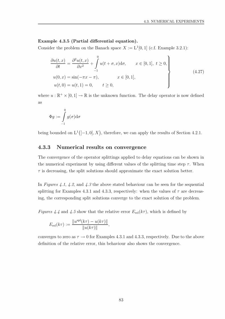
4.3. NUMERICAL EXPERIMENTS
Example 4.3.5 (Partial differential equation).
Consider the problem on the Banach space X := L1[0, 1] (c.f. Example 3.2.1):
∂u(t, x)
∂t=
∂2u(t, x)
∂x2+
0∫
−1
u(t + σ, x)dσ, x ∈ [0, 1], t ≥ 0,
u(0, x) = sin(−πx − π), x ∈ [0, 1],
u(t, 0) = u(t, 1) = 0, t ≥ 0,
(4.27)
where u : R+ × [0, 1] → R is the unknown function. The delay operator is now defined
as
Φg :=
0∫
−1
g(σ)dσ
being bounded on L1([−1, 0], X
), therefore, we can apply the results of Section 4.2.1.
4.3.3 Numerical results on convergence
The convergence of the operator splittings applied to delay equations can be shown in
the numerical experiment by using different values of the splitting time step τ . When
τ is decreasing, the split solutions should approximate the exact solution better.
In Figures 4.1, 4.2, and 4.3 the above stated behaviour can be seen for the sequential
splitting for Examples 4.3.1 and 4.3.3, respectively: when the values of τ are decreas-
ing, the corresponding split solutions converge to the exact solution of the problem.
Figures 4.4 and 4.5 show that the relative error Erel(kτ), which is defined by
Erel(kτ) :=‖uspl(kτ) − u(kτ)‖
‖u(kτ)‖ ,
converges to zero as τ → 0 for Examples 4.3.1 and 4.3.3, respectively. Due to the above
definition of the relative error, this behaviour also shows the convergence.
83
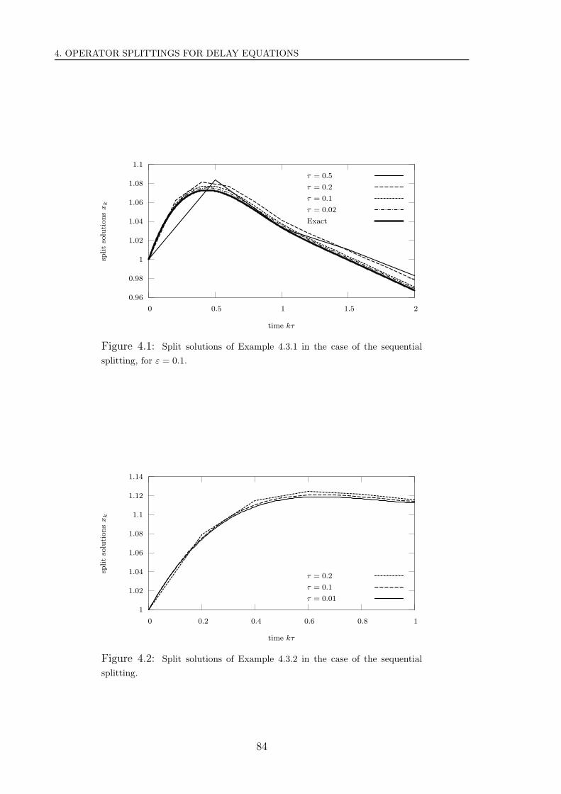
4. OPERATOR SPLITTINGS FOR DELAY EQUATIONS
0.96
0.98
1
1.02
1.04
1.06
1.08
1.1
0 0.5 1 1.5 2
split
solu
tions
xk
time kτ
τ = 0.5
τ = 0.2
τ = 0.1
τ = 0.02
Exact
Figure 4.1: Split solutions of Example 4.3.1 in the case of the sequential
splitting, for ε = 0.1.
1
1.02
1.04
1.06
1.08
1.1
1.12
1.14
0 0.2 0.4 0.6 0.8 1
split
solu
tions
xk
time kτ
τ = 0.2
τ = 0.1
τ = 0.01
Figure 4.2: Split solutions of Example 4.3.2 in the case of the sequential
splitting.
84
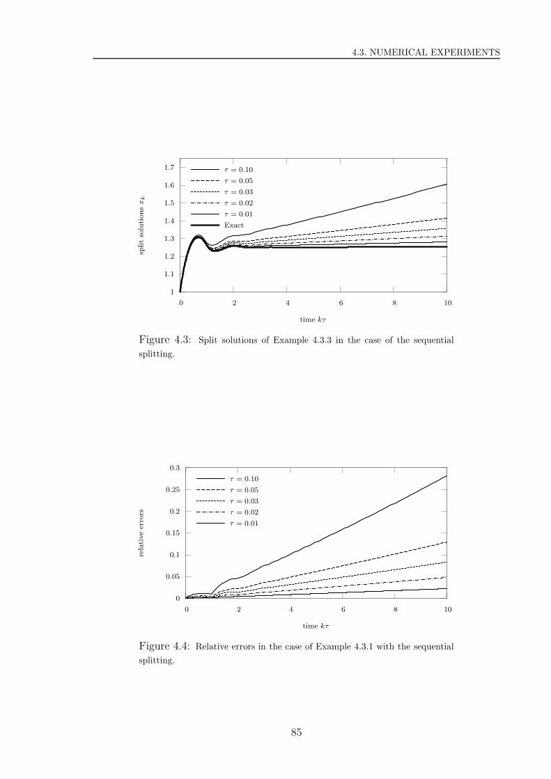
4.3. NUMERICAL EXPERIMENTS
1
1.1
1.2
1.3
1.4
1.5
1.6
1.7
0 2 4 6 8 10
split
solu
tions
xk
time kτ
τ = 0.10
τ = 0.05
τ = 0.03
τ = 0.02
τ = 0.01
Exact
Figure 4.3: Split solutions of Example 4.3.3 in the case of the sequential
splitting.
0
0.05
0.1
0.15
0.2
0.25
0.3
0 2 4 6 8 10
rela
tive
erro
rs
time kτ
τ = 0.10
τ = 0.05
τ = 0.03
τ = 0.02
τ = 0.01
Figure 4.4: Relative errors in the case of Example 4.3.1 with the sequential
splitting.
85
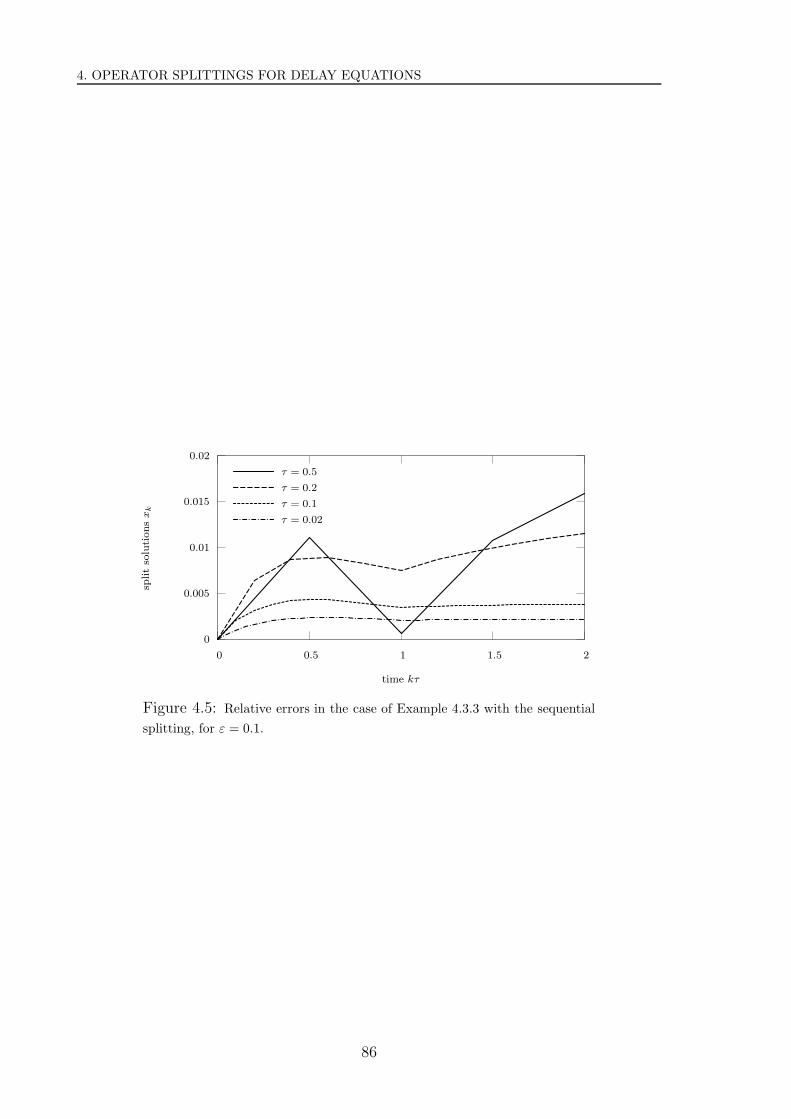
4. OPERATOR SPLITTINGS FOR DELAY EQUATIONS
0
0.005
0.01
0.015
0.02
0 0.5 1 1.5 2
split
solu
tions
xk
time kτ
τ = 0.5
τ = 0.2
τ = 0.1
τ = 0.02
Figure 4.5: Relative errors in the case of Example 4.3.3 with the sequential
splitting, for ε = 0.1.
86
Chapter 5
Error analysis of the solution of
split differential equations
Operator splitting means that the spatial differential operator appearing in the equa-
tions is split into a sum of different sub-operators having simpler forms, and the cor-
responding equations can be solved easier. The sub-operators usually correspond to
the different physical processes or geometric directions. Then instead of the original
problem, a sequence of sub-models is solved (e.g. as in (2.5)), which gives rise to the
splitting error (c.f. Definition 2.2.1). The order of the splitting error can be estimated
theoretically (e.g., Farago and Havasi [28]), however, in practice, splitting procedures
are associated with different numerical methods for solving the sub-problems, which
also cause a certain amount of error. This can usually lead to the interaction between
the two types of errors: the splitting error and the numerical error. Since the orders
of the applied splitting procedure and the numerical method are known, the question
is which order their common effect cause. Therefore, the interaction can be measured
through estimating the order of the total time-discretization method (which means the
application of the splitting and the numerical method together for solving the equation
numerically). If the numerical method is not properly chosen for the applied splitting
procedure then this can lead to order reduction, therefore, loss of accuracy. Moreover,
the choices of the step size of the numerical method and the time parameter of the
splitting procedure play an important role, too.
In this chapter our aim is to analyze the behaviour of the different errors appearing in
the solution. We investigate whether the total error of this method is really the sum
of the numerical and the splitting errors. In practice, only the order of the splitting is
taken into account when considering the accuracy (the order of the numerical method
87

5. ERROR ANALYSIS OF THE SOLUTION OF SPLIT DIFFERENTIAL EQUATIONS
is usually not taken into consideration). This means that the order of the total error
is considered to be equal to the order of the applied splitting procedure. Therefore,
we investigate the conditions under which this consideration really fulfills. We are also
going to find a quantity which characterizes well the accuracy of the method, without
knowing the exact solution.
In the operator splitting community it is well known that there is a kind of order reduc-
tion when applying lower order numerical method than splitting procedure, however,
this statement has never been examined thorougly. This chapter represents a first step
towards the systematic survey of the phenomenon, using simple mathematical and nu-
merical tools (see Csomos and Farago [15] and Csomos [9] and [11]).
5.1 Illustration
In what follows we illustrate the interaction between the splitting procedure and the
numerical method on a simple problem applying sequential splitting (defined in Chap-
ter 2 in (2.5)) and explicit Euler method.
Let (x(t), y(t))T denote a function of type R → R2, and 0 ≤ t ≤ T . The time-evolution
of the harmonic oscillator is described by the following equation (see e.g., Landau and
Lifschitz [47]):
x(t) = y(t)
y(t) = −x(t),t ∈ [0, T ] (5.1)
with x(0) = x0 ∈ R and y(0) = y0 ∈ R. The exact solution of the system (5.1) reads
x(t) = y0 sin t + x0 cos t
y(t) = y0 cos t − x0 sin t(5.2)
where x(t) and y(t) represent the amplitude and the velocity of the oscillator, respec-
tively. The simplest example of an oscillating system is a mass connected to a rigid
foundation with a spring. Equation (5.1) can be written as:
d
dt
(x(t)
y(t)
)=
(0 1
−1 0
)(x(t)
y(t)
). (5.3)
Using the decomposition (splitting) of the matrix appearing in (5.3):(
0 1
−1 0
)=
(1 0
0 1
)+
(−1 1
−1 −1
), (5.4)
88

5.1. ILLUSTRATION
and applying the sequential splitting, the split solution in the points kτ (k = 0, 1, . . . , m)
with τ := Tm
(m ∈ N) has the form:
xspl ((k + 1)τ) = yspl(kτ) sin τ + xspl(kτ) cos τ
yspl ((k + 1)τ) = yspl(kτ) cos τ − xspl(kτ) sin τ,(5.5)
for k = 0, 1, . . . , m, where xspl(0) = x0 and yspl(0) = y0. From (5.2) and (5.5) one can
easily check that
xspl(kτ) = x(kτ)
yspl(kτ) = y(kτ),
for k = 0, 1, . . . , m, thus, splitting does not cause any error in this case.
Let us apply explicit Euler method with step size τ for (5.1). Then the numerical
solution has the form:
xk+1 = xk + τyk
yk+1 = yk − τxk,(5.6)
for k = 0, 1, . . . , m, where x0 = x0 and y0 = y0.
If the explicit Euler method is applied to the split problems, the numerical split solution
has the following form:
xk+1
spl = xkspl + τyk − τ 2
(xk
spl − ykspl
)
yk+1spl = yk
spl − τxk − τ 2(xk
spl + ykspl
),
(5.7)
for k = 0, 1, . . . , m, where x0spl = x0 and y0
spl = y0.
Since the split and the exact solutions do not differ, we are expecting that if we use the
same numerical method for both the split and the unsplit problems, then the numerical
solution and the numerical split solution do not differ, as well. However, comparing
(5.6) and (5.7) one can see that there appears a certain error in the numerical split
solution. Hence, we can see that there is a certain interaction between the splitting
procedure and the numerical method.
In our numerical experiments we used τ = 2π200
while integrating the system (5.1) on the
time interval [0, 4π] with and without applying splitting (the period of the harmonic
oscillator is 2π). On the left panel of Figure 5.1 the effect of the numerical error can
89
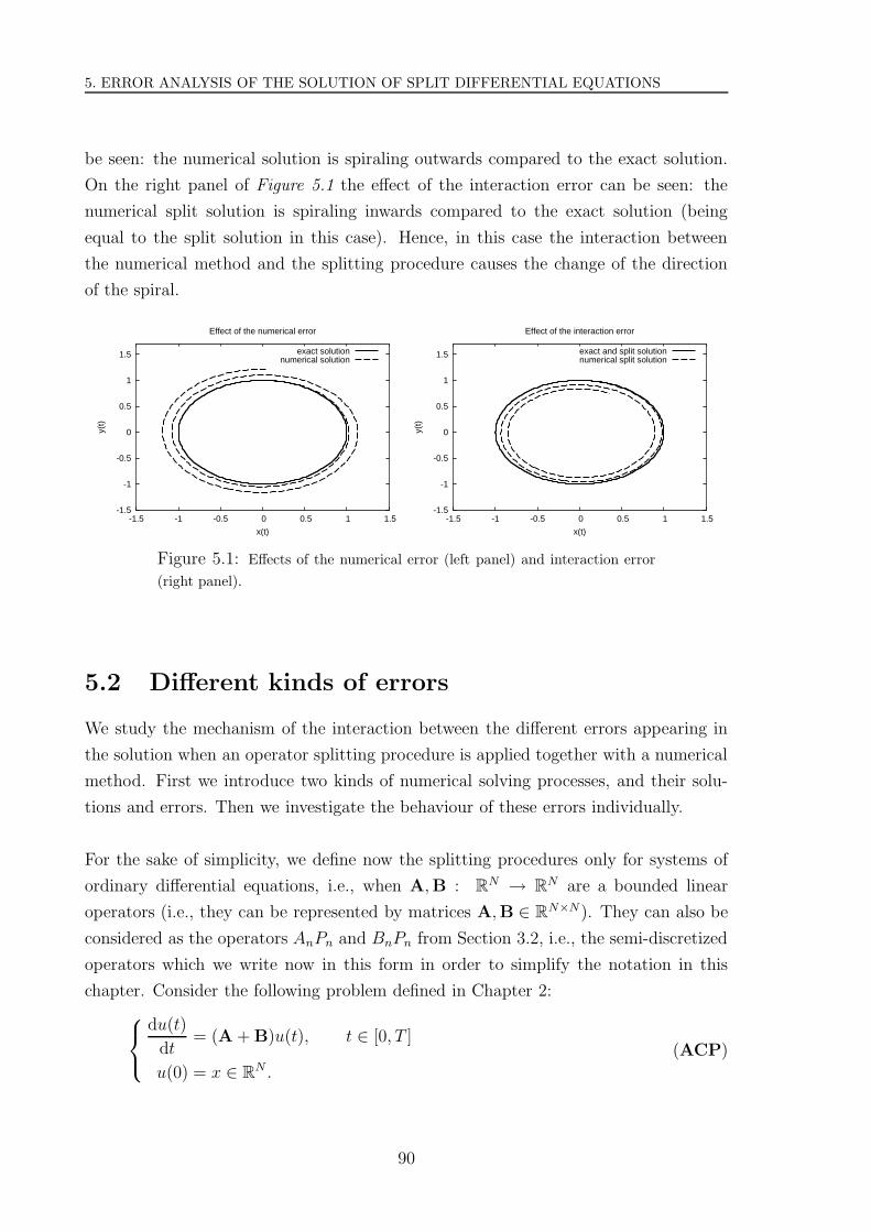
5. ERROR ANALYSIS OF THE SOLUTION OF SPLIT DIFFERENTIAL EQUATIONS
be seen: the numerical solution is spiraling outwards compared to the exact solution.
On the right panel of Figure 5.1 the effect of the interaction error can be seen: the
numerical split solution is spiraling inwards compared to the exact solution (being
equal to the split solution in this case). Hence, in this case the interaction between
the numerical method and the splitting procedure causes the change of the direction
of the spiral.
-1.5
-1
-0.5
0
0.5
1
1.5
-1.5 -1 -0.5 0 0.5 1 1.5
y(t)
x(t)
Effect of the numerical error
exact solutionnumerical solution
-1.5
-1
-0.5
0
0.5
1
1.5
-1.5 -1 -0.5 0 0.5 1 1.5
y(t)
x(t)
Effect of the interaction error
exact and split solutionnumerical split solution
Figure 5.1: Effects of the numerical error (left panel) and interaction error
(right panel).
5.2 Different kinds of errors
We study the mechanism of the interaction between the different errors appearing in
the solution when an operator splitting procedure is applied together with a numerical
method. First we introduce two kinds of numerical solving processes, and their solu-
tions and errors. Then we investigate the behaviour of these errors individually.
For the sake of simplicity, we define now the splitting procedures only for systems of
ordinary differential equations, i.e., when A,B : RN → RN are a bounded linear
operators (i.e., they can be represented by matrices A,B ∈ RN×N). They can also be
considered as the operators AnPn and BnPn from Section 3.2, i.e., the semi-discretized
operators which we write now in this form in order to simplify the notation in this
chapter. Consider the following problem defined in Chapter 2:
du(t)
dt= (A + B)u(t), t ∈ [0, T ]
u(0) = x ∈ RN .
(ACP)
90

5.2. DIFFERENT KINDS OF ERRORS
Then let us apply the sequential, Strang, and weighted splitting procedures defined
in (2.2)–(2.3), (2.6)–(2.8), and (2.11), respectively. We note that our results can be
generalized to more than two sub-operators, as well.
5.2.1 Discretization of the time-continuous problem
Discretization means that the time-continuous problem defined on the interval [0, T ]
is somehow replaced by a sequence of finite dimensional problems. In the case of the
present investigations we used finite difference methods (defined in Section 1.2). Let
us introduce two uniform meshes on [0, T ]:
ωτ := kτ, k = 0, 1, . . . , m and ωh := kh, k = 0, 1, . . . , mn,
where τ = Tm
is the splitting time step defined in Chapter 2 and h = τn
is called the step
size of the numerical method. Throughtout this chapter we will use these notations.
Clearly, ωτ ⊂ ωh. The structures of these meshes are shown in Figure 5.2.
h hh h h...
...τ τ τ
0 Τ...... ...
Figure 5.2: Meshes ωτ and ωh on the interval [0, T ]: τ = Tm
is the splitting
time step, and h = τn
is the step size of the numerical method.
The numerical split solution will only be defined on ωτ . (The numerical solution of the
original problem is defined on ωh but it can only be compared with the split solution
on ωτ .) If n = 1 then ωτ = ωh. Let Xωτdenote the set of the time-discretized functions
mapping ωτ → RN with some vector norm ‖.‖. Our aim is to determine a suitable
solution to (ACP) (from Xωτ). Thus, an element of RN has to be assigned to each
point of ωτ . This can be done in several ways, for instance:
(1) We apply a numerical method directly on the mesh ωh ⊃ ωτ .
(2) First we apply a splitting procedure, and then the split sub-problems are solved
by a certain numerical method. (In this case the sub-problems are solved on the
finer mesh ωh, but the solution is defined on ωτ .)
91
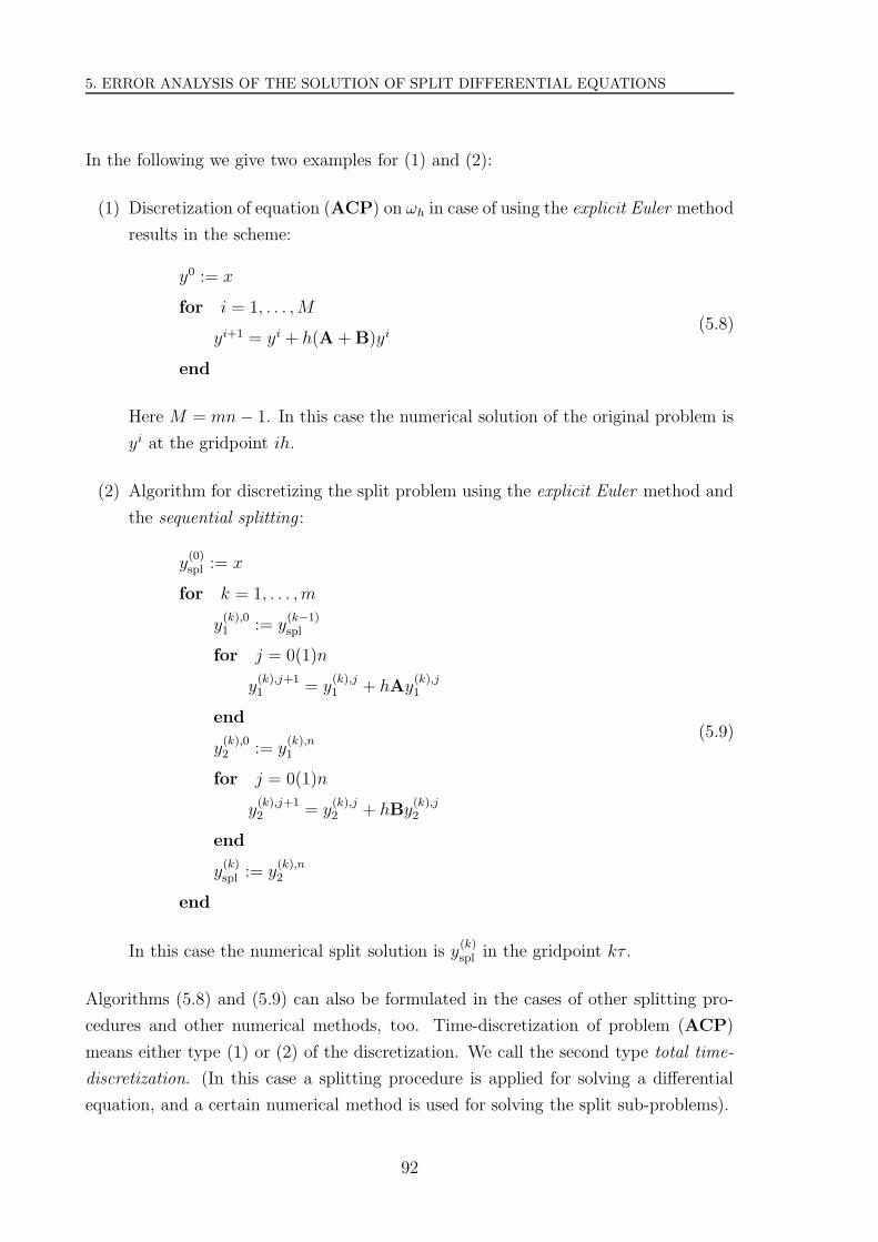
5. ERROR ANALYSIS OF THE SOLUTION OF SPLIT DIFFERENTIAL EQUATIONS
In the following we give two examples for (1) and (2):
(1) Discretization of equation (ACP) on ωh in case of using the explicit Euler method
results in the scheme:
y0 := x
for i = 1, . . . , M
yi+1 = yi + h(A + B)yi
end
(5.8)
Here M = mn − 1. In this case the numerical solution of the original problem is
yi at the gridpoint ih.
(2) Algorithm for discretizing the split problem using the explicit Euler method and
the sequential splitting :
y(0)spl := x
for k = 1, . . . , m
y(k),01 := y
(k−1)spl
for j = 0(1)n
y(k),j+11 = y
(k),j1 + hAy
(k),j1
end
y(k),02 := y
(k),n1
for j = 0(1)n
y(k),j+12 = y
(k),j2 + hBy
(k),j2
end
y(k)spl := y
(k),n2
end
(5.9)
In this case the numerical split solution is y(k)spl in the gridpoint kτ .
Algorithms (5.8) and (5.9) can also be formulated in the cases of other splitting pro-
cedures and other numerical methods, too. Time-discretization of problem (ACP)
means either type (1) or (2) of the discretization. We call the second type total time-
discretization. (In this case a splitting procedure is applied for solving a differential
equation, and a certain numerical method is used for solving the split sub-problems).
92
5.2. DIFFERENT KINDS OF ERRORS
5.2.2 Errors appearing in the numerical solution
Before defining the different kinds of errors being investigated, we introduce four kinds
of solutions (as before, τ is the splitting time step, and h ≤ τ denotes the numerical
step size, m, n ∈ N):
– u(t) denotes the exact solution of the original continuous problem (ACP) at time
t;
– uspl(kτ), k = 1, . . . , m denotes the exact solution of the continuous split problem
(e.g. (2.2)–(2.2)) at time t = kτ , i.e., the split solution;
– ykspl, k = 1, . . . , m denotes the numerical solution of the split problem (e.g. (5.9))
at time t = kτ , i.e.the numerical split solution,
and
– yknum, k = 1, . . . , mn denotes the numerical solution of the original problem
(e.g. (5.8)) at time t = kh.
Definition 5.2.1. Using the above notions for the different solutions, we define the
following four kinds of errors:
total error : Etot(kτ) :=∥∥u(kτ) − yk
spl
∥∥ ;
splitting error : Espl(kτ) := ‖u(kτ) − uspl(kτ)‖ ;
practical error : Eprac(kτ) :=∥∥yk
num − ykspl
∥∥ ;
interaction error : Eint(kτ) :=∥∥uspl(kτ) − yk
spl
∥∥ ,
where k = 1, . . . , m. Let E(kτ) denote any of the above errors. Then E(τ) and
E(mτ) = E(T ) are called local and global errors, respectively. The numerical error can
be defined on the finer mesh ωh:
numerical error : Enum(kh) :=∥∥u(kh) − yk
num
∥∥
for k = 1, . . . , mn, where Enum(h) is the local numerical error, which is raised by the
numerical method.
We remark that in practice, we are interested in Etot(kτ). However, the exact solu-
tion is not known, therefore, we are only be able to measure Eprac(kτ). Hence, we
investigate whether it is possible to estimate Etot(kτ) from Eprac(kτ), i.e., whether
the order of Etot(kτ) follows from the order of Eprac(kτ). It will be shown that the
93
5. ERROR ANALYSIS OF THE SOLUTION OF SPLIT DIFFERENTIAL EQUATIONS
interaction error causes a reduction of the order of the total time-discretization method.
Similarly to Definition 2.2.1 of the order of the local splitting error, we define the orders
of the other errors.
Definition 5.2.2. The local error E(τ) is of order p if
p := sup
q ∈ N : lim
τ→0
E(τ)
τ q+1< +∞
. (5.10)
The operator splitting procedure is called consistent if p ≥ 1 for Espl(τ). The total
time-discretization method is called consistent if p ≥ 1 for Etot(τ).
We note that if the local error E(τ) is of order p (i.e., E(τ) = O(τ p+1)), then the
local error behaves as E(τ) = const · τ p+1 for sufficiently small values of τ . When the
sub-operators are non-stiff, then we may assume that their norms are bounded with
moderate constants, therefore, for the global error we obtain that
E(T ) = mO(τ p+1) =T
τO(τ p+1) = O(τ p).
This means that the order of the global error can be computed from the local error
(c.f. Corollary 1.2.13). For the stiff-case see Sportisse [57].
5.2.3 Local splitting, numerical, and interaction errors
In Section 2.2 we have already derived the order of the sequential splitting as an
example. We recall the orders of the defined splitting procedures presented in Table
2.1 (see Farago and Havasi [28], Hundsdorfer and Verwer [36], Csomos et al. [13]). We
note that the condition on the higher order symmetrically weighted splitting reads as
[[A,B],A− B] = 0. (5.11)
The error Enum(h) represents the local numerical error of the applied numerical method
of order r, therefore, Enum(h) = O(hr+1). When h = τn
and τ are connected with the
relation h = τ s (s = 1, 2, 3, . . . ), then
Enum(h) = O(τ rs+s). (5.12)
Then Enum(τ) represents the global numerical error at time t = τ . Its order can be
estimated as follows:
Enum(τ) = nO(hr+1) =τ
hO(hr+1) = τO(hr) = τO(τ rs) = O(τ rs+1). (5.13)
94
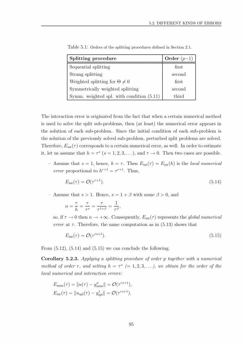
5.2. DIFFERENT KINDS OF ERRORS
Table 5.1: Orders of the splitting procedures defined in Section 2.1.
Splitting procedure Order (p−1)
Sequential splitting first
Strang splitting second
Weighted splitting for Θ 6= 0 first
Symmetrically weighted splitting second
Symm. weighted spl. with condition (5.11) third
The interaction error is originated from the fact that when a certain numerical method
is used to solve the split sub-problems, then (at least) the numerical error appears in
the solution of each sub-problem. Since the initial condition of each sub-problem is
the solution of the previously solved sub-problem, perturbed split problems are solved.
Therefore, Eint(τ) corresponds to a certain numerical error, as well. In order to estimate
it, let us assume that h = τ s (s = 1, 2, 3, . . . ), and τ → 0. Then two cases are possible.
– Assume that s = 1, hence, h = τ . Then Eint(τ) = Eint(h) is the local numerical
error proportional to hr+1 = τ r+1. Thus,
Eint(τ) = O(τ r+1). (5.14)
– Assume that s > 1. Hence, s = 1 + β with some β > 0, and
n =τ
h=
τ
τ s=
τ
τ 1+β=
1
τβ,
so, if τ → 0 then n → +∞. Consequently, Eint(τ) represents the global numerical
error at τ . Therefore, the same computation as in (5.13) shows that
Eint(τ) = O(τ rs+1). (5.15)
From (5.12), (5.14) and (5.15) we can conclude the following.
Corollary 5.2.3. Applying a splitting procedure of order p together with a numerical
method of order r, and setting h = τ s (= 1, 2, 3, . . . ), we obtain for the order of the
local numerical and interaction errors:
Enum(τ) = ‖u(τ) − ynnum‖ = O(τ rs+1),
Eint(τ) = ‖uspl(τ) − y1spl‖ = O(τ rs+1).
95

5. ERROR ANALYSIS OF THE SOLUTION OF SPLIT DIFFERENTIAL EQUATIONS
5.2.4 Local total error
From now on we denote by % the order of the local total error, i.e., Etot(τ) = O(τ %+1).
Applying a splitting procedure of order p together with a numerical method of order r
and using the triangular inequality, we can deduce from Definition 5.2.1 that
Etot(τ) = ‖u(τ) − y1spl‖ ≤ ‖u(τ) − uspl(τ)‖ + ‖uspl(τ) − y1
spl‖ = (5.16)
= Espl(τ) + Eint(τ).
Hence, the local total error can be estimated by the sum of the local splitting error
and the interaction error. From the definition of the order of the local splitting error
and Corollary 5.2.3, from (5.16) we can conclude the following.
Proposition 5.2.4. Let us apply an operator splitting procedure of order p together
with a numerical method of order r, and set h = τ s (= 1, 2, 3, . . . ). Then the order of
the local total error is: % = minp, rs.
This means that in order to preserve the accuracy, we can control it through the pa-
rameters p, r, and s for a given p. In practice, we apply a given splitting procedure,
hence, p and τ are fixed, and we want to preserve the order p to the local total error
(% = p).
From Proposition 5.2.4 it follows that the interaction error causes a decrease in the
order of Etot(τ) unless rs ≥ p.
Corollary 5.2.5. Proposition 5.2.4 implies that % = p if rs ≥ p.
Therefore, we shall answer the following two questions for given values of p and τ .
(i) How to choose h for a given numerical method of order r?
(ii) Fixing h = τ , how to choose the order r of the numerical method?
From Proposition 5.2.4, the following answers can be stated.
Proposition 5.2.6. When a given splitting procedure of order p is applied together
with a given numerical method of order r ≤ p, and the numerical step size is set as
h = τ s, then the exponent s has to be chosen as s = pr
in order to keep % = p. For
r > p the identity % = p holds independently of the choice of h.
Remark 5.2.7. For the case r > p, clearly, the choice h = τ is optimal, because in
this case the integration of the model’s equation needs the least step, hence, the least
computational work.
96
5.3. ANALYTICAL COMPUTATIONS
Proposition 5.2.8. When a given splitting procedure of order p is applied together
with a certain numerical method of order r, and the numerical step size is varied as
h = τ s (= 1, 2, 3, . . . ), then r has to be chosen as r =[
ps
]+ 1 ∈ N in order to keep
% = p.
Remark 5.2.9. Higher order numerical methods could be chosen, as well, but it would
not lead to a higher order total time-discretization. It would only need more computa-
tional work.
5.2.5 Local practical error
If the exact solution is not known, the order of Etot(τ) cannot be derived, hence, we
can only compute the local practical error Eprac(τ). We shall investigate whether the
order of Eprac(τ) differs from the order of Etot(τ). Using the definitions of the local
errors, and the triangular inequality, we get:
|Eprac(τ) − Etot(τ)| =∣∣‖yn
num − y1spl‖ − ‖y1
spl − u(τ)‖∣∣ ≤
≤‖u(τ) − ynnum‖ = Enum(τ).
From Corollary 5.2.3 we obtain that
|Eprac(τ) − Etot(τ)| = O(τ rs+1).
Corollary 5.2.10. Eprac(τ) and Etot(τ) only differ in the order of the global numerical
error. This means that we can characterize the accuracy of the total time-discretization
method with the local practical error, as well. It becomes important when the exact
solution is not known.
5.3 Analytical computations
In this section we investigate the behaviour of the previously studied errors. As before,
we only consider bounded operators, because the semi-discretization always leads to
a system of ordinary differential equations with matrix operators. We remark that
the exponential of a bounded linear operator A can be defined as (see e.g. Def. 2.2 in
Chapter I. of Engel and Nagel [22], c.f. Remark 1.1.22):
exp(A) :=∞∑
k=0
Ak
k!. (5.17)
We note that the original and the split problems are solved by using the same numerical
method.
97

5. ERROR ANALYSIS OF THE SOLUTION OF SPLIT DIFFERENTIAL EQUATIONS
5.3.1 Expressions of the solutions
In order to demonstrate the effect of the interaction error, we compute the expressions
of the exact, the numerical, and the numerical split solutions of (ACP) up to O(τ 3),
using the explicit and implicit Euler method.
The exact solution of the original problem (ACP) and the split solutions obtained by
the different splitting procedures, can be written in the following way for the initial
value x ∈ RN :
Exact solution: u(τ) = exp [τ(A + B)] x
Sequential splitting: usqspl(τ) = exp(τB) exp(τA)x
Strang splitting: uStspl(τ) = exp
(τ2A)exp(τB) exp
(τ2A)x
Weighted splitting: uΘspl(τ) = [Θ exp(τB) exp(τA)
+(1 − Θ) exp(τA) exp(τB)] x. (5.18)
Applying the explicit Euler method with time step h, the numerical and numerical
split solutions can be written in the following form (using the notation yspl := y1spl):
Numerical solution: ynnum = [I + h(A + B)]n x
Sequential sp.: ysqspl = (I + hB)n(I + hA)nx
Strang splitting: yStspl = (I + hA)
n2 (I + hB)n (I + hA)
n2 x
Weighted splitting: yΘspl = Θ [(I + hB)n(I + hA)n
+(1 − Θ)(I + hA)n(I + hB)n] x. (5.19)
Applying the implicit Euler method with time step h, the numerical and numerical
split solutions can be written in the following form (using the notation yspl := y1spl):
Numerical solution: ynnum =
[(I − h(A + B))−1]n x
Sequential splitting: ysqspl =
[(I − hB)−1
]n [(I − hA)−1
]nx
Strang splitting: yStspl =
[(I − hA)−1
]n2[(I − hB)−1
]n [(I − hA)−1
]n2 x
Weighted splitting: yΘspl =
Θ[(I − hB)−1
]n [(I − hA)−1
]n
+(1 − Θ)[(I − hA)−1
]n [(I − hB)−1
]nx. (5.20)
After expanding the exponential function in (5.18) into Taylor-series up to O(τ 3), and
using the binomial theorem to expand the other terms in (5.19) and (5.20), the solutions
98

5.3. ANALYTICAL COMPUTATIONS
u(τ), ynnum and yspl can be written as follows:
u(τ)
ynnum
yspl
=
[I + τ(A + B) +
τ 2
2W + O(τ 3)
]x, (5.21)
where the term W has the following meaning in the different cases, using explicit and
implicit Euler methods:
Exact solution (u(τ)): A2 + B2 + AB + BA
Numerical solution (ynnum):
(1 ∓ 1
n
)(A2 + B2) +
(1 ∓ 1
n
)(AB + BA)
Sequential splitting (ysqspl):
(1 ∓ 1
n
)(A2 + B2) + 2BA
Strang splitting (yStspl):
(1 ∓ 1
n
)(A2 + B2) + AB + BA
Weighted splitting (yΘspl):
(1 ∓ 1
n
)(A2 + B2)
+ (1 − Θ)AB + ΘBA, (5.22)
where the upper sign refers to the case of the explicit, and the lower sign to the case
of the implicit Euler method.
Corollary 5.3.1. All of the introduced splitting techniques combined with the Euler
methods are consistent for arbitrary h = τn, because the term I + τ(A + B) in Etot(τ)
vanishes in the difference u(t) − yspl. Hence, p ≥ 1 in Definition 5.2.2.
Remark 5.3.2. We note that from formulae (5.22) one can derive a higher order
time-discretization method, as well. Let the total time-discretization method be chosen
as the average of the terms obtained by using the explicit and implicit Euler methods
in ynnum. Then we get the exact solution up to O(τ 3), therefore, this method is of (at
least) second order.
Remark 5.3.3. We also note that if we average the terms obtained by using the explicit
and implicit Euler methods in the numerical split solutions (ysqspl, ySt
spl, and yΘspl), we get
the formulae of the split solutions up to O(τ 3).
99

5. ERROR ANALYSIS OF THE SOLUTION OF SPLIT DIFFERENTIAL EQUATIONS
5.3.2 Expression of the local errors
From the previously derived formulae (5.18) and (5.22), and taking into account that
h = τn
one can compute the expressions of the local errors up to O(τ 3).
Proposition 5.3.4. From formulae (5.18) and (5.22), simple calculations show the
followings.
Espl(τ) = γ τ2
2(BA− AB) + O(τ 3);
Eint(τ) = χhτ2
(A2 + B2) + O(τ 3);
Etot(τ) =∥∥∥[γ τ2
2(BA− AB) + χhτ
2(A2 + B2)
]x∥∥∥ + O(τ 3) (5.23)
≤ Espl(τ) + Eint(τ) + O(τ 3);
Eprac(τ) =∥∥∥[γ τ2
2(BA + AB) − χhτ
2(A2 + B2)
]x∥∥∥ + O(τ 3),
where χ = 1 and χ = −1 for the explicit and implicit Euler methods, respectively.
The values of γ are: 1, 0, and Θ − 12
for the sequential, the Strang, and the weighted
splittings, respectively.
These results show that estimate (5.16) cannot be sharpened, i.e., the local total error
is less than or equal to the sum of the local splitting and the interaction errors up
to O(τ 3). Furthermore, the step size of the numerical method has to be chosen as
stated in Proposition 5.2.6. For the first-order Euler methods this means that for the
first-order splittings there is no restriction for the numerical step size due to h ≤ τ .
However, in the case of the second-order splittings the numerical step size has to be
chosen as h = O(τ 2) in order to keep the order of the interaction error (i.e., the local
total error) equal to p. The explanation of the observed behaviour is that the explicit
and the implicit Euler methods are of first-order.
One can see that h as well as τ appear in the expression of Eint(τ) in (5.23), thus,
this error is caused by the interaction between the numerical and the splitting errors,
indeed. This is the reason why we call it “interaction error”.
Corollary 5.3.5. Although the local total and practical errors do not have the same
value, their orders equal up to O(τ 3) (c.f. Corollary 5.2.10).
Corollary 5.3.5 implies that for investigating the order of the total time-discretization
method, the local practical error can be computed instead of the local total error. Fi-
nally, we remark that in this section we computed the expressions of the local errors
only up to O(τ 3). We remark that the symmetrically weighted splitting is of third
100

5.4. NUMERICAL EXPERIMENTS
order if the condition (5.11) is satisfied. In this case the step size has to be chosen
at least h = O(τ 2). Based on Proposition 5.2.6 we are expecting, however, that the
suitable choice for the numerical step size should be h = O(τ 3).
5.4 Numerical experiments
We continue our computations related to the order of the local errors by using numerical
simulations. We determine the order of Etot(τ) and Eprac(τ) for a test problem, namely,
for the system of ordinary differential equations corresponding to the model of the
harmonic oscillator.
5.4.1 Test problem
The model of the harmonic oscillator has already been introduced in Section 5.1. We
choose this model because its exact solution is bounded and periodic, therefore, we
can investigate the local errors also for a large range of values of the numerical step
size. We define the following one-parameter splitting family for the matrix appearing
in (5.3):
(0 1
−1 0
)=
(α 0.5
1 0
)+
(−α 0.5
−2 0
), (5.24)
with the parameter α ∈ R. With these sub-matrices, the already mentioned splitting
schemes can be applied: sequential, Strang, weighted, symmetrically weighted (with
α 6= 0, in the numerical experiments α = 0.3), and symmetrically weighted splitting
with condition (5.11) (with α = 0). We used five different numerical methods for
solving the sub-problems: explicit Euler, implicit Euler, second-order midpoint rule,
third- and fourth-order Runge-Kutta method.
5.4.2 Determination of the local orders
Throughout this section E(τ) denotes either Etot(τ) or Eprac(τ). Previously the orders
of E(τ) were computed analytically for the explicit and implicit Euler method up to
O(τ 3). Numerically, they can be determined in two ways. As a first way, the order
of the local errors can be computed as a limit. In the second way, the order can be
determined by fitting a straight line on the numerical data of the function E(τ) in
logarithmic scale.
101

5. ERROR ANALYSIS OF THE SOLUTION OF SPLIT DIFFERENTIAL EQUATIONS
First method
We can apply Definition 5.2.2 of the order, with the difference that q ∈ R. Using the
notation
Hq(τ) :=E(τ)
τ q+1,
the following limit has to be computed numerically for different fixed values of q:
limτ→0
Hq(τ). (5.25)
We note that for a fixed step size h τ , this limit should be understood as τ → h,
therefore, we select h to be close to the computer zero.
Definition 5.4.1. The orders of the local total and practical errors obtained by nu-
merical experiments are called numerical orders of the corresponding local errors, and
they are denoted by %totnum and %prac
num, respectively.
By numerical experiments (with unknown exact solution) we can only determine the
numerical order %pracnum of the total time-discretization method. Therefore, we investigate
the condition for %pracnum = p instead of % = p, where % denotes the “real” order of the
local total error (not its numerical estimate). We assume, however, that %totnum ≈ %, and
we will show that %totnum = %prac
num.
In this case the numerical orders of Etot(τ) and Eprac(τ) are determined as the supre-
mum of those values of q for which the limit in (5.25) is finite. The term Hq(τ) has
been computed for several values of τ and q. In Figure 5.3 the results are shown for
Eprac(τ) applying sequential splitting with the explicit Euler method (with a fixed step
size h = 10−6 τ), for the following 20 values of q: 0.9, 0.91, 0.92,. . . , 1.1. The
splitting time step τ is varied from 2π200
to 2π10
by 2π200
(20 values). We obtained similar
figures also in the case of Etot(τ), and for all kinds of splitting techniques and numerical
methods.
Figure 5.3 shows the validity of the following statement.
Corollary 5.4.2. There exists a threshold q0 such that for q ≤ q0 the function Hq(τ)
is convergent, and for q > q0 it is divergent as τ tends to zero.
The threshold q0 can be considered as the numerical order of the total time-discretization
method (Etot(τ) or Eprac(τ)), i.e., q0 = %totnum or q0 = %prac
num. According to the orders
of the splitting procedure and the numerical method, different values of q0 belong to
102
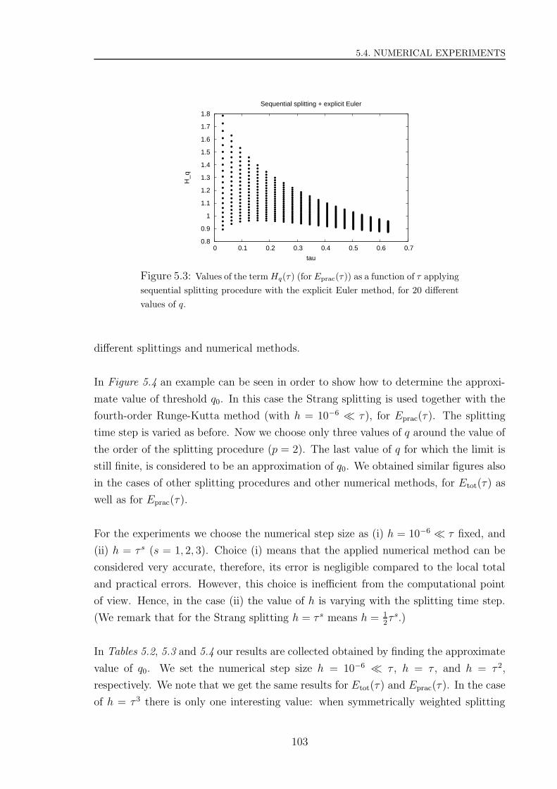
5.4. NUMERICAL EXPERIMENTS
0.8
0.9
1
1.1
1.2
1.3
1.4
1.5
1.6
1.7
1.8
0 0.1 0.2 0.3 0.4 0.5 0.6 0.7
H_q
tau
Sequential splitting + explicit Euler
Figure 5.3: Values of the term Hq(τ) (for Eprac(τ)) as a function of τ applying
sequential splitting procedure with the explicit Euler method, for 20 different
values of q.
different splittings and numerical methods.
In Figure 5.4 an example can be seen in order to show how to determine the approxi-
mate value of threshold q0. In this case the Strang splitting is used together with the
fourth-order Runge-Kutta method (with h = 10−6 τ), for Eprac(τ). The splitting
time step is varied as before. Now we choose only three values of q around the value of
the order of the splitting procedure (p = 2). The last value of q for which the limit is
still finite, is considered to be an approximation of q0. We obtained similar figures also
in the cases of other splitting procedures and other numerical methods, for Etot(τ) as
well as for Eprac(τ).
For the experiments we choose the numerical step size as (i) h = 10−6 τ fixed, and
(ii) h = τ s (s = 1, 2, 3). Choice (i) means that the applied numerical method can be
considered very accurate, therefore, its error is negligible compared to the local total
and practical errors. However, this choice is inefficient from the computational point
of view. Hence, in the case (ii) the value of h is varying with the splitting time step.
(We remark that for the Strang splitting h = τ s means h = 12τ s.)
In Tables 5.2, 5.3 and 5.4 our results are collected obtained by finding the approximate
value of q0. We set the numerical step size h = 10−6 τ , h = τ , and h = τ 2,
respectively. We note that we get the same results for Etot(τ) and Eprac(τ). In the case
of h = τ 3 there is only one interesting value: when symmetrically weighted splitting
103
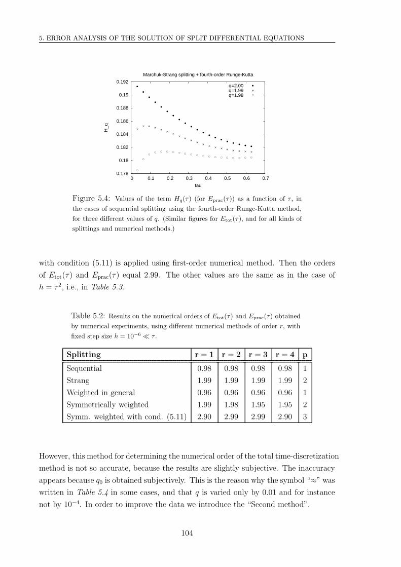
5. ERROR ANALYSIS OF THE SOLUTION OF SPLIT DIFFERENTIAL EQUATIONS
0.178
0.18
0.182
0.184
0.186
0.188
0.19
0.192
0 0.1 0.2 0.3 0.4 0.5 0.6 0.7
H_q
tau
Marchuk-Strang splitting + fourth-order Runge-Kutta
q=2.00q=1.99q=1.98
Figure 5.4: Values of the term Hq(τ) (for Eprac(τ)) as a function of τ , in
the cases of sequential splitting using the fourth-order Runge-Kutta method,
for three different values of q. (Similar figures for Etot(τ), and for all kinds of
splittings and numerical methods.)
with condition (5.11) is applied using first-order numerical method. Then the orders
of Etot(τ) and Eprac(τ) equal 2.99. The other values are the same as in the case of
h = τ 2, i.e., in Table 5.3.
Table 5.2: Results on the numerical orders of Etot(τ) and Eprac(τ) obtained
by numerical experiments, using different numerical methods of order r, with
fixed step size h = 10−6 τ .
Splitting r = 1 r = 2 r = 3 r = 4 p
Sequential 0.98 0.98 0.98 0.98 1
Strang 1.99 1.99 1.99 1.99 2
Weighted in general 0.96 0.96 0.96 0.96 1
Symmetrically weighted 1.99 1.98 1.95 1.95 2
Symm. weighted with cond. (5.11) 2.90 2.99 2.99 2.90 3
However, this method for determining the numerical order of the total time-discretization
method is not so accurate, because the results are slightly subjective. The inaccuracy
appears because q0 is obtained subjectively. This is the reason why the symbol “≈” was
written in Table 5.4 in some cases, and that q is varied only by 0.01 and for instance
not by 10−4. In order to improve the data we introduce the “Second method”.
104
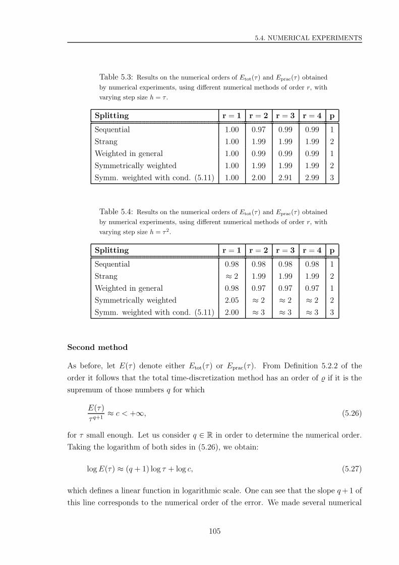
5.4. NUMERICAL EXPERIMENTS
Table 5.3: Results on the numerical orders of Etot(τ) and Eprac(τ) obtained
by numerical experiments, using different numerical methods of order r, with
varying step size h = τ .
Splitting r = 1 r = 2 r = 3 r = 4 p
Sequential 1.00 0.97 0.99 0.99 1
Strang 1.00 1.99 1.99 1.99 2
Weighted in general 1.00 0.99 0.99 0.99 1
Symmetrically weighted 1.00 1.99 1.99 1.99 2
Symm. weighted with cond. (5.11) 1.00 2.00 2.91 2.99 3
Table 5.4: Results on the numerical orders of Etot(τ) and Eprac(τ) obtained
by numerical experiments, using different numerical methods of order r, with
varying step size h = τ2.
Splitting r = 1 r = 2 r = 3 r = 4 p
Sequential 0.98 0.98 0.98 0.98 1
Strang ≈ 2 1.99 1.99 1.99 2
Weighted in general 0.98 0.97 0.97 0.97 1
Symmetrically weighted 2.05 ≈ 2 ≈ 2 ≈ 2 2
Symm. weighted with cond. (5.11) 2.00 ≈ 3 ≈ 3 ≈ 3 3
Second method
As before, let E(τ) denote either Etot(τ) or Eprac(τ). From Definition 5.2.2 of the
order it follows that the total time-discretization method has an order of % if it is the
supremum of those numbers q for which
E(τ)
τ q+1≈ c < +∞, (5.26)
for τ small enough. Let us consider q ∈ R in order to determine the numerical order.
Taking the logarithm of both sides in (5.26), we obtain:
log E(τ) ≈ (q + 1) log τ + log c, (5.27)
which defines a linear function in logarithmic scale. One can see that the slope q +1 of
this line corresponds to the numerical order of the error. We made several numerical
105
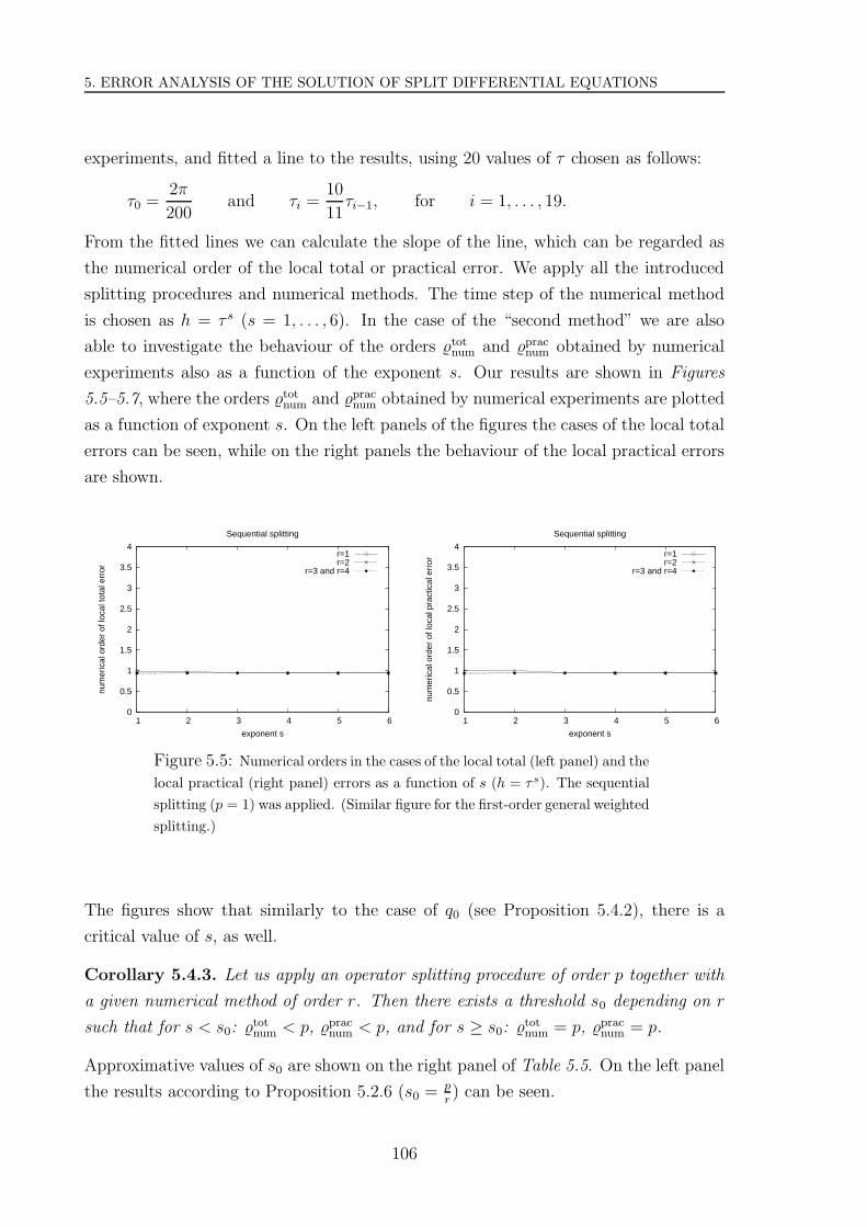
5. ERROR ANALYSIS OF THE SOLUTION OF SPLIT DIFFERENTIAL EQUATIONS
experiments, and fitted a line to the results, using 20 values of τ chosen as follows:
τ0 =2π
200and τi =
10
11τi−1, for i = 1, . . . , 19.
From the fitted lines we can calculate the slope of the line, which can be regarded as
the numerical order of the local total or practical error. We apply all the introduced
splitting procedures and numerical methods. The time step of the numerical method
is chosen as h = τ s (s = 1, . . . , 6). In the case of the “second method” we are also
able to investigate the behaviour of the orders %totnum and %prac
num obtained by numerical
experiments also as a function of the exponent s. Our results are shown in Figures
5.5–5.7, where the orders %totnum and %prac
num obtained by numerical experiments are plotted
as a function of exponent s. On the left panels of the figures the cases of the local total
errors can be seen, while on the right panels the behaviour of the local practical errors
are shown.
0
0.5
1
1.5
2
2.5
3
3.5
4
1 2 3 4 5 6
num
eric
al o
rder
of l
ocal
tota
l err
or
exponent s
Sequential splitting
r=1r=2
r=3 and r=4
0
0.5
1
1.5
2
2.5
3
3.5
4
1 2 3 4 5 6
num
eric
al o
rder
of l
ocal
pra
ctic
al e
rror
exponent s
Sequential splitting
r=1r=2
r=3 and r=4
Figure 5.5: Numerical orders in the cases of the local total (left panel) and the
local practical (right panel) errors as a function of s (h = τ s). The sequential
splitting (p = 1) was applied. (Similar figure for the first-order general weighted
splitting.)
The figures show that similarly to the case of q0 (see Proposition 5.4.2), there is a
critical value of s, as well.
Corollary 5.4.3. Let us apply an operator splitting procedure of order p together with
a given numerical method of order r. Then there exists a threshold s0 depending on r
such that for s < s0: %totnum < p, %prac
num < p, and for s ≥ s0: %totnum = p, %prac
num = p.
Approximative values of s0 are shown on the right panel of Table 5.5. On the left panel
the results according to Proposition 5.2.6 (s0 = pr) can be seen.
106
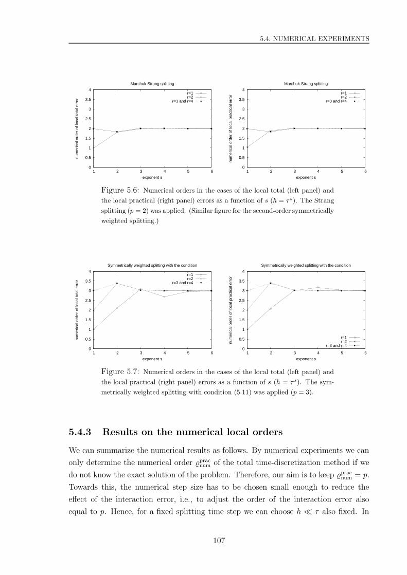
5.4. NUMERICAL EXPERIMENTS
0
0.5
1
1.5
2
2.5
3
3.5
4
1 2 3 4 5 6
num
eric
al o
rder
of l
ocal
tota
l err
or
exponent s
Marchuk-Strang splitting
r=1r=2
r=3 and r=4
0
0.5
1
1.5
2
2.5
3
3.5
4
1 2 3 4 5 6
num
eric
al o
rder
of l
ocal
pra
ctic
al e
rror
exponent s
Marchuk-Strang splitting
r=1r=2
r=3 and r=4
Figure 5.6: Numerical orders in the cases of the local total (left panel) and
the local practical (right panel) errors as a function of s (h = τ s). The Strang
splitting (p = 2) was applied. (Similar figure for the second-order symmetrically
weighted splitting.)
0
0.5
1
1.5
2
2.5
3
3.5
4
1 2 3 4 5 6
num
eric
al o
rder
of l
ocal
tota
l err
or
exponent s
Symmetrically weighted splitting with the condition
r=1r=2
r=3 and r=4
0
0.5
1
1.5
2
2.5
3
3.5
4
1 2 3 4 5 6
num
eric
al o
rder
of l
ocal
pra
ctic
al e
rror
exponent s
Symmetrically weighted splitting with the condition
r=1r=2
r=3 and r=4
Figure 5.7: Numerical orders in the cases of the local total (left panel) and
the local practical (right panel) errors as a function of s (h = τ s). The sym-
metrically weighted splitting with condition (5.11) was applied (p = 3).
5.4.3 Results on the numerical local orders
We can summarize the numerical results as follows. By numerical experiments we can
only determine the numerical order %pracnum of the total time-discretization method if we
do not know the exact solution of the problem. Therefore, our aim is to keep %pracnum = p.
Towards this, the numerical step size has to be chosen small enough to reduce the
effect of the interaction error, i.e., to adjust the order of the interaction error also
equal to p. Hence, for a fixed splitting time step we can choose h τ also fixed. In
107
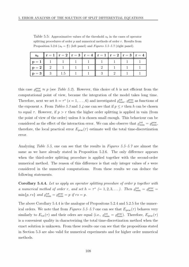
5. ERROR ANALYSIS OF THE SOLUTION OF SPLIT DIFFERENTIAL EQUATIONS
Table 5.5: Approximative values of the threshold s0 in the cases of operator
splitting procedures of order p and numerical methods of order r. Results from
Proposition 5.2.6 (s0 = p
r) (left panel) and Figures 5.5–5.7 (right panel).
s0 r = 1 r = 2 r = 3 r = 4 r = 1 r = 2 r = 3 r = 4
p = 1 1 1 1 1 1 1 1 1
p = 2 2 1 1 1 2 1 1 1
p = 3 3 1.5 1 1 3 2 1 1
this case %pracnum ≈ p (see Table 5.2). However, this choice of h is not efficient from the
computational point of view, because the integration of the model takes long time.
Therefore, next we set h = τ s (s = 1, . . . , 6) and investigated %totnum, %prac
num as functions of
the exponent s. From Tables 5.3 and 5.4 one can see that if p ≤ r then h can be chosen
to equal τ . However, if p > r then the higher order splitting is applied in vain (from
the point of view of the order) unless h is chosen small enough. This behaviour can be
considered as the effect of the interaction error. We can also observe that %totnum = %prac
num,
therefore, the local practical error Eprac(τ) estimate well the total time-discretization
error.
Analyzing Table 5.5, one can see that the results in Figures 5.5–5.7 are almost the
same as we have already stated in Proposition 5.2.6. The only difference appears
when the third-order splitting procedure is applied together with the second-order
numerical method. The reason of this difference is that only integer values of s were
considered in the numerical computations. From these results we can deduce the
following statements.
Corollary 5.4.4. Let us apply an operator splitting procedure of order p together with
a numerical method of order r, and set h = τ s (= 1, 2, 3, . . . ). Then %totnum = %prac
num =
minp, rs and %totnum = %prac
num = p if rs = p.
The above Corollary 5.4.4 is the analogue of Propositons 5.2.4 and 5.2.5 for the numer-
ical orders. We note that from Figures 5.5–5.7 one can see that Eprac(τ) behaves very
similarly to Etot(τ) and their oders are equal (i.e., %totnum = %prac
num). Therefore, Eprac(τ)
is a convenient quality in characterizing the total time-discretization method when the
exact solution is unknown. From these results one can see that the propositions stated
in Section 5.3 are also valid for numerical experiments and for higher order numerical
methods.
108

5.4. NUMERICAL EXPERIMENTS
Summarizing this chapter we can state that the order of the total error is less than the
order of the applied splitting procedure, if the the order of the numerical error and the
numerical time step are not chosen properly.
109

Chapter 6
Analysis of a transport model
applying operator splitting
In Section 1.4 we have introduced the mathematical formulation of the air pollution
transport model (APTM). Due to the complexity of the system (APTM), it may not
be easy to implement a convenient numerical method, which could be efficiently used
to solve the problem. In order to simplify the system, the operator splitting procedure
can be applied. In the model each sub-model describes mathematically one of the phys-
ical processes, i.e., advection, diffusion, emission, deposition, and chemical reactions.
Then instead of one complicated problem more easier sub-problems have to be solved
individually.
When solving numerically the air pollution transport model, two requirements have to
be taken into account: (i) to obtain sufficiently accurate numerical solutions and (ii) to
minimize the computing (or CPU). This means that the error caused by the numerical
solving procedure has to be small, and the numerical solution has to be computed in
a short time. The two above requirements, however, usually contradict each other,
because for small error we would need small time steps, which would cause long CPU
time. In this chapter we present an idea for “resolving” this contradiction by applying
operator splitting (see Csomos [12] and Csomos [10]).
In Chapter 2 we have defined the most important splitting procedures. In this chapter
we will focus on the sequential and the Strang splittings (defined in (2.2)–(2.3) and
(2.6)–(2.8), respectively), because these are usually applied in the air pollution trans-
port models (e.g. in the Danish Eulerian Model, see Zlatev [67], Dimov et al. [21],
Dimov and Zlatev [20], Havasi et al. [34]). We recall that the application of a splitting
111
6. ANALYSIS OF A TRANSPORT MODEL APPLYING OPERATOR SPLITTING
procedure gives rise to the splitting error (see Definition 2.2.1). According to their
accuracy, the sequential splitting is of first order, and the Strang splitting is of second
order. Thus, as a rule, we expect more accurate solution by using the Strang splitting.
As we have already mentioned, we can shorten the integration time needed for solving
the model’s equations with the help of applying operator splitting. As one can see, the
great advantage of applying a splitting procedure is that the sub-problems are solved
individually. Therefore, different spatial and time discretization methods can be used
for solving each of them. Furthermore, different time steps can be chosen for each
sub-model, as well. In practice, this means that each time step (for fixed grid sizes)
can be chosen such that it satisfies the stability condition only of the corresponding
discretization method. The only important restriction is that the solutions have to be
evaluated at the splitting time steps, i.e., in times kτ (k = 1, . . . , m). If we do not
apply any splitting procedure, the numerical time step should be chosen satisfying the
most severe stability condition of the sub-models (which results in the shortest time
step). Therefore, an advantage of applying a splitting technique is that the calculations
need less CPU time than without applying any splitting procedure. In what follows we
justify this idea in the case of the air pollution model. We compare the solutions and
the CPU times obtained (i) without applying splitting, and (ii) by applying splitting
together with two different schemes for solving the advection sub-model: the upwind
scheme (with small time step) and the semi-Lagrangian schemes (with larger time
step).
6.1 Setting of the test model
In our test model the time-evolution of the concentration of one chemical species is
investigated in two dimensions, without taking into account the effect of chemical
reactions. The forecast domain Ω is defined as follows:
Ω := [0, Xmax] × [0, Ymax].
Thus, as a special case of the air pollution model (APTM) introduced in Section 1.4,
we consider the following model equation:
∂c
∂t= −
(∂ (uc)
∂x+
∂ (vc)
∂y
)+ K0
(∂2c
∂x2+
∂2c
∂y2
)+ E − σ0c,
c(x, y, 0) = 0
(6.1)
112
6.1. SETTING OF THE TEST MODEL
where (x, y) ∈ Ω and c = c(x, y, t) is the unknown concentration, u = (u(x, y), v(x, y))
is the two dimensional wind velocity field, and K0 = 0.3 km2
h, σ0 = 10−5 1
h. The emission
function E = E(x, y, t) describes a simple physical phenomena: the homogeneous
emission of a circle-shaped industrial area:
E(x, y, t) =
E0, (x − x0)2 + (y − y0)
2 ≤ R2
0, anywhere else,(6.2)
where (x0, y0) and R represent the center and the radius of the area, respectively, and E0
is constant in space and time. For the numerical experiments we choose E0 = 10−4 kgkm3h
and R = 2.5 km. We study the equation (6.1) by using an outflow boundary condition
allowing the polluting material to leave the domain Ω, and we assume no outer sources
of pollution. We use two kinds of wind fields: (i) a constant wind velocity field with
u0 = v0 = 0.2 kmh
, and (ii) the Molenkampf –Crowley advection described by
u(x, y, t) = −%(x − x), v(x, y, t) = %(y − y)
where (x, y) is the center of the advection field. In our numerical experiments we
choose % = 0.01 1h, and x = 10 km, y = 10 km for constant wind velocity, and
x = 40 km, y = 10 km for the Molenkampf –Crowley advection. In Figure 6.1 the
effect of the Molenkampf –Crowley advection is shown: it rotates the pollution around
the center of the domain (here x = y = 100 km). One can observe the effect of the
diffusion as well: the path of the pollution becomes wider farther from the emission.
We consider the following sub-operators in the splitting procedures (2.2)–(2.3) and
(2.6)–(2.8) defined in Chapter 2:
A := K0
(∂2c
∂x2+
∂2c
∂y2
)+ E − σ0c, (6.3)
B := −(
∂ (uc)
∂x+
∂ (vc)
∂y
),
i.e., the first sub-operator describes the effect of the diffusion, the emission, and the
deposition together. The second sub-operator represents the effect of the advection
only. In the numerical experiments we choose the splitting time step τ = 1 hour, the
time step of the numerical method ∆t = 1 minute, and integration time T = 72 hour.
113

6. ANALYSIS OF A TRANSPORT MODEL APPLYING OPERATOR SPLITTING
Figure 6.1: Effect of the Molenkampf –Crowley advection.
6.2 Spatial discretization methods
Since we use finite difference methods for discretizing the equations (see details later),
we introduce the following mesh:
Ω∆ := (i · ∆x, j · ∆y) : i = 0, . . . , I, j = 0, . . . , J ,
where ∆x = Xmax
Iand ∆y = Ymax
Jare the grid sizes of the mesh Ω∆.
In order to realize the outflow boundary condition, we define virtual points around the
mesh Ω∆, and the value of the concentration in these points are computed from second-
order interpolation using three points inside the mesh Ω∆. Then we can compute the
derivatives at the “real” boundary points, as well. In the numerical experiments we
choose Xmax = Ymax = 50 km, ∆x = ∆y = 0.25 km. In the following, we summarise
the discretization methods applied in our air pollution transport model (6.1).
114
6.2. SPATIAL DISCRETIZATION METHODS
6.2.1 Discretization of the diffusion – emission – deposition sub-
model
For discretizing the sub-model with the sub-operator A defined in (6.3), we use the
following explicit finite difference method:
cn+1i,j − cn
i,j
∆t= K0
cni+1,j − 2cn
i,j + cni−1,j
∆x2
+K0
cni,j+1 − 2cn
i,j + cni,j−1
∆y2(6.4)
+ Eni,j − σ0c
ni,j,
where cni,j is the numerical approximation of the concentration at the time n · ∆t and
at the gridpoint (i · ∆x, j · ∆y) ∈ Ω∆, and Eni,j = E(i · ∆x, j · ∆y, n · ∆t), where
n = 0, 1, . . . , T∆t
. One can check that this scheme is stable if the following stability
condition fulfils:
∆t
(1
(∆x)2+
1
(∆y)2
)≤ 1 − σ0
2K0. (6.5)
6.2.2 Discretization of the advection sub-model
For discretizing the sub-model with the sub-operator B defined in (6.3) we use two
different schemes: the upwind and the semi-Lagrangian schemes.
Upwind scheme. When measurements are available in certain temporal and spatial
points, it is useful to discretize the advection sub-model directly on the mesh Ω∆,
applying the upwind scheme, which can be written as:
if uni,j ≥ 0, vn
i,j ≥ 0 :
cn+1i,j − cn
i,j
∆t= −
uni+1,jc
ni+1,j − un
i,jcni,j
∆x−
vni,j+1c
ni,j+1 − vn
i,jcni,j
∆y, (6.6)
if uni,j ≥ 0, vn
i,j < 0 :
cn+1i,j − cn
i,j
∆t= −
uni+1,jc
ni+1,j − un
i,jcni,j
∆x−
vni,jc
ni,j − vn
i,j−1cni,j−1
∆y, (6.7)
if uni,j < 0, vn
i,j ≥ 0 :
cn+1i,j − cn
i,j
∆t= −
uni,jc
ni,j − un
i−1,jcni−1,j
∆x−
vni,j+1c
ni,j+1 − vn
i,jcni,j
∆y, (6.8)
115
6. ANALYSIS OF A TRANSPORT MODEL APPLYING OPERATOR SPLITTING
if uni,j < 0, vn
i,j < 0 :
cn+1i,j − cn
i,j
∆t= −
uni,jc
ni,j − un
i−1,jcni−1,j
∆x−
vni,jc
ni,j − vn
i,j−1cni,j−1
∆y, (6.9)
where cni,j and (un
i,j, vni,j) denote the approximations of c and (u, v), respectively, at time
n · ∆t (n = 0, . . . , T∆t
) at the gridpoint (i · ∆x, j · ∆y) ∈ Ω∆. The scheme (6.6)-(6.9)
is stable only if the Courant – Friedrichs –Levy condition is satisfied (see Courant et
al. [19]), namely,
∆t|vmax|
min∆x, ∆y ≤ 1 (6.10)
where vmax is the maximal wind velocity vector appearing during the integration of
the equation. Hence, applying this scheme with fixed grid sizes ∆x, ∆y, the time step
∆t has to be chosen carefully.
Semi-Lagrangian scheme. The advection sub-model can also be solved from the
point of view of the flowing medium. Then we assume that each fluid domain contains
a certain amount of pollution which is constant during one time step ∆t. When solving
the equation in the semi-Lagrangian aspect, we follow all fluid domains back in time,
and examine their pollution-contents. The same amount of pollution they had at time
t, they should have at time t+∆t. In order to determine the path of each fluid domain,
as a first guess we say that a certain fluid domain comes from the dimensionless distance√
d2x + d2
y, where
dx := uni,j ·
∆t
∆x, (6.11)
dy := vni,j ·
∆t
∆y.
Distances dx and dy express the number of grid points the fluid domain travels through
during one time step ∆t in the directions x and y, respectively. They can be separated
into two parts as dx = px + αx and dy = py + αy, where px, py ∈ Z are the integer
parts of dx and dy, respectively, and αx, αy ∈ [0, 1]. Hence, it may happen that a fluid
domain starts between two gridpoints, therefore, an interpolation is needed onto the
mesh Ω∆ in each time step. Applying linear interpolation, the value of cn+1i,j can be
determined by the following steps:
a = αycni−px,j−py+1 + (1 − αy)c
ni−px,j−py
b = αycni−px+1,j−py+1 + (1 − αy)c
ni−px+1,j−py
(6.12)
cn+1i,j = αxb + (1 − αx)a.
116

6.2. SPATIAL DISCRETIZATION METHODS
Since the wind velocity field (u, v) depends on the location and the time, as well, the
following iteration is needed before calculating cn+1i,j by using formulae (6.12).
a1 = αyuni−px,j−py+1 + (1 − αy)u
ni−px,j−py,
b1 = αyuni−px+1,j−py+1 + (1 − αy)u
ni−px+1,j−py
u = αxb1 + (1 − αx)a1,
(6.13)
a2 = αyvni−px,j−py+1 + (1 − αy)v
ni−px,j−py
b2 = αyvni−px+1,j−py+1 + (1 − αy)v
ni−px+1,j−py
v = αxb2 + (1 − αx)a2,
where (u, v) are the interpolated values of the wind velocities at the corresponding
point. Then the average of (u, v) and (u, v) has to be written instead of (u, v) in
(6.11). Process (6.13) should be repeated until there is no significant change in (u, v).
In practice, as our numerical experimets show, one iteration is enough.
Because of the interpolation (6.12) (we do not follow the same domains for all time),
this scheme is called semi -Lagrangian scheme (see e.g. Wiin [65]). The great advantage
of this scheme is that it is unconditionally stable if the trajectories do not cross each
other. This means that the time step ∆t can be chosen independently from the grid
sizes ∆x, ∆y. Therefore, in this case the time step for solving the advection sub-model
can be chosen ∆t = τ = 1 hour instead of ∆t = 1 minute. Hence, we expect that in
this case the integration of equation (6.1) takes shorter CPU time than when we use
the upwind scheme. From Figure 6.2 it can be seen that the numerical integration of
the equation of the advection sub-model needs less steps (i.e., less CPU time) in the
case of larger time step τ > ∆t.
τ2t∆ t∆ t∆
0 Tτ ...
...
...
Figure 6.2: Number of steps needed for integrating the equation of the ad-
vection sub-model by using small time step ∆t, and large time step τ .
117
6. ANALYSIS OF A TRANSPORT MODEL APPLYING OPERATOR SPLITTING
6.2.3 Discretization without applying splitting
In our numerical experiments we compute the solution also in the case when no splitting
is applied. Then the model (6.1) is discretized using formula (6.4) for the diffusion,
emission, and deposition, and using the upwind scheme for the advection process. For
example, when uni,j ≥ 0 and vn
i,j ≥ 0:
cn+1i,j − cn
i,j
∆t= −
uni+1,jc
ni+1,j − un
i,jcni,j
∆x−
vni,j+1c
ni,j+1 − vn
i,jcni,j
∆y
+ K0
cni+1,j − 2cn
i,j + cni−1,j
∆x2+ K0
cni,j+1 − 2cn
i,j + cni,j−1
∆y2(6.14)
+ Eni,j − σ0c
ni,j,
where cni,j and (un
i,j, vni,j) represent the numerical approximations of c and (u, v), re-
spectively, at the time n · ∆t and at the gridpoint (i · ∆x, j · ∆y) ∈ Ω∆, and Eni,j =
E(i · ∆x, j · ∆y, n · ∆t), where n = 0, . . . , T∆t
. This scheme is stable if ∆t is chosen to
equal the minimum of the time steps satisfying (6.5) and (6.10).
6.3 Numerical solutions and errors applying split-
ting
Since we do not know the exact solution of the equation (6.1), we compute a reference
solution on the following fine mesh Ωref :
Ωref :=
(p · ∆xref , q · ∆yref) : p = 0, . . . , Xmax
∆xref
, q = 0, . . . , Ymax
∆yref
,
where the grid sizes ∆xref = ∆yref = 0.125 km. We use small time step ∆tref =
15 seconds, as well. In this case we do not apply operator splitting. We note that
in the case of a finer mesh than Ωref , we would not obtain significantly different re-
sults from those calculated on the mesh Ωref , however, the numerical integrations of
the model’s equations would take longer time. In what follows we suupose that the
reference solution plays the role of the exact solution.
If we apply a splitting procedure and numerical methods together for solving the equa-
tion (6.1), the following kinds of solutions can be defined (as before, τ is the splitting
time step).
– cref(p · ∆xref , q · ∆yref , kτ) denotes the reference solution of problem (6.1);
118
6.3. NUMERICAL SOLUTIONS AND ERRORS APPLYING SPLITTING
– cnum(i · ∆x, j · ∆y, kτ) denotes the numerical solution of problem (6.1) (without
applying splitting procedure);
– cspl(i ·∆x, j ·∆y, kτ) denotes the numerical solution of the split problem, i.e., the
numerical split solution,
where i = 0, . . . , Xmax
∆x, j = 0, . . . , Ymax
∆y, p = 0, . . . , Xmax
∆xref
, q = 0, . . . , Ymax
∆yref
, and k =
0, . . . , Tτ. The above three solutions are defined only at time levels kτ (k = 0, . . . , T
τ),
because we would like to compare them, and cspl is only defined at time levels kτ .
In order to measure the accuracy of the different kinds of solutions, we introduce the
following quantities.
Total mass error. In real physical air pollution transport processes the total mass
of the pollutants is a conservative quantity, and it changes only due to the emission and
the deposition. Therefore, we also require the above property to be satisfied during the
numerical simulations. Since the emission function E(x, y, t) is known, we can compute
the exact total mass M(t) of the emitted pollution as follows:
M(t) :=
∫∫
Ω
t∫
0
E(x, y, t′)dt′dxdy.
Furthermore, the masses of the reference, the numerical, and the numerical split solu-
tions can also be computed as:
Mγ(t) :=
∫∫
Ω
cγ(x, y, t)dxdy,
where γ refers to the indeces ‘ref’, ‘num’ or ‘spl’. In the case of numerical experiments,
these definitions mean the numerical evaluation of the integrals over the mesh Ω∆. (We
note that cref can also be defined on the mesh Ω∆ because Ω∆ ⊂ Ωref .) Then the total
mass error ε0(t) can be computed as:
ε0(t) := |M(t) − Mγ(t)|,
which should equal zero (for σ0 = 0). In our numerical experiments ε0(t) ≈ 10−16–
10−18 for all t ∈ [0, T ] with σ0 = 0, which means that the mass conservation really
holds.
119
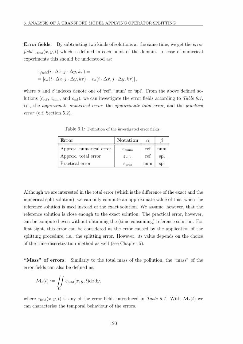
6. ANALYSIS OF A TRANSPORT MODEL APPLYING OPERATOR SPLITTING
Error fields. By subtracting two kinds of solutions at the same time, we get the error
field εfield(x, y, t) which is defined in each point of the domain. In case of numerical
experiments this should be understood as:
εfield(i · ∆x, j · ∆y, kτ) =
= |cα(i · ∆x, j · ∆y, kτ) − cβ(i · ∆x, j · ∆y, kτ)| ,
where α and β indeces denote one of ‘ref’, ‘num’ or ‘spl’. From the above defined so-
lutions (cref , cnum, and cspl), we can investigate the error fields according to Table 6.1,
i.e., the approximate numerical error, the approximate total error, and the practical
error (c.f. Section 5.2).
Table 6.1: Definition of the investigated error fields.
Error Notation α β
Approx. numerical error εanum ref num
Approx. total error εatot ref spl
Practical error εprac num spl
Although we are interested in the total error (which is the difference of the exact and the
numerical split solution), we can only compute an approximate value of this, when the
reference solution is used instead of the exact solution. We assume, however, that the
reference solution is close enough to the exact solution. The practical error, however,
can be computed even without obtaining the (time consuming) reference solution. For
first sight, this error can be considered as the error caused by the application of the
splitting procedure, i.e., the splitting error. However, its value depends on the choice
of the time-discretization method as well (see Chapter 5).
“Mass” of errors. Similarly to the total mass of the pollution, the “mass” of the
error fields can also be defined as:
Mε(t) :=
∫∫
Ω
εfield(x, y, t)dxdy,
where εfield(x, y, t) is any of the error fields introduced in Table 6.1. With Mε(t) we
can characterise the temporal behaviour of the errors.
120

6.4. RESULTS ON THE ERROR FIELDS
Relative errors. The previously introduced mass errors Mε(t) can be divided by
the mass of the reference solution Mref(t). Then we can compute the corresponding
relative errors Rε(t) by the following way:
Rε(t) =Mε(t)
Mref(t).
For investigating the temporal behaviour of the different errors, this quantity is more
relevant than Mε(t), because in some way it is independent from the behaviour of the
solution. We interpret it by an example. Temporal growth of Mε(t) can happen either
because the error or the solution is increasing. Therefore, from the growth of Mε(t),
we cannot conclude that the error is increasing in time. However, temporal growth of
Rε(t) can only happen when the error is increasing faster than the solution.
6.4 Results on the error fields
In this section we present our results on the solutions and the different error fields ob-
tained by solving problem (6.1). In the case of the error fields, we plot the square-root
of the corresponding values for better visualisation.
Figure 6.3: Numerical solution of (6.1) with constant wind velocity (left
panel) and Molenkampf – Crowley advection (right panel). (Similar results are
obtained when applying splitting procedures.)
In Figure 6.3 the numerical solutions cnum of equation (6.1) can be seen using constant
wind velocity and the Molenkampf –Crowley advection, respectively. We note that we
121

6. ANALYSIS OF A TRANSPORT MODEL APPLYING OPERATOR SPLITTING
Figure 6.4: Approximate numerical error field in the case of Molenkampf –
Crowley advection.
Figure 6.5: Approximate total error field, for sequential splitting and
Molenkampf – Crowley advection, using the upwind scheme (left panel) and
the semi-Lagrangian scheme (right panel).
obtained similar results applying splitting procedures, as well.
In Figures 6.4 and 6.6 the approximate numerical error εanum, the approximate to-
tal error εatot, and the practical error εprac can be seen for sequential splitting and
Molenkampf –Crowley advection. Error fields εatot and εprac are shown in the cases
of upwind and semi-Lagrangian schemes, as well. We note that applying the Strang
splitting, we obtained error fields having similar structure, but the values are less than
in the case of sequential splitting. The reason is that the sequential splitting is of first
122
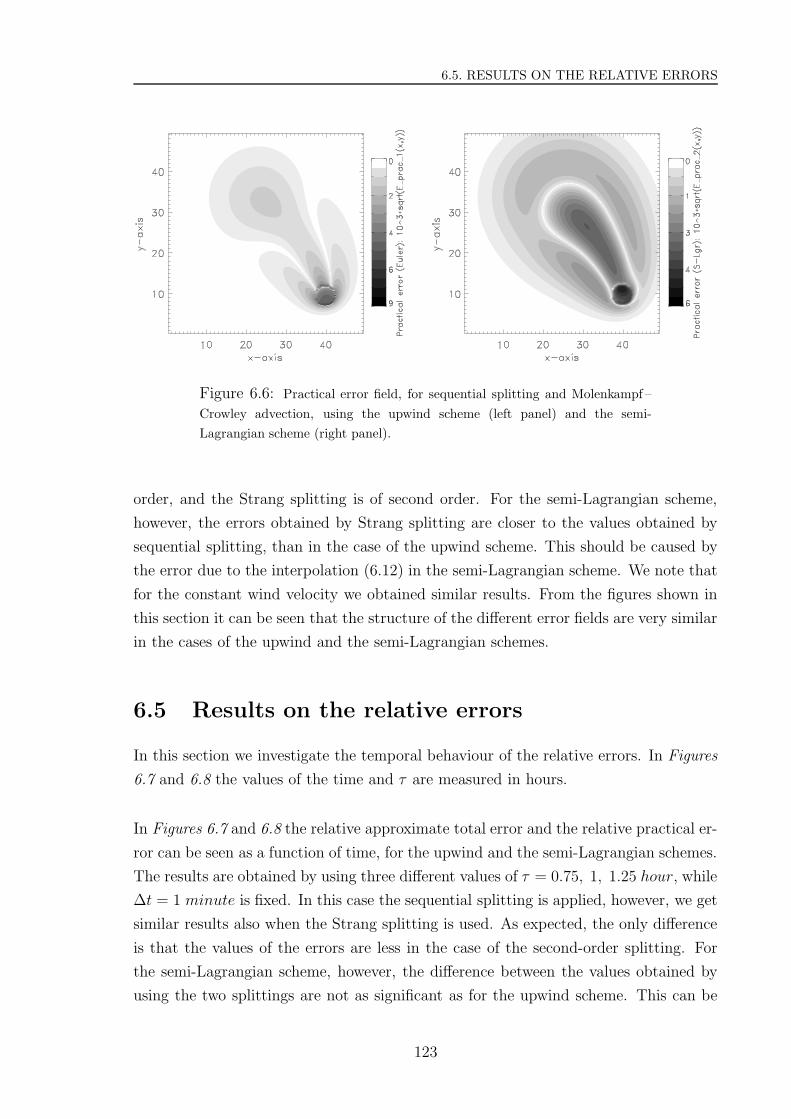
6.5. RESULTS ON THE RELATIVE ERRORS
Figure 6.6: Practical error field, for sequential splitting and Molenkampf –
Crowley advection, using the upwind scheme (left panel) and the semi-
Lagrangian scheme (right panel).
order, and the Strang splitting is of second order. For the semi-Lagrangian scheme,
however, the errors obtained by Strang splitting are closer to the values obtained by
sequential splitting, than in the case of the upwind scheme. This should be caused by
the error due to the interpolation (6.12) in the semi-Lagrangian scheme. We note that
for the constant wind velocity we obtained similar results. From the figures shown in
this section it can be seen that the structure of the different error fields are very similar
in the cases of the upwind and the semi-Lagrangian schemes.
6.5 Results on the relative errors
In this section we investigate the temporal behaviour of the relative errors. In Figures
6.7 and 6.8 the values of the time and τ are measured in hours.
In Figures 6.7 and 6.8 the relative approximate total error and the relative practical er-
ror can be seen as a function of time, for the upwind and the semi-Lagrangian schemes.
The results are obtained by using three different values of τ = 0.75, 1, 1.25 hour, while
∆t = 1 minute is fixed. In this case the sequential splitting is applied, however, we get
similar results also when the Strang splitting is used. As expected, the only difference
is that the values of the errors are less in the case of the second-order splitting. For
the semi-Lagrangian scheme, however, the difference between the values obtained by
using the two splittings are not as significant as for the upwind scheme. This can be
123
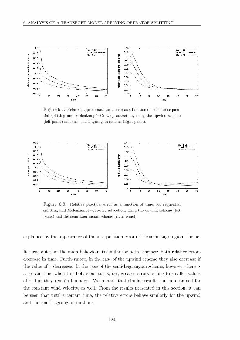
6. ANALYSIS OF A TRANSPORT MODEL APPLYING OPERATOR SPLITTING
Figure 6.7: Relative approximate total error as a function of time, for sequen-
tial splitting and Molenkampf –Crowley advection, using the upwind scheme
(left panel) and the semi-Lagrangian scheme (right panel).
Figure 6.8: Relative practical error as a function of time, for sequential
splitting and Molenkampf – Crowley advection, using the upwind scheme (left
panel) and the semi-Lagrangian scheme (right panel).
explained by the appearance of the interpolation error of the semi-Lagrangian scheme.
It turns out that the main behaviour is similar for both schemes: both relative errors
decrease in time. Furthermore, in the case of the upwind scheme they also decrease if
the value of τ decreases. In the case of the semi-Lagrangian scheme, however, there is
a certain time when this behaviour turns, i.e., greater errors belong to smaller values
of τ , but they remain bounded. We remark that similar results can be obtained for
the constant wind velocity, as well. From the results presented in this section, it can
be seen that until a certain time, the relative errors behave similarly for the upwind
and the semi-Lagrangian methods.
124

6.6. COMPARISON OF CPU TIMES
6.6 Comparison of CPU times
As we have already mentioned, the advantage of the semi-Lagrangian scheme for solving
the advection sub-model is that it needs less computational work than the upwind
scheme, because it uses large time step (which equals the splitting time step). This
means that using it, the integration of the model’s equation should take less CPU time.
0
50
100
150
200
250
300
350
400
0 10 20 30 40 50 60 70
CP
U ti
me
(sec
)
time
without splittingsplitting with upwindsplitting with semi-Lagrangian
0
50
100
150
200
250
300
350
400
0 10 20 30 40 50 60 70
CP
U ti
me
(sec
)
time
without splittingsplitting with upwindsplitting with semi-Lagrangian
Figure 6.9: CPU times (in seconds) in the cases when no splitting is applied,
and when the sequential splitting (left panel) or the Strang splitting (right
panel) is applied together the upwind and the semi-Lagrangian scheme, respec-
tively. (Constant wind velocity is used, but we get similar behaviour also in
the case of the Molenkampf –Crowley advection.)
In Figure 6.9 the CPU times can be seen as a function of time t ∈ [0, T ] in the cases
when no splitting is applied, and when the sequential and the Strang splittings are ap-
plied, respectively, together with the upwind and the semi-Lagrangian schemes. One
can see that using the upwind scheme, the integration takes more time than when no
splitting is applied. However, by using the semi-Lagrangian scheme with large time
step, the integration needs less CPU time.
One can see that the integration without splitting and applying splitting together with
the upwind scheme takes more CPU time in the case of the Strang splitting than in the
case of the sequential splitting. This is expected from the formulae (2.5) and (2.10) of
the splittings, because more sub-problems have to be solved in the case of the Strang
splitting. However, by comparing the figures, this behaviour cannot be observed when
the semi-Lagrangian scheme is used, i.e., the difference between the CPU times for the
two splittings is very small. This means that it is worth using the semi-Lagrangian
125
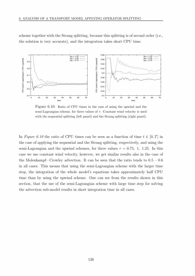
6. ANALYSIS OF A TRANSPORT MODEL APPLYING OPERATOR SPLITTING
scheme together with the Strang splitting, because this splitting is of second order (i.e.,
the solution is very accurate), and the integration takes short CPU time.
0.4
0.5
0.6
0.7
0.8
0.9
1
0 10 20 30 40 50 60 70
CP
U (
sem
i-Lag
ram
gian
) / C
PU
(up
win
d)
time
tau = 1.25tau = 1.00tau = 0.75
0.5
0.52
0.54
0.56
0.58
0.6
0.62
0.64
0.66
0.68
0 10 20 30 40 50 60 70C
PU
(se
mi-L
agra
mgi
an)
/ CP
U (
upw
ind)
time
tau = 1.25tau = 1.00tau = 0.75
Figure 6.10: Ratio of CPU times in the case of using the upwind and the
semi-Lagrangian scheme, for three values of τ . Constant wind velocity is used
with the sequential splitting (left panel) and the Strang splitting (right panel).
In Figure 6.10 the ratio of CPU times can be seen as a function of time t ∈ [0, T ] in
the case of applying the sequential and the Strang splitting, respectively, and using the
semi-Lagrangian and the upwind schemes, for three values τ = 0.75, 1, 1.25. In this
case we use constant wind velocity, however, we get similar results also in the case of
the Molenkampf –Crowley advection. It can be seen that the ratio tends to 0.5 – 0.6
in all cases. This means that using the semi-Lagrangian scheme with the larger time
step, the integration of the whole model’s equations takes approximately half CPU
time than by using the upwind scheme. One can see from the results shown in this
section, that the use of the semi-Lagrangian scheme with large time step for solving
the advection sub-model results in short integration time in all cases.
126

Conclusions
In the thesis we have dealt with the theoretical and numerical study of splitting pro-
cedures. Application of these procedures means that the spatial differential operator
appearing in a partial differential equation is split into more sub-operators having
simpler structure (corresponding e.g. to different physical phenomena). The numerical
solution of the problem is then obtained by combining the solutions of the sub-problems
corresponding to the sub-operators. We have investigated the sequential, Strang, and
weighted splittings in more details.
Since operator splitting procedures are time-discretization methods, the question of
their convergence is crucial, thus, we have studied under which conditions the numer-
ical solution of the split problem tends to the exact solution of the original problem
when the splitting time step decreases. Convergence of the splitting procedures is
studied in the framework of the operator semigroup theory. We have assumed the
sub-operators and their sum to be the generators of strongly continuous semigroups on
the corresponding domains and on the closure of their intersection, respectively. For
this case there exist results in the literature. The Trotter Product Formula means the
convergence of the sequential splitting, while Chernoff’s Theorem states a more general
case, and with its help the convergence of the Strang and weighted splittings can be
proven. We have shown that the stability condition is the same for the three splittings,
and it implies their convegence.
We have studied the convergence also in the case when spatial discretization methods
are used to solve the sub-problems, and the semigroups are approximated by sequences
of semigroups tending to them. The case when the semigroups are approximated by
operators describing not only spatial but also time-discretization methods, can be sim-
ilarly treated. As expected from the numerical analysis, these methods have to be
stable, consistent, and convergent.
127
CONCLUSIONS
We have used the above results in order to show the covergence of the splittings ap-
plied to abstract delay equations. The convergence has been illustrated by numerical
experiments as well. As another application of splitting procedures, I have presented
an idea how to shorten the computational time of an air pollution transport model. I
have developed a computer code to show that if different time steps are used for the
different sub-problems, less computational steps are needed.
128

Bibliography
[1] K. Atkinson, W. Han, Theoretical Numerical Analysis: A Functional Analysis
Framework, Springer, New York. (2005)
[2] K. A. Bagrinovskii, S. K. Godunov, Difference schemes for multidimensional prob-
lems (in Russian), Dokl. Akad. Nauk. USSR 115, 431–433. (1957)
[3] A. Batkai, S. Piazzera, Semigroups for Delay Equations, A K Peters, Wellesley,
Massachusetts. (2005)
[4] A. Batkai, P. Csomos, and G. Nickel, Splitting and approximations for delay
equations (in preparation).
[5] M. Bjørhus, Operator splitting for abstract Cauchy problems, IMA J. Numerical
Analysis 18, 419–443. (1998)
[6] P. R. Chernoff, Note on product formulas for operator semigroups, J. Functional
Analysis 2, 238–242. (1968)
[7] P. R. Chernoff, Product Formulas, Nonlinear Semigroups and Addition of Un-
bounded Operators, Memoirs of American Mathematical Society 140. (1974)
[8] C. I. Christov and R. S. Marinova, Implicit vectorial operator splitting for in-
compressible Navier – Stokes equations in primitive variables, J. Computational
Technologies 6 (4), 92–119. (2001)
[9] P. Csomos: Analytical solutions and numerical experiments for optimizing oper-
ator splitting procedures, Idojaras, Quarterly J. of the Hungarian Meteorological
Service 110 3-4., 379–415. (2006)
[10] P. Csomos, Operator splitting procedures for air pollution transport models, Lec-
ture Notes in Computational Sciences 3743, Springer–Verlag, 331–338. (2006)
129

BIBLIOGRAPHY
[11] P. Csomos, Some aspects of interaction between splitting procedures and numerical
methods, in K. Georgiev et al. (Eds.), NATO ARW Advances in Air Pollution
Modelling for Environmental Security, NATO Science Series, Springer-Verlag, 77–
91. (2005)
[12] P. Csomos, Analysis of a transport model applying operator splitting and semi-
Lagrangian method, Int. J. Computational Science and Engineering (to appear).
[13] P. Csomos, I. Farago, and A. Havasi, Weighted sequential splittings and their
analysis, Computers and Mathematics with Applications 50, 1017–1031. (2005)
[14] P. Csomos, I. Dimov, I. Farago, A. Havasi, and Tz. Ostromsky, Computational
complexity of weighted splitting scheme on parallel computers, Int. J. Parallel,
Emergent and Distributed Systems 223, 137–147. (2007)
[15] P. Csomos, I. Farago, Error analysis of the numerical solution of split differential
equations, Mathematical and Computer Modelling (to appear).
[16] P. Csomos, G. Nickel, Operator splittings for delay equations, Computers and
Mathematics with Applications (to appear).
[17] P. Csomos, I. Farago, A. Havasi, Operator splitting and global error analysis, in
D. Melas and D. Syrakov (Eds.), NATO ARW Air Pollution Processes in Regional
Scale, Kluwer Academic Publishers, 37–44. (2002)
[18] P. Csomos, E. Sikolya, Numerical methods for split differential equations (in prepa-
ration).
[19] R. Courant, K. Friedrichs, and H. Lewy, Uber die partiellen Differenzengleichungen
der mathematischen Physik, Mathematische Annalen 100, 32–74. (1928)
[20] I. Dimov, Z. Zlatev Computational and Numerical Challenges in Environmental
Modelling, Elsevier, Amsterdam. (2006)
[21] I. Dimov, I. Farago, A. Havasi, and Z. Zlatev, Different splitting techniques with
application to air pollution transport models, Int. J. Environmental Pollution (to
appear).
[22] K. – J. Engel, R. Nagel, One-Parameter Semigroups for Linear Evolution Equa-
tions, Springer–Verlag, Berlin. (2000)
130

BIBLIOGRAPHY
[23] K. – J. Engel, R. Nagel, A Short Course on Operator Semigroups Springer–Verlag,
New York. (2005)
[24] I. Farago, Splitting methods and their application to the abstract Cauchy prob-
lems, Lecture Notes in Computational Sciences 3401, Springer–Verlag 35–45.
(2005)
[25] I. Farago, New operator splitting methods and their applications, in: Boyanov et
al. (Eds.) “Numerical Methods and Applications”, Lecture Notes in Computational
Sciences 4310, Springer–Verlag, Berlin, 443–450 (2007).
[26] I. Farago, A modified iterated operator splitting method, Applied Mathematical
Modelling (to appear).
[27] I. Farago, J. Geiser, Iterative operator splitting methods for linear problems,
Weierstrass Intitut fur Angewandte Analysis 1043, 1–18., Int. J. Computational
Science and Engineering (to appear).
[28] I. Farago, A. Havasi, On the convergence and local splitting error of different
splitting schemes, Progress in Computational Fluid Dynamics 5, 495–504. (2005)
[29] I. Farago, A. Havasi, Consistency analysis of operator splitting methods for C0-
semigroups, Semigroup Forum 74, 125–139. (2007)
[30] I. Farago, M. Kovacs, On maximum norm contractivity of second order damped
single step methods, Calcolo 40, 91–108. (2003)
[31] S. Flory, F. Neubrander, and Y. Zhuang, On the regularization and stabilization
of approximation schemes for C0-semigroups, Operator Theory Adv. Appl. 126,
119–132. (2001)
[32] S. Flory, F. Neubrander, and L. Weis, Consistency and stabilization of ratio-
nal approximation schemes for C0-semigroups, Progress in Nonlinear Differential
Equations 55, 181–193. (2003)
[33] A. Hansbo, Nonsmooth error estimates for damped single step methods for
parabolic equations in Banach space, Calcolo 36, 75–101. (1999)
[34] A. Havasi, J. Bartholy, and I. Farago, Splitting method and its aplication in
air pollution modelling, Idojaras, Quarterly J. of the Hungarian Meteorological
Service 105, 39–58. (2001)
131
BIBLIOGRAPHY
[35] Z. Horvath, On the positivity step size threshold of Runge –Kutta methods, Ap-
plied Numerical Mathematics 53, 341–356. (2005)
[36] W. Hundsdorfer, J. G. Verwer, Numerical Solution of Time-dependent Advection–
Diffusion–Reaction Equations, Springer–Verlag, Berlin. (2003)
[37] T. Ichinose, H. Tamura, H. Tamura, and V. A. Zagrebnov, Note on the Paper
“The norm convergence of the Trotter – Lie product formula with error bound”
by Ihinose and Tamura, Communications in Mathematical Physics 221, 499–510.
(2001)
[38] K. Ito, F. Kappel, Evolution Equations and Approximations, World Scientific,
River Edge, N. J. (2002)
[39] K. Ito, F. Kappel, The Trotter –Kato theorem and approximation of PDE’s, Math-
ematics of Computation 67 No. 221, 21–44. (1998)
[40] E. R. Jakobsen, K. Hvistendahl Karlsen and N. H. Risebro, On the convergence
rate of operator splitting for Hamilton – Jacobi equations with source terms, SIAM
J. Numerical Analysis 39 (2), 499–518. (2001)
[41] T. Jahnke, Ch. Lubich, Error bounds for exponential operator splittings, BIT 40,
735–744. (2000)
[42] F. Kappel, Semigroups and delay equations, in: H. Brezis et al. (Eds.) “Semi-
groups, Theory and Application” Vol. II., Pitman Research Notes in Mathematics
152, Longman, 136–176. (1986)
[43] K. Hvistendahl Karlsen, N. H. Risebro, Unconditionally stable methods for Hamil-
ton – Jacobi equations, J. Computational Physics 180 (2), 710–735. (2002)
[44] K. Hvistendahl Karlsen, K. –A. Lie, J. R. Natvig, H. F. Nordhaug, and
H. K. Dahle, Operator splitting methods for systems of convection–diffusion equa-
tions: nonlinear error mechanisms and correction strategies, J. Computational
Physics 173, 636–663. (2001)
[45] T. Kato, On the Trotter – Lie product formula, Proceedings of the Japan Academy
50, 694–698. (1974)
[46] J. D. Lambert, Numerical Methods for Ordinary Differential Systems, John Wiley
& Sons, Chicester. (1991)
132
BIBLIOGRAPHY
[47] L. D. Landau, E. M. Lifshitz, Course on Theoretical Physics, 1: Mechanics, Perg-
amon Press, Oxford. (1958)
[48] P. D. Lax, Functional Analysis, John Wiley & Sons, New York. (2002)
[49] G. I. Marchuk, Some application of splitting-up methods to the solution of math-
ematical physics problems, Applik. Mat. 13 (2), 103–132. (1968)
[50] G. I. Marchuk, Methods of Numerical Mathematics, Springer–Verlag, Berlin.
(1982)
[51] R. S. Marinova, C. I. Christov, and T. T. Marinov, A fully coupled solver for
incompressible Navier – Stokes equations using operator splitting, Int. J. on Com-
putational Fluid Dynamics 17 (5), 371–385. (2003)
[52] M. Mimura, T. Nakaki and K. Tomoeda, A numerical approach to interface curves
for some nonlinear diffusion equations, Japanese J. Applied Mathematics 1, 93-
139. (1984)
[53] H. Neidhardt, V. A. Zagrebnov, On error estimates for the Trotter –Kato product
formula, Letters in Mathematical Physics 44, 169–186. (1998)
[54] H. Neidhardt, V. A. Zagrebnov, Trotter –Kato product formula and operator-norm
convergence, Communications in Mathematical Physics 205, 129–159. (1999)
[55] A. Pazy, Semigroups of Linear Operators and Applications to Partial Differential
Equations, Springer–Verlag, New York. (1983)
[56] R. Richtmyer, K. W. Morton, Difference Methods for Initial Value Problems.
Krieger Publishing, Malabar. (1994)
[57] B. Sportisse, An analysis of operator splitting techniques in the stiff case, J. Com-
putational Physics 161, 140–168. (2000)
[58] G. Stoyan, G. Tako, Numerical Methods (in Hungarian), ELTE–Typotex, Bu-
dapest. (1997)
[59] G. Strang, On the construction and comparison of difference schemes, SIAM J. Nu-
merical Anaysis., September, Vol. 5, No. 3, 506–517. (1968)
[60] G. Strang, Approximation of semigroups and the consistency of different schemes,
Proceedings of the American Mathematical Society 20, 1–7. (1969)
133

BIBLIOGRAPHY
[61] H. F. Trotter, Approximation of semi-groups of operators, Pacific J. Mathematics
8, 887–919. (1958)
[62] H. F. Trotter, On the product of semigroups of operators, Proceedings of the
American Mathematical Society 10, 545–551 (1959)
[63] V. S. Varadarajan, Lie Groups, Lie Algebras, and Their Representation, Springer–
Verlag, New York. (1984)
[64] G. F. Webb, Functional differential equations and nonlinear semigroups in Lp-
spaces, J. Differential Equations, 20, 71–89. (1976)
[65] A. Wiin –Nielson, On the application of trajectory methods in numerical forecast-
ing, Tellus, 11, 180–196. (1959)
[66] V. A. Zagrebnov, Topics in the Theory of Gibbs Semigroups, Leuven University
Press. (2003)
[67] Z. Zlatev, Computer Treatment of Large Scale Air Pollution Models, Kluwer Aca-
demic Publishers, Dordrecht. (1995)
[68] Z. Zlatev, J. Brandt, Testing variational data assimilation modules, in: I. Lirkov et
al. (Eds.) “Large-Scale Scientific Computing”, Springer–Verlag, Berlin, 395–402.
(2006)
134

Koszonetnyilvanıtas
Koszonom temavezetomnek, Farago Istvannak, hogy meglatta bennem azt, amit en
remelni sem mertem. Orok halaval tartozom Rainer Nagelnak, amiert engem is be-
fogadott tanıtvanyainak nepes korebe, es nem csak szellememet, de lelkemet is gaz-
dagıtotta. Koszonom Sikolya Eszternek, Batkai Andrasnak es Gregor Nickelnek, hogy
joval tobbek voltak szamomra, mint munkatarsak. Koszonettel tartozom a Tubingeni
Egyetem Funkcionalanalızis Tanszekenek, hogy egy eletreszolo elmennye varazsoltak
szamomra az ott eltoltott idot. Kulon koszonet illeti Horanyi Andrast a doktori
tanulmanyaim befejezesekor tanusıtott turelmeert, es a dolgozat beadasaban nyujtott
segıtsegeert. Es nem utolso sorban koszonom Sandor Zsoltnak, hogy mindvegig tama-
szom maradt a ,,hosszu harc alatt”.
Danksagung
Ich bedanke mich bei meinem Betreuer, Istvan Farago dafur, dass er mehr in mir gese-
hen hat, als ich jemals zu hoffen gewagt habe. Rainer Nagel hat mich zu unermasslichem
Dank verpflichtet, weil er mich in die große Familie seiner Studenten aufgenommen hat,
und er hat nicht nur meinen Geist, sondern auch meine Seele bereichert. Ich danke
Eszter Sikolya, Andras Batkai und Gregor Nickel dafur, mehr als nur meine Kollegen
zu sein. Ich schulde den Mitgliedern der Arbeitsgemeinschaft Funktionalanalysis der
Universitat Tubingen Dank, weil sie meinen Aufenthalt dort ein unvergessliches Erleb-
nis gezaubert haben. Besonderen Dank verdient Andras Horanyi fur seine Geduld und
Hilfe bei der Einreichung meiner Doktorarbeit. Und nicht zuletzt gilt mein Dank Zsolt
Sandor, der fur mich wahrend der ganzen Zeit eine feste Unterstutzung gewesen ist.
135

Osszefoglalas
Doktori ertekezesemben az operatorszeletelesi eljarasok elmeleti es numerikus vizsga-
lataval foglakozom. Ezen eljarasok alkalmazasakor a vizsgalt parcialis differencial-
egyenlet terbeli derivaltakat tartalmazo operatorat valamilyen szempont szerint (pl. a
fizikai folyamatoknak megfelelo) reszoperatorokra bontjuk fel. Az egyenlet numerikus
megoldasat az egyes reszoperatorok altal meghatarozott problemak megoldasaibol szar-
maztatjuk. A szarmaztatas modja szerint megkulonboztetjuk a szekvencialis, a Strang
es a sulyozott operatorszeletelesi eljarasokat.
Mint minden numerikus modszer eseten, az operatorszeletelesi eljarasoknal is elsodleges
fontossagu a konvergencia, azaz azon kerdes viszgalata, tart-e a numerikus megoldas
a problema pontos megoldasahoz a modszer lepeskozenek csokkentesekor. Az ope-
ratorszeletelesi eljarasok konvergenciajat az operatorfelcsoport-elmelet keretei kozott
tanulmanyozom. Feltetelezem, hogy az absztakt Cauchy-problema jobb oldalan szerep-
lo ket generator osszege is general egy erosen folytonos felcsoportot az ertelmezesi tar-
tomanyok metszetenek lezartjan. Erre az esetre mar leteznek eredmenyek az irodalom-
ban: a Trotter-fele szorzat-formula eppen a szekvencialis szeleteles konvergenciajat
jelenti, mıg a Chernoff-tetel egy altalanosabb esetrol szol, es segıtsegevel a Strang-fele
es a sulyozott szeleteles konvergenciaja is bizonyıthato. Megmutatom, hogy a konver-
gencia feltetele a stabilitasi kriterium teljesulese, mely mindharom vizsgalt szeleteles
eseten kovetkezik a szekvencialis szeleteles stabilitasi kriteriumabol.
A konvergenciat vizsgalom abban az esetben is, amikor a reszoperatorokra terbeli app-
roximacios semat alkalmazok. Ekkor a reszoperatorok altal generalt felcsoportokat
hozzajuk konvergalo felcsoportokkal kozelıtem. Hasonlokeppen bizonyıthato az az
eset is, amikor a felcsoportokat az idobeli es terbeli numerikus semaknak megfelelo
operatorokkal kozelıtem. Mint az a numerikus analızis elmeletebol varhato, ekkor a
numerikus modszereknek stabilnak, konzisztensnek es konvergensnek kell lenniuk.
Mindezen eredmenyeket alkalmazom kesleltetest tartalmazo differencialegyenletekre.
A konvergencia bizonyıtasa utan eredmenyeimet az altalam kifejlesztett szamıtogepes
program segıtsegevel szemleltetem. Tovabbi alkalmazaskent a szinten altalam fejlesztett,
a legszennyezes terjedeset leıro modellt mutatom be. Megvizsgalom annak a lehetoseget,
hogy az operatorszeleteles alkalmazasaval hogyan lehet csokkenteni a modell szamıtasi
(azaz futasi) idejet.
137

Summary
In my PhD thesis I have dealt with the theoretical and numerical study of splitting
procedures. Application of these procedures means that the spatial differential opera-
tor appearing in a partial differential equation is split into more sub-operators having
simpler structure (corresponding e.g. to physical phenomena). The numerical solution
of the problem is then obtained by combining the solutions of the sub-problems corre-
sponding to the sub-operators. I have investigated the sequential, Strang, and weighted
splittings.
Since operator splitting procedures are time-discretization methods, the question of
their convergence is crucial, thus, I have studied under which conditions the numerical
solution of the split problem tends to the exact solution of the original problem when
the splitting time step decreases. Convergence of the splitting procedures is studied
in the framework of the operator semigroup theory. I have assumed the sub-operators
and their sum to be the generators of strongly continuous semigroups on the corre-
sponding domains and on the closure of their intersection, respectively. For this case
there exist already results in the literature. The Trotter Product Formula means the
convergence of the sequential splitting, while Chernoff’s Theorem states a more general
case, and with its help the convergence of the Strang and weighted splittings can be
proven. I have shown that the stability conditions of the Strang and weighted splitting
procedures follow from the stability criterion of the sequential splitting, and it implies
their convegence.
I have studied the convergence also in the case when spatial discretization methods are
used to solve the sub-problems, and the semigroups are approximated by sequences of
semigroups tending to them. The case can be similarly treated when the semigroups
are approximated by operators describing not only spatial but also time-discretization
methods. As expected from the theory of numerical analysis, these methods have to
be stable, consistent, and convergent.
I have used the above results in order to show the covergence of the splittings applied
to abstract delay equations. The convergence has been illustrated by numerical ex-
periments as well. As another application of splitting procedures, I have presented an
idea how to shorten the computational time of an air pollution transport model. I
have developed a computer code to show that if different time steps are used for the
different sub-problems, less computational steps are needed.
139