Theoretical and Experimental Studies of Seafloor Backscatter
49
Author: Maria Desamparados Torres Medina 1, 2 Directors: Iain Michael Parnum 3, 4 , Alexander Gavrilov 3, 5 Co-director: Víctor Espinosa Roselló 1, 6 1 Universitat Politècnica de València, Escola Politecnica Superior de Gandia, València, Spain, [email protected] 2 , [email protected] 6 Centre for Marine Science and Technology, Curtin University of Technology, Perth, Western Australia, Australia, [email protected] 4 , [email protected] 5 Abstract Analysis of seafloor backscatter collected from single and multi beam echosounders (SBES and MBES) has been carried out using a theoretical model and experimental data. The aim of this work was to evaluate backscatter parameters for the purposes of seafloor habitat classification. A theoretical model developed by CMST was used to study the backscatter properties depending on seafloor properties, depth and transmit pulse width. Peak intensity and energy calculated from the predicted mean envelop for different sediment types were shown to be proportional to the backscatter coefficient. Integration of the tail of the envelope, which results in a commonly used backscatter parameter E1, shows that accurate calculation of the insonfication area is required to make it independent of depth. The effective pulse width of seafloor echoes was found to be proportional to the backscatter coefficient and highly dependent on the transmit pulse width and depth. Experimental measurements using a Simrad EQ60 single beam echo-sounder, operating at 38 and 200 kHz, were made to distinguish different seafloor habitats. The energy and parameter E1 at 200 kHz were the most useful parameters for discriminating different seafloor habitats and the resulting classification was consistent between different transects across the same area of the seafloor. In addition, temporal variations of backscatter from seagrass were studied. This experiment showed unexpectedly small temporal variations in the mean backscatter characteristics, both intensity and energy, at 200 kHz. Subtle diurnal variations were observed in the mean backscatter intensity at 38 kHz. Statistics of backscatter from seagrass was analysed at both frequencies pointing out a complex, rather bimodal distribution observed in the fluctuations of the instantaneous backscatter intensity. Author: Maria Desamparados Torres Medina, email: [email protected] Date of issue: July 2010 Theoretical and Experimental Studies of Seafloor Backscatter
Transcript of Theoretical and Experimental Studies of Seafloor Backscatter
Author: Maria Desamparados Torres Medina1, 2
Directors: Iain Michael Parnum3, 4
, Alexander Gavrilov3, 5
Co-director: Víctor Espinosa Roselló1, 6
1Universitat Politècnica de València, Escola Politecnica Superior de Gandia, València, Spain, [email protected],
Centre for Marine Science and Technology, Curtin University of Technology, Perth, Western Australia, Australia,
[email protected] , [email protected]
Abstract
Analysis of seafloor backscatter collected from single and multi beam echosounders (SBES and MBES) has been
carried out using a theoretical model and experimental data. The aim of this work was to evaluate backscatter
parameters for the purposes of seafloor habitat classification. A theoretical model developed by CMST was used
to study the backscatter properties depending on seafloor properties, depth and transmit pulse width. Peak
intensity and energy calculated from the predicted mean envelop for different sediment types were shown to be
proportional to the backscatter coefficient. Integration of the tail of the envelope, which results in a commonly
used backscatter parameter E1, shows that accurate calculation of the insonfication area is required to make it
independent of depth. The effective pulse width of seafloor echoes was found to be proportional to the
backscatter coefficient and highly dependent on the transmit pulse width and depth. Experimental measurements
using a Simrad EQ60 single beam echo-sounder, operating at 38 and 200 kHz, were made to distinguish different
seafloor habitats. The energy and parameter E1 at 200 kHz were the most useful parameters for discriminating
different seafloor habitats and the resulting classification was consistent between different transects across the
same area of the seafloor. In addition, temporal variations of backscatter from seagrass were studied. This
experiment showed unexpectedly small temporal variations in the mean backscatter characteristics, both intensity
and energy, at 200 kHz. Subtle diurnal variations were observed in the mean backscatter intensity at 38 kHz.
Statistics of backscatter from seagrass was analysed at both frequencies pointing out a complex, rather bimodal
distribution observed in the fluctuations of the instantaneous backscatter intensity.
Author: Maria Desamparados Torres Medina, email: [email protected]
Date of issue: July 2010
Theoretical and Experimental Studies of
Seafloor Backscatter

2 Theoretical and Experimental Studies of Seafloor Backscatter
INDEX
I. INTRODUCTION ............................................................................................................................ 4
1. Motivation ................................................................................................................................ 4
2. Aims and scope of the study ..................................................................................................... 5
II. BACKGROUND THEORY ............................................................................................................. 7
1. Physics of sound and scattering ............................................................................................... 7
Introduction ......................................................................................................................... 7
Reflection and scattering ..................................................................................................... 7
Bubbles ................................................................................................................................ 7
2. Single beam systems ............................................................................................................... 10
Operation ........................................................................................................................... 11
Acoustic Seafloor Classification ........................................................................................ 12
III. MODELING SINGLE BEAM ECHO SOUNDER BACKSCATTER ......................................... 14
1. Introduction ............................................................................................................................ 14
2. Model description ................................................................................................................... 14
3. Correlation of single beam backscatter characteristics with the seafloor backscatter
coefficient ..................................................................................................................................... 16
4. Dependence of single beam backscatter characteristics on sea depth .................................. 17
5. Dependence of single beam backscatter characteristics on pulse width ............................... 19
6. Discussion .............................................................................................................................. 20
IV. MEASURING BACKSCATTER FROM DIFFERENT HABITATS ........................................... 21
1. Introduction ............................................................................................................................ 21
2. Methods .................................................................................................................................. 21
Data collection ................................................................................................................... 21
Data processing ................................................................................................................. 22
Data analysis ..................................................................................................................... 23
3. Results .................................................................................................................................... 23
Owen Anchorage - SBES depth and backscatter parameters ............................................ 23
Morinda Shoal - SBES depth and backscatter parameters ................................................ 26
Analysis of the distribution function - Owen Anchorage ................................................... 28
4. Conclusions ............................................................................................................................ 29
V. TEMPORAL VARIABILITY OF BACKSCATTER FROM SEAGRASS .................................. 30
1. Introduction ............................................................................................................................ 30
2. Methods .................................................................................................................................. 30
3. Backscatter from seagrass and its long-term variations ........................................................ 31
4. Statistical analysis of short-term fluctuations ........................................................................ 34
5. Conclusions ............................................................................................................................ 38
VI. CONCLUSIONS ............................................................................................................................ 40
FUTURE WORK .................................................................................................................................. 41
ACKNOWLEDGMENT ........................................................................................................................ 41
BIBLIOGRAPHY .................................................................................................................................. 42
APPENDIX ............................................................................................................................................ 41

Theoretical and Experimental Studies of Seafloor Backscatter 3
A tot i tots el que han fet possible que esta experiencia fora real,
sobretot per als que estaven prop de mi.
Gràcies.
4 Theoretical and Experimental Studies of Seafloor Backscatter
I. INTRODUCTION
1. MOTIVATION
One of the key challenges in the study of the natural environment is determining what change is due to
natural variability and what can potentially be a result of anthropogenic impact to the system. Coastal
habitats, such as seagrass and coral reefs, are significant forces that shape our ecosystem and are
intrinsically linked with the overall health of the environment [1]. Coastline change has been
recognized as a likely future challenge to coastal management, due to the increased coastal utilization.
Measuring impacts from industrial contamination, urban growth and general nutrient enrichment on
coastal habitats, e.g. significant seagrass loss to the ecosystem, is not a trivial exercise. Therefore,
methods that can accurately measure change in the marine environment are required for effective
management of natural resources.
One such important coastal habitat is seagrass, as it: 1) plays a critical role in maintaining marine
biological productivity and biogeochemical cycles, e.g. through photosynthesis they produce large
quantities of oxygen [2]; 2) supports a high species diversity and commercial fisheries [3]; 3) creates
natural barriers, and thus strongly reduce coastal erosion; and 4) is an important indicator of
disturbance in the coastal marine environment. Hence, there is a scientific interest in and practical
importance of estimating the extent of existing stocks and measuring changes over time. However,
monitoring marine habitats, such as seagrass, is both economically and technically challenging.
Detection and measurements of submerged aquatic vegetation has been carried out using several
methods. These different methods can be grouped into two large types: direct sampling and remote
sensing techniques [5][7][8][9][10][11].
Many studies have a requirement for assessments of seabed type: defence related (e.g. mine
countermeasures), environmental (e.g. habitat mapping and protection), economic (e.g. fisheries,
mining), and maritime (e.g. dredging of harbours and channels). Remote sensing combined with direct
sampling methods (ground-truthing) is the most common approach to seafloor habitat mapping.
Acoustic remote sensing of the seafloor has been used to discriminate between different seafloor
habitats, particularly in deep or turbid waters where aerial remote sensing is not effective.
Acoustic remote sensing of the seafloor is usually carried out using a sonar (SOund, NAvigation and
Ranging) system, which is an instrument used for getting information about the underwater
environment through the transmission of sound waves and measuring the return echoes. Sonar mapping
systems are usually deployed from vessels and are operated while underway. Some of sonar systems

Theoretical and Experimental Studies of Seafloor Backscatter 5
can be used to determine the bottom type. Acoustic data usually require ground-truthing to help assign
seafloor types to any classification map produced. The results can also be dependent on echosounder
characteristics, such as frequency and beamwidth (discussed in the next chapter). One such sonar
mapping system is a Single Beam Echosounder (SBES). This type of echosounders is simple to use
and is found on most vessels. The primary purpose of the SBES is to measure the two-way travel time
of the signal, which gives the local water depth. In addition, the shape and amplitude of the echo
received can be used to derive information about the type of seabed. It is the use of the SBES in
seafloor classification that is the subject of this project. This study has analysed the energy and the
envelope of the received backscatter signal from SBES experimental data and model predictions, with
the purpose of improving the classification of seafloor habitats. Some data from a multibeam sonar
system have also been analysed.
2. AIMS AND SCOPE OF THE STUDY
There were two main aims of this study:
1. Evaluate different parameters derived from the backscatter envelope measured using a SBES to
determine the most useful backscatter characteristics for seafloor habitat classification.
2. Measure the temporal variability of backscatter characteristics of seagrass.
Following the introduction, this dissertation is divided into the following chapters:
Chapter 2: Background Theory. This presents a background to understanding the physics of
seabed backscatter, which is essential for the classification methods, as well as an explanation of
how SBES systems work and the signal backscattered from the seafloor is processed.
Chapter 3: Modelling seafloor backscatter envelopes from single beam echosounders. A
theoretical model was use to predict the shape of backscatter envelope received by SBES from
different kinds of sediment. The model was developed by the Centre for Marine Science and
Technology (CMST),at Curtin University of Technology in Perth, Australia. The CMST model uses
the Applied Physics Laboratory (APL) high-frequency bottom scattering model [34][35] to
determine the backscatter coefficient based on the sediment characteristics. Parameters derived
from the backscatter envelope, such as peak intensity and energy, were analysed with respect to
their dependence on the seafloor backscatter coefficient, sea depth and transmit pulse width to
determine their effectiveness in discriminating different seafloor types.

6 Theoretical and Experimental Studies of Seafloor Backscatter
Chapter 4: Analysis of single beam echosounder backscatter data collected from different
seafloor habitats. Data collected with a SBES over a sand-seagrass transition and over a coral reef-
sand-seagrass transition have been processed and analysed. The main focus of this chapter is the
correlation of backscatter parameters with changes in seafloor habitat type.
Chapter 5: Temporal variability of backscatter collected over seagrass. In the last part of the
dissertation, the objective was to determine whether there is time dependence in backscatter
collected over vegetated seafloors. Gas bubbles released from seagrass due to photosynthesis and/or
respiration are one of the most likely sources of strong acoustic scattering. If this is so, then the
backscatter level from seagrass could vary with time, as the rate of gas emission could change
during the day and in different seasons due to changes in the sun illumination. Using a Simrad
EQ60 single beam sonar, backscatter from bare sediment area (sand) and from dense seagrass
(Posidonea) was measured at 38 and 200 kHz every 2 s over 2 and 7 days respectively.
Chapter 6: Conclusions. The dissertation ends with a comparison of the study's findings with
results of other studies. Also, recommendations for further work in the field of acoustic seafloor
classification are made.
Theoretical and Experimental Studies of Seafloor Backscatter 7
II. BACKGROUND THEORY
1. PHYSICS OF SOUND AND SCATTERING
INTRODUCTION
Waves of sound energy oscillates back and forth in the direction the wave is travelling. They comprise
of alternative compressions and rarefactions that propagate at a speed that depends on the
characteristics of the medium, such as bulk density, compressional wave speed and attenuation [15].
Conceptually, a sound wave travelling diminishes in intensity over distance due to transmission loss
caused by spreading and absorption. The spherical spreading loss [42] is the major component which
causes this effect, implying that the intensity or the mean square pressure varies inversely with the
square of the distance from the source (e.g. sound levels diminishes 6dB when the distance is doubled).
In addition, when the sound wave interactions with the seafloor, “reflection” and “scattering” occur.
Reflection of a sound wave at a surface diffuses the wave out (with some energy loss) in a returned
wave with an equal angle to the angle of the incident wave (“specular direction”). Scattering produces
a distribution of acoustic energy over angles other that the incoming wave. The scattering returned to
the source (e.g. as in an echosounder) is referred to as backscatter. This chapter discusses what
influences backscatter, how it is measured using a single beam echosounder and how these backscatter
measurements can be used to identify seafloor habitats.
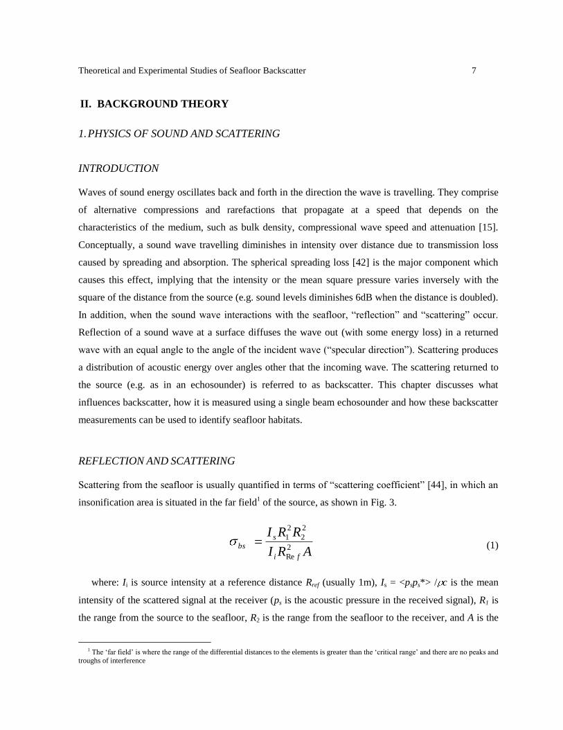
REFLECTION AND SCATTERING
Scattering from the seafloor is usually quantified in terms of “scattering coefficient” [44], in which an
insonification area is situated in the far field1 of the source, as shown in Fig. 3.
ARI
RRI
fi
sbs 2
Re
2
2
2
1 (1)
where: Ii is source intensity at a reference distance Rref (usually 1m), Is = <psps*> / c is the mean
intensity of the scattered signal at the receiver (ps is the acoustic pressure in the received signal), R1 is
the range from the source to the seafloor, R2 is the range from the seafloor to the receiver, and A is the
1 The „far field‟ is where the range of the differential distances to the elements is greater than the „critical range‟ and there are no peaks and
troughs of interference
8 Theoretical and Experimental Studies of Seafloor Backscatter
area of the scattering surface (<…> means statistical averaging). In this study, the scattering coefficient
is measured in a monostatic arrangement, and thus R1=R2. Loss of energy through absorption in the
water column must be taken into consideration at high frequencies. The absorption loss is usually
defined as R (dB), where is the absorption coefficient (dB/m). Consequently, for this study the
surface scattering coefficient is calculated as:
)log(20,)2exp(4
eAI
RRI
i
s
bs . (2)
The surface scattering coefficient is a dimensionless quantity that accounts for the intensity (power)
ratio of the incident and scattered waves determined per unit area at a reference distance of 1m. When
expressed in dB, it is commonly called the backscatter strength (BS):
)(log10 10 bsBS (3)
The level of backscatter strength measured from the seafloor is influenced by various properties,
such as the impedance contrast between the water column and seafloor, surface roughness and volume
heterogeneity (Fig. 1). For instance, high-porosity sediments, such as silts and clays have a low
acoustic impedance contrast with the overlying water so reflect and scatter considerably less energy
compared with high-density material like gravel and rock, which have a much higher impedance
contrast.
Fig. 1. Sketch showing acoustic scattering due to the roughness of the water sediment interface and
heterogeneity of the sediment. Image extracted from ref. 35.
Theoretical and Experimental Studies of Seafloor Backscatter 9
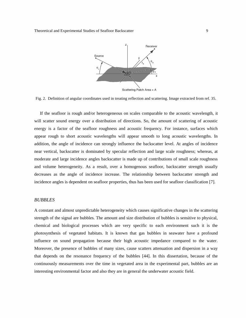
Fig. 2. Definition of angular coordinates used in treating reflection and scattering. Image extracted from ref. 35.
If the seafloor is rough and/or heterogeneous on scales comparable to the acoustic wavelength, it
will scatter sound energy over a distribution of directions. So, the amount of scattering of acoustic
energy is a factor of the seafloor roughness and acoustic frequency. For instance, surfaces which
appear rough to short acoustic wavelengths will appear smooth to long acoustic wavelengths. In
addition, the angle of incidence can strongly influence the backscatter level. At angles of incidence
near vertical, backscatter is dominated by specular reflection and large scale roughness; whereas, at
moderate and large incidence angles backscatter is made up of contributions of small scale roughness
and volume heterogeneity. As a result, over a homogenous seafloor, backscatter strength usually
decreases as the angle of incidence increase. The relationship between backscatter strength and
incidence angles is dependent on seafloor properties, thus has been used for seafloor classification [7].
BUBBLES
A constant and almost unpredictable heterogeneity which causes significative changes in the scattering
strength of the signal are bubbles. The amount and size distribution of bubbles is sensitive to physical,
chemical and biological processes which are very specific to each environment such it is the
photosynthesis of vegetated habitats. It is known that gas bubbles in seawater have a profound
influence on sound propagation because their high acoustic impedance compared to the water.
Moreover, the presence of bubbles of many sizes, cause scatters attenuation and dispersion in a way
that depends on the resonance frequency of the bubbles [44]. In this dissertation, because of the
continuously measurements over the time in vegetated area in the experimental part, bubbles are an
interesting environmental factor and also they are in general the underwater acoustic field.

10 Theoretical and Experimental Studies of Seafloor Backscatter
2. SINGLE BEAM ECHOSOUNDERS
A SOund NAvigation and Ranging (SONAR) system is an instrument used for getting information
about the underwater environment through the transmission and receiving of sound waves. One
common method to carry this out this is through electro-acoustic transducers, such as in single-beam
echosounders (SBES). In this dissertation, a SBES has been used to acquire backscatter information
from the seafloor. Although more sophisticated sonar systems (e.g. multi-beam sonar or sidescan sonar
systems) are available, they can be both cost and technically prohibited. Whereas, SBES are simple to
use and widespread on nearly all vessels.
A SBES system transmits vertically bellow the ship a short signal in a beam of average angular
aperture (Fig. 4). The system measures the two-way travel time of the signal, which gives the local
water depth and can provide information about the kind of seabed or detecting fish, depending on the
selected frequency. The first return from the seabed corresponds to points closest to the ship, and
further as the cone spreads contributions from sub-surface penetration and, if present, overlying biota
such as seagrass.
Dφ
πDcT
A = π (D tan (Φ))2 (4)
Fig. 3. Schematic representation of the insonification of the seafloor from a SBES.
Where: D equal to depth and Φ equals to half-power beam width. It is important to know the
characteristics of the produced insonified area. The area insonified on the seafloor by a SBES (A) is
dependent on the beam width, water depth and the local slope (Eq. .
Theoretical and Experimental Studies of Seafloor Backscatter 11
Because of wavefront curvature a ping from an echo-sounder with a wide angle beam ensonifies
first a circle on the seabed, then progressively ensonifies an annuli of increasing radii and higher
incidence angles (Fig. 3.).
OPERATION
Over this dissertation, all the data collected from a single-beam echo sounder (SBES) has been obtained
using the Simrad EQ60 echo sounder, designed for the professional fishery community. The
frequencies studied have been 38 kHz and 200 kHz and the pulse length has been adapted to the
medium characteristics (appendixes) for each case. This Simrad EQ60 system, like many SBES, was
not calibrated, but backscatter values can be used on a relative scale. Horizontal resolution (distance
between two successive sampling points on the sea bottom), depends basically on the data acquisition
throughput and the speed of the vehicle carrying the sonar: the highest is the number of acquired
samples, the longest is the time spent to acquire the scanline data and the worst the resolution on the
bottom. In the case of a poor horizontal resolution, columns in the resulting sonar images are poorly
related to their adjacent ones. Whereas, vertical resolution depends on the transmitted pulse duration
and the number of acquired bings. For example, a pulse length of 1.024ms gives a vertical resolution of
19.2cm, whereas a pulse length of 0.256ms gives a vertical resolution of 4.8cm. If the vertical distance
between echoes is less than this, the two echoes will be shown as one. So, the vertical resolution of the
echogram increases with a shorter length. Hence, a balance must be found between the desired vertical
resolution and the speed of the carrier.
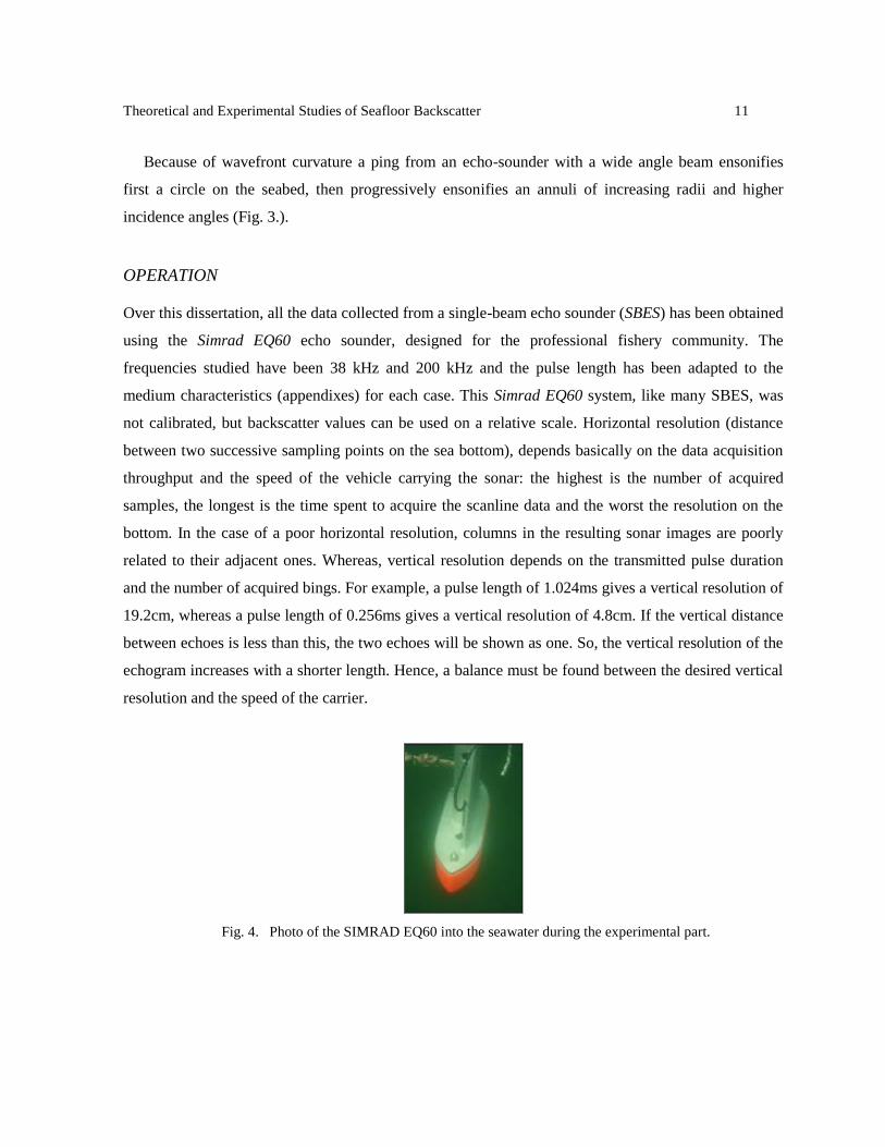
Fig. 4. Photo of the SIMRAD EQ60 into the seawater during the experimental part.

12 Theoretical and Experimental Studies of Seafloor Backscatter
ACOUSTIC SEAFLOOR CLASSIFICATION
The backscatter envelope recorded by SBESs represents the variation of amplitude with time, which
also relates to the angle of incidence. Hence, there are a variety of parameters derived from backscatter
envelope recorded by SBES that have found to be useful in seafloor classification [e.g. 5, 8, 12, 28].
Commonly used parameters include the backscatter strength based on the energy and intensity of the
seafloor envelope [28], which are referred to in this study as the surface scatting coefficient based on
energy (SSCE) and the surface scatting coefficient based on intensity (SSCI). Also, the energy of the
tail of the seafloor envelope (Fig. 5), referred to as E1 [ref - Chivers et al 1990], has been found by
many authors to be a very useful in discriminating different seafloor habitats as it ignores the
contributions from specular refection. More recently, [8] found the effective pulse width (EPW) was
useful for identifying areas of vegetated seafloor, such as seagrass.
Fig. 5. The parts of the first and second bottom returns. Energy of the shaded regions is integrated to form two
indices - E1 (for the tail of the first echo – summation begins one pulse length from the echo start) and E2 (for all
the second echo). From Hamilton (2001).
In this study, the different seafloor parameters are evaluated for their ability to discriminate
different seafloor habitats. The first part of the investigation is to use a SBES model to investigate the
relationship between these SBES parameters and depth, transmitted pulse width and the backscatter
coefficient of the seafloor (Chapter 3). Then SBES data collected from different seafloor habitats area
analysed to determine their ability to discriminate different seafloor habitats (Chapter 4). In Chapter 4

Theoretical and Experimental Studies of Seafloor Backscatter 13
uses comparison with towed video data, the Fisher Criterion, and Probability Distribution Function
(PDF) to help evaluate the different SBES parameters.
Underwater video analysis of coincident sections of the same SBES transect (using the head,
latitude, longitude), connected simultaneously to a GPS unit was carried out. The classification of the
habitats from the video is done by eye, visualizing and noting the seafloor sediment type along the
transect for each frame number to correlate to a position.
The Fisher Criterion is the distance between the means of the two classes normalised for the
variance within each class:
2
2
2
1
2
21)(
ss
mmwJ (5)
where m represents the mean, s2 represents the variance, and the subscripts denote the two classes.
The higher the Fisher Criterion the more separated the classes, the value has to be greater than 1 for
any class separation.
PDFs are a function that describes the relative likelihood for this random variable to occur at a
given point in the observation space. The probability of a random variable falling within a given set is
given by the integral of its density over the set. It is also useful to plot the probability of false alarm (1-
CDF) in a logarithmic scale to see the trend in the tail. PFA plots are used in Chapters 4 and 5 for
understanding the underlying scattering processes. For instance, Gaussian scattering will result in the
variation of SSCE to be well modelled by a Gamma distribution.
14 Theoretical and Experimental Studies of Seafloor Backscatter
III. MODELING SINGLE BEAM ECHO SOUNDER BACKSCATTER
1. INTRODUCTION
The aim of this chapter is to use a theoretical model developed by the CMST to predict the backscatter
envelope received by single beam echo sounders (Gavrilov, 2008) from different kinds of sediments, in
order to evaluate different parameters [45] used for seafloor classification. The single beam backscatter
characteristics studied in this dissertation were:
- Surface Scattering Coefficient derived from the backscatter Energy (SSCE).
- Surface Scattering Coefficient derived from the backscatter Intensity (SSCI).
- Backscatter energy in the tail of the echo signal (E1) [17] and Effective Pulse Width (EPW)
of backscatter envelope, which have been found to be important for seafloor classification
in other related studies [8].
These characteristics were calculated for the backscatter envelope predicted numerically from the
CMST model for different seafloor types. The surface scattering coefficient (or seafloor backscatter
strength) derived from these backscatter characteristics was then compared to the values used as input
parameters in the envelope model to evaluate the ability of measured backscatter characteristics to
discriminate different seafloor types. Previous studies have found that certain single beam parameters
can be dependent on depth and pulse width, e.g. E1 (Kloser et al, 2001). So, parameters calculated
from the envelope, were also tested to see if there was any dependence on sea depth or pulse width.
2. MODEL DESCRIPTION
The model used in this study is part of a suit of algorithms developed by CMST for the purpose of
investigating interference between different sonar systems deployed from the same platform and
operated at the same time (Gavrilov, 2008). A detailed description of the CMST model is given in
Gavrilov (2008), below is a summary.
The algorithm developed by CMST uses the Applied Physics Laboratory (APL) model [34] to
predict the seafloor backscatter coefficient based on seafloor properties. Ten types of sediments were
modelled; rough rock, rock, gravel, very coarse sand, coarse sand, medium sand, fine sand, very fine
sand, silt and clay. Very fine sediments composed mostly of clay are often “slow”, which means that
sound is refracted downward toward the vertical. Sound incident on a “fast” sediment is refracted
toward the horizontal and tends to penetrate to a lesser depth. The backscattering model is very
sensitive to the spatial spectrum of the surface roughness for coarser sediments and becomes less
Theoretical and Experimental Studies of Seafloor Backscatter 15
sensitive for finer sediments. Parameters linked to the sediment roughness are interpolated in the APL
method, and there exists a strong correlation between the sediment type and its roughness
characteristics. The bottom backscattering strength (Eq.6) is a sum of surface and volume components
and is a function of the bottom parameters: density, sound speed, sound attenuation, spectral exponent
and spectral strength of the surface roughness, volume inhomogeneity spectrum and some others. It is
also dependent on acoustic frequency and grazing angle.
)(log10 10 volumesurfacebS (6)
There is strong correlation between the energy and intensity of backscatter and the backscatter
coefficient volumesurface (Fig. 7). The surface roughness component ( surface ) of the
backscatter coefficient is evaluated as an input parameter for the envelope model. The volume
scattering component ( volume ) was set to zero to simplify calculations because its contribution at
vertical incidence of SBES is much smaller than that of the surface component (Gavrilov, 2008).
The model characteristics were chosen similar to those used in the experimental work, e.g. Simrad
EQ60 sonar parameters and settings and environmental characteristics. The input parameters used in
the algorithm are explained below:
Frequency of the transducer, which was 200 kHz in this study. Although measurements with the
38 kHz transducer were also taken, the 200-kHz backscatter data appeared to be much more
useful for the purposes of seafloor classification [8].
Pulse length: Simrad EQ60 transmits signal between 100 and 1024μs long. Several values were
tested.
Sediment properties, such as mean grain size, porosity, ratio between sediment and water
density, velocity and absorption and surface roughness spectrum [34]. Physical characteristics
of the water column, such as the sound speed in water and sea depth.
Measurement conditions, such as the location of the transducer (depth), sampling frequency.
Range to the bottom: varying from 5 m to 50 m. Depth dependence analysis is needed to
examine how envelopes evolve with increasing range.
Evaluation of the seafloor scattering coefficient involves numerous equations, beginning with the
roughness scattering component modelled with three different approximations (Kirchhoff, Composite
Roughness and Large-Roughness Scattering approximations applied in different angular domains[34]),
and ending with the sediment volume scattering coefficient. The resulting seafloor scattering
16 Theoretical and Experimental Studies of Seafloor Backscatter
coefficient is found as a function of incidence angle by interpolating results obtained in different
angular domains.
3. CORRELATION OF SINGLE BEAM BACKSCATTER CHARACTERISTICS WITH THE
SEAFLOOR BACKSCATTER COEFFICIENT
There are several parameters that can be derived from single beam backscatter envelopes, but to be
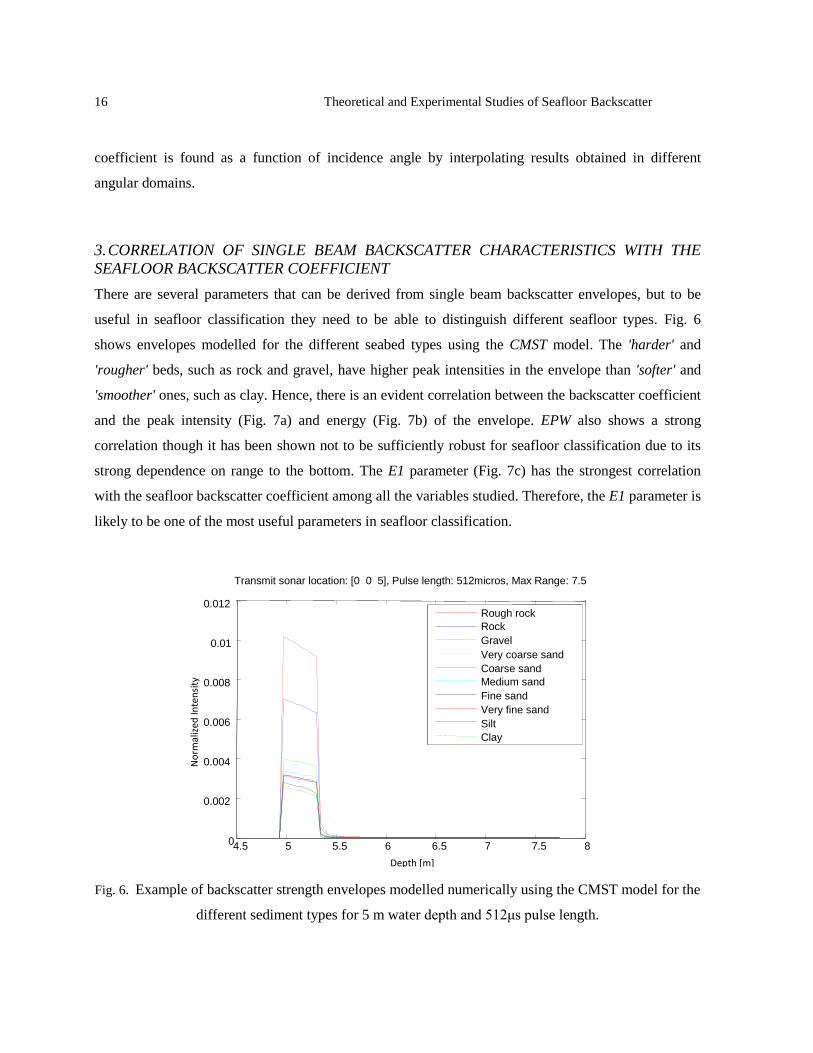
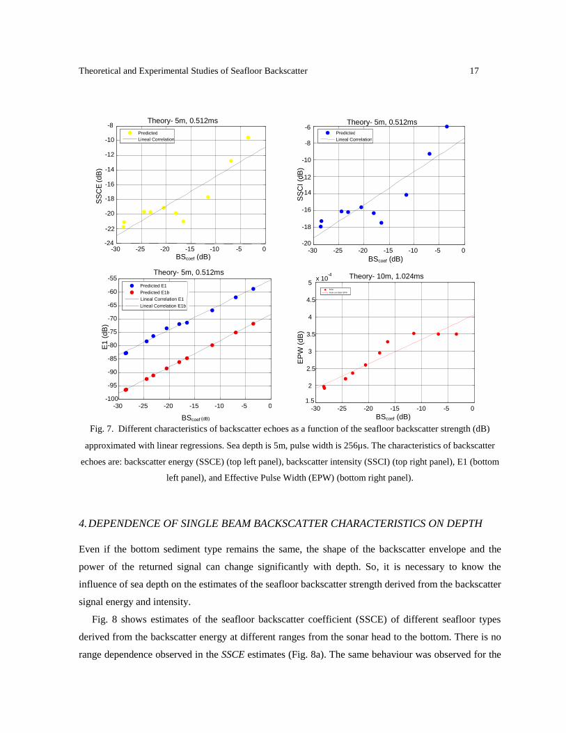
useful in seafloor classification they need to be able to distinguish different seafloor types. Fig. 6
shows envelopes modelled for the different seabed types using the CMST model. The 'harder' and
'rougher' beds, such as rock and gravel, have higher peak intensities in the envelope than 'softer' and
'smoother' ones, such as clay. Hence, there is an evident correlation between the backscatter coefficient
and the peak intensity (Fig. 7a) and energy (Fig. 7b) of the envelope. EPW also shows a strong
correlation though it has been shown not to be sufficiently robust for seafloor classification due to its
strong dependence on range to the bottom. The E1 parameter (Fig. 7c) has the strongest correlation
with the seafloor backscatter coefficient among all the variables studied. Therefore, the E1 parameter is
likely to be one of the most useful parameters in seafloor classification.
4.5 5 5.5 6 6.5 7 7.5 8 0
0.002
0.004
0.006
0.008
0.01
0.012
Transmit sonar location: [0 0 5], Pulse length: 512micros, Max Range: 7.5
Gravel
Very coarse sand
Fine sand
Very fine sand
Rough rock Rock
Coarse sand Medium sand
Silt
Clay
Depth [m]
No
rmal
ized
Inte
nsi
ty
Fig. 6. Example of backscatter strength envelopes modelled numerically using the CMST model for the
different sediment types for 5 m water depth and 512μs pulse length.
Theoretical and Experimental Studies of Seafloor Backscatter 17
a) b)
SS
CI (d
B)
-30 -25 -20 -15 -10 -5 0
Theory- 5m, 0.512ms
BScoef (dB)
Predicted Lineal Correlation
-30 -25 -20 -15 -10 -5 0
-22
-20
-18
-16
-14
-12
-10
-8 Theory- 5m, 0.512ms
BScoef (dB)
SS
CE
(dB
)
-24
Predicted Lineal Correlation
-6
-8
-10
-12
-14
-16
-18
-20
c) d)
-30 -25 -20 -15 -10 -5 0 -100
-95
-90
-85
-80
-75
-70
-65
-60
-55 Theory- 5m, 0.512ms
BScoef (dB)
E1 (
dB
)
Predicted E1
Lineal Correlation E1 Predicted E1b
Lineal Correlation E1b
-30 -25 -20 -15 -10 -5 0 1.5
2
2.5
3
3.5
4
4.5
5 x 10
-4
BScoef (dB)
EP
W (
dB
)
Theory- 10m, 1.024ms
EPW lineal correlation EPW
Fig. 7. Different characteristics of backscatter echoes as a function of the seafloor backscatter strength (dB)
approximated with linear regressions. Sea depth is 5m, pulse width is 256 s. The characteristics of backscatter
echoes are: backscatter energy (SSCE) (top left panel), backscatter intensity (SSCI) (top right panel), E1 (bottom
left panel), and Effective Pulse Width (EPW) (bottom right panel).
4. DEPENDENCE OF SINGLE BEAM BACKSCATTER CHARACTERISTICS ON DEPTH
Even if the bottom sediment type remains the same, the shape of the backscatter envelope and the
power of the returned signal can change significantly with depth. So, it is necessary to know the
influence of sea depth on the estimates of the seafloor backscatter strength derived from the backscatter
signal energy and intensity.
Fig. 8 shows estimates of the seafloor backscatter coefficient (SSCE) of different seafloor types
derived from the backscatter energy at different ranges from the sonar head to the bottom. There is no
range dependence observed in the SSCE estimates (Fig. 8a). The same behaviour was observed for the

18 Theoretical and Experimental Studies of Seafloor Backscatter
seafloor backscatter coefficient estimates from the backscatter intensity (SSCI). However, the range
dependence is significant for E1 (Fig. 8b) and so it is for the EPW. This means that changes in the sea
will affect estimates of the seafloor backscatter coefficient and, hence, results of acoustic classification
of the seafloor.
Fig. 8. a) SSCE estimates for different sediments made for a transmitted pulse of 256 µs long for
different sea depth from 10 to 35 m b) Estimates of parameter E1 made for the same pusle length,
ranges to the bottom and sediments.
Although E1 was found to be most correlated with the seafloor backscatter strength at a fixed range to
the bottom, it is not the best parameter for seafloor classification because of its significant dependence
on sea depth. For instance, the value of E1 for clay at a certain depth is similar to that of sand at a
shallower depth (Fig. 8b). Therefore, the E1 parameter needs to be properly corrected for sea depth
before it is used for seafloor classification. The cause of the depth dependence in E1 was found to be
an inadequate correction for insonification area. In the original algorithm [45], E1 is normalised by the
10 15 20 25 30 35 -18
-16
-14
-12
-10
-8
-6
-4 Pulse length: 256ms - Sample frequency = 50kHz
Depth (m)
SS
CE
(dB
)
10 15 20 25 30 35 -30
-28
-26
-24
-22
-20
-18
-16
-14
-12 Pulse length: 256ms - Sample frequency = 50kHz
Depth (m)
E1 (
dB
)
Very fine sand
Clay
Rough Rock
Rock
Gravel
Very Coarse sand
Coarse sand
Medium sand
Silt
Fine sand

Theoretical and Experimental Studies of Seafloor Backscatter 19
footprint area. However, the backscatter envelope in the echo tail is not correlated to the footprint area,
but for the instantaneous insonification area. The new algorithm for integration of the echo tail, which
makes correction for the insonification area rather than the footprint area, results in a different
parameter called E1b to distinguish it from the original E1parameter. This new parameter E1b corrected
properly for insonification area is no longer dependent on sea depth (Fig. 9).
Fig. 9. Energy of the bottom echo tail corrected the insonification area (E1b ) calculated for a transmitted pulse
of 256 µs long at different sea depth from 10 to 35m for different sediments.
5. DEPENDENCE OF SINGLE BEAM BACKSCATTER CHARACTERISTICS ON PULSE
WIDTH
If sea depth is not changing but the transmitted pulse length, the seafloor backscatter coefficient
derived from the energy and intensity of backscattered signals shows rather negligible dependence on
the pulse length. This was expected as the backscatter energy is normalised for pulse length, and the
peak intensity is normalized by the insonification area, which takes into account the range from the
sonar head to the seafloor. The E1parameter was found to have some dependence on pulse length.
However, the E1b parameter, which is corrected for insonification area, shows negligibly small
variations with pulse length (Fig. 10).
10 15 20 25 30 35 -20
-15
-10
-5 Pulse length: 256 ms - Sample frequency = 50 kHz
Depth (m)
E1
b (
dB
)
Very fine sand
Clay
Rough Rock
Rock
Gravel
Very Coarse sand
Coarse sand
Medium sand
Silt
Fine sand

20 Theoretical and Experimental Studies of Seafloor Backscatter
1200 -20
-15
-10
-5
pw (ms)
E1 b
(dB
)
0 200 400 600 800 1000
Depth: 10m - Sample frequency = 50 kHz
Very fine sand
Clay
Rough Rock
Rock
Gravel
Very Coarse sand
Coarse sand
Medium sand
Silt
Fine sand
Fig. 10. Energy of the bottom echo tail from different sediments corrected the insonification area (E1b )
calculated for a sea depth of 10 m and transmitted pulse length varying from 64 to 1024 µs.
6. DISCUSSION
The dependence of estimates of the seafloor backscatter strength, derived from different characteristics
of the backscatter envelope measured by SBES, on sea depth and transmitted pulse length was
examined in order to determine the most robust SBES backscatter characteristics to be use for seafloor
classification. Some dependence on sea depth and pulse length was found for the E1 parameter, but a
modification of it, the E1b parameter corrected for the insonification area, appeared to be much less
dependent on sea depth, which makes it appropriate for seafloor classification over areas of varying
bathymetry.
1200 -20
-15
-10
-5
pw (ms)
E1
b(d
B)
0 200 400 600 800 1000
Depth: 10m - Sample frequency = 50 kHz
Very fine sand
Clay
Rough Rock
Rock
Gravel
Very Coarse sand
Coarse sand
Medium sand
Silt
Fine sand

Theoretical and Experimental Studies of Seafloor Backscatter 21
IV. MEASURING SINGLE BEAM BACKSCATTER CHARACTERISTICS FROM
DIFFERENT HABITATS
1. INTRODUCTION
SBES has shown to be a useful tool in seafloor habitat mapping (Sotheran, Foster-Smith and Davies,
1997). A variety of different parameters derived from SBES backscatter data have been shown to be
useful in distinguishing different seafloor types (bare sediment, seagrass, coral reef, muddy beds, etc.).
These parameters are the backscatter energy and instantaneous intensity, the effective pulse with and
the E1 parameter, characterising the seabed roughness (See Chapter 2 for more detail of these
parameters) .
The aim of this Chapter is to evaluate the ability of these different SBES parameters to discriminate
different seafloor habitats. This study was carried out using data collected with a SBES along two
different transects that crossed different seafloor habitats including seagrass, coral reef and sand. The
SBES data were processed using an algorithm developed by the Centre for Marine Science and
Technology (Parnum, 2009), which calculates the different backscatter parameters discussed above.
The Fisher criterion was used to assess the ability of the different SBES parameters to discriminate
different seafloor types. In addition, a statistical analysis of backscatter fluctuations was carried out to
further understand the backscatter processes from different seafloor habitats and, in particular, to
examine if the backscatter process is Gaussian. Details of the seafloor acoustic scattering theory and
backscatter statistics can be found in Chapter 2 (background). The SBES data processing techniques
adopted in this study provide an alternative to the commercially available bottom classifiers.
2. METHODS
DATA COLLECTION
A Simrad EQ60 single beam echosounder (SBES), operating at 38 and 200 kHz, was used to collect
seafloor backscatter from two different areas of Australia:
1. Owen Anchorage in Western Australia.
2. Morinda Shoal in Queensland, Australia .
SBES data were collected on 21st October 2005 in Owen Anchorage, which is a shallow water area
(<20 m) within Cockburn Sound, Perth, Western Australia. From the previous ground-truth
information, seagrass (Posidonia) was known to be present in the shallow eastern side of the transect;
22 Theoretical and Experimental Studies of Seafloor Backscatter
whereas, an unvegetated seabed composed mainly of sand and muddy sand was present in the deeper
western side of the transect [26].The transmit pulse duration used at 38 kHz and 200 kHz was 4096μs
and 1024μs respectively.
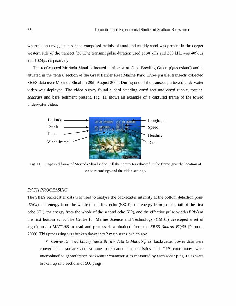
The reef-capped Morinda Shoal is located north-east of Cape Bowling Green (Queensland) and is
situated in the central section of the Great Barrier Reef Marine Park. Three parallel transects collected
SBES data over Morinda Shoal on 20th August 2004. During one of the transects, a towed underwater
video was deployed. The video survey found a hard standing coral reef and coral rubble, tropical
seagrass and bare sediment present. Fig. 11 shows an example of a captured frame of the towed
underwater video.
Fig. 11. Captured frame of Morinda Shoal video. All the parameters showed in the frame give the location of
video recordings and the video settings.
DATA PROCESSING
The SBES backscatter data was used to analyse the backscatter intensity at the bottom detection point
(SSCI), the energy from the whole of the first echo (SSCE), the energy from just the tail of the first
echo (E1), the energy from the whole of the second echo (E2), and the effective pulse width (EPW) of
the first bottom echo. The Centre for Marine Science and Technology (CMST) developed a set of
algorithms in MATLAB to read and process data obtained from the SBES Simrad EQ60 (Parnum,
2009). This processing was broken down into 2 main steps, which are:
Convert Simrad binary fileswith raw data to Matlab files: backscatter power data were
converted to surface and volume backscatter characteristics and GPS coordinates were
interpolated to georeference backscatter characteristics measured by each sonar ping. Files were
broken up into sections of 500 pings,
Heading
Depth
Time
Speed
Date Video frame
Longitude Latitude

Theoretical and Experimental Studies of Seafloor Backscatter 23
Main processing: The sections for each original file were recombined and processed to
calculate for each ping:
i. Depth (m), and
ii. Seafloor backscatter parameters (including E1 and E2)
More details on the seafloor backscatter parameters and the MATLAB SBES toolbox can be found
in the introduction and in Parnum (2009) respectively.
DATA ANALYSIS
The seafloor backscatter characteristics derived from the SBES data were grided into 100 m cells to
analyse along track changes. Probability density functions (PDFs) of variations in backscatter
characteristics and a Fisher criterion for distinguishing different distributions for different seafloor
habitats were calculated to assess the ability of the different characteristics to discriminate different
seafloor types. The Probability of False Alarm (PFA) was calculated for normalised values of
backscatter energy to assess whether the scattering processes from the different seafloor habitats could
be modelled by a number of selected model distributions, including those for a Gaussian process.
3. RESULTS
OWEN ANCHORAGE - SBES DEPTH AND BACKSCATTER PARAMETERS
Fig. 12 shows the sea depth along the two parallel transects across the Owen Anchorage survey area.
The backscatter characteristics E1, SSCE, SSCI and EPW measured at 200 kHz along these transects
are shown in Fig. 13. At 38 kHz, there was a little difference between the distributions of the
backscatter parameters measured from different habitats. However, the difference in the distributions at
200 kHz is noticeable and, therefore, the backscatter characteristics at 200 kHz were used for seafloor
classification. The discrimination of two different habitats with the E1 parameter at 200 kHz is quite
good, as shown in Fig. 14. The SSCE parameter also provides reasonable discrimination. Apparently,
SSCI appeared not to be a good parameter for this purpose, neither the EPW, as also seen in Fig.14
Table 1 gives the Fisher criterion for the different SBES parameters at 200 kHz. The SSCE and E1
parameters at 200 kHz both have values greater than unity.

24 Theoretical and Experimental Studies of Seafloor Backscatter
0 500 1000 15006
7
8
9
10
11
12
13
14
15
Depth from Transect L54
38kHz200kHz
Dep
th(m
)
Distance (m)
Fig. 12. Depth calculated from the sonar data at 38 kHz and 200 kHz.
0 200 400 600 800 1000 1200 1400 1600 1800-110
-108
-106
-104
-102
-100
-98
-96
-94
Meters
Me
an
Va
lue
n=100m - nBoxes=19 - F=200 kHz - E1
L0055
L0056
-94
-93
-92
-91
-90
-89
-88
-87n=100m - nBoxes=19 - F=200 kHz - SSCE
L0055
L0056
-100
-99
-98
-97
-96
-95
-94
-93
-92
-91
-90
Me
an
Va
lue
n=100m - nBoxes=19 - F=200 kHz - SSCI
L0055
L0056
2.2
2.4
2.6
2.8
3
3.2
3.4
3.6
3.8
Me
an
Va
lue
n=100m - nBoxes=19 - F=200 kHz - EPW
L0055
L0056
0 200 400 600 800 1000 1200 1400 1600Meters
Mean V
alu
e
0 200 400 600 800 1000 1200 1400 1600Meters
0 200 400 600 800 1000 1200 1400 1600Meters
Fig. 13. Backscatter characteristics at 200 kHz averaged over 100-m sections of transects: E1 (top left), SSCE
(top right), SSCI (bottom left) and EPW (bottom right)

Theoretical and Experimental Studies of Seafloor Backscatter 25
Fisher Criterion E1 SSCE SSCI
Transect L055 L056 L055 L056 L055 L056
Linear Data 1.824233 1.615829 0.167947 0.282942 0.747347 0.245258
Table 1. Fisher criterion for each interested backscatter parameter.
-115 -110 -105 -100 -95 -90 -85
0.02
0.04
0.06
0.08
0.1
0.12
Density Function Backscatter - E1
Seagrass L055 Sand L055 Seagrass L056 Sand L056
No
rmal
ized
En
ergy
PD
F
Energy (dB)dB
PD
F
dB -100 -95 -90 -85 -80
0.02
0.04
0.06
0.08
0.1
0.12
0.14
0.16
Density Function Backscatter - SSCE
Seagrass L055 Sand L055 Seagrass L056 Sand L056
No
rmal
ized
En
ergy
-110 -105 -100 -95 -90 -85 -80
0.02
0.04
0.06
0.08
0.1
0.12
Density Function Backscatter - SSCI
Seagrass L055 Sand L055 Seagrass L056 Sand L056
No
rmal
ized I
nte
nsi
ty
PD
F
dB
Fig. 14. Probability Density Function of variations of three different backscatter characteristics measured over
sand (blue) and seagrass (green) areas along two transects in Owen Anchorage: E1(top left panel ), SSCE (top
right panel ), and SSCI (bottom panel).

26 Theoretical and Experimental Studies of Seafloor Backscatter
MORINDA SHOAL - SBES DEPTH AND BACKSCATTER PARAMETERS
Fig. 15 shows the sea depth along the SBES transects over the Morinda Shoal survey area. Variations
of the four measured backscatter characteristics SSCE, E1, SSCI and EPW along these transects and
results of visual classification of the seafloor based on using video recordings are shown in Fig. 17.
-5.6765-5.676 -5.6755-5.675 -5.6745-5.674 -5.6735-5.673 -5.6725
x 106
5.5
5.5005
5.501
5.5015
5.502
5.5025
5.503
x 106
Easting
Nort
hin
g
Transects Single Beam Morinda Shoal Depth
15
20
25
30
35
40
Fig. 15. Sea depth along SBES transects over the Morinda Shoal survey area.
Fig. 16. Video captures of three different seafloor types found in the Morinda Shoal area: Coral(left), Rock
(middle) and Seagrass (right)
The probability density functions of the measured backscatter characteristic show obvious
discrimination between three different habitats (Fig. 18). According to Fig. 18, the parameters of best
seafloor discrimination are SSCE and E1. Three separate peaks can be easily distinguished in the PDFs
of SSCE and E1, which are related to the three different type of bottom observed in the video footage
taken along the transects in Morinda Shoal (Fig.16).

Theoretical and Experimental Studies of Seafloor Backscatter 27
0 500 1000 1500 2000 2500-95
-90
-85SSCE
0 500 1000 1500 2000 2500-95
-90
-85E1
0 500 1000 1500 2000 2500-110
-100
-90SSCI
0 500 1000 1500 2000 25000.2
0.3
0.4
0.5EPW
0 500 1000 1500 2000 2500
2
4
6Video
dB
dB
dB
Tim
e(s
)B
ott
om
typ
es
Distance (m)
Distance (m)
Distance (m)
Distance (m)
Distance (m)
Fig. 17. Four different backscatter characteristics measured at 200 kHz along the SBES transects in Morinda
Shoal (panels 1 to 4 from top: SSCE, E1, SSCI and EPW) and visual classification of the seafloor from video
(bottom panel). The classification numbers correspond to different seafloor types as follows: 1 - Coral, 2. - Coral-
Rock, 3 - Rock, 4 - Gravel, 5 - Seagrass (Low density), 6 - Seagrass (High density).
Coral Seagrass
Rock

28 Theoretical and Experimental Studies of Seafloor Backscatter
dB
-96 -94 -92 -90 -88 -86 -840
0. 05
0. 1
0. 15
0. 2
0. 25
0. 3
0. 35M or i nda S hoa l E 1200
-93 -92 -91 -90 -89 -88 -87 -86 -85 -84 -830
0. 05
0. 1
0. 15
0. 2
0. 25
0. 3
0. 35
0. 4M or i nda S hoa l S S CE 200
-110 -105 -100 -95 -90 -850
0. 05
0. 1
0. 15
0. 2
0. 25
0. 3
0. 35
0. 4
0. 45M or i nda S hoa l S S CI200
0. 2 0. 25 0. 3 0. 35 0. 4 0. 450
5
10
15
20
25M or i nda S hoa l E P W 200
Time (s)
dB dB
Fig. 18. Normalized distributions of four backscatter characteristics measured in Morinda Shoal: E1(top left),
SSCE (top right), SSCI (bottomleft) and EPW (bottom right).
ANALYSIS OF THE DISTRIBUTION FUNCTION - OWEN ANCHORAGE
The PFA of the normalized backscatter intensity (SSCI) and energy (SSCE) for selected habitats is
shown in Fig. 19 for 38 kHz (top panels) and 200 kHz (bottom panels). The aim of this analysis is to
examine whether the scattering process is Gaussian or non-Gaussian. Gaussian scattering would cause
variations of SSCE to be Gamma distributed and SSCI to be exponentially distributed. The PFA
assesses the tail of a distribution, whereas PDFs assesses the shape of a distribution [21].
For the 38 kHz data from sand, the experimental distributions do not fit well any model distribution
and seem to be closer to the Gamma distribution (Fig. 19 top). The distributions at 200 kHz can be
reasonably well approximated by a Gamma model (Fig. 19 bottom)

Theoretical and Experimental Studies of Seafloor Backscatter 29
0 2 4 6 8 10 12 1410
-8
10-7
10-6
10-5
10-4
10-3
10-2
10-1
100
Data
FA
FA normbsSSCE - Data Line 055, Sand, 38kHz
Data
Rayleigh model
Exponential
LogNormal
Gamma
Weibul
0 0.5 1 1.5 2 2.5 3 3.5 410
-5
10-4
10-3
10-2
10-1
100
Data
FA
FA normbsSSCE - Data Line 055, Seagrass, 38kHz
Data
Rayleigh model
Exponential
LogNormal
Gamma
Weibul
0 0.5 1 1.5 2 2.5 3
10 -4
10 -3
10 -2
10 -1
10 0
Data
FA
FA normbsSSCE - Data Line 055, 200kHz
Data
Rayleigh model
Exponential
LogNormal
Gamma
Weibul
0 0.5 1 1.5 2 2.5 3 3.5 4
10 -4
10 -3
10 -2
10 -1
10 0
Data
FA
FA normbsSSCE - Data Line 055, 200kHz
Data
Rayleigh model
Exponential
LogNormal
Gamma
Weibul
Fig. 19. PFAs of the SSCE backscatter characteristic measured from sand (left panels) and seagrass (right
panels) at 38 kHz (top panels) and 200 kHz (bottom panels) in Owen Anchorage
4. CONCLUSIONS
The E1 and SSCE backscatter parameters measured at 200 kHz were the most robust for discriminating
different seafloor habitats.
Seafloor classification based on these parameters was able to discriminate sand and seagrass in
Owen Anchorage, and also more complex seafloor types, such as coral, found in Morinda Shoal.
Variations of the backscatter energy (SSCE) at 200 kHz observed from sand and seagrass were well
approximated by the Gamma distribution, which suggests the scattering process to be nearly Gaussian.

30 Theoretical and Experimental Studies of Seafloor Backscatter
V. TEMPORAL VARIABILITY OF SINGLE BEAM ECHO SOUNDER
1. INTRODUCTION
Previous studies [12][46] have shown that acoustic backscatter from seagrass is comparable to, or even
stronger than that from surroundings areas of unvegetated seafloor. The physical mechanisms driving
the higher backscatter from seagrass are poorly understood. Laboratory experiments have shown the
sound speed in a plant-filled resonator to be dependent on plant biomass and tissue characteristics,
which varies for different seagrass species [47]. In addition, the acoustic response from seagrass is
influenced by photosynthetic activity which produces gas bubbles on the plants and in the water
column [48]. However, it is unknown how much backscatter measured from seagrass is due to plant
material, including air filled tissues, and how much of it might be due to microbubbles of gas produced
by photosynthesis and/or respiration processes. If bubbles produced by gas emission are a significant
contributor to the acoustic backscatter strength, then the backscatter intensity from seagrass could
potentially change as the rate of gas production varies over the course of the day and season. Such
variations, if they are significant, could seriously affect seagrass mapping by acoustic means. Gas
bubbles released from seagrass due to photosynthesis and/or respiration are one of the most likely
sources of strong scattering. If this is so, then the backscatter level from seagrass could vary with time,
as the rate of gas emission changes during the day and in different seasons due to changes in the sun
illumination. Using a Simrad EQ60 single beam echosounder deployed from a jetty on Garden Island
in Western Australia, acoustic backscatter from an area of dense seagrass Posidonea was measured at
38 kHz and 200 kHz every 2 s over 7 days. This study investigated the temporal variability of
backscatter from an area of dense seagrass (Posidonia) measured at 38 kHz and 200 kHz using a single
beam echosounder over a long time period (7 days).
2. METHODS
Acoustic backscatter from seagrass was measured between 2nd and 8th March 2010 using a dual-
frequency Simrad EQ60 single-beam echosounder, which was fixed to a jetty on Garden Island in
Western Australia. The distance from the transducer head to the sediment-water interface was fixed at
about 3.1 m over the whole measurement period. The transducer depth was about 1 m at the start of
measurements and varied with tide by less than 1 m during the experiment. Backscatter echoes were
collected every 2 s at both 38 and 200 kHz for seven days. The sonar pulse length was 512 µs at 38
kHz and 100 µs at 200 kHz.

Theoretical and Experimental Studies of Seafloor Backscatter 31
The backscatter energy of the primary bottom echo and the instantaneous intensity at the bottom
detection time were measured to analyse long-term variations and statistics of short-term fluctuations.
The surface scattering coefficient was not calculated, because the echo sounder was not adequately
calibrated with respect to transmitted power and receives gain. So, the backscatter intensity values are
represented below in relative units. All sonar setting, such as transmitted power and pulse length were
kept the same during the experiment to simplify comparison of backscatter measurements from
seagrass and the surrounding areas of bare sediment.
Seagrass leaves are almost always moving under variable local currents due to tides and surface
waves, which leads to significant and relatively fast fluctuations of the backscatter intensity measured
from the same area of seagrass. A correlation analysis was used to select statistically independent
samples of backscatter from seagrass for which the probability density function (PDF) and probability
of false alarm (PFA) of backscatter characteristics were calculated and compared with the most typical
statistical models associated with seafloor acoustic backscatter, such as Rayleigh, Gamma, K-
distribution and lognormal models [49]
To compare backscatter from seagrass and bare sediments at the same frequencies, additional short-
term measurements were made over an area of unvegetated muddy sand located about 10 m away from
the seagrass measurement site at about the same sea depth.
3. BACKSCATTER FROM SEAGRASS AND ITS LONG-TERM VARIATIONS
0shows the level of backscatter intensity at 200 kHz and 38 kHz as a function of range from the sonar
head to the bottom covered with seagrass and bare sand. Because the sea depth at the seagrass and sand
sites was slightly different, the echoes from sand shown in 0 are aligned with those from seagrass at the
bottom range.

32 Theoretical and Experimental Studies of Seafloor Backscatter
2 2.5 3 3.5 4 4.5 5 5.5 6-100
-90
-80
-70
-60
-50
-40
-30
Range, m
Re
lative
backscatt
er
leve
l, d
B
38kHz, pulse length 512 s, power - 100W
2 2.5 3 3.5 4 4.5 5 5.5 6-140
-130
-120
-110
-100
-90
-80
-70
-60
-50
-40
Re
lative
backscatt
er
leve
l, d
B
200kHz, pulse length 100 s, power 100W
Range to bottom~30cm
Seagrass
Sand
2 2.5 3 3.5 4 4.5 5 5.5 6-100
-90
-80
-70
-60
-50
-40
-30
Range, m
Rela
tive
backscatt
er
leve
l, d
B
38kHz, pulse length 512 s, power - 100W
2 2.5 3 3.5 4 4.5 5 5.5 6-140
-130
-120
-110
-100
-90
-80
-70
-60
-50
-40
Rela
tive
backscatt
er
leve
l, d
B
200kHz, pulse length 100 s, power 100W
Range to bottom~30cm
Seagrass
Sand
Fig. 20. Backscatter intensity level of the primary bottom echo from seagrass (green) and bare sand (red)
averaged over 200 pings at 200 kHz (left) and 38 kHz (right).
The maximum amplitude of the mean envelope at 200 kHz is approximately the same for seagrass
and sand. However, the backscatter signal recorded from the seagrass is stronger than bare sand both
before and after the bottom detection range. The higher backscatter from the seagrass before the
bottom detection point is the acoustic energy backscattered from the seagrass canopy and forms a less
abrupt leading edge. The range to the leading edge of the echo from seagrass indicates that the canopy
height was about 30 cm. The higher backscatter from seagrass (relative to bare sand) after the bottom
detection point means that the backscatter strength of seagrass at oblique angles of incidence within the
sonar beam is significantly stronger than that of bare sand. At 38 kHz, the effect of seagrass on
backscatter echoes is similar but less pronounced.
2 2.5 3 3.5 4 4.5 5 5.5 6-100
-90
-80
-70
-60
-50
-40
-30
Range, m
Rela
tive
backscatt
er
leve
l, d
B
38kHz, pulse length 512 s, power - 100W
2 2.5 3 3.5 4 4.5 5 5.5 6-140
-130
-120
-110
-100
-90
-80
-70
-60
-50
-40
Rela
tive
backscatt
er
leve
l, d
B
200kHz, pulse length 100 s, power 100W
Range to bottom~30cm
Seagrass
Sand
2 2.5 3 3.5 4 4.5 5 5.5 6-100
-90
-80
-70
-60
-50
-40
-30
Range, m
Rela
tive
backscatt
er
leve
l, d
B
38kHz, pulse length 512 s, power - 100W
2 2.5 3 3.5 4 4.5 5 5.5 6-140
-130
-120
-110
-100
-90
-80
-70
-60
-50
-40
Re
lative
backscatt
er
leve
l, d
B
200kHz, pulse length 100 s, power 100W
Range to bottom~30cm
Seagrass
Sand
2 2.5 3 3.5 4 4.5 5 5.5 6-100
-90
-80
-70
-60
-50
-40
-30
Range, m
Rela
tive
backscatt
er
leve
l, d
B
38kHz, pulse length 512 s, power - 100W
2 2.5 3 3.5 4 4.5 5 5.5 6-140
-130
-120
-110
-100
-90
-80
-70
-60
-50
-40
Re
lative
backscatt
er
leve
l, d
B
200kHz, pulse length 100 s, power 100W
Range to bottom~30cm
Seagrass
Sand
Theoretical and Experimental Studies of Seafloor Backscatter 33
1
2
3
4
38 kHz
200 kHz
1
2
3
4
38 kHz
200 kHz
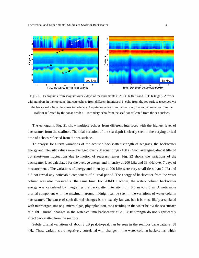
Fig. 21. Echograms from seagrass over 7 days of measurements at 200 kHz (left) and 38 kHz (right). Arrows
with numbers in the top panel indicate echoes from different interfaces: 1- echo from the sea surface (received via
the backward lobe of the sonar transducer); 2 – primary echo from the seafloor; 3 – secondary echo from the
seafloor reflected by the sonar head; 4 – secondary echo from the seafloor reflected from the sea surface.
The echograms Fig. 21 show multiple echoes from different interfaces with the highest level of
backscatter from the seafloor. The tidal variation of the sea depth is clearly seen in the varying arrival
time of echoes reflected from the sea surface.
To analyse long-term variations of the acoustic backscatter strength of seagrass, the backscatter
energy and intensity values were averaged over 200 sonar pings (400 s). Such averaging almost filtered
out short-term fluctuations due to motion of seagrass leaves. Fig. 22 shows the variations of the
backscatter level calculated for the average energy and intensity at 200 kHz and 38 kHz over 7 days of
measurements. The variations of energy and intensity at 200 kHz were very small (less than 2 dB) and
did not reveal any noticeable component of diurnal period. The energy of backscatter from the water
column was also measured at the same time. For 200-kHz echoes, the water- column backscatter
energy was calculated by integrating the backscatter intensity from 0.5 m to 2.5 m. A noticeable
diurnal component with the maximum around midnight can be seen in the variations of water-column
backscatter. The cause of such diurnal changes is not exactly known, but it is most likely associated
with microorganisms (e.g. micro-algae, phytoplankton, etc.) residing in the water below the sea surface
at night. Diurnal changes in the water-column backscatter at 200 kHz strength do not significantly
affect backscatter from the seafloor.
Subtle diurnal variations of about 3 dB peak-to-peak can be seen in the seafloor backscatter at 38
kHz. These variations are negatively correlated with changes in the water-column backscatter, which

34 Theoretical and Experimental Studies of Seafloor Backscatter
are, most likely, the major cause of seafloor backscatter variations at 38 kHz (in contrast to that at 200
kHz). The effect of water-column backscatter on the bottom echoes is clearly seen in Fig. 21. Strong
water-column backscatter was observed right before midnight of day 3, which was probably caused by
small fish schools appeared in the water at that time. This reduced considerably the energy of
backscatter from the seafloor, especially at 38 kHz.
200 kHz
-60
-55
-50
-45
-40
-35
Backscatt
er
level, d
B
0 2 4 6 8-60
-55
-50
-45
-40
-35
-30
-25
-20
Time, Day
Backscatt
er
level, d
B
38 kHz
200 kHz
-60
-55
-50
-45
-40
-35
Backscatt
er
level, d
B
0 2 4 6 8-60
-55
-50
-45
-40
-35
-30
-25
-20
Time, Day
Backscatt
er
level, d
B
0 2 4 6 8-60
-55
-50
-45
-40
-35
-30
-25
-20
Time, Day
Backscatt
er
level, d
B
38 kHz
200 kHz
-60
-55
-50
-45
-40
-35
Backscatt
er
level, d
B
0 2 4 6 8-60
-55
-50
-45
-40
-35
-30
-25
-20
Time, Day
Backscatt
er
level, d
B
38 kHz
200 kHz
-60
-55
-50
-45
-40
-35
Backscatt
er
level, d
B
0 2 4 6 8-60
-55
-50
-45
-40
-35
-30
-25
-20
Time, Day
Backscatt
er
level, d
B
0 2 4 6 8-60
-55
-50
-45
-40
-35
-30
-25
-20
Time, Day
Backscatt
er
level, d
B
38 kHz
Fig. 22. Variations of backscatter energy (red) and instantaneous intensity (green) from seagrass and water-
column backscatter energy (blue) observed at 200 kHz (left) and 38 kHz (right) over 7 days of measurements.
4. STATISTICAL ANALYSIS OF SHORT-TERM FLUCTUATIONS
To statistically analyse fluctuations of backscatter from seagrass, a data section of relatively stationary
fluctuations during days 3 – 6 (about 170,000 pings) was chosen. An autocorrelation function of
fluctuations was calculated at both frequencies to determine statistically independent samples of
backscatter characteristics. It appeared that the 2-s ping interval was long enough for the adjacent
samples of backscatter energy and intensity at 200 kHz not to be correlated, so that every sample could
be taken for statistical analysis. At 38 kHz, adjacent samples were correlated to some extent, so every
second sample was chosen for analysis.
A Probability Density Function (PDF) and Probability of False Alarm (PFA) were calculated for the
distributions of backscatter energy and intensity at 200 kHz and 38 kHz. The experimental
distributions of backscatter characteristics were compared with a number of model distributions which
either had some physical ground for the measured backscatter parameters or provided reasonably good
fits for backscatter data collected in previous experiments [21][49]. For the backscatter energy, the K-
distribution, Gamma ( ) and Lognormal models were tested, as the most appropriate ones. In addition,
200 kHz
-60
-55
-50
-45
-40
-35
Backscatt
er
level, d
B
0 2 4 6 8-60
-55
-50
-45
-40
-35
-30
-25
-20
Time, Day
Backscatt
er
level, d
B
38 kHz
200 kHz
-60
-55
-50
-45
-40
-35
Backscatt
er
level, d
B
0 2 4 6 8-60
-55
-50
-45
-40
-35
-30
-25
-20
Time, Day
Backscatt
er
level, d
B
0 2 4 6 8-60
-55
-50
-45
-40
-35
-30
-25
-20
Time, Day
Backscatt
er
level, d
B
38 kHz
200 kHz
-60
-55
-50
-45
-40
-35
Backscatt
er
level, d
B
0 2 4 6 8-60
-55
-50
-45
-40
-35
-30
-25
-20
Time, Day
Backscatt
er
level, d
B
38 kHz
200 kHz
-60
-55
-50
-45
-40
-35
Backscatt
er
level, d
B
0 2 4 6 8-60
-55
-50
-45
-40
-35
-30
-25
-20
Time, Day
Backscatt
er
level, d
B
0 2 4 6 8-60
-55
-50
-45
-40
-35
-30
-25
-20
Time, Day
Backscatt
er
level, d
B
38 kHz

Theoretical and Experimental Studies of Seafloor Backscatter 35
an extreme value distribution model was tested for the backscatter energy data. It has been shown
[50][51] that a sum of statistically independent backscatter intensity samples taken at different times of
the backscatter signal tends to be -distributed, if fluctuations of the backscatter envelop measured in
different pings (from different scattering patches) have Rayleigh statistics (or an exponential
distribution for intensity), i.e. when the backscatter process is Gaussian. A -like distribution is also
expected for the energy of processes that have other distributions of the instantaneous intensity, such as
the K-distribution, with the tail shape similar to that of the exponential distribution. The echo signal
from seagrass is relatively long for a short transmitted pulse of 100 µs (7.5 cm in terms of range
resolution), so one can expect that backscatter samples taken from the same echo at different arrival
times with intervals larger than 100 µs correspond to scattering from different parts (leaves and stems)
of the seagrass canopy. Consequently, fluctuations of those samples should not be correlated and the
variation of backscatter energy should tend to a -like distribution.
The PDF and PFA of backscatter energy from seagrass are shown in Fig. 23. The -distribution
model fits the experimental PDF reasonably well, but the tail of the -distribution is noticeably lighter
than that of the experimental distribution, which is clearly seen in the PFA behaviour. The lognormal
model provides a noticeably better fit for both most probable (i.e. PDF shape) and highest (i.e. PFA
slope) values of backscatter energy. Although this does not have any reasonable physical explanation,
some previous studies, e.g. [49][50], also showed a good fit of the lognormal model for backscatter
energy fluctuations.

36 Theoretical and Experimental Studies of Seafloor Backscatter
2 4 6 8 10 12
10-4
10-3
10-2
10-1
100
Normalized energy, rel.units
Pro
bab
ility
of
fals
e a
larm
38 kHz
Data
K-distrib.
Gamma
Lognormal
Exponential
Extreme
0 1 2 3 4 5 60
0.2
0.4
0.6
0.8
1
1.2
1.4
Normalized energy, rel.units
Pro
bab
ility
den
sity
38 kHz
Data
K-distrib.
Gamma
Lognormal
Exponential
Extreme
0 0.5 1 1.5 2 2.5 30
0.2
0.4
0.6
0.8
1
1.2
1.4
Normalized energy, rel.units
Pro
bab
ility
den
sity
200 kHz
Data
K-distrib.
Gamma
Lognormal
Extreme
1 2 3 4
10-4
10-3
10-2
10-1
100
Normalized energy, rel.units
Pro
bab
ility
of
fals
e a
larm
200 kHz
Data
K-distrib.
Gamma
Lognormal
Extreme
2 4 6 8 10 12
10-4
10-3
10-2
10-1
100
Normalized energy, rel.units
Pro
bab
ility
of
fals
e a
larm
38 kHz
Data
K-distrib.
Gamma
Lognormal
Exponential
Extreme
2 4 6 8 10 12
10-4
10-3
10-2
10-1
100
2 4 6 8 10 12
10-4
10-3
10-2
10-1
100
Normalized energy, rel.units
Pro
bab
ility
of
fals
e a
larm
38 kHz
Data
K-distrib.
Gamma
Lognormal
Exponential
Extreme
0 1 2 3 4 5 60
0.2
0.4
0.6
0.8
1
1.2
1.4
Normalized energy, rel.units
Pro
bab
ility
den
sity
38 kHz
Data
K-distrib.
Gamma
Lognormal
Exponential
Extreme
0 1 2 3 4 5 60
0.2
0.4
0.6
0.8
1
1.2
1.4
Normalized energy, rel.units
Pro
bab
ility
den
sity
38 kHz
Data
K-distrib.
Gamma
Lognormal
Exponential
Extreme
Data
K-distrib.
Gamma
Lognormal
Exponential
Extreme
0 0.5 1 1.5 2 2.5 30
0.2
0.4
0.6
0.8
1
1.2
1.4
Normalized energy, rel.units
Pro
bab
ility
den
sity
200 kHz
Data
K-distrib.
Gamma
Lognormal
Extreme
0 0.5 1 1.5 2 2.5 30
0.2
0.4
0.6
0.8
1
1.2
1.4
Normalized energy, rel.units
Pro
bab
ility
den
sity
200 kHz
Data
K-distrib.
Gamma
Lognormal
Extreme
1 2 3 4
10-4
10-3
10-2
10-1
100
Normalized energy, rel.units
Pro
bab
ility
of
fals
e a
larm
200 kHz
Data
K-distrib.
Gamma
Lognormal
Extreme
1 2 3 4
10-4
10-3
10-2
10-1
100
Normalized energy, rel.units
Pro
bab
ility
of
fals
e a
larm
200 kHz
Data
K-distrib.
Gamma
Lognormal
Extreme
Fig. 23. Probability density function (left panels) and probability of false alarm (right panels) of backscatter
energy fluctuations measured from seagrass at 200 kHz (top panels) and 38 kHz (bottom panels) shown with the
best fits of different distribution models.
0 1 2 30
0.2
0.4
0.6
0.8
1
1.2
1.4
Normalized envelope, rel.units
Pro
bab
ility
den
sity
38 kHz, Intanteneous envelope
Data
K-distrib.
Rayleigh
Rayleigh Mix 2
1 2 3 4
10-4
10-3
10-2
10-1
100
Normalized envelope, rel.units
Pro
bab
ility
of
fals
e a
larm
38 kHz, Intanteneous envelope
Data
K-distrib.
Rayleigh
Rayleigh Mix 2
0.5 1 1.5 2 2.5 3 3.5
10-4
10-3
10-2
10-1
100
Normalized envelope, rel.units
Pro
bab
ility
of
fals
e a
larm
200 kHz, Intanteneous envelope
Data
K-distrib.
Rayleigh
Rayleigh Mix 2
0 0.5 1 1.5 2 2.5 30
0.2
0.4
0.6
0.8
1
Normalized envelope, rel.units
Pro
bab
ility
den
sity
200 kHz, Intanteneous envelope
Data
K-distrib.
Rayleigh
Rayleigh Mix 2
0 1 2 30
0.2
0.4
0.6
0.8
1
1.2
1.4
Normalized envelope, rel.units
Pro
bab
ility
den
sity
38 kHz, Intanteneous envelope
Data
K-distrib.
Rayleigh
Rayleigh Mix 2
0 1 2 30
0.2
0.4
0.6
0.8
1
1.2
1.4
Normalized envelope, rel.units
Pro
bab
ility
den
sity
38 kHz, Intanteneous envelope
Data
K-distrib.
Rayleigh
Rayleigh Mix 2
1 2 3 4
10-4
10-3
10-2
10-1
100
Normalized envelope, rel.units
Pro
bab
ility
of
fals
e a
larm
38 kHz, Intanteneous envelope
Data
K-distrib.
Rayleigh
Rayleigh Mix 2
1 2 3 4
10-4
10-3
10-2
10-1
100
Normalized envelope, rel.units
Pro
bab
ility
of
fals
e a
larm
38 kHz, Intanteneous envelope
Data
K-distrib.
Rayleigh
Rayleigh Mix 2
0.5 1 1.5 2 2.5 3 3.5
10-4
10-3
10-2
10-1
100
Normalized envelope, rel.units
Pro
bab
ility
of
fals
e a
larm
200 kHz, Intanteneous envelope
Data
K-distrib.
Rayleigh
Rayleigh Mix 2
0.5 1 1.5 2 2.5 3 3.5
10-4
10-3
10-2
10-1
100
Normalized envelope, rel.units
Pro
bab
ility
of
fals
e a
larm
200 kHz, Intanteneous envelope
Data
K-distrib.
Rayleigh
Rayleigh Mix 2
0 0.5 1 1.5 2 2.5 30
0.2
0.4
0.6
0.8
1
Normalized envelope, rel.units
Pro
bab
ility
den
sity
200 kHz, Intanteneous envelope
Data
K-distrib.
Rayleigh
Rayleigh Mix 2
0 0.5 1 1.5 2 2.5 30
0.2
0.4
0.6
0.8
1
Normalized envelope, rel.units
Pro
bab
ility
den
sity
200 kHz, Intanteneous envelope
Data
K-distrib.
Rayleigh
Rayleigh Mix 2
Fig. 24. Probability density function (left panels) and probability of false alarm (right panels) of instantaneous
backscatter envelop from seagrass measured at the bottom detection time at 200 kHz (top panels) and 38 kHz
(bottom panels) shown with the best fits of different distribution models.

Theoretical and Experimental Studies of Seafloor Backscatter 37
Surprisingly, the extreme value distribution model provides the best approximation for the
distribution of energy fluctuations, which also does not have any obvious physical explanation. The K-
distribution model does not fit the experimental data at all and, hence it is not shown in this plot.
Statistics of short-term fluctuations of the backscatter energy from seagrass at 38 kHz is noticeably
different from that at 200 kHz (Fig. 23). The experimental distribution can be reasonably well
approximated by the exponential model, although the K-distribution model approximates slightly better
the distribution tail. These two models provide a reasonable approximation because fluctuations of
backscatter intensity samples taken at different times of the echo at 38 kHz are correlated with each in
contrast to the echo at 200 kHz. In that case, the distribution of backscatter energy tends to be similar
to the distribution of instantaneous backscatter intensity [50], which is either exponential for Gaussian
processes with Rayleigh statistics of envelop fluctuations or K-distributed for non-Rayleigh processes.
If the backscatter process is Gaussian, i.e. the backscatter echo at every moment is a sum of signals
backscattered from many different and statistically independent scatterers (e.g. facets of a rough
surface or different patches within the scattering area), then the backscatter envelop should be Rayleigh
distributed. When statistical parameter of such scatterers vary with range or time and the correlation
length of those variations is comparable to the scattering area, the backscatter process becomes non-
Gaussian and statistics of the backscatter envelop (square root of intensity) is non-Rayleigh. For such
conditions, the K-distribution is often an appropriate model to describe fluctuations of the backscatter
envelop [21]
The PDF and PFA of fluctuations of the instantaneous backscatter envelop measured at the bottom
detection time are shown in Fig. 5. It is evident from the histograms of experimental data that the
distribution of backscatter envelop is multimodal. At least two components can be distinguished in the
PDF of backscatter envelop. Therefore, both Rayleigh and K-distribution models fail in approximating
the experimental distribution. A two-component Rayleigh mixture distribution approximates quite well
both PDF and PFA of the backscatter envelop at 38 kHz. This means that the backscatter from seagrass
at this frequency can be represented by a superposition of two independent Gaussian processes of
different characteristics, which could be scattering from the seagrass canopy and from the underlying
sediment. The second component is affected by randomly varying sound attenuation in the canopy.
In contrast to echoes at 38 kHz, the maximum likelihood estimator could not find parameters of the
two-component Rayleigh model satisfactorily fit the distribution of envelop at 200 kHz. This might be
due to individual components of the multimode distribution, which are non-Rayleigh in this case.
Perhaps, more complex models are needed to approximate such kind of distributions.
38 Theoretical and Experimental Studies of Seafloor Backscatter
The distribution models which provide the best fit for the experimental data are summarized in
Table 2.
38 kHz 200 kHz
Energy K-distribution Extreme value and Gamma
Instantaneous Envelope 2-component Rayleigh mixture Multimode distribution of uncertain
components
Table 2. Distribution models found to fit the experimental data from seafloor backscatter collected over
seagrass.
5. CONCLUSIONS
The experiment showed that the backscatter strength from seagrass at vertical incidence at moderate
(38 kHz) and high (200 kHz) frequencies is comparable to that from the bare sediment (muddy sand).
However, the backscatter echo from seagrass is noticeably longer than that from sand, which is due to
the greater contribution of the acoustic energy backscattered at angle different from vertical.
Consequently, the total energy backscattered from the seagrass canopy is higher than that from sand.
The backscatter data collected over seven days from the same area of seagrass using a fixed single-
beam echosounder did not reveal any significant long-term variations including those of diurnal period.
This is a somewhat unexpected result, because the main cause of stronger backscatter from seagrass
was believed to be gas bubbles produced in leaves by photosynthesis, which should vanish or be much
less active at the night time. Some small variations of a diurnal period were observed in the backscatter
intensity at 38 kHz. However, these variations are most likely due to diurnal changes in the backscatter
from the water column, rather than changes in the scattering properties of seagrass. Water-column
scattering increases the transmission loss of sonar signals propagated to the seafloor and scattered back
to the sonar transducer. This effect is more significant at a lower frequency of 38 kHz.
Seagrass leaves are usually moving under variable local currents. This motion leads to short-term
random fluctuations of backscatter from seagrass. Statistics of backscatter energy fluctuations at 200
kHz can be roughly described by a -distribution model, which is expected for a sum of statistically
independent processes with Rayleigh-like statistics. Fluctuations of individual samples of the echo
signals from the seafloor at 38 kHz are partly correlated with each other. This results in the distribution
shape to be somewhat similar to that of the exponential distribution of backscatter envelop typical for a
single Gaussian process, although the K-distribution model provides the best fit for the energy at 38
kHz.

Theoretical and Experimental Studies of Seafloor Backscatter 39
Statistics of the instantaneous backscatter envelop is more complex. The histograms of fluctuations
reveal obvious multimode distributions, which can be well approximated at 38 kHz by a two-
component Rayleigh mixture model. However, at 200 kHz this kind of model cannot fit the
experimental distribution.

40 Theoretical and Experimental Studies of Seafloor Backscatter
VI. CONCLUSIONS
The objectives of this project were two-fold: 1) first, to evaluate different seafloor backscatter
parameters from processed SBES data in order to determine which is the most informative for habitat
mapping, and 2) to examine the temporal variation of backscatter from a vegetated seafloor and find
out if there are significant changes due to diurnal changes in the sun illumination and photosynthesis
rate.
To address the first objective, this dissertation has analysed the properties of the echoes recorded
using the Single Beam echo sounder (SimradEQ60) to find out the best discriminator for high-
frequency acoustic classification of seafloor habitats. Echoes from different types of seafloor, including
bare and vegetated seafloors, were studied using the backscatter energy, intensity and the energy of the
echo tail (E1) at different sonar frequencies (38 kHz and 200 kHz). The most robust backscatter
parameters for seafloor classification using SBES were found to be the energy of the whole echo and
its tail. These parameters were able to distinguish seagrass meadows on bare seafloor wherever the
bottom is flat and the vegetation patches are of moderate to high density.
The modelling study evaluated the dependence of SBES backscatter characteristics on sea depth,
the seafloor backscatter coefficient and the transmitted pulse width. The E1 parameter was found to be
depth dependent, because this parameter was changing with the insonification area within the sonar
beam. A more accurate calculation of the seafloor insonification area, which corresponds to the echo
tail, along with an appropriate correction of the E1 estimate for this area reduced considerably the
depth dependence of this backscatter characteristic.
This study addressed the question of whether the high frequency acoustic backscatter from seagrass
varied significantly with time or not. This was carried out by studying backscatter variations measured
from seabed vegetation over a long time period of 7 days. The results obtained in this study found that
the diurnal variation in light, which should cause changes in the photosynthesis of the seagrass, does
not seem to significantly influence the received backscatter signal at both frequencies of 38 kHz and
200 kHz. Some small variations of a diurnal period were observed in the backscatter intensity at 38
kHz. However, these variations were most likely due to diurnal changes in the backscatter from the
water column, rather than changes in the scattering properties of seagrass.

Theoretical and Experimental Studies of Seafloor Backscatter 41
FUTURE WORK
More comprehensive measurements are needed to further understand the physics of acoustic
backscatter from seagrass. Such measurements should be made over different areas and types of
seagrass, over longer time periods and, preferably, in different seasons. Moreover, visual observations
of gas bubble emission and physical samples of seagrass tissue should be taken to measure its gas
content in parallel to acoustic measurements.
ACKNOWLEDGMENT
The author would like to thank the CMST group for their help with this study. Especially to Dr.
Alexander Gavrilov and Dr. Iain M. Parnum for their excellent supervision in the project, their
participation and patience in instructing the author in the subject.
42 Theoretical and Experimental Studies of Seafloor Backscatter
BIBLIOGRAPHY
[1] Monitoring for action: Understanding Western Australia’s changing marine and coastal environments 24
November 2009. Symposium. 15
[2] Hemminga, M. A., and C. M. Duarte, Seagrass ecology, 2000, Cambridge University Press. 17
[3] Nupur M. Smith, Diana I. Walker, Canopy structure and pollination biology of the seagrasses Posidonia
australis and P. sinuosa, 2002, University of Western Australia, ELSEVIER (Aquatic Botany).
[4] Environment & Infrastructure Pty Ltd, Cockburn Sound Management Council. The state of Cockburn Sound.
A pressure-State-Response Report.
[5] A.Siccardi, R.Bozzano, A test at sea for measuring acoustic backscatter from marine vegetation, 1998,
Institute for Naval Automation, CNR, Italy.
[6] Evgeni L. Shenderov, Some physical models for estimating scattering of underwater sound by algae, 1998,
Research and Development Institute “Morfizpribor”, J. Acoust. Soc. Am.
[7] Iain M. Parnum, Benthic Habitat Maping using MultiBeam Sonar Systems, 2007, Curtin University.
[8] Yao-Ting Tseng, Recognition and assessment of seafloor vegetation using a Single Beam Echosounder,
2009, Curtin University.
[9] V.A.I. Huvenne, Ph. Blondel, J.-P. Henriet, Textural analyses of sidescan sonar imagery from two mound
provinces in the Porcupine Seabight, 2002, University of Bath, ELSEVIER (Marine Geology)
[10] Timothy C. Gallaudet and Christian P. de Moustier, High-frequency volume and boundary acoustic
backscatter fluctuations in shallow water, 2003, Marine Physical Lab, Scripps Institution of Oceanography,
J.ACOUSTIC.
[11] A. Fornes, G. Basterretxea, A. Orfila, A. Jordi, A. Alvarez, J. Tintore, Mapping Posidonia oceanica from
IKONOS, 2006, ELSEVIER (Photogrammetry & remote sensing).
[12] Jaraslaw Tegowski, Natalia Gorska, Zygmunt Klusek, Statistical analysis of acoustic echoes from
underwater meadows in the eutrophic Puck Bay (Southern Baltic Sea), Institute of Ocenanology, Polish
Academy of Sciences, 2003, ELSEVIER (Aquatic Living Resources)
[13] L.J. Hamilton, Acoustic Seabed Classification Systems, Maritime Operations Division. Aeronautical and
Maritime Research Laboratory, 2001, Defence Science and Technology Organisation (Australia).
[14] Herman Medwin and colleagues, Sounds in the Sea. From Ocean Acoustics to Acoustical Oceanography,
2005, Cambridge University Press.
[15] Xavier Lurton, An Introduction to Underwater Acoustics. Principles and Applications, 2002, Springer.
[16] Richard O. Duda, Peter E. Hart, David G. StorkA Wiley, Pattern classification. Second Edition, Interscience
Publication. John Wiley & Sons, inc.
[17] J. D. Penrose, P. J. W. Siwabessy, A. N. Gavrilov, I. M. Parnum, L. J. Hamilton, A. Bickers, B. Brooke, D.
A. Ryan and P. Kennedy, Acoustic Techniques for Seabed Classification, 2005, CRC.

Theoretical and Experimental Studies of Seafloor Backscatter 43
[18] Philippe Blondel, A review of acoustic techniques for habitat mapping, Department of Physics, University of
Bath, Claverton Down, Bath BA2 7AY, UK.
[19] Fortin, Marie-Josée; Dale, Mark, Spatial Analysis: A guide for ecologists, 2005, Cambridge University Press.
[20] Jason Owen, Petra Kuhnert & Bill Venables, David Rossiter, J H Maindonald, Geographic Data Analysis
Using R, An Introduction to R, Software for Statistical Modelling & Computing, The R Guide, 2008.
[21] Anthony P. Lyonsa and Douglas A. Abrahamb, Statistical characterization of high-frequency shallow-water
seafloor backscatter, 1997, publication 1999, SACLANT Undersea Research Centre, J.ACOUSTIC.
[22] Norm Campbell, Peter Caccetta and Jared O‟Connell (CSIRO Mathematical & Information Sciences, Floreat
WA); Iain Parnum (CMST, Curtin University, Bentley WA); Paul Kennedy (Fugro Technical Services,
Balcatta WA); and John Keesing and Tennille Irvine (CSIRO Marine & Atmospheric Research, Floreat
WA), Posterior Probability Images Incorporating the Backscatter Angular Response for Multibeam Data
[23] V.A.I. Huvenne, Ph. Blondel, J.-P. Textural analyses of sidescan sonar imagery from two mound provinces
in the Porcupine Seabight, 2002, Henriet, University of Bath, ELSEVIER (Marine Geology)
[24] G.Canepa, N.G.Pace. Undersea Research Centre, Seafloor segmentation from multibeam bathymetric sonar,
ECUA 2000, Italy.
[25] DAL & ENGINEERING PTY LTD, Benthic habitat mapping for 2002 of selected areas of Cockburn sound
[26] K.W.Holmes, K.P.Van Niel, G.A.Kendrick, B.Radford, Probabilistic large-area mapping of seagrass
species distributions, 2005, CRC, University Western Australia.
[27] Paulus Justiananda Wisatadjaja Siwabessy, An investigation of the relationship between seabed type and
benthic and bentho-pelagic biota using acoustic techniques, School of Applied Science 2001
[28] Iain Parnum. Centre for Marine Science and Technology, Processing Single Beam Sonar data from Ningaloo
Marine Park, 2009, Australian Institute of Marine Science.
[29] J. Burczynski. Centro de Entrenamiento Acústico, Introduccion al uso de sistemas sonar para la estimacion
de la biomasa de peces, Noruega, 1982, IMARPE, Lima, Perú.
[30] Brandt Tso and Paul M. Mather, Classification Methods for remotely sensed data, Published 2001 by Taylor
and Francis.
[31] Frederick T. Short, Hilary A. Neckles. Department of Natural Resources, The effects of global climate
change on seagrasses , USA 1998, University of New Hampshire, ELSEVEIR (Acoustic Botanic)
[32] Peter A. Burrough and Rachel A. McDonnell, Principles of Geographical Information Systems. Spatial
Information Systems and Geostatics, 1998, Oxford University Press.
[33] J.-P. Hermand, Environmental Hydroacoustics, Dept. of Optics and Acoustics. Université Libre de Bruxelles,
J.-P. Hermand, Environmental Hydroacoustics, Dept. of Optics and Acoustics. Université Libre de
Bruxelles, IEEE.
[34] Applied Physics Laboratory. University of Washington. Seattle, APL-UW High-frequency. Ocean
Environmental Acoustic models handbook, 1994, Technical Report.

44 Theoretical and Experimental Studies of Seafloor Backscatter
[35] Darrel R. Jackson, Michael D. Richardson, High-Frequency Seafloor Acoustics. Monograph series in
underwater acoustics, Sprinter ed. 2007
[36] The University of Queensland, Australia, Distribution of seagrass in Moreton Bay,Results from Dennison et
al. 1998
[37] Azriel Rosenfeld and Larry S. Davis, Image Segmentation and Image Models, IEEE, vol. 67, nº.5, may 1979.
[38] Guy B. Coleman and Harry C. Andrews, Image segmentation by Clustering, IEEE, vol. 67, nº.5, may 1979.
[39] W. John Richardson, Charles R. Greene, Jr., Charles I. Malme, Denis H. Thomson, Marine Mammals and
Noise, Academic Press (AP). 1995.
[40] Alexander N. Gavrilov and Iain M. Parnum, Fluctuations of Seafloor Backscatter Data from Multibeam
Sonar Systems, IEEE jounal of oceanic engineering. 2010.
[41] Brian R. La Cour, Statistical characterization of active sonar reverberation using Extreme Value Theory,
IEEE journal of oceanic engineering, vol.29, n2, April 2004.
[42] Noela Sanchez-Carnero, Cristina Bernandez, Marek Moszynki & Juan Freire, Development o fan open
approach for acoustic marine benthic habitat classification, 2nd
International Conference & Exhibition on
“Underwater Acoustic Measurements: Technologies & Results”
[43] J.-P. Hermand, Photosyntesis of Seagrass Observed In Situ from Acoustic Measurements, 2004 IEEE.
[44] C. S. Clay and H. Medwin, Acoustical Oceanography: Principles and Applications, New York: Wiley, 1977.
[45] Alexander Gavrilov, L-3 Communications Nautronix, SML Sonar Interference Analysis: Phase 2B, Curtin
University, Centre for Marine Science and Technology, 2008.
[46] I. Parnum, A. Gavrilov and J. Siwabessy, "Analysis of multibeam sonar data for the purposes of seabed
classification". In Proc. Underwater Acoustic Measurements: Technologies & Results, 2nd International
Conference and Exhibition, Heraklion, Crete (2007)
[47] P.S. Wilson and K.H. Dunton, “Laboratory investigation of the acoustic response of seagrass tissue in the
frequency band 0.5-2.5 kHz”, J. Acoust. Soc. Am., v.125(4), pp.1951-1959 (2009)
[48] J.-P. Hermand, P. Nascetti, and F. Cinelli, “Inversion of acoustic waveguide propagation features to
measure oxygen synthesis by Posidonia oceanica,” in Proceedings of the Oceans ‘98 IEEE/OES Conference
(C. 0. Committee, ed.), vol. II, (P iscataway, NJ), pp. 919-926 (1998).
[49] T.C. Gallaudet and C.P. de Moustier, “High-frequency volume and boundary acoustic backscatter
fluctuations in shallow water”, J. Acoust. Soc. Am., v. 114 (2) (2003)
[50] A. Gavrilov and I. Parnum, “Fluctuations of seafloor backscatter data from multibeam sonar systems”,
IEEE J. Ocean. Eng., vol.35, issue 2, pp. 209-219 (2010)
[51] D. Middleton, “New physical–statistical methods and models for clutter and reverberation: the KA-
distribution and related probability structures”, IEEE J. Oceanic Eng., vol. 24, no. 3, pp. 261-284 (1999)
Theoretical and Experimental Studies of Seafloor Backscatter 45
APPENDIX:
TECHNICAL REPORT – EXPERIMENTAL DATA SEAGRASS TIME DEPENDENCE
EXPERIMENTAL PROCESS FROM THE SINGLE BEAM EQ60 – JETTY FREMANTLE
SAND 38kHz 200 kHz
Date
Start: 16:30h, 25/01/2010
25.3º
Finish: 15:45h, 27/01/2010
Predicted Tide Hire
25/01/2010 – 17:36h 1.02
26/01/2010 – 04:18h 0.38
18:33h 1.08
27/01/2010 – 04:41h 0.33
19:27h 1.13
File L0004 (Total No. files = 129)
Power 100W 100W
Pulse Length 0.256ms 0.100ms
Ping rate 2s
Echogram diagram
Gain Fish
Purse seine
Ping filter
Surface-manual
SAND (Settings variations) File 38kHz [µs] 200 kHz [µs]
L006 4096 1024
Ping rate = 0.5s L007 2048 512
L008 1024 256
L009 512 128
L010 256 100
SAND (Settings variations) File Inclination [cm] Inclination [º]
L011 13.5 30
L012 9 21
L013 4.5 11
L014 22-26 43-48
0.98m
3.42m

46 Theoretical and Experimental Studies of Seafloor Backscatter
Transducer position in the jetty of Fremantle (red spot)
Aerial photography of the Fremantle dock
Theoretical and Experimental Studies of Seafloor Backscatter 47
EXPERIMENTAL PROCESS FROM THE SINGLE BEAM EQ60 – NAVY HMAS STIRLIN, PERTH.
SEAGRASS 38kHz 200 kHz
Date Start2: 13:26, 02/03/2010
24.6º
Finish: 09/03/2010
Predicted Tide Height 02/03/2010 – 05:06h +0.5 L
11:22h +0.7 H
17:12h +0.5 L
23:19h +0.6 H
03/03/2010 – 04:43h +0.5 L
11:34h +0.7 H
18:32h +0.5 L
23:24h +0.6 H
04/03/2010– 04:13h +0.5 L
11:52h +0.8 H
05/03/2010– 03:43h +0.4 L
12:16h +0.8 H
06/03/2010– 03:22h +0.4 L
12:48h +0.8 H
07/03/2010– 03:27h +0.3 L
13:29h +0.8 H
08/03/2010– 03:42h +0.3 L
14:28h +0.8 H
09/03/2010– 03:55h +0.3 L
16:02h +0.8 H
Test File L0016
File L0017 (Total No. files = 459)
Power 100W 100W
Pulse Length 0.512ms 0.100ms
Ping rate 2s
Echogram diagram Gain Fish
Purse seine
Ping filter
Surface-manual
2 The data was checked the 04/03/2010 approximately from 01:30 till 03:00pm and everything was all right. An underwater video
camera was set up at this time, recording during 8h the insonification area.

48 Theoretical and Experimental Studies of Seafloor Backscatter
Seagrass(Settings
variations3)
File 38kHz [µs] 200 kHz [µs]
Height (the same as for
L0017)
3.12m
L0018 Change power Low High
L0019 1024 256
L0020 2048 512
L0021 4096 1024
New Height L0022 256 100
Pole was moved around L0023 512 100
4.09m L0024 512 100
L0025 1024 256
L0026 2048 512
L0027 4096 1024
Original Position L0028 4096 1024
2.14m L0029 256 100
L0030 512 256
L0031 1024 512
L0032 4096 1024
SAND File 38kHz [µs] 200 kHz [µs]
Bare Seafloor
Lowest Power
4.61m
L0033 256 100
L0034 512 256
L0035 1024 512
L0036 4096 1024
3.64m L0037 256 100
L0038 512 256
L0039 4096 1024
2.66m L0040 256 100
L0041 4096 1024
3 Ping rate 0.5 s for files L0018 to L0041.
1m
2.8m
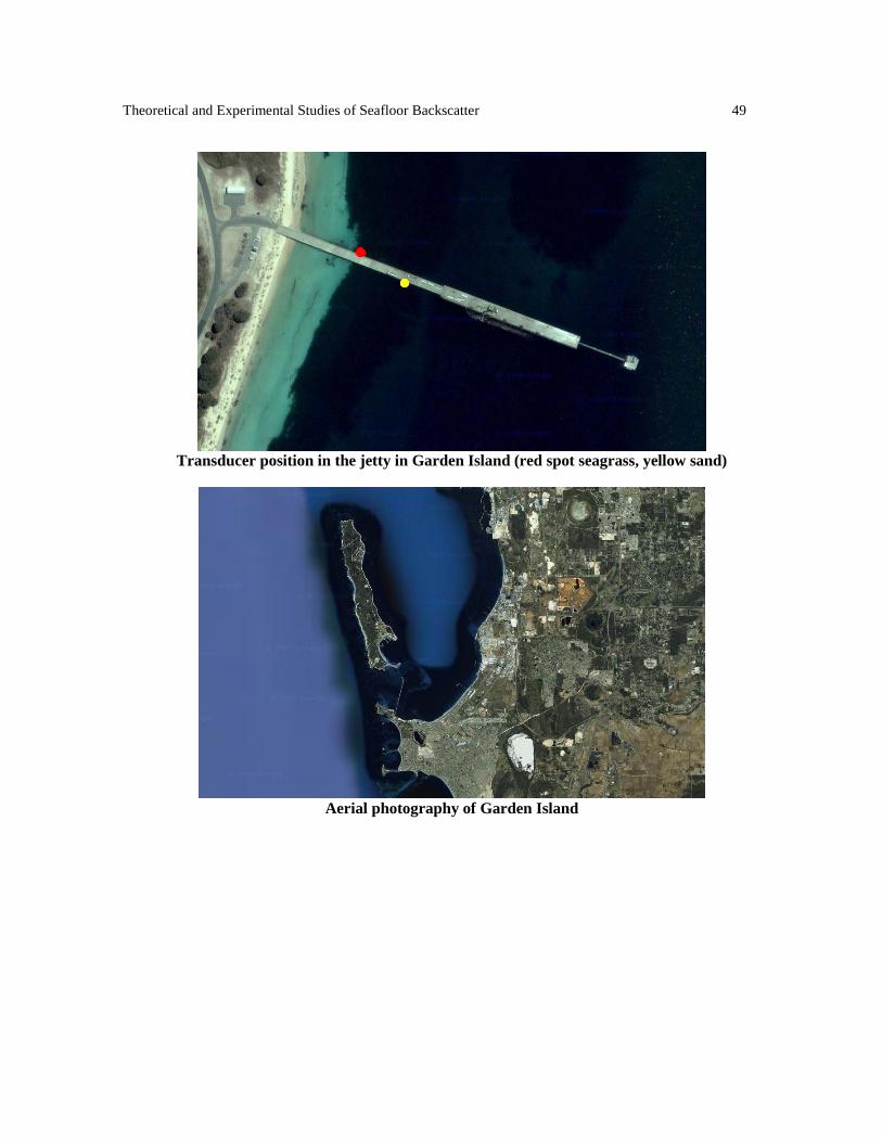
Theoretical and Experimental Studies of Seafloor Backscatter 49
Transducer position in the jetty in Garden Island (red spot seagrass, yellow sand)
Aerial photography of Garden Island