Theoretical analysis of spectrally encoded...

Theoretical analysis of spectrally encoded

endoscopy

Michal Merman, Avraham Abramov, and Dvir Yelin*

Department of Biomedical Engineering, Technion – Israel Institute of Technology, 32000 Haifa, Israel

*[email protected]

Abstract: Using a single optical fiber and miniature distal optics, spectrally-

encoded endoscopy (SEE) has been demonstrated as a promising, three-

dimensional endoscopic imaging method with a large number of resolvable

points and high frame rates. We present a detailed theoretical study of the

SEE prototype system and probe. Several key imaging parameters of SEE

are thoroughly derived and formulated, including the three-dimensional

point-spread function and field of view, as well as the system‟s optical

aberrations and fundamental limits. We find that the point-spread function

of the SEE system maintains a unique relation between its transverse and

axial shapes, discuss the asymmetry of the volumetric field of view,

determine that the number of lateral resolvable points is nearly twice than

what was previously accepted, and derive an expression for the upper limit

for the total number of resolvable points in the cross-sectional image plane.

© 2009 Optical Society of America

OCIS Codes: (110.2350) Fiber optics imaging; (170.2150) Endoscopic imaging; (110.4850)

Optical transfer functions; (110.2990) Image formation theory.

References and Links

1. C. M. Brown, P. G. Reinhall, S. Karasawa, and E. J. Seibel, “Optomechanical design and fabrication of resonant microscanners for a scanning fiber endoscope,” Opt. Eng. 45, 043001-043010 (2006).

2. D. L. Dickensheets, and G. S. Kino, “Silicon-micromachined scanning confocal optical microscope,” J.

Microelectromech. Syst. 7, 38–47 (1998). 3. A. L. Polglase, W. J. McLaren, S. A. Skinner, R. Kiesslich, M. F. Neurath, and P. M. Delaney, “A fluorescence

confocal endomicroscope for in vivo microscopy of the upper- and the lower-GI tract,” in Digestive Disease

Week/105th Annual Meeting of the American-Gastroenterological-Association (New Orleans, LA, 2004), pp. 686–695.

4. Y. C. Wu, Y. X. Leng, J. F. Xi, and X. D. Li, “Scanning all-fiber-optic endomicroscopy system for 3D nonlinear

optical imaging of biological tissues,” Opt. Express 17(10), 7907–7915 (2009). 5. G. J. Tearney, M. Shishkov, and B. E. Bouma, “Spectrally encoded miniature endoscopy,” Opt. Lett. 27(6), 412–

414 (2002).

6. D. Yelin, I. Rizvi, W. M. White, J. T. Motz, T. Hasan, B. E. Bouma, and G. J. Tearney, “Three-dimensional miniature endoscopy,” Nature 443(7113), 765 (2006).

7. D. Yelin, S. H. Yun, B. E. Bouma, and G. J. Tearney, “Three-dimensional imaging using spectral encoding

heterodyne interferometry,” Opt. Lett. 30(14), 1794–1796 (2005). 8. L. Froehly, S. N. Martin, T. Lasser, C. Depeursinge, and F. Lang, “Multiplexed 3D imaging using wavelength

encoded spectral interferometry: a proof of principle,” Opt. Commun. 222, 127–136 (2003).

9. D. Yelin, W. M. White, J. T. Motz, S. H. Yun, B. E. Bouma, and G. J. Tearney, “Spectral-domain spectrally-encoded endoscopy,” Opt. Express 15(5), 2432–2444 (2007).

10. M. A. Choma, M. V. Sarunic, C. H. Yang, and J. A. Izatt, “Sensitivity advantage of swept source and Fourier

domain optical coherence tomography,” Opt. Express 11(18), 2183–2189 (2003). 11. J. F. de Boer, B. Cense, B. H. Park, M. C. Pierce, G. J. Tearney, and B. E. Bouma, “Improved signal-to-noise

ratio in spectral-domain compared with time-domain optical coherence tomography,” Opt. Lett. 28(21), 2067–

2069 (2003). 12. R. Leitgeb, C. Hitzenberger, and A. Fercher, “Performance of fourier domain vs. time domain optical coherence

tomography,” Opt. Express 11(8), 889–894 (2003).

13. D. Yelin, B. E. Bouma, N. Iftimia, and G. J. Tearney, “Three-dimensional spectrally encoded imaging,” Opt. Lett. 28(23), 2321–2323 (2003).

14. D. Yelin, B. E. Bouma, and G. J. Tearney, “Volumetric sub-surface imaging using spectrally encoded

endoscopy,” Opt. Express 16(3), 1748–1757 (2008).

#115630 - $15.00 USD Received 17 Aug 2009; revised 28 Oct 2009; accepted 29 Oct 2009; published 17 Dec 2009

(C) 2009 OSA 21 December 2009 / Vol. 17, No. 26 / OPTICS EXPRESS 24045

15. D. Yelin, B. E. Bouma, J. J. Rosowsky, and G. J. Tearney, “Doppler imaging using spectrally-encoded

endoscopy,” Opt. Express 16(19), 14836–14844 (2008). 16. B. E. Bouma, and G. J. Tearney, eds., Handbook of Optical Coherence Tomography (Marcel Dekker, New York,

2002).

17. M. Wojtkowski, A. Kowalczyk, R. Leitgeb, and A. F. Fercher, “Full range complex spectral optical coherence tomography technique in eye imaging,” Opt. Lett. 27(16), 1415–1417 (2002).

18. K. B. Sung, C. N. Liang, M. Descour, T. Collier, M. Follen, and R. Richards-Kortum, “Fiber-optic confocal

reflectance microscope with miniature objective for in vivo imaging of human tissues,” IEEE Trans. Biomed. Eng. 49(10), 1168–1172 (2002).

19. C. Boudoux, S. Yun, W. Oh, W. White, N. Iftimia, M. Shishkov, B. Bouma, and G. Tearney, “Rapid wavelength-

swept spectrally encoded confocal microscopy,” Opt. Express 13(20), 8214–8221 (2005). 20. D. Yelin, C. Boudoux, B. E. Bouma, and G. J. Tearney, “Large area confocal microscopy,” Opt. Lett. 32(9),

1102–1104 (2007).

21. D. Yelin, B. E. Bouma, S. H. Yun, and G. J. Tearney, “Double-clad fiber for endoscopy,” Opt. Lett. 29(20),

2408–2410 (2004).

1. Introduction

Endoscopes are widely used in modern medical practice, making clinical procedures less

invasive and saving time and cost, while providing physicians with valuable information from

within the body. While current state-of-the-art clinical video endoscopes transmit excellent

image quality, their overall size is capped by the dimensions of their sensors and electronics.

Smaller and more flexible endoscopes have recently become available for clinical practice

using optical fiber bundles, where each individual fiber is used to transmit one pixel in an

image. Maintaining acceptable image quality with small diameter fiber bundles is challenging,

however; each optical fiber has a finite size, and therefore only a limited number of fibers can

be packed into an endoscope with a given diameter. Several research groups have attempted to

rapidly scan light from an optical fiber to obtain an image [1–4]. While high quality images

have been obtained using this technique, the size of the scanning mechanisms make rapid

distal scanning difficult to implement in the smallest endoscopic probes.

Recently, a single-fiber imaging technique termed spectrally encoded endoscopy (SEE)

was introduced [5], which replaced rapid scanning by spatial spectral encoding. SEE uses a

diffraction grating and a miniature lens to generate a spectrally resolved line on the sample,

which can be slowly scanned in one dimension to obtain a two-dimensional image with a large

number of resolvable points. Reducing the need for rapid scanning within the endoscopic

probe allows significant reduction in probe size, essentially trading the bulk and complexity of

a rapid scanning mechanism with a more sophisticated optical design, leaving the total probe

diameter limited only by the diameter of its optics [6].

Several methods for obtaining three-dimensional imaging in SEE have been proposed,

using time [7] and spectral [8,9] domain interferometric techniques. Compared to time-domain

interferometry, spectral domain interferometry offers orders-of-magnitude improvement in

signal-to-noise ratio (SNR) in optical coherence tomography (OCT), allowing improved

imaging quality and speed [10–12]. Spectral-domain SEE has been shown promising for

three-dimensional imaging [8,9,13], sub-surface volumetric imaging [14], and Doppler

imaging [15].

A fundamental optical analysis of multiplexed three-dimensional imaging using

wavelength encoded spectral interferometry was first presented by Froehly et al. [8], and

various approximated expressions are often being used to estimate the imaging parameters of

spectrally encoded endoscopy [5,9]. In this paper, a detailed theoretical analysis of the SEE

system [6] is presented in which we account for the effects of the probe‟s limited circular

aperture, its optical aberrations, and the finite resolution of the spectrometer. We first outline

and formulate the interferometric SEE working principles, derive the system‟s point-spread

function (PSF) and its three-dimensional field of view using diffraction theory, and study the

effect of the various optical aberrations that are present in the system.



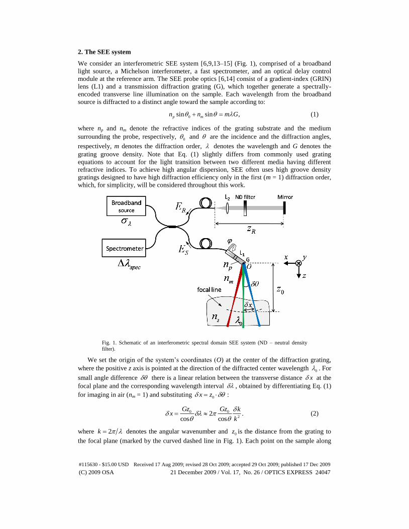
2. The SEE system

We consider an interferometric SEE system [6,9,13–15] (Fig. 1), comprised of a broadband

light source, a Michelson interferometer, a fast spectrometer, and an optical delay control

module at the reference arm. The SEE probe optics [6,14] consist of a gradient-index (GRIN)

lens (L1) and a transmission diffraction grating (G), which together generate a spectrally-

encoded transverse line illumination on the sample. Each wavelength from the broadband

source is diffracted to a distinct angle toward the sample according to:

0sin sin ,p mn n m G (1)

where np and nm denote the refractive indices of the grating substrate and the medium

surrounding the probe, respectively, 0 and are the incidence and the diffraction angles,

respectively, m denotes the diffraction order, denotes the wavelength and G denotes the

grating groove density. Note that Eq. (1) slightly differs from commonly used grating

equations to account for the light transition between two different media having different

refractive indices. To achieve high angular dispersion, SEE often uses high groove density

gratings designed to have high diffraction efficiency only in the first (m = 1) diffraction order,

which, for simplicity, will be considered throughout this work.

Fig. 1. Schematic of an interferometric spectral domain SEE system (ND – neutral density

filter).

We set the origin of the system‟s coordinates (O) at the center of the diffraction grating,

where the positive z axis is pointed at the direction of the diffracted center wavelength 0 . For

small angle difference there is a linear relation between the transverse distance x at the

focal plane and the corresponding wavelength interval , obtained by differentiating Eq. (1)

for imaging in air (nm = 1) and substituting 0x z :

0 0

22 .

cos cos

Gz Gz kx

k

(2)

where 2k denotes the angular wavenumber and 0z is the distance from the grating to

the focal plane (marked by the curved dashed line in Fig. 1). Each point on the sample along



the spectral line is illuminated by light with spectral bandwidth k . In a high quality imaging

system with more than hundred resolvable elements per line, we can assume that the spectral

bandwidth illuminating each transverse sample location k is significantly smaller than the

total source bandwidth k , i.e.

kk .

Scanning the spectrally encoded line in the perpendicular transverse coordinate (y axis) is

accomplished by scanning the angle (see Fig. 1), rotating the SEE probe around its optical

axis. In recent works a galvanometric scanner (Cambridge Technology, Inc., not shown in Fig.

1) was used for probe rotation, which was limited to a maximum mechanical scanning angle

of 20° [6,9]. The third axial dimension is obtained by allowing the light reflected from the

sample back into the probe to interfere with light from the reference mirror on a fast linear

CCD camera within a high resolution spectrometer.

While several different configurations of SEE could be considered for different

applications, we choose to base our analysis on the probe design that was first published in

Ref [6]. and was later used in Refs [9,14,15]. While other probe designs may have somewhat

different optical parameters and feature sets, they would share many of the imaging principles

and limitations of the SEE technique which are derived below.

3. SEE prototype analysis

3.1 Probe structure and components

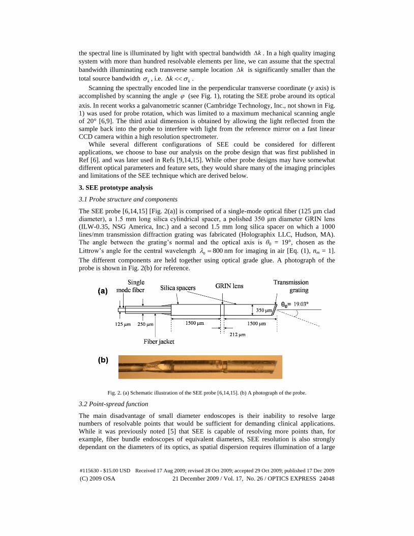
The SEE probe [6,14,15] [Fig. 2(a)] is comprised of a single-mode optical fiber (125 µm clad

diameter), a 1.5 mm long silica cylindrical spacer, a polished 350 μm diameter GRIN lens

(ILW-0.35, NSG America, Inc.) and a second 1.5 mm long silica spacer on which a 1000

lines/mm transmission diffraction grating was fabricated (Holographix LLC, Hudson, MA).

The angle between the grating‟s normal and the optical axis is θ0 = 19°, chosen as the

Littrow‟s angle for the central wavelength 0 800 nm for imaging in air [Eq. (1), nm = 1].

The different components are held together using optical grade glue. A photograph of the

probe is shown in Fig. 2(b) for reference.

Fig. 2. (a) Schematic illustration of the SEE probe [6,14,15]. (b) A photograph of the probe.

3.2 Point-spread function

The main disadvantage of small diameter endoscopes is their inability to resolve large

numbers of resolvable points that would be sufficient for demanding clinical applications.

While it was previously noted [5] that SEE is capable of resolving more points than, for

example, fiber bundle endoscopes of equivalent diameters, SEE resolution is also strongly

dependant on the diameters of its optics, as spatial dispersion requires illumination of a large



number of grating lines. In order to derive the theoretical PSF of the SEE probe at the center

of the field of view (FOV), we will assume that the beam emitted from the optical fiber over-

fills the aperture of the GRIN lens, maximizing its effective numerical aperture, as well as the

illuminated area of the grating. We assume that the lens is illuminated on its optical axis by a

perfect spherical wave, and neglect optical aberrations, which will be addressed in detail in

Sections 3.5-3.6.

Consider first a monochromatic point source P located at the fiber core, from which light

propagates via a lens of diameter D and is deflected by a grating, as schematically depicted in

Fig. 3. According to Fresnel diffraction theory, the field distribution EM at the focal plane z0 of

the SEE probe for monochromatic illumination of angular wavenumber km, is given by:

2 2

0

2 2

1 022

0 02 2

0

2

, , , ,

2

mm

km mi x x y

z

M m m m

m m

J k D x x y z

E k x y z E k Ck e

k D x x y z

(3)

where C denotes a scaling constant containing uniform spectral attenuations in the optical

system, E0 denotes the source field amplitude, and xm denotes the location of the first

diffraction order for km (Fig. 3, red solid lines). For simplicity, we will consider the field at

0y , and omit the y coordinate from the following equations.

For deriving the PSF, we consider a sample with a single point reflector of reflectivity r0

located at xs: 0S sr x r x x , where denotes the Dirac delta function. When the

illumination field contains a continuum of wavelengths with a total bandwidth k , the total

amplitude of the illumination field at xs is obtained by integrating over all angular

wavenumbers: 0 0 0, , ,k

S s m M m sE x z r dk E k x z

.

Fig. 3. Schematic illustration of the illumination and signal collection optical paths in SEE.

The back-reflected light propagation from the sample to the probe is governed by the same

diffraction principles that are valid for the illumination, and the field collected by the fiber

core from a point reflector at xs for any wavenumber k is given by:

2

01 022

0 0

0

2, , , , ,

2

s k

ki x x

s kz

C s S s

s k

J kD x x zE k x z CE k x z k e

kD x x z

(4)

where 0, ,C sE k x z denotes the collected monochromatic field and xk denotes the location of

the first diffraction order, corresponding to the angular wavenumber k (Fig. 3, blue dashed

lines). The field 0, ,S sE k x z can be calculated using a “spectral overlap” function ,mf k k ,

which expresses the overlap between an illuminating channel km and a collection channel k:

0 0 0, , , , , .k

S s m M m s mE k x z r dk E k x z f k k

(5)



Using the single-mode fiber core as an effective pinhole, the SEE probe is essentially a

confocal optical arrangement in which both the illumination and the collection optical paths

overlap in space, i.e. ,m mf k k k k . Substituting ,mf k k , Eq. (2) and Eq. (5) into

Eq. (4), we obtain, after a change of variables, the spectral distribution of the field returning

from the sample to the fiber core:

2

0

20 0

22

1 0cos2 4

0 0 0

0

cos, , ,

cos

sGz k kki

sz k

C s

s

J DG k k kE k k z E k r C k e

DG k k k

(6)

where ks is the wavenumber whose first diffraction order is located at the scatterer location xs,

and where we have assumed that 0cos cos for the spectral region around the central

wavelength at the center FOV.

The (field) PSF of SEE is thus given by:

0 0 0 0, , , , ,s C sh k k z E k k z E k r (7)

and its full width at half maximum (FWHM) is given by: 01.029 cosk k DG , and in

terms of wavelength:

0cos1.029 .

DG

(8)

The intensity PSF 2

h k , has a FWHM given by 00.738 cos /kS k DG , and in terms

of spatial coordinates, using Eq. (2):

00.738 ,X

zS

D

(9)

where the numerical coefficient was derived numerically from the intensity PSF. Due to the

circular symmetry near the optical axis, a similar expression can be derived from Eq. (3) for

the FWHM along the y axis: Y XS S . Substituting the system‟s and probe‟s parameters from

Ref [6]. into Eq. (9) yields 0 10mm 16.87XS z µm at the central wavelength,

representing the aberration-free, Fourier-limited system performance at the center FOV.

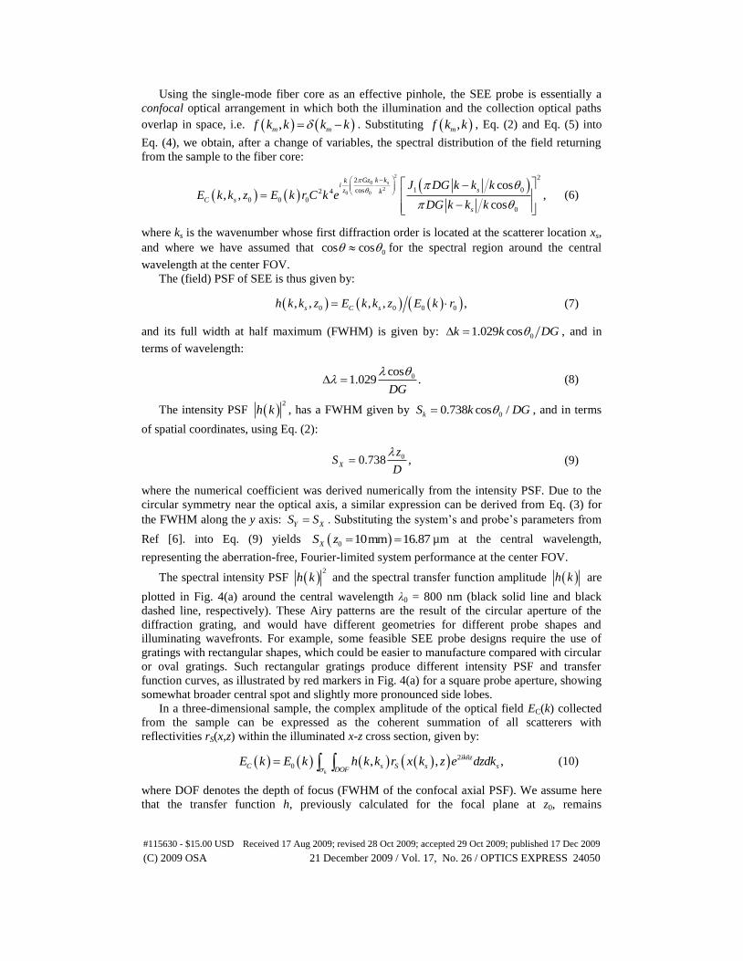
The spectral intensity PSF 2

h k and the spectral transfer function amplitude h k are

plotted in Fig. 4(a) around the central wavelength λ0 = 800 nm (black solid line and black

dashed line, respectively). These Airy patterns are the result of the circular aperture of the

diffraction grating, and would have different geometries for different probe shapes and

illuminating wavefronts. For example, some feasible SEE probe designs require the use of

gratings with rectangular shapes, which could be easier to manufacture compared with circular

or oval gratings. Such rectangular gratings produce different intensity PSF and transfer

function curves, as illustrated by red markers in Fig. 4(a) for a square probe aperture, showing

somewhat broader central spot and slightly more pronounced side lobes.

In a three-dimensional sample, the complex amplitude of the optical field EC(k) collected

from the sample can be expressed as the coherent summation of all scatterers with

reflectivities rS(x,z) within the illuminated x-z cross section, given by:

2

0 , , ,k

iknz

C s S s sDOF

E k E k h k k r x k z e dzdk

(10)

where DOF denotes the depth of focus (FWHM of the confocal axial PSF). We assume here

that the transfer function h, previously calculated for the focal plane at z0, remains



approximately unchanged within DOF. The distance z0 is given by 0 m sz z z , where zm and

zs denote the propagation distances in the medium and in the sample, respectively. For

simplicity, we assumed that the probe optics have a total length that is much smaller than its

working distance z0, thus we can neglect phase accumulation inside the probe. This

assumption is justified by realizing that the 1.5 mm separation between the lens and the

grating (Fig. 2) is a result of the specific manufacturing process, and could be made much

smaller in future versions of the probe. The weighted refractive index is given by

0s m m s sn z n z n z z , where nm and ns denote the refractive indices of the medium and

the sample, respectively.

Fig. 4. (a) Lateral intensity PSF (black solid line) and the spectral impulse response |h(λ)| (black

dashed line) of SEE probe with a uniformly illuminated circular aperture and a working

distance of 10 mm. A rectangular aperture produces a slightly different lateral spectral transfer function (hollow red squares) and PSF (filled red squares). (b) Interferometric axial PSF of

confocal SEE (black solid) compared to the PSF of a confocal system with rectangular aperture

(red dashed). The top axis axial coordinates assume ns = 1.

In the reference arm, the complex amplitude of the optical field reflected from a mirror

with reflectivity rR is given by:

2

0 ,Rikz

R RE k E k r e (11)

where zR denotes the distance between the fiber exit and the reference mirror (Fig. 1).

Constant attenuations in both arms were neglected for clarity. In order to calculate the

interferometric axial PSF, we consider the spectral interference between the returning

reference and sample signals, captured by the spectrometer line camera, which can be

expressed as the coherent summation of the fields from the reference (Eq. (11)) and sample

(Eq. (10)) arms:

222 2 2

0

2

, ,

2 Re , , .

k

R

k

iknz

R S R s S s sDOF

ik nz z

R s S s sDOF

I k E E E k r h k k r x k z e dzdk

r h k k r x k z e dzdk

(12)

The first term on the right hand side of Eq. (12) represents the intensity reflected from the

reference arm, which could be experimentally measured by blocking the light returning from



the sample arm. The second term represents the self-interference of light from different axial

scatterers within the sample, and the third term represents the cross-interference between the

sample and reference fields, containing the cross-sectional distribution of the reflections

within the sample.

At this point it is worth noting that by substituting G = 0 in Eq. (7) (meaning essentially

no diffraction grating in the probe) we obtain from Eq. (12) an expression for the spectral

interference in spectral domain OCT (SD-OCT) [16] (neglecting constant attenuation factors):

22 2 2

0 2 cos 2 ,iknz

OCT R S R S RDOF DOF

I k E k r r z e dz r r z k nz z dz

(13)

where the sample reflectivity rS(z) is a function of the z coordinate only. OCT could be

therefore viewed as private case of SEE, in the limit where the number of transverse

resolvable points in SEE equals 1. A comparison between SD-OCT and SD-SEE has been

previously described in Ref [14].

We may now neglect the phase term of the spectral transfer function , sh k k in Eq. (7) by

noting that it changes very little (by approximately 0.2 radians) over its own spectral width

k . The impulse response , sh k k [Eq. (7)] then becomes a real function, and the cross-

interference term in Eq. (12) is given by:

2

02 , , cos ,k

CI R s S s sDOF

I k r E h k k r x k z k dzdk

(14)

where 2 Rnz z denotes the modulation frequency of the interference patterns on the

spectrometer, and we have assumed that the source spectrum varies slowly over the entire

width ( k ) of h k , hence 0 0E k E . Equation (14) implies that the axial resolution is

related to the spectral width of h k , which is related to the lateral PSF through the spatial

coordinate encoding [Eq. (2)].

Using a single scatterer representation in the cross sectional x-z plane:

0,S Sr x z r x z z and substituting it into Eq. (14), we obtain:

2

0 0 0 02 0, cos ,CI R SI k r r z E h k k k (15)

where 0 02 Rnz z . The optical path difference between light reflected from a single

point at the sample, and from the reference mirror can now be calculated using a Fourier

transformation of Eq. (15) over the entire spectral bandwidth k :

0 0 0 0 ,CII I FT I k I H (16)

where 2

0 0 02 0,R SI E r r z , and H FT h k . The problem of depth ambiguity,

manifested through the emergence of two axially symmetric images for each scatterer, is a

result of the real-part only spectral measurement of the spectrometer, and could be solved by

acquiring a second spectral measurement with the reference mirror relocated to induce a 2

phase shift in the reference plane, and combining two spectral measurements to retrieve the

complex spectral amplitude [9,14]. This technique would allow utilizing the full resolution

power of the spectrometer and doubling the imaging depth range compared to a single spectral

acquisition. In addition, similar techniques were shown useful in SD-OCT [17] for effectively

removing the reference background and the effect of the sample self interference.



A plot of I is shown in Fig. 4(b) for circular (black solid line) and rectangular (red

dashed line) probe apertures. The triangular profile of the axial PSF in Fig. 4(b) is an

interesting and unique feature of SEE, resulting from Fourier-transforming a sinc-squared

function, which may suggests a possible resolution advantage over circular apertures in high

SNR imaging conditions.

Solving Eq. (16) numerically, we obtain an expression for the FWHM of the axial PSF:

2

0 0

0

0.45 0.463 .cos

Z

S S

DGS

n n

(17)

We note that by replacing with the total source bandwidth , Eq. (17) can be used to

approximate the axial resolution of OCT. Since SEE uses the spectrum primarily to encode

space, its axial resolution is lower than that of OCT [14] by a factor approximately equal to

the number of spectrally resolved spectral points . Substituting the system‟s and

probe‟s parameters from Ref. [6]. into Eq. (17) yields 135ZS μm, representing the

aberration-free, Fourier-limited axial resolution at the central FOV.

3.3 Field of view

In order to obtain approximate analytical expressions for the field of view of SEE, we first

simplify Eq. (1) by using the small angle approximation, sin , and by assuming that is

linear with across the entire source spectrum . Equation (2) would then hold for the

entire lateral image area, i.e.:

0

0

.cos

GzX

(18)

In the y axis, the field of view depends on the scanning angle of the galvanometric scanner

(see Ref [9].). Applying a full, continuous 360° rotation of the probe using an optical rotary

junction would allow maximizing the lateral field of view and could reduce mechanical

vibrations. The geometry of the three dimensional field of view in this configuration is

discussed in Section 3.6. In some clinical applications, continuous saw-tooth scanning of the

rotation angle is desired in order to produce high frame rates at nearly rectangular fields of

view. For small rotation angles, the lateral FOV in the y axis is given by:

02 tan( ),Y z (19)

where 2 denotes the amplitude of the probe rotation angle (Fig. 1).

The axial imaging range of the SEE probe is limited by the spectrometer‟s ability to

resolve high spectral modulation frequencies (denoted by in Section 3.2). The total imaging

range in the z axis is then derived from the Nyquist sampling limit and is given by:

2

.spec

Z

(20)

Note that the expression in Eq. (20) is independent on spectral encoding, and is valid for

SD-OCT as well. The axial imaging range could be extended beyond this limit by stepping the

reference mirror position between consecutive spectral acquisitions [9]. This approach would

require sophisticated data acquisition and processing, and would eventually be limited by the

total depth of focus of the probe‟s optics.



3.4 Resolvable points

The number of resolvable points is a critical parameter in small diameter endoscopes for

evaluating the amount of information within a single image. In the spectrally encoded x axis,

the number of resolvable points can be approximated by calculating the ratio between the field

of view and the spatial resolution:

0 0

1.355 .cos

X

X

GDXN

S

(21)

Similarly, for the y axis, the number of resolvable points is given by:

0

2 tan1.355 .Y

Y

DYN

S

(22)

Similar expressions to those of Eqs. (21) and (22) have been used for estimating the

number of resolvable points in previous works ([5,8,9]), the only difference being the

numerical constant 1.355, which is a consequence of the smaller confocal lateral PSF. Overall,

we find a total of 21.355 1.84 increase in the number of resolvable points in the lateral plane

compared to what was previously accepted for SEE.

The number of axial resolvable points in SEE is limited by the number of resolvable

spectral modulation frequencies ( ), which is equal to the number of resolvable elements

spec within each bandwidth fraction encoding each lateral resolvable element:

.Z specN (23)

For the parameters of the experimental system in Ref [6]. we obtain 188XN ,

209YN , and 22ZN . The theoretical number of resolvable points in the lateral x-y plane

is 1.5 times more than previously predicted [9,14].

Equation (21) and Eq. (23) are both derived from a single spectral acquisition. Using Eq.

(8), the product of these expressions represents the single-shot total number of cross sectional

(x-z plane) resolvable points:

1.39 .X Z

spec

N N

(24)

Interestingly, the total number of resolvable points in the x-z plane is independent of the

optical parameters of the probe, only on the source and spectrometer properties. Therefore,

Eq. (24) represents a fundamental upper limit of the spectral encoding technique, implying

that the spectral content of the SEE system eventually limits its imaging performance,

operating as an „information resource‟ for the system.

3.5 Optical aberrations

In the above analysis, Eqs. (9) and (17) express the transform-limited PSF width for the center

wavelength at Littrow angle, and therefore represent the upper limit for the resolution for the

SEE prototype system. Various optical aberrations are present in the current design of the SEE

probe, which affect image quality, resolution, and field of view. In the following analysis,

optical design software (ZEMAX Development Corporation, Washington, USA) was used to

analyze several key imaging parameters, including the lateral PSF and focal plane geometry.

A two-dimensional layout of the SEE probe and the light rays at three representative

wavelengths are shown in Fig. 5. A close-up view of the rays within the probe (Fig. 5, inset)

shows the diverging wave from the single-mode fiber over-fills the GRIN lens aperture, which

slowly focuses the beam at the focal plane. The curved focal line, marked by a black solid

line, connects axial points along the rays with the smallest diameter transverse spot. The



diffraction angle between the central wavelength (800 nm) and the probe‟s optical axis is 38°,

which equals twice the Littrow‟s angle. The rest of the spectrum is diffracted around the

central wavelength, generating a spectral line on the sample located approximately 10 mm

from the grating. The properties of the simulated GRIN lens are summarized in Fig. 5.

Fig. 5. Simulations of the light rays illuminating the sample through the SEE probe. A

magnified view of the probe‟s drawing is shown in the inset.

Due to the unique design of the probe optics, some optical aberrations are manifested in a

different way than in conventional imaging systems. The effect of coma aberrations due to

non-axial rays in the lens is practically nonexistent in the SEE probe since the broadband light

emitted from the single mode fiber propagates only in the probe‟s optical axis and illuminates

the lens axially. The spherical aberrations induced by the GRIN lens are also negligible due to

the non-spherical surfaces of the lens. Based on ZEMAX simulations we estimate that

spherical aberrations cause less than 0.5% broadening of the lateral PSF across the entire focal

plane (data not shown).

In order to quantify and isolate the effect of chromatic aberrations, we have computed the

focal shift and the spot size of the illumination rays for different wavelengths within the

source spectral range without the presence of the grating, and with the distal surface of the

probe perpendicular to the optical axis (not at Littrow‟s angle). The main effect of chromatic

aberrations in SEE is evident on the axial location of the focal line (Fig. 6), where each

wavelength is focused at different axial distance from the lens. We have calculated a focal

plane tilt of approximately 8.5° in the x-z plane as a result of chromatic aberrations only.

Fig. 6. Focal shift induced by chromatic aberrations for a working distance of 10 mm for the

center wavelength.

We have found that chromatic aberrations impose approximately 1% (0.1 μm) broadening

of the PSF. This negligible influence of chromatic aberrations on resolution results from the



relatively small bandwidth fraction Δλ (Eq. (8)) illuminating each sample location, and may

help in reducing the cost and complexity of future miniature lenses [18].

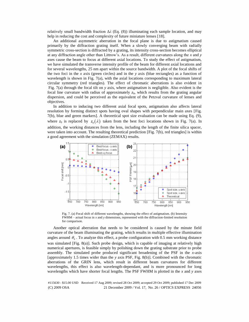
An additional asymmetric aberration in the focal plane is due to astigmatism caused

primarily by the diffraction grating itself. When a slowly converging beam with radially

symmetric cross-section is diffracted by a grating, its intensity cross-section becomes elliptical

at any diffraction angle other than Littrow‟s. As a result, different curvatures along the x and y

axes cause the beam to focus at different axial locations. To study the effect of astigmatism,

we have simulated the transverse intensity profile of the beam for different axial locations and

for several wavelengths, 25 nm apart within the source bandwidth. A plot of the focal shifts of

the two foci in the x axis (green circles) and in the y axis (blue rectangles) as a function of

wavelength is shown in Fig. 7(a), with the axial locations corresponding to maximum lateral

circular symmetry (red triangles). The effect of chromatic aberrations is also evident in

Fig. 7(a) through the focal tilt on y axis, where astigmatism is negligible. Also evident is the

focal line curvature with radius of approximately z0, which results from the grating angular

dispersion, and could be perceived as the equivalent of the Petzval curvature of lenses and

objectives.

In addition to inducing two different axial focal spots, astigmatism also affects lateral

resolution by forming distinct spots having oval shapes with perpendicular main axes [Fig.

7(b), blue and green markers]. A theoretical spot size evaluation can be made using Eq. (9),

where z0 is replaced by 0z taken from the best foci locations shown in Fig. 7(a). In

addition, the working distances from the lens, including the length of the finite silica spacer,

were taken into account. The resulting theoretical prediction [Fig. 7(b), red triangles] is within

a good agreement with the simulation (ZEMAX) results.

Fig. 7. (a) Focal shift of different wavelengths, showing the effect of astigmatism. (b) Intensity FWHM – actual focus in x and y dimensions, represented with the diffraction-limited resolution

for comparison.

Another optical aberration that needs to be considered is caused by the minute field

curvature of the beam illuminating the grating, which results in multiple effective illumination

angles around 0 . To analyze this effect, a probe configuration with 0.5 mm working distance

was simulated [Fig. 8(a)]. Such probe design, which is capable of imaging at relatively high

numerical apertures, is feasible simply by polishing down the grating substrate prior to probe

assembly. The simulated probe produced significant broadening of the PSF in the x-axis

[approximately 1.5 times wider than the y axis PSF, Fig. 8(b)]. Combined with the chromatic

aberrations of the GRIN lens, which result in different beam curvatures for different

wavelengths, this effect is also wavelength-dependant, and is more pronounced for long

wavelengths which have shorter focal lengths. The PSF FWHM is plotted in the x and y axes



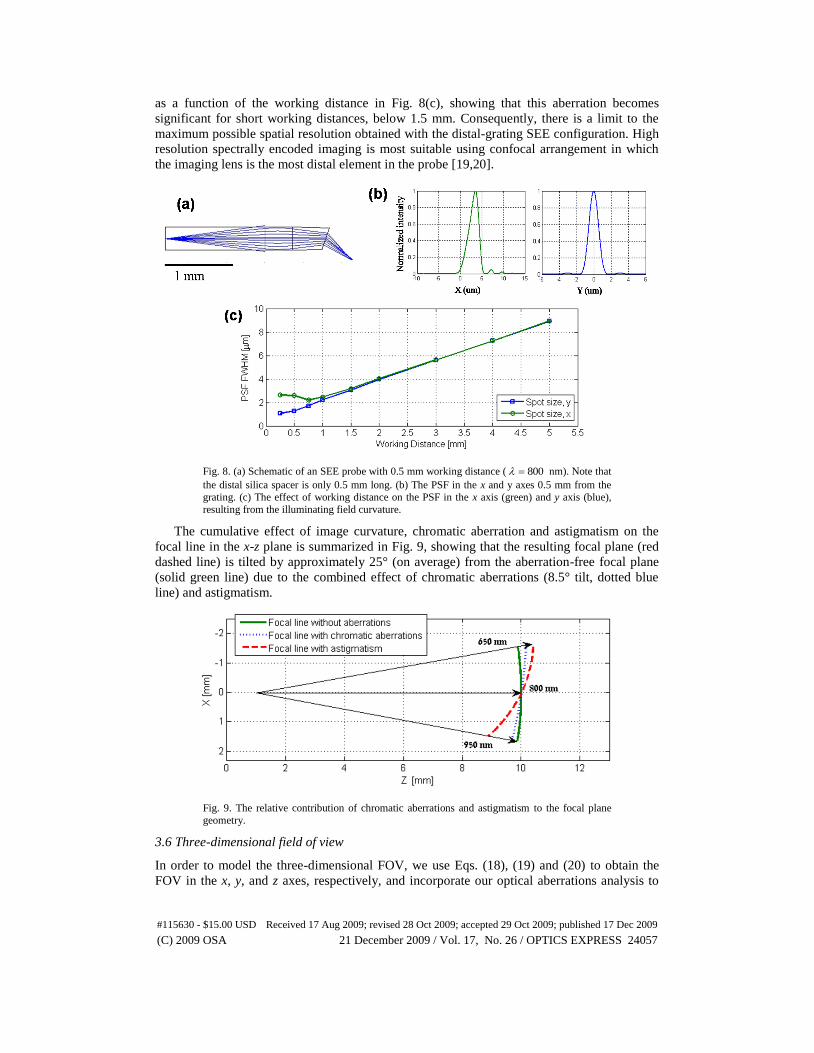
as a function of the working distance in Fig. 8(c), showing that this aberration becomes

significant for short working distances, below 1.5 mm. Consequently, there is a limit to the

maximum possible spatial resolution obtained with the distal-grating SEE configuration. High

resolution spectrally encoded imaging is most suitable using confocal arrangement in which

the imaging lens is the most distal element in the probe [19,20].

Fig. 8. (a) Schematic of an SEE probe with 0.5 mm working distance ( 800 nm). Note that

the distal silica spacer is only 0.5 mm long. (b) The PSF in the x and y axes 0.5 mm from the

grating. (c) The effect of working distance on the PSF in the x axis (green) and y axis (blue),

resulting from the illuminating field curvature.

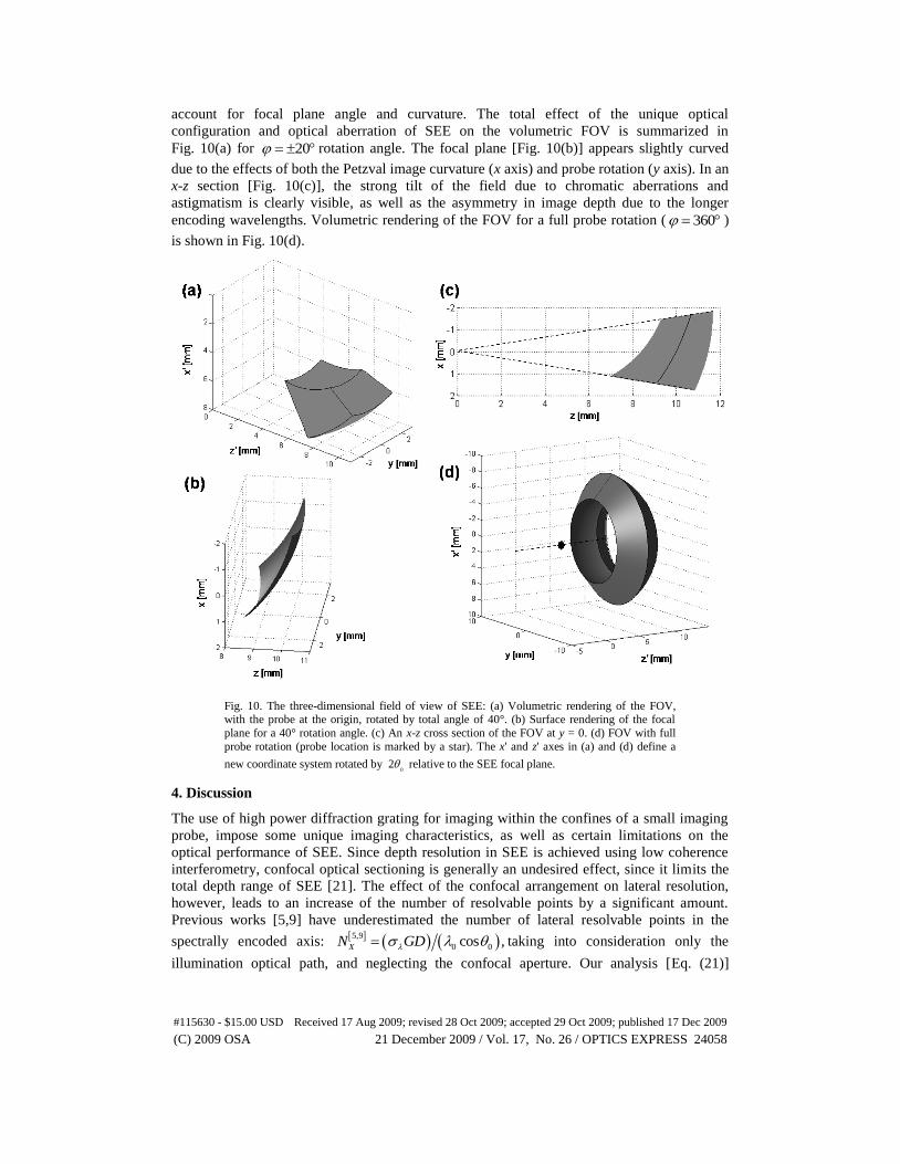
The cumulative effect of image curvature, chromatic aberration and astigmatism on the

focal line in the x-z plane is summarized in Fig. 9, showing that the resulting focal plane (red

dashed line) is tilted by approximately 25° (on average) from the aberration-free focal plane

(solid green line) due to the combined effect of chromatic aberrations (8.5° tilt, dotted blue

line) and astigmatism.

Fig. 9. The relative contribution of chromatic aberrations and astigmatism to the focal plane

geometry.

3.6 Three-dimensional field of view

In order to model the three-dimensional FOV, we use Eqs. (18), (19) and (20) to obtain the

FOV in the x, y, and z axes, respectively, and incorporate our optical aberrations analysis to



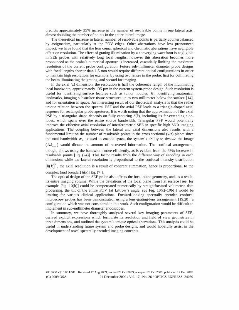
account for focal plane angle and curvature. The total effect of the unique optical

configuration and optical aberration of SEE on the volumetric FOV is summarized in

Fig. 10(a) for 20 rotation angle. The focal plane [Fig. 10(b)] appears slightly curved

due to the effects of both the Petzval image curvature (x axis) and probe rotation (y axis). In an

x-z section [Fig. 10(c)], the strong tilt of the field due to chromatic aberrations and

astigmatism is clearly visible, as well as the asymmetry in image depth due to the longer

encoding wavelengths. Volumetric rendering of the FOV for a full probe rotation ( 360 )

is shown in Fig. 10(d).

Fig. 10. The three-dimensional field of view of SEE: (a) Volumetric rendering of the FOV, with the probe at the origin, rotated by total angle of 40°. (b) Surface rendering of the focal

plane for a 40° rotation angle. (c) An x-z cross section of the FOV at y = 0. (d) FOV with full

probe rotation (probe location is marked by a star). The x' and z' axes in (a) and (d) define a

new coordinate system rotated by 0

2 relative to the SEE focal plane.

4. Discussion

The use of high power diffraction grating for imaging within the confines of a small imaging

probe, impose some unique imaging characteristics, as well as certain limitations on the

optical performance of SEE. Since depth resolution in SEE is achieved using low coherence

interferometry, confocal optical sectioning is generally an undesired effect, since it limits the

total depth range of SEE [21]. The effect of the confocal arrangement on lateral resolution,

however, leads to an increase of the number of resolvable points by a significant amount.

Previous works [5,9] have underestimated the number of lateral resolvable points in the

spectrally encoded axis: 5,9

0 0cos ,XN GD taking into consideration only the

illumination optical path, and neglecting the confocal aperture. Our analysis [Eq. (21)]



predicts approximately 35% increase in the number of resolvable points in one lateral axis,

almost doubling the number of points in the entire lateral image.

The theoretical increase in lateral number of resolvable points is partially counterbalanced

by astigmatism, particularly at the FOV edges. Other aberrations have less pronounced

impact: we have found that the lens coma, spherical and chromatic aberrations have negligible

effect on resolution. The effect of grating illumination by a converging wavefront is negligible

in SEE probes with relatively long focal lengths; however this aberration becomes more

pronounced as the probe‟s numerical aperture is increased, essentially limiting the maximum

resolution of the current probe configuration. Future sub-millimeter diameter probe designs

with focal lengths shorter than 1.5 mm would require different optical configurations in order

to maintain high resolution, for example, by using two lenses in the probe, first for collimating

the beam illuminating the grating, and second for imaging.

In the axial (z) dimension, the resolution is half the coherence length of the illuminating

local bandwidth, approximately 135 µm in the current system-probe design. Such resolution is

useful for identifying surface features such as tumor nodules [6], identifying anatomical

landmarks, imaging subsurface tissue structures up to two millimeter below the surface [14],

and for orientation in space. An interesting result of our theoretical analysis is that the rather

unique relation between the spectral PSF and the axial PSF leads to a triangle-shaped axial

response for rectangular probe apertures. It is worth noting that the approximation of the axial

PSF by a triangular shape depends on fully capturing h(k), including its far-extending side-

lobes, which spans over the entire source bandwidth. Triangular PSF would potentially

improve the effective axial resolution of interferometric SEE in specific high SNR imaging

applications. The coupling between the lateral and axial dimensions also results with a

fundamental limit on the number of resolvable points in the cross sectional (x-z) plane: since

the total bandwidth is used to encode space, the system‟s ability to decode the image

( spec ) would dictate the amount of recovered information. The confocal arrangement,

though, allows using the bandwidth more efficiently, as is evident from the 39% increase in

resolvable points [Eq. (24)]. This factor results from the different way of encoding in each

dimension: while the lateral resolution is proportional to the confocal intensity distribution

2

h k , the axial resolution is a result of coherent summation, hence is proportional to the

complex (and broader) h(k) [Eq. (7)].

The optical design of the SEE probe also affects the focal plane geometry, and, as a result,

its entire imaging volume. While the deviations of the focal plane from flat surface [see, for

example, Fig. 10(b)] could be compensated numerically by straightforward volumetric data

processing, the tilt of the entire FOV [at Littrow‟s angle, see Fig. 10(c)–10(d)] would be

limiting for various clinical applications. Forward-looking spectrally encoded confocal

microscopy probes has been demonstrated, using a lens-grating-lens arrangement [19,20], a

configuration which was not considered in this work. Such configuration would be difficult to

implement in sub-millimeter diameter endoscopes.

In summary, we have thoroughly analyzed several key imaging parameters of SEE,

derived explicit expressions which formulate its resolution and field of view geometries in

three dimensions, and outlined the system‟s unique optical aberrations. This analysis could be

useful in understanding future system and probe designs, and would hopefully assist in the

development of novel spectrally encoded imaging concepts.



Theoretical analysis of spectrally encoded...

Documents

Transcript of Theoretical analysis of spectrally encoded...