J Autom ReasoningDOI 10.1007/s10817-013-9299-0

Theorem of Three Circles in Coq

Julianna Zsido

Received: 7 June 2013 / Accepted: 4 December 2013© Springer Science+Business Media Dordrecht 2013

Abstract The theorem of three circles in real algebraic geometry guarantees the termina-tion and correctness of an algorithm of isolating real roots of a univariate polynomial. Themain idea of its proof is to consider polynomials whose roots belong to a certain area of thecomplex plane delimited by straight lines. After applying a transformation involving inver-sion this area is mapped to an area delimited by circles. We provide a formalisation of thisrather geometric proof in Ssreflect, an extension of the proof assistant Coq, that supports avariety of algebraic tools. They allow us to formalise the proof from an algebraic point ofview.

Keywords Formalisation · Coq · Three circles · Bernstein coefficients · Normalpolynomial · Real root isolation

1 Introduction

The theorem of three circles that is the subject of this paper is not to be confused withthe Hadamard three circle theorem in complex analysis. Our area of interest is algorithmicreal algebraic geometry, for which [1] is our main reference hereinafter. Before stating thetheorem of three circles, which is called as such in [1], chapter 10, we first introduce somenecessary vocabulary and notations.

Electronic supplementary material The online version of this article(doi:10.1007/s10817-013-9299-0) contains supplementary material, whichis available to authorized users.

J. Zsido (�)INRIA Sophia Antipolis, 2004 route des Lucioles, BP 93, 06902 Sophia Antipolis Cedex, Francee-mail: julianna.zsido@gmail.com

J. Zsido

Let us fix an open real interval (l, r) and consider the following three open discs of thecomplex plane, see Fig. 1:

– C0 the disc bound by the circle with diameter (l, r);– C1 the disc bound by the circumcircle of the equilateral triangle with base (l, r) and

whose vertices have non-negative imaginary parts;– C2 the disc symmetric to C1 with respect to the real axis.

Next we give some intuitive elements of the theory of so–called Bernstein polynomialsneeded for the theorem of three circles. Bernstein polynomials are associated to a certaininterval (a, b), and a degree n, see Fig. 2 for (a, b) = (0, 1), n = 3 and n = 4. They form abasis of �n, the vector space of polynomials of degree at most n. Bernstein polynomials canbe used to approximate continuous functions on (a, b). Moreover they provide the controlpoints for Bezier curves, which play an important role in image manipulation programs forexample.

The coefficients of a polynomial expressed in the Bernstein basis are its Bernstein co-efficients. In Fig. 2, we can see that the Bernstein polynomials have maxima in differentpoints. Given a polynomial in a Bernstein basis, intuitively speaking each Bernstein coeffi-cient describes the behaviour of the polynomial in an interval around the maximum of thecorresponding Bernstein polynomial. This does not mean that if a Bernstein coefficient isnegative the polynomial is necessarily negative on the interval under its influence, but undercertain circumstances it can mean this.

Fig. 1 The delimiting circles of C0, C1 and C2

Theorem of Three Circles in Coq

Fig. 2 Bernstein polynomials for n = 3 and n = 4 on the interval (0, 1)

The statement of the theorem of three circles is the following. Let P be a polynomial withreal coefficients. If P has no roots in C0, then there is no variation of signs in the sequenceof Bernstein coefficients of P . If P has exactly one simple root in the union C1 ∪ C2, thenthere is exactly one variation of signs in the sequence of Bernstein coefficients of P . Notethat the Bernstein coefficients of P and the disks C0, C1 and C2 depend on the previouslyfixed reals l and r .

This theorem is in a certain way reciprocal to Descartes’ rule of signs, which states thatthe number of sign variations in the sequence of coefficients is an upper bound for thenumber of positive real roots (counted with multiplicities) and the difference of these twonumbers is a multiple of 2. For the cases of sign variation 0 and 1, this rule gives the exactnumber of positive real roots.

The theorem of three circles guarantees the correctness and termination of the algorithmfor real root isolation using Descartes’ method, such as presented in [1]. One possible ter-minating step could be similar to the one in Fig. 3. The algorithm bisects intervals in eachiteration and then checks sign variations on the intervals. If there are zero or one variations,by some arguments it concludes that there is no or one real root respectively. Otherwise itcontinues bisecting. The theorem of three circles says that if enough iterations are madeand thus the intervals are small enough so that C0 contains no real root or C1 ∪ C2 containsexactly one real root, then the algorithm will step into the terminating branch.

Bernstein polynomials occur when dealing with different mathematical problems, mainlyin effective or algorithmic algebraic geometry. There are a number of recent works involv-ing the formalization of Bernstein polynomials. The project Flyspeck [10] intends to givea formal proof of the Kepler conjecture, see for example [13]. This conjecture deals withsphere–packing in three dimensional (Euclidean) space, and was fomulated as such by J.Kepler in the 17th century. Its proof was given in 1998 by T. C. Hales, using exhaustivelycomputations carried out by a computer, such as checking over a thousand nonlinear in-equalities. The formalisation of this latter mentioned part was carried out in the Flyspeckproject and is based on polynomial approximations using Bernstein bases. In particular oneof the authors, R. Zumkeller provides a global optimisation tool based on Bernstein polyno-mials in Coq and in Haskell, see for example [23]. Another recent formalisation of Bernstein

J. Zsido

Fig. 3 Three roots in the union of the large discs, only one real root in the union of the two small discs onthe left

polynomials is the one by C. Munos and A. Narkawicz [20] from NASA. They formalizedan algorithm in the PVS proof assistant for finding lower and upper bounds of the minimaland maximal values of a polynomial which makes use of (multivariate) Bernstein polyno-mials. A formal study of Bernstein polynomials in the proof assistant Coq was also realized,see [3]. The authors of [3] formalised in their work the above and vaguely mentioned argu-ments for the conclusions: “0(1) change of signs in the Bernstein coefficients” implies “no(one) real root” (w.r.t. a fixed open interval). Their work provides the general structure foran algorithm isolating real roots of a polynomial, based on bisections. Our work comple-ments that study by providing a formal proof that the bisection process will eventually reachintervals with 0 or 1 sign change.

Algorithms for finding and separating real roots of polynomials play an important rolein computer algebra, for example in the cylindrical algebraic decomposition algorithm. Pro-viding a formal proof of the cylindrical algebraic decomposition (CAD) algorithm has beenan active field of research in the last decade, see for example works of A. Mahboubi [16–18]. So our interest in formalising the theorem of three circles can be regarded as part of theefforts contributing to the formalisation of the CAD.

The CAD algorithm (due to G.E. Collins, developed in the 1970’s) is an algorithmof quantifier elimination in real closed fields, and it represents at the same time an ef-fective proof of one of Tarski’s results from the 1950’s, namely that the theory of realclosed fields is decidable. The theory of real closed fields deals with polynomial equa-tions and inequalities and roughly speaking describes real arithmetic. Decidability means

Theorem of Three Circles in Coq

here that the CAD is an algorithm that decides whether a given sentence in the first–order language of real closed fields is provable from the axioms of real closed fields.The algorithm is interesting on the one hand in real algebraic geometry when dealingwith semialgebraic sets (sets described by polynomial inequalities) and on the other handin mathematical logic since it provides an important theoretical result on real arithmetic.The CAD algorithm also represents an improvement of Tarski’s historical algorithm fromanother point of view. Its complexity is double exponential whereas Tarski’s algorithmhas complexity of an exponential tower in the number of quantified variables. The re-search for complexity improvements of the CAD algorithm is still today an active field ofresearch.

Recent developments in fast algorithms to isolate real roots of polynomials, in particularworks of M. Sagraloff [14, 19, 21], reinforced our motivations for formalising the theoremof three circles. The three disks C0, C1 and C2 represent two special cases of Obreshkoffareas. These areas are unions of open discs similar to C1∪C2, but whose center points see theopen interval (l, r) under the angle 2π

k+2 for certain positive integers k. Obreshkoff lenses,which are intersections of the two discs similar to C1 and C2, together with the correspondingObreshkoff areas play again a major role in proving the correctness and termination of theNewDsc algorithm [21], which is an algorithm based on Descartes’ method with Newtonstyle iterations. So by formalising the special cases, we provide tools for the formalisationof the Obreshkoff areas and lenses (and an analogous theorem), which for their part arenecessary for the formal verification of the NewDsc algorithm for example.

The main contribution of this work is the formalisation of the three circle theorem. Wechose to do it with the Ssreflect extension [22] (whose name is derived from small-scalereflection) of Coq [6], since it provides versatile tools for dealing with algebraic structuresand polynomials. An exhaustive introduction for Coq is for example Coq’Art, [2] and com-plementary technical details can be found in the Coq manual [7]. Moreover [12] providesa nice introduction to Ssreflect. This work is partially supported by the European projectForMath [11].

2 Mathematical Setting and Prerequisites

The theorem of three circles is valid in any real closed field R, not only in the field ofreal numbers. The complex plane is replaced by the algebraic extension C = R[i] =R[T ]/(T 2 + 1) of R.

Moreover there is a certain number of prerequisite results which are needed for thetheorem and its proof.

2.1 Bernstein Coefficients

As we already mentioned in the introduction, the assertion of the theorem involves Bernsteincoefficients, which are the coefficients of a given polynomial P of degree n in the Bernsteinbasis of the vector space �n of polynomials of degree at most n.

The Bernstein basis of �n consists of the Bernstein polynomials Bn,i,l,r , which aredefined on the open interval (l, r) as follows

Bn,i,l,r (X) =(

n

i

)(X − l)i(r − X)n−i

(r − l)n

for i = 0, . . . , n.

J. Zsido

The Bernstein coefficients of a polynomial P can be computed from the coefficients ofanother polynomial Q which is obtained by applying a certain number of polynomial trans-formations on P . Before stating the corresponding proposition, we introduce the necessarytransformations:

1. Translation by c ∈ R: Tc(P (X)) = P(X − c),2. Scaling by c ∈ R: Sc(P (X)) = P(cX),3. Inversion: In(P (X)) = XnP (1/X).

Proposition 1 ([1]) Let P(X) = ∑ni=0 biBn,i,l,r (X) be a polynomial of R[X] of degree

at most n and let Q(X) = T−1(In(Sr−l (T−l (P (X))))) whose coefficients (in the monomialbasis) are denoted by ci . Then cn−i =

(ni

)bi .

The proof of this proposition consists of the computation of the coefficients of Q.

Definition 1 Inspired by [9], we call the sequence of the above four transformations of thepolynomial P a Mobius transformation of P ; we will write Mobius(P) for the polynomialQ and call it the Mobius transform of P .

2.2 Normal Polynomials

Another ingredient in the proof of the theorem relies on results about so–called normalpolynomials. A polynomial P(X) = ∑p

i=0 aiXi is normal if and only if it satisfies the

following conditions:

1. 0 ≤ ai for all i = 0, . . . , p;2. 0 < ap;3. ai−1ai+1 ≤ a2

i for all i = 0, . . . , p (where coefficients with indices out of range areequal to 0);

4. for all j ∈ {0, . . . , p} such that 0 < aj then 0 < ai for all i = j, . . . , p.

So we deal with polynomials whose sequence of coefficients consists of a certain numberof zeros followed by positive ones up to the leading coefficient.

We have the following (almost immediate) consequences:

Lemma 1 ([1]) The polynomial X − x is normal if and only if x ≤ 0.

Lemma 2 ([1]) A second degree polynomial with a pair of complex conjugate roots isnormal if and only if its roots are contained in the area B = {a + bi ∈ R[i] | a ≤ 0, b2 ≤3a2}.

Lemma 3 ([1]) The product of two normal polynomials is normal.

The proofs of the first two lemmas are mainly computations. In the proof of the last one,one has to deal with double sums which are the coefficients of the product polynomial. Itrequires a tricky partition of the range of indices (or simply of Z

2), the remaining part istechnical but without any further difficulty.

Let us recall a definition:

Definition 2 ([1]) A polynomial is called monic if and only if its leading coefficient is 1.

Theorem of Three Circles in Coq

Now with the three previous lemmas one can show the following proposition:

Proposition 2 ([1]) Let P(X) ∈ R[X] be a monic polynomial. If all its roots belong toB = {a + bi ∈ R[i] | a ≤ 0, b2 ≤ 3a2}, then P is normal.

Remark 1 Without loss of generality one can consider only normal polynomials whose se-quence of coefficients does not contain zeros. This is equivalent to considering only normalpolynomials such that zero is not a root, since the multiplicity of the root in zero correspondsto the number of zero coefficients in the beginning of the sequence of coefficients.

The main result involving normal polynomials is the following:

Proposition 3 ([1]) Let P(X) ∈ R[X] be a normal polynomial and 0 < a, then the numberof sign variations in the sequence of coefficients of P(X)(X − a) is exactly 1.

Proof sketch. If we denote the coefficients of P by pi and its degree by n, then we have

P(X)(X − a) = −p0a + p1

(p0

p1− a

)X + . . . + pn

(pn−1

pn

− a

)Xn + pnX

n+1

We have −p0a < 0 and 0 < pn, moreover the following chain of inequalities holds(pk−1

pk

− a

)≤

(pk

pk+1− a

)

for k = 1, . . . , n − 1, because of the condition pk−1pk+1 ≤ p2k for the normal polynomial

P and the fact that all pk are positive.So the sequence of coefficients of P(X)(X − a) without the first and the last elements

has at most one sign change. If it has exactly one, p1(p0

p1−a

) ≤ 0 and 0 ≤ pn

(pn−1pn

−a), so

there is no sign change between the first and second or between the last and before last co-efficients. If there is no sign change in the middle coefficients, p1

(p0p1

−a)

and pn

(pn−1pn

−a)

have the same sign. If they are both negative, there is a sign change from pn

(pn−1pn

− a)

to

pn, if they are both positive, there is a sign change from −p0a to p1(p0

p1− a

).

3 Using Existing Theories of Coq

In this section we are going to give some details on the previously formalised theories inCoq on which we base our proof.

But first let us point out that the notation for functions x �→ f (x) is written asfun x => f x in Coq.

We base our proof on the tools provided by the standard libraries of Ssreflect, developedby the Mathematical Components Project [22], such as ssreflect, ssrbool, ssrnat, seq, path,poly, polydiv, ssralg and ssrnum. The latter two contain a hierarchy of algebraic structures,such as groups, rings, integral domains, fields, algebric fields, closed fields and their or-dered counterparts. An exhaustive explanation of the organisation and formalisation of thesestructures can be found in section 2 of [5] or in chapters 2 and 4 of [4].

Moreover we use less standard libraries, such as complex, polyorder, polyrcf, qe rcf th,pol and bern. We are going to explain the provided elements and notations of these librarieswhich are necessary to understand the codes shown in the next section.

J. Zsido

In the following R denotes a real closed field, unless stated otherwise, and C = complex Rits algebraic extension. The real part of a complex number z is denoted by Re z and itsimaginary part by Im z.

The type {poly R} is provided for a ring R, representing the type of univariate polynomialswith coefficients in R. The indeterminate X is written ’X, the k–th coefficient of the poly-nomial p is written p‘ k, the composition of two polynomials p and q is written p \Po q andthe degree of p is given by (size p).−1. The leading coefficient of p is written lead coef p.We are using the predicate root p x which is true iff p(x) = 0, i.e. x is a root of p. More-over p \is monic represents the predicate monic, so this expression is true iff the leadingcoefficient of p is equal to 1.

Polynomials are identified with the sequence of their coefficients. So indirectly, but of-ten even directly, we deal with sequences when dealing with polynomials. The length of asequence s is called size s and its i-th item is written s‘ i. We are going to deal with theall and sorted constructions. The expression all a s is true iff the predicate a holds for eachitem of the sequence s. The expression sorted a s is true iff the binary relation a is true foreach pair of consecutive items of s. Moreover we make some use of drop and take whichare transformations of sequences, allowing to drop a certain number of items from the be-ginning of the sequence and to take a certain number of items starting from the beginningof the sequence (respectively). The filter operation on sequences comes handy too, filter a sis the sequence consisting of the items of s which satisfy the predicate a, its notation is[seq x <− s | (a x) ], where the predicate is of the form fun x => a x. The mask operationis quite similar to filter, but it takes a boolean sequence b and another sequence s as inputsand returns the list consisting of items of s with all indices i for which b‘ i = true holds. Theoperation zip takes two sequences as input and returns the sequence consisting of pairs ofitems, the first item in a pair from the first sequence, the second from the second sequence.The length of the “zipped list” is the length of the shorter input list. Mapping lists is donevia map, it applies a given map point-wise to the items of the sequence. The notation formaps of lists is [seq (f x) | x <− s], where we apply fun x => f x to the items of s.

To talk about the number of sign changes in a sequence of elements of a real closed field,we use the function changes:

fun R : rcfType =>fix changes (s : seq R) : nat :=

match s with| nil => 0| a :: q => ((a ∗ head q < 0) + changes q)end.

by interpreting true as 1 and false as 0. This function cannot be used directly because itcomputes (for our purpose) erroneous values in the presence of 0 coefficients. It adds 1 to thecount if ab < 0, writing [a, b, . . .] for the sequence s. So for example changes [ :: −1; 0; 1]would yield 0 since 0 < 0 is false. But in fact there is one sign change in the sequence[−1, 0, 1], so we are going to use the function changes in combination with a filter thatfilters out the zeros from the sequence:

Definition seqn0 (s : seq R) := [seq x <− s | x �= 0].

Indeed changes (seqn0 [::−1;0;1]) yields 1. This definition of seqn0 as such is not providedby a library but it is rather a definition needed for our purposes and that complementschanges.

Theorem of Three Circles in Coq

A formal study of Bernstein coefficients has already been implemented, see [3], the threetransformations on polynomials and the Mobius transformation are provided by:

1. Translation by −c:

Definition shift poly (R : ringType) (c : R) (p : {poly R}) :=p \Po (’X + c).

And its notation:

Notation ”p \shift c” := (shift poly c p) (at level 50) : ring scope.

2. Scaling by c:

Definition scaleX poly (R : ringType) (c : R) (p : {poly R}) :=p \Po (’X ∗ c).

And its notation:

Notation ”p \scale c” := (scaleX poly c p) (at level 50) : ring scope.

3. Inversion:

Definition reciprocal pol (R : ringType) (p : {poly R}) :=\poly (i < size p) p‘ (size p − i.+1).

4. The Mobius transformation of P(X) (from Proposition 1):

Definition Mobius (R : ringType) (p : {poly R}) (a b : R) :=reciprocal pol ((p \shift a) \scale (b − a)) \shift 1.

4 The Proof of the Theorem of Three Circles

First of all let us state the theorem of three circles explicitly.

Theorem 1 ([1]) Let R be a real closed field, l, r ∈ R s.t. l < r and P ∈ R[X] of degree n.Let us write C0, C1 and C2 for the discs introduced in Section 1, keeping in mind the fact thatthe discs depend on the chosen elements l and r . Moreover let us write bP for the sequenceof Bernstein coefficients of P with respect to the Bernstein basis {Bn,i,l,r }i=0,...,n.

1. If P has no root in C0, then there is no sign variation in bP .2. If P has exactly one simple root in C1 ∪ C2, then there is exactly one sign variation in

bP .

Its proof can be divided into two parts, since it actually consists of two assertions: thefirst one dealing with C0 and the second one with C1 ∪ C2.

Remark 2 Considering Proposition 1, the number of sign changes in the sequence of Bern-stein coefficients of a polynomial P is equal to the number of sign changes in the sequenceof coefficients of the Mobius transformation Mobius(P), since reversing the sequence andmultiplying each element by a positive number does not affect the number of sign changes.

We point out the similar patterns in the proofs of the two parts. These similarities will beuseful for the generalisation of the theorem we sketch in Section 5.

J. Zsido

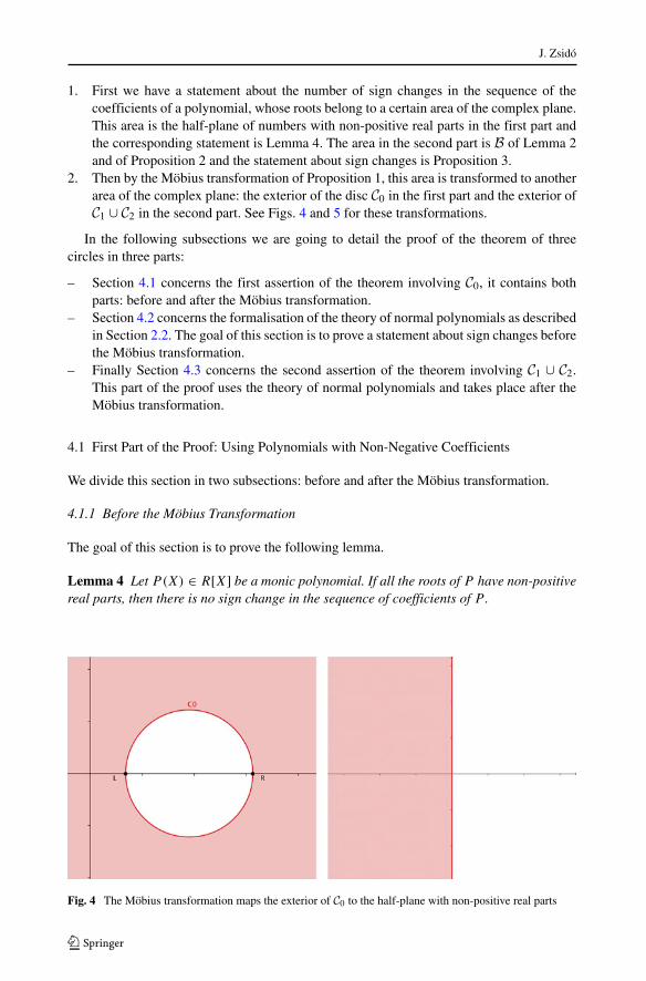
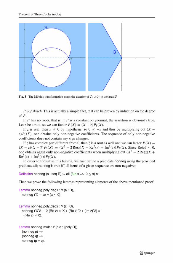
1. First we have a statement about the number of sign changes in the sequence of thecoefficients of a polynomial, whose roots belong to a certain area of the complex plane.This area is the half-plane of numbers with non-positive real parts in the first part andthe corresponding statement is Lemma 4. The area in the second part is B of Lemma 2and of Proposition 2 and the statement about sign changes is Proposition 3.

2. Then by the Mobius transformation of Proposition 1, this area is transformed to anotherarea of the complex plane: the exterior of the disc C0 in the first part and the exterior ofC1 ∪ C2 in the second part. See Figs. 4 and 5 for these transformations.

In the following subsections we are going to detail the proof of the theorem of threecircles in three parts:

– Section 4.1 concerns the first assertion of the theorem involving C0, it contains bothparts: before and after the Mobius transformation.

– Section 4.2 concerns the formalisation of the theory of normal polynomials as describedin Section 2.2. The goal of this section is to prove a statement about sign changes beforethe Mobius transformation.

– Finally Section 4.3 concerns the second assertion of the theorem involving C1 ∪ C2.This part of the proof uses the theory of normal polynomials and takes place after theMobius transformation.

4.1 First Part of the Proof: Using Polynomials with Non-Negative Coefficients

We divide this section in two subsections: before and after the Mobius transformation.

4.1.1 Before the Mobius Transformation

The goal of this section is to prove the following lemma.

Lemma 4 Let P(X) ∈ R[X] be a monic polynomial. If all the roots of P have non-positivereal parts, then there is no sign change in the sequence of coefficients of P .

Fig. 4 The Mobius transformation maps the exterior of C0 to the half-plane with non-positive real parts

Theorem of Three Circles in Coq

Fig. 5 The Mobius transformation maps the exterior of C1 ∪ C2 to the area B

Proof sketch. This is actually a simple fact, that can be proven by induction on the degreeof P .

If P has no roots, that is, if P is a constant polynomial, the assertion is obviously true.Let z be a root, so we can factor P(X) = (X − z)P1(X).

If z is real, then z ≤ 0 by hypothesis, so 0 ≤ −z and thus by multiplying out (X −z)P1(X), one obtains only non-negative coefficients. The sequence of only non-negativecoefficients does not contain any sign changes.

If z has complex part different from 0, then z is a root as well and we can factor P(X) =(X − z)(X − z)P2(X) = (X2 − 2 Re(z)X + Re2(z) + Im2(z))P2(X). Since Re(z) ≤ 0,one obtains again only non-negative coefficients when multiplying out (X2 − 2 Re(z)X +Re2(z) + Im2(z))P2(X).

In order to formalise this lemma, we first define a predicate nonneg using the providedpredicate all; nonneg is true iff all items of a given sequence are non-negative:

Definition nonneg (s : seq R) := all (fun x => 0 ≤ x) s.

Then we prove the following lemmas representing elements of the above mentioned proof:

Lemma nonneg poly deg1 : ∀ (a : R),nonneg (’X − a) = (a ≤ 0).

Lemma nonneg poly deg2 : ∀ (z : C),nonneg (’Xˆ2 − 2 (Re z) ∗ ’X + (Re z)ˆ2 + (Im z)ˆ2) =((Re z) ≤ 0).

Lemma nonneg mulr : ∀ (p q : {poly R}),(nonneg p) →(nonneg q) →nonneg (p ∗ q).

J. Zsido

Lemma nonneg root nonpos : ∀ (p : {poly R}),(p \is monic) →(∀ z : C, root p z →Re z ≤ 0) →nonneg p.

The proof of the last lemma is done by induction on the degree of p as in the proof sketch ofLemma 4. This formal proof contains the largest part of the sketched proof. The remainingtwo lemmas are almost immediate:

Lemma nonneg changes0 : ∀ (s : seq R),(nonneg s) →changes s = 0.

Lemma monic roots changes eq0 : ∀ (p : {poly R}),(p \is monic) →(∀ z : C, root p z →Re z ≤ 0) →changes p = 0.

Having formalised the proof of Lemma 4, we can now turn to the actual assertion of thetheorem involving C0.

4.1.2 After the Mobius Transformation

Explicitly the disc C0 is the area of C = R[i] given by

C0 ={

x + yi ∈ R[i] |(

x − l + r

2

)2

+ y2 <

(r − l

2

)2}

,

or equivalently by

C0 ={x + yi ∈ R[i] | x2 − (l + r)x + y2 + rl < 0

}.

The condition on the roots is that they are in the complementary of C0, so we formalisedirectly the predicate:

Definition notinC (z : C) :=0 ≤ (Re z)ˆ2 − (l + r) ∗ (Re z) + (Im z)ˆ2 + r ∗ l.

By using remark 2, the first part of the assertion is formalised as follows:

Theorem three circles 1 : ∀ (p : {poly R}),(∀ z : C, root p z → notinC z) →changes (Mobius p l r) = 0.

As mentioned before, we want to use Lemma 4 in this proof. In order to apply it, we haveto make sure, that the polynomial we consider is monic. The polynomial (Mobius p l r) is in

Theorem of Three Circles in Coq

general not monic, but we can multiply it with the inverse of its leading coefficient and thisoperation does not affect the sign changes. This fact is formalised by:

Lemma changes mulC : ∀ (p : {poly R}) (a : R),(a �= 0) →changes p = changes (a ∗ p).

So now we can apply lemma monic roots changes eq0, and it remains to prove thatthe roots of (Mobius p l r) all have non-positive real parts. Keeping in mind that this latterpolynomial is in fact Mobius(P(X)) = T−1(Ip(Sr−l (T−l (P (X))))) whose roots all havenon-positive real parts iff the roots of P are in the complement of C0. When keeping trackof the roots during the four transformations, this is what happens: when translating by −l,and then scaling by r − l, the roots are “shifted” into the complement of the circle withdiameter (0, 1). By the following inversion, the complement of the circle is mapped on thehalf–plane with real parts ≤ 1 and by translating this area by −1, we obtain the half–planeof numbers with non-positive real parts. See Fig. 4.

This equivalence is not formalised as such, but is represented by the two lemmas:

Lemma root Mobius C 2 : ∀ (p : {poly R}) (z : C) (l r : R),(z + 1 �=0) →root p ((r + l ∗ z) / (z + 1)) = root (Mobius p l r) z.

and

Lemma notinC Re lt0 2 : ∀ (z : C), (z + 1 �= 0) →(notinC ((r + l ∗ z) / (z + 1))) = (Re z ≤0).

One can see that when applying the above lemmas in the formal proof, the case of a rootin z = −1 is excluded. In fact this case is treated separately, the assertion in this case canbe shown directly since the real part of −1 is non-positive. This completes the formal proofof the first part of the theorem of three circles.

We see that the proof can be formalised basically the same way as the proof on papersuggests, thanks to all the existing theories and tools provided by the Ssreflect library.

4.2 Second Part of the Proof: Formalising Normal Polynomials

This subsection contains the formalisation of Section 2.2 about normal polynomials. Thegoal of this subsection is to prove a statement about sign changes before the Mobiustransformation, Proposition 3.

First we define recursively normal sequences:

Fixpoint normal seq (s : seq R) :=if s is (a::l1) thenif l1 is (b::l2) thenif l2 is (c::l3) then(normal seq l1)&& ((0 = a) || ((a ∗ c ≤ bˆ2) && (0 < a) && (0 < b)))else (0 ≤ a) && (0 < b)

else (0 < a)else false.

Then we qualify a polynomial normal, if its sequence of coefficients is normal:

Definition normal := [qualify p : {poly R} | normal seq p].

J. Zsido

This definition allows us to write p \is normal hereinafter. Then we show several lemmasthat guarantee that our definition of a normal polynomial agrees with the definition fromSection 2.2:

Lemma normal coef geq0 : ∀ (p : {poly R}),(p \is normal) →(∀ k, 0 ≤ p‘ k).

Lemma normal lead coef gt0 : ∀ (p : {poly R}),(p \is normal) →0 < lead coef p.

Lemma normal squares : ∀ (p : {poly R}),(p \is normal) →(∀ k, (1 ≤ k) → p‘ (k.−1) ∗ p‘ (k.+1) ≤p‘ kˆ2).

Lemma normal some coef gt0 : ∀ (p : {poly R}),(p \is normal) →(∀ i, (0 < p‘ i) →(∀ j, (i < j)→ (j < (size p).−1) → 0 < p‘ j)).

Lemma prop normal : ∀ (p : {poly R}),(∀ k, 0 ≤ p‘ k) ∧(0 < lead coef p) ∧(∀ k, (1 ≤ k) → p‘ (k.−1) ∗ p‘ (k.+1) ≤(p‘ k)ˆ2) ∧

(∀ i, (0 < p‘ i) →(∀ j, (i < j)→ (j < (size p).−1) → 0 < p‘ j)) →p \is normal.

Lemma 1 is formalised by:

Lemma monicXsubC normal : ∀ (a : R),(’X − a) \is normal = (a ≤ 0).

The area B is defined by the following predicate:

Definition inB (z : C) :=(Re z ≤ 0) && ((Im z)ˆ2 ≤3 ∗ (Re z)ˆ2).

Lemma 2 is formalised by:

Lemma quad monic normal : ∀ (z : C),((’Xˆ2 − 2 ∗ (Re z) ∗ ’X + (Re z)ˆ2 + (Im z)ˆ2) \is normal)

= (inB z).

The advantage of having formalised normal lists recursively is that in the proofs ofmonicXsubC normal and quad monic normal the normal polynomials are computed by Coqautomatically. Remark 1 is formalised by the lemma:

Lemma normal 0notroot : ∀ (p : {poly R}),(p \is normal) →∼(root p 0) ↔ ∀ k, (k ≤(size p).−1) → 0 < p‘ k.

Theorem of Three Circles in Coq

Lemma 3 is formalised by:

Lemma normal mulr : ∀ (p q : {poly R}),(p \is normal) →(q \is normal) →(p ∗ q) \is normal.

Its proof is done in several steps. First we formalise a restricted version where we haveadditional hypotheses on p and q: 0 is not a root of them. Then we prove that a polynomialP is normal if and only if XnP (X) is normal. Using this, one can factor out Xμp in p, Xμq

in q and Xμp+μq in their product and it suffices to show that pq/Xμp+μq is normal.Now we can formalise Proposition 2:

Lemma normal root inB : ∀ (p : {poly R}),(p \is monic) →(∀ z : C, root p z → inB z) →p \is normal.

Its proof is similar to the one of lemma nonneg root nonpos. The proof goes by inductionon the degree of p. Let z be a root of p so that we can factor p = (X − z)p1(X). If z

is real, then by hypothesis z ≤ 0 and (X − z) is normal by Lemma 1. By the inductionhypothesis p1 is normal. Since the product of two normal polynomials is normal we canconclude that p is normal. If z has non-zero imaginary part, then z is a root too and we canfactor p = (X − z)(X − z)p2(X). By hypothesis z ∈ B and by symmetry z ∈ B too. Thus(X− z)(X− z) is normal by Lemma 2. By the induction hypothesis p2 is normal. Since theproduct of two normal polynomials is normal, we can conclude that p is normal.

Recall from Section 2.2 Proposition 3: it states that the number of sign changes in thesequence of coefficients of P(X)(X − a) is 1, where P is a normal polynomial and a > 0.The formalised Proposition is as follows:

Lemma normal changes : ∀ (a : R) (p : {poly R}),(0 < a) →(p \is normal) →(∼(root p 0)) →changes (seqn0 (p ∗ (’X − a))) = 1.

The hypothesis ∼(root p 0) is justified by Remark 1. For a better readability we introducethe notation n = size (p ∗ (’X − a)).−1. The formal proof of normal changes follows theideas sketched in the proof of Proposition 3 in Section 2.2.

We prove first that (p ∗ (’X − a))‘ 0 < 0 and that 0 < (p ∗ (’X − a))‘ n under the samehypotheses as the ones of normal changes. Then we continue by distinguishing two casesconcerning the length of the sequence of coefficients of p ∗ (’X − a) (which is equivalent todistinguishing by the degree of this polynomial).

If the sequence consists of only two coefficients, then the assertion is immediately true.The sequence cannot consist of less coefficients since p, which is normal, cannot be the zeropolynomial.

The main case is the one where the sequence consists of more than 2 coefficients. In thiscase we can show that the number of sign changes can be decomposed into three terms:

– the number of sign changes between the first and second coefficients,– the number of sign changes between the before last and last coefficients,– the number of sign changes in the middle coefficients.

J. Zsido

This decomposition is formalised by the following lemma:

Lemma changes decomp sizegt2 : ∀ (s : seq R),(all neq0 s) →(2 < size s) →changes s = (s‘ 0 ∗ s‘ 1 < 0) + changes (mid s) +

(s‘ (size s).−2 ∗ s‘ (size s).−1 < 0)

The predicate all neq0 s is true iff all the items of s are different from 0 and the sequencemid s consists of s without the first and last items. We apply changes decomp sizegt2 toseqn0 (p ∗ (’X − a)).

Next we are going to simplify the number of sign changes in the middle coefficients ofseqn0 (p ∗ (’X − a)). Recall from Section 2.2 that the middle coefficients of (p ∗ (’X − a))are of the form p‘ k.+1 ∗ (p‘ k / p‘ k.+1 − a). This sequence can be characterised as the point-wise product of the two sequences (drop 1 p) and a sequence spseq. This latter sequencerepresents the expressions p‘ k / p‘ k.+1 − a and is formalised by

Definition spseq := [seq x.1 / x.2 − a | x <− zip p (drop 1 p)].

The point-wise product of two sequences is formalised by seqmul of typeseq R → seq R → seq R, which takes two sequences as input and returns a sequence whoseitems are products of the corresponding items of the two input lists. So the above mentionedcharacterisation is formalised by the following lemma:

Lemma seqmul spseq dropp : mid (p ∗ (’X −a)) = seqmul spseq(drop 1 p).

Moreover we show that drop 1 p consists of positive items and spseq is increasing, byusing the predicates all pos and increasing:

Lemma all pos dropp : all pos (drop 1 p).

Lemma spseq increasing : increasing spseq.

But since we apply the filter seqn0 on the sequence of the middle coefficients, so thatchanges counts the sign changes correctly, we have to show some technical details due tothe filter.

– The filter seqn0 and mid commute under the condition that the first and last items of asequence are different from zero.

Lemma mid seqn0 C : ∀ (s : seq R),(s‘ 0 �= 0) →(s‘ (size s).−1 �= 0) →mid (seqn0 s) = seqn0 (mid s).

Theorem of Three Circles in Coq

– When examining closely the expressions p‘ k.+1 ∗ (p‘ k / p‘ k.+1 − a), we remark that

pk+1

(pk

pk+1− a

)= 0 ⇔ pk

pk+1− a = 0

because pk > 0 for all coefficients of P . So the items filtered out by seqn0 inmid(p ∗ (’X − a)) are exactly the ones filtered out by seqn0 in spseq. This fact isformalised by the following lemma:

Lemma mid seqn0q decomp : mid (seqn0 (p ∗ (’X − a))) =seqmul (seqn0 spseq)

(mask [seq x �=0 | x <− mid (p ∗ (’X − a))](drop 1 p)).

Furthermore, since (seqn0 spseq) is a subsequence of spseq, it is increasing as well:

Lemma subspseq increasing : increasing (seqn0 spseq)

and since mask [seq x �=0 | x <− mid (p ∗ (’X − a))] (drop 1 p) is a subsequence ofdrop 1 p, all its items are positive:

Lemma subp all pos :all pos (mask [seq x �= 0 | x <− mid (p ∗ (’X − a))] (drop 1 p)).

– Now we are ready to simplify the number of changes in the middle coefficients. Weuse the simple fact that the number of sign changes in a point-wise product of twosequences, where one of the sequences consists of positive items is equal to the numberof sign changes in the other sequence. This fact is given by the lemma

Lemma changes mult : ∀ (s c : seq R),(all pos c) →(size s = size c) →changes (seqmul s c) = changes s.

Summarising the technical lemmas, we obtain thatchanges (seqn0 (mid (p ∗ (’X − a)))) is equal to changes (seqn0 spseq).

Just like in the proof sketch of Proposition 3 in Section 2.2, we show then thatseqn0 spseq has at most 1 sign change since it is increasing.

This fact is formalised for a general increasing sequence by the lemma:

Lemma changes seq incr : ∀ (s : seq R),(increasing s) →(all neq0 s) →(changes s == 1) || (changes s == 0).

J. Zsido

The conclusion of this lemma is a boolean expression, more precisely a boolean disjunc-tion. The boolean disjunction is written || in Ssreflect and the boolean equality is denotedby ==.

Then we proceed by distinction of cases: either 1 or 0 sign changes in seqn0 spseq. Weuse the notation d = size (seqn0 (p ∗ (’X − a))).−1 (and thus d.−1 = size (seqn0 spseq)).

1. First case : changes (seqn0 spseq) = 1. This means that the first item has negative signand the last one positive sign. This is formalised by the lemma

Lemma changes seq incr 1 : ∀ (s : seq R),(1 < size s) →(increasing s) →(all neq0 s) →(changes s == 1) = (s‘ 0 < 0) && (0 < s‘ ((size s).−1)).

The notations of this lemma might seem odd at first sight, since its conclusion is anequality = between two expressions containing another sort of equality ==. The Ssreflectlibraries of Coq are based on manipulating boolean expressions rather than propositionswhere possible. The expression s‘ 0 < 0 for example, is true or false, so is effectivelya boolean. The same is valid for 0 < s‘ ((size s).−1. The operator && is the booleanconjunction. On the left-hand side of the equality the expression changes s == 1 is aboolean expression as well, since it uses boolean equality ==. So the conclusion of thelemma is an equality between boolean expressions.

Applying this lemma to seqn0 spseq, we obtain (seqn0 spseq)‘ 0 < 0 on theone hand which implies that (seqn0 (p ∗ (’X − a)))‘ 0 ∗ (seqn0 (p ∗ (’X − a)))‘ 1 < 0is false. On the other hand we have 0 < (seqn0 spseq)‘ d.−2 which implies that(seqn0 (p ∗ (’X − a)))‘ d.−1 ∗ (seqn0 (p ∗ (’X − a)))‘ d < 0 is false.

So the count of changes according to changes decomp sizegt2 adds up to 1.2. Second case : changes (seqn0 spseq) = 0. This means that the signs of the first and last

items are the same. This is formalised by the lemma:

Lemma changes seq incr 0 : ∀ (s : seq R),(0 < size s) →(increasing s) →(all neq0 s) →((changes s == 0) = (0 < s‘ 0 ∗ s‘ ((size s).−1))).

Again, the assertion is an equality between boolean expressions.So either 0 < (seqn0 spseq)‘ 0 and 0 < (seqn0 spseq)‘ d.−2 or

(seqn0 spseq)‘ 0 < 0 and (seqn0 spseq)‘ d.−2 < 0.If both are positive, then

(seqn0 (p ∗ (’X − a)))‘ 0 ∗ (seqn0 (p ∗ (’X − a)))‘ 1 < 0

is true and

(seqn0 (p ∗ (’X − a)))‘ d.−1 ∗ (seqn0 (p ∗ (’X − a)))‘ d < 0

is false. If both are negative, then

(seqn0 (p ∗ (’X − a)))‘ 0 ∗ (seqn0 (p ∗ (’X − a)))‘ 1 < 0

Theorem of Three Circles in Coq

is false and

(seqn0 (p ∗ (’X − a)))‘ d.−1 ∗ (seqn0 (p ∗ (’X − a)))‘ d < 0

is true.So the count of changes according to changes decomp sizegt2 adds up to 1.

This completes the formal proof of Proposition 3 or of normal changes, as well as the theoryon normal polynomials needed for the proof of the second part.

To summarise, the theory of normal polynomials is not formalised exactly the same waythe informal theory suggests. The inductive definition of normal polynomials leaves com-putations for Coq to conduct. The (informal) proof of Lemma 3 is itself technical and theformal proof of normal mulr is so too, we have not found a way to avoid this. But one canproceed similarly to the informal way thanks to the Ssreflect libraries. For the formal versionof Proposition 3 and its proof (which are normal changes and its proof) the filter seqn0 addstechnical details. They appear in the simplification of changes (seqn0 (mid (p ∗ (’X − a))))to changes (seqn0 spseq) and they do not arise in the informal proof.

4.3 Second Part of the Proof: Using Normal Polynomials

This subsection formalises the part of the proof of the second assertion of the theorem ofthree circles that comes after the Mobius transformation.

First we need to formalise the union of the two disks C1 ∪ C2. They have followingequations: {

x + yi ∈ R[i] |(x − l + r

2

)2 +(y ±

√3(r − l)

6

)2<

(r − l)2

3

},

or equivalently{x + yi ∈ R[i] | x2 − (l + r)x + y2 ±

√3

3(r − l)y + rl < 0

}.

So the union is formalised by the following predicate:

Definition inC12 (l r : R) (z : C) :=((Re z)ˆ2 − (l + r) ∗ (Re z) + (Im z)ˆ2 − (r − l) ∗

(Im z) / (sqrt 3) + l ∗ r < 0) ||((Re z)ˆ2 − (l + r) ∗ (Re z) + (Im z)ˆ2 + (r − l) ∗

(Im z) / (sqrt 3) + l ∗ r < 0).

The second part of the theorem of three circles asserts that if P has exactly one simple rootin C1 ∪ C2, then there is exactly one sign variation in the sequence of Bernstein coefficientsof P . So in fact P is of the form P(X) = (X − a)P (X) where a ∈ (l, r) and a is not a rootof P . This assertion is formalised as follows:

Theorem three circles 2 : ∀ (l r : R) (p : {poly R}) (a : R),(∼(root p r)) →(l < a < r) →(∼(root p a)) →(∀ z : C, root p z →∼ (inC12 l r z) ) →changes (seqn0 (Mobius (p ∗ (’X − a)) l r)) = 1.

The only exotic hypothesis is the one asking for r not to be a root of P . The reason for thisis the fact that we restrict ourselves to the case that 0 is not a root of the normal polynomial

J. Zsido

Mobius (P ) if want to use Proposition 3 or normal changes for the proof. To ask 0 not tobe a root of Mobius(P ) is equivalent of asking for r not to be a root of P .

In order to apply lemma normal changes, first we need to writeMobius(p ∗ (’X − a)) in the form (Mobius p) ∗ (’X − b). By the lemma changes mulC, themultiplication of the sequence by a non-zero constant, such as the inverse of the leadingcoefficient of Mobius (p ∗ (’X −a)), does not affect the sign changes. Furthermore we showthat the Mobius transformation is compatible with the product of polynomials:

Lemma MobiusM : ∀ (p q : {poly R}) (l r : R),Mobius (p ∗ q) l r = (Mobius p l r) ∗ (Mobius q l r).

We can compute explicitly the coefficients of the Mobius transformation of a monicpolynomial of degree 1:

Lemma Mobius Xsubc monic : ∀ (a l r : R),(l �= r) →(l �=a) →(lead coef (Mobius (’X − a) l r))ˆ(−1) ∗(Mobius (’X − a) l r) = ’X + ((r − a) / (l − a)).

Now we can apply lemma normal changes and it remains to show its hypotheses. The firsthypothesis r−a

l−a< 0 can be shown easily since l < a < r .

To show the hypothesis that

(lead coef (Mobius p l r))ˆ(−1) ∗ (Mobius p l r) \is normal,

we apply lemma normal root inB. This polynomial is obviously monic. In order to show thatall the roots of (Mobius p l r) are in B, we show that it is equivalent to ask that all the rootsof p are in the exterior of C1 ∪ C2. We use thus the following lemma

Lemma inB notinC12 : ∀ (l r : R) (z : C),(l �= r) →(z + 1 �= 0) →(inB z) = ∼∼(inC12 l r ((r + l ∗ z) / (z + 1)))

together with lemma root Mobius C 2 from Section 4.1. The conclusion of lemmainB notinC12 is an equality of boolean expressions using the boolean negation, denoted by∼∼.

So we have obtained the equivalence between “all roots of (Mobius p l r) are in B” and“all roots of p are in the exterior of C1 ∪ C2”.

What happens here is intuitively similar to Section 4.1. We keep track of the complemen-tary area of C1 ∪ C2 when doing the Mobius transformation: translation by −l, then scalingby r − l, inversion and translation by −1.

The computations are not as immediate as in Section 4.1, but lemma inB notinC12 provesthe correctness. The case of a root in z = −1 has to be treated apart, but without any furtherdifficulty. This concludes the formal proof of the second assertion.

This part of the proof can be formalised the way that the informal counterpart suggests.

5 Discussion and Future Work

First we would like to mention some technical remarks concerning the formalisation theway it was carried out.

Theorem of Three Circles in Coq

We implemented normal polynomials recursively because in the proofs ofmonicXsubC normal and quad monic normal the computations are carried out automaticallyby Coq. Whereas in an alternative definition by a (rather cumbersome) predicate, one wouldhave to show “by hand” the four defining properties. A simplification of normal polynomi-als, considering remark 1, would have been to formalise only normal polynomials withoutany root in 0, since in almost all proofs thereafter, we add this hypothesis.

As mentioned in the introduction, one of our motivations for formalising the theoremof three circles is to provide the main pieces for the formal proof of the termination of thealgorithm of real root isolation as described in [1]. The next step is to construct a formalmodel of the algorithm and make it executable, either inside the Coq system or by extractingexecutable Ocaml or Haskell code [15]. We plan to use the CoqEAL for effective algebraand the refinement techniques outlined in [8] for this task, but preliminary experimentssuggest that this refinement technique requires improvements in our case, especially sincecomputations would be performed with rational numbers, but proofs are performed in realclosed field (a field where the intermediate value theorem is valid for polynomials, whichis not the case for rational numbers).

Another one of our motivations for formalising the theorem of three circles is to formalisethe general case involving Obreshkoff areas and lenses. Chapter two of [9] explains allthe details, presenting the relevant works of Obreshkoff. Lemmas nonneg changes0 and3, or its formalised version normal changes, are generalised by the following theorem ofObreshkoff (restated in [9] as Theorem 2.7)

Theorem 2 (Obreshkoff) Consider the real polynomial P(X) = ∑ni=0 aiX

i of degree n

and its complex roots, counted with multiplicities. Let v denote the number of sign changesof the sequence (a0, . . . , an). If P(X) has at least p roots with arguments in the range− π

n+2−p< ϕ < π

n+2−p, and at least n − q roots with arguments in the range π − π

q+2 ≤ψ ≤ π + π

q+2 , then p ≤ v ≤ p. If p = q, then P(X) has exactly p roots with arguments ϕ

in the range given above and v = p.

The special case p = q = 0 is our lemma noneg changes0: the range for ψ is[

π2 ; 3π

2

],

which corresponds to roots with non-positive real part.The special case p = q = 1 is our Lemma 3 or normal changes: the range for ψ

is[

2π3 ; 4π

3

]which corresponds to the area B and one complex root (without its complex

conjugate) with argument in the range(− π

n+1 ; πn+1

)implies that this root is in fact real and

positive.The transformation of polynomials from Proposition 1 in order to obtain the Mobius

transform or Mobius p is characterised in [9] as the Mobius transformation I of the interval(0,∞) to an arbitrary open interval (l, r):

P(X) �→ (X + 1)nP

(r + lX

X + 1

)

which is the transformation we use in lemma root Mobius C 2 (as well as in notinC Re lt0 2and inB notinC12). This is our reason for calling the sequence of the four transformations inProposition 1 a Mobius transformation.

The generalisation of the theorem of three circles is obtained by transferring Theorem 2to an arbitrary interval (l, r). To do so we define first Obreshkoff areas and lenses.

J. Zsido

The two Obreshkoff discs Ck and Ck for an integer k are the open discs whose delimitingcircles touch the endpoints of (l, r) and whose centers see the line segment (l, r) under theangle 2π

k+2 . The Obreshkoff area Ak is the union Ck ∪ Ck and the Obreshkoff lens Lk is the

intersection Ck ∩ Ck .

Theorem 3 (Obreshkoff) Consider the real polynomial P(X) of degree n and its roots inthe complex plane, counted with multiplicities. Let v denote the number of sign changes inthe sequence of coefficients of the Mobius transformation of P to the interval (l, r). If P

has at least p roots in the Oreshkoff lens Ln−p and at most q roots in the Obreshkoff areaAq , then p ≤ v ≤ q.

The assertions of the theorem of three circles are the special cases of p = q = 0 andp = q = 1.

In order to formalise these two Theorems 2 and 3, one would have to make the followingchanges (at least) in the definitions of the structures needed for the proofs.

– Adapt the definition of the discs C1 and C2 to Obreshkoff areas with at least one integerparameter. Formalise Obreshkoff lenses.

– Adapt the definition of the area B, with at least one more parameter, define the areacorresponding to the angle range for ϕ.

– Adapt the definition of normal polynomial with respect to the parametrised version ofB. If possible keep recursive definition, in order to make computations automatic whenpossible.

To carry out the proof of Theorem 2, one would have to prove first the special caseq = n. This proof could be done in two steps: first an analogous lemma to normal root inB,with a proof by induction on the degree of the polynomial P , and then an analogous one tonormal changes which provides an upper bound for the number of sign changes rather thanan exact number of changes. Then with this special case one can prove the general statementof Theorem 2 by applying the special case to P(X) and P(−X).

To prove Theorem 3, we need first the mentioned Mobius transformation. For this pur-pose lemma root Mobius C 2 together with a similar lemma to inB notinC12 are mostlyenough. The proof of Theorem 3 would be then quite analogous to the one of three circles 2.

Bearing in mind that our work provides tools for the formalisation of correctness of theNewDsc algorithm for example, we would have accomplished the first step in this direction.But until the completion of this goal, we still have many opportunities for exploration offormalisation of mathematical theories.

References

1. Basu, S., Pollack, R., Roy, M.F.: Algorithms in real algebraic geometry. In: Algorithms and Computationin Mathematics, vol. 10, 2nd edn. Springer-Verlag, Berlin (2006)

2. Bertot, Y., Casteran, P.: Interactive theorem proving and program development. In: Texts in TheoreticalComputer Science. An EATCS Series. Springer-Verlag, Berlin (2004). Coq’Art: the calculus of inductiveconstructions, With a foreword by Gerard Huet and Christine Paulin-Mohring

3. Bertot, Y., Guilhot, F., Mahboubi, A.: A formal study of Bernstein coefficients and polynomials. Math.Struct. Comput. Sci. 21(4), 731–761 (2011)

4. Cohen, C.: Formalized Algebraic Numbers: Construction and First Order Theory. Ph.D. thesis, Ecolepolytechnique, France (2012)

Theorem of Three Circles in Coq

5. Cohen, C., Mahboubi, A.: Formal proofs in real algebraic geometry: from ordered fields to quantifierelimination. Log. Methods Comput. Sci. 8(1) (2012)

6. Coq Development Team, T.: The Coq Proof Assistant. http://coq.inria.fr7. Coq Development Team, T.: The Coq Proof Assistant Reference Manual—Version V8.4. http://coq.inria.

fr (2012)8. Denes, M., Mortberg, A., Siles, V.: A refinement-based approach to computational algebra in coq. In:

Beringer, L., Felty, A.P. (eds.) ITP, Lecture Notes in Computer Science, vol. 7406, pp. 83–98. Springer(2012)

9. Eigenwillig, A.: Real Root Isolation for Exact and Approximate Polynomials using Descartes’ Rule ofSigns. Ph.D. thesis, Universitat des Saarlandes, Germany (2008)

10. Flyspeck: Thomas C. Hales, Project Leader: The Flypseck Project. NSA grant 0804189. https://code.google.com/p/flyspeck/

11. ForMath: Thierry Coquand, Project Leader: The ForMath Project. EU FP7 STREP FET, grant agree-ment nr. 243847, March 2010–February 2013. http://wiki.portal.chalmers.se/cse/pmwiki.php/ForMath/ForMath

12. Gonthier, G., Mahboubi, A.: An introduction to small scale reflection. Coq. J. Formalized Reason. 3(2),95–152 (2010)

13. Hales, T.C., Harrison, J., McLaughlin, S., Nipkow, T., Obua, S., Zumkeller, R.: A revision of the proofof the kepler conjecture. Discret. Comput. Geom. 44(1), 1–34 (2010)

14. Kerber, M., Sagraloff, M.: Efficient real root approximation. In: Schost, E., Emiris, I.Z. (eds.) ISSAC,pp. 209–216. ACM (2011)

15. Letouzey, P.: A new extraction for coq. In: Geuvers, H., Wiedijk, F. (eds.) TYPES, Lecture Notes inComputer Science, vol. 2646, pp. 200–219. Springer (2002)

16. Mahboubi, A.: Contributions a la certification des calculs dans R: theorie, preuves, programmation.These, Universite de Nice Sophia-Antipolis. http://hal.inria.fr/tel-00117409 (2006)

17. Mahboubi, A.: Programming and certifying a CAD algorithm in the Coq system. In: Dagstuhl Semi-nar 05021—Mathematics, Algorithms, Proofs. Dagstuhl Online Research Publication Server, Dagstuhl.http://hal.inria.fr/hal-00819492 (2006)

18. Mahboubi, A.: Implementing the cylindrical algebraic decomposition within the Coq system. Math.Structures Comput. Sci. 17(1), 99–127 (2007). doi:10.1017/S096012950600586X

19. Mehlhorn, K., Sagraloff, M.: Isolating real roots of real polynomials. In: Johnson, J.R., Park, H.,Kaltofen, E. (eds.) ISSAC, pp. 247–254. ACM (2009)

20. Munoz, C.A., Narkawicz, A.: Formalization of bernstein polynomials and applications to globaloptimization. J. Autom. Reason. 51(2), 151–196 (2013)

21. Sagraloff, M.: When Newton meets Descartes: a simple and fast algorithm to isolate the real roots of apolynomial. In: van der Hoeven, J., van Hoeij, M. (eds.) ISSAC, pp. 297–304. ACM (2012)

22. Ssreflect: The Mathematical Components Project: Ssreflect Extension and Libraries. http://www.msr-inria.com/projects/mathematical-components

23. Zumkeller, R.: Global Optimization in Type Theory. These, Ecole Polytechnique. http://www.alcave.net(2008)