The costs and benefits of symmetry in

common-ownership allocation problems∗

Alexander L. Brown† and Rodrigo A. Velez‡

Department of Economics, Texas A&M University, College Station, TX 77843

July 12, 2015

Abstract

In experimental partnership dissolution problems with complete information,the divide-and-choose mechanism is significantly superior to the winner’s-bid auc-tion. The performance of divide-and-choose is mainly affected by reciprocity is-sues and not by bounded rationality. The performance of the winner’s-bid auctionis significantly affected by bounded rationality. Contrary to theoretical predictionsdivide-and-choose exhibits no first-mover bias.

JEL classification: C91, D63, C72.

Keywords: experimental economics; no-envy; divide-and-choose; winner’s-bidauction; behavioral mechanism design.

1 Introduction

We experimentally study mechanisms for the allocation of an indivisible good amongtwo agents when ownership of the good is symmetric and compensation with an in-finitely divisible good, e.g., money, is possible. Examples are a partnership dissolution(Cramton et al., 1987), a divorce settlement (McAfee, 1992), and the allocation of ballpossession in National Football League overtime (Che and Hendershott, 2008). We as-sume complete information, i.e., agents know each other well—more on this key as-sumption below. We experimentally compare the performance of two prominent mech-anisms: the winner’s-bid auction (Cramton et al., 1987), a simultaneous move mech-anism, and the popular divide-and-choose (McAfee, 1992), a sequential move mecha-nism. Over all measures, divide-and-choose is superior to winner’s-bid auction. The

∗Thanks to an associate editor, two anonymous referees, Catherine Eckel, John Van Huyck, and audi-ences at the 2010 and 2011 North American ESA Meetings, SCW2012, XIII JOLATE, 2013 World ESA Meetings,CRETE2014 and seminar presentations at the U. of Alabama, Texas A&M, U. C. Santa Barbara, Chapman U.,and the U. of Sydney for valuable comments and discussions. Special thanks to Jacob Williams and YueZhang for transcribing survey data from experiments. All errors are our own.

†abrown@econmail.tamu.edu; http://econweb.tamu.edu/abrown‡rvelezca@econmail.tamu.edu; https://sites.google.com/site/rodrigoavelezswebpage/home

1

performance of the winner’s-bid auction is affected mainly by subject’s bounded ratio-nality and not by coordination failure. Divide-and-choose is affected by reciprocity is-sues and not by a lack of subject’s sequential rationality. Contrary to theoretical predic-tions, divide-and-choose gives no advantage to the first-mover.

Our study will likely impact the practice of fair division. In particular, our results in-form smartphone and computer applications that are currently attempting to provideusers with arbitration mechanisms to solve the type of allocation problems we considerin our study (e.g., Fair Outcomes Inc., 2007-2013; Splitwise Inc., 2014; and Spliddit, 2014).Some of these mechanisms theoretically deliver desirable outcomes. However, theorydoes not allow one to differentiate them from competing proposals. Our experimentalstudy fills this need. We are able to document sharp differences in the performance, ina laboratory environment, of some of the most prominent mechanism available. Be-havioral biases exhibited by subjects in our experiments, affect different mechanisms indifferent degrees. As a consequence, theoretically equivalent mechanisms, turn out tobe significantly different in practice. Curiously, none of the services cited above offersour best performing mechanism.1 Our results also open the possibility to design nor-matively compelling mechanisms that minimize the effect on their performance of thebehavioral biases that we observe (Sec. 5).

We frame our experiments as the allocation of a social endowment of two indivisiblegoods, “items,” among two agents, each agent receives exactly one item, and there is thepossibility of monetary compensation. This is an equivalent formulation of the alloca-tion of a single indivisible good with monetary compensation. We find our environmentmore appropriate for our experimental setting. Having two items allows us to avoid, tosome extent, agents’ non-monetary incentives to “win” items, which is documented inauction settings (e.g., Cooper and Fang, 2008; Roider and Schmitz, 2012) —notice thatour results also inform the allocation of rooms and division of rent among two room-mates who collectively lease an apartment (Abdulkadiroglu et al., 2004). For simplicityof exposition in this introduction, we use the language of allocation of a single good.

Complete information is a relevant benchmark for situations like the dissolution ofa long standing partnership or a marriage. When agents know each other well, their ac-tions in the “game” induced by an allocation mechanism convey their intentions. Whenthese intentions are revealed in a game, reciprocity issues systematically affect agents’behavior (see Charness and Rabin, 2002, among many others). More importantly, theseissues can have a different effect in competing mechanisms (Andreoni et al., 2007).2

We concentrate on the evaluation of these differential effects and implement a com-plete information environment in the laboratory. Our results confirm that they are rele-

1In Sec. 5 we discuss the relevance of our results for the mechanisms used by Fair Outcomes Inc. (2007-2013) and Spliddit (2014). Splitwise Inc. (2014) offers allocation of rent and rooms among roommates basedon surveys of preferences over the verifiable features of rooms like size, number of windows, etc., not theactual preferences of the agents in the division problem.

2In a seller-buyers auction setting, as information structure becomes closer to complete information, thespite motive considerably affects the outcomes of the second-price auction, but not the first-price auction.

2

vant and have to be taken into consideration when designing mechanisms for common-ownership distributive situations in which one expects agents will know each other well.

We evaluate our mechanisms with two criteria. First is efficiency, i.e., an agent whovalues the object the most receives it. Second is equity. Here, we evaluate whether theallocation obtained can be sustained as the outcome of a market in which both agentshave an equal share of the aggregate income. These allocations, which we refer to asequal-income market allocations, are arguably the most normatively compelling in ourenvironment (Thomson, 2010; Varian, 1976). They not only are efficient, but also, in ourenvironment, they coincide with the set of envy-free allocations, i.e., those at which noagent prefers the allotment of the other agent to her own. They can be easily describedas follows. An agent who values the object the most receives it and transfers the otheragent an amount between half the low-value agent’s value and half of the high-valueagent’s value. Thus, the set is isomorphic to an interval. Between two allocations in thisinterval the low-value agent prefers the allocation on the right and the high-value agentprefers the allocation on the left (Sec. 2).

We evaluate the performance of two of the most prominent mechanisms that theo-retically obtain equal-income market outcomes among strategic rational agents. Ourfirst mechanism, the winner’s-bid auction, operates as follows: both agents simulta-neously bid for the object; then, an agent with the highest bid receives the object andpays her bid to the other agent. The set of Nash equilibria of the game induced by thismechanism for some given valuation structure is the set of equal-income market allo-cations with respect to the true preferences (Sec. 2.2). Our second mechanism, divide-and-choose, operates as follows: a randomly selected first-mover, which we refer to as“divider,” proposes a transfer from the agent who receives the object to the other agent;then the second-mover, which we refer to as “chooser,” decides whether to get the ob-ject and make the proposed transfer or to give up the object and get the transfer. Theoutcome in sub-game perfect equilibria of the game induced by this mechanism is thedivider’s preferred equal-income market outcome for the true values (Sec. 2.2).

Both mechanisms we evaluate are intended to provide a form of end-state justice,for their equilibrium outcomes are equal-income market allocations. One can arguethat divide-and-choose lacks procedural justice, however (Moulin, 2006). After dividerand chooser are selected, the mechanism not only loses symmetry, but also gives the di-vider a considerable advantage. Thus, theory provides a clear benchmark for the evalua-tion of these mechanisms: (i) the winner’s-bid auction should provide an equal-incomemarket allocation, free of any bias predetermined by the mechanism designer; and (ii)divide-and-choose should provide an equal-income market allocation that is biased to-wards the divider. Our study is the first to evaluate the extent to which this normativeranking based on equilibrium predictions is realized in an experimental environment.

Our first result is that divide-and-choose is superior to winner’s-bid auction over allmeasures. Divide-and-choose obtains 81% equal-income market allocations and 85%efficient allocations. The more procedurally fair winner’s-bid auction obtains 41% equal-income market allocations and 73% efficient allocations. The differences are statistically

3

significant. Our second result is that the winner’s-bid auction is affected by subjectsunderbidding and not by coordination failure. Symmetry turns out to be a costly fea-ture for this mechanism. Among boundedly rational players, as in our experiments, itinduces a distortion caused by the simultaneity of play. Our data suggest that this distor-tion slowly improves over time, but does not improve to the level of divide-and-choose.This result points in a precise direction for the improvement of the winner’s-bid auction(Sec. 5). Our third result is that divide-and-choose is affected mainly by reciprocity is-sues. Even though divide-and-choose performs better than the winner’s-bid auction, itobtains inefficient allocations with positive probability. Essentially, in the sub-game per-fect equilibrium of the divide-and-choose game, the chooser is nearly indifferent amongthe bundles selected by the divider. Thus, when the divider selects a proposal that isclose to the sub-game perfect one, the chooser may choose the inefficient allocation andget almost the same payoff that she would obtain with her best response. This “rejectionstrategy” induces a considerable loss for the divider and is responsible for the majorityof inefficient outcomes. This suggests that the mechanism may be improved by return-ing some symmetry without losing the sequentiality of play (Sec. 5). Our fourth result isthat the divide-and-choose mechanism, contrary to theoretical predictions, exhibits nofirst-mover advantage. Indeed, if at all, there is a second-mover advantage. Finally, ourfifth result compares payoffs for different roles in our mechanisms. First, the efficiencygains achieved by the divide-and-choose mechanism over the winner’s-bid auction arerealized mainly for low-value and second-mover subjects. Second, there is no significantloss for high-value first-mover subjects in the divide-and-choose mechanism comparedto the winner’s-bid auction. This implies that “behind the veil of ignorance,” the divide-and-choose mechanism dominates the winner’s-bid auction.

There is relatively little experimental work in the area of common-ownership prob-lems under complete information. Guth et al. (1982) study the outcomes of the divide-and-choose mechanism for the allocation of a set of indivisible “chips” that have differ-ent value for divider and chooser.3 Their results are qualitatively consistent with ours;they observe responders’ willingness to reject proposals. Our experimental design dif-fers in two dimensions. First, in our experiments subjects can propose arbitrary trans-fers and thus divide-and-choose results can be compared with those of the winner’s-bidauction. This comparison is a central contribution of our paper. Second, in our ex-periments for the divide-and-choose mechanism, the role of the divider is randomly as-signed among all subjects as opposed to being assigned among high-value agents only asin Guth et al. (1982). Thus, our experiment can answer the question whether the second-movers in divide-and-choose are more prone to reject inequality increasing proposalsthat have low rejection cost (only available to low-value second-movers) than equalitygenerating proposals that have low rejection cost (only available to high-value second-movers). Finally, since in our experiment both high-value and low-value agents get to befirst and second movers, we are able to evaluate the first-mover bias of the mechanism.In Guth et al. (1982) it is not clear whether differences in earnings should be attributed

3Guth et al. (1982) refer to the divide-and-choose games as “complicated ultimatum games.”

4

to divider bias or valuation structure. Herreiner and Puppe (2009) investigate whetherequal-income market allocations result from an “infinitely many proposals” bargain-ing mechanism under a time limit. They document that this mechanism achieves fewequal-income market allocations. However, it is difficult to interpret these results, forit is not clear that Nash equilibrium outcomes of this bargaining procedure are equal-income market allocations. Schneider and Krämer (2004) and Dupuis-Roy and Gosselin(2009, 2011) experimentally evaluate the performance of the divide-and-choose mech-anism. However, in their environment, monetary compensation is not possible. Thus,their experiments are silent about the performance of this mechanism in the distribu-tive situations that motivate our study. Finally, in an incomplete information settingKittsteiner et al. (2012) compared the performance of the winner’s-bid auction and thedivide-and-choose mechanism. The result there is that divide-and-choose weakly dom-inates the auction in terms of percentage of efficient allocations achieved in laboratoryexperiments. However, the difference is not large and only weakly statistically signifi-cant. Our results show that when players know each other well, the difference in perfor-mance is substantial and significant.

The remainder of the paper is organized as follows. Section 2 introduces the modeland mechanisms we study. Section 3 presents our experimental design. Section 4 presentsour results. Section 5 discusses our results and concludes.

2 Model

2.1 environment

We consider two agents, {1,2}, who collectively own two indivisible goods, {A, B}, whichwe refer to as items. Each agent receives one item and either transfers or receives anamount of money to or from the other agent. The value that agent i ∈ {1,2} assignsto item α ∈ {A, B} is v αi . We normalize the value of item A to be 100 for each agent.Agent i ’s utility of receiving item α and transferring an amount x i ∈R to the other agentis u i (x ,α) = v αi −x i (when x i < 0, agent i receives |x i | from the other agent). We assumebudget balance, so x1+x2 = 0.

It is convenient for our purpose to keep track of each agent’s net value of item B , i.e.,the amount of money x B

i such that v Bi − x B

i = v Ai + x B

i (agent i is indifferent betweenpaying x B

i for B or receiving A and being paid x Bi ). Since we normalize v A

i = 100, thenx B

i = (vBi − 100)/2. Clearly, having the higher value of item B is equivalent to having the

higher net value of item B . Let x B =min{x B1 ,x B

2 } and x B =max{x B1 ,x B

2 }. We refer to anagent with the maximal value of item B as a high-value agent and to an agent with theminimal value of item B as a low-value agent.

An allocation is efficient if there is no other allocation that both agents weakly preferand at least one agent strictly prefers. These allocations are those at which a high-valueagent receives item B . One can graphically represent them by means of the transfer from

5

the agent who receives item B , i.e., a high-value agent, to the other agent (Figure 1). Werefer to the difference max{v B

1 ,v B2 }−min{v B

1 ,v B2 } as the efficiency surplus.

We are interested in the set of equal-income market allocations. That is, there areprices pA and p B for the items; each agent has an income pA+p B

2and chooses between

buying A at pA or buying B at p B ; and market clears. These allocations were proposedby Foley (1967) in order to achieve no-envy, i.e., that no agent prefers the allotment ofthe other agent to her own. In our environment equal-income market allocations areefficient and coincide with the set of envy-free allocations (Svensson, 1983). One caneasily characterize them by using the no envy conditions (1 does not envy 2 and viceversa) as the efficient allocations at which the agent who receives item B transfers anamount to the other agent in the interval [x B ,x B ] (Figure 1). We follow Tadenuma andThomson (1995b) and refer to the length of the set of equal-income market transfers, i.e.,x B −x B , as the equity surplus. The equity surplus is half of the efficiency surplus.

2.2 Mechanisms implementing equal-income market allocations

We are interested in experimentally testing mechanisms to obtain equal-income marketallocations. No mechanism does so in dominant strategies (Tadenuma and Thomson,1995a). However, mechanisms that do so with respect to other non-cooperative predic-tions exist. The following, which have been focal in the literature on partnership disso-lution, achieve this (Cramton et al., 1987; McAfee, 1992).4

Winner’s-bid auction: Both agents simultaneousy bid for item B (bids can be nega-tive). An agent with a highest bid receives item B and transfers her bid to the other agent,who receives item A and the transfer. In our experimental setting we break ties in favorof an agent with true higher value for item B .

The set of pure-strategy Nash equilibrium outcomes of the game induced by ourwinner’s-bid auction, i.e., the one in which we break ties in favor of the true high-valueagent, is exactly the set of market allocations (Figure 1). In equilibrium both agents re-port equal bids in the interval [x B ,x B ].5 Intuitively, agents will not coordinate on aninefficient allocation because in that case there is always an agent who prefers the con-sumption of the other agent. By bidding just above or below the other agent, an agent

4It is also relevant to consider the possibility that a mechanism whose non-cooperative equilibrium out-comes are not market allocations may produce them because of the behavioral deviations that agents usu-ally exhibit in the laboratory. With this purpose we also run experiments with the popular ultimatum bar-gaining, which we do not report in this paper. It turns out that both divide-and-choose and winner’s-bidauction perform significantly better than ultimatum bargaining in terms of the percentage of equal-incomemarket allocations obtained and ultimatum bargaining is significantly biased towards the first mover.

5This characterization applies also to an environment with integer bids as in our experiment. Dependingon the way one breaks ties when bids are equal, the bidding game induced by the winner’s-bid auction mayhave no pure-strategy Nash equilibria when bids are not restricted to integer amounts. A sensible predic-tion for these games, that intuitively bypasses the role of the tie-breaker, is limit equilibria (Radner, 1980).Independently of the tie breaker, if preferences are quasi-linear, the set of limit equilibrium outcomes of thewinner’s-bid auction is again the set of equal-income market allocations with respect to true preferences(Velez, 2015).

6

[ ][ ] t B

x Bx

B−100 max{v B1 , v B

2 }

- equal-income market allocations

- winner’s-bid auction pure-strategy Nash equilibrium outcomes

b b

- divide-and-choose sub-game perfect Nash equilibrium outcomes

divider has high value on item B

divider has low value on item B

Figure 1: Efficient allocations, market allocations, and non-cooperative equilibrium outcomes from

popular mechanisms. At each efficient allocation a high-value agent receives item B . Thus, these allo-cations can be graphically represented by means of t B , the transfer from the agent who receives B to theother agent.

can essentially guarantee to obtain the other agent’s allotment. A high-value agent willnever bid more than x B and receive B . Otherwise, she could just bid x B and either payless for B or let the other agent get B and transfer her no less than x B . A low-value agentwill never receive A and a transfer to the left of x B . Otherwise, she could just bid x B ,get B , and transfer x B to the other agent.6 Consistent with this characterization of Nashequilibria for this mechanism, we refer to a bid that is less than x B as a below-Nash bid;to a bid in the interval [x B ,x B ] as a Nash bid; and to a bid greater than x B as an above-

Nash bid.

Divide-and-choose. A randomly selected agent, the divider, names a transfert B ∈ R. The other agent, the chooser, selects either to get item B and transfer t B to thedivider, or to get item A and receive t B from the divider. The divider receives the residualallotment.

A sensible prediction for the sequential game induced by the divide-and-choose me-chanism for utility maximizing agents is sub-game perfect equilibria. Standard argu-ments show that if a high-value agent is the divider, in the equilibrium path, she pro-poses x B and the chooser selects to get item A and receive x B from the divider. Symmet-rically, if the divider is the low-value agent, in the equilibrium path, she proposes x B andthe chooser selects to get item B and transfer x B to the divider (Figure 1).7

Table 1 summarizes the two mechanisms that we experimentally study. The winner’s-bid auction is symmetric, i.e., in its induced game each agent has the same action space.It achieves in non-cooperative equilibria equal-income market allocations, which areefficient. The equilibria of the winner’s-bid auction game requires agents coordination.Since it is a simultaneous move game, no agent ever replies to the action of another

6See our discussion of Result 2 in Sec. 4 for a description of mixed-strategy equilibria in the winner’s-bidauction.

7With integer bids there are two additional equilibrium outcomes when x B > x B . A high-value proposermay propose x B+1 and the low-value chooser selects to receive A. A low-value proposer may propose x

B−1

and the high-value chooser selects to receive B .

7

Mechanism EfficientEqual-income

marketallocations

SymmetricCoordination

requiredReciprocity

issues

Winner’s-bid auction yes yes yes yes noDivide-and-choose yes yes no no yes

Table 1: Properties of mechanisms we experimentally evaluate. The winner’s-bid auction is the onlymechanism to satisfy three normative theoretical properties. Because of its simultaneity, it is also the onlymechanism to require coordination.

player and is affected by the perceived intention of that action. Thus, one can expect thatreciprocity is not an important source of deviations from Nash behavior. The divide-and-choose mechanism achieves in sub-game perfect Nash equilibria equal-income marketallocations, which are efficient. After the divider is determined, the induced game is notsymmetric. Since the game is sequential, it requires no coordination of players. More-over, the chooser’s action may be affected by the perception of the divider’s intentions.

3 Experimental Design and Procedures

We implement the environment and mechanisms described in Sec. 2. Subjects, ran-domly selected each round into groups of two, chose how to allocate two indivisibleitems with possible transfer payments.8 In all possible allocations, each subject receivedexactly one item. Each period, subjects received points for acquiring an item, equal totheir value of that item. Thus, the values for each item are induced values.

The experiment consisted of 50 periods, with 5 different valuations occurring se-quentially over 10 consecutive periods each. For any period, for each grouping of sub-jects, one subject was randomly assigned the high value on item B , the other was as-signed the low value on item B . Thus a subject’s value on item B could change for anyperiod, but the valuation structure (the high and low values for item B ) remained thesame for the 10 periods. Subjects always valued item A at 100. In order of appearance,the pairing of subject values for item B were (40,80), (120,160), (40,120), (160,160), and(0,40).9 Table 2 provides an example of a valuation structure, the third used in the exper-iments. Here, both subjects have the same value for item A, but their values for item B

are different: player 1 has the high value for item B (120 points), and player 2 has the lowvalue for item B (40 points).

8We chose to have subjects bid over two items to match the generalized theoretical environment moreclosely and reduce the possibility that of subjects are motivated by the non-monetary desire to “win” anitem (e.g., Cooper and Fang, 2008; Roider and Schmitz, 2012).

9The ordering of the valuations was chosen at random, but remained constant across both mechanisms.The valuations were specifically chosen to allow for two possibilities where both players value item A morethan B (40, 80) and (0, 40), two possibilities where both players value item B more than A (120, 160) and(160, 160), and one where one player one player values B more than A and one values A more than B

(40, 120). Additionally the fourth valuation (160, 160) was chosen to allow an environment where there isone unique equilibria over all three mechanisms, and coordination should not be an issue.

8

PlayerValue ofItem A

Value ofitem B

Player 1 100 120Player 2 100 40

Table 2: A sample valuation. In this valuation, one subject valued item A at 100 and item B at 120. As inour theoretical environment, the other subject with whom she is paired had the same value for item A, butvalued item B at 80. Each player had an equal chance of receiving the high value on item B for any period.Values were common knowledge to both players. This specific valuation structure (“valuation 3”) was usedfor periods 21–30.

To avoid incentives associated with repeated play, subjects were randomly re-assignedto each other at the beginning of each period. Subjects were instructed that they were tobe randomly rematched each period, and no identifying information (e.g., subject num-ber) was disclosed to a subject about her match in any round. Each period began witheach subject seeing the valuation structure for the period.

3.1 Winner’s-bid auction

In the winner’s-bid auction session, after observing the valuation structure for the pe-riod, subjects simultaneously submitted their bids for item B . The subject with thehigher bid received item B , and the subject with the lower bid received item A. In thisway, the winner’s-bid auction is a first-price auction to acquire item B over item A. In thecase of equal bids, the subject with the higher value of item B received item B .10 Thesubject who received item B , then paid the subject who received item A the full amountof her bid.11

After submitting a bid, each subject was allowed to submit a possible value for theother player’s bid. The experimental software then displayed the outcome (i.e., who getswhich item, what amount is transferred for each player, each players’ earnings for thatperiod) that would occur with those two bids as well as a table that showed all possibili-ties that could happen if the other player’s bid were below, equal to, or above the subject’sbid (see Figure 2). After a subject viewed these possibilities, she could chose to confirmher bid, or chose an alternate bid. If she chose an alternate bid, the process repeated.The process ended when a subject confirmed her bid.

After both subjects submitted their bids, they were asked to guess what they believed

10In the case of the fourth valuation where both subjects value item B at 160, one subject was randomlyselected to win ties, this was known before bids were submitted (i.e., ex-ante). The tie-breaking rules werechosen to allow for easier analysis of equilibrium.

11To eliminate the possibility of grossly negative earnings, bids were restricted so that no bid could belower than the opposite of twice the value of item A (-200, always) and no bid could be higher the twice themaximum value of item B (varies by valuation, i.e, 160, 320, 240, 320, and 80 for each valuation, respec-tively). Of the 1200 observed bids in the winner’s-bid auction, 11 were at the bid minimum and 0 were atthe bid maximum.

9

Figure 2: Confirmation screen for subjects. Subjects have the option to review their bid and the possibleoutcomes associated with it after submitting their initial bid.

was the other subject’s bid.12 If they guessed correctly they received a small bonus of 5points. The value of this bonus was deliberately chosen to be small, so that subjects didnot alter their bidding strategy to receive the bonus. After both subjects submitted theirguesses they saw the outcome of their bidding. They learned what the other player bid,which items they both received, the transfer payment between them, their earnings, andtheir partners’ points earned. Subjects learned if they received a bonus for guessing theother player’s bid correctly, but did not learn if the other player had received the bonusfor guessing their bid correctly. After this information was disclosed, a new period began.This process continued for 50 periods.

12Subject guesses appear to be unrelated any other part of their behavior. The data are not meaningfuland not presented here. Subjects are clearly not best responding to their guesses; this result is consistentwith Costa-Gomes and Weizsäcker (2008) who study this issue in detail.

10

3.2 Divide-and-choose

In the divide-and-choose session, at the beginning of each period, one subject was ran-domly selected to be the divider. That subject chose which item should receive a transferand the amount of that transfer. Transfer payments were limited so that no subject re-ceived negative earnings for each period (so, for example in Table 2, the divider couldpropose whomever receives item A could get a transfer up to 80, the minimum value ofB , or whomever receives item B could get a transfer up to 100, the minimum value of A).

After one subject made a proposal, she saw a table of possible outcomes similarto Figure 2 that displayed the two possible outcomes (i.e., who gets which item, whatamount is transferred for each player, each players earnings for that period) when theother subject choose to take item A or item B . The subject had the opportunity to con-firm her decision or make another one. If she chose to try another proposal, the processrepeated until she confirmed a proposal. Once a proposal was confirmed, the other sub-ject viewed the proposal. The display showed her two outcomes—both her own and theother subject’s total earnings if she chose to take item A or item B . The chooser thenhad the opportunity to choose either item. After that decision was made, both subjectsviewed the outcome of the period. They saw what the divider proposed, which item thechooser selected, the items and transfers received by each subject (if applicable) and thepoints earned by each subject for the period. After this information was disclosed, a newperiod began. This process continued for 50 periods.

3.3 Experimental Procedures

All experiments were held at the Economic Research Laboratory (ERL) in the EconomicsDepartment at Texas A&M University. Subjects were recruited using ORSEE software(Greiner, 2004) and made their decisions on software programmed in the z-tree language(Fischbacher, 2007). Subjects sat at computer terminals with dividers to make sure theiranonymity was preserved. Subjects were 52 Texas A&M undergraduates from a varietyof majors; twenty-four subjects took part in the winner’s-bid auction session on October22, 2010; twenty-eight subjects took part in the divide-and-choose session on April 12,2012. Experiments lasted about three hours. Subject point values were totaled and con-verted to cash at the rate of 400 points=$1.00, rounded up to the nearest dollar. Subjectearnings ranged from $16.20 to $31.70 ($27.65 average earnings), $14.20 to $33.80 ($26.40average), for the divide-and-choose and winner’s-bid auction sessions, respectively.13

13Once the 50 periods were complete, subjects completed a survey about their opinions of the other play-ers with whom they had been matched, the mechanism used, and their general feelings of what fairnessmeans. They were also given the opportunity to provide a tip up to $5, which was be doubled and dividedamong all other subjects. The final survey question told them they were to play one more period at values10 times greater than before and they voted on the mechanism to be used by all subjects for that round.Subjects in the divide-and-choose session voted between their current mechanism and the winner’s-bidauction; subjects in the winner’s-bid auction session voted between the winner’s-bid auction and the ul-timatum bargaining. Since only one mechanism was used per experimental session a brief descriptionwas provided of the other mechanism. After all subjects completed the vote, the winning mechanism was

11

Mechanism: winner’s-bid auction divide-and-choose

efficient outcomes(percent)

437(0.728)

594(0.849)

equal-income market outcomes(percent)

283(0.472)

567(0.810)

average profit (in points)(standard error)

99.917(1.111)

102.40(1.128)

percent of maximum possibleprofit (standard error)

0.935(0.005)

0.962(0.001)

Table 3: Summary of outcomes for each subject pair by divide-and-choose and winner’s-bid auc-

tion mechanisms. Across all measures efficient outcomes, equal-income market outcomes, average profitand percent of profit realized, the divide-and-choose outperforms the winner’s-bid auction.

4 Results

Result 1. Over all measures, the divide-and-choose mechanism outperforms the winner’s-

bid auction.

Over all measures, i.e., efficient outcomes achieved, equal-income market outcomesachieved, average profit per subject pair, and percent of profit realized per subject pair,divide-and-choose mechanism outperforms the winner’s-bid auction (Table 3). Fig-ures 3(a–c) show these results hold over all valuations. (Recall that each mechanism wastested for 50 periods, divided into five 10-period segments with a different type of val-uation structure.) For every valuation, subjects in divide-and-choose achieve a greaterpercentage of efficient outcomes realized, a greater percentage of equal-income mar-ket outcomes realized, and higher average payoffs realized.

We use panel data regressions to determine statistical significance. Unless specifiedotherwise, we use crossed random effects for each subject pair (i.e., a separate randomeffect for each subject), and one dummy variable for each period in our data (i.e., fixedeffects), to control for idiosyncratic properties of certain subjects or periods, respectively.Formally, for binary outcomes we will use the regression model

logit�

Pr�

yi j k = 1�

�X i j k ,ζ1j ,ζ2k

��

=βX i j k +γi +ζ1j +ζ2k , (1)

where yi j k represents the outcome of the pairing of subject j and subject k in period i .The random coefficients ζ1j ∼N (0,ψ1), ζ2k ∼N (0,ψ2) are determined for subject j and

implemented for the final period. The results of this last period are not included in the data analysis. Ascarefully explained to the subjects a majority vote was required to change to the new mechanism, mean-ing the status-quo won all ties. The status-quo won in both sessions. After the high-stakes period subjectsagain completed more surveys, a demographic survey and a five-factor personality assessment (from Johnet al., 2008). Survey results are not reported in this paper. We did not find any interesting interactions be-tween survey responses and mechanism type or subject behavior. They are available from the authors uponrequest.

12

1-1011-20

21-3031-40

41-500

20

40

60

80

100

divide-and-choosewinner’s-bid auction

%eq

ual

-in

com

em

arke

tal

loca

tio

ns

Period(a)

1-1011-20

21-3031-40

41-500

20

40

60

80

100

divide-and-choosewinner’s-bid auction

%E

ffici

ent

allo

cati

on

s

Period(b)

1-1011-20

21-3031-40

41-500

20

40

60

80

100

divide-and-choosewinner’s-bid auction

%To

talp

rofi

tre

aliz

ed

Period(c)

Figure 3: Percentage of equal-income market allocations obtained, efficient outcomes obtained, and

total profit realized under the divide-and-chooseand winner’s-bid auction by valuation type. In eachsession, over 50 periods, five valuations occurred sequentially for ten periods each. In order of appearance,the pairing of subject values for item B were (40, 80), (120, 160), (40, 120), (160, 160), and (0, 40). (a, left) Forall valuations, the percentage of equal-income market allocations realized was highest for the divide-and-choose mechanism over all valuations. (b, middle) For each valuation, the divide-and-choose achievedthe highest number of efficient outcomes. (c, right) For all valuations, the divide-and-choose mechanismrealized the highest percentage of total profit.

subject k by their valuations. Subject j has the higher value on item B and k has thelower value on item B ;14 γ is a vector of fixed effects for each period; X i j k contains otherdata of interest, such as mechanism type, and β is a vector of coefficients.

A similar model is used for non-binary outcomes with the residual error term εi j k ∼

N (0,θ ).yi j k = βX i j k +γi +ζ1j +ζ2k +εi j k . (2)

Table 4 shows the results of four regressions using the models described in equa-tions 1 and 2. The variable of interest is the divide-and-choose term, a dummy variablethat indicates if the mechanism used is divide-and-choose; it indicates the difference be-tween the divide-and-choose mechanism and the winner’s-bid auction. The regressionsconfirm the results found in Table 3. In the first two regressions, (1) and (2), the averagemarginal effect of the divide-and-choose term suggests that mechanism achieves effi-cient outcomes with 0.16 greater probability and equal-income market outcomes with0.35 greater probability than the winner’s-bid auction. The later two regressions, (3) and(4) suggest the divide-and-choose mechanism is associated with higher earnings as well.All results are significant at the 1% level.

14In the case of valuation 4, j is favored by the tiebreaker in the winner’s-bid auction or the divider in thedivide-and-choose, k is the remaining subject.

13

Dependentvariable:

Efficientoutcomea

Marketoutcomea

Averageearnings

of pair

Percent oftotal possible

earnings(1) (2) (3) (4)

Divide-and-choose 0.164∗∗∗

(0.046)0.349∗∗∗

(0.049)2.687∗∗∗

(0.761)0.029∗∗∗

(0.008)

Regression Type? logistic logistic linear linear

Fixed effects?b eachperiod

eachperiod

eachperiod

eachperiod

First randomeffects term?

subject withhigh value

subject withhigh value

subject withhigh value

subject withhigh value

Second randomeffects term?c

subject withlow value

subject withlow value

subject withlow value

subject withlow value

observations 1040d 1300 1300 1300log likelihood -526.539 −673.199 −4729.761 1212.373

∗ Significant at the 10% level.∗∗ Significant at the 5% level.∗∗∗ Significant at the 1% level.a. Average marginal effects reported.b. Using fixed terms for each valuation type (five dummy variables for valuations 1–5), and valu-ation within period (ten dummy variables for periods 1–10) does not significantly alter results.c. Sorting random effects by subject favored by mechanism (high value or tie-break winner inauction, divider in divide-and-choose) does not significantly alter regression results.d. This regression omits 260 observations from valuation 4 where all outcomes are efficient.

Table 4: Regressions of mechanism outcomes on type of mechanism, controlling for period fixed effects

and subject random effects.

Result 2. The failure to achieve equal-income market and efficient outcomes in the winner’s-

bid auction is primarily due to subject underbidding relative to Nash behavior, rather than

a failure to coordinate over multiple Nash equilibria. The underbidding is especially pro-

nounced among low-value subjects.

It is not obvious why subjects in the winner’s-bid auction achieve equal-income mar-ket outcomes less than half of the time and efficiency only 72% of the time (66% exclud-ing valuation 4 for which all allocations are efficient). Two explanations come to mind.First, subjects may have difficulty deducing how to play equilibrium strategies. Second,the multiplicity of equilibria, which can be quantified by means of the equity surplus(i.e., the length of the equilibrium set [x B ,x B ]), leads to a coordination failure when low-value and high-value subjects keep trying to enforce different surplus divisions.

There is little support for the coordination failure explanation. Only 36% of outcomeswere equal-income market outcomes in valuation 4 (i.e., (160,160)) (Figure 3 (a)). Thereare no coordination issues in this valuation structure, for it has zero equity surplus and

14

Efficient outcomesHV

Below Nash AboveBelow 6% 25% 3%

LV Nash 0% 25% 6%Above 0% 0% 1%

Inefficient outcomesHV

Below Nash Above

Below 4% 0% 0%LV Nash 14% 8% 0%

Above 2% 5% 1%

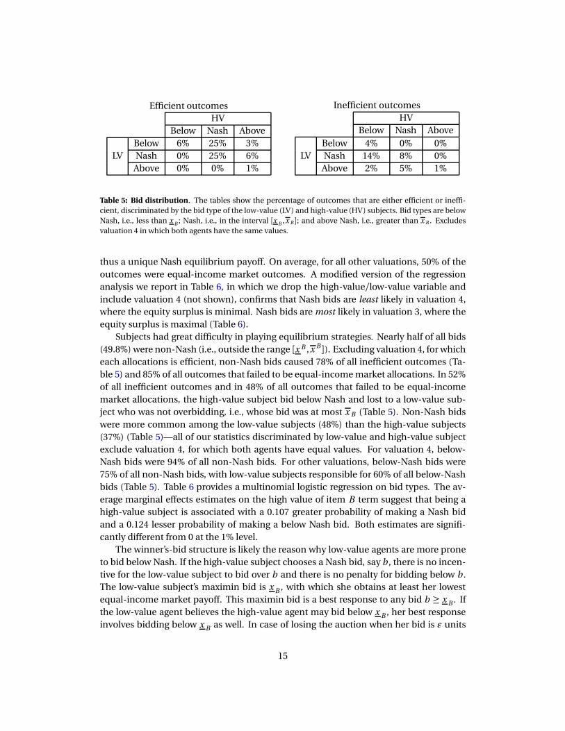
Table 5: Bid distribution. The tables show the percentage of outcomes that are either efficient or ineffi-cient, discriminated by the bid type of the low-value (LV) and high-value (HV) subjects. Bid types are belowNash, i.e., less than x B ; Nash, i.e., in the interval [x B ,x B ]; and above Nash, i.e., greater than x B . Excludesvaluation 4 in which both agents have the same values.

thus a unique Nash equilibrium payoff. On average, for all other valuations, 50% of theoutcomes were equal-income market outcomes. A modified version of the regressionanalysis we report in Table 6, in which we drop the high-value/low-value variable andinclude valuation 4 (not shown), confirms that Nash bids are least likely in valuation 4,where the equity surplus is minimal. Nash bids are most likely in valuation 3, where theequity surplus is maximal (Table 6).

Subjects had great difficulty in playing equilibrium strategies. Nearly half of all bids(49.8%) were non-Nash (i.e., outside the range [x B ,x B ]). Excluding valuation 4, for whicheach allocations is efficient, non-Nash bids caused 78% of all inefficient outcomes (Ta-ble 5) and 85% of all outcomes that failed to be equal-income market allocations. In 52%of all inefficient outcomes and in 48% of all outcomes that failed to be equal-incomemarket allocations, the high-value subject bid below Nash and lost to a low-value sub-ject who was not overbidding, i.e., whose bid was at most x B (Table 5). Non-Nash bidswere more common among the low-value subjects (48%) than the high-value subjects(37%) (Table 5)—all of our statistics discriminated by low-value and high-value subjectexclude valuation 4, for which both agents have equal values. For valuation 4, below-Nash bids were 94% of all non-Nash bids. For other valuations, below-Nash bids were75% of all non-Nash bids, with low-value subjects responsible for 60% of all below-Nashbids (Table 5). Table 6 provides a multinomial logistic regression on bid types. The av-erage marginal effects estimates on the high value of item B term suggest that being ahigh-value subject is associated with a 0.107 greater probability of making a Nash bidand a 0.124 lesser probability of making a below Nash bid. Both estimates are signifi-cantly different from 0 at the 1% level.

The winner’s-bid structure is likely the reason why low-value agents are more proneto bid below Nash. If the high-value subject chooses a Nash bid, say b , there is no incen-tive for the low-value subject to bid over b and there is no penalty for bidding below b .The low-value subject’s maximin bid is x B , with which she obtains at least her lowestequal-income market payoff. This maximin bid is a best response to any bid b ≥ x B . Ifthe low-value agent believes the high-value agent may bid below x B , her best responseinvolves bidding below x B as well. In case of losing the auction when her bid is ǫ units

15

to the left of x B , her loss, compared to her maximin payoff, is at most ǫ. If the low-valuesubject bids below Nash with some probability, the high-value subject has the incentiveto lower her bid too. The incentive is not symmetric however. The high-value subject’smaximin bid is x B , with which she obtains at least her lowest equal-income market pay-off. If the high-value subject bids below Nash and loses the auction, her worst case sce-nario loss, compared to her maximin payoff, is at least the equity surplus (see Figure 6). Ifhigh-value subjects respond to these incentives, they will be less likely to bid below Nashfor valuation structures with higher equity surplus. Regression analysis confirms this isso in our experiments (Table 6). This also explains why the auction is more efficient forvaluation structures with higher equity surplus (Figure 3). The cost of biding below Nashand losing the auction for a high-value subject increases with the efficiency surplus. Thisdiscourages high-value subjects to bid below Nash while low-value subjects retain theirincentive to hover around their lowest Nash bid. The consequence is that the percentageof efficient allocations and the percentage of equal-income market outcomes increasesas the equity surplus increases.

Below-Nash bids are a persistent phenomenon among low-value and high-value sub-jects. Figure 4 provides a breakdown of bid types averaged over the period within valu-ation. Bids above Nash levels appear to be decreasing as subjects gain more experiencewithin a valuation. If anything, subjects appear to be increasing their number of Nashbids. The regression in Table 6 is supportive of these general trends: with each succes-sive period within a valuation, subjects increase their likelihood of making a below Nashbid by 1.1 percentage points (p-value<0.05). They increase their probability of makinga Nash bid by 1.4 percentage points (p-value<0.01). They decrease their probability ofmaking an above Nash bid by 2.5 percentage points (p-value<0.01).

The persistence of below-Nash bids is a tell-tale of bounded rationality. Even if oneconsiders mixed strategies, no Nash equilibrium can sustain bids below x B − 1 for thehigh-value subject.15 In order to sustain bids below x B − 1, high-value subjects shouldnot anticipate the incentives that are induced by their behavior. Table 5 reveals the ex-tent to which below-Nash bids are not a best response for high-value subjects to thedistribution of play in our experiment. Of the high-value subjects who bid below Nash,

15No above-Nash bid can be sustained in equilibrium, for x B strictly dominates, for both high-value andlow-value subjects, a greater bid that wins with positive probability. If x B−x B > 0, the high-value subject willnever choose a below-Nash bid that loses with certainty (her expected payoff would be below her maximinpayoff). Consider now the the winner’s-bid auction in which bid ties are decided at random, assigningitem B to an agent, say i , with probability γ whenever there is a tie. In a mixed-strategy Nash equilibriumof this mechanism and in which both agents bid below Nash with positive probability, the left extreme ofthe support of each subject’s strategy has to be the same (recall that in our experiments bids are boundedbelow). This is so because no agent will choose a below-Nash bid that loses with certainty and also loses withpositive probability to some other below-Nash bid (the subject would be better off by bidding the lowest bidthat wins with positive probability, which is necessarily weakly to the left of x B ). Let b be the lowest bid ofboth agents in some mixed-strategy Nash equilibrium of the mechanism that breaks ties with probabilityγ for an agent. Then, b ≥ x B − 1, for otherwise the agent who wins ties with probability at most 1/2 wouldgain by bidding b + 1 instead of b . Thus, independently of the tie-breaker, a high-value agent would neverbid below x B −1 in a mixed-strategy equilibrium.

16

Bid type:below Nash

bida

Nashbida

above Nashbida

period within 0.011** 0.014*** -0.025***valuation (0.005) (0.005) (0.004)

has high value -0.124*** 0.107*** 0.018on item B (0.028) (0.029) (0.018)

valuation 1b 0.120*** -0.187*** 0.074**(40-80) (0.043) (0.046) (0.033)

valuation 2 0.228*** -0.120** -0.108***(120-160) (0.046) (0.047) (0.027)

valuation 3 -0.160*** 0.257*** -0.097(40-120) (0.037) (0.044) (0.026)

Type of regression? multinomial logistic

Dummy variables?b each valuation (shown above)

First random effects term? subject

Second random effects term? none

observationsc 304 554 102log likelihood -884.377

* Significant at the 10% level.** Significant at the 5% level.*** Significant at the 1% level.

a. Average marginal effects reported.b. Valuation 5 dummy variable is omitted.c. There are 960 total observations used in the regression.

Table 6: Regression of bid type for winner’s-bid auction on valuation, period within valuation, and sub-

ject’s value on item B , controlling for subject random effects. (Valuation 4, for which there is no well-defined high-value/low-value subjects, is excluded).

24% win the auction and 16% lose to a below Nash bid. This reflects that low-value sub-jects have lower cost of underbidding and end up doing it with higher probability. Thisis not enough to make bidding below Nash a rational choice for a high-value agent. Ofthe high-value subjects who bid below Nash, 53% lose to a Nash bid. The average Nashbid by the low-value subjects is closer to x B than x B .16 The result is that a high-valuesubject who underbids in our experiment would be better off, on average, by attemptingto capture half of the equity surplus. Indeed, high-value subjects’ average profit wouldincrease by 3.5% if, ceteris paribus, their below-Nash bids were replaced by (x B +x B )/2.Since high-value subjects are underbidding, low-value subject’s best response to high-value subject’s distribution of play involves underbidding. Low-value subjects that un-derbid in our experiment do it more aggressively than it is optimal, however. Of the low-value subjects who bid below Nash, 16% lose to a below-Nash bid and 11% win against abelow-Nash bid; low-value subjects’ average profit would increase by 0.15% if all below-

16On average, low-value players with Nash bids, attempt to obtain 38% of the equity surplus, i.e., bid onaverage x B +0.38(x B −x B ).

17

b

b

b bb

b

b b0

0.1

0.2

0.3

0.4

0.5

0.6

0.7

0.8

0.9

1.0

1 2 3 4 5 6 7 8 9 10

Period within valuation

Shar

e

Nash bids

below-Nash bids

Low-value subject

b

b

b bb

b

b b0

0.1

0.2

0.3

0.4

0.5

0.6

0.7

0.8

0.9

1.0

1 2 3 4 5 6 7 8 9 10

Period within valuation

Shar

e

Nash bids

below-Nash bids

High-value subject

Figure 4: Share of bid types in the winner’s-bid auction over period within valuation by subject value onitem B . Valuation 4 excluded.

Nash bids were replaced by x B and by 1.1% if all below-Nash bids were replaced by x B−9(low-value subjects’ average profit would decrease if below-Nash bids were replaced bya bid below x B − 9).

It is worth noting that the prevalence of below Nash bids is consistent with a QuantalResponse Equilibrium (QRE) model (McKelvey and Palfrey, 1995). QRE has been suc-cessful in describing subjects play distribution in a wide range of simultaneous movegames (Goeree et al., 2005). It assumes that subjects noisily best respond with a distri-bution that is monotone with respect to the agent’s utility. In our winner’s-bid auction,this monotonicity implies that the low-value agent is more prone to underbid, for con-ditional on losing the auction, she has no penalty for lowering her bid. This is a plausibleexplanation that sustains the actual distributions of play. Since the main purpose of thispaper is to compare the winner’s-bid auction with the divide-and-choose mechanism,we do not pursue the fit of our data to the QRE hypothesis. We do so in the companionpaper, Brown and Velez (2015), in which we test the comparative statics that QRE behav-ior predicts for winner’s-bid auction and competing simultaneous-move mechanisms—more on this in Sec. 5.

Result 3. The failure to achieve equal-income market and efficient outcomes in the divide-

and-choose is primarily due to the second-mover choosing against self-interest and effi-

ciency, rather than the divider’s failure to make equal-income market divisions. Nearly all

of these suboptimal choices occur when the chooser receives less than one-third of the eq-

uity surplus. Consistent with inequality aversion, the chooser is far more likely to choose

against self-interest and efficiency when holding the low value on item B.

With the divide-and-choose mechanism, there were 133 (of 700, see Table 3) out-comes that were not equal-income market outcomes. Of these, 45 involved the divider

18

proposing a non-equal-income market division, meaning that independently of the choiceof the second-mover, the outcome would not be an equal-income market outcome. Inthe remaining 88 cases, the divider proposed a division that would have been an equal-income market outcome provided the chooser selects the option in line with her self-interest.17 Instead, the chooser chose the least preferred bundle (i.e., item and transferpayment). We refer to these situations in which the chooser chose against self-interest as“rejections.” Interestingly, while the tendency of dividers to propose non-equal-incomemarket divisions abates with experience, the tendency of choosers to reject market pro-posals persists. Only 7 of the 45 (15.6%) non-equal-income market divisions occur aftermore than 5 periods of experience within a valuation, but 45 of the 88 (51.1%) of thechoices against self-interest do. Regression results, using valuation fixed effects and theperiod within valuation variable (not shown) suggest non-equal-income market propos-als and choices against self interest reduce by 34% (p < 0.01) and 4% (p ≈ 0.388), respec-tively, each successive period within a valuation.

The choices by the second mover against self-interest are hardly random (Fig. 5).They occur most frequently when the divider’s proposal is close to the sub-game perfectprediction. Moreover, among the proposals that are close to sub-game perfect propos-als, those made by the high-value subject are rejected with higher probability than thosemade by the low-value subject. To more carefully analyze this behavior, we classify eachequal-income market division by whether the chooser receives less than a third of theequity surplus (divider-favored divisions), between one-third and two-thirds of the eq-uity surplus (even divisions), and over two-thirds of the equity surplus should she choosethe option consistent with self-interest and efficiency (chooser-favored divisions)—thisis equivalent to dividing the interval [x B ,x B ] in three subintervals of equal size. The re-sults are striking: the chooser chose against self-interest in 26.6% (87 of 327) of dividerfavored divisions, in 0.4% (1 out of 225) of the even divisions, and in 0% (0 of 103) of thechooser-favored divisions (Figure 5).

A first observation is that in a proposal that is close to the sub-game perfect one,there is little payoff difference between the second mover’s choices (Fig. 6 (a)). Indeed,the “rejection cost,” i.e., the difference in payoff between the two options for the chooser,is zero for a sub-game perfect proposal and increases linearly as the proposal movesaway from this sub-game perfect prediction (Fig. 6 (b)). For the 88 choices against self-interest of equal-income market divisions, the average difference between the two op-tions for the chooser was 4.35 experimental units. For the 567 choices consistent withself-interest of equal-income market divisions, the average difference was 15.67 exper-imental units. It is not just about personal incentives, however. With the divide-and-choose mechanism, low incentives for the chooser to choose self interest are also tiedwith reciprocity motivations. If the rejection cost for a chooser is r , the divider wouldlose the efficiency surplus minus r in case of rejection. Thus, a small difference betweentwo options for the chooser means the divider has proposed to capture much of the ef-

17In only one case did the divider propose a non-equal-income market division and the chooser choseagainst self-interest. That case is only counted as one of the 45 non-equal-income market divisions.

19

equal-income market allocations

| | | |

x Bx B

(x B +x B )/3

Divider

Rejected

Accepted

HV LV

||

||

20%

40%

60%

80%

t B

Figure 5: Distribution of equal-income market proposals from high-value (HV) and low-value (LV) sub-

jects in divide-and-choose mechanism. Horizontal axis shows t B , the transfer from the agent who receivesitem B to the other agent. Excludes valuation 4, i.e., (160, 160). Low-value subject’s proposals are closerto sub-game perfect Nash proposals than high-value subject’s proposals. Proposals made by the low-valuesubject that are closer to sub-game perfect Nash proposals are rejected with lower probability than thosemade by the high-value subject. Rejection means the chooser chooses the inefficient allocation that doesnot increase her payoff and induces a loss for the divider. Compare to the theoretical predictions of thedivide-and-choose mechanism in Fig. 1.

ficiency surplus. For example, in valuations 1, 2 and 5, a difference of 4.35 experimentunits between the efficient option and the non-efficient option for the chooser meansthe divider will get 35.65 experiment units more, should the chooser pick her preferredoption.18

Rejection incentives are not symmetric for low-value and high-value subjects. Fig-ure 6 (b) shows the effect in the difference in final payoffs that is induced by a rejectiondecision. This change is independent of who is making the rejection decision. On theone hand, if the left extreme proposal, i.e., x B , is accepted, the difference in payoffs is theefficiency surplus. If this proposal is rejected, there is equality of payoffs. Thus, rejectionof such a proposal decreases inequality of payoffs by an amount equal to the efficiencysurplus. This means that the rejection by a low value subject of a sub-game perfect pro-posal reduces inequality of payoffs. On the other hand if the right extreme proposal, i.e.,x B , is accepted, the difference in payoffs is zero. If this proposal is rejected, the differ-ence in payoffs is the efficiency surplus. Thus, rejection of such a proposal increasesinequality of payoffs by an amount equal to the efficiency surplus. This means that therejection by a high-value subject of a sub-game perfect proposal increases inequality ofpayoffs. Our data largely supports that agents take into consideration the inequality ofpayoffs consequences of their rejection decisions: of the sub-game-perfect divisions, thechooser chooses against efficiency 59.0% of the time (13 of 22) with the low value andonly 33.3% (18 of 54) with the high value. With divider-favored divisions (i.e., those at

18In valuation 3, the efficiency surplus is 80, meaning such a proposal would give the divider 75.65 shouldthe chooser follow her self interest. In valuation 4, all outcomes are efficient so the only equal-incomemarket division gives equal earnings to each agent.

20

x Bx B

HV payoff efficient outcome

LV payoff efficient outcome

HV payoff inefficient outcome

LV payoff inefficient outcome

HV

reje

ctio

nco

st

LVre

ject

ion

cost

Effi

cien

cysu

rplu

s

(a)

x Bx B

chan

gein

diff

eren

cein

payo

ffs

indu

ced

byre

ject

ion

HV rejection cost

LV rejection cost

(b)

Effi

cien

cysu

rplu

s

Figure 6: Incentives in divide-and-choose. (a) Subjects payoffs from divisions in the range [x B ,xB]. For

a given proposal x ∈ [x B ,x B], the payoff of the high value subject in case the proposal is accepted, i.e.,

the chooser choses the efficient outcome, is given by the line labeled “HV payoff efficient outcome.” Theother lines represent the respectively labeled payoffs. (b) A subject’s rejection cost is given by the differencebetween her payoff if the efficient outcome is chosen and her payoff if the inefficient outcome is chosen(solid lines). The gray dashed line shows the change in difference in payoffs that is induced by rejecting aproposal. For instance, rejecting proposal x B generates equal payoffs. Accepting this proposal generatespayoffs that differ by the efficiency surplus. Thus, rejecting proposal x B reduces the difference in payoffs bythe efficiency surplus.

which the chooser receives up to one third of the efficiency surplus), she chooses againstefficiency 37.8% of the time (56 of 148) with the low value and only 17.3% (31 of 179) withthe high value.

Table 7 provides regression analysis of the propensity for dividers to choose againstself interest using our classification of proposals in three regions of equal lenght (divider-favored, neutral, chooser-favored), the cost in making this choice, and the difference ininequality induced by rejection. The analysis confirms the general trends noted earlier.Every additional experimental earning point lost when choosing against self interest re-duces the probability of choosers choosing against self interest by 1.8 percentage points.For every additional one point difference in the magnitude of inequality of earnings thatcan be eliminated by choosing against self interest, choosers increase their probabilityof choosing against self-interest by 0.2 percentage points. It is also interesting to notethe terms not found to be significant in the regression. The sign on the “period withinvaluation” term is not significantly different than 0, suggesting these type of decisions bythe chooser do not depend on experience. Further, the “divider-favored proposal term”is also not significantly different than 0. As these type of proposals are the type that aremost favorable to the divider, it is reasonable to expect they should generate the mostnegative reciprocity from the chooser. As these proposals do not produce a differential

21

Dependent variable: Choice against self interesta

period within valuation -0.001(0.004)

difference in individual payoffs -0.018***between choices (0.003)

difference in inequality -0.002***between choices (0.000)

divider-favored proposal 0.038(0.075)

Type of regression? logistic

Fixed effects? each valuation (shown above)

First random effects term? second-mover (chooser)

Second random effects term? none

observations 522b

log likelihood -132.286

* Significant at the 10% level.** Significant at the 5% level.*** Significant at the 1% level.

a. Average marginal effects reported. A similar table showing logit coefficients is provided in our supple-mental materials.b. Results are restricted to equal-income market proposals that are not in valuation 4 or chooser-favoreddivisions. As choices are equal for equal-income market proposals in valuation 4, there is no way a choosercould choose against self-interest or efficiency. No chooser chose against self-interest with a chooser-favored division, so estimating its logistic term is problematic.

Table 7: Regressions of chooser choice against self-interest (and efficiency) with equal-income market

divisions in divide-and-choose mechanism, controlling for subject random effects.

reaction from the chooser, we may speculate that these reciprocal motives are less im-portant in the divide-and-choose mechanism.

Result 4. There is no evidence of the theoretically-predicted first-mover bias in the divide-

and-choose mechanism.

Sub-game perfect equilibrium predicts that the divide-and-choose mechanism fa-vors the divider. In our experimental environment, this is not the case. Table 8 pro-vides the results from six regressions of subject profit and share of combined profit withdummy variables for first mover and high value on item B . The regressions use similarfixed and random effects as before (see equations (1) and (2)). The first two regressionsindicate a second-mover advantage in divide-and-choose. Dividers receive on averageabout 4.5 points (2.5%) less (p<0.01) than choosers (see row 2, columns 1 and 2).

Result 3 provides some explanation as to why there is no first-mover advantage inthe divide-and-choose mechanism. First-movers do not often propose to capture all thesurplus; when they propose to capture more than two-thirds of the surplus, chooserschoose against their self-interest and efficiency about 26.6% of the time. Table 8 alsoprovides regressions on “proposed allocations,” i.e., how allocations would be decided

22

if the second-mover never rejected a proposal. Recall that for divide-and-choose weconsider a “rejection” to be any time the chooser chose an option that provided the lower

payoff for both players.19 As expected, these results (Table 8, columns 3 and 4) favor thefirst mover more. First movers propose to take about 1.5 points (1% share) more than thesecond mover, a significant difference (p < 0.05 and p < 0.01, respectively).20

The last two columns of Table 8 (columns 5 and 6) show regressions on subject earn-ings restricted to proposals that are not rejected. The first-mover advantage falls be-tween the values for overall results (columns 1 and 2) and proposed allocations (columns3 and 4). Not surprisingly, this indicates that proposals that favor the second-movermore are more likely to be accepted. Also, the act of rejection reduces the discrepancybetween the first and second mover’s earnings. These rejections cause an outcome withhigher earnings for the second player, enough to erode any first-mover advantage.

One can relate the absence of first-mover advantage in our experimental results andthe chooser’s advantage predicted for divide-and-choose under incomplete informationwhen agents are risk averse (McAfee, 1992; Kittsteiner et al., 2012). With incomplete in-formation a divider is uncertain of the the other agent’s valuations. The consequenceis that her equilibrium proposal, which best responds to her prior on the other agent’swillingness to pay for the good, may induce inefficient allocations with positive prob-ability (McAfee, 1992).21 Similarly, a divider in our experiments has uncertainty aboutwhat proposals will be “accepted” by the chooser. In both cases, the divider bears all riskin the allocation process and absorbs a disproportionate share of the efficiency loss.

Result 5. The efficiency gains from using the divide-and-choose mechanism instead of

the winner’s-bid auction are primarily realized by low-value subjects and second-movers

in the divide-and-choose. Profits for high-value first-movers are not significantly different

under either mechanism.

The additional surplus generated by the divide-and-choose mechanism comparedwith the winner’s-bid auction (Result 1) is not distributed equally among the differentroles in this mechanism. Our regression analysis (Table 8) allows us to conclude that theprofit difference between high-value and low-value subjects in the winner’s-bid auctionis greater than in the divide-and-choose (23.052 vs 19.560, total points, p < 0.05; 14.438%vs. 10.186%, percent share, p < 0.01). Since the divide-and-choose mechanism favorsthe second mover (Result 4), low-value choosers would benefit the most and high-valuedividers would benefit the least from using the divide-and-choose mechanism insteadof the winner’s-bid auction.

19In the case of equal payoffs, a rejection is when the second player would choose inefficiency (and givingthe first mover less) over efficiency (and giving the first mover more).

20If we restrict these regressions to only equal-income market proposals (not shown), first movers take6.27 points (4%) more in their proposals (p<0.01), suggesting off-equilibrium play is responsible for someof the reduction in the first-mover advantage with divide-and-choose.

21Efficiency of the divide-and-choose mechanism is recovered if the role of the divider is assigned in anascending price auction (de Frutos and Kittsteiner, 2008).

23

conditon: overall proposed offersa accepted offersa

dependent profit share of profit share of profit share ofvariable: (in total profit (in total profit (in total profit

points) (percent)a points) (percent)a points) (percent)a

(1) (2) (3) (4) (5) (6)

Divider/first mover in -4.481*** -2.560*** 1.663** 1.184*** -0.950 -0.273divide-and-choose (1.200) (0.694) (0.811) (0.475) (0.875) (0.508)

High value on B in 19.560*** 10.582*** 19.745*** 10.186*** 18.388*** 9.248***divide-and-choose (1.20) (0.696) (0.811) (0.461) (0.857) (0.498)

High value on B in 23.052*** 14.438*** - - - -winner’s-bid auction (1.298) (0.526)

Winner’s-bid auction -7.195*** -3.200*** - - - -(1.968) (1.222)

Type of regression? linear linear linear linear linear linear

Fixed effects? each period each period each period each period each period each period

First random subject subject subject who is subject who is subject subjecteffects term? first mover first mover

Second random player paired player paired none none player paired player pairedeffects term? with subject with subject with subject with subject

observations 2080 2080 1120 1120 942 942log likelihood -9193.165 -8057.151 -4507.566 -3875.03 -3777.262 -3263.333

* Significant at the 10% level.** Significant at the 5% level.*** Significant at the 1% level.

a. In divide-and-choose, a rejection is the divider choosing the option that gives him less points, or in a case of equal points, the inefficient outcome. Thus adivider’s proposal is what would be implemented given the chooser does not reject. Auction data are not included for these four regressions.

Table 8: Regressions of subject earnings on mechanism, valuation, first mover, and item B value, controlling for period fixed effects and subject random

effects. Valuation 4 is excluded from analysis.

24

value type: low high

divider2.714

(1.987)-0.778(1.968)

chooser7.195***(1.968)

3.703*(1.987)

1/2 divider + 1/2 chooser4.954***(1.884)

1.463(1.884)

* Significant at the 10% level.** Significant at the 5% level.*** Significant at the 1% level.

Table 9: Average payoff in divide-and-choose mechanism minus average payoff in winner’s-bid auction.

Results are linear combinations of the coefficients found in regression (1) in Table 8.

Table 9 interprets the coefficients from regression (1) in Table 8 to show the gainor loss from moving from the divide-and-choose mechanism to the winner’s-bid auc-tion by role and valuation type. We can conclude that a chooser is better off using thedivide-and-choose mechanism than the winner’s-bid auction, especially if she held thelow value on item B . A divider in the divide-and-choose does slightly better than thewinner’s-bid auction if she holds the low value. By contrast, a divider in the divide-and-choose does slightly worse than the winner’s-bid auction if she holds the high value.However, neither result is statistically significant. Since the decision to use these mech-anisms may be made independent of knowing the role in the divide-and-choose for ei-ther player, we also include this comparison in the case where there is a random (50/50)chance of being a divider or chooser.22 In this case the net earnings gain form usingthe divide-and-choose is positive for high-value and low-value subjects, but only signif-icantly different from zero in the low-value case.

5 Discussion and concluding remarks

We have presented evidence that the divide-and-choose mechanism is superior to thewinner’s-bid auction in an experimental environment in which agents know each other’spayoffs. Our understanding of the reasons why behavior in both mechanisms deviatesfrom theoretical predictions points to clear directions in which they can be improved.

First, our results show that agents reject proposals that are perceived as biased to-wards the divider in the divide-and-choose mechanism. These proposals are less likelyto be rejected when they induce equality instead of inequality of payoffs. Thus, it is plau-sible that a mechanism that selects in sub-game perfect equilibria an allocation that is

22One should think of our results as providing evidence for agents who write a partnership contract be-hind the veil of ignorance. If subjects, after values are realized, choose the mechanism to be used in theallocation process, they may favor inefficient options (Brooks et al., 2010).

25

a better compromise in the set of equal-income market allocations may attain a betterperformance than divide-and-choose in terms of our two criteria of efficiency and eq-uity. Based on this intuition Nicolò and Velez (2014) have designed an offer-counter-offermechanism, which allows agents to compromise in a more balanced market allocationwhich does not depend on who is selected as first mover.

Second, since the winner’s-bid auction is substantially affected by the effect that si-multaneous play has on bounded rationality of subjects, it is plausible that the sameeffect is extended to other simultaneous move mechanisms that implement in Nashequilibria equal-income market allocations. Relevant alternatives include the so calledα-auctions (Cramton et al., 1987) and the direct revelation mechanism that selects theequal-income market allocation whose transfer is closest to zero (Abdulkadiroglu et al.,2004).23 The α-auctions, where α ∈ [0,1], operate as follows. Ask both agents to reportbids for the item; then, an agent with the highest bid receives the item and transfersthe other agent the α convex combination between the highest and the lowest bid.24

In an independent private-value setting, all α-auctions are ex-post-efficient, interim-individually-rational, and incentive-compatible for a non-trivial set of ownership distri-butions that contains and is centered in the symmetric ownership case (Cramton et al.,1987). When information is complete, each α-auction is strategically equivalent to adirect mechanism that selects an equal-income market allocation for the reported pref-erences. The equilibria of all these mechanisms for a given preference profile is exactlythe set of all equal-income market allocations for the true preferences (Tadenuma andThomson, 1995a) —notice that the mechanism proposed by Abdulkadiroglu et al. (2004)also belongs to this family.25 It is plausible that the QRE model (McKelvey and Pal-frey, 1995), which is consistent with the distribution of play in our experiments with thewinner’s-bid auction, is also consistent with the distribution of play in these alternativesimultaneous-move mechanisms. Thus, our results point to a behavioral model that canbe used to discriminate among otherwise equivalent options. This, which is beyond thescope of this paper, is investigated by Brown and Velez (2015).

References

Abdulkadiroglu, A., Sönmez, T., Ünver, M. U., 06 2004. Room assignment-rent division:A market approach. Soc Choice Welfare 22 (3), 515–538.

Andreoni, J., Che, Y.-K., Kim, J., 2007. Asymmetric information about rivals’ types in stan-dard auctions: An experiment. Games Econ Behavior 59 (2), 240 – 259.

23The mechanism proposed by Abdulkadiroglu et al. (2004) can be framed as an auction in which bids areinterpreted as half values. This mechanism is used by Spliddit (2014).

24Fair Outcomes Inc. (2007-2013) uses the average price auction, i.e., the 1/2-auction.25The result in (Tadenuma and Thomson, 1995a) applies only to the single-good or two-agent case. This

result has been generalized to the n-agent and n-item case (Beviá, 2010; Azacis, 2008; Velez, 2011).

26

Azacis, H., 2008. Double implementation in a market for indivisible goods with a priceconstraint. Games Econ Behavior 62, 140–154.

Beviá, C., 2010. Manipulation games in economies with indivisible goods. InternationalJournal of Game Theory 39 (1), 209–222.

Brooks, R. R. W., Landeo, C. M., Spier, K. E., 2010. Trigger happy or gun shy? dissolvingcommon-value partnerships with Texas shootouts. RAND J Econ 41 (4), 649–673.

Brown, A. L., Velez, R. A., 2015. Optimal α-auctions, Mimeo, Texas A&M University.

Charness, G., Rabin, M., 2002. Understanding social preferences with simple tests. Quar-terly journal of Economics, 817–869.

Che, Y.-K., Hendershott, T., June 2008. How to divide the possession of a football? EconLetters 99 (3), 561–565.

Cooper, D. J., Fang, H., 2008. Understanding overbidding in second price auctions: Anexperimental study. The Economic Journal 118 (532), 1572–1595.

Costa-Gomes, M. A., Weizsäcker, G., 2008. Stated beliefs and play in normal-form games.The Review of Economic Studies 75 (3), 729–762.

Cramton, P., Gibbons, R., Klemperer, P., 1987. Dissolving a partnership efficiently. Econo-metrica 55 (3), pp. 615–632.

de Frutos, M.-A., Kittsteiner, T., 2008. Efficient partnership dissolution under buy-sellclauses. The RAND Journal of Economics 39 (1), 184–198.

Dupuis-Roy, N., Gosselin, F., 2009. An empirical evaluation of fair-division algorithms.In: Love, B. C., McRae, K., Sloutsky, V. M. (Eds.), Proceedings of the 30th Annual Con-ference of the Cognitive Science Society. Cognitive Science Society, Amsterdam, NL,pp. 2681–2686.

Dupuis-Roy, N., Gosselin, F., 2011. The simpler, the better: a new challenge for fair-division theory. In: Love, B. C., McRae, K., Sloutsky, V. M. (Eds.), Proceedings of the32th Annual Conference of the Cognitive Science Society. Cognitive Science Society,Amsterdam, NL, pp. 3229–3234.

Fair Outcomes Inc., 2007-2013. Fair buy-sell.URL http://www.fairoutcomes.com/fb.html

Fischbacher, U., 2007. Z-tree: Zurich toolbox for ready-made economic experiments.Experimental Economics 10 (2), 171–178.

Foley, D., 1967. Resource allocation and the public sector. Yale Economic Essays 7, 45–98.

27

Goeree, J. K., Holt, C. A., Palfrey, T. R., 2005. Regular quantal response equilibrium. Ex-perimental Economics 8 (4), 347–367.URL http://dx.doi.org/10.1007/s10683-005-5374-7

Greiner, B., 2004. The online recruitment system orsee 2.0 — a guide for the or-ganization of experiments in economics. University of Cologne Discussion Paper(www.orsee.org).

Guth, W., Schmittberger, R., Schwarze, B., 1982. An experimental analysis of ultimatumbargaining. Journal of Economic Behavior & Organization 3 (4), 367 – 388.

Herreiner, D. K., Puppe, C. D., 2009. Envy freeness in experimental fair division problems.Theory and Decision 67, 65–100.

John, O. P., Naumann, L. P., Soto, C. J., 2008. Paradigm shift to the integrative big-five traittaxonomy: History, measurement, and conceptual issues. In: John, O. P., Robins, R. W.,Pervin, L. A. (Eds.), Handbook of Personality: Theory and Research. Guilford Press,New York, NY, pp. 114–158.

Kittsteiner, T., Ockenfels, A., Trhal, N., 2012. Partnership dissolution mechanisms in thelaboratory. Econ Letters 117 (2), 394 – 396.

McAfee, P. R., 1992. Amicable divorce: Dissolving a partnership with simple mechanisms.Journal of Economic Theory 56 (2), 266–293.

McKelvey, R. D., Palfrey, T. R., 1995. Quantal response equilibria for normal form games.Games and Economic Behavior 10 (1), 6–38.

Moulin, H., 2006. Social choice. In: Weingast, B. R., Wittman, D. A. (Eds.), Handbook ofPolitical Economy. Oxford University Press, pp. 373–389.

Nicolò, A., Velez, R., 2014. Divide and compromise, Mimeo.

Radner, R., 1980. Collusive behavior in noncooperative epsilon-equilibria of oligopolieswith long but finite lives. J Econ Theory 22 (2), 136 – 154.

Roider, A., Schmitz, P. W., 2012. Auctions with anticipated emotions: Overbidding,underbidding, and optimal reserve prices. The Scandinavian Journal of Economics114 (3), 808–830.

Schneider, G., Krämer, U. S., 2004. The limitations of fair division: An experimental eval-uation of three procedures. Journal of Conflict Resolution 48 (4), 506–524.

Spliddit, 2014.URL http://www.spliddit.org/

Splitwise Inc., 2014. Split expenses with friends: Splitwise.URL http://splitwise.com

28

Svensson, L.-G., 1983. Large indivisibles: an analysis with respect to price equilibriumand fairness. Econometrica 51, 939–954.

Tadenuma, K., Thomson, W., May 1995a. Games of fair division. Games and EconomicBehavior 9 (2), 191–204.

Tadenuma, K., Thomson, W., 1995b. Refinements of the no-envy solution in economieswith indivisible goods. Theory and Decision 39, 189–206.

Thomson, W., 2010. Fair allocation rules. In: Arrow, K., Sen, A., Suzumura, K. (Eds.),Handbook of Social Choice and Welfare. Vol. 2. North-Holland, Amsterdam, New York,Ch. 21.

Varian, H. R., 1976. Two problems in the theory of fairness 5 (3-4), 249–260.

Velez, R. A., 2011. Are incentives against economic justice? J Econ Theory 146, 326–345.

Velez, R. A., 2015. Sincere and sophisticated players in an equal-income market. J EconTheory 157 (0), 1114–1129.

29