Staff Working Paper ERSD-2019-10 8 November 2019 ______________________________________________________________________

World Trade Organization

Economic Research and Statistics Division

______________________________________________________________________

The WTO Global Trade Model:

Technical documentation

Angel Aguiar Erwin Corong

Dominique van der Mensbrugghe Center for Global Trade Analysis (GTAP), Purdue University

Eddy Bekkers Robert Koopman

Robert Teh World Trade Organization (WTO)

Manuscript date: 6 November 2019

______________________________________________________________________________ Disclaimer: This is a working paper, and hence it represents research in progress. This paper represents the opinions of individual staff members or visiting scholars and is the product of

professional research. It is not meant to represent the position or opinions of the WTO or its Members, nor the official position of any staff members. Any errors are the fault of the author.

The WTO Global Trade Model: Technical documentation

by

Angel Aguiar, Erwin Corong, Dominique van der Mensbrugghe, Eddy Bekkers, Robert Koopman and Robert Teh

6 November 2019

Abstract This document provides a technical description of the WTO Global Trade Model developed by the Center for Global Trade Analysis (GTAP) and the World Trade Organization (WTO). The model can be used to generate global trade projections and to assess the medium and long run effects of a wide range of global and national trade policies. The WTO Global Trade Model is a recursive dynamic extension of the static GTAP model (Corong et al., 2017), and implements a parsimonious approach to incorporate monopolistic competition—i.e., Eithier-Krugman or Melitz-type firm heterogeneity— in the standard GTAP model following Bekkers and Francois (2018). Keywords: Computable general equilibrium; recursive dynamics; baseline projections;

international trade JEL-codes: C68, F12, F17

The WTO Global Trade Model: Technical documentation

Angel AguiarErwin Corong

Dominique van der MensbruggheCenter for Global Trade Analysis (GTAP), Purdue University

Eddy BekkersRobert Koopman

Robert TehWorld Trade Organization (WTO)

November 6, 2019

Abstract

This document provides a technical description of the WTO Global Trade Model developed by theCenter for Global Trade Analysis (GTAP) and the World Trade Oranization (WTO). The model canbe used to generate global trade projections and to assess the medium and long run effects of a widerange of global and national trade policies. The WTO Global Trade Model is a recursive dynamicextension of the static GTAP model (Corong et al., 2017), and implements a parsimonious approachto incorporate monopolistic competition—i.e., Eithier-Krugman or Melitz-type firm heterogeneity—in the standard GTAP model following Bekkers and Francois (2018).

Contents

1 Introduction and overview 1

2 Core model 32.1 Overview . . . . . . . . . . . . . . . . . . . . . . . . . . . . . . . . . . . . . . . . . . 32.2 Demand . . . . . . . . . . . . . . . . . . . . . . . . . . . . . . . . . . . . . . . . . . . 42.3 Production . . . . . . . . . . . . . . . . . . . . . . . . . . . . . . . . . . . . . . . . . 52.4 Factor supply . . . . . . . . . . . . . . . . . . . . . . . . . . . . . . . . . . . . . . . . 62.5 Trade . . . . . . . . . . . . . . . . . . . . . . . . . . . . . . . . . . . . . . . . . . . . 72.6 Savings and investment . . . . . . . . . . . . . . . . . . . . . . . . . . . . . . . . . . 9

2.6.1 Investment preliminaries . . . . . . . . . . . . . . . . . . . . . . . . . . . . . . 92.6.2 Rate-of-return sensitive investment allocation . . . . . . . . . . . . . . . . . . 92.6.3 Investment allocation based on initial capital shares . . . . . . . . . . . . . . 102.6.4 Fixed real foreign savings . . . . . . . . . . . . . . . . . . . . . . . . . . . . . 102.6.5 Fixed relative foreign savings . . . . . . . . . . . . . . . . . . . . . . . . . . . 112.6.6 Summary of investment allocation rules . . . . . . . . . . . . . . . . . . . . . 11

2.7 Income and equilibrium . . . . . . . . . . . . . . . . . . . . . . . . . . . . . . . . . . 122.8 Numéraire and closure . . . . . . . . . . . . . . . . . . . . . . . . . . . . . . . . . . . 13

2.8.1 A note on price indices . . . . . . . . . . . . . . . . . . . . . . . . . . . . . . . 132.8.2 Factor price index . . . . . . . . . . . . . . . . . . . . . . . . . . . . . . . . . 152.8.3 Price of regional Absorption and MUV price index . . . . . . . . . . . . . . . 152.8.4 Definition of GDP . . . . . . . . . . . . . . . . . . . . . . . . . . . . . . . . . 16

3 Model dynamics 193.1 Introduction . . . . . . . . . . . . . . . . . . . . . . . . . . . . . . . . . . . . . . . . . 193.2 Endowments . . . . . . . . . . . . . . . . . . . . . . . . . . . . . . . . . . . . . . . . 19

3.2.1 Population and labor force . . . . . . . . . . . . . . . . . . . . . . . . . . . . . 193.2.2 Capital . . . . . . . . . . . . . . . . . . . . . . . . . . . . . . . . . . . . . . . 203.2.3 Land and natural resources . . . . . . . . . . . . . . . . . . . . . . . . . . . . 21

3.3 Technology . . . . . . . . . . . . . . . . . . . . . . . . . . . . . . . . . . . . . . . . . 213.3.1 Multi-sector models . . . . . . . . . . . . . . . . . . . . . . . . . . . . . . . . 23

3.4 Preferences . . . . . . . . . . . . . . . . . . . . . . . . . . . . . . . . . . . . . . . . . 243.5 Policies . . . . . . . . . . . . . . . . . . . . . . . . . . . . . . . . . . . . . . . . . . . 273.6 Data sources for exogenous baseline assumptions . . . . . . . . . . . . . . . . . . . . 27

4 Conclusions and future directions 28

A Mathematical appendix 31A.1 Sets and subsets . . . . . . . . . . . . . . . . . . . . . . . . . . . . . . . . . . . . . . 31

i

List of Tables

A.1 Basic sets in the model . . . . . . . . . . . . . . . . . . . . . . . . . . . . . . . . . . . 31A.2 Commodity subsets . . . . . . . . . . . . . . . . . . . . . . . . . . . . . . . . . . . . . 32A.3 Endowment subsets . . . . . . . . . . . . . . . . . . . . . . . . . . . . . . . . . . . . . 32

ii

List of Figures

2.1 Circular flows in a regional economy . . . . . . . . . . . . . . . . . . . . . . . . . . . 42.2 Production structure . . . . . . . . . . . . . . . . . . . . . . . . . . . . . . . . . . . . 62.3 Price linkages in the model . . . . . . . . . . . . . . . . . . . . . . . . . . . . . . . . 8

iii

Chapter 1

Introduction and overview

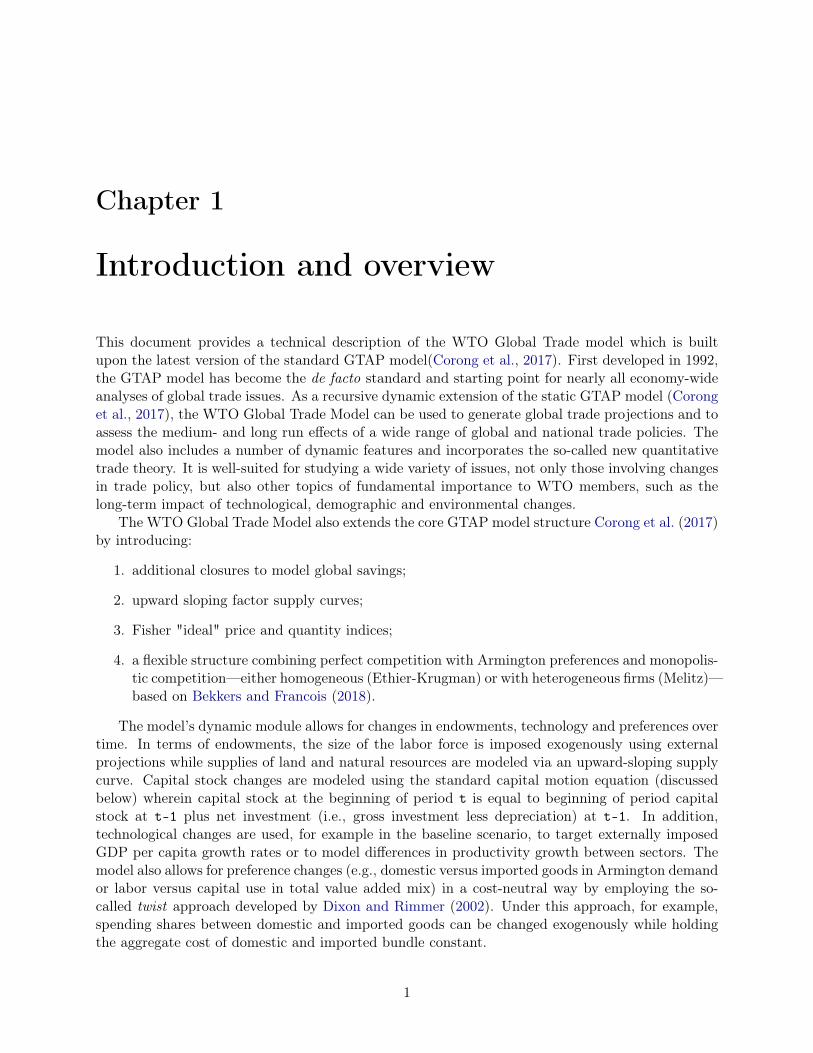
This document provides a technical description of the WTO Global Trade model which is builtupon the latest version of the standard GTAP model(Corong et al., 2017). First developed in 1992,the GTAP model has become the de facto standard and starting point for nearly all economy-wideanalyses of global trade issues. As a recursive dynamic extension of the static GTAP model (Coronget al., 2017), the WTO Global Trade Model can be used to generate global trade projections and toassess the medium- and long run effects of a wide range of global and national trade policies. Themodel also includes a number of dynamic features and incorporates the so-called new quantitativetrade theory. It is well-suited for studying a wide variety of issues, not only those involving changesin trade policy, but also other topics of fundamental importance to WTO members, such as thelong-term impact of technological, demographic and environmental changes.

The WTO Global Trade Model also extends the core GTAP model structure Corong et al. (2017)by introducing:

1. additional closures to model global savings;

2. upward sloping factor supply curves;

3. Fisher "ideal" price and quantity indices;

4. a flexible structure combining perfect competition with Armington preferences and monopolis-tic competition—either homogeneous (Ethier-Krugman) or with heterogeneous firms (Melitz)—based on Bekkers and Francois (2018).

The model’s dynamic module allows for changes in endowments, technology and preferences overtime. In terms of endowments, the size of the labor force is imposed exogenously using externalprojections while supplies of land and natural resources are modeled via an upward-sloping supplycurve. Capital stock changes are modeled using the standard capital motion equation (discussedbelow) wherein capital stock at the beginning of period t is equal to beginning of period capitalstock at t-1 plus net investment (i.e., gross investment less depreciation) at t-1. In addition,technological changes are used, for example in the baseline scenario, to target externally imposedGDP per capita growth rates or to model differences in productivity growth between sectors. Themodel also allows for preference changes (e.g., domestic versus imported goods in Armington demandor labor versus capital use in total value added mix) in a cost-neutral way by employing the so-called twist approach developed by Dixon and Rimmer (2002). Under this approach, for example,spending shares between domestic and imported goods can be changed exogenously while holdingthe aggregate cost of domestic and imported bundle constant.

1

This manual is organized as follows. The next section provides an overview of the extensionsintroduced to the core static GTAP model (Corong et al., 2017), while Section 3 provides a detaileddescription of the model’s dynamic features. Both Sections 2 and 3 include easy-to-read algebraicequations and associated TABLO codes of the model, as implemented in GEMPACK Harrison andPearson (1996). Section 4 concludes and identifies future research directions needed to improve theconstruction of dynamic baselines for the global economy and which will be the subject of a futurepaper.

2

Chapter 2

Core model

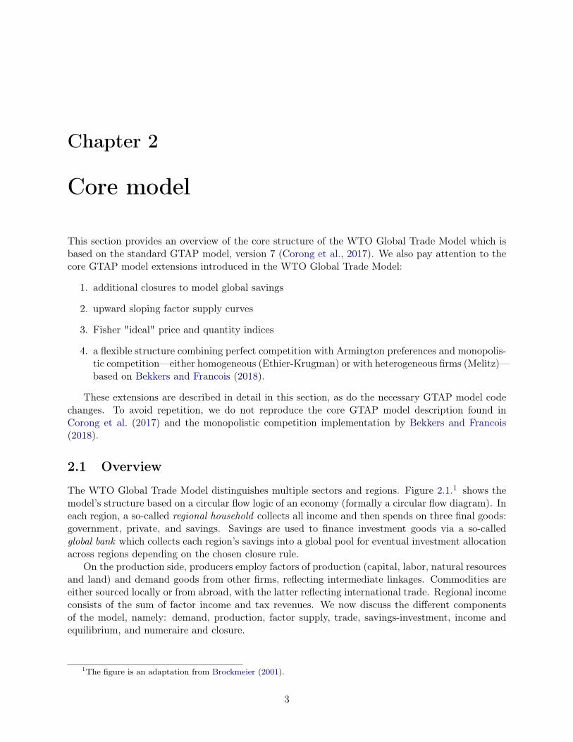
This section provides an overview of the core structure of the WTO Global Trade Model which isbased on the standard GTAP model, version 7 (Corong et al., 2017). We also pay attention to thecore GTAP model extensions introduced in the WTO Global Trade Model:

1. additional closures to model global savings

2. upward sloping factor supply curves

3. Fisher "ideal" price and quantity indices

4. a flexible structure combining perfect competition with Armington preferences and monopolis-tic competition—either homogeneous (Ethier-Krugman) or with heterogeneous firms (Melitz)—based on Bekkers and Francois (2018).

These extensions are described in detail in this section, as do the necessary GTAP model codechanges. To avoid repetition, we do not reproduce the core GTAP model description found inCorong et al. (2017) and the monopolistic competition implementation by Bekkers and Francois(2018).

2.1 Overview

The WTO Global Trade Model distinguishes multiple sectors and regions. Figure 2.1.1 shows themodel’s structure based on a circular flow logic of an economy (formally a circular flow diagram). Ineach region, a so-called regional household collects all income and then spends on three final goods:government, private, and savings. Savings are used to finance investment goods via a so-calledglobal bank which collects each region’s savings into a global pool for eventual investment allocationacross regions depending on the chosen closure rule.

On the production side, producers employ factors of production (capital, labor, natural resourcesand land) and demand goods from other firms, reflecting intermediate linkages. Commodities areeither sourced locally or from abroad, with the latter reflecting international trade. Regional incomeconsists of the sum of factor income and tax revenues. We now discuss the different componentsof the model, namely: demand, production, factor supply, trade, savings-investment, income andequilibrium, and numeraire and closure.

1The figure is an adaptation from Brockmeier (2001).

3

Rest of World

Producer

Investment

PrivateHousehold Saving Government

RegionalHousehold

XTAX MTAXVMFP VXSB

VMPP VMIP VMGP

VDPP VDGPVDIP

NETINV

PRIVEXP GOVEXPSAVE

EVOS(Endw)Taxes

Taxes

Taxes

Taxes

VDFP

Figure 2.1: Circular flows in a regional economy

2.2 Demand

For each region, a regional household allocates its income on three sources of final demand (i.e.,private, government and savings) according to a Cobb-Douglas utility function.

Expenditures on private goods are allocated across different commodities according to a non-homothetic utility, constant difference elasticity (CDE) utility function. Under non-homotheticpreferences spending shares vary with income: the share of income on food tends to fall as in-come rises, whereas the share of income spent on most service commodities tends to rise as incomeincreases. With a CDE utility function, income changes generate shifting average and marginalbudget shares. The number of parameters required by the CDE function is limited and is thus acompromise between the linear expenditure system and for example, AIDADS. The former utilityfunction is more restrictive than the CDE, as income elasticities converge quickly to one for all sec-tors, whereas the latter requires many parameters to calibrate and is not easy to reconcile correctlywith the (upper-nest) choice among government, private household and savings expenditures.

Non-homothetic preferences for private goods imply that the shares spent on the three types

4

of goods (government goods, private household goods, and savings) change with income, despitethe fact that these shares are determined by a Cobb-Douglas utility function. The share spent onprivate goods is determined by the marginal utility of private expenditures, which changes withincome. Hence, in dynamic simulations growing income will lead to changing spending shares onprivate household goods.2

Government expenditures are allocated across different commodities according to a Cobb-Douglasutility function, implying fixed commodity spending shares. Expenditures on savings are channeledto investment goods as discussed below. By including savings in the static utility function we pre-vent that a shift towards (current) consumption and away from savings (and thus implicitly fromfuture consumption) generates strong welfare effects. With savings in the static utility function wecan account for the intertemporal nature of savings-investment decisions in a static setting.3

2.3 Production

The model includes a so-called ‘make’ matrix enabling us to model either activities producing mul-tiple commodities (such as ethanol) and/or commodities produced by more than one activity (suchas electricity). On the supply side, multi-product activities produce multiple outputs according to aconstant elasticity of transformation (CET) function. On the demand side, commodities producedby various activities are combined using a CES function. The absence of multi-production impliesa diagonal make matrix–i.e., each activity produces just one commodity.

Perfectly competitive firms produce homogeneous commodities by combining value added (la-bor, capital, natural resources, and land) and intermediate inputs. The model’s nested productionstructure 2.2 assumes weak separability between value added and intermediate commodities. Thisimplies that for each activity, the price of intermediates are invariant to factor mix. The defaultallocation between intermediate and value added bundle is Leontief–hence, there is no scope for sub-stitution.4 The optimal factor mix is determined via a CES function with degree of substitutabilitygoverned by sector- and region-specific substitution elasticities (ESUBVA).

Production factors can be of three types: perfectly mobile, sluggish, or sector-specific. In thestandard closure, capital and labor are perfectly mobile, land is typically sluggish while naturalresources is sector-specific. A sluggish factor is partially mobile across sectors and is modeled ac-cording to a CET function with degree of mobility governed by elasticity of transformation ETRAE .Factor returns also vary by endowment types. Perfectly mobile factors receive uniform returns acrossactivities (i.e., an economy-wide price) while returns to sector-specific factors vary by activity. Re-turns to sluggish factors depend on their mobility (i.e., sector-specific returns if immobile or aneconomy-wide return if perfectly mobile).

2See McDougall (2003) for further discussion.3Hanoch (1975) shows formally that a static utility maximization problem with savings in the utility function is

implied by an inter-temporal consumption decision problem.4The Leontief specification can be relaxed by modifying the elasticity parameter ESUBT in the model.

5

qoa,r

CES

ESUBTa,r

qvaa,r qinta,r

CESESUBVAa,r

qfee,a,r(Nat. Res.)

qfee,a,r(Land)

qfee,a,r(Capital)

qfee,a,r(Labor)

CES

ESUBCa,r

qfac,a,r

CESESUBDc,r

qfdc,a,r qfmc,a,r

Figure 2.2: Production structure

2.4 Factor supply

The model allows for upward sloping supply specification for the non-capital endowments (land,labor and natural resources). Since upward sloping supply functions for endowments are new inthe WTO Global Trade Model, they will be discussed into detail here. A description of the setsdefinitions employed in the exposition is in Appendix A.

Equation (2.1), which is conditioned on the set ENDWMSXC 5, specifies an upward slopingsupply curve for aggregate land and labor endowments as a function of the endowment- and region-specific supply elasticity, ESUPMS e,r, and the endowment’s real return. The latter is derived as aratio of an endowment’s aggregate return, pee,r, to the private consumption price index, ppriv r.

Similarly, Equation (2.2) implements upward sloping supply for the sector-specific endowmentas a function of its supply elasticity ESUPF e,a,r and real return (i.e., sector-specific return, pese,a,r,relative to the private consumption price index, ppriv r.

qee,r = ESUPMS e,r[pee,r − ppriv r] for e ∈ {ENDWMSXC} (2.1)

qese,a,r = ESUPF e,a,r[pese,a,r − ppriv r] for e ∈ {ENDWF} (2.2)

This unit determines QE e,r for land and labor endowments, and QES e,a,r for the sector-specificendowment when the upward sloping supply specification for these factors are active. In the model

5MSXC is a shorthand for Mobile and Sluggish endowments eXcept Capital. In the model code, ENDWMSXCis derived as the complement of mobile/sluggish (ENDWMS) and capital (ENDWC ) sets.

6

code, equation E_qelsupply implements equation (2.1), while E_qesfsupply implements equa-tion (2.2).6

The TABLO codes in Listing 2.1 include two shift variables that facilitate upward sloping supplyspecification. To specify upward sloping supply for land and/or labor, the shift variable qelsupplye,rmust be swapped with qee,r in the closure file.7 Similarly, swapping the shift variable qesfsupplye,a,rwith qesf e,a,r in the closure file activates the upward sloping supply specification for the sector-specific factor.

Listing 2.1: GEMPACK equations for upward sloping supply1 Equation E_qelsupply2 # upward sloping aggregate supply specification for land (sluggish) and labor #3 (all,e,ENDWMSXC)(all,r,REG)4 qe(e,r) = ESUPMS(e,r) * [pe(e,r) − ppriv(r)] + qelsupply(e,r);

6 Equation E_qesfsupply7 # upward sloping supply specification for sector−specific (natres) factor #8 (all,e,ENDWF)(all,a,ACTS)(all,r,REG)9 qes(e,a,r) = ESUPF(e,a,r) * [pes(e,a,r) − ppriv(r)] + qesfsupply(e,a,r);

Capital supply will be discussed in Section (3).

2.5 Trade

Private, government and investment expenditures, as well as purchases of intermediate goods com-prise both domestic and imported purchases, thereby generating both domestic and export sales byfirms.

Each commodity is an aggregate of domestic and imported goods according to an ArmingtonCES specification—the so-called top-level Armington demand. The sourcing of imports by regionof origin—i.e., the second-level Armington—is done at the regional level in the destination country.This implies that goods from different regions of origins are distinct in the eyes of their buyers ordestination regions. Goods from a particular source are homogeneous: French cars are different fromGerman cars, but there is only type of French car. Because of love of variety between goods fromdifferent countries, the Armington structure allows for the possibility that each country importsgoods from each and every trading partner.

Figure 2.3 displays the price linkages in international trade. Starting from the top the figureshows activities are converted into commodities with a CET and CES. Then the figure shows thedifferent margins in international trade, in turn the export taxes, the transport margins, user-genericimport tariffs and finally user-specific import tariffs.

The international transport margin, the difference between FOB-values and CIF-values, is paidfor by using so-called margin (or transport) services supplied by the international transport sector.The quantity of transport services needed is proportional to the quantity of goods shipped. Thiscorresponds with a Leontief specification: the CIF-quantity is a Leontief aggregate of the FOB-quantity and transport services. The international transport sector in turn buys transport servicesfrom the so-called margin sectors in all countries. The three margin sectors in each exportingcountry (air transport, water transport, and other transport) sell services to the domestic market,to the exporting market and to the international transport sector

6Equations E_qelsupply and E_qesfsupply simplify to qee,r = qelsupplye,r and qese,a,r = qesfsupplye,a,r whentheir associated supply elasticities are zero.

7The user could selectively implement this specification by conditioning the swap statements with the relevantfactor sets—e.g., ENDWS if limited to the sluggish land factor, ENDWL if limited to labor, or ENDWMXSC forboth land and labor.

7

POa,rCET

‘make’

World market

PSc,a,r+TOc,a,r=PCAc,a,rCES

‘sourcing’

PDSc,r

+ + + +TFDc,a,r TPDc,r TGDc,r TIDc,r

= = = =

+TXSc,r,d

= PFDc,a,r PPDc,r PGDc,r PIDc,r

World marketPFOBc,s,d

+PTRANSc,s,d

=

PCIF c,s,d

ROW market+

TMSc,s,r = PMDSc,s,r CES‘Armington’

PMSc,r

+ + + +TFM c,a,r TPM c,r TGM c,r TIM c,r

= = = =

PFM c,a,r PPM c,r PGM c,r PIM c,r

Figure 2.3: Price linkages in the model

The WTO Global Trade Model is flexible in its trade structure, allowing to switch from thedefault perfect competition Armington specification to monopolistic competition Ethier-Krugmanor Melitz specification with respectively homogeneous or heterogeneous firms. The model followsthe setup in Bekkers and Francois (2018) making it possible to switch easily (through changes inthe parameter file) between the different trade structures. The monopolistic competition modelcombines product differentiation at the firm level (instead of the country level) with increasingreturns to scale in production: each firm (and not each country) makes a unique variety by payingfixed costs: French cars produced by different firms are perceived as separate varieties by consumers.This setup leads to so-called variety scaling of consumed goods (by private agents or firms): moreresources in a supplying country enable the country to produce more varieties and with consumersdisplaying love of variety, this leads to higher welfare and lower (welfare-adjusted) prices. Addingfirm heterogeneity to the model allows us to account for the reallocation effect of trade: moreinternational trade leads to a reallocation of market shares from less productive to more productivefirms (See Bekkers and Francois (2018) for details on modeling setup and parameterization).

8

2.6 Savings and investment

Savings in each country are collected by a global bank. The global bank spends the total amountof savings on aggregate investment goods in different countries. The aggregate investment good ineach country is a composite of investment goods.

Global savings can be allocated to investment in the different regions according to four differentforeign investment closure rules. First, global savings can be allocated to investments in differentregions such that (percentage) changes in the expected rate of return on capital are equalized acrossregions. In the second rule, investment in each country moves such that the regional compositionof capital stocks does not change. A third rule fixes net foreign capital flows in real terms. Giventhe simplified version of the balance of payments, this in essence fixes the net trade balance. Anex ante change to the trade balance, for example a tariff reduction, typically requires a change tothe real exchange rate. In this third closure option, the global bank ignores changes in the relativerates of return, as in the case of a fixed investment allocation, and it is the net saving flow thatis fixed, not the regional investment shares. A fourth mechanism fixes net capital flows relative toregional income. Both the third and fourth mechanisms can only be implemented for n− 1 regionsand thus there is a residual region that becomes the lender/borrower of last resort.

2.6.1 Investment preliminaries

Before describing the four ways to allocate global savings across investment in different regions, wedefine the nominal (after-tax) rate of return on capital and the net current rate of return on capital.

The nominal rate of return on capital, RENTALr, is defined in equation (2.3) as the product ofthe after tax return to capital in sector a, PES endwc,a,r), and the quantity of capital endowments,QES endwc,a,r, divided by the beginning-of-period capital stock, KBr:

RENTALr =∑a

PES endwc,a,rQES endwc,a,r

/KBr (2.3)

The net current rate of return on capital is equal to the nominal rate of return on capital dividedby the replacement cost of capital, PINV r, minus the deprecation rate, δr.

RORC r =RENTALrPINV r

− δr (2.4)

If a trade policy change would for example affect the price of investment goods or replacementcost of capital, then it would also affect the current rate of return on capital.

Finally, the end of period capital stock, KE r, is equal to the beginning of period capital stocknet of depreciation, (1− δr)KBr, plus new investment, QINV r:

KE r = (1− δr)KBr +QINV r (2.5)

2.6.2 Rate-of-return sensitive investment allocation

Under the first foreign investment rule the global bank responds to changes in relative rates ofreturn. According to equation (2.6) the expected rate of return, RORE r is determined by thenet rate of return, RORC r, and an additional term depending on the change in the capital stock.The expected rate of return tends to fall with a larger increase in the capital stock with elasticityRORFLEX r.

9

RORE r = RORC r

(KE r

KBr

)−RORFLEX r

(2.6)

Equation (2.6) determines the allocation of global investment funds as follows. A shock raisingthe demand for capital would increase the nominal rental rate. This in turn would lead to anincrease in the rate of return on capital, RORC r. By equation (2.6) this would raise the end-of-period capital stock, KE r, relative to beginning-of-period capital stock, KBr. The rise in KE r inturn would generate an increase in investment flows to country r. The degree to which an increasingrate of return on capital, RORC r, leads to additional investment (and thus capital inflows into acountry) is determined by RORFLEX r. A small value of RORFLEX r would generate a largerresponse in KE r and thus a larger investment response.

Under the rate-of-return sensitive investment allocation, the percentage change in the expectedrate of return in each region, RORE r, is equal to the percentage change in the global rate of return,RORG , such that the percentage change in the expected rate of return equalizes across regions.

RORE r = RORG (2.7)

2.6.3 Investment allocation based on initial capital shares

Under the second foreign investment rule the regional composition of capital stocks is invariant tovariations in changes in the expected relative rates of return. In Equation (2.8) global net investmentis defined consisting of the sum of net investment in all regions.

GLOBALCGDS =∑r

(QINV r − δrKBr) (2.8)

Under this rule regional investment is a constant share of global investment, with the sharedetermined by base investment shares, equation (2.9).

QINV r − δrKBr = χIrGLOBALCGDS (2.9)

This equation is only defined for (R − 1) regions, because the equality of global savings andglobal investment determines regional investment in the last region. Under this foreign investmentclosure the aggregate rate of return, RORG , is still defined, being equal to the weighted sum ofthe regional expected rate of return variable with the weights determined by the regional share inglobal net investment.

RORG =∑r

ϕrRORE r where ϕr =PINV r (QINV r − δrKBr)∑s

PINV s (QINV s − δsKBs)(2.10)

2.6.4 Fixed real foreign savings

We start by defining foreign savings as the difference between domestic investment and domesticsavings.

PINV rQINV r = SAVE r + FSAVE r + δrPINV rKBr (2.11)

where FSAVE r is the region’s net nominal foreign capital flow.The third specification fixes net real foreign savings—typically to base year levels, but not

required, i.e. one can shock net foreign savings. Foreign savings are fixed for n− 1 regions and are

10

given by the exogenous parameter FSAVEX , equation (2.12). These are multiplied by a global price,in this case, PGLOBALCGDS , which is the average price of investment defined in equation (2.13).Equation (2.14) is implemented to ensure that global net foreign savings sum to zero, in essenceevaluating foreign savings for the residual region.

FSAVE r = PGLOBALCGDS × FSAVEX r (2.12)

PGLOBALCGDS =∑r

PINV r (QINV r − δrKBr) (2.13)

∑r

FSAVE r ≡ 0 (2.14)

2.6.5 Fixed relative foreign savings

The fourth specification fixes net foreign savings relative to regional income. Relative foreign savingsare fixed for n − 1 regions and are set equal to the exogenous parameter χf , equation (2.15). Theparameter is calibrated to the base year ratio of foreign savings to income, but can be changed ina simulation shock. Equation (2.14) determines net foreign savings for the residual region, i.e. theborrower/lender of last resort.

FSAVE r = χfrYr (2.15)

In summary we have four foreign savings closure. Common to all closures are the following equa-tions: equation (2.5), equation (2.3), equation (2.4), equation (2.6), equation (2.8), equation (2.13),(2.11) and (2.14). Common to the last three closures, i.e. all except the rate-of-return sensitiveclosure is also equation (2.10).

2.6.6 Summary of investment allocation rules

The four cases involve specifying the following to essentially determine FSAVE :

• Rate of return sensitive investment Equation (2.7)

• Investment based on initial capital shares Equation (2.9)

• Fixed real foreign savings Equation (2.12)

• Fixed relative foreign savings Equation (2.15)

This unit determines GLOBALCGDS , KE r, RENTALr, RORC r, RORE r, QINV r and RORGusing equations E_ke, E_rental, E_rorc, E_rore, E_qinv that implements equations (2.4) and (2.9),E_globalcgds that implements equations (2.8) and (2.10), E_del_rfsave that implements FSAVEXin equation (2.12) and E_del_fsavery that implements equation (2.15).8

8The parameter RORDELTA determines global investment closure. A value of 1 uses the rate-of-return sensitiveclosure. A value of 0 uses the fixed investment allocation closure. A value of 1 coupled with the appropriate swapstatement facilitate either fixed real or fixed relative foreign savings closure. For fixed real foreign savings closure,the appropriate swap statement is: Swap cgdslack(REGN-1) = del_rfsave(REGN-1), while the appropriate swapstatement for fixed relative foreign savings closure is: Swap cgdslack(REGN-1) = del_fsavery(REGN-1). In bothcases, REGN-1 is the set of all regions except a residual region.

11

Listing 2.2: GEMPACK equations for investment allocation1 Equation E_ke2 # ending capital stock equals beginning stock plus net investment. #3 (all,r,REG)4 ke(r) = INVKERATIO(r) * qinv(r) + [1.0 − INVKERATIO(r)] * kb(r);

6 Equation E_rental7 # defines a variable for capital rental rate #8 (all,r,REG)9 rental(r) = sum{e,ENDWC, [VES(e,r) / GROSSCAP(r)] * pe(e,r)};

11 Equation E_rorc12 # current rate of return on capital in region r #13 (all,r,REG)14 rorc(r) = GRNETRATIO(r) * [rental(r) − pinv(r)];

16 Equation E_rore17 # expected rate of return depends on the current return and investment #18 (all,r,REG)19 rore(r) = rorc(r) − RORFLEX(r) * [ke(r) − kb(r)];

21 Equation E_qinv22 # either gross investment or expected rate of return in region r #23 (all,r,REG)24 RORDELTA * rore(r)25 + [1 − RORDELTA]26 * [[REGINV(r) / NETINV(r)] * qinv(r) − [VDEP(r) / NETINV(r)] * kb(r)]27 = RORDELTA * rorg + [1 − RORDELTA] * globalcgds + cgdslack(r);

29 Equation E_globalcgds30 # either expected global rate of return or global net investment #31 RORDELTA * globalcgds + [1 − RORDELTA] * rorg32 = RORDELTA33 * sum{r,REG,34 [REGINV(r) / GLOBINV] * qinv(r) − [VDEP(r) / GLOBINV] * kb(r)}35 + [1 − RORDELTA] * sum{r,REG, [NETINV(r) / GLOBINV] * rore(r)};

37 Equation E_del_rfsave38 # computes ordinary change in real foreign saving by region, $US million #39 (all,r,REG)40 del_rfsave(r) = 0.01 * [NETINV(r) * qnetinv(r) − SAVE(r) * qsave(r)];

42 Equation E_del_fsavery43 # computes change in foreign saving as a percentage of regional income #44 (all,r,REG)45 INCOME(r) * 100 * del_fsavery(r)46 = NETINV(r) * vnetinv(r) − SAVE(r) * vsave(r) − FSAVE(r) * y(r);

2.7 Income and equilibrium

The representative agent allocates income on three types of final expenditures: private, governmentand savings. Income is the sum of gross factor income and income from indirect taxes. Grossfactor income is equal to gross payments to factors of production minus depreciation. There are twotypes of indirect taxes in international transactions: Bilateral import tariffs and bilateral exporttaxes. Furthermore, there are four types of domestic taxes: sector-specific endowment taxes (firms’use of labor in the paddy rice sector); direct income tax on factor remuneration; production tax(e.g„ production of steel); and source-specific sales taxes for private, government, investment andintermediate purchases (e.g.„ tax on sales of domestic or imported raw milk to private consumers).

In equilibrium all markets clear. In particular, we impose goods market equilibrium, factor mar-ket equilibrium, transport services equilibrium, and global savings equilibrium. First, the quantity

12

produced/supplied in each country and for each commodity is equal to the domestic and exportedquantity, including margin commodities sold to the global transport sector. Second, total factorsupply equals factor demand. Third, the supply of transport services by the different margin sectorsis equal to the demand for transport services from all the bilateral trade relations. Fourth, globalsupply of savings is equal to global demand for investment. This last equation is not imposed inthe model: by Walras law one equation in the model is redundant and the difference between globalsavings and global investment (walraslack) is calculated residually to check the consistency of model.

2.8 Numéraire and closure

The default numéraire in the model is PFACTWLD, which is a weighted average of the factorprices in all regions. Before introducing this numéraire, we first turn to a discussion of the definitionor price indices.

2.8.1 A note on price indices

The model uses Fisher price indices for both factor price and GDP indices. The Fisher priceindex, sometimes also referred to as the ‘ideal’ price index (see for example Eurostat (2008)), is thegeometric mean of the Laspeyres and Paasches indices.

We outline the specification for a generic formulation before depicting the specific formulationsused in the GTAP model. For a price index over set i, the Fisher price index is equal to thefollowing:9

F p =

√ ∑i Pi,tQi,t−1∑i Pi,t−1Qi,t−1

·∑

i Pi,tQi,t∑i Pi,t−1Qi,t

=√Lp · P p

The Fisher price index represents the geometric mean of the Laspeyres (Lp) and Paasche priceindices (P p), with the former using lagged volume weights and the latter using current volumeweights.

Lp =

∑i Pi,tQi,t−1∑i Pi,t−1Qi,t−1

P p =

∑i Pi,tQi,t∑i Pi,t−1Qi,t

These indices represent percent change relative to the previous period and thus the price indicesare chain weighted. The price index itself is thus defined as:

PI t = PI t−1Fpt

where typically the price index will be set to 1 or 100 in some base period.The Fisher volume index has a similar definition using different price weights:

F q =

√ ∑i Pi,t−1Qi,t∑i Pi,t−1Qi,t−1

·∑

i Pi,tQi,t∑i Pi,tQi,t−1

=√Lq · P q

The Fisher volume index represents the geometric mean of the Laspeyres (Lq) and Paasche volumeindices (P q), with the former using lagged price weights and the latter using current price weights.

9It is natural to think of the index ‘t’ as time. However, in a comparative static framework it represents the pre-and post-shock values.

13

Lq =

∑i Pi,t−1Qi,t∑i Pi,t−1Qi,t−1

P q =

∑i Pi,tQi,t∑i Pi,tQi,t−1

It is easy to show that the aggregate nominal value is equal to the product of the price and volumeindices:

Pt ·Qt =∑i

Pi,t ·Qi,t = F pt · Fqt · Pt−1 ·Qt−1

These formulas can be log-differentiated for use in GEMPACK. We start with the followingexpressions:

Lpt =

∑iQi,t−1Pi,t∑iQi,t−1Pi,t−1

=LQ1Pt

LQ1P1tP pt =

∑iQi,tPi,t∑iQi,tPi,t−1

=LQPt

LQP1t

Since LQ1P1t only has lags, it is a constant and does not require differentiation. The other threeformulas in log-differentiated form are:

lq1pt =∑i

ϕpi,tpi,t where ϕpi,t =Qi,t−1Pi,t∑iQi,t−1Pi,t

lqpt =∑i

ϕvi,t (qi,t + pi,t) where ϕvi,t =Qi,tPi,t∑iQi,tPi,t

lqp1t =∑i

ϕqi,tqi,t where ϕqi,t =Qi,tPi,t−1∑iQi,tPi,t−1

We can insert these in the expression for Lp and P p:

lpt = lq1pt ppt = lqpt − lqp1t

The final step is to insert these expressions into the price index:

pt = 0.5[lpt + ppt ]

Thus we can proceed in four steps:

1. Calculate the share vectors, of which there are three: ϕp, ϕv and ϕq

2. Calculate the percentage change in the numerators and denominators of the Laspeyres andPaasche indices—using the weights

3. Calculate the percentage change in the Laspeyres and Paasche indices

4. Calculate the percentage change in the Fisher price index

14

2.8.2 Factor price index

We defined two indices for factor prices—a regional and global factor price index. Equation (2.16)defines the regional factor price index, PFACTORr, using the Fisher price index expression. Therelevant factor prices are represented by the variable PEB , i.e. the market price, or basic price, offactors.

Any single price, or price index, could be chosen as the model numéraire, or price anchor. Thedefault numéraire is the global price index of factor remuneration using the Fisher price indexexpression, PFACTWLD , which is aggregated over all endowments, activities and regions, i.e.,it represents the average global return to endowments, equation (2.17). The left-out equation,or Walras’ Law was described in the investment section and represents the global saving=globalinvestment identity.10

PFACTORr = PFACTORr,−1

×√ ∑

e

∑a PEBe,a,rQFEe,a,r,−1∑

e

∑a PEBe,a,r,−1QFEe,a,r,−1

·∑

e

∑a PEBe,a,rQFEe,a,r∑

e

∑a PEBe,a,r,−1QFEe,a,r

(2.16)

PFACTWLD = PFACTWLD−1

×√ ∑

r

∑e

∑a PEBe,a,rQFEe,a,r,−1∑

r

∑e

∑a PEBe,a,r,−1QFEe,a,r,−1

·∑

r

∑e

∑a PEBe,a,rQFEe,a,r∑

r

∑e

∑a PEBe,a,r,−1QFEe,a,r

(2.17)

This unit determines the regional and global factor price indices in the model. EquationE_pfactor implements equation (2.16) while E_pfactwld implements equation (2.17).

Listing 2.3: GEMPACK equations for numéraire definition and Walras’ Law1 Equation E_pfactor2 # computes % change in factor (Fisher) price index, by region #3 (all,r,REG)4 pfactor(r) = 0.5 * [pfacLaspeyres(r) + pfacPaasche(r)];

6 Equation E_rorg7 # computes % change in world factor (Fisher) price index #8 pfactwld = 0.5 * [pfacwLaspeyres + pfacwPaasche];

10 Equation E_walras_sup11 # extra equation: computes change in supply in the omitted market #12 walras_sup = pcgdswld + globalcgds;

14 Equation E_walras_dem15 # extra equation: computes change in demand in the omitted market #16 GLOBINV * walras_dem = sum{r,REG, SAVE(r) * [psave(r) + qsave(r)]};

18 Equation E_walraslack19 # Check Walras’ Law. Value of "walraslack" should be zero #20 walras_sup = walras_dem + walraslack;

2.8.3 Price of regional Absorption and MUV price index

The model also includes two additional price indices—a regional absorption price index and a globalindex of so-called manufactured exports from high-income countries11

10The equation in the TABLO code is labeled E_rorg. This is because PFACTWLD is exogenous as the model’sprice anchor and thus this equation ‘explains’ RORG which has no separate equation.

11Intended to be closely related to the World Bank’s Manufactured Unit Value (MUV) index.

15

Equation (2.18) defines the absorption price index for each region as a weighted average priceindex of the final demand subset DOMABS which includes private, public and investment demand.Equation (2.19) then defines the regional absorption price using the Fisher index.

Equation (2.20), defines a weighted average of FOB export prices for a subset of commoditiesand regions. The commodity index covers manufactured commodities defined in the subset CMUV .The first regional sum covers all regions defined in the subset RMUV , which consists of high-incomecountries. The second regional sum is over all regions. Equation (2.21) defines the associated MUVFisher price index.

This unit describes the variables PABS r, PABSFISHERr, PMUV and PMUVFISHER usingequations E_pabs, E_pabsFisher, E_pmuv and E_pmuvFisher.

PABS r =∑

d∈DOMABS

ϕr,dPGDPEXPr,d (2.18)

PABSFISHERr = PABSFISHERr,−1

×√

PABSrQABSr,−1

PABSr,−1QABSr,−1· PABSrQABSrPABSr,−1QABSr

(2.19)

PMUV =∑

c∈CMUV

∑s∈RMUV

∑d

αc,s,dPFOB c,s,d (2.20)

PMUVFISHER = PMUVFISHER−1

×√ ∑

c

∑s

∑d PFOBc,s,dQXSc,s,d,−1∑

c

∑s

∑d PFOBc,s,d,−1QXSc,s,d,−1

·∑

c

∑s

∑d PFOBc,s,dQXSc,s,d∑

c

∑s

∑d PFOBc,s,d,−1QXSc,s,d

(2.21)

Listing 2.4: GEMPACK equations for regional absorption and MUV price indices1 Equation E_pabs2 # computes % change in the price of aggregate domestic absorption in region r #3 (all,r,REG)4 pabs(r) = sum{d,DOMABS, ABSSHR(d,r) * pgdpexp(r,d)};

6 Equation E_pabsFisher7 # computes % change in in aggreg. absorption: Fisher price index in r #8 (all,r,REG)9 pabsFisher(r) = 0.5 * [pabsLaspeyres(r) + pabsPaasche(r)];

11 Equation E_pmuv12 # computes % change in manufactures unit value (MUV) price index #13 pmuv = sum{c,CMUV, sum{s,RMUV, sum{d,REG, MUVSHR(c,s,d) * pfob(c,s,d)}}};

15 Equation E_pmuvFisher16 # computes % change in MUV Fisher price index #17 pmuvFisher = 0.5 * [pmuvLaspeyres + pmuvPaasche];

2.8.4 Definition of GDP

Equation (2.22) defines nominal GDP at market prices (in levels). It is the sum of the value ofprivate, public and investment expenditures, exports of international trade and transport services,and net trade at world prices. Equation (2.23) defines the Fisher volume index for real GDP, wherethe formula for VGDP follows. The expression for VGDP evaluates the generic GDP expression at

16

prices tp and volumes tq .12 Equation (2.24) rather trivially determines the GDP at market pricedeflator.13

GDPr =∑c

[PPAc,rQPAc,r + PGAc,rQGAc,r + PIAc,rQIAc,r

]+

∑m

PDSm,rQSTm,r

+∑c

[∑d

PFOB c,r,dQXS c,r,d −∑s

PCIF c,s,rQXS c,s,r

] (2.22)

QGDPr,t = QGDPr,t−1

√VGDPr,t−1,tVGDPr,t−1,t−1

· VGDPr,t,t

VGDPr,t,t−1

= QGDPr,t−1

√GDPr,t

GDPr,t−1· VGDPr,t−1,tVGDPr,t,t−1

(2.23)

VGDPr,tp,tq =∑c

[PPAc,r,tpQPAc,r,tq + PGAc,r,tpQGAc,r,tq + PIAc,r,tpQIAc,r,tq

]+

∑m

PDSm,r,tpQSTm,r,tq

+∑c

[∑d

PFOB c,r,d,tpQXS c,r,d,tq −∑s

PCIF c,s,r,tpQXS c,s,r,tq

]

PGDPr = GDPr/QGDPr (2.24)

This unit describes the variables GDPr, QGDPr, VGDPr,tp,tq and PGDPr using equationsE_vgdp, E_qgdpFisher, E_vgdpFisher and E_pgdpFisher.

Listing 2.5: GEMPACK equations for nominal GDP1 Equation E_vgdp2 # change in value of GDP #3 (all,r,REG)4 GDP(r) * vgdp(r)5 = sum{c,COMM, VGP(c,r) * [qga(c,r) + pga(c,r)]}6 + sum{c,COMM, VPP(c,r) * [qpa(c,r) + ppa(c,r)]}7 + sum{c,COMM, VIP(c,r) * [qinv(r) + pinv(r)]}8 + sum{c,COMM, sum{d,REG, VFOB(c,r,d) * [qxs(c,r,d) + pfob(c,r,d)]}}9 + sum{m,MARG, VST(m,r) * [qst(m,r) + pds(m,r)]}

10 − sum{c,COMM, sum{s,REG, VCIF(c,s,r) * [qxs(c,s,r) + pcif(c,s,r)]}};

12 pgdpexp(r,g) # GDP−expenditure component price indices #;13 Equation E_pgdpexp14 # GDP−expenditure component price indices #15 (all,r,REG)(all,g,GDPEX)16 pgdpexp(r,g) = IF[g="household", ppriv(r)] + IF[g="Investment", pinv(r)]17 + IF[g="Government", pgov(r)] + IF[g="Exports", pfobxw(r)]18 + IF[g="IntnlMargins", pstxw(r)] + IF[g="Imports", pmwreg(r)];

20 Equation E_qgdpexp21 # GDP−expenditure side quantity indices #22 (all,r,REG)(all,g,GDPEX)23 qgdpexp(r,g) = IF[g="household", qp(r)] + IF[g="Investment", qinv(r)]

12In a dynamic context these will represent t and t − 1. For comparative static simulations, they represent pre-and post-shock values.

13N.B.GDP t = VGDPr,t,t.

17

24 + IF[g="Government", qg(r)] + IF[g="Exports", qfobxw(r)]25 + IF[g="IntnlMargins", qstxw(r)] + IF[g="Imports", qmwreg(r)];

27 Equation E_vgdpexp28 # value index for each GDP−expenditure component #29 (all,r,REG)(all,g,GDPEX)30 vgdpexp(r,g) = pgdpexp(r,g) + qgdpexp(r,g);

32 Equation E_pgdpLaspeyres33 # computes % change in GDP Laspeyres price index in r #34 (all,r,REG)35 0 = sum{g, GDPEX, GDPEXP_FPIQ(r,g) * [pgdpexp(r,g) − pgdpLaspeyres(r)]};

37 Equation E_qgdpLaspeyres38 # computes % change in GDP Laspeyres quantity index in r #39 (all,r,REG)40 0 = sum{g, GDPEX, GDPEXP_IPFQ(r,g) * [qgdpexp(r,g) − qgdpLaspeyres(r)]};

42 Equation E_pgdpPaasche43 # computes % change in GDP Paasche price index in r #44 (all,r,REG)45 pgdpPaasche(r) = vgdp(r) − qgdpLaspeyres(r);

47 Equation E_qgdpPaasche48 # computes % change in GDP Paasche quantity index in r #49 (all,r,REG)50 qgdpPaasche(r) = vgdp(r) − pgdpLaspeyres(r);

52 Equation E_pgdpFisher53 # computes % change in GDP Fisher price index in r #54 (all,r,REG)55 pgdpFisher(r) = 0.5 * [pgdpLaspeyres(r) + pgdpPaasche(r)];

57 Equation E_qgdpFisher58 # computes % change in GDP Fisher quantity index in r #59 (all,r,REG)60 qgdpFisher(r) = 0.5 * [qgdpLaspeyres(r) + qgdpPaasche(r)];

62 Equation E_vgdpFisher63 # computes % change in GDP Fisher value in r #64 (all,r,REG)65 vgdpFisher(r) = pgdpFisher(r) + qgdpFisher(r);

18

Chapter 3

Model dynamics

3.1 Introduction

From a specification point of view, dynamics broadly involves four areas:

1. Update of exogenous endowments;

2. Changes to technologies;

3. Changes to preferences; and

4. Changes to policies.

In all other ways, the dynamic model is solved as a sequence of comparative static equilibria withupdates in the aforementioned four areas occurring between periods. A dynamic solution can befound in the absence of any external information with informed guesses about the evolution ofendowments, technology and preferences. However, a dynamic baseline is typically coupled toexternal information about certain future trends, such as population growth, labor force growth,and per capita income growth. The baseline scenario is then used to calibrate key parameters totarget values based on the external information. As mentioned in the introduction, this documentcontains a technical description of the tools to construct a dynamic baseline of the global economybut does not describe the construction of the baseline itself.

3.2 Endowments

3.2.1 Population and labor force

In most baselines, population and labor force growth are taken from external demographic projec-tions, for example the United Nation’s Population Division typically biennial projections (http://www.un.org/en/development/desa/population/).14 Data sources for baselines are discussed furtherbelow.

Demographic projections typically include various demographic slices—for example by age group(0-4, 5-9,...,95-99,100+ or some aggregation thereof), by gender, by country-origin and/or by ed-ucation level. The standard GTAP-based baseline mostly uses total population as well as someindicator for the labor force. The simplest for the latter is to equate labor force growth to the

14Their latest projection, entitled 2017 Revision of World Population Prospects was issued in June, 2017.

19

growth of the so-called ‘working age’ population—often defined as the 15-64 age group. A some-what more sophisticated version could use age- and gender-specific labor force participation ratesand create an aggregate labor force growth rate combining the labor force participation rates withthe demographic projections. Assuming the demographic projections and the assumptions on laborforce participation are exogenous, these calculations can be done separately and the inputs to thebaseline are simply the growth of total population and the labor force. Due to the lack of additionalinformation, we assume no differentiation in the growth of labor endowments across skill types. Wecould use the education information included with the International Institute for Applied SystemsAnalysis (IIASA) projections to guide the relative growth of skilled versus unskilled workers, furtherdiscussed below.

3.2.2 Capital

The model uses the standard capital accumulation expression to drive the growth in the capitalstock:15

Kt = (1− δ)Kt−1 + It−1 (3.1)

Note that in this case the capital stock is no longer pre-determined but depends on the endogenouslevel of investment in the current period. Capital growth will be determined by savings behavior(possibly adjusted by public and foreign savings) and the rate of depreciation. It is often the casethat adjustments will be required for both the rate of saving and depreciation to develop a baselinewith long-run steady state properties, which could be defined for example, by a (near) constantrate of return. In this case, we may have an exogenous target for the investment to GDP ratioin which case we would override the savings level determined via the top level regional householdutility function.

Listing 3.1 implements the year-on-year link between investment and capital growth in themodel’s TABLO code. In dynamic simulations, this link is activated in equation E_capadd byswapping the variable capaddr with qe”capital”,r in the closure file16 and by shocking the homotopyvariable, del_unity , with a value of 1. With capaddr exogenous, equation E_capadd then associatesnet investment changes to aggregate capital growth in each region, qecapr, based on changes in theratio of two coefficients—i.e., the value of investment generated in the previous year adjusted fordepreciation (VKADDr) relative to the initial value of beginning period capital stock (VKBINI r). Inthe code VKADDr is a parameter equal to the initial value of net investment—i.e. gross investmentminus deprecation.

The next equation, E_qecap, is simply a bridging equation that relates aggregate capital growth,qecapr, to aggregate capital endowment, qee,r.17 Equation E_kb—which is already included in the

15Note that if we move to multi-year steps, the capital accumulation equation needs to include investment for theskipped years. If we assume that investment growth is constant in the inter-period step, the capital accumulationformula is:

Kt = (1− δ)nKt−n +(1 + g)n − (1− δ)n

g + δIt−n

where g is the inter-period growth rate of investment:

g =

(ItIt−n

)1/n

− 1

16This swap exogenizes capaddr and endogenizes qecapital,r. The appropriate statement in the closure file is: Swapqe("capital",REG) = capadd(REG)

17Equation E_qecap simplifies to qecap(r) = qe("capital",r) since the capital endowment set, ENDWC , con-tains just one element named capital. This equation along with the variable qecapr can be deleted from the model

20

standard model—equalizes changes in the aggregate capital endowment, qee,r, with the beginning-of-period capital stock, kbr.

Listing 3.1: GEMPACK equations for year-on-year capital accumulation function1 Equation E_capadd2 # asscociates net investment changes to aggregate capital endowment in r #3 (all,r,REG)4 VKADD(r) * del_unity + capadd(r) = 0.01 * VKBINI(r) * qecap(r);5 Coefficient (parameter)(all,r,REG)6 VKADD(r) # addition to capital stock from previous period’s investment #;7 Formula (initial)(all,r,REG)8 VKADD(r) = REGINV(r) − [VKB(r) * DEPR(r)];9 Equation E_qecap

10 # computes % change in aggregate capital endowment in reqion r #11 (all,r,REG)12 qecap(r) = sum{e,ENDWC, [VES(e,r) / GROSSCAP(r)] * qe(e,r)};13 Equation E_kb14 # associates change in cap. services w/ change in cap. stock #15 (all,r,REG)16 kb(r) = sum{e,ENDWC, [VES(e,r) / GROSSCAP(r)] * qe(e,r)};

3.2.3 Land and natural resources

Aggregate land supply is determined by an iso-elastic supply curve. This is a sound specificationfor relatively short-term horizons, as it is possible to set land supply elasticity relatively low forland-scarce regions. The basic land supply function could be extended to one with lower and upperlimits such as a logistic function, which would imply movements up and down the supply curve.One could also adjust the shift parameters in the land supply curve to handle possible events suchas sea-level rise.

Sector-specific natural resources—such as fossil fuel reserves—should also have their own sector-specific supply functions. In the current model we work with iso-elastic supply functions. Thisspecification allows us to target projected changes in the price of natural resources such as oil andgas from external sources. As possible extension to this specification, we could include kinks inthe supply elasticities. The kinks allow for differential response based on market conditions as itis typically easier to contract supply than to expand it. More sophisticated models tend to haveresource depletion modules for natural resources that puts an overall cap on supply—this is typicallythe case for energy-based models.

3.3 Technology

The baseline normally involves calibrating one economy-wide variable to hit a given target for GDP(per capita) growth. A simplified model can be specified as:

Y = A · F (λlL, λkK)

where Y is output that is a function of labor and capital in efficiency units. The variables λl andλk represent the growth of labor and capital in efficiency units, normally set to 1 in the base year.The variable A is a total factor productivity (TFP) shifter, whereas the other two variables inducebiased technical change. The discussion above described the dynamics of labor and capital. If thegrowth of output, Y , is given, then we have three parameters that enable the model to target output

code. However, we retain them for flexibility and to avoid hard-coding qecapital,r in place of qecapr in equationE_capadd.

21

growth—TFP or one of the two biased technical change parameters, or some combination of thethree. In principle the choice should be based on historical observations and linked to other variablessuch as the evolution of factor prices. History provides only partial guidance—particularly at theglobal level. The most frequent assumption used in dynamic baselines, particularly those associatedwith integrated assessment, is to assume that residual growth is embedded in labor-biased technicalchange. Hence given the output equation above, F is inverted to evaluate the value of λl givenL, K and Y .18 One alternative, used in the GREEN model (van der Mensbrugghe, 1994), is toimplement so-called balanced growth. The interpretations is that the long-term capital/labor ratio,expressed in efficiency units is constant:

λkK

λlL= χ

where χ could be set to the base year capital to labor ratio, or some anticipated long-term trend.With Y and χ given, we have two equations and two unknowns and thus we can calibrate λl andλk simultaneously. A third strategy, pioneered by Dixon and Rimmer (2002) is to use the historicalevolution of the capital/labor ratio, subject to a cost-neutral constraint on the cost function, (to bedescribed below) and TFP to target Y , i.e. calibrate A to the growth target. This is the so-called‘twist’ strategy.

In its simplest form, the ‘twist’ strategy is applied to a CES bundle. The idea is to move thecapital/labor ratio from some initial value, to some terminal value:

K

L= (1 + tw)

K0

L0

where tw represents the percent change in the ratio. The ‘twist’ is done in such a way maintain thesame cost level (with unchanged factor prices). In the case of the CES function, this implies:

P =

[αl(W

λl

)1−σ+ αk

(R

λk

)1−σ]1/(1−σ)

= P0 =[αlW 1−σ + αkR1−σ

]1/(1−σ)We now have a system of three equations—the output equation, the twist equation and the

constant cost equation—and these can be solved simultaneously to determine A, λl and λk. Witha little bit of algebra it is possible to provide expressions for λl and λk with respect to the desiredtwist, tw , and the value shares:

λl =[1 + tw · sk

]1/(1−σ)λk =

[1 + tw · sk

1 + tw

]1/(1−σ)where tw represents the percent change in the capital to labor ratio and sk is the base year valueshare of capital.

This unit implements baseline calibration of alternative economy-wide factor productivity vari-ables to hit a given target for GDP. As shown in Listing 3.2, Equation E_afe allows 3 possiblealternatives:

• Hicks-neutral TFP shifter (aferegr)

• Labor-biased technology shifter (afelabregr)18Note that exogenous changes to A and λk are also possible.

22

• Non-capital-biased technology shifter (afendwxcregr)

This unit also implements labor-capital twist mechanisms by modifying equation E_qfe. In therevised code shown in Listing 3.2, equation E_qfe has been partitioned into two parts, i.e., the laborand capital endowment set, ENDWLC, and non labor-capital endowments set, ENDWXLC. The former im-plements labor-capital twists via the variable afetwiste,a,r. The next equation, E_afetwistave, im-poses a cost-neutral constraint on the labor-capital bundle while the last equation, E_afetwist, pro-vides user flexibility with the inclusion of various labor-capital twist shifters—e.g., activity-specificand all region twist shifter (afetwistacta,r), all activity and region-specific shifter (afetwistrege,r),and activity- and region-specific shifter (afetwistalle,a,r).

Listing 3.2: GEMPACK equations for factor demands with labor-capital ‘twist’1 Equation E_afe2 # sector/region specific average rate of prim. factor e augmenting tech change #3 (all,e,ENDW)(all,a,ACTS)(all,r,REG)4 afe(e,a,r)5 = afecom(e) + afesec(a) + afereg(r) + afeall(e,a,r) + afecomreg(e,r)6 !< endowment−biased technical change and shifters >!7 + IF[e in ENDWL, afelabreg(r) + afelabact(a,r) + afelab(e,a,r)]8 + IF[e in ENDWXC, afendwxcreg(r) + afendwxcact(a,r) + afendwxc(e,a,r)];

10 Equation E_qfe11 # demands for endowment commodities #12 (all,e,ENDW)(all,a,ACTS)(all,r,REG)13 qfe(e,a,r)14 = IF[e in ENDWLC,15 − afe(e,a,r) + [afetwist(e,a,r) − afetwistave(a,r)] + qva(a,r)16 − ESUBVA(a,r) * [pfe(e,a,r) − afe(e,a,r) − pva(a,r)]]17 + IF[e in ENDWXLC,18 − afe(e,a,r) + qva(a,r)19 − ESUBVA(a,r) * [pfe(e,a,r) − afe(e,a,r) − pva(a,r)]];

21 Equation E_afetwistave22 # average endowment twist shifter in activity a in reg r #23 (all,a,ACTS)(all,r,REG)24 0 = sum{e,ENDWLC, VFP(e,a,r) * [afetwist(e,a,r) − afetwistave(a,r)]};

26 Equation E_afetwist27 # sector and region specific twist towards use of endowment e #28 (all,e,ENDWLC)(all,a,ACTS)(all,r,REG)29 afetwist(e,a,r) = afetwistact(e,a) + afetwistreg(e,r) + afetwistall(e,a,r);

3.3.1 Multi-sector models

The description above is straight-forward in the case of a single sector macro model, but multi-sector models need additional assumptions. In the case of labor-biased technical change, there areas many potential labor productivity factors as there are activities and labor types. The simplestassumption imposes uniformity across activities and skill types. Somewhat more generically, we canassume that labor productivity takes the following form:

πll,a = αll,a + βl,aγl

where γl is an economy-wide parameter that can be calibrated to target GDP. Uniformity impliesαl is zero and βl is one for all skill types and activities (See equation listing below for correspondingTABLO implementation). While the econometric evidence is relatively scant, it nonetheless suggeststhat there are differences across activities (see Jorgenson et al. (2013) and Roson and van derMensbrugghe (2017)) that can be exploited. Our standard starting point is to assume that αl is

23

between 1 and 2 percent in agriculture and 2 percent in manufacturing19. This implies that thecalibrated γl represents labor productivity in services and that there is a constant (positive) wedgein agriculture and manufacturing. These assumptions obviously have structural assumptions beyondthose generated by shifting patterns of demand.

If we use the Dixon and Rimmer (2002) approach, one would have assumptions about the ‘twist’between capital and labor, i.e. some assumptions regarding the capital/labor ratio, at the activitylevel. Dixon and Rimmer (2002) are able to use the richness of historical data for Australia andthe United States (Dixon and Rimmer, 2005) to measure historical ‘twists’ that can then informthe projected ‘twist’. The approach above, for labor-biased technical change can then be used todetermine TFP with a calibrated economy-wide productivity measure and linear transformationsto allocate the economy-wide measure across activities.

In the balanced growth scenarios, there has been no explicit assumption about productivityacross activities/labor types. Instead the following expression is assumed to hold, which is a gener-alization of the balanced growth equation above:∑

a λkaKa∑

a

∑l λ

ll,aLl,a

= χ

Typical baselines may also include other exogenous assumptions on technological progress suchas yield changes in crops, energy efficiency improvement (identified by end-user, energy carrier, etc.)and autonomous improvements in trade and transport margins. The use of expert models could beused to drive some of these assumptions such as crop and energy models.

This unit implements labor-biased technical change, with many potential labor productivityfactors as there are activities and labor types, using Equation E_afelab. The variables afelabregrand afelabadde,a,r correspond to γl and αl respectively, while the coefficient (LABMULT e,a,r) cor-responds to the βl parameter.

Listing 3.3: GEMPACK equations for labor productivity changes1 Equation E_afelab2 # labor productivity shifters #3 (all,e,ENDWL)(all,a,ACTS)(all,r,REG)4 afelab(e,a,r) = afelabadd(e,a,r) + LABMULT(e,a,r) * afelabreg(r);

3.4 Preferences

Trade preferences are governed by a two-level nested CES (Armington) structure. Similar to Dixonand Rimmer (2002), we have introduced a twist specification in the top-level Armington nest thatallows for shifts in preferences for domestic vs. imported commodities for all agents—i.e., firms,private households, investment and government. We have also introduced a twist specification inthe second-level nest that allows for shifts in import preferences across trading partners.

This unit implements the two-level nested CES (Armington) structure with twist preferencesby modifying equations E_qfd, E_qfm, E_qpd, E_qpm, E_qid, E_qim, E_qgd, E_qgm and E_qxs.The agent-specific domestic and imported twist variables —afd c,a,r, apd c,r, aid c,r, agd c,r, afmc,a,r,apmc,r, aimc,r and agmc,r—facilitate cost-neutral preference shifts towards domestic and importedcommodities in each agent’s top level Armington demand. The second level Armington twist vari-able, amdstwistc,s,d, in equation E_qxs facilitates preference shifts towards a specific trading partner

19With βl set to 1.

24

or a group of trading partners. The last equation, E_amdstwistave, imposes a cost-neutral con-straint on the second level import cost function.

Listing 3.4: GEMPACK equations for Armington demands with ‘twist’ specification1 Equation E_qfd2 # act. a demands for domestic good c #3 (all,c,COMM)(all,a,ACTS)(all,r,REG)4 qfd(c,a,r) = qfa(c,a,r) − ESUBD(c,r) * [pfd(c,a,r) − pfa(c,a,r)]5 + afd(c,a,r);

7 Equation E_qfm8 # act. a demands for composite import c #9 (all,c,COMM)(all,a,ACTS)(all,r,REG)

10 qfm(c,a,r) = qfa(c,a,r) − ESUBD(c,r) * [pfm(c,a,r) − pfa(c,a,r)]11 + afm(c,a,r);

13 Coefficient (all,c,COMM)(all,a,ACTS)(all,r,REG)14 FMSHR(c,a,r) # share of firms’ imports in dom. composite, purch. prices #;15 Zerodivide default 0.5;16 Formula (all,c,COMM)(all,a,ACTS)(all,r,REG)17 FMSHR(c,a,r) = VMFP(c,a,r) / VFP(c,a,r);18 Zerodivide off;

20 Equation E_afd21 # equation to facilitate shift towards domestic input c in act. a in region r #22 (all,c,COMM)(all,a,ACTS)(all,r,REG)23 afd(c,a,r) = FMSHR(c,a,r) * afdmtwist(c,a,r);

25 Equation E_afm26 # equation to facilitate shift towards imported input c in act. a in region r #27 (all,c,COMM)(all,a,ACTS)(all,r,REG)28 afm(c,a,r) = [FMSHR(c,a,r) − 1] * afdmtwist(c,a,r);

30 Equation E_qpd31 # private consumption demand for domestic goods #32 (all,c,COMM)(all,r,REG)33 qpd(c,r) = qpa(c,r) − ESUBD(c,r) * [ppd(c,r) − ppa(c,r)] + apd(c,r);

35 Equation E_qpm36 # private consumption demand for aggregate imports #37 (all,c,COMM)(all,r,REG)38 qpm(c,r) = qpa(c,r) − ESUBD(c,r) * [ppm(c,r) − ppa(c,r)] + apm(c,r);

40 !< Composite Tradeables >!41 Coefficient (all,c,COMM)(all,r,REG)42 PMSHR(c,r) # share of imports in private hhld cons. at producer prices #;43 Formula (all,c,COMM)(all,r,REG)44 PMSHR(c,r) = VMPP(c,r) / VPP(c,r);

46 Equation E_apd47 # equation to facilitate shift towards cons of dom. c by priv hhld in region r #48 (all,c,COMM)(all,r,REG)49 apd(c,r) = PMSHR(c,r) * apdmtwist(c,r);

51 Equation E_apm52 # equation to facilitate shift towards cons of imp. c by priv hhld in region r #53 (all,c,COMM)(all,r,REG)54 apm(c,r) = [PMSHR(c,r) − 1] * apdmtwist(c,r);

56 Equation E_qid57 # demand for domestic investment commodity c #58 (all,c,COMM)(all,r,REG)59 qid(c,r) = qia(c,r) − ESUBD(c,r) * [pid(c,r) − pia(c,r)] + aid(c,r);

61 Equation E_qim62 # demand for imported investment commodity c #63 (all,c,COMM)(all,r,REG)

25

64 qim(c,r) = qia(c,r) − ESUBD(c,r) * [pim(c,r) − pia(c,r)] + aim(c,r);

66 !< Composite tradeables >!67 Coefficient (all,c,COMM)(all,r,REG)68 IMSHR(c,r) # share of imports for investment at producer prices #;69 Formula (all,c,COMM)(all,r,REG)70 IMSHR(c,r) = VMIP(c,r) / VIP(c,r);

72 Equation E_aid73 # equation to facilitate shift towards use of dom. investment commodity c in r #74 (all,c,COMM)(all,r,REG)75 aid(c,r) = IMSHR(c,r) * aidmtwist(c,r);

77 Equation E_aim78 # equation to facilitate shift towards use of imp. investment commodity c in r #79 (all,c,COMM)(all,r,REG)80 aim(c,r) = [IMSHR(c,r) − 1] * aidmtwist(c,r);

82 Equation E_qgd83 # government consumption demand for domestic goods #84 (all,c,COMM)(all,r,REG)85 qgd(c,r) = qga(c,r) − ESUBD(c,r) * [pgd(c,r) − pga(c,r)] + agd(c,r);

87 Equation E_qgm88 # government consumption demand for aggregate imports #89 (all,c,COMM)(all,r,REG)90 qgm(c,r) = qga(c,r) − ESUBD(c,r) * [pgm(c,r) − pga(c,r)] + agm(c,r);

92 !< Composite tradeables >!93 Coefficient (all,c,COMM)(all,r,REG)94 GMSHR(c,r) # share of imports for gov’t hhld at producer prices #;95 Formula (all,c,COMM)(all,r,REG)96 GMSHR(c,r) = VMGP(c,r) / VGP(c,r);

98 Equation E_agd99 # equation to facilitate shift towards cons. of domestic c by gov in region r #100 (all,c,COMM)(all,r,REG)101 agd(c,r) = GMSHR(c,r) * agdmtwist(c,r);

103 Equation E_agm104 # equation to facilitate shift towards cons. of imported c by gov in region r #105 (all,c,COMM)(all,r,REG)106 agm(c,r) = [GMSHR(c,r) − 1] * agdmtwist(c,r);

108 Equation E_qxs109 # regional demand for disaggregated imported commodities by source #110 (all,c,COMM)(all,s,REG)(all,d,REG)111 qxs(c,s,d)112 = −ams(c,s,d) + [amdstwist(c,s,d) − amdstwistave(c,d)]113 + qms(c,d) − ESUBM(c,d) * [pmds(c,s,d) − ams(c,s,d) − pms(c,d)];

115 Equation E_amstwistave116 # average top−level import twist shifter for com c by importing reg d #117 (all,c,COMM)(all,d,REG)118 0 = sum{s,REG, VMSB(c,s,d) * [amdstwist(c,s,d) − amdstwistave(c,d)]};

120 Equation E_amstwist121 # commodity and region specific twist towards imports of com c from source s #122 (all,c,COMM)(all,s,REG)(all,d,REG)123 amdstwist(c,s,d) = amdstwistall(c,s,d) + amdstwistsrc(c,s) + amdstwistreg(s,d);

26

3.5 Policies

A dynamic baseline starts in a given year—for example 2014—and with policies calibrated to thebase year. A number of policy changes may already be in the process of being implemented—forexample the commitments made under the 2015 Paris Agreement, or bilateral or regional tradeagreements, or may already have been negotiated with a future phase-in period, such as the Com-prehensive and Progressive Agreement for Trans-Pacific Partnership. The baseline scenario shouldinclude these policy changes, to the extent possible. In some cases, the changes are relativelystraightforward, such as a percentage cut in a tariff rate. In other cases it may require interpre-tation. For example, is a commitment to an x-percent improvement in energy efficiency a bindingcommitment, or one that might have been anticipated in a baseline.

3.6 Data sources for exogenous baseline assumptions

GDP or per capita GDP projections are typically sourced from international agencies such as theInternational Monetary Fund (IMF), the Organisation for Economic Cooperation and Development(OECD) and the World Bank—though often these are short- and medium-term projections. Globalpopulation and labor force growth are available from demographic projections by the United NationsPopulation Division20 or IIASA21.

An alternative source of exogenous baseline assumptions is IIASA’s Shared Socioeconomic Path-ways (SSPs) dataset, which allows users to choose among five potential socioeconomic developmentpathways.22 The SSPs include projections on GDP, population and educational attainment—thelatter could be used to differentiate the relative growth of skilled versus unskilled workers. Threeeconomic modeling teams developed an independent set of projections for the five SSPs—the OECD,IIASA and the Potsdam Institute for Climate Impact Research (PIK). All are harmonized to thesame set of demographic projections for the 5 SSPs undertaken by the demographers at IIASA.The GDP projections of the OECD and IIASA are based on country-level assumptions (some 150+countries covering most of world GDP and population). The PIK GDP projections are available fora fixed set of 32 aggregate regions—some of which are individual countries. GTAP Center’s staff hasprepared a GTAP-friendly version of the SSPs (including the UN’s population projections). It hasextended the SSP dataset: 1) gap filled all of the missing countries to match the UN’s populationdimensionality; and 2) annualized the projections that were initially available in 5-year time steps.

20 http://www.un.org/en/development/desa/population/21http://www.iiasa.ac.at/web/home/research/researchPrograms/WorldPopulation/Introduction.html22For further information on SSPs, see https://tntcat.iiasa.ac.at/SspDb or the special issue of the Journal of Global

Environmental Change devoted to SSP http://www.iiasa.ac.at/web/home/research/researchPrograms/Energy/news/161005-SSP.html

27

Chapter 4

Conclusions and future directions

Since the development of the standard GTAP model in the late 1990s, the comparative statictrade model has served as the workhorse of much of trade policy analysis. There have been manyapplications of the standard GTAP model as well as many modifications and extensions. Over timehowever, many academics, think-tanks and international organization interested in the analysis oftrade have been turning to dynamic computable general equilibrium models. One reason is thatdynamic models are better suited to deal with examining the consequences of important long-termprocesses posed by demographic, technological and climatic changes. And even for "traditional"questions like the impact of regional and multilateral trade liberalization, dynamic models can giveadditional insights not available to comparative static models because, among other advantages,dynamic models are able to incorporate the interaction between trade and investment flows.

It is in this spirit - strengthening the technical basis of long-term trade analysis - that the GlobalTrade Model has been developed by the Center for Global Trade Analysis and the WTO. There isbroad consensus on the way international trade is to be modeled in the dynamic CGE literature.We have followed this consensus in the development of the Global Trade Model. The model hasalready been used to study the economic effects of digital innovation (WTO, 2018), the future oftrade in agriculture (Bekkers and Jackson, 2018) and trade in services (WTO, 2019), China’s futuredevelopment (Bekkers et al., 2019) and the evolution of global trade policy (Bekkers, 2019).

But this consensus notwithstanding, there is a need for further research and work to improvedynamic CGE models and the construction of baselines, specially along the following lines. First,better coverage is needed of the different components of the balance of payments such as remit-tances (in relation to migration) and capital income (related to net debt and asset positions andintertemporal budget constraints). Second, the discrepancy between real trade growth generatedby business-as-usual dynamic CGE models and historical trade growth deserves further attention.Third, new modeling tools (e.g. including monopolistic competition in the model) have to be devel-oped and additional data, not currently part of the GTAP database, have to be collected to exploreinternational trade questions related to the rapidly growing digital economy. The WTO hopes tocontribute to this future research agenda and a future paper will describe progress that has beenmade in this regard using the Global Trade Model.

28

Bibliography

Bekkers, E. 2019. “Challenges to the Trade System: The Potential Impact of Changes in FutureTrade Policy.” Journal of Policy Modeling , 41(3): 489–506. doi:10.1016/j.jpolmod.2019.03.016.https://www.sciencedirect.com/science/article/pii/S0161893819300420.

Bekkers, E., and J. Francois. 2018. “A Parsimonious Approach to Incorporate Firm Heterogeneity inCGE-Models.” Journal of Global Economic Analysis, 3(2): 1–68. doi:10.21642/JGEA.030201AF.https://jgea.org/resources/jgea/ojs/index.php/jgea/article/view/69.

Bekkers, E., and L.A. Jackson. 2018. “Challenges to the Trade System: The Potential Impactof Changes in Future Trade Policy.” Economic Review , Special Issue, pp. 5–26. https://www.kansascityfed.org/~/media/files/publicat/econrev/econrevarchive/2018/si18bekkersjackson.pdf.

Bekkers, E., R. Koopman, and C.L. Rego. 2019. “Structural change in the Chinese economy andchanging trade relations with the world.” CEPR, London: CEPR, Report. https://ideas.repec.org/p/cpr/ceprdp/13721.html.

Brockmeier, M. 2001. “A Graphical Exposition of the GTAP Model, 2001 Revision.” Global TradeAnalysis Project (GTAP), Purdue University, West Lafayette, IN, GTAP Technical Paper No. 8.https://www.gtap.agecon.purdue.edu/resources/download/181.pdf.

Corong, E., T. Hertel, R. McDougall, M. Tsigas, and D. van der Mensbrugghe. 2017. “TheStandard GTAP Model, Version 7.” Journal of Global Economic Analysis, 2(1): 1–119.doi:10.21642/JGEA.020101AF.

Dixon, P.B., and M.T. Rimmer. 2002. Dynamic general equilibrium modelling for forecasting andpolicy: a practical guide and documentation of MONASH , 1st ed., vol. 256. Amsterdam: Elsevier.

Dixon, P.B., and M.T. Rimmer. 2005. “Mini-Usage: reducing barriers to entry in dynamic CGEModeling.” Report. https://www.gtap.agecon.purdue.edu/resources/download/2251.pdf.

Eurostat. 2008. “European Price Statistics: An Overview.” European Commission, Re-port. http://ec.europa.eu/eurostat/documents/3217494/5700847/KS-70-07-038-EN.PDF/6b78bcc3-b219-4038-80d2-4180a9410678?version=1.0.

Harrison, W., and K.R. Pearson. 1996. “Computing Solutions for Large General Equilibrium ModelsUsing GEMPACK.” Computational Economics, 9(2): 83–127. doi:10.1007/BF00123638.

Jorgenson, D.W., H. Jin, D.T. Slesnick, and P.J. Wilcoxen. 2013. “Chapter 17 - An EconometricApproach to General Equilibrium Modeling.” In Handbook of Computable General EquilibriumModeling SET, Vols. 1A and 1B , edited by P. B. Dixon and D. W. Jorgenson. Elsevier, vol. 1of Handbook of Computable General Equilibrium Modeling , pp. 1133–1212. doi:10.1016/B978-0-444-59568-3.00017-1.

McDougall, R. 2003. “A New Regional Household Demand System for GTAP (Revision 1).” GlobalTrade Analysis Project (GTAP), Purdue University, West Lafayette, IN, GTAP Technical PaperNo. 20. https://www.gtap.agecon.purdue.edu/resources/download/1593.pdf.

Roson, R., and D. van der Mensbrugghe. 2017. “Assessing Long Run Structural Change in Multi-Sector General Equilibrium Models.” Global Trade Analysis Project (GTAP), Department ofAgricultural Economics, Purdue University, West Lafayette, IN, Presented at the 20th Annual

29

Conference on Global Economic Analysis, West Lafayette, Indiana, United States. https://www.gtap.agecon.purdue.edu/resources/res display.asp?RecordID=5221.

van der Mensbrugghe, D. 1994. “GREEN: The Reference Manual.” OECD, OECD Economics De-partment Working Papers No. 143, January. doi:10.1787/054442860076.

WTO. 2018. “World Trade Report 2018: The Future of World Trade. How Digital Technologiesare Transforming Global Commerce.” World Trade Organization (WTO), Geneva: Switzerland,Report. https://www.wto.org/english/res e/publications e/wtr18 e.htm.

WTO. 2019. “World Trade Report 2019: The Future of Services Trade.” World Trade Organiza-tion (WTO), Geneva: Switzerland, Report. https://www.wto.org/english/res e/publications e/wtr19 e.htm.

30

Appendix A

Mathematical appendix

A.1 Sets and subsets

The GTAP model’s ‘geometry’ relies on a number of sets that are defined at model implementation.In other words, the model description is based on a generic definition of sets and its implementationwill be based on a specific definition of the sets as defined by the user. Table A.1 describes the mostbasic sets used in the GTAP model. For the regional indices, the model description will at timesuse s and d instead of r, particularly for bilateral trade variables. Their use is to clearly distinguishbetween source (s) and destination (d) regions. All bilateral variables assume that the source indexappears before the destination index, i.e. exports are read along the row of the bilateral tradematrix and imports are read down a column.

The current version of the full GTAP database assumes a diagonal ‘make’ matrix, i.e. there isa one-to-one correspondence between an activity and a commodity. The aggregation facility allowsfor separate aggregation of activities and commodities and hence the model does not assume theone-to-one correspondence.23

Table A.1: Basic sets in the model

Name DescriptionREG(r, s, d) Regions (s for source, d for destination)ACTS (a) (Production) ActivitiesCOMM (c) CommoditiesENDW (e) Endowments

Table A.2 describes the only subsets for the commodity set. It represents a partition of the com-modity space into margin and non-margin commodities. The former are specific to the internationaltrade and transport module of the model.

Table A.3 describes the subsets used for endowments. There is an inititial partition of endow-ments between sector-specific factors and economy-wide factors. The former are specific to a singleactivity. These are typically the natural resource base of the activity such as oil reserves in thecase of oil extraction.24 The economy-wide endowments are partitioned into two separate sets. The

23Future releases of the GTAP database may depart from diagonality, for example a new version of the GTAP-Power database.

24In GTAP classic, these factors were part of the sluggish endowments, however with a very small transformationelasticity.

31

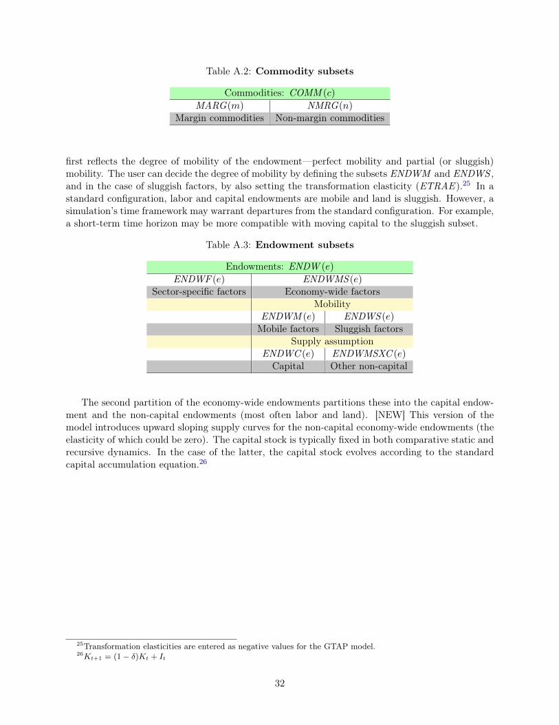
Table A.2: Commodity subsets

Commodities: COMM (c)

MARG(m) NMRG(n)Margin commodities Non-margin commodities

first reflects the degree of mobility of the endowment—perfect mobility and partial (or sluggish)mobility. The user can decide the degree of mobility by defining the subsets ENDWM and ENDWS ,and in the case of sluggish factors, by also setting the transformation elasticity (ETRAE ).25 In astandard configuration, labor and capital endowments are mobile and land is sluggish. However, asimulation’s time framework may warrant departures from the standard configuration. For example,a short-term time horizon may be more compatible with moving capital to the sluggish subset.

Table A.3: Endowment subsets

Endowments: ENDW (e)

ENDWF (e) ENDWMS (e)Sector-specific factors Economy-wide factors

MobilityENDWM (e) ENDWS (e)Mobile factors Sluggish factors

Supply assumptionENDWC (e) ENDWMSXC (e)

Capital Other non-capital

The second partition of the economy-wide endowments partitions these into the capital endow-ment and the non-capital endowments (most often labor and land). [NEW] This version of themodel introduces upward sloping supply curves for the non-capital economy-wide endowments (theelasticity of which could be zero). The capital stock is typically fixed in both comparative static andrecursive dynamics. In the case of the latter, the capital stock evolves according to the standardcapital accumulation equation.26

25Transformation elasticities are entered as negative values for the GTAP model.26Kt+1 = (1− δ)Kt + It

32