THE WELFARE EFFECTS OF EXTREME

WEATHER EVENTS – INSIGHTS FROM THREE

APEC CASE STUDIES

Office of the Chief Economist

East Asia and Pacific Region

Pub

lic D

iscl

osur

e A

utho

rized

Pub

lic D

iscl

osur

e A

utho

rized

Pub

lic D

iscl

osur

e A

utho

rized

Pub

lic D

iscl

osur

e A

utho

rized

Pub

lic D

iscl

osur

e A

utho

rized

Pub

lic D

iscl

osur

e A

utho

rized

Pub

lic D

iscl

osur

e A

utho

rized

Pub

lic D

iscl

osur

e A

utho

rized

Vice President James W. Adams (EAPVP)

Chief Economist and Sector Director, PREM and FP, EAP

Vikram Nehru (EASPR)

Task Team Leader and Lead

Economist

Ahmad Ahsan (Office of the Chief Economist

and EASPR)

Cover photo: © iStockphoto.com

PREFACE

The question of how to design economic policies that help economies adapt to a changing climatic

environment, while reducing their contributions to it, is at the heart of economic policy making today.

To tackle this challenge, the APEC Finance Ministers launched APEC Initiative Number 9 in 2008. This

Initiative reviews current fiscal, trade, and investment policies, regulatory frameworks and capacity gaps

to address the realities of a changing climate. The implications for human welfare of extreme weather

events were further examined, as an input into the broader debate about the costs and benefits of climate

change adaptation and mitigation policies. The study was coordinated by the World Bank with the support

of the Treasury of Australia. The findings are synthesized in a report entitled ―Climate Change and

Economic Policies in APEC – Synthesis Report‖. The report, together with the associated background

papers, was presented for feedback to the APEC Senior Finance Officials Meetings in September, 2010

and discussed at the APEC Finance Ministers‘ Meetings in November, 2010.

The overall study was organized in four pillars: 1) fiscal options to address climate change; 2)

technological options and role of trade and investment policies in fostering them; 3) capacity needs

assessments; 4) the human welfare effects of extreme weather events. To enable more in depth

understanding of the methodologies used and the country specific insights emerging, the background

papers underpinning each of the four pillars have been compiled in separate reports. This report provides

an in-depth review of the empirical findings emanating from three country case studies examining the

welfare effects of extreme weather. It concerns the occurrence of droughts in Indonesia, rainfall and

temperature volatility in Mexico and droughts, floods and hurricanes in Vietnam. This pillar was prepared

by a team led by Luc Christiaensen (EASER) and Emmanuel Skoufias (PRMPR) under overall guidance

of Ahmad Ahsan (Office of the Chief Economist, East Asia and Pacific). The team members included

Hector V. Conroy (IADB), Quy Toan Do (DECRG), B. Essama-Nssah (PRMPR), Roy Katayama

(PRMPR), Timothy Thomas (IFPRI), Le Dang Trung (Copenhagen University), and Katja Vinha

(PRMPR). Syud Amer Ahmed (EASPR/DECAR) and Luc Christiaensen prepared the final version of

this synthesis report.

TABLE OF CONTENTS

1. INTRODUCTION ................................................................................................................................ 3

1.1 Getting ready for extremes .................................................................................................................. 3

1.2 Extreme events do not necessarily turn into welfare loss ................................................................... 4

1.3 Innovative tools are needed ................................................................................................................. 6

1.4 Emerging insights .................................................................................................................................. 8

1.5 Moving ahead .................................................................................................................................... 10

2. INDONESIA ....................................................................................................................................... 13

2.1 Introduction ....................................................................................................................................... 13

2.2 Methodology ..................................................................................................................................... 14

2.3 Data ................................................................................................................................................... 16

2.4 Empirical Results .............................................................................................................................. 18

2.5 Concluding Remarks ......................................................................................................................... 23

3. MEXICO ............................................................................................................................................. 25

3.1 Introduction ....................................................................................................................................... 25

3.2 Past Research .................................................................................................................................... 26

3.3 Estimation Strategy ........................................................................................................................... 31

3.4 Background and Data Sources .......................................................................................................... 32

3.5 Results ............................................................................................................................................... 41 3.6 Discussion and Conclusions ............................................................................................................. 58

4. VIETNAM .............................................................................................................................................. 61

4.1 Natural Disasters and Welfare .......................................................................................................... 61

4.2 Mapping Natural Hazards ................................................................................................................. 63

4.3 Identifying Welfare Effects from Natural Disasters ......................................................................... 68

4.4 Towards an Empirical Application ................................................................................................... 70

4.5 Welfare Effects of Natural Disasters in Vietnam .............................................................................. 73

4.6 Concluding Remarks ......................................................................................................................... 77

BIBLIOGRAPHY ..................................................................................................................................... 104

APPENDIX A ........................................................................................................................................... 114

APPENDIX B ........................................................................................................................................... 124

Tables:

Table 1.1: Average costs of natural disasters per reported event (1960-2009) ............................................. 3 Table 1.2: Individuals and governments, prevent, insure and cope with extreme weather events ............... 6 Table 2.1 Summary Statistics for Households in Rural Java (1999/2000 IFLS) ........................................ 19 Table 2.2 Regression Results of Shocks on Household Consumption in Rural Java, 1999/2000 .............. 20 Table 2.3 Moderating Effects of Community-Based Programs for Households in Rural Java Exposed to

Post-Onset Low Rainfall Shocks: Average Treatment Effects based on Propensity Score

Matching ................................................................................................................................... 22 Table 3.1 Impact of weather conditions on consumption and health outcomes in rural areas .................... 30

Table 3.2 Prevalence of weather shocks in Mexican municipalities between 1986 and 2002 from mean

1951 to 1985 weather ................................................................................................................ 36 Table 3.3 Deviations from 1951 to 1985 mean weather in rural MxFLS municipalities in 2001/2002 ..... 36

Table 3.4a Weather shocks in MxFLS sample ........................................................................................... 37

Table 3.4b Weather shocks in ENN sample ............................................................................................... 37

Table 3.4 Correlations between weather shock variables and average (1951-1985) weather .................... 38

Table 3.5 Agricultural production in Mexican states included in the MxFLS ............................................ 39 Table 3.6a Select characteristics of localities in MxFLS sample ................................................................ 40

Table 3.6b Select characteristics of localities in ENN sample .................................................................... 40

Table 3.7 Weather shocks and expenditures per capita .............................................................................. 43 Table 3.8a Per capita expenditures (ln) on non-health items ...................................................................... 46

Table 3.8b Per capita expenditures (ln) on food ......................................................................................... 47 Table 3.9a Per capita (ln) expenditure on non-health items ........................................................................ 48

Table 3.9b Per capita (ln) expenditure on food ........................................................................................... 49

Table 3.10 Characteristics of rural children ................................................................................................ 52 Table 3.11 Number of observations for different sub-populations and types of weather shocks ............... 53 Table 3.12 Impact of weather on child's height-for-age ............................................................................. 54 Table 3.13 Impact of weather shocks on height-for-age, by sex ................................................................ 55 Table 3.14 Impact of weather shocks on height-for-age, by mother's education ........................................ 56 Table 3.15 Impact of weather shocks on height-for-age, by participation in a nutritional supplement

program ..................................................................................................................................... 57 Table 4.1 Extreme weather events can have substantial negative effects on household welfare,

immediately and through adaptation over time, with adaptation and disaster relief often

mitigating the immediate losses ................................................................................................ 90 Table 4.1 Extreme weather events can have substantial negative effects on household welfare,

immediately and through adaptation over time, with adaptation and disaster relief often

mitigating the immediate losses ................................................................................................ 96

Figures: Figure 1.1 Number of droughts, floods and storms in APEC economies (1960-2009) ................................ 5 Figure 1.2 Geographical distribution of the likelihood of extreme weather in Vietnam .............................. 9 Figure 2.1 Timing of typical climate events and the IFLS3 ....................................................................... 15 Figure 2.2 Variation in monsoon onset and post-onset rainfall .................................................................. 17 Figure 3.1 Environment, health and consumption relationships ................................................................. 27 Figure 3.2 Agricultural Cycle in Mexico ................................................................................................... 33 Figure 4.1 Regions of Vietnam ................................................................................................................... 79 Figure 4.2 Rainfall maps using inverse distance weighing and inverse elevation difference weighting

display close resemblance ......................................................................................................... 80 Figure 4.3 Deviations from median annual rainfall for each year 2001 to 2006. ....................................... 81 Figure 4.4 Proportion of years with 20 percent shortfall in median annual rainfall ................................... 82 Figure 4.5 Localized flooding for each year 2001 to 2006. ........................................................................ 83 Figure 4.6 Proportion of years in which 300 mm of rain fell in a consecutive 5-day period...................... 84 Figure 4.7 Riverine and coastal flooding for each year 2001 to 2006. ....................................................... 85 Figure 4.8 Proportion of riverine and coastal flooding 1985-2007. ........................................................... 86 Figure 4.9 Hurricane force winds associated with tropical cyclones for 2001 to 2006. ............................. 87 Figure 4.10 Proportion of years with hurricane force winds ...................................................................... 88

Figure 4.11 Most people are exposed to droughts, but infrequently; floods affect a sizable population

often, and large population never; hurricanes pass by most and infrequently affect others .... 89

1

EXECUTIVE SUMMARY

1. As the frequency and intensity of natural disasters increases, it is important to better

understand how extreme weather events affect economies and their people. This requires more in

depth knowledge about the exposure of different areas to these disasters, the expected costs associated

with their occurrence, and the effectiveness of different measures that help households prevent or mitigate

the effects of these events or help them cope ex post. To do so, three country case studies (Indonesia,

Mexico, and Vietnam) were undertaken, under the umbrella of an overall study on Climate Change and

Economic Policies in APEC. This study was commissioned by the APEC Finance Ministers under APEC

Initiative number 9 and has been coordinated by the World Bank.

2. This report uses new measures of extreme weather and methodologies to gauge their

welfare effects. A myriad of methodological issues and data constraints plague empirical work on the

effects of extreme weather events on human welfare. The shocks themselves are often poorly measured

and the lack of sufficiently long panel data or historical data on past events often forces a focus on effects

in the short run. Economy wide effects of local shocks are typically only explored within the context of

computable general equilibrium models which are very structural in nature. Proper evaluation of public

interventions requires correction for the unobserved characteristics of the areas which receive the

programs. The necessary baselines and control groups are also often not present. Even though many of the

challenges will remain unaddressed, the three country case studies use innovative measures of extreme

weather events derived directly from meteorological records, their historical incidence as well as

advanced econometric techniques to overcome some of these shortcomings. They examine the effects of

the timing and quantity of rainfall in rural Indonesia, the effects of too much and too little rainfall and

growing days in rural Mexico and the effects of droughts, (riverine and flash) floods, and storms in

Vietnam.

3. The key insights emerging from these studies are:

a) Natural hazard maps derived from meteorological records can be a powerful and relatively

inexpensive tool for disaster impact analysis and policy planning.

b) There is enormous geographic variation in exposure to extreme weather events, highlighting the

need for tailored analysis and interventions.

c) Households in disaster prone areas tend to be substantially poorer, even though they also tend to

be less affected by current events, especially floods.

d) The immediate human welfare effects from extreme events can be substantial (between 15 and 20

percent for shortages of rains and up to 50 percent in case of hurricanes), but differ by event,

across space and socio-economic groups, underscoring the need for disaggregated analysis.

e) Irrigation helps substantially in alleviating the effects of droughts.

f) Community based programs to mitigate risks ex ante proved effective in Indonesia.

g) Safety nets and coping strategies may help, but are not always sufficient. More rigorous impact

evaluation is needed.

2

h) Country specific points:

a. Indonesia. The community based approach, especially credit and public work projects,

was found to be a promising way forward to moderate the effects of shortfalls in rain in

rural Indonesia.

b. Mexico. The heterogeneous impact of rain and temperature variability suggests that a

―tailored‖ approach to designing programs aimed at increasing the capacity of rural

households to adapt to climate change is likely most effective.

c. Vietnam. How to better protect households against the damaging forces of hurricanes is

an important area in need of more attention in Vietnam.

4. Despite these important pointers, many questions remain about their robustness under

different assumptions and settings. In particular, important value can be added by building on the work

in the following directions.

a) The disaster mapping methodology illustrated in the Vietnam case study provides a useful

tool for policy making, project planning and disaster impact analysis. It is relatively

inexpensive to apply. Fine-tuning and validating this methodology in other settings is

recommended.

b) Despite numerous studies undertaken over the past two decades, including the ones presented

here, the empirical (and theoretical) knowledge base for choosing between different strategies

to reduce the losses from extreme events (e.g. avoiding floods or learning to live with floods)

remains thin, especially when it comes to guiding country specific interventions. A more

systematic incorporation of evaluation considerations (baseline data collection, control

groups) at the outset of new safety net projects is recommended. The model followed during

the launch of the PROGRESA program in Mexico may serve as a practical example.

3

1. INTRODUCTION

1.1 Getting ready for extremes

1. The available evidence suggests that damage from extreme weather events can be substantial. When

winds become too strong, temperatures too hot or cold and rainfall too little or too much, the assumption

is that they also cause substantial damage to people, livelihoods and economies alike. That is, they

translate into disasters. The damage estimates recorded in the Emergency Database (EM-DAT) 1 bear this

out, with the worldwide average economic damage for each storm since 1960 estimated at about half a

billion dollar and about 3.7 million people affected on average per drought (Table 1.1). In APEC

economies the estimated damage is even more severe. About 4.3 million people are affected by drought,

storms cause US$ 0.7 billion in damage on average and the number of people affected by floods is twice

this in the rest of the world. The estimates can even rise as high as US$ 125 billion in economic damage

for the most pernicious storm ever recorded (Hurricane Katrina, US, 2005), US$ 30 billion for the most

damaging flood (China, 1998) and an estimated 300 million people affected by the 1987 drought in India..

Table 1.1: Average costs of natural disasters per reported event (1960-2009)

Disaster type Number of

events*

Average

number of

people affected

Average

economic

damage per

event (US$)***

Average

number of

people affected

when economic

damage

reported

Average

economic

damage per

person

affected (US$)

World

Drought 550/155 3,707,569 571,743,265 11,066,609 52

Flood 3536/1255 877,762 346,909,622 2,471,885 140

Storm 3015/1509 280,419 504,035,783 560,280 900

APEC Economies**

Drought 113/47 4,305,199 1,059,308,362 9,860,772 107

Flood 1095/521 1,631,112 439,063,885 3,425,640 128

Storm 1533/866 399,905 679,829,779 707,913 960

Source: EM-DAT

Note: *Number of events / Number of events for which economic damage is reported; **APEC economies include

Australia, Brunei Darussalam, Canada, Chile, People's Republic of China, Hong Kong, China, Indonesia, Japan,

Republic of Korea, Malaysia, Mexico, New Zealand, Papua New Guinea, Peru, The Republic of the Philippines, The

Russian Federation, Singapore, Chinese Taipei, Thailand, United States of America, and Vietnam; *** the average

economic damage per event is calculated by dividing the total economic damage by event by the number of events

that are reported with damage. So, if there is a low reporting rate then that increase the average damage per event, as

in the case of droughts. It should also be noted that in the case of multi-year droughts, only the first year of the

drought is reported as an event.

2. The EM-DAT data also shows that the impressions left on people and economies differ considerably by

type of event. Many more people are affected by droughts than by storms, while floods tend to cause

much more economic damage than floods. This results in a widely divergent array of estimated damage

per person, going from an average of about US$ 900 per affected person over the past 50 years when it

1 EM-DAT is the world‘s most complete and widely consulted database on disasters maintained by the Centre for

Research on the Epidemiology of Disasters (CRED) since 1988, with 18,000 mass disasters recorded and records

going back to 1900. The database is compiled from various sources, including UN agencies, non-governmental

organizations, insurance companies, research institutes and press agencies.

4

comes to storms around the world to U$140 estimated damage per affected person from floods. The

differential effect on human and physical capital from droughts, floods and storms has important

implications for their effects on economic growth and human welfare. It also affects the benefits from

different measures (risk reduction, risk mitigation, risk coping) in dealing with them.

3. Despite these numbers, our understanding of how much extreme weather affects people, livelihoods

and economies and for how long remains poor. While EM-DAT provides the most comprehensive and

widely consulted database to date on disasters and their damages, these estimates remain inevitably partial

and incomplete. Not only is damage assessment notoriously difficult, it is often largely based on estimates

of asset damage, ignoring the complexity and ingenuity of human behavior in the face of natural hazards.

More refined answers to the question of the welfare costs associated with extreme weather events are

needed to assess the benefits from investments and policies to reduce people‘s exposure to these events or

to strengthen their capacity to cope with them ex post. In designing such interventions it is equally

important to better understand the short and long run consequences of extreme weather events and map

which population groups and regions are more or less likely to be affected.

4. Better quantification of the effects of extreme weather events is important as they are not singular, and

likely to occur more frequently as climate change proceeds. A review of the number of droughts, floods

and storms in the APEC economies suggests that the number of events has trended upward over the past

five decades (Figure 1.1). Looking forward, as the globe warms up, the frequency of these events and

their associated damages are predicted to increase even further (United Nations and World Bank, 2010).

Rising sea water levels for example increase flood risks and climate change shortens the return period of

large storms, in effect fattening the tail of the damage distributions of large storms. In addition, the

occurrence of multiple smaller hardships or disruptions from climate change over a shorter period could

erode coping systems and combine to cause even greater damage than the sum of each event on its own.

While the timing, bunching and coincidence of the different extreme events remains essentially unknown,

their effects could be substantially mitigated through proper preparation. To better appreciate the

importance of being prepared, it is important to understand the channels through which extreme weather

events affect people, livelihoods and economies and how households, communities and governments have

so far managed their impacts.

1.2 Extreme events do not necessarily turn into welfare loss

5. A framework is needed to understand whether extreme events translate into welfare loss. The expected

losses from extreme events are modulated by government policies and individual responses taken before

and after the events occur. Ignoring the implicit or explicit individual, community or government outlays

involved in these responses underestimates the true costs associated with extreme weather events. To

better grasp the full effect of extreme weather events, a simple framework is proposed to disentangle the

channels through which households try to shield themselves from their effects. The organizing framework

used here goes back to the social risk-vulnerability chain pioneered by Heitzmann et al. (2002) and Siegel

et al (2003).

6. Smoothing incomes through risk prevention: The risk of an extreme weather event happening differs

across space. However, even when it materializes, not everybody will be equally affected. The likelihood

of an event happening and the sensitivity of a household‘s income to it determine together the actual

exposure of the household. Preventing the event from happening, or more precisely, preventing the event

from affecting one‘s income stream, is one widely applied strategy to reduce exposure to natural hazards.

Use of irrigation in drought prone areas is just one example. By taking direct control of the water supply,

households insulate their harvests and incomes from the vagaries of the rains. Doing so not only reduces

the volatility of their incomes, it may also increase yields on average, for example by enabling multiple

5

harvests per year. Risk prevention also happens through income and asset portfolio diversification. Such

a strategy, however, often comes at the expense of lower average – but more stable – income streams.

Figure 1.1: Number of droughts, floods and storms in APEC economies (1960-2009)

Source: EM-DAT data

7. Smoothing incomes through insurance or risk mitigation: Risk prevention strategies seek to reduce

risks by reducing the exposure and sensitivity of one‘s asset and income portfolio to the event itself.

Another set of ex ante strategies seeks to set up arrangements for compensation in case of the event

materializes, i.e. it seeks to stabilize incomes ex post by insuring them ex ante. They also go under the

name of risk mitigation strategies. This can be done through savings (self-insurance) or through (formal

or informal) market insurance arrangements. Insurance markets are however often incomplete, especially

in developing economies. Risk prevention and mitigation strategies are in essence aimed at smoothing

incomes by taking action ex ante, before the event strikes.

8. Smoothing consumption ex post through risk coping, even when incomes are volatile: In addition to

smoothing and insuring incomes ex ante, households often also have to undergo the shock and try to cope

with income losses ex post to maintain their consumption. A myriad of strategies have been deployed by

households to do so, including temporal migration, drawing down of stocks of social and human capital,

or dietary shifts to cheaper calories. Together these individual risk prevention, mitigation and coping

strategies help households smooth their consumption and reduce the welfare effects from extreme weather

events.

9. Community and government/donor interventions further complement individual/household risk

prevention, compensation and coping strategies. Community infrastructure projects can for example

reduce the threat of floods and landslides, while the institution of enforceable property rights (e.g. of land

and trees) can provide the needed incentives for afforestation and drought reduction as observed in Niger.

Extreme weather events tend to cause less damage when capital markets are better developed. In the

absence of such markets, savings and credit cooperative associations can facilitate precautionary saving.

Catastrophic bonds are increasingly used by governments to insure their outlays in case of extreme

6

events. To cope with shocks ex post, households often fall back on remittances (domestic and

international), especially when public safety nets and disaster relief funds are poorly developed and

inadequate. These can be effective. Children under two in drought affected communities in Ethiopia saw

their growth slow down almost by one centimeter over a 6 month period, though not in communities that

also received food aid (Yamano et al., 2005). Yet, many children were left stunted nonetheless because

poor targeting rendered food aid rather unresponsive to drought shocks.

Table 1.2: Individuals and governments, prevent, insure and cope with extreme weather events

Measure Individuals/households Community Governments

Risk reduction or

prevention

Owning multiple assets and

diversifying sources of income

Irrigation

Investments to protect and

maintain assets (timely repairs)

Permanent migration

Community training

Community-based

information systems

Small scale

irrigation and

infrastructure

projects

Development of better

information systems (disaster

risk profiles, early warning

systems, public awareness

raising)

Public works

Enforceable property rights

Risk mitigation

or insurance

Self insurance through saving

(cash, livestock, grain storage,

durables)

Market insurance such as

weather/catastrophe based

insurance for property, crops

Local borrowing and

saving schemes

Microfinance

Cereal banks

Well functioning markets (e.g. to

sell livestock)

Sovereign budget insurance and

catastrophe bonds

Safety nets (cash transfers and

public employment guarantee

schemes)

Deferred Draw Down Options

(DDO)

Risk coping or

ex-post risk

management

Temporal migration or expansion

of household labour

Drawing on stocks of social capital

or human capital

Diversifying expenditures towards

less expensive calories and goods

Interhousehold

transfers and private

remittances

Disaster relief

Source: United Nations and the World Bank (2010)

1.3 Innovative tools are needed

10. The effects of natural shocks and the effectiveness of different instruments and strategies in dealing

with them remain poorly quantified, because of methodological challenges and data constraints. A myriad

of methodological issues and data constraints plague our empirical understanding of the effects of

extreme weather events on human welfare. The shocks themselves are often poorly measured and the lack

7

of sufficiently long panel data or historical data on past events often forces a focus on the short run.

Economy wide effects of local shocks are typically only explored within the context of computable

general equilibrium models which are very structural in nature. Proper evaluation of public interventions

requires correction for the unobserved characteristics of the areas that receive the programs, but baselines

and control groups are often not present. The three country case studies presented in this report remedy

some of these shortcomings using weather and climate data, though many of the challenges will remain

unaddressed. The case country studies focus on the effects of the timing and quantity of rainfall in rural

Indonesia, the effects of too much and too little rainfall and growing days in rural Mexico and the effects

of droughts, (riverine and flash) floods, and storms in Vietnam.2

11. Subjective versus objective measures of extreme weather: Subjective measures of shocks are often

used to identify whether households have been affected by extreme weather or not. They consist of self

reported declarations of having experienced a shock by the households or communities. Such information

is regularly recorded in standard household questionnaires and avoids having to define a cut-off beyond

which rain, wind or temperature is considered either too high or too low. Yet, as seen above, whether a

household considers a meteorological event a disaster is likely to depend both on its ex-ante exposure to it

as well as its ex-post capacity to cope with it. To reduce its exposure it may have adopted less risky

portfolio strategies over time. As a result, it may not consider the event a shock because it has already

adapted to it, leading to an underestimate of the true welfare loss associated with shocks. Moreover, it is

typically also difficult to extrapolate the findings across space and time, as subjective shock measures are

usually not available outside the sample, and neither are their probability distributions. The latter are

especially useful to explore their long run effects and to simulate the effects of climate change. The

country case studies presented here use objective measures of extreme weather, derived directly from the

meteorological data, as opposed to subjective measures, based on household reports. This required

innovative methods to interpolate the meteorological event data across space and to link them to the

economic data sources on household assets, income, and consumption and human development outcomes.

12. Measuring both the long and short of it: The effects of current events may not only be felt today, but

also long thereafter. That there is long run detrimental damage of growth retardation during the first 1000

days of life (from conception to the age of 2) has been well documented.3 There is less evidence and

consensus of the long run effects of extreme weather events on economic growth4 or household welfare

5.

To speak to this issue, the Vietnam case study explores the welfare effects of past weather events, in

addition to the current ones. It further examines the welfare effects of regular exposure to extreme events,

in effect capturing the cumulative effects of those events as well as those of any adaptation strategies (e.g.

more drought resistant varieties, flood proof crops) adopted over time to mitigate their effects.

13. Extreme weather events affect incomes directly as well as indirectly, through their effects on the rest

of the economy. Droughts for example, affect farmers‘ incomes directly through harvest loss. Yet, they

may also affect other consumers indirectly, through the food and factor markets. Food prices may

increase affecting net rural buyers and urban consumers and the demand for agricultural wage labor may

decrease (Jayachandran, 2006). Similarly, while hurricanes destroy assets, they may subsequently also

generate employment opportunities in the construction industry, following reconstruction. While the

indirect effects may often be more important than the direct effects (Okuyama, 2009), they are typically

2 Skoufias et al. (2011a), Skoufias et al. (2011b), and Thomas et al. (2010)

3 One such study is by Maccini and Yang (2009) who find significant (negative) effects of rainfall during early life

between 1953 and 1974 on future schooling, health and socio-economic indicators of women in rural Indonesia. 4 Cavallo and Noy (2010) and Loyaza, Olaberria, Rigolini and Christiaensen (2009) review the literature regarding

the effects of natural disasters on economic growth and conclude that it is largely inconclusive, with some studies

suggesting a negative effect on growth, others no effect and a few, even a positive effect. 5 Dercon (2004) forms a welcome exception, reporting that household hit hard by the 1984-5 famine in Ethiopia

experienced 16 percentage points less growth in their consumption between 1989 and 1997 compared with those

household who weren‘t hit by the drought.

8

ignored in the econometric analysis. The importance of controlling for the indirect effects in exploring the

direct ones is illustrated in the Vietnam case study.

14. Innovative tools to explore the welfare impacts of weather events and the effectiveness of some of the

prevention, mitigation and coping strategies. To examine the welfare effects of extreme events each case

country study spatially interpolates the extreme events derived from meteorological data. In doing so, the

Vietnam study goes one step further, constructing explicit hazard and event maps. These disaggregated,

geo-referenced hazard maps are subsequently coupled with detailed geo-referenced household survey data

of income, consumption, and human development measures to statistically estimate the impact of weather

shocks on these measures. In Indonesia, the focus is on the timing of the rainfall, and in Mexico both

extreme temperatures and rainfall patterns are considered. In each study, the effects on rural households

and incomes are analyzed, mainly via the agricultural channel. The Vietnam study is more

comprehensive in scope, considering droughts, localized and riverine floods as well as storms and

considers both rural and urban areas. Each study further explores differences in impacts across

geographical areas and socio-economic groups. In addition, the effectiveness of irrigation and a series of

safety net and community relief programs is also explored. Finally, the Vietnam case study also

distinguishes between the short and long run effects, controls for indirect effects, and documents some of

the channels through which households try to mitigate the effects of extreme weather events (including

asset decumulation, reception of domestic and international remittances, and disaster relief).

1.4 Emerging insights

15. The natural hazards maps illustrate the enormous geographic variation in exposure to extreme weather

events. A recurring finding across the case studies is the spatial variation in exposure to different events.

This is best illustrated by the hazard maps constructed for Vietnam (such as Figure 1.2). The maps also

provide an important tool for planning and gauging the exposure of interventions to extreme events. In

one application, they were overlaid with World Bank sponsored projects, indicating the extent to which

the World Bank portfolio was exposed.6

16. The human welfare effects from extreme events can be substantial, but differ by event, across space

and socio-economic groups, underscoring the need for disaggregated analysis. Focusing on irregular

rainfall patterns, the evidence from rural Java, Indonesia suggests for example a decline in per capita

consumption by 17 percent among rice farmers, when the rains are two standard deviations below their

mean during the 90 day post-monsoon onset period. While negative, the effect on other households was

however not statistically significant. Similar declines in welfare following droughts (14-17 percentage

points) are reported for Vietnam, at least when the fields are not irrigated. Yet, in Mexico, there was no

evidence of consistently negative effects of droughts, heat waves or cold weather, even though significant

differences were noted across regions (North versus Center and South) and socio-economic groups (with

female headed households for example better able to benefit from positive weather shocks). Hurricanes

(explored only in Vietnam) caused most damage, with households in metropolitan centers seeing their

welfare go down by 50% when hit by a hurricane. Riverine floods in Vietnam also caused substantial

welfare loss in the short run (up to 23 percent). The losses are again smaller the further away from the

metropolitan centers households are, possibly because economies are less integrated in more remote

settings. Finally, the Mexico case study also explored the effects of extreme precipitation and temperature

on child health. Contrary to expectations, it was during wet and hot years that boys (but not girls) saw

their nutritional status go down, and then especially in the center and south of Mexico, underscoring the

differentiated nature of the impact of extreme events.

6 http://115.146.126.6:8008/

9

Figure 1.2: Geographical distribution of the likelihood of extreme weather in Vietnam

Source: Thomas et al. (2010)

17. Irrigation helps substantially in alleviating the effects of droughts. The results from both Indonesia

and Vietnam show that irrigation is effective in shielding households from the effects of droughts. They

were basically unaffected. This underscores that irrigation may not only increase annual yields (for

example by enabling multiple harvests per year), but that an important contribution also comes from

helping households smooth their income and consumption over time, an important additional benefit.

18. Households in disaster prone areas tend to be substantially poorer, even though they also tend to be

less affected by current events, especially floods. A core finding from the Vietnam study is that regular

exposure to disasters poses an important drag on households‘ welfare. Cumulative asset loss and

adaptation likely erode the asset base and induce the adoption of lower risk, lower return portfolios over

time. However, in areas where rivers frequently exceed their banks, households appear richer. This is

specifically for households in the Mekong River Delta that have learned to live with floods and have built

their livelihood systems around them. Yet, regular exposure to shocks also prepares households better for

the next event, reducing the immediate effects of extreme events, especially when it comes to floods. This

does not apply to hurricanes, with regular exposure in effect exacerbating the already disastrous

consequences from current events. Frequent exposure to hurricanes erodes the capacity of households to

cope with such events and government relief programs have so far not been very effective in providing

relief.

19. Community based programs to mitigate risks ex ante prove effective in Indonesia. It is the

availability of credit (provided through the INPRES Poor Villages Program) that proved most effective in

reducing the effects of rainfall shocks in Indonesia, followed by the community based infrastructure

development programs.

20. Safety nets and coping strategies may help, but are not always sufficient. The community based

programs in Indonesia developed in response to the 1997-98 crisis (such as its labor intensive public work

programs and its village infrastructure block grant programs) provided a useful cushion to rainfall failure.

10

The Vietnam study also provides indirect evidence that disaster relief systems are instrumental in

mitigating the effects of extreme weather events. The Mexico study on the other hand, concludes that the

current risk-coping mechanisms (public and private) are not effective in insulating rural household

welfare and child health from erratic weather patterns (as measured by annual precipitation and growing

degree days). While providing useful pointers, given data limitations, the case country studies were not

able to provide a rigorous assessment of the safety net programs. This is an area in dire need of more in

depth analysis, including regarding the effects of the design of such programs on their effectiveness.

1.5 Moving ahead

21. Deepening and fine-tuning our understanding of how natural disasters affect human welfare is a

pressing concern, as climate change is set to increase the frequency and severity of weather shocks. This

requires more in depth knowledge about the exposure of different areas to these disasters, the expected

costs associated with their occurrence, and the effectiveness of different risk prevention, mitigation and

coping measures. The following lessons emerge from the three case studies.

a) Geographically disaggregated natural disaster maps from meteorological data provide a useful

tool for policy making, project planning and disaster impact analysis. The methodology illustrated

here for the Vietnam case study provides a relatively inexpensive and promising method to do so.

Fine-tuning and validating this methodology in other settings is thus worthwhile. This is

quintessentially a multi-disciplinary (scientists and economists) and cross-sectoral effort, a

continuing challenge in our mono-discipline focused world. Nonetheless, the current efforts

provide a good starting point to build on.

b) The estimated long run effects are huge, especially for droughts and hurricanes, while the short

run effects are highly varied, highlighting the need for a better and more granulated

understanding of the relative effectiveness of the different prevention, mitigation and coping

options. Despite the numerous studies undertaken over the past two decades, including the ones

presented here, the empirical (and theoretical7) knowledge base for choosing between different

strategies (e.g. avoiding floods or learning to live with floods) remains thin, especially when it

comes to guiding country specific interventions. The myriad of safety net and community based

initiatives that are being introduced across the APEC economies provide a unique learning

opportunity to expand and tailor the knowledge base. It would require a much more systematic

incorporation of evaluation considerations (baseline data collection, control groups) at the outset

of the projects. This would in turn enable a much more refined response to important questions

regarding design issues of safety nets as well as cost benefit analysis. The model followed during

the launch of the PROGRESA program in Mexico provides a good example to build on.

c) Country specific insights include:

a. Indonesia. The community based approach, especially credit and public work projects were

found to be a promising way forward to moderate the effects of shortfalls in rain in rural

Indonesia.

b. Mexico. The heterogeneous impact of rain and temperature variability suggests that a

―tailored‖ approach to designing programs aimed at increasing the capacity of rural

households to adapt to and mitigate the effects of climate change is likely most effective.

7 Devarajan and Jack (2007) is an important and insightful exception.

11

c. Vietnam. While irrigation helps mitigate the effects of droughts, and disaster relief takes

some of the sharp edges away from heavy rains and riverine floods, households largely

undergo the effects of hurricanes, with little relief from effective adaptation or ex post coping

strategies, especially for those in areas close to the metropoles. How to better protect

households against the damaging forces of hurricanes is an important area in need of more

attention in Vietnam.

The remainder of the report discusses each of the three country case studies in more detail.

12

13

2. INDONESIA

2.1 Introduction

1. The adverse impacts of climate change8 and extremes represent a serious challenge to development

efforts around the globe and are likely to exacerbate the incidence, severity and persistence of poverty in

many countries. The global mean surface temperature of the earth has been rising as a result of increased

emission of greenhouse gases, particularly carbon dioxide (DFID 2004). Climate change and extremes are

expected to affect mostly climate-sensitive sectors of the economy and in turn influence the pattern of

household income and consumption. It is estimated that three-quarters of the world‘s poorest whose

standard of living falls below $2 per day rely mostly on natural resources for their livelihoods (WRI,

2008). The degradation of natural resources induced by climate change thus places significant stress on

these livelihoods. As for agriculture, an important sector of activity for the poor, yields from rain-fed

agriculture could be cut by half by 2020 in some parts of the world. It is feared that climate change could

reduce soil fertility by 2 to 8 percent, inducing a significant reduction in yields for a variety of crops.

2. However, very little is known about the welfare losses that households experience from these

phenomena. Households at low levels of income are believed to be the most vulnerable to the impacts of

climate change and extremes. This is due to their geographical locations, limited assets, limited access to

resources and services, low human capital and high dependence upon natural resources for income and

consumption. While there is wide recognition of this impending threat of climate change upon the poor,

limited attention is given upon quantifying the poverty and distributional effects of climate change and

identifying adaptation strategies and targeted measures that could mitigate the poverty impacts.

3. This chapter analyzes the potential welfare impacts of rainfall shocks in rural Indonesia, and draws

relevant policy lessons. With an estimated population of 237.5 million, Indonesia is the largest

archipelago and the fourth most populous nation in the world. Located in Southeastern Asia between the

Indian and the Pacific Oceans, the country has a tropical climate with two distinct seasons, monsoon wet

and dry, and is endowed with high levels of biodiversity. The country has been experiencing change in

both mean temperature and precipitation. Since 1900, it is estimated that the annual mean temperature has

increased about 0.3o C. 1998 was the warmest year in the century as the temperature rose 1

o C above the

1961-1990 average (PEACE 2007). The increase in average temperature is projected to lie between 0.36

and 0.47o C by the year 2020. It is reported that overall annual precipitation has decreased by 2 to 3

percent, but there are significant regional differences (WWF, 2007). Southern regions such as Java,

Lampung, South Sumatra, South Sulawesi, and Nusa Tenggara have seen a decline in annual rainfall.

Northern regions on the other hand have experienced an increase in precipitation. These include most of

Kalimantan and North Sulawesi. These changes in precipitation are strongly influenced by El Niño

Southern Oscillation (ENSO). Indonesia tends to experience droughts during the warm phase of ENSO

(i.e. El Niño) and excessive rain in the cool phase (i.e. La Niña). With the possible exception of southern

Indonesia annual rainfall is expected to increase across the rest of the country (Naylor et al., 2002).

8 According to the Intergovernmental Panel on Climate Change (IPCC) a narrow definition of climate refers to the

statistical description in terms of the mean and variability of quantities such as temperature, precipitation and wind

over a period of time ranging from months to thousands of years. The norm is 30 years as defined by the World

Meteorological Organization (WMO). In a wider sense, climate refers to the state and the statistical description of a

system composed of the following five components: atmosphere (gaseous envelope around the Earth), hydrosphere,

cryosphere (snow and ice), land surface, and biosphere (all ecosystems and living organisms). For more details,

please see Parry et al. (2007). Climate is different from weather which refers to atmospheric conditions in a given

place at a specific time. The term ―climate change‖ is used to indicate a significant variation (in a statistical sense)

in either the mean state of the climate or in its variability for an extended period of time, usually decades or longer

(Wilkinson 2006).

14

4. These observed and expected changes in climate are bound to have adverse impacts on the ecosystems,

the associated resources and the lives of people who rely on these resources and on agricultural activities.

The 1997-1998 droughts associated with El Niño led to massive crop failures, water shortages and forest

fires in parts of Indonesia, and likely exacerbated the impacts of the financial crisis at that time. El Niño

events tend to delay rainfall, leading to a decrease in rice planting in the main rice-growing regions in

Indonesia such as Java and Bali. Adapting projections by the IPCC to local conditions, Naylor et al.

(2007) predict that by 2050 change in the mean climate will increase the probability of a 30-day delay in

monsoon from 9-18 percent currently to 30-40 percent. This delay combined with increased temperature

could reduce the yield of rice and soybean by as much as 10 percent. The analysis presented here

considers the welfare implications of both a late monsoon onset and low level of rainfall. As noted later, a

certain amount of rainfall is needed in the 90 day post-onset for rice to grow properly.

5. The chapter is organized as follows. Section 2.2 presents the methodology focusing on the estimation

of the impacts of rainfall variability on household expenditure per capita, our measure of welfare. The

guiding view here is that the distribution of welfare losses associated with such events depends on the

degree of household and community level vulnerability and the moderating impact of existing assets and

social protection institutions. Understanding these factors plays an important role in designing policies to

minimize exposure to and the impact of these shocks. Section 2.3 describes the available data while

analytical results are presented in section 2.4. Concluding remarks are made in section 2.5.

2.2 Methodology

6. This section describes the methodology and analytical frameworks used in estimating the impacts of

rainfall variability on household welfare in rural Indonesia and the potential moderating effects of

community-based programs and infrastructure. We need to make our analytical framework consistent

with the logic of vulnerability, the bedrock concept for the study of the welfare impacts of climate change

and extremes. The distribution of economic welfare in any given society hinges crucially on individual

endowments and behavior and the socio-political arrangements that govern social interaction. These

factors (endowments, behavior and social interaction) also determine the distribution of vulnerability9.

Adger (1999) emphasizes the connection between individual and collective vulnerability because it is

impossible to consider individual achievement in isolation from the natural and social environment.

Vulnerability of an individual or a household to livelihood stress depends crucially on both exposure and

the ability to cope with and recover from the shock. Exposure is a function of, inter alia, climatic and

topographical factors. The ability to cope is largely determined by access to resources, the diversity of

income sources and social status within the community10

. Increased exposure combined with a reduced

capacity to cope with, recover from or adapt to any exogenous stress on livelihood leads to increased

vulnerability.

7. Given data limitations, we focus on exploiting cross-sectional variation in the data and linking some

welfare indicator (e.g. consumption per capita) or some component thereof (food versus non-food

expenditure) to a climate-related shock defined on the basis of available rainfall data focusing mainly on

rural households. As noted earlier, the yield of crops such as rice (staple food in Indonesia) and soybean is

very much affected by changes in precipitation patterns which are strongly influenced by ENSO.

8. Given the importance of rice farming in the rural economy of Indonesia, we define climate shocks with

reference to this activity. Naylor et al. (2007) explain that El Niño events can cause a delay in monsoon

9 Vulnerability is usually taken as the likelihood that, at a given point in time, individual welfare will fall short of

some socially acceptable benchmark (Hoddinott and Quisumbing 2008). 10

Hoddinott and Quisumbing (2008) make essentially the same point by noting that, at the household level,

vulnerability is determined by the nature of the shock, the availability of additional sources of income, the

functioning of labor, credit and insurance markets, and the extent of public assistance.

15

onset of up to 60 days. The same authors define ―onset‖ as the number of days after August 1 when

cumulative rainfall reaches 20 cm 11

, and ―delay‖ as the number of days above the mean onset date over

the 1979-2004 period. Since farmers will typically begin planting after monsoon onset, late onset may

affect prospects for a second harvest later in the season and possibly change crop combinations (with

potentially significant consequences on production and market prices).

9. While delayed onset is an important determinant of harvest, we also need to consider the amount of

rainfall after the onset. After farmers plant the rice fields, 60-120 cm of rainfall are needed during the 3-4

month grow-out period (Naylor et al., 2002). Thus, the second dimension of the shock involves the

deviation of the amount of post-onset rainfall from the 25 year mean for each weather station. The amount

of post-onset rainfall is defined as the total amount of rainfall during the 90 day period following the

monsoon onset date.

Figure 2.1 Timing of typical climate events and the IFLS3

10. The timing of these events in relation to the IFLS3 survey is illustrated in Figure 2.1. Considering that

the degree of rainfall variability can differ across areas and that households may adjust farming practices

accordingly, we use standard deviations from the inter-temporal mean to help account for such spatial

differences. In terms of delay of monsoon onset, a negative shock is defined as being more than one

standard deviation above the 25 year mean. In terms of the amount of post-onset rainfall, a negative shock

is defined as being more than two standard deviations below the 25 year mean.

11. Given the interconnection between individual and collective vulnerability and adaptive capacity, the

empirical analysis uses regressions to link an indicator of household welfare (real per capita total

expenditure or its food and nonfood components) to some climate shock while controlling for household

characteristics, and for the province of residence. A regression equation of the form described in equation

2.1 below is estimated, where Yij represents per capita household expenditure of household i in

community j, and Xi represents various control variables. Sj represents the covariate rainfall shocks, and

Fi is a binary variable representing rice farming households.

(2.1)

12. After analyzing the effects of rainfall shocks on welfare, we consider the potential moderating effect

of various community level programs. As Pitt et al. (1993) have argued, the placement of government

programs is not likely to be random. One consequence of the endogeneity in program placement is that it

is likely to result in biased estimates of program effects, especially when using cross-sectional data.

Recognizing that government assistance programs are often targeted to poor areas, we use propensity

score matching to investigate the difference that some community programs make with respect to

mitigating the impact of the shock on household welfare. In particular, the sample is restricted to

11

This is the amount of rainfall needed to moisten ground sufficiently for planting. It is believed that about 100 cm

of rain are needed throughout the season for cultivation.

16

households exposed to the post-onset low rainfall shock. In line with treatment response literature, the

treatment group consists of affected households residing in communities with a specific program or

infrastructure (e.g. technical irrigation, safety net programs, access to credit, etc.) while the comparison

group is made of affected households living in communities without such a program. Assuming that,

conditional on observable community characteristics, program placement is as good as random we can

consider two households with the same propensity score as observationally equivalent. Let one of these

reside in a community with the program.

13. The outcome of the other affected household residing in a community without the program represents

a counterfactual outcome for the one in a community with the program. Here the propensity score is the

probability of observing an affected household in a community with the program of interest as a function

of some covariates. We estimate propensity scores on covariates using probit and retrieve their predicted

values for matching ―treated‖ observations with those in the comparison group. Specifically, for each

program, a separate stepwise estimation of the probit specification was performed such that variables with

a p-value less than 0.5 were added to the right hand side. The list of possible right hand side variables for

the stepwise estimation included household and community variables. The household variables included:

household size, age of head, marital status of head, gender of head, education level of head, household use

of electricity, ownership of farmland, household nonfarm business, and household farm business. The

community variables included: availability of public transport, availability of piped water, predominance

of asphalt roads, share of households with electricity, distance to provincial capital, distance to district

capital, and the shares of household heads with elementary, junior high, high school, and university level

education.

14. Each treatment household is matched to its ―nearest neighbor‖ based on propensity scores, restricting

matches to the same year of the survey. We then compare average outcomes for affected households in

the treatment group (i.e. in communities with a specific program or infrastructure) to the average outcome

for similarly affected households in the comparison group (i.e. living in communities without the program

under consideration).

15. To describe this somewhat more formally, let Yi (1) denote the per capita expenditure outcome of

household i in the presence of some ―treatment‖ attribute in the local community, such as a safety net

program or type of infrastructure, and Yi (0) denote the per capita expenditure outcome of household i in

the absence of the attribute in the local community. As both Yi (1) and Yi (0) are not observable, we use

bias-corrected matching estimators, )0(ˆiY , in place of Yi (0) (see Abadie and Imbens, 2002, and Abadie et

al., 2004) and estimate the sample average treatment effect for the subpopulation of the treated (SATT),

as in equation 2.2, where Wi=1 indicates that a household is in a community with the treatment attribute,

and n1 is the sample size of the treated.

1|1

)0(ˆ)1(1

iWi

ii YYn

SATT

(2.2)

2.3 Data

16. We are able to study the impacts of extreme weather events on rural households by merging

household and community level data from the Indonesian Family Life Survey (IFLS) with daily rainfall

data covering a 25 year period. The combined data set contains information on rainfall, household

expenditures, household level socio-economic characteristics, and community level attributes.

17. Household and community surveys were fielded from late June to the end of October 2000 for IFLS3

and from August 1997 to January 1998 for IFLS2. The surveys include village-level data which allows

17

the determination of the extent to which access to better infrastructure or social programs increases

resiliency. The consumption aggregate consists of food and nonfood components. The food component

consists of 37 food items (purchases and the value of own production or gifts) consumed within the last

week. The nonfood component consists of frequently purchased goods and services (utilities, personal

toiletries, household items, domestic services, recreation and entertainment, transport, sweepstakes), less

frequent purchases and durables (clothing, furniture, medical, ceremonies, tax), housing, and educational

expenditures for children living in the household. Transfers out of the household were excluded. All

values are monthly figures and are in real terms. To obtain real values, both temporal and spatial deflators

were used, using prices in December 2000 in Jakarta as the base.12

18. Using daily rainfall data from 1979 to 2004, we calculated the 25 year mean and standard deviations

for monsoon onset and the amount of post-onset rainfall for 32 weather stations. The rainfall data from

these weather stations were then matched to communities in IFLS. Weather data were merged with

household survey data at the community level based on proximity. Only weather stations with complete

data for the 25 year period were used. The matched data contained a total of 267 communities and 32

WMO stations. In rural areas, 106 communities in 9 provinces were matched to 27 stations. In rural Java,

66 communities in 4 provinces were matched to 18 stations. The number of communities per WMO

station ranged from 1 to 10 in rural areas. 3,290 households were matched to 27 stations in rural areas,

and 2,159 households were matched to 18 stations in rural Java.

19. After merging available precipitation data and dropping observations with missing data, the sample

size in the 2000 IFLS3 for our analysis was reduced to 6,188 households from a total of 10, 292. 3,290

households in our 2000 sample were located in rural areas, and of these 2,159 were located on Java. Data

from additional weather stations would benefit this analysis by improving the level of disaggregation of

weather data, but this data could not be obtained.

Figure 2.2 Variation in monsoon onset and post-onset rainfall

20. Figure 2.2 shows variation by province in monsoon onset and post-onset rainfall. With respect to

delays in monsoon onset, only provinces in Java experienced a delay greater than one standard deviation

from the 25 year mean in 1999/2000. As for the amount of rainfall during the 90 day post-onset period,

the data indicate that only provinces in Java experienced rainfall below two standard deviations from the

25 year mean in 1999/2000.

12

The spatial deflator used is the ratio of the location (province, urban/rural area) poverty line (in December 2000

prices) to the Jakarta poverty line. Thus the spatial deflator used converts the local December 2000 values into

Jakarta December 2000 values.

-2-1

01

2

N. S

umat

ra

W. S

umat

ra

S. S

umat

ra

Lam

pung

Jaka

rta

W. J

ava

C. J

ava

Yog

yaka

rta

E. J

ava

Bali

S. K

alim

anta

n

N. S

umat

ra

W. S

umat

ra

S. S

umat

ra

Lam

pung

Jaka

rta

W. J

ava

C. J

ava

Yog

yaka

rta

E. J

ava

Bali

S. K

alim

anta

n

1996/1997 1999/2000

(std

. de

v.

from

25

ye

ar

me

an

)

De

lay o

f m

on

so

on

on

se

t

-50

510

N. S

umat

ra

W. S

umat

ra

S. S

umat

ra

Lam

pung

Jaka

rta

W. J

ava

C. J

ava

Yog

yaka

rta

E. J

ava

Bal

i

S. K

alim

anta

n

N. S

umat

ra

W. S

umat

ra

S. S

umat

ra

Lam

pung

Jaka

rta

W. J

ava

C. J

ava

Yog

yaka

rta

E. J

ava

Bal

i

S. K

alim

anta

n

1996/1997 1999/2000

(std

. de

v.

from

25

ye

ar

me

an

)

90

da

y p

ost-

on

se

t ra

infa

ll

18

21. The summary statistics of household expenditures, household characteristics, and rainfall shock

exposure in rural Java are shown in Table 2.1. The majority of household heads were married males who

did not have more than an elementary education. The vast majority of households utilized electricity. Half

of the households owned farmland, and 44 percent were engaged in non-farm businesses. Nearly 60

percent of households were engaged in a farm business, 38 percent with rice as the most valuable crop

and 22 percent with another crop as the most valuable. 34 percent of households in our sample were

exposed to the delay of onset shock and 45 percent were exposed to the post-onset low rainfall shock. The

correlation coefficient between these two shock variables for our sample was not large at 0.38.

2.4 Empirical Results

22. We present our findings on (i) the impact of rainfall shocks on per capita household consumption

levels and (ii) the role that various social programs may have played in mitigating the negative welfare

impacts of the rainfall shocks. For the first part, we used regression analysis to quantify the average

reduction in household welfare levels for those exposed to low rainfall shocks. For the second part, we

used propensity score matching to estimate the extent of moderating effects offered by the various

community-based programs.

Welfare Impacts of Rainfall Shocks

23. Given the importance of rain-fed agriculture, in particular rice farming, to rural livelihoods in

Indonesia, we study the potential impact of rainfall shocks on per capita total household expenditure, and

its food and nonfood components. We focus on rural Java, the predominant rice production area in

Indonesia, and use regression analysis to estimate the impacts on household expenditures.

24. We include in our regressions two binary variables representing the two rainfall shocks defined

earlier, delayed monsoon onset and post-onset low rainfall. We interact these shock variables with a

binary variable for rice farming households, specifically households engaged in a farm business with rice

as the most valuable crop. This is done to differentiate the effect of the shocks between households that

have and do not have a farm business with rice as the most valuable crop. In the regressions, we control

for various household characteristics: household size, age of household head, sex and marital status of

head, level of education of the head (binary variables for elementary, junior high, high school, and

university), access to electricity, ownership of farm land, and household farm and nonfarm business

activity, whether or not rice is the most valuable crop, and province of residence. The reference case is a

household in rural West Java province, with an uneducated, single, male head, that has no access to

electricity, no farm land, and no household farm or nonfarm businesses.

25. Using the two rainfall shock variables separately as well as together, we used three different

specifications for our regressions. The first includes a binary variable for delayed monsoon onset along

with its interaction term with the binary variable for rice farming household. The second substitutes the

post-onset low rainfall variable as the shock variable. The third includes both rainfall shocks along their

interaction terms. This third variation was used with different dependent variables, that is, per capital total

household expenditure and its food and nonfood components.

19

Table 2.1 Summary Statistics for Households in Rural Java (1999/2000 IFLS)

26. As might have been expected, there is a strong positive correlation between household per capita

expenditure and assets; education and ownership of farmland. All education coefficients are positive and

significantly different from zero. For all five of the regressions reported in Table 2.2, the magnitude of

these coefficients increase with the level of education up to high school, but the coefficients for university

education are less than those associated with high school, which is a rather unusual. In general, the

province of residence does not seem to matter in the explanation of variations in household welfare as the

associated coefficients are not significantly different from zero. Having electricity is certainly an

indication of wealth. This is manifested by a positive and significant effect on per capita expenditure.

Similarly, owning farmland or a non-farm business has a positive and significant impact on household

expenditure and its components (food and nonfood).

27. In the absence of a weather shock, our results show that there is no statistically significant difference

between the average welfare of households for which rice is the most valuable crop and that of the

reference household (Table 2.2). On the other hand, we find that households running a farm business with

non-rice crops as the most valuable had per capita nonfood expenditures about 12 percent lower than the

reference household.

28. The definition of the rainfall shock variable is important in our specifications. While a shock defined

by the delay in the monsoon onset has a negative effect on the per capita total expenditures of rural

households of Java, it is not statistically significant. This is contrary to that reported in Korkeala et al.

(2009) based on panel data. However, when we look at the food component of expenditures, a delay of

Variables Mean Std. Err.

total pce (Rupiah per capita per month) 257273 7660

food pce (Rupiah per capita per month) 154389 4332

nonfood pce (Rupiah per capita per month) 102885 4745

household size 3.06 0.09

age of head 48.41 0.45

married head 0.84 0.01

female head 0.18 0.01

highest education of head: elementary 0.58 0.02

highest education of head: jr. high school 0.07 0.01

highest education of head: high school 0.05 0.01

highest education of head: university 0.08 0.01

hh utilizes electricity 0.90 0.03

hh owns farmland 0.50 0.03

hh non-farm business 0.44 0.03

hh farm business - rice most valuable crop 0.38 0.03

hh farm business - other crop most valuable 0.22 0.03

shock: delay of monsoon onset (>1 sd) 0.34 0.06

shock: delay of monsoon onset (>2 sd) 0.16 0.04

shock: post-onset low rainfall (<-1 sd) 0.57 0.06

shock: post-onset low rainfall (<-2 sd) 0.45 0.06

N=2159

20

monsoon onset shock is associated with a 13 percent drop in per capita food expenditures relative to the

reference household.

Table 2.2 Regression Results of Shocks on Household Consumption in Rural Java, 1999/2000

Source: Skoufias et al. (2011a)

29. If the amount of rainfall during the 90 day post-onset period is below 2 standard deviations away from

the 25 year mean, the coefficients associated with the interaction between the post-onset low rainfall

shock and rice farming are negative and significantly different from zero (at a 5 percent level of

significance) for total and nonfood expenditures. With exposure to the low rainfall shock, the per capita

Dependent Variable (log):

household size -0.145 *** -0.145 *** -0.145 *** -0.136 *** -0.148 ***(0.008) (0.009) (0.008) (0.011) (0.008)

age of head 0.015 ** 0.015 ** 0.015 ** 0.017 ** 0.016 ***(0.006) (0.006) (0.006) (0.008) (0.006)

age of head^2 (1/100) -0.015 *** -0.015 *** -0.015 *** -0.019 ** -0.015 ***(0.005) (0.005) (0.005) (0.007) (0.005)

married head 0.036 0.042 0.041 0.016 0.102(0.077) (0.076) (0.077) (0.086) (0.078)

female head -0.019 -0.015 -0.016 0.007 0.012(0.077) (0.076) (0.076) (0.079) (0.079)

highest education of head: elementary 0.091 ** 0.086 ** 0.087 ** 0.172 *** 0.039(0.044) (0.042) (0.042) (0.051) (0.045)

highest education of head: jr. high school 0.214 *** 0.206 *** 0.207 *** 0.358 *** 0.123(0.071) (0.070) (0.070) (0.085) (0.075)

highest education of head: high school 0.506 *** 0.502 *** 0.503 *** 0.786 *** 0.300 ***(0.084) (0.083) (0.083) (0.093) (0.087)

highest education of head: university 0.212 ** 0.205 ** 0.205 ** 0.350 *** 0.098(0.099) (0.095) (0.095) (0.117) (0.088)

Central Java province (33) -0.072 -0.055 -0.057 -0.007 -0.075(0.076) (0.073) (0.073) (0.097) (0.068)

Yogyakarta province (34) -0.038 0.004 0.005 0.044 -0.023(0.114) (0.106) (0.112) (0.134) (0.115)

East Java province (35) -0.071 -0.063 -0.061 -0.016 -0.106 **(0.058) (0.057) (0.056) (0.088) (0.047)

hh utilizes electricity 0.158 ** 0.188 *** 0.188 *** 0.441 *** 0.060(0.066) (0.062) (0.062) (0.106) (0.063)

hh owns farmland 0.114 *** 0.117 *** 0.116 *** 0.131 *** 0.080 **(0.032) (0.032) (0.032) (0.046) (0.033)

hh non-farm business 0.172 *** 0.170 *** 0.170 *** 0.228 *** 0.131 ***(0.035) (0.034) (0.034) (0.044) (0.034)

hh farm business - rice most valuable crop 0.002 0.056 0.041 0.072 0.034(0.042) (0.047) (0.046) (0.065) (0.042)

hh farm business - other crop most valuable -0.046 -0.047 -0.046 -0.117 ** 0.003(0.044) (0.046) (0.045) (0.054) (0.048)

shock: delay of monsoon onset (>1sd) -0.042 -0.035 0.103 -0.132 **(0.064) (0.065) (0.084) (0.061)

shock: post-onset low rainfall (<-2sd) -0.036 -0.027 -0.034 -0.019(0.054) (0.055) (0.076) (0.049)

hh farm rice X delay shock 0.024 0.072 0.037 0.118 *(0.062) (0.072) (0.114) (0.063)

hh farm rice X low rainfall shock -0.120 ** -0.142 ** -0.256 ** -0.083(0.059) (0.067) (0.104) (0.057)

constant 11.972 *** 11.946 *** 11.952 *** 10.431 *** 11.574 ***(0.199) (0.193) (0.191) (0.277) (0.170)

N 2159 2159 2159 2159 2159

r2 0.196 0.2 0.201 0.189 0.175

both

shocks

(5)

legend: p<0.10 *, p<0.05 **, p<0.01 *** ; standard errors in parentheses above

delay of onset

shock

(1)

post-onset low

rainfall shock

(2)

both

shocks

(3)

both

shocks

(4)

total pce nonfood pce food pce

21

total expenditure of households engaged in rice farming is 12 to 14 percent lower than that of the

reference household and the per capita nonfood expenditure is 26 percent lower, controlling for household

attributes and province of residence. In contrast, we find that the interaction of the low rainfall shock with

the binary variable identifying households engaged in rice farming does not have a statistically significant

effect on food consumption. This result, which is frequently observed among rural households in different

countries (Skoufias and Quisumbing, 2005), suggests that rice farm households are able to protect their

food consumption in the face of weather shocks. Thus, households manage to protect their food

consumption at the expense of nonfood consumption. To the extent that reduced expenditures on nonfood

are accompanied by lower expenditures on children‘s education, weather-related shocks may also be

associated with reduced investment in the human capital of children (Jacoby and Skoufias, 1997).

Role of Community Programs

30. As noted earlier, vulnerability of an individual or a household to livelihood stress depends on both

exposure and the ability to cope with and recover from the shock. The ability to cope is largely

determined by access to resources including community-level infrastructure and assistance programs. We

explored the role of the following seven community level resources or programs in mitigating negative

welfare impacts of shocks in rural areas of Java: (1) presence of technical irrigation in the community13

,

(2) Kampung Improvement Program (an informal housing area upgrading program that provided basic

services and infrastructure through community based organizations), (3) Infrastructure Development

Program (a community-based infrastructure development program), and (4) availability of credit through

the INPRES Poor Villages Program, (5) the village has a Padat Karya program, a loose collection of

labor-intensive programs sponsored by various government departments (Sumarto et al. 2002), (6) the

village had a PDM-DKE (Regional Empowerment to Overcome the Impact of Economic Crisis) program,

a block grant program for villages to support public works or revolving funds for credit (Sumarto et al.,

2002), and (7) the Inpres Desa Tertinggal (IDT) (Program for Underdeveloped Villages), another block

grant program targeting extremely poor villages (Sumarto et al., 2002). Data on the first four community

level programs above were available in both the 1997 and 2000 IFLS surveys, so we pooled the data to

increase the number of observations. However, data on the last three community-based programs above

were only available in the 2000 IFLS survey, so we could only use the single year of observations in

evaluating those programs.

30. As discussed earlier, recognizing that government assistance programs are often targeted to poor

areas, we use propensity score matching to infer the moderating impact of some community level

interventions on the impact of the shock. For each of the community-based programs, we estimate the

average treatment effect of the intervention on per capita household expenditures components (total,

nonfood, and food) among households exposed to the shock and located in communities with the program

of interest (i.e. SATT, or the sample average treatment effect for the treated). The results in Table 2.3 are

shown as the percent difference in mean per capita expenditures between the treatment and comparison

groups. The panel on the left side of Table 2.3 relates to the sample of households of rural Java that were

exposed to the post-onset low rainfall shock regardless of occupational status, while the panel on the right

focuses on the sub-sample of households exposed to the shock that were engaged in a farm business.14

13

Data only indicated whether technical irrigation existed in the community, not household use of technical

irrigation. 14

We also attempted to extend this analysis to only farmers indicating rice as the most valuable crop, but the data

thinned out and precluded application of this approach to this sub-sample

22

Table 2.3 Moderating Effects of Community-Based Programs for Households in Rural Java

Exposed to Post-Onset Low Rainfall Shocks: Average Treatment Effects based on Propensity Score

Matching

Source: Skoufias et al. (2011a)

31. Focusing on the sample of households of rural Java, we find that households exposed to the rainfall

shock but residing in communities with the infrastructure or programs mentioned above have on average

a significantly higher level of per capita expenditure than households in the comparison group.

Households in communities with the INPRES credit program had an average of 25% higher total per

capita expenditure and 38% higher food per capita expenditure than comparison households, suggesting

that the program furnished an important coping mechanism to households affected by the shocks. The

Padat Karya (public works) and PDM-DKE (public works / credit) safety net programs also appear to

have helped households cope with the impacts of the shocks. The difference in average total per capita

expenditure between households with and without Padat Karya in their community was 16.3%, and for

PDM-DKE, the difference was 18.9%. The differences in the food component of per capita expenditure

were 13.8% and 18.6% for Padat Karya and PDM-DKE respectively, while the differences in the nonfood

component were about 24% for both programs. If either of these safety net programs are available in the

community, the average treatment effect is 28.3% for total per capital expenditure, 31.4% for the nonfood

component, and 30% for the food component. The average treatment effects for the IDT program were

18% for both total and food per capita expenditure.

Sub-sample:

Components of per capita expenditure:

12.6 ** 27.0 *** 3.1 24.3 *** 46.7 *** 8.9

8.0 * 20.7 *** -0.9 6.9 17.4 ** -3.0

13.9 ** 10.3 18.5 *** -5.0 -9.9 -2.5

25.0 *** 4.6 38.2 *** 11.0 -12.8 28.8 ***

16.3 *** 23.5 *** 13.8 ** 2.7 15.7 -4.0

18.9 *** 23.9 *** 18.6 ** 9.5 21.5 9.1

28.3 *** 31.4 *** 30.0 *** 14.7 * 20.5 * 14.5 *

17.7 *** 14.5 * 18.2 *** 33.4 *** 39.2 *** 35.9 ***

legend: p < 0.1 *, p < 0.05 ** , p < 0.01 ***

‡ Pooled data from 1997 IFLS2 and 2000 IFLS3 ; † Data from 2000 IFLS3 data only

n=722

n=978 n=352

n=216

n=514

IDT Program †

(block grants )

n=884 n=575

n=1107 n=838

n=632

n=1390

n=509

n=959

n=632

n=544

Total Nonfood Food Total Nonfood Food

Padat Karya Program †

(public works)

PDM-DKE Program †

(block grants)

Either of the two programs above †

n=1033

Technical Irrigation ‡

Kampung Improvement Program ‡

(community-based)

Infrastructure Development Program ‡

(community-based)

INPRES Poor Villages Program ‡

(credit)

Average Treatment Effect of Community-Based Programs

(percent difference between treatment and comparison groups)

All households

exposed to low rainfall shock

Households engaged in farm business

and exposed to low rainfall shock

23

32. The presence of technical irrigation in the community appears to have helped mitigate the impact of

the shocks, as the difference in average per capita expenditure between treatment and comparison groups

were 12.6% and 27% for total and nonfood per capita expenditure respectively. The community-based

programs to improve local infrastructure also appear to have helped households. The average treatment

effect for the Infrastructure Development Program was 13.9% for total per capita expenditure (18.5% for

food component) and for the Kampung Improvement Program, about 27% for nonfood per capita

expenditure and no significant difference for total and food per capita expenditure.

33. As for the subsample of households engaged in farm businesses in rural Java, the right side of Table

2.3 reveals a few community characteristics with statistically significant results in moderating the impacts

of the shocks. First, technical irrigation in the community amounted to an average 24.3% higher total per

capita expenditure (and 46.7% higher nonfood per capita expenditure) among farm households than the

comparison group. Second, the Kampung program facilitated higher nonfood per capita expenditure

(17.4%) but no significant differences for total and food per capita expenditure. Third, farm households

with the INPRES program in their community had 28.8% higher average food per capita expenditure

relative to the comparison group, again suggesting its positive role in assisting households cope with

shocks. Fourth, the existence of the IDT program in a community was found to have a significant positive

effect in moderating the impact of the shock for farm households, that is, 33.4%, 39.2%, and 35.9%

higher total, nonfood, and food per capita expenditure respectively, relative to the comparison group.

34. The results above suggest that access to credit and public works projects in communities can help

households cope with shocks and thereby play a strong protective role during times of crisis. On the other

hand, technical irrigation and infrastructure improvement programs in communities are likely to help

mitigate the impacts of the shocks. In light of these findings, these policy instruments should be given due

consideration in the design and implementation of adaptation strategies.

2.5 Concluding Remarks

35. Very little empirical evidence exists on the welfare losses that households experience as a

consequence of weather shocks. In principle, households at low levels of income are most vulnerable to

the impacts of weather extremes given their geographical locations, limited assets and access to resources

and services, low human capital and high dependence upon natural resources for income and

consumption. While there is wide recognition of the impending threat of climate change upon the poor,

limited attention is given to quantifying such effects of climate change and identifying household

adaptation strategies and targeted measures that could mitigate the poverty impacts. This chapter

analyzes the potential welfare impacts of rainfall shocks in rural Indonesia with a focus on households

engaged in family farm businesses, in particular rice farming. It also attempts to identify community

characteristics capable of dampening the adverse impact of climate change and extremes. The focus on

rice farming is due to the fact that rice is a staple food in Indonesia.

36. The basic approach adopted here is to exploit cross-sectional variation in the data and link a welfare

indicator (i.e. real consumption per capita) or some component thereof (i.e. food versus non-food

expenditure) to a weather shock defined on the basis of available rainfall data focusing mainly on rural

households. In particular, we consider two types of shocks: delayed onset of monsoon and rain shortfall

in the 90 day period following monsoon onset. We find that delay in the monsoon onset does not have a

significant impact on the welfare of rural households. However, rice farm households located in areas

experiencing low rainfall following the monsoon onset are negatively affected by the low rainfall shock.

Nonfood expenditure per capita is the most affected component. This suggests that rice farm households

protect their food expenditure in the face of weather shocks. Further study is needed to better understand

these choices and their implications for adaptation strategies.

24

37. We use propensity score matching to identify potential policy instruments that might moderate the

welfare impact of climate change and extremes. Our results indicate that credit availability, the existence

of safety nets and community-based programs offer the strongest cushion for these types of shocks. This

is an important consideration for the design and implementation of adaptation strategies. Indeed,

individual ability to cope with and recover from crises hinges critically on available social support.

Taken together with other emerging evidence on the long lasting effects of rainfall shocks on human

capital, our findings highlight the urgent need for effective adaptation strategies.

25

3. MEXICO

3.1 Introduction

1. While there is a great deal of uncertainty over the exact magnitudes of the global changes in

temperature and precipitation, it is widely accepted that significant deviations of the variability of climate

from its historical patterns are likely to occur (IPCC, 2007). Considering that millions of poor households

in rural areas all over the world are dependent on agriculture, there are increasing concerns that the

change in the patterns of climatic variability is likely to add to the already high vulnerability of

households in rural areas of developing countries, thus posing a serious challenge to development efforts

all over the world. In view of this impending threat of climate change upon the poor, it is critical to have a

deeper understanding of the household adaptation strategies and targeted measures that could mitigate the

poverty impacts of erratic weather. With these considerations in mind, in this study, an analysis of the

welfare impacts of climatic variability in the rural areas of Mexico is carried out.

2. This study has three objectives; first, to quantify the extent to which unusual or erratic weather has any

negative impacts on the welfare of households. Based on historical experience and the multiplicity of

economic and institutional constraints faced, rural households in Mexico, as most rural households all

over the world, have managed to develop traditional strategies for managing climatic risk. Eakin (2000),

for example, documents how smallholder farmers have adapted to climatic risk in the Tlaxcala region of

Mexico. Yet, quantitative evidence on how successful such risk management strategies are at protecting

household welfare in Tlaxcala or elsewhere in Mexico is quite scarce.15

To the extent that the current risk-

coping mechanisms are not very effective in protecting welfare from erratic weather patterns one can be

quite certain that the change in the patterns of climatic variability associated with climate change is likely

to reduce the effectiveness of the current coping mechanisms even more and thus increase household

vulnerability further. Two separate nationally representative household surveys—the first two waves of

the Mexican Family Life Survey (MxFLS), carried out in 2002 and in 2005, and the 1999 National

Survey on Nutrition (ENN) — are used to examine whether climatic variability, namely the incidence of

rainfall and temperature more than one standard deviation from their respective long run means, have

significant impacts on the wellbeing of rural households and vulnerable individuals. Well-being or

welfare is defined by two (of many) important dimensions—household consumption expenditures per

capita, and individual health outcomes.

3. Second, the study sheds light on the channels through which climatic variability can impact the two

different dimensions of welfare examined. On the one hand, erratic weather may affect agricultural

productivity which, depending on how effective was the portfolio of ex ante and ex post risk management

strategies employed, may translate into reduced income and reduced food availability at the household

level.16

Such reductions in food availability may not affect all household members equally. On the other

hand, both temperature and precipitation may affect the prevalence of vector borne diseases, water borne

and water washed diseases, as well as determine heat or cold stress exposure (Confalonieri et al., 2007).

Many parasitic and infectious species have very specific environmental conditions in which they survive

15

Other studies relying on the perceptions of respondents about the incidence of different types of shocks, such as

floods, droughts, freeze, fires and hurricanes include Garcia Verdu (2002), Skoufias (2007) and de la Fuente (2010).

None of these earlier studies, however, make use of actual meteorological data. 16

For example, households may undertake ex-ante income-smoothing strategies and adopt low return-low risk crop

and asset portfolios (Rosenzweig and Binswanger, 1993). Households may use their savings (Paxson, 1992), take

loans from the formal financial sector to carry them through the difficult times (Udry, 1994), sell assets (Deaton,

1993), or send their children to work instead of school in order to supplement income (Jacoby and Skoufias, 1997).

These actions enable households to spread the effects of income shocks through time. Additional strategies include

the management of income risk through ex-post adjustments in labor supply such as multiple job holding, and

engaging in other informal economic activities (Morduch, 1995; Kochar, 1988).

26

and reproduce, and a slight change in precipitation or temperature could render previously uninhabitable

areas suitable for a particular parasitic and infectious species. Specifically in Mexico, several studies

have shown positive correlations between temperature, and vector- and food-borne illnesses (Ministry of

Environment and Natural Resources, 2007).

4. It is also the case, that changes in the environmental conditions do not uniformly affect the health of

household members. Children are more likely to contract or die from vector borne diseases, more likely

to suffer from diarrhea, more likely to suffer psychologically from extreme weather events, and more

likely to suffer from maltreatment due to household economic stress (Bartlett, 2008). Early childhood

health not only affects children‘s current wellbeing but may determine their adulthood quality of life

including their productivity and cognitive development. Malnutrition, from having insufficient food

intake or as a byproduct of repeated diarrheal infections, can cause structural damage to the brain and

impair motor development in infants which in turn affect the cognitive development of a child (Victora et

al., 2008; Guerrant et al., 2008). Furthermore, Eppig et al. (2010) find a correlation between infectious

diseases and IQ. They explain their findings as the competition between energy needs for the

development of the brain and energy needs needed to fight off disease. They single out diarrheal diseases

as potentially being the most energy consuming ones. Overall, childhood health has been found to have

an impact on adult health, and employment (Case et al., 2005), cognitive abilities (Case and Paxson,

2008; Grantham-McGregor et al., 2007; Maluccio et al., 2009), educational outcomes (Alderman et al.,

2006; Glewwe and Miguel, 2008; Maluccio et al., 2009), and productivity (Hoddinott et al., 2008). These

findings underline the importance of focusing on the health outcomes for young children.

5. Third, the study investigates the extent to which certain household or individual characteristics, such as

gender, educational attainment, or participation in supplemental nutrition programs, or where the

household lives, alter the welfare impacts of climatic variability in rural areas. It is quite possible that the

resilience and the ability to adapt to changes in weather and environmental conditions differs significantly

across the spectrum of socio-economic characteristics in the population and across geographical regions.

6. In view of these considerations, the study has two sets of analyses. First, the impact of weather shocks

on household consumption controlling for a variety of socio-economic characteristics of the household

and interact the weather shocks with key household characteristics is estimated. Then the effect of the

climatic variability on child health, and again interact the weather shocks with different individual

characteristics is examined. By analyzing two aspects of welfare and separating the impacts by key sub-

populations, the study provides a deeper understanding of who and what aspects of welfare are most

affected by weather shocks allowing for a more informed and more cost-effective policy design.

7. The rest of the chapter is organized as follows: The next section provides an overview of past research

on the impact of weather on consumption and on health outcomes. Section 3.3 outlines the estimation

strategy. Section 3.4 gives background on Mexican agriculture and describes the data sources. Section

3.5 presents the results and Section 3.6 concludes.

3.2 Past Research

8. One could think of the environment, health and consumption as being part of a simple system (Figure

3.1) where health and consumption are two important dimensions of welfare. Consumption, measured at

the household level is influenced by the environment; and health, measured at the individual level, is

influenced both by the environment and consumption.17

To see the interaction among the three facets, it

is instructive to think of each of the impacts in isolation from the other two.

17

There may also be some feedback from the health status of an individual to his/wage earning capacity and

ultimately to the consumption expenditures at the household level. For now, we do not explore this pathway. Also,

27

Figure 3.1 Environment, health and consumption relationships

9. The environment affects consumption mainly through its impacts on current agricultural production or

income. This is especially true in rural areas where crop yields are a function of precipitation and

temperature, but the environment could also affect non-agricultural income to the extent that it is

connected to weather, such as providing outdoor activities, or vendors with open-air stalls. Depending on

the household‘s ability to cope with income fluctuations, a negative income shock brought on by bad

weather may translate into a reduction in consumption (e.g. Jacoby and Skoufias , 1998; Dercon and

Krishnan, 2000). In general, households are better able to insure their consumption against idiosyncratic

shocks, which are shocks that affect only a particular household, such as the death of a household

member, than they are able to insure against covariant shocks, shocks that affect a large number of

households in the same locality, such as weather related shocks (Harrower and Hoddinott, 2005).

Furthermore, when consumption is affected by a shock, different types of consumption may be impacted

differently. In general, food consumption is better insured than non-food consumption, including health

(Skoufias and Quisumbing, 2005).18

10. Even if at the household level there does not appear to be a significant impact on total consumption,

the intra-household allocation of resources may change after a weather shock possibly leading members

to be differentially impacted. Differences in the health outcomes of individuals within a household would

be brought about if the food resources to a particular individual were reduced sufficiently for them to

health affects the consumption bundle directly in two ways—ex post (e.g. being sick requires buying medicines) and

ex ante (e.g. preventive health care).

18 There is also some evidence that in some societies weather shocks affect household consumption differently

depending on whose agricultural income (male or female) is impacted by the shock (Duflo and Udry, 2004).

28

experience malnutrition or if his share of other resources, such as preventive or curative health related

goods, was lower than in a typical year. Such a reduction is likely in a household which in a typical year

is only barely able to access sufficient nutrition for each household member. Furthermore, an

environmental shock may also directly affect the health of an individual, for example, by changing the

prevalence of diseases or the risk of exposure to heat or cold stress. Assuming no changes in

consumption choices, a change in the prevalence of diseases itself has an impact on individual‘s health

and again the impact depends on the individual‘s characteristics. Studies have shown negative impacts of

weather events, such as droughts on health outcomes (both concurrent and persistent impacts), but in most

cases the studies estimate aggregate impacts and it is not clear if the impacts stem from lower

consumption levels or from the changes in environmental conditions.

11. Studies on the impacts of shocks on individual welfare generally use some health outcome as the

preferred measure, with evidence from other countries suggests that both gender and age matter. For

example, Rose (1999) finds that in rural India a positive rainfall shock increases the survival probabilities

of girls more than the survival probabilities of boys. Similarly, Hoddinott (2006) finds that there is a small

but transient effect of drought on the BMI of women, but not on men‘s. Also, the age of the individual at

the time of the shock matters. For example, Hoddinott and Kinsey (2001) find that a drought experienced

at 12 months to 24 months of age, had an impact on annual growth rate, and that the impact persisted for

the four years of the study. No such impact was found for shocks experienced later in life. Maccini and

Yang (2009) find a slightly different result where an individual is susceptible to weather. In their study

on rural Indonesia weather shocks experienced in the first year of life have an impact on adult outcomes.

Namely, women born in localities with a greater than average rainfall are taller as adults, have completed

more years of education, and live in wealthier households. No impacts on men‘s outcomes are observed.

12. The final impact of a weather-related shock on health is an interplay among the indirect impact of

weather on health through changes in income or production, the direct impact from changes in the

environmental conditions, and the changes in the types of consumption that the household and individual

is able to make. That is, weather conditions not only alter the budget constraint faced by a household, but

may also alter the optimal consumption composition. The impact from an environmental shock on

welfare depends on the household‘s and individual‘s abilities to cope against income fluctuations and

changes in the environmental conditions. Such coping mechanisms may include availability of different

assets, access to government sponsored programs, or access to healthcare.

13. A particular environmental shock may have a direct negative impact on health but a positive impact

on health indirectly through consumption. Table 3.1 summarizes the expected direction of impacts from

weather events on consumption and on health. The first column states the type of weather event, namely

an extreme event or increase in rainfall or temperature within a normal range. The second column

describes the impacts on agricultural production and income. Both extremes of rainfall (drought or flood)

and temperature (extremely cold or extremely hot) will negatively impact yields and thus, potentially,

income and consumption as well. In general within a normal range of rainfall and temperature, additional

rainfall or warmer days should increase yields in temperate climates, but will most likely reduce yields in

tropical climates. Specific to Mexico, Galindo (2009) identifies both states where higher temperatures

lead to higher yields and states where they lead to lower yields. Given concave production functions,

similar differences occur with precipitation. Malnutrition (and negative health outcomes) are possible, if

food consumption is reduced as a result of a weather event especially if prior to the event the household

or individual was barely consuming the required nutritional needs (column 3).

14. The impacts of changes in weather on health are even more complex (columns 4, 5, and 6).

19 The

prevalence and range of a particular pathogen, disease vector, or animal reservoir are determined by

19

The discussion on the impact of climate on health relies heavily on Patz et al. (2003).

29

specific ranges of temperature, precipitation and humidity (Patz et al., 2003). Whether an atypically rainy

or dry period increases the prevalence of a disease depends on the specific climate of a region. In regions

bordering a pathogen‘s habitat, even a small deviation from the normal climate, can make large areas

susceptible to the infectious disease. That is, if a region is just too cold (or too hot) for a particular

pathogen or vector then an unusually hot (or cold) year could make the region susceptible to the disease

caused by the pathogen or carried by the vector. Evidence of the importance of climatic factors can be

seen from the seasonality of many infectious diseases, such as influenza (to temperature), and malaria and

dengue (to rainfall and humidity).

15. In general, extreme temperatures are lethal to vector-born disease pathogens. An increase in

precipitation will in general improve breeding conditions. However, extremely high precipitation, i.e.

floods, may, on one hand, reduce infectious diseases by eliminating breeding grounds but, on the other

hand, may cause other vectors, such as rodents, to come in more frequent contact with humans.

Extremely low precipitation, or droughts, may create stagnant pools of water from streams and rivers,

which are good breeding grounds for pathogens and vectors, thus increasing the prevalence of the

diseases associated with the pathogen or vector.

16. In addition, water- and food-borne pathogens (causing enteric infections) are also susceptible to

precipitation and temperature, besides vector-borne pathogens. Unlike vector-borne illnesses, both heavy

and low precipitation have been found to increase enteric infections. Furthermore, there is evidence of a

positive relationship between temperature and diarrheal diseases.

30

Table 3.1 Impact of weather conditions on consumption and health outcomes in rural areas

Weather condition

Agricultural production /

Income Impact on consumption Incidence of disease

*

Impact on health**

From food consumption Direct environmental

Extremely dry Yields will be lower. Negative if cannot smooth

consumption.

Generally reduces the

prevalence of vector-born

diseases, but increases

water/food-born diseases

Negative, possible

malnutrition, if cannot

smooth food consumption

Indeterminate, but most

likely positive

An increase in

rainfall (within

normal range)

Yields will increase with

additional rain.

Total consumption should

not decrease.

Increases the prevalence of

both vector and water/food-

born diseases.

None or positive Indeterminate, but most

likely negative

Extremely wet Yields will be lower. Negative if cannot smooth

consumption.

Increases the prevalence of

both vector and water/food-

born diseases.

Negative, possible

malnutrition, if cannot

smooth food consumption

Negative

Extremely cold Yields will be lower. Negative if cannot smooth

consumption.

May reduce the prevalence

both vector and water/food-

born diseases. Increases

cold stress related health

problems.

Negative, possible

malnutrition, if cannot

smooth food consumption

Indeterminate, but most

likely positive

An increase in

temperature

(within normal

range)

Yields will increase with

warmer temperatures.

Total consumption should

not decrease.

Increases prevalence of

both vector and water/born

diseases.

None or positive Indeterminate, but most

likely negative

Extremely hot Yields will be lower. Negative if cannot smooth

consumption.

Generally decreases

prevalence of vector-born

diseases. Potentially

increases water/food –born

diseases. Increases heat

stress related health

problems.

Negative, possible

malnutrition, if cannot

smooth food consumption

Indeterminate

* The impact on the incidence of disease depends on the general climatic conditions of the region. For example, if the average temperature is very high, then a

decrease in the annual temperature may in fact increase the prevalence of vector born diseases. **

Also, there may be some impacts such as extremely cold weather inducing people to heat their homes using methods not apt for indoor use.

31

3.3 Estimation Strategy

17. Pooled panel data is used for the first set of analyses. To determine the impact of weather variability

on consumption the following equation is estimated.

(3.1)

where is the logarithm of consumption expenditures per capita of household, h, located in

locality l, in the year t. is a vector describing the weather shocks in locality l, at time t, is a

vector of other factors explaining consumption levels, such as assets, and household characteristics. are

locality fixed effects which control for all local, time invariant characteristics including the agro-climatic

characteristics of each locality, and control for survey year and season (wet or dry) differences,

respectively, and is the error term. measures the impact of weather shocks on consumption. In the

absence of insurance against income shocks any weather shock that reduces income should also reduce

consumption.

18. In order to determine if the impact of a weather shock differs among different populations, an

interaction term is introduced into equation (3.1), such that it becomes,

(3.2)

19. Here identifies the type of household. It could indicate, for example, whether or not the

household head is female or has completed at least primary school. In this case measures the impact

of the weather shock on households without the particular characteristic and measures the

impact of weather on households with the particular characteristic, with denoting the difference in the

impact between the two groups.

20. Cross sectional individual level data for the second set of analyses, relating weather shocks to health

outcomes. The health outcome of an individual can be written as:

(3.3)

where is the health outcome of individual i in locality l at time t, is a vector describing the

weather shocks in locality l, at time t, is a vector of other factors influencing the health of an

individual, such as household and housing characteristics, are location fixed-effects, and control

for survey year and season (wet or dry) differences, and is the error term.

21. Similarly to the consumption equation, the health outcome equation can be expanded to include

interaction terms to test for the relevance of specific policy measures. Equation (3.3) becomes,

(3.4)

where identifies the type of individual or household. It could indicate, for example, the gender of

the individual or whether or not the individual participates in a supplemental nutrition program. In the

case of gender, if is set for girls, would measures the impact of the weather shock on boys and

the impact of weather on girls. Again, measures the difference in the impact between the

two sexes.

32

3.4 Background and Data Sources

22. Rural households in Mexico are the focus of the empirical analyses. CONEVAL (2005) estimates that

in 2005, 47% of the population lived in poverty, with 18% of the population living in extreme poverty. In

2006, 15.5% of 0 to 5 year-olds had a height-for-age z-score of less than -2 (stunted) and 3.4% of 0 to 5

year-olds had a weight-for-age z-score less than -2. In rural areas the rates were slightly higher with the

height-for-age and weight-for-age z-scores below -2 for 4.9% and 24.1% of the 0 to 5 year olds,

respectively (WHO). These statistics suggest that a relatively large population of the country could be at

risk from even small decreases in their income.

23. In Mexico, about 82% of cultivated land is rainfed (INEGI, 2007), and thus being very susceptible to

weather fluctuations. Corn is produced in 59% of cultivated land in the wet season and 31% of the land

in the dry season. The total area cultivated is more than six times greater in the wet season than in the dry

season (INEGI, 2007). More importantly, corn is used by many small-scale farmers not only as a source

of income but also directly as a subsistence crop. Switching to other crops, such as wheat or barley,

which have a shorter growth cycle but are not as useful for household consumption, is considered a last

resort (Eakin, 2000).

24. Both rainfall and temperature are important factors affecting crop yields and exhibit a concave

relationship with agricultural productivity (Galindo, 2009). Whether increased precipitation or

temperature is beneficial to the agricultural production process depends on the crop, region, and the

season in which the change occurs. For example, corn production is found to benefit from additional

temperature in Hidalgo, Estado de México, Puebla and Querétaro and decrease with additional

temperature in Baja California de Sur, Campeche, Chiapas and Guerrero (Galindo, 2009). Similarly, he

finds the optimal levels of rainfall below and above which yields fall depend on the class of crops

considered. Alternatively, Conde et al. (1997) find that in the long run a climatic change with an increase

of 2°C and a 20% decrease in rainfall would increase the amount of unsuitable land for corn production

by 8% in a sample of seven corn producing municipalities (from the states of Mexico, Puebla, Veracruz

and Jalisco). Similarly a 2°C increase in temperature but a 20% increase in rainfall would increase the

amount of land unsuitable for corn production by 18%. Simulating a temperature increase of 4°C over

the mean temperature, the amount of land unsuitable for production, with a 20% increase and a 20%

decrease in rainfall, increased by 20% and 37%, respectively. Based on actual production estimates,

Appendini and Liverman (1994) estimate that in Mexico droughts are responsible for more than 90% of

all crop losses.

25. The agricultural year in Mexico runs from October to September: composed of a dry season, from

October to the end of March, and a wet season, from April to the end of September. Given the water and

temperature requirements of corn, most of the rainfed corn is planted and harvested during the wet season.

The growing cycle for corn can be divided into three phases (Neild and Newman).20

The first phase

(vegetative phase) lasts between 60 to 40 days. The longer it takes for the seed to germinate (i.e. the

colder it is after planting) the higher the probability that the seed is weak and subject to disease producing

a lower yielding crop. For the first half of this time the growing point is usually below ground and the

plant can withstand to some degree cold temperatures. After the growing point is above ground level then

frost can cause significant damage to the plant. With the ear formation begins the reproductive phase

with the ear forming stage lasting for about 20 days and an additional 20 to 30 days are required for the

grain fill stage. Inadequate water availability during this phase greatly affects yields with the impacts

being the greatest during the ear forming stage. Also extremely warm temperature (above 32˚C) during

the second half of the vegetative phase and the reproductive phase reduce yields. The last phase

(maturation phase) lasts between 20 to 35 days.

20

The description of corn‘s growth cycle is adapted from Neild and Newman.

33

26. Planting later in the season ensures that the seed germinates quicker, however waiting too long does

not allow the crop to complete the maturation stage before the growing season ends. Furthermore, specific

to Mexico, in July and August there is a period of mid-summer drought called canícula (Figure 3.2)

affecting farmer‘s planting decisions. In general, farmers want the corn to flower (for the ear formation

stage to be complete) before the onset of the canícula in order to better the odds of the crop survival in

case it is a drier than normal canícula (Eakin, 2000). This implies that the months leading up to the

canícula are of special importance in Mexico.

Figure 3.2 Agricultural Cycle in Mexico

27. For the household data the first two waves of surveys from the Mexico Family Life Survey (MxFLS)

(Rubalcava and Teruel, 2006) are used. The first wave of the survey in 2002 interviewed 3,353 rural

households21

in 75 different localities located in all regions of the country and was conducted between

March 2002 and August 2002, with the majority of the information collected between April and June.

The second wave of the survey was collected between 2005 and 2007 with the majority of the data

collection occurring from May 2005 to September 2005. The follow-up survey interviewed 3,271

households in 112 rural localities.22

Both waves collected detailed information on each household

member including information on educational attainment, migration and anthropometric measures, and as

well as on household expenditures.23

Separate surveys were administered to the leaders of each locality

on services and programs available at the locality.

28. For the health outcome analyses the Encuesta Nacional de Nutricíon (National Nutrition Survey)

collected by the Instituto Nacional de Estadística y Geografía (INEGI) (National Institute of Statistics

and Geography) and the Secretaría de Salud of Mexico (Secretary of Health) in the last quarter of 1999

are used.24

The survey interviewed 7,180 rural households in 767 different localities. The survey

collected general information on all members of the household and more detailed information, including

anthropometric measures and illnesses in the past 2 weeks, for females between 12 and 49 years of age,

and for all children 12 years or younger.

21

Rural households are considered to be those that lived in localities with less than 2,500 inhabitants. 22

In Wave 2 the households are spread out over a larger number of localities, because some households (or parts of

households) had moved between the surveys. 23

MxFLS collects information on the value spent purchasing various categories of goods—food, dining out,

healthcare, transportation, personal items, education, recreation, cleaning services, communications, toys/baby

articles/childcare, kitchen items and bedding, clothing, tobacco, gambling, appliances and furniture, and other

expenses—as well as the value of goods consumed from own production or received as gifts. Unfortunately the

value of goods consumed from own production versus the value of goods received from others cannot be separated. 24

Although the MxFLS also collected anthropometric measures for the household members, we choose not to use

them as we can only get accurate height-for-age information for the first wave observations and of the potential

under 36 month olds we lose about 30% due to non-measurement and an additional 20% due to other missing

information.

34

29. The climate data used in this paper come from the Mexican Water Technology Institute (Instituto

Mexicano de Tecnología del Agua—IMTA). The IMTA has compiled daily weather data from more than

5,000 meteorological stations scattered throughout the country. The data span a very large period of

time—from as far back as the 1920s to 2007—and contain information on precipitation, and maximum

and minimum temperature.

30. The meteorological stations registered these variables on a daily basis and this information is used to

interpolate daily values of these variables for a geographic centroid in each of the country‘s

municipalities25

. The centroid was determined as the simple average of the latitude and longitude

coordinates of all the localities listed in INEGI‘s 2005 catalogue corresponding to each municipality,

which resulted in a locality-based centroid. This method was chosen over a population-weighted average

because that alternative would bias the interpolation towards urban rather than rural areas. The

interpolation method used is taken from Shepard (1968), a commonly used method which takes into

account relative distance and direction between the meteorological stations and the centroids (see

Appendix A5).

31. Independent interpolation was carried out for every day between 1950 and 2007, for each

municipality. Since not all meteorological stations existed throughout the entire period and given that

during the time they were in operation they sometimes failed to report their records, each interpolation is

based on a different number of data points—and indeed different weather stations. These problems as

well as the accuracy of the data get worse as one looks at earlier years, which has a corresponding effect

on the interpolations. Thus, interpolations for the year 1950 are less reliable than those for 2007.

32. From these weather data, total rainfall and growing degree days (GDD) were calculated for each

agricultural year (October to September), for each wet season (April to September) and for each pre-

canícula period (April, May, June), or the months leading to the canícula, from 1951 to 2002.26

Instead

of maximum of minimum temperatures the study uses GDD, a cumulative measure of temperature based

on the minimum and maximum daily temperatures. GDD measures the contribution of each day to the

maturation of the crop. Each crop, depending on the specific seed type and other environmental factors,

has its own heat requirements for maturity. Different corn varieties, for example require between 2,450

and 3,000 GDDs to mature, whereas different wheat varieties only require between 1,800 and 2,000

GDDs.27

33. Each crop has specific base and ceiling temperatures, and , respectively, which

contribute to growth. The base bound sets the minimum temperature required for growth and the ceiling

temperature sets the temperature above which the growth rate does not increase any further. Thus, the

contribution of each day, j, to the cumulative GDD is given by

(3.5)

25

INEGI‘s 2005 catalogue of localities was taken, containing 2451 municipalities. 26

Given that the agricultural year starts runs from October to September, the first agricultural year used is 1951, and

we only use the last three months of the 1950 calendar year. 27

For other important crops in Mexico the required GDDs are 2,400 for beans and 2,200 to 2,370 for sorghum. The

GDD values are taken from The Institute of Agriculture and Natural Resources Cooperative Extension, University

of Nebraska-Lincoln. Growing Degree Days & Crop Water Use. http://www.ianr.unl.edu/cropwatch/weather/gdd-

et.html, Accessed July 22, 2010.

35

where and are the minimum and maximum daily temperature truncated at the base and

ceiling values. In other words, any daily temperature (minimum or maximum) below the base

temperature is assigned the base temperature value and any daily temperature above the ceiling

temperature is assigned the ceiling temperature value.28

To determine the cumulative GDD at any point

in time for a specific cultivation the daily GDDs since planting are summed.

34. Given the mixture of different crops grown in the survey areas, the study uses the generalized bounds

of 8° Celsius and 32° Celsius (for example, Schlenker and Roberts, 2008). Specifically, any daily

minimum or maximum temperature below 8° Celsius is treated as being 8° Celsius and any daily

minimum or maximum temperature above 32° Celsius is treated as being 32° Celsius. Thus a day with a

minimum and maximum temperature of 8° Celsius or below will yield no GDDs, whereas a day with a

maximum and a minimum temperature of 32° Celsius or above will yield 24 GDDs.

35. For the measures of weather shocks the municipal historic mean rainfall and GDD between 1951 and

1985 for the agricultural year, for the wet season and for the pre-canícula period were calculated. Given

that there is incomplete information for some months for some of the municipalities (i.e. none of the 20

closest weather stations reported data for 5 or more consecutive days), in the sample of rural

municipalities, the average climate is based on 15 to 35 years of information. 75% of the rural

households in the samples live in municipalities with at least 30 years of complete weather information

from 1951 to 1985.29

36. The chosen measures of weather shocks, , are based on the degree of deviation from the 1951-1985

average weather. A shock is defined by an indicator variable identifying those observations where the

weather variable is more than one standard deviation from its long-run mean. A municipality is defined

to have experienced a negative rainfall shock if the prior period‘s rainfall was at least one standard

deviation less than the average 1951-1985 rainfall; and a municipality is defined to have experienced a

positive rainfall shock if the prior period‘s rainfall was at least one standard deviation more than the

average 1951-1985 rainfall. Thus, there are in total four measures describing the prior year‘s (or wet

season‘s or pre-canícula period‘s) weather. Table 3.2 shows the 1951 to 1985 average weather conditions

by regions for Mexico. One standard deviation rainfall shock translates to an average of about 30%

difference in annual or wet season rainfall and a 50% difference for the pre-canícula period. The GDD

shocks are, on average, about 8% deviations from the mean. The climate in each of the regions is distinct

and even within a region there is much variability. In general, however, the North is drier than the rest of

the country and the Center is colder than the rest of the country.

28

The Modified Growing Degree Days formula is used where the minimum and maximum temperatures are

adjusted prior to taking the average. 29

To balance the need to calculate the historic means with as many years of information as possible but excluding

recent years which may have been affected by changing climate, we construct the historic means and standard

deviations of the weather variables using data from 1951 to 1985.

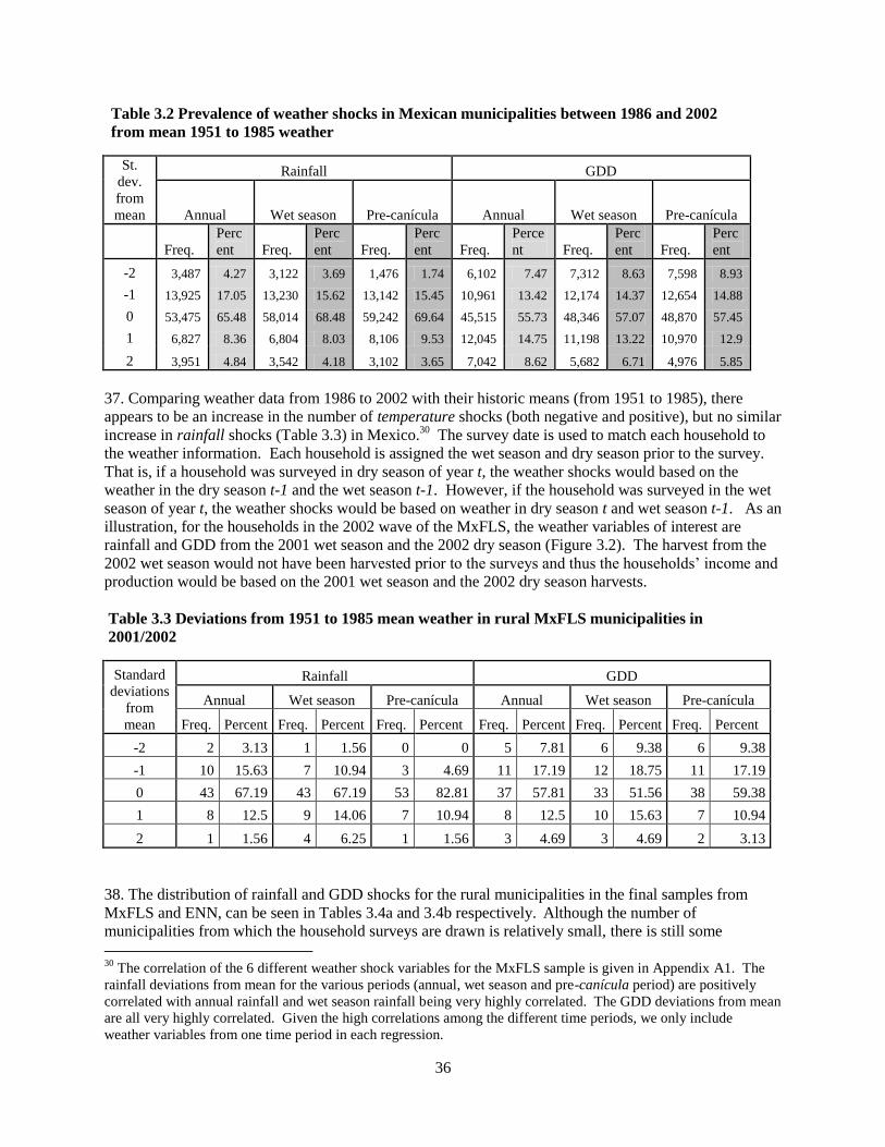
36

Table 3.2 Prevalence of weather shocks in Mexican municipalities between 1986 and 2002

from mean 1951 to 1985 weather

St.

dev.

from

mean

Rainfall GDD

Annual Wet season Pre-canícula Annual Wet season Pre-canícula

Freq.

Perc

ent Freq.

Perc

ent Freq.

Perc

ent Freq.

Perce

nt Freq.

Perc

ent Freq.

Perc

ent

-2 3,487 4.27 3,122 3.69 1,476 1.74 6,102 7.47 7,312 8.63 7,598 8.93

-1 13,925 17.05 13,230 15.62 13,142 15.45 10,961 13.42 12,174 14.37 12,654 14.88

0 53,475 65.48 58,014 68.48 59,242 69.64 45,515 55.73 48,346 57.07 48,870 57.45

1 6,827 8.36 6,804 8.03 8,106 9.53 12,045 14.75 11,198 13.22 10,970 12.9

2 3,951 4.84 3,542 4.18 3,102 3.65 7,042 8.62 5,682 6.71 4,976 5.85

37. Comparing weather data from 1986 to 2002 with their historic means (from 1951 to 1985), there

appears to be an increase in the number of temperature shocks (both negative and positive), but no similar

increase in rainfall shocks (Table 3.3) in Mexico.30

The survey date is used to match each household to

the weather information. Each household is assigned the wet season and dry season prior to the survey.

That is, if a household was surveyed in dry season of year t, the weather shocks would based on the

weather in the dry season t-1 and the wet season t-1. However, if the household was surveyed in the wet

season of year t, the weather shocks would be based on weather in dry season t and wet season t-1. As an

illustration, for the households in the 2002 wave of the MxFLS, the weather variables of interest are

rainfall and GDD from the 2001 wet season and the 2002 dry season (Figure 3.2). The harvest from the

2002 wet season would not have been harvested prior to the surveys and thus the households‘ income and

production would be based on the 2001 wet season and the 2002 dry season harvests.

Table 3.3 Deviations from 1951 to 1985 mean weather in rural MxFLS municipalities in

2001/2002

Standard

deviations

from

mean

Rainfall GDD

Annual Wet season Pre-canícula Annual Wet season Pre-canícula

Freq. Percent Freq. Percent Freq. Percent Freq. Percent Freq. Percent Freq. Percent

-2 2 3.13 1 1.56 0 0 5 7.81 6 9.38 6 9.38

-1 10 15.63 7 10.94 3 4.69 11 17.19 12 18.75 11 17.19

0 43 67.19 43 67.19 53 82.81 37 57.81 33 51.56 38 59.38

1 8 12.5 9 14.06 7 10.94 8 12.5 10 15.63 7 10.94

2 1 1.56 4 6.25 1 1.56 3 4.69 3 4.69 2 3.13

38. The distribution of rainfall and GDD shocks for the rural municipalities in the final samples from

MxFLS and ENN, can be seen in Tables 3.4a and 3.4b respectively. Although the number of

municipalities from which the household surveys are drawn is relatively small, there is still some

30

The correlation of the 6 different weather shock variables for the MxFLS sample is given in Appendix A1. The

rainfall deviations from mean for the various periods (annual, wet season and pre-canícula period) are positively

correlated with annual rainfall and wet season rainfall being very highly correlated. The GDD deviations from mean

are all very highly correlated. Given the high correlations among the different time periods, we only include

weather variables from one time period in each regression.

37

variability in the weather variables. There are municipalities that experienced positive and negative

rainfall as well as GDD events. As Table 3.4 shows, there are more GDD shocks than rainfall shocks in

the sample.

Table 3.4a Weather shocks in MxFLS sample

Standard

deviations

from

mean

Rainfall GDD

Annual Wet season Pre-canícula Annual Wet season Pre-canícula

Freq. % Freq. % Freq. % Freq. % Freq. % Freq. %

-2 10 4.63 6 2.67 8 3.54 13 6.02 13 5.78 14 6.19

-1 36 16.67 39 17.33 26 11.5 35 16.2 35 15.56 35 15.49

0 142 65.74 147 65.33 167 73.89 126 58.33 135 60.00 142 62.83

1 20 9.26 22 9.78 23 10.18 33 15.28 35 15.56 29 12.83

2 8 3.70 11 4.89 2 0.88 9 4.17 7 3.11 6 2.65

Note: Deviations from 1951 to 1985 mean weather in rural MxFLS municipalities for agricultural years prior to

household survey.

Table 3.4b Weather shocks in ENN sample

Standard

deviations

from

mean

Rainfall GDD

Annual Wet season Pre-canícula Annual Wet season Pre-canícula

Freq. % Freq. % Freq. % Freq. % Freq. % Freq. %

-2 3 1.67 6 3.33 14 7.78 9 5.00 8 4.44 7 3.89

-1 31 17.22 32 17.78 83 46.11 25 13.89 15 8.33 20 11.11

0 128 71.11 128 71.11 79 43.89 93 51.67 100 55.56 100 55.56

1 15 8.33 11 6.11 3 1.67 41 22.78 40 22.22 35 19.44

2 3 1.67 3 1.67 1 0.56 12 6.67 17 9.44 18 10.00

Note: Deviations from 1951 to 1985 mean weather in rural ENN municipalities for agricultural years prior to

household survey.

38

Table 3.4 Correlations between weather shock variables and average (1951-1985) weather

Dev

iati

on

in

ann

ual

rai

nfa

ll

fro

m m

ean

Dev

iati

on

in

wet

sea

son

rain

fall

fro

m m

ean

Dev

iati

on

in

pre

-can

ícu

la

rain

fall

fro

m m

ean

Dev

iati

on

in

ann

ual

GD

D

fro

m m

ean

Dev

iati

on

in

wet

sea

son

GD

D f

rom

mea

n

Dev

iati

on

in

pre

-can

ícu

la

GD

D f

rom

mea

n

Deviation in wet season rainfall from mean 0.953

Deviation in pre-canícula rainfall from mean 0.517 0.397

Deviation in annual GDD from mean -0.027 0.044 -0.059

Deviation in wet season GDD from mean -0.016 0.061 -0.060 0.965

Deviation in pre-canícula GDD from mean -0.016 0.082 -0.116 0.907 0.959

Average annual rainfall (1951-1985) -0.101 -0.230 0.086 -0.083 -0.084 -0.139

Average wet season rainfall (1951-1985) -0.087 -0.219 0.136 -0.106 -0.095 -0.157

Average pre-canicula rainfall (1951-1985) 0.004 -0.141 0.194 -0.103 -0.121 -0.194

Average annual GDD (1951-1985) -0.014 0.064 -0.242 0.032 0.068 0.193

Average wet season GDD (1951-1985) -0.053 0.046 -0.279 0.092 0.104 0.234

Average pre-canicula GDD (1951-1985) -0.028 0.018 -0.187 0.025 0.041 0.158

39. The original MxFLS localities, those chosen for the 2002 survey, come from 16 different Mexican

states and from all the different regions of the country. Although these states vary in the percentage of

land cultivated under rainfed technologies, in most at least 75% of the land is rainfed (Table 3.5). Also,

in most at least 50% of the land cultivated in the wet season is in corn and in all the area cultivated in the

wet season is greater than the area cultivated in the dry season. These figures suggest that it can be

expected that for an average rural household in the sample the income, as well as production for self

consumption, to be relatively highly dependent on the weather and especially on the weather during the

wet season. Also, given the relative importance of corn, the pre-canícula period is of interest.

39

Table 3.5 Agricultural production in Mexican states included in the MxFLS

Hectares cultivated

% of land in

corn % of land in beans

% of land in

sorghum

% of land in

other wet

season/ dry

season

hectares

% land

rainfed Region State

Dry

season

Wet

season

Dry

season

Wet

season

Dry

season

Wet

season

Dry

season

Wet

season

Dry

season

Wet

season

National production 2,167,069 13,758,639 31 59 11 12 13 13 45 15 6.35 82

North

Baja California Sur 16,722 28,987 12 41 11 11 2 8 74 41 1.73 27

Coahuila 44,874 281,365 3 27 1 6 9 47 87 20 6.27 66

Durango 57,155 691,738 12 42 16 30 17 6 55 22 12.10 80

Nuevo Leon 33,360 209,576 12 49 3 3 15 39 70 9 6.28 78

Sinaloa 418,177 588,288 63 39 13 4 3 44 21 13 1.41 54

Sonora 276,237 341,731 4 12 1 4 2 36 94 49 1.24 41

Center

Guanajuato 38,385 823,889 13 56 4 11 0 24 83 9 5.95 67

Jalisco 52,172 732,411 26 87 5 2 3 7 66 4 14.04 85

Estado de Mexico 42,074 544,033 25 81 7 2 7 0 61 17 12.93 89

Michoacán 86,904 668,846 18 79 2 1 28 13 52 7 7.70 78

Morelos 50,639 83,328 3 37 1 3 92 43 4 16 1.65 72

Puebla 39,153 709,046 41 73 13 9 2 3 45 15 18.11 88

Mexico

City Distrito Federal 2,924 12,297 4 42 1 2 11 0 84 55 4.21 94

South

Pacific Oaxaca 54,170 611,187 64 84 22 7 2 4 12 5 11.28 96

Gulf and

Caribbean

Veracruz 106,147 517,278 83 86 9 5 1 2 8 7 4.87 97

Yucatan 8,370 220,175 46 79 33 11 0 0 20 10 26.31 92

Source: NEGI. Censo Agricola, Ganadero y Forestal (2007).

Note: Regional assignations are taken from Conroy (2009)

40

40. Besides differing in the types of crops cultivated, the localities also differ in the availability of

services and programs. Table 3.6a summarizes some of the locality characteristics for the 2002 and 2005

MxFLS samples.31

The information is only available for those localities in the original sample. In 2005

there were households from 85 different localities since some of the households had moved to non-

MxFLS localities. In most of the original MxFLS localities there was access to primary education but

access to higher education was only readily accessible in a few localities. In many localities there were

health services available, as about 75% of the localities had a public health clinic, but not all had such

services locally. In the majority (about 75% in the 2002 sample and 99% in the 2005 sample), but not in

all, qualifying households were able to access Oportunidades.32

Table 3.6b shows some characteristics of

the ENN sample localities. Although on average 76% of the households in the localities have electricity,

only 27% have access to a sewage system.

Table 3.6a Select characteristics of localities in MxFLS sample

Characteristic of locality

Localities

with

information

in 2002

% of localities in

2002 with service

/ program

Localities

with

information

in 2005

% of localities

in 2005 with

service /

program

OPORTUNIDADES available 70 0.757 65 0.985

Primary school in locality 69 0.986 66 0.970

Secondary school in locality 70 0.343 66 0.364

Technical/trade school in locality 70 0.071 66 0.045

Public health clinic in locality 70 0.743 66 0.652

Note: Tabulated from MxFLS Community Survey Module. In the original survey households from 70 different

localities were surveyed. For the 2005 survey information from official sources was used as the primary source.

If there was no information from an official source, unofficial information was used. When two or more

official sources reported information and the information was conflicting, the variable was treated as a missing

value.

Table 3.6b Select characteristics of localities in ENN sample

Locality characteristic Mean Std. Dev.

Percentage of household with electricity 0.755

Percentage of household with running water 0.585

Percentage of household with a sewage system 0.265

Average household size 5.19 0.89

Altitude from sea level (m) 1168 867

Note: Based on 547 rural localities where there are households with children under 3 years of age in the Encuesta

Nacional de Nutricion.

31

The information is more complete, although maybe more unreliable, for the 2002 sample. In 2005 information

was sought from both official and unofficial sources. Information from official sources was used as the primary

source of information and if no official information was available then the unofficial information was used instead.

If more than one official source of information was used, and the information was conflicting, i.e. one source

responding yes to the presence of a secondary school in the locality and the other responding no, the variable was

coded as missing. Given this fact, in 2005 there are more observations with missing information than in 2002. 32

Oportunidades, originally named PROGRESA, is a conditional cash transfer (CCT) program aimed to alleviate

current poverty through monetary and in-kind benefits.

41

3.5 Results

41. The results from the analyses on the impacts of rainfall and GDD shocks on household consumption

and on the health outcomes of children are presented next. To examine whether or not weather shocks

impact household consumption, equation (3.1) is estimated. Consumption is measured by the logarithm

of per capita expenditures on all non-health related items. Health spending is subtracted from the total

expenditures since most health spending follows illness and thus is not welfare improving (Thomas et al.,

2010). The impact of weather on food expenditures given that households may spend on different

spending categories after weather shocks is also examined. The average share of food expenditures in the

sample is 41% of total expenditures (without considering health expenditures). Included in the

expenditures are the estimated value of goods consumed from own production and the value of goods

received as gifts.33

That is, the expenditure measure used reflects wellbeing after taking into account any

self-production or any coping mechanisms used by households to smooth consumption (such as selling

assets, help from friends and relatives, or benefits from government programs). The extent to which these

impacts have long-run implications on the poverty status of the future welfare and poverty status of the

household is beyond the scope of this study.

42. Besides the weather shock variables the variables include capture household composition (number of

children in the household, number of adult males in the household, number of adult females in the

household), characteristics of the household head (years of schooling of the household head, gender of the

household head, and the age of the household head), an asset index,34

and the characteristics of the

housing unit (presence of a kitchen, access to tapped water indoors, presence of a toilet, access to piped

sewage or septic tank, electricity, and flooring material). These variables are all thought to explain

expenditures. To control for the agro-climatic conditions and other time invariant characteristics locality

fixed effects are introduced. To account for any systematic change between the two survey periods, the

analysis controls for the survey wave. Furthermore to account for the potentially different amount of

resources available depending on the season in which the household responded to the survey, season

indicator variable is introduced. Appendix A2 gives the descriptive statistics of the variables used in the

analyses.

3.5.1 Impacts of climatic variability on expenditures

43. Six different specifications were run with different measures of welfare and different measures of

weather shocks based on equation (3.1). Given differences in the average climatic conditions in the

North, and the Centre and South regions of the country besides including all rural households, the sample

is limited to only those households in the North and to only those households in the Centre and South.

The first set of specifications uses the (ln) per capita expenditures on all non-health items and the second

set uses the (ln) per capita expenditures on food as the dependent variable. For each welfare measure 3

different specifications are estimated. The first uses weather shocks in the prior agricultural year‘s annual

rainfall and annual GDD. The second uses weather shocks in the prior wet season and the third in the

prior pre-canícula period. Fixed effects are first introduced at the state level and then at the locality level.

33

Given the way in which the expenditure survey was administered, it is not possible to separate the value of

consumption from own production from the value of goods received as gifts. For about 7% of the rural households

more than 50% of their food comes from non-purchased sources. On average for a rural household about 7% of all

food comes from non-purchased sources. 34

The asset index is based on the principal factor analysis of how many parcels of land the household owns, whether

or not the household owns their residence, another house, bicycle, motor vehicle, an electric device, a washing

machine or a stove, a domestic appliance, machinery or a tractor, bulls or cows, horses or mules, pigs or goats, or

poultry.

42

44. The results were relatively insensitive to which geographic fixed effects are used and the coefficient

estimates for the weather shock variables were reported with locality fixed effects.35

45. In terms of rainfall, on average a rural Mexican household spends more on non-health items after

negative annual rainfall shocks and more on food after a positive annual rainfall shock (Table 3.7).

Namely, if the prior agricultural year was at least one standard deviation drier than the 1951-1985

average, the per capita expenditures are 14 percent higher and per capita expenditures on food are 18

percent greater when the annual rainfall is at least one standard deviation more than the 1951 - 1985

average.

35

Appendix A3 shows the complete set of coefficient estimates for all rural households using fixed effects at the

state and at the locality level.

43

Table 3.7 Weather shocks and expenditures per capita

Variable

All rural households Central and South North

Annual Wet season

Pre-

canícula Annual Wet season

Pre-

canícula Annual Wet season

Pre-

canícula

Dependent variable: Per capita expenditures (ln) in non-health items

Negative rainfall shock 0.141* 0.065 -0.000 0.246*** 0.110 -0.075 0.057 -0.030 0.121

(0.082) (0.096) (0.080) (0.090) (0.112) (0.103) (0.143) (0.154) (0.189)

Positive rainfall shock 0.068 -0.008 -0.014 0.247** 0.109 -0.026 -0.024 -0.086 0.026

(0.087) (0.072) (0.086) (0.100) (0.095) (0.104) (0.109) (0.094) (0.133)

Negative GDD shock -0.023 0.022 -0.013 -0.039 0.183 0.205** 0.076 -0.057 -0.328***

(0.093) (0.131) (0.129) (0.127) (0.111) (0.095) (0.132) (0.209) (0.107)

Positive GDD shock 0.027 0.183** 0.081 -0.127 0.142 0.075 0.032 0.149 0.092

(0.092) (0.082) (0.115) (0.115) (0.090) (0.126) (0.151) (0.134) (0.180)

Number of observations 4,929 4,950 4,951 2,624 2,641 2,642 2,305 2,309 2,309

Dependent variable: Per capita expenditures (ln) in food

Negative rainfall shock -0.085 0.057 -0.028 -0.070 0.126 -0.103 -0.111 -0.150 0.131

(0.109) (0.111) (0.148) (0.185) (0.167) (0.192) (0.103) (0.111) (0.246)

Positive rainfall shock 0.179* 0.131 0.036 0.404** 0.322 0.030 0.085 0.019 0.062

(0.107) (0.119) (0.119) (0.184) (0.209) (0.163) (0.102) (0.099) (0.155)

Negative GDD shock -0.249 -0.041 0.221 -0.045 0.329 0.396* -0.369*** -0.276** 0.032

(0.162) (0.184) (0.159) (0.300) (0.231) (0.198) (0.122) (0.129) (0.157)

Positive GDD shock 0.150 -0.062 -0.110 0.022 -0.281 -0.020 0.156* 0.010 -0.193

(0.099) (0.140) (0.154) (0.164) (0.244) (0.221) (0.090) (0.166) (0.203)

Number of observations 4,929 4,950 4,951 2,624 2,641 2,642 2,305 2,309 2,309

Source: Skoufias et al. (2011b)

Note: Robust standard errors in parentheses, clustered by locality, and *** p<0.01, ** p<0.05, * p<0.1. Calculated using MxFLS rounds 1 and 2 with locality level

fixed effects. A negative weather shock identifies those municipalities which in the previous agricultural year (or wet season or pre-canícula period) had at least 1

standard deviation less rain (or GDD) than in an average year. Similarly, a positive weather shock identifies those municipalities which in the previous agricultural

year (or wet season or pre-canícula period) had at least 1 standard deviation more rain (or GDD) than in an average year. Other independent variables included are:

household composition (number of children in the household, number of adult males in the household, number of adult females in the household), characteristics of

the household head (sex, age and education), assets ( index based on how many parcels of land the household owns, whether or not the household owns their

residence, another house, bicycle, motor vehicle, an electric device, a washing machine or a stove, a domestic appliance, machinery or a tractor, bulls or cows,

horses or mules, pigs or goats, or poultry), characteristics of the housing unit (presence of a kitchen, access to tapped water indoors, toilet, access to piped sewage

or septic tank, electricity, floor type).

44

46. The results are quite different when equation (3.1) is estimated separately for each of the two

regions—North and Center/South.36

In the North, the more arid region of the country and with a higher

percentage of irrigated land, a negative rainfall shock has no impacts on expenditures. However, for the

Centre/South region both negative and positive rainfall shocks are associated with higher expenditures on

non-health items (by 25%) and positive rainfall shocks are also associated with higher expenditures on

food (Table 3.7). The results suggest that in the Centre/South regions both types of rainfall shocks are

welfare improving. 37

47. The results in terms of temperature indicate that the warmer than average wet seasons are associated

with 18 percent higher expenditures per capita (Table 3.7). That is, on average, for the sample of

Mexican households, warmer weather is in fact welfare improving. However, when the sample is

separated in two—North and Center/South—positive wet season GDD shocks no longer are statistically

significantly welfare improving.38

In addition, negative GDD shocks during the pre-canícula period are

associated with higher expenditures on all non-health items as well as higher expenditures on food in the

Central/South sample and lower non-health expenditures in the North sample. In the North, food

expenditures are also lower after a negative GDD shock during the prior agricultural year (37% lower)

and during the prior wet season (28% lower). These results reflect Galindo‘s (2009) findings of variable

impacts on agricultural production from changes in temperature by region and by the type of crop

cultivated.

48. It is interesting to note that in the sample, on average, unusual weather (that is, weather that is at least

one standard deviation from the mean) is never associated with lower welfare, with the exception of

negative GDD shocks in the North. That is, even if the shocks do have a negative impact on agricultural

production, the households do not see a reduction in their expenditures. This suggests that households are

either able to protect themselves ex-ante by changing their agricultural practices in response to the

weather shocks, or in the case of reduced agricultural revenue, that households are able ex-post to keep

expenditures (and welfare) from deteriorating by drawing down on their assets, or receiving help from

formal and informal safety networks, such as relatives or social programs, or accessing credit. While these

types of responses used by the households are deserving of deeper analysis they are not within the scope

of this study.

3.5.2 Heterogeneity of impacts

49. The average impacts may mask difference in response between types of households to weather

shocks. The difference in welfare levels by the sex and by the educational attainment of the household

head was examined by estimating equation (3.2). In general, a household headed by a female is never

worse off because of a weather shock than a household headed by a male. In fact, if there is a positive

annual or pre-canícula period rainfall shock female headed households have a higher per capita

expenditure than male headed households by 16 percent and 25 percent, respectively (Table 3.8a).

Furthermore, with positive annual rainfall shocks food expenditures per capita are 28 percent higher in

36

The North includes the states of Baja California, Baja California Sur, Chihuahua, Coahuila, Durango, Nuevo

Leon, Sinaloa, Sonora, Tamaulipas, and Zacatecas. All the other states are part of Center/South region. 37

It is possible that the higher expenditure may be a consequence of the higher local prices faced by households

rather than due to an increase in the quantity of goods consumed. We tried to shed some light on this issue, by

regressing the average price (based on one to three stores) of a food item on the weather shocks controlling for state

fixed effects. We found rather mixed results since for those municipalities in the Center/South of the country, the

prices of five items are positively correlated with a positive rainfall shock (potato, lemon, chili, pork, and white

bread) and four items are negatively correlated (tomato, apple, beef, and whole fish). 38

The coefficient estimate is positive for both samples

45

female headed households than in male headed ones (Table 3.8b). Similarly a female headed household

in a municipality with a positive pre-canícula GDD shock has, on average, 44 percent higher per capita

expenditures on food than male headed households.

50. Examining the households by the two regions—North, Center/South—separately, differences between

female and male headed households are found. Female headed households in the central and southern

parts of the country have higher expenditures after a positive rainfall shock than the region‘s male headed

households. Both non-health expenditures as well as food expenditures are between 28 percent and 42

percent higher, respectively. In contrast, female headed households in the North have 30 percent lower

non-health expenditures than male headed households after a positive wet season rainfall shock.

However, female headed households in the North are not statistically significantly different from male

headed households in terms of food expenditures, suggesting that food expenditures are protected from

the effects of the positive rainfall shock. Also, it is the northern female headed households who are

positively affected by a positive pre-canícula GDD shock.

51. The education level of the household head also matters (Table 3.9a and 3.9b). On average, for some

weather shocks, households where the head has not completed primary school have lower non-health and

food expenditures per capita than households where the head has completed primary school. In terms of

rainfall, on average households with less educated heads have 16% lower non-health expenditures after a

positive pre-canícula rainfall shock, and 29% lower food expenditures after a negative pre-canícula

rainfall shock. After separate analyses for the two regions, while statistically significant differences in the

impacts of rainfall shocks on non-health expenditures are not found, regional differences on food

expenditures are. In the northern states, households with less educated heads have 38 percent higher

expenditures on food and 51 percent lower expenditures on food than households where the head has

completed primary school after a negative rainfalls shock during the prior year and the prior pre-canícula,

respectively.

52. Less educated households are more affected by GDD shocks than rainfall shocks and these differential

effects are observed only in food expenditures. The less educated households have on average 14% lower

food expenditures after a negative annual GDD shock and 34% lower food expenditures after a positive

annual GDD shock than household where the household head has completed primary schooling.

Separating the household regionally, no differential impacts either in the Center/South grouping or in the

North after a negative GDD shock are observed.39

However, large negative differentials in the North after

positive GDD shocks are observed, regardless of the timing of the shock during the agricultural year (i.e.,

during the wet season or during the pre-canícula period). The negative differential suggests that

households with less educated heads are less able to modify their agricultural practices to take advantage

of more advantageous weather or to counter negative impacts of unfavorable weather. Another possibility

is that households with less educated heads cannot access other mechanisms to offset negative effects of

weather shocks on welfare. The only exception is a negative rainfall shock in the North when the less

educated households do not have lower food expenditures whereas the more educated households do.

This peculiar differential effect could be explained if crop choice is determined by education.

39

The coefficient estimates for negative annual GDD shocks are negative in both regions, but not statistically

significant.

46

Table 3.8a Per capita expenditures (ln) on non-health items

Variables

All rural households Central and South North

Annual Wet season

Pre-

canícula Annual Wet season

Pre-

canícula Annual Wet season

Pre-

canícula

HH head is female 0.007 0.011 -0.084 -0.095 -0.114 -0.158 0.106 0.151 -0.001

(0.070) (0.083) (0.083) (0.113) (0.111) (0.122) (0.079) (0.109) (0.108)

Negative rainfall shock 0.153* 0.066 -0.010 0.269** 0.130 -0.107 0.043 -0.051 0.118

(0.084) (0.101) (0.080) (0.103) (0.130) (0.104) (0.140) (0.153) (0.191)

... X female HH head -0.089 -0.018 0.049 -0.123 -0.091 0.153 0.211 0.209 0.000

(0.207) (0.236) (0.232) (0.258) (0.329) (0.243) (0.191) (0.176) (0.000)

Positive rainfall shock 0.032 -0.007 -0.065 0.170 0.042 -0.118 -0.013 -0.021 0.043

(0.088) (0.067) (0.086) (0.104) (0.089) (0.099) (0.107) (0.087) (0.150)

... X female HH head 0.163* -0.004 0.250* 0.351** 0.284** 0.423** -0.042 -0.303* -0.083

(0.095) (0.120) (0.128) (0.135) (0.127) (0.160) (0.117) (0.167) (0.159)

Negative GDD shock 0.016 0.043 -0.016 -0.016 0.180* 0.199* 0.103 -0.064 -0.346***

(0.096) (0.132) (0.126) (0.123) (0.106) (0.099) (0.146) (0.217) (0.112)

... X female HH head -0.153 -0.092 -0.020 -0.093 -0.051 -0.076 -0.108 0.014 0.102

(0.112) (0.115) (0.123) (0.166) (0.163) (0.169) (0.135) (0.123) (0.161)

Positive GDD shock 0.043 0.197** 0.057 -0.134 0.126 0.053 0.064 0.179 0.068

(0.095) (0.090) (0.115) (0.123) (0.117) (0.131) (0.156) (0.144) (0.180)

... X female HH head -0.078 -0.077 0.132 0.061 0.056 0.062 -0.189 -0.166 0.148

(0.140) (0.163) (0.138) (0.169) (0.238) (0.281) (0.208) (0.212) (0.114)

Source: Skoufias et al. (2011b)

Note: Robust standard errors in parentheses, clustered by locality, and *** p<0.01, ** p<0.05, * p<0.1. Calculated using MxFLS rounds 1 and 2 with locality level

fixed effects. A negative weather shock identifies those municipalities which in the previous agricultural year (or wet season or pre-canícula period) had at least 1

standard deviation less rain (or GDD) than in an average year. Similarly, a positive weather shock identifies those municipalities which in the previous agricultural

year (or wet season or pre-canícula period) had at least 1 standard deviation more rain (or GDD) than in an average year. Other independent variables included are:

household composition (number of children in the household, number of adult males in the household, number of adult females in the household), characteristics of

the household head (sex, age and education), assets ( index based on how many parcels of land the household owns, whether or not the household owns their

residence, another house, bicycle, motor vehicle, an electric device, a washing machine or a stove, a domestic appliance, machinery or a tractor, bulls or cows,

horses or mules, pigs or goats, or poultry), characteristics of the housing unit (presence of a kitchen, access to tapped water indoors, toilet, access to piped sewage

or septic tank, electricity, floor type).

47

Table 3.8b Per capita expenditures (ln) on food

Variables

All rural households Central and South North

Annual Wet season

Pre-

canícula Annual Wet season

Pre-

canícula Annual Wet season

Pre-

canícula

HH head is female -0.042 -0.080 -0.082 -0.060 -0.067 -0.063 -0.019 -0.098 -0.105

(0.129) (0.126) (0.109) (0.199) (0.172) (0.153) (0.165) (0.170) (0.147)

Negative rainfall shock -0.080 0.032 -0.024 -0.081 0.102 -0.102 -0.066 -0.174 0.120

(0.106) (0.117) (0.148) (0.183) (0.175) (0.195) (0.111) (0.117) (0.246)

... X female HH head -0.059 0.190 -0.061 0.060 0.136 -0.015 -0.540 0.290 0.000

(0.190) (0.187) (0.223) (0.218) (0.240) (0.248) (0.603) (0.191) (0.000)

Positive rainfall shock 0.122 0.087 -0.015 0.320 0.235 -0.036 0.055 0.019 0.055

(0.115) (0.130) (0.119) (0.206) (0.232) (0.163) (0.097) (0.120) (0.157)

... X female HH head 0.279** 0.208 0.238 0.395* 0.384* 0.288 0.123 0.012 0.079

(0.121) (0.141) (0.161) (0.231) (0.195) (0.215) (0.121) (0.204) (0.170)

Negative GDD shock -0.218 -0.021 0.218 0.005 0.352 0.400** -0.378*** -0.276* 0.017

(0.153) (0.174) (0.151) (0.288) (0.213) (0.194) (0.134) (0.143) (0.166)

... X female HH head -0.121 -0.083 -0.006 -0.166 -0.154 -0.085 -0.003 0.079 0.110

(0.154) (0.134) (0.154) (0.232) (0.179) (0.222) (0.175) (0.159) (0.157)

Positive GDD shock 0.103 -0.107 -0.189 -0.018 -0.303 -0.080 0.118 -0.056 -0.277

(0.116) (0.149) (0.168) (0.211) (0.254) (0.237) (0.092) (0.187) (0.220)

... X female HH head 0.244 0.244 0.438** 0.238 0.128 0.248 0.243 0.371 0.567**

(0.178) (0.185) (0.171) (0.271) (0.198) (0.217) (0.249) (0.257) (0.225)

Number of observations 4,929 4,950 4,951 2,624 2,641 2,642 2,305 2,309 2,309

Source: Skoufias et al. (2011b) Note: Robust standard errors in parentheses, clustered by locality, and *** p<0.01, ** p<0.05, * p<0.1. Calculated using MxFLS rounds 1 and 2 with locality level

fixed effects. A negative weather shock identifies those municipalities which in the previous agricultural year (or wet season or pre-canícula period) had at least 1

standard deviation less rain (or GDD) than in an average year. Similarly, a positive weather shock identifies those municipalities which in the previous agricultural

year (or wet season or pre-canícula period) had at least 1 standard deviation more rain (or GDD) than in an average year. Other independent variables included are:

household composition (number of children in the household, number of adult males in the household, number of adult females in the household), characteristics of

the household head (sex, age and education), assets ( index based on how many parcels of land the household owns, whether or not the household owns their

residence, another house, bicycle, motor vehicle, an electric device, a washing machine or a stove, a domestic appliance, machinery or a tractor, bulls or cows,

horses or mules, pigs or goats, or poultry), characteristics of the housing unit (presence of a kitchen, access to tapped water indoors, toilet, access to piped sewage

or septic tank, electricity, floor type).

48

Table 3.9a Per capita (ln) expenditure on non-health items

Variables

All rural households Central and South North

Annual Wet season

Pre-

canícula Annual Wet season

Pre-

canícula Annual Wet season

Pre-

canícula

HH head has not completed

primary school

-0.154** -0.180*** -0.168** -0.264*** -0.348*** -0.303*** -0.089 -0.037 -0.087

(0.064) (0.067) (0.066) (0.078) (0.083) (0.088) (0.107) (0.108) (0.093)

Negative rainfall shock 0.184* 0.061 0.079 0.233* 0.023 -0.107 0.085 0.023 0.277

(0.100) (0.123) (0.097) (0.137) (0.176) (0.108) (0.160) (0.157) (0.194)

... X no primary school -0.075 0.006 -0.127 0.017 0.131 0.050 -0.051 -0.099 -0.365

(0.136) (0.149) (0.119) (0.196) (0.256) (0.122) (0.140) (0.116) (0.221)

Positive rainfall shock 0.090 0.012 0.090 0.282*** 0.096 0.020 -0.011 -0.026 0.117

(0.091) (0.075) (0.086) (0.099) (0.101) (0.098) (0.118) (0.095) (0.138)

... X no primary school -0.038 -0.036 -0.159** -0.050 0.030 -0.062 -0.025 -0.107 -0.154

(0.075) (0.074) (0.079) (0.081) (0.086) (0.096) (0.108) (0.118) (0.122)

Negative GDD shock 0.001 0.021 -0.041 -0.074 0.095 0.114 0.106 -0.004 -0.316**

(0.100) (0.135) (0.124) (0.124) (0.122) (0.106) (0.155) (0.216) (0.129)

... X no primary school -0.042 0.001 0.039 0.055 0.160 0.128 -0.054 -0.106 -0.006

(0.072) (0.076) (0.072) (0.084) (0.095) (0.091) (0.126) (0.141) (0.142)

Positive GDD shock 0.032 0.175* 0.078 -0.074 0.102 0.041 0.061 0.209 0.139

(0.094) (0.092) (0.109) (0.129) (0.125) (0.190) (0.153) (0.144) (0.150)

... X no primary school -0.007 0.016 0.007 -0.076 0.053 0.062 -0.054 -0.119 -0.096

(0.086) (0.104) (0.094) (0.102) (0.200) (0.202) (0.124) (0.114) (0.113)

Source: Skoufias et al. (2011b)

Note: Robust standard errors in parentheses, clustered by locality, and *** p<0.01, ** p<0.05, * p<0.1. Calculated using MxFLS rounds 1 and 2 with locality level

fixed effects. A negative weather shock identifies those municipalities which in the previous agricultural year (or wet season or pre-canícula period) had at least 1

standard deviation less rain (or GDD) than in an average year. Similarly, a positive weather shock identifies those municipalities which in the previous agricultural

year (or wet season or pre-canícula period) had at least 1 standard deviation more rain (or GDD) than in an average year. Other independent variables included are:

household composition (number of children in the household, number of adult males in the household, number of adult females in the household), characteristics of

the household head (sex, age and education), assets ( index based on how many parcels of land the household owns, whether or not the household owns their

residence, another house, bicycle, motor vehicle, an electric device, a washing machine or a stove, a domestic appliance, machinery or a tractor, bulls or cows,

horses or mules, pigs or goats, or poultry), characteristics of the housing unit (presence of a kitchen, access to tapped water indoors, toilet, access to piped sewage

or septic tank, electricity, floor type).

49

Table 3.9b Per capita (ln) expenditure on food

Variables All rural households Central and South North

Annual Wet season

Pre-

canícula Annual Wet season

Pre-

canícula Annual Wet season

Pre-

canícula

HH has not completed

primary school

0.080 0.052 0.069 -0.025 -0.103 -0.039 0.159* 0.182 0.119

(0.064) (0.081) (0.071) (0.089) (0.098) (0.100) (0.081) (0.117) (0.097)

Negative rainfall shock -0.153 -0.002 0.151 -0.111 0.005 0.000 -0.317** -0.161 0.362*

(0.127) (0.147) (0.136) (0.185) (0.198) (0.197) (0.151) (0.150) (0.192)

... X no primary school 0.118 0.100 -0.285* 0.063 0.174 -0.146 0.376* 0.012 -0.509**

(0.180) (0.185) (0.157) (0.226) (0.259) (0.196) (0.194) (0.171) (0.199)

Positive rainfall shock 0.210* 0.156 0.132 0.406* 0.295 0.097 0.160 0.103 0.099

(0.119) (0.136) (0.149) (0.240) (0.243) (0.210) (0.117) (0.115) (0.155)

... X no primary school -0.035 -0.046 -0.151 -0.002 0.046 -0.089 -0.120 -0.159 -0.057

(0.101) (0.111) (0.120) (0.184) (0.175) (0.166) (0.092) (0.123) (0.103)

Negative GDD shock -0.169 0.021 0.272* -0.023 0.342 0.398* -0.273** -0.227* 0.089

(0.173) (0.191) (0.157) (0.311) (0.246) (0.206) (0.125) (0.126) (0.167)

... X no primary school -0.135* -0.100 -0.083 -0.036 0.008 -0.013 -0.142 -0.085 -0.068

(0.080) (0.086) (0.085) (0.097) (0.117) (0.117) (0.106) (0.116) (0.125)

Positive GDD shock 0.356*** 0.041 -0.033 0.137 -0.396 -0.220 0.427*** 0.259 0.020

(0.092) (0.144) (0.162) (0.153) (0.316) (0.384) (0.103) (0.157) (0.167)

... X no primary school -0.344*** -0.196 -0.152 -0.168 0.189 0.338 -0.531*** -0.469** -0.452*

(0.103) (0.155) (0.192) (0.170) (0.247) (0.325) (0.135) (0.172) (0.235)

Number of observations 4,929 4,950 4,951 2,624 2,641 2,642 2,305 2,309 2,309

Source: Skoufias et al. (2011b)

Note: Robust standard errors in parentheses, clustered by locality, and *** p<0.01, ** p<0.05, * p<0.1. Calculated using MxFLS rounds 1 and 2 with locality level

fixed effects. A negative weather shock identifies those municipalities which in the previous agricultural year (or wet season or pre-canícula period) had at least 1

standard deviation less rain (or GDD) than in an average year. Similarly, a positive weather shock identifies those municipalities which in the previous agricultural

year (or wet season or pre-canícula period) had at least 1 standard deviation more rain (or GDD) than in an average year. Other independent variables included

are: household composition (number of children in the household, number of adult males in the household, number of adult females in the household),

characteristics of the household head (sex, age and education), assets ( index based on how many parcels of land the household owns, whether or not the household

owns their residence, another house, bicycle, motor vehicle, an electric device, a washing machine or a stove, a domestic appliance, machinery or a tractor, bulls or

cows, horses or mules, pigs or goats, or poultry), characteristics of the housing unit (presence of a kitchen, access to tapped water indoors, toilet, access to piped

sewage or septic tank, electricity, floor type).

50

3.5.3 Impacts of climatic variability on child health

53. To analyze the impacts of weather on health outcomes the study focuses on children 36 months

or younger living in rural areas. This is the age group most likely to suffer negative health

outcomes and any impacts potentially have long term consequences. Between the ages of zero and

three the growth rates are faster than at any other point and thus any delays have a greater

probability of affecting overall growth (Martorell, 1999). Shrimpton et al. (2001) find that in

developing countries although the children when born are on average at the mean of standardized

height-for-age there is a sharp decline in the height-for-age from ages 0 months to 24 months and no

subsequent catching up in the first 5 year of life.

54. Furthermore, Martorell et al. (2010) find evidence that weight gain the first 2 years of life had a

strong impact on schooling outcomes whereas weight gain between 2 years and 4 years of life had a

weaker impact. Alderman (2010) emphasizes the fact that weather caused nutritional shocks

experienced in the first years of life have lasting impacts on productivity even if the household is

able to later on overcome poverty. Victora et al. (2008) find in their meta-analysis that height-for-

age and weight-for-age are strong predictors of school achievement and that stunting between 12

and 36 months of age is associated with poorer cognitive development.

55. The impacts of weather on child outcomes was also estimated. The standardized height-for-age

z-score for children 36-months or younger were used as the measure of health.40

Unlike weight-for-

age, height-for-age is not as sensitive to very short-term and immediate scarcities or illness, but

would capture more chronic conditions.41

Given that all the data were collected during the 1999 dry

season, the year and season terms drop out. Given that the weather data are at the municipal level,

state level fixed effects were used to control for the time invariant characteristics, such as the agro-

climatic conditions at the state level.

56. Besides the measures of weather shocks, other information was included on:

household composition (the number of children, the number of adult males, and the number of

adult females);

on mother‘s characteristics (mother‘s education, height, and whether she speaks an indigenous

language);

information about the child (gender, if the child has an older sibling who was born alive within

2 years of the child‘s birth, multiple birth, the birth order of the child, whether the child was

characterized as very small at birth, and the age of the child at the time anthropometric

measurement was taken);

an asset index; 42

housing characteristics (presence of indoor toilet, tap water, type of floor);

and information about the child‘s locality (altitude) as regressors in the analyses. 43

40

The study used, WHO Anthro for personal computers, version 3, 2009: Software for assessing growth and

development of the world's children. Geneva: WHO, 2009 (http://www.who.int/childgrowth/software/en/ ) for

calculating the standardized height-for-age scores. 41

The measure does not capture any differences in mortality from unusual weather. 42

The asset index is based on the principal factor analysis of the household‘s ownership of a radio, a

television, a VCR, a telephone, a computer, a refrigerator, a washing machine, a stove, a heater, and motor

vehicle. 43

Only when analyzing the effects by participation in a nutritional program, we also include nutritional

program participation as a regressor.

51

57. The variables used in the analyses are described in Table 3.10. Given the differences in the

average climate in the North and in the Centre/South regions, the children in each region are

analyzed separately.

58. There are 1,995 rural children less than 36 months in the ENN dataset. The sample consisted of

only 1,540 children.44

The study only included those children whose mother has not moved in the

past year to ensure that the weather shocks match what the child experienced. Of the excluded

children, there are 138 children with missing height information and 91 children with improbable z-

scores,45

suggesting data entry errors. The other excluded children have incomplete information on

the covariates. The children measured (and with probable z-scores) are statistically significantly

older than those who are not measured. This poses a problem given that those children who were

not measured are different, and they may be systematically different in other characteristics besides

age as well.46

Furthermore, since only a few children (less than 2 percent of the sample)

experienced a positive pre-canícula rainfall shock, the coefficient estimates for positive pre-

canícula rainfall should be interpreted with caution (Table 3.11).

59. Bearing these caveats in mind, Table 3.12 summarizes the average relationship between weather

shocks and height-for-age. The full results for the specification are included in Appendix A4. A

positive rainfall shock is associated with lower height-for-age scores. This is true for both a

positive annual and a positive wet season rainfall shocks. The coefficient estimate of around 0.5

points is non-trivial given that a z-score of -2 is indicative of stunting and the average height-for-

age z-score for the children in the sample is -1.09.47

The earlier results based on the MxFLS

consumption data suggest that there is no correlation between a positive rainfall shock and non-

health expenditures, and that households spend more on food. Yet, the height of children under

three years of age is negatively affected after such a shock. Together, these results suggest that

direct environmental effects are important and that an analysis of the impacts of weather shocks at

the household level has serious limitations in terms of capturing the impacts of these shocks on

certain individuals in the household.

60. The negative impacts of a positive rainfall shock during the prior agricultural year or wet season

are consistent in both of the regional subsamples (Table 3.12). The biggest impact is from a

positive rainfall shock during the wet season in the North. Children who experienced such a shock

are 0.7 points shorter than children who experienced an average amount of rain. Negative rainfall

shocks appear to have different impacts in the Centre/South regions than in the North. Children

living in the Center/South region are taller if the prior agricultural year or wet season was at least

one standard deviation drier than average. In the North, however, children are shorter after such a

shock.

61. Not all children experience the same kind of health outcomes from weather shocks. Tables

3.13, 3.14, and 3.15 present the results between weather shocks and sex of the child, the mother‘s

educational level, and the household‘s participation in a supplemental nutrition program,

respectively.

44

This is the pre-canícula sample without nutritional supplement program variables and access to health care

included as explanatory variables. 45

That is, their height-for-age z-scores are less than -6 or more than 6. 46

If those who are not measured are more likely to be sick (and some of these illness are due to the weather),

then the coefficient estimates of the weather shock variables is likely to provide a lower bound of the impact

of the weather shock. 47

The average does include the 144 children who lived in a locality where the rainfall was at least one

standard deviation more than on average. However, excluding these children the average z-score does not

change significantly and is -1.08.

52

Table 3.10 Characteristics of rural children

Variable All Center/South North

Mean

Std.

Dev. Mean

Std.

Dev. Mean

Std.

Dev.

Number of adult males in hh 1.375 0.942 1.349 0.857 1.434 1.114

Number of adult females in hh 1.502 0.912 1.475 0.799 1.566 1.132

Number of children (16 yrs or younger) in hh 3.449 1.893 3.693 2.000 2.876 1.464

Mother's height 148 23 146 22 152 24

Mother speaks an indigenous language 0.164 0.198 0.085

Education mother: has not completed primary 0.456 0.526 0.293

Sex 0.517 0.518 0.514

Birth order 3.372 2.480 3.651 2.679 2.720 1.775

Multiple birth 0.017 0.017 0.017

Categorized as very small at birth 0.071 0.071 0.069

Has an older sibling less than 2 years apart 0.184 0.195 0.158

Age: 6 months to 12 months 0.180 0.174 0.193

Age: 12 months to 24 months 0.333 0.332 0.336

Age: 24 months to 36 months 0.329 0.338 0.306

Altitude of locality (in km) 1.192 0.892 1.305 0.870 0.929 0.888

Household asset score -0.305 0.719 -0.487 0.652 0.120 0.688

Floor of dirt 0.338 0.383 0.234

No tap water to kitchen or bath 0.866 0.908 0.766

No proper indoor toilet 0.745 0.758 0.716

Observations 1540 1079 461

Source: Data come from the Encuesta Nacional de Salud.

53

Table 3.11 Number of observations for different sub-populations and types of weather shocks

Sub population

Rainfall GDD

Negative shock Positive shock Negative shock Positive shock

Annual Wet

season

Pre-

canícu-

la

Annual Wet

season

Pre-

canícu-

la

Annual Wet

season

Pre-

canícu-

la

Annual Wet

season

Pre-

canícu-

la

Boys 117 128 417 59 50 7 102 57 75 238 241 227

Girls 106 127 444 85 73 14 104 73 81 238 274 249

Mother has completed

primary school 112 124 443 79 77 9 100 62 75 267 301 262

Mother hasn‘t completed

primary school 111 131 418 65 46 12 106 68 81 209 214 214

Not in a nutritional

program 107 145 463 90 79 19 85 54 68 254 270 272

In a nutritional program 116 110 398 54 44 2 121 76 88 220 245 204

Total number of

observations 1,536 1,536 1,540 1,536 1,536 1,540 1,536 1,536 1,540 1,536 1,536 1,540

Note: Based on ENN and includes all children under 36 months and with non-missing information on all covariates.

54

Table 3.12 Impact of weather on child's height-for-age

Variables All Centre/South North

Annual

Wet

season

Pre-

canícula Annual

Wet

season

Pre-

canícula Annual

Wet

season

Pre-

canícula

Negative rainfall shock 0.185 0.246 -0.025 0.384* 0.479** 0.127 -0.265 -0.294** -0.371*

(0.150) (0.166) (0.128) (0.204) (0.228) (0.149) (0.174) (0.142) (0.199)

Positive rainfall shock -0.526*** -0.513*** 0.960^ -0.518*** -0.478*** 5.143***^ -0.524*** -0.701* -0.401^

(0.111) (0.132) (1.040) (0.134) (0.142) (1.023) (0.143) (0.367) (0.257)

Negative GDD shock 0.004 0.032 0.008 0.045 -0.081 -0.062 -0.075 0.113 -0.034

(0.152) (0.167) (0.178) (0.177) (0.189) (0.217) (0.256) (0.369) (0.211)

Positive GDD shock -0.100 -0.084 -0.152 -0.062 -0.048 -0.121 -0.343* -0.251 -0.313

(0.090) (0.092) (0.105) (0.105) (0.110) (0.127) (0.176) (0.157) (0.189)

Observations 1,536 1,536 1,540 1,079 1,079 1,079 457 457 461

Source: Skoufias et al. (2011b)

Note: Robust standard errors in parentheses, clustered by locality, and *** p<0.01, ** p<0.05, * p<0.1.

^ Less than 2% of the sample experienced a positive rainfall shock in the pre-canícula period.

Calculated using ENN with state fixed effects. A negative weather shock identifies those municipalities which in the previous agricultural year

(or wet season or pre-canícula period) had at least 1 standard deviation less rain (or GDD) than in an average year. A positive weather shock

identifies those municipalities which in the previous agricultural year (or wet season or pre-canícula period (had at least 1 standard deviation

more rain (or GDD) than in an average year. Other independent variables included are: household composition (number of children in the

household, number of adult males in the household, number of adult females in the household), characteristics of the mother (height, speaks an

indigenous language and education), characteristics of the child (age, sex, birth order, multiple birth, small at birth, older sibling less than 2 years

older, household assets and housing characteristics (asset index, presence of a kitchen, access to tapped water indoors, toilet, floor type), and

altitude of locality.

55

Table 3.13 Impact of weather shocks on height-for-age, by sex

Variables

All Center/South North

Annual

Wet

season

Pre-

canícula Annual

Wet

season

Pre-

canícula Annual

Wet

season

Pre-

canícula

Girl -0.155 -0.178 -0.091 -0.186 -0.288** -0.228 0.010 0.146 0.160

(0.114) (0.116) (0.119) (0.142) (0.144) (0.167) (0.194) (0.179) (0.197)

Negative rainfall shock 0.139 0.216 0.006 0.253 0.287 0.051 -0.140 -0.181 -0.080

(0.192) (0.190) (0.148) (0.258) (0.279) (0.179) (0.285) (0.203) (0.258)

... X girl 0.110 0.082 -0.065 0.272 0.410 0.139 -0.274 -0.275 -0.506**

(0.279) (0.250) (0.159) (0.352) (0.353) (0.203) (0.439) (0.321) (0.251)

Positive rainfall shock -0.518*** -0.519** 0.562^ -0.651*** -0.670*** 5.331***^ -0.153 -0.213 -0.245^

(0.188) (0.213) (0.902) (0.226) (0.232) (1.105) (0.225) (0.458) (0.299)

... X girl -0.013 0.001 0.549^ 0.266 0.326

-0.699** -1.103*** -0.285^

(0.226) (0.282) (0.553) (0.252) (0.298)

(0.316) (0.263) (0.248)

Negative GDD shock 0.072 0.131 0.139 0.273 0.101 0.180 -0.257 -0.012 0.005

(0.195) (0.267) (0.220) (0.226) (0.328) (0.280) (0.331) (0.573) (0.300)

... X girl -0.142 -0.167 -0.276 -0.464 -0.310 -0.471 0.335 0.171 -0.093

(0.212) (0.302) (0.272) (0.287) (0.368) (0.304) (0.300) (0.548) (0.533)

Positive GDD shock -0.297** -0.300** -0.294** -0.291* -0.357** -0.282* -0.285 -0.127 -0.251

(0.126) (0.121) (0.131) (0.149) (0.144) (0.158) (0.267) (0.230) (0.250)

... X girl 0.382** 0.412** 0.270 0.448** 0.602*** 0.302 -0.092 -0.239 -0.112

(0.178) (0.169) (0.179) (0.214) (0.206) (0.221) (0.327) (0.273) (0.294)

Number of observations 1,536 1,536 1,540 1,079 1,079 1,079 457 457 461

Source: Skoufias et al. (2011b)

Note: Robust standard errors in parentheses, clustered by locality, and *** p<0.01, ** p<0.05, * p<0.1.

^ Less than 2% of the sample experienced a positive rainfall shock in the pre-canícula period.

Calculated using ENN with state fixed effects. A negative weather shock identifies those municipalities which in the previous agricultural year (or wet

season or pre-canícula period) had at least 1 standard deviation less rain (or GDD) than in an average year. Other independent variables included are:

household composition (number of children in the household, number of adult males in the household, number of adult females in the household),

characteristics of the mother (height, speaks an indigenous language and education), characteristics of the child (age, sex, birth order, multiple birth,

small at birth, older sibling less than 2 years older, household assets and housing characteristics (asset index, presence of a kitchen, access to tapped

water indoors, toilet, floor type), and altitude of locality.

56

Table 3.14 Impact of weather shocks on height-for-age, by mother's education

Variables

All Center/South North

Annual Wet

season

Pre-

canícula Annual

Wet

season

Pre-

canícula Annual

Wet

season

Pre-

canícula

Mother has not completed

primary school

-0.213** -0.207** -0.162 -0.120 -0.138 -0.068 -0.222 -0.172 -0.146

(0.106) (0.104) (0.109) (0.121) (0.127) (0.146) (0.240) (0.218) (0.186)

Negative rainfall shock 0.140 0.159 -0.042 0.421* 0.426 0.166 -0.252 -0.305 -0.433*

(0.190) (0.212) (0.141) (0.246) (0.339) (0.157) (0.239) (0.196) (0.233)

... X mother has not

completed primary school

0.068 0.148 0.028 -0.046 0.102 -0.087 -0.004 0.050 0.074

(0.321) (0.265) (0.161) (0.393) (0.410) (0.189) (0.424) (0.329) (0.306)

Positive rainfall shock -0.447** -0.457** 1.807*^ -0.462* -0.399* 5.183***^ -0.349* -0.522 0.010^

(0.181) (0.196) (1.038) (0.246) (0.233) (1.011) (0.196) (0.532) (0.406)

... X mother has not

completed primary school

-0.155 -0.143 -1.674**^ -0.088 -0.157

-0.313 -0.360 -0.604*^

(0.241) (0.282) (0.722) (0.326) (0.332)

(0.399) (0.728) (0.341)

Negative GDD shock -0.105 -0.091 0.111 0.057 -0.147 -0.034 -0.225 -0.077 -0.040

(0.192) (0.201) (0.226) (0.247) (0.186) (0.211) (0.295) (0.592) (0.369)

... X mother has not

completed primary school

0.206 0.218 -0.222 -0.017 0.105 -0.060 0.414 0.398 -0.043

(0.241) (0.276) (0.297) (0.299) (0.289) (0.280) (0.402) (0.680) (0.650)

Positive GDD shock -0.125 -0.072 -0.161 0.025 0.066 -0.070 -0.452** -0.289 -0.469**

(0.117) (0.119) (0.131) (0.139) (0.155) (0.161) (0.217) (0.189) (0.232)

... X mother has not

completed primary school

0.054 -0.040 0.023 -0.175 -0.232 -0.104 0.504 0.141 0.533

(0.175) (0.174) (0.181) (0.205) (0.214) (0.209) (0.345) (0.286) (0.405)

Number of observations 1,536 1,536 1,540 1,079 1,079 1,079 457 457 461

Source: Skoufias et al. (2011b)

Note: Robust standard errors in parentheses, clustered by locality, and *** p<0.01, ** p<0.05, * p<0.1.

^ Less than 2% of the sample experienced a positive rainfall shock in the pre-canícula period.

Calculated using ENN with state fixed effects. A negative weather shock identifies those municipalities which in the previous agricultural year (or wet

season or pre-canícula period) had at least 1 standard deviation less rain (or GDD) than in an average year. Other independent variables included are:

household composition (number of children in the household, number of adult males in the household, number of adult females in the household),

characteristics of the mother (height, speaks an indigenous language and education), characteristics of the child (age, sex, birth order, multiple birth,

small at birth, older sibling less than 2 years older, household assets and housing characteristics (asset index, presence of a kitchen, access to tapped

water indoors, toilet, floor type), and altitude of locality.

57

Table 3.15 Impact of weather shocks on height-for-age, by participation in a nutritional supplement program

Variables

All Center/South North

Annual

Wet

season

Pre-

canícula Annual

Wet

season

Pre-

canícula Annual

Wet

season

Pre-

canícula

HH receives any nutritional

supplement

0.195 0.092 0.154 0.222 0.107 0.243 0.253 0.090 0.065

(0.126) (0.119) (0.140) (0.143) (0.134) (0.179) (0.243) (0.251) (0.228)

Negative rainfall shock 0.173 0.181 -0.009 0.428** 0.468 0.197 -0.217 -0.351* -0.348

(0.162) (0.184) (0.135) (0.214) (0.293) (0.152) (0.223) (0.181) (0.247)

... X nutritional

supplement

0.001 0.091 -0.061 -0.090 -0.012 -0.184 -0.173 0.112 -0.045

(0.259) (0.254) (0.168) (0.327) (0.395) (0.200) (0.409) (0.347) (0.318)

Positive rainfall shock -0.377*** -0.329** 0.708^ -0.408** -0.352** 6.541***^ -0.256 0.157 -0.508^

(0.143) (0.166) (1.090) (0.161) (0.167) (0.383) (0.266) (0.456) (0.321)

... X nutritional

supplement

-0.370* -0.611** 1.627^ -0.255 -0.421* -2.860***^ -0.711 -1.418*** 0.617^

(0.207) (0.265) (1.101) (0.190) (0.252) (0.389) (0.537) (0.474) (0.386)

Negative GDD shock 0.039 -0.156 0.062 0.162 -0.249 -0.109 -0.024 -0.130 -0.092

(0.179) (0.163) (0.249) (0.288) (0.182) (0.235) (0.251) (0.340) (0.238)

... X nutritional

supplement

-0.088 0.378 -0.136 -0.225 0.304 -0.028 -0.133 0.545 0.102

(0.242) (0.277) (0.318) (0.373) (0.354) (0.355) (0.318) (0.445) (0.380)

Positive GDD shock -0.059 -0.098 -0.170 -0.016 -0.076 -0.181 -0.183 -0.182 -0.196

(0.115) (0.117) (0.121) (0.125) (0.137) (0.144) (0.278) (0.225) (0.262)

... X nutritional

supplement

-0.123 -0.005 0.047 -0.133 0.021 0.100 -0.449 -0.168 -0.439

(0.176) (0.173) (0.170) (0.197) (0.199) (0.198) (0.419) (0.357) (0.420)

Number of observations 1,536 1,536 1,540 1,079 1,079 1,079 457 457 461

Source: Skoufias et al. (2011b)

Note: Robust standard errors in parentheses, clustered by locality, and *** p<0.01, ** p<0.05, * p<0.1.

^ Less than 2% of the sample experienced a positive rainfall shock in the pre-canícula period.

Calculated using ENN with state fixed effects. A negative weather shock identifies those municipalities which in the previous agricultural year (or wet

season or pre-canícula period) had at least 1 standard deviation less rain (or GDD) than in an average year. Other independent variables included are:

household composition (number of children in the household, number of adult males in the household, number of adult females in the household),

characteristics of the mother (height, speaks an indigenous language and education), characteristics of the child (age, sex, birth order, multiple birth,

small at birth, older sibling less than 2 years older, household assets and housing characteristics (asset index, presence of a kitchen, access to tapped

water indoors, toilet, floor type), and altitude of locality. Also, the household‘s participation in a supplemental nutrition program is included.

58

62. Although, on average in this sample, the girls‘ and boys‘ average height-for age measures are not

statistically significantly different, they are significantly different when the child experiences a positive

GDD shock in the prior agricultural year (Table 3.13). Boys are shorter when the prior year, wet season

or pre-canícula period was at least one standard deviation warmer than on average. Girls are statistically

significantly different from the boys and in girls there are no differences between those who experienced

an unusually warm year and those who did not. The result may reflect the differences in disease

morbidity rates by gender. In general, infant boys, especially those with even slight malnutrition, have

higher mortality and morbidity rates from early childhood infections and diseases (Wells, 2000). It is also

possible that there are differences in the types of activities that the children engage in (for example boys

may play more outside and be more exposed to the new set of diseases) or that there are differences in the

care. The average results are driven by children in the central and southern regions of the country. In the

North boys are not any worse off from a positive GDD shock than girls are. The regional result may

reflect the regional differences in the climate. It may be that on average in the North positive GDD shock

does not alter the environment in a way to change the prevalence of diseases or households are better apt

at dealing with such changes. However, in the North, it is observed that girls are worse off than boys

from rainfall shocks—from a negative pre-canícula rainfall shock and from positive annual and wet

season rainfall shocks. Again, the result may reflect differences in the type of activities that the children

engage in or indicate differences in care.

63. When faced with a weather shock, the mother‘s educational attainment is not associated with a child‘s

height-for-age (Table 3.14). That is, even though children of less educated mothers—those mothers who

have not completed primary school—are on average shorter than children of more educated mothers,

there are no differences in the height-for-age measure associated with weather shocks.48

These results

suggest that mothers have similar resources available to adjust their caretaking practices to weather

shocks regardless of their educational attainment. Furthermore, there are no regional differences in the

result.

64. Another household characteristic that may differentiate the results between heath outcomes and

weather is the household‘s participation in some type of social protection or assistance program.

Supplemental nutrition programs (such as PROGRESA and LICONSA in Mexico) attempt to improve

childhood nutrition in the poorest households. Households participating in such targeted programs are

from the poorest households in the country and they may have fewer resources to cope with weather

shocks. For the sample of children, when faced with a positive rainfall shock the health of children living

in households receiving supplemental nutrition is statistically significantly worse than the health of

children not in such programs (Table 3.15). Since program participation is not random (that is, the

participants come from the most impoverished households), the results do not suggest that participation in

such programs is disadvantageous to children. The results do suggest that participation in a supplemental

nutrition program does not fully level the playing field in terms of child health outcomes after a positive

rainfall shock. In order to determine the causal impact of the program (and the interaction of weather

shocks with program participation) the counterfactual would need to determined, that is, the health

outcomes for children who participated in such programs had they not benefitted from the programs.

3.6 Discussion and Conclusions

65. Weather-related events can have an impact on the welfare of individuals either through changes in

agricultural production and therefore on consumption, and/or through changes in the prevalence of certain

types of diseases and ailments associated with different weather conditions. The study analyzed the

impacts of rainfall and temperature deviations from their long-run means on rural households and young

48

The observed difference in the two groups from a positive rainfall shock in the prior pre-canícula period needs to

be interpreted with caution given the low number of children who experienced such a shock.

59

children in Mexico. On average, the analysis did not find any consistently strong effects from weather

shocks on welfare as measured by expenditures. However, it did find regional differences as well as

differential impacts based on household and individual characteristics.

66. Regarding rainfall shocks, the study found that dry years are associated with increased per capita

expenditures. The result is driven by higher expenditures in the central and southern parts of the county

and not observed in the semi-arid North. In the North, rainfall shocks do not have an impact on

expenditures which may partly be explained by the higher percentage of irrigated land in the North than

in the rest of Mexico.

67. For an average rural household, food expenditures are higher after a positive annual rainfall shock.

Again the result is driven by the states in the central and southern parts of the country, where per capita

non-health spending is also higher after a positive rainfall shock.

68. Regarding temperature shocks, no evidence that warmer weather leads to lower expenditures is found,

at least for the sample of rural households in Mexico. In fact, the study found that warmer weather during

the wet season is associated with higher expenditures (and thus of income if expenditures track income).

Also, the analysis did not observe any negative impacts on welfare (as measured by expenditures) from

weather shocks. These results suggest that, on average, the risk management strategies adopted by rural

households ex-ante combined with their coping strategies ex-post are successful at keeping expenditures

decreasing after unusual weather. In fact, households may benefit from some types of weather shocks

with the average expenditures being higher than when such shocks did not occur.

69. However, there are significant regional differences. Households in the North have lower non-health

expenditures after a cold pre-canícula period, and lower food expenditures after a cold agricultural year or

wet season, whereas expenditures are higher after a cold pre-canícula period elsewhere in Mexico. That

is, colder weather appears to be welfare decreasing in the North, but welfare increasing elsewhere, at least

immediate after the shock.

70. Climatic variability also appears to have heterogenous impacts depending on the socioeconomic

characteristics of the household head. Positive rainfall shocks appear to affect only female headed

households as do positive GDD shocks. Some shocks (positive annual, wet season and pre-canícula

rainfall, and positive pre-canícula GDD) impact female and male headed households statistically

significantly differently; other shocks do not have a statistically significant impact in male headed

households but do so in female headed households (positive annual rainfall, positive wet season rainfall,

and positive annual GDD). In the central and southern states, all the differences are positive such that,

after a weather shock, female headed households are never worse off than male headed households. In

the North, female headed households have lower non-health expenditures after a positive rainfall shock

during the wet season, but higher food expenditures after a positive GDD shock in the prior pre-canícula

period. The differences depending on the gender of the household head may reflect differences in

occupation and types of crops grown.

71. Another factor that differentiates the impact of climatic variability on household welfare is the

educational attainment by the head of the household. Households headed by less educated heads (those

who have not completed primary school) tend to have lower expenditures after weather shocks than

households headed by more educated heads. On average after a weather shock, households with less

educated heads are never better off than households with more educated heads and, in fact, households

with less educated heads have, on average, lower food expenditures after a negative annual GDD shock

than similar households not experiencing such a shock. The only exceptions are households with less

educated heads in the North after a negative rainfall shock. The results could signal the inability of

households with less educated heads to adjust their agricultural production as easily as those headed by a

60

more educated head or their inability to draw on external resources when weather shocks affect their

agricultural production to keep expenditures constant.

72. Exploring the impacts of weather on the health of a group of vulnerable individuals (rural children

under the age of three), the study found some evidence of both unusual rainfall and unusual temperature

having an impact on a child‘s height-for-age. Precipitation has a more marked impact on height-for-age

than temperature, such that an unusually rainy year or wet season is associated with lower average height-

for-age everywhere in the country. That is, even though rainier than usual weather does not decrease per

capita non-health or food expenditures, young children have worse health outcomes after such shocks. In

the North a dry wet season and pre-canícula period as well as a warm prior agricultural year are all also

associated with shorter children. Considering the available evidence to date linking childhood health to

various aspects of adult wellbeing,49

these results warrant further research on the policy options that might

be effective at reducing the negative impact of unusually rainy weather anywhere in Mexico and dry and

hot weather in the North.

73. The impacts of weather shocks on height-for-age are different for boys and girls, and for those

children in households benefitting from supplemental nutrition programs. Although girls are not affected

by positive GDD shocks, boys are negatively impacted by unusually warm years, wet seasons and pre-

canícula periods. This is in spite of the fact that after an unusually warm wet season, households‘

expenditures on non-health items are higher and after an unusually warm year or pre-canícula period are

similar to a normal year‘s expenditures. One possible explanation for a negative impact on boys is the

difference in morbidity rates between girls and boys especially when marginally malnourished (Wells,

2000). The results suggest that, in order to mitigate any negative impact on boys, some counteractive

measures need to be taken during a warmer than usual year. Furthermore, in the North, during a rainy

year, especial attention needs to be given to girls who are on average, much shorter, than boys after a

positive rainfall shock.

74. Additionally, it is found that children who benefit from supplemental nutrition programs are shorter

than non-beneficiaries when the prior agricultural year or wet season was unusually rainy. That is, even

though all children are affected by unusually rainy weather, those who participate in supplemental

nutrition programs are affected even more. Given that the households who participate in these programs

are in general the poorest ones, the results suggest the additional nutrition provided does not (fully)

protect the children from the impacts of a positive rainfall shock. The results also suggest that poorer

families are less able to draw on other resources to counter negative health impacts associated with higher

levels of precipitation.

75. All, in all, the results reveal that the current risk-coping mechanisms are not very effective in

protecting the two dimensions of welfare examined here from erratic weather patterns. These findings

imply that the change in the patterns of climatic variability associated with climate change is likely to

reduce the effectiveness of the current coping mechanisms even more and thus increase household

vulnerability further. Moreover, the heterogeneous impacts of climatic variability documented in this

study suggest that a ―one size fits all‖ approach to designing programs aimed at decreasing the sensitivity

and increasing the capacity of rural households to adapt to the changes in climatic variability in Mexico is

not likely to be effective.

49

Childhood health has been shown to have an impact on employment (Case, Fertig and Paxson, 2005), cognitive

abilities (Case and Paxson, 2008; Grantham-McGregor et al., 2007), educational outcomes (Glewwe and Miguel,

2008), and productivity (Hoddinott et al., 2008).

61

4. VIETNAM

4.1 Natural Disasters and Welfare

1. As the world prepares for a changing climate and natural disasters hit with increasing frequency

(UNISDR, 2009), especially in coastal areas (Costanza and Farley, 2007), it is imperative to better

understand how natural disasters affect economies and their people. While disasters are known to

cause substantial human and economic suffering (Okuyama, 2009), there remain important

uncertainties about the magnitudes of the welfare loss and its persistence over time, the heterogeneity

in their effects across socio-economic groups, the conditions under which they are more or less

harmful, and the effectiveness of different interventions in dealing with them. When it comes to

economic or GDP growth (as opposed to welfare/GDP levels), there is neither an empirical nor a

theoretical consensus about whether natural disasters are actually damaging for growth (not levels)

(Cavallo and Noy, 2009; Loyaza, et al., 2009).

2. Careful examination of the welfare effects of natural disasters requires in the first place a

disaggregated mapping of the natural disasters themselves. While the (economics) literature typically

glances over this, this is anything but straightforward. For example, micro-studies nowadays often

use subjective measures of shocks and disasters.50

When available, these are useful, but also suffer

from important methodological and practical shortcomings. In particular, whether a household

considers a meteorological event a natural disaster is likely to depend both on its ex ante exposure to

it and its ex post capacity to cope with it. Yet, to reduce its exposure it may have adopted less risky

portfolio strategies over time, which could come at the expense of lower average returns. The

household may also be able to fall back on (formal or informal) support systems to cope with it ex

post, leading it to consider the event less of a shock or disaster, as it is not bearing its full costs. Such

considerations, which remain largely unknown to the researcher, may lead to an underestimation of

the full welfare cost of the event. Besides methodological concerns, it is typically also hard to

extrapolate the findings across space and time, as subjective shock measures are usually not available

outside the sample. Neither are their probability distributions, which are necessary to predict in the

future.51

When objective measures of natural disasters have been used instead, for example directly

derived from the weather data, these measures have often been constructed only at rather aggregated

levels (Christiaensen and Subbarao, 2005).

3. To overcome these methodological and practical concerns, this study derives measures of natural

disasters and hazards at disaggregated geographical levels from primary meteorological weather

station data, storm tracks and satellite observations. Second, in understanding the economic impact

from disasters both direct and indirect effects need to be considered. Their most direct (and visible)

impact relates to the destruction of capital (for example productive assets, property and infrastructure

in case of floods and hurricanes; livestock and crop loss, but also hunger and reduced work capacity

in case of droughts and famines) (Loyaza, et al., 2009). But they also have important indirect effects

(Okuyama, 2009), as the effects of the initial destruction of private and public capital works its way

through the economy via the product and factor markets. Ruptures in infrastructure or the electricity

supply for example reduce the flow of goods and services and interrupt manufacturing processes

thereby diminishing the returns to capital. Droughts cause food prices to rise and livestock prices to

tumble (the latter in the face of collapsing demand for meat, Barrett (2001)). The effects of disasters

may also be felt in the labor markets, with wages often substantially lower several years after the

event (Jayachandran, 2006; Mueller and Osgood, 2009). Quisumbing and Mueller (2010) estimated

for example that for each one foot deviation from the normal flood level agricultural and non-

agricultural wages were 4 to 7 percent lower five years after the 1998 flood of the century in

Bangladesh.

50

These are typically derived from answers to a shock module incorporated in household questionnaires asking

respondents whether they experienced different types of shocks over a certain period (e.g. a drought, a flood, a

storm). 51

The latter could in theory be obtained (Delavande et al., 2010).

62

4. Whether a household also sees its income and consumption reduced, and the extent of this

reduction, depends further on its exposure to the disaster and its capacity to cope with it ex post

(Dercon, 2002; Hasegawa, 2010). For example, those with irrigated fields or those earning their living

outside agriculture are less likely to suffer from droughts, while domestic and foreign remittances and

well targeted disaster relief can make up for a substantial part of the income loss. The better credit

and insurance markets work, the better households are usually also able to cope with disasters and the

less they see their consumption decline (Lopez, 2009). Furthermore, in the aftermath of the disaster,

there may also be a temporary boost in certain sectors such as construction (building-back), opening

up opportunities for certain groups. The Keynesian type construction boom may even accelerate the

overall growth rate if it results in an accelerated upgrading of the existing capital stock (building-

back-better; Hallegatte and Dumas, 2009).

5. To capture both direct and indirect effects and illuminate the implicit costs associated with some of

the coping strategies, this study pursues a fully reduced form analysis at the household level (very

much in the spirit of Dercon, 2004). In particular, it examines the effect of natural disasters on

household consumption, using disaggregated (objective) disaster measures derived from geo-

referenced meteorological data and controlling for some of the coping strategies. The overall

objective of the study is thus twofold: 1) to develop and illustrate a methodology to construct more

objective and disaggregated natural hazard and disaster maps from primary meteorological data; and

2) to illustrate a methodology to estimate the expected welfare loss associated with natural disasters

based on such natural hazard and disaster maps.

6. By deriving natural disaster measures from historical weather data several of the methodological

and practical challenges associated with subjective measures can be mitigated. Furthermore, though

not pursued in this study, the hazard and disaster maps thus obtained can also be used for planning

and targeting purposes. In estimating the welfare loss, an estimator which simultaneously accounts

for heteroskedasticity, survey design (cluster effects), and spatial correlation is also developed.

Though oft ignored, as the effects of natural disasters permeate through the economy, spatial

correlation in consumption following a disasters is likely. Ignoring this may cause bias and reduce the

efficiency of the estimation procedures. To be clear, an in depth examination of the channels through

which the different disasters affect welfare is not aspired. Nonetheless, a limited exploration of the

effects of disasters on intermediary outcomes is presented to facilitate an intuitive interpretation of the

reduced form findings. Potential persistence of the effects and heterogeneity across key socio-

economic groups is also explored.

7. The empirical application is to Vietnam, which UNISDR (2009) ranked fourth in the world in terms

of the absolute number of people exposed to floods; tenth in terms of the absolute number of people

exposed to high winds from tropical cyclones, and sixteenth in terms of the absolute number of people

exposed to drought. The regular occurrence of natural disasters together with the availability of three

highly comparable nationally representative household living standard surveys (2002-2004-2006)

render Vietnam particularly suitable to illustrate the approach advanced in this paper. The study

constructs in particular disaggregated maps of the annual occurrence of droughts, (local and riverine)

floods and storms during 2001-2006 as well as the likelihood of their occurrence using meteorological

data from rainfall stations, storm tracks, and satellite images. The occurrence of these geo-referenced

disasters, further augmented with the likelihood of their occurrence derived from the historical

weather records, is subsequently linked with household consumption and other household and

location characteristics from the repeated nationally representative household surveys and secondary

data sources to estimate the effect of extreme weather events on household welfare.

8. The results suggest that the immediate losses from floods and hurricanes can be substantial, with

hurricanes causing most havoc (up to 52 percent consumption loss among households close to large

urban centers). Households tend to cope well with droughts, largely through irrigation. Frequent

exposure to disasters erodes the standard of living, but reduces the immediate effects of shocks as

households become less exposed and better prepared. Households in frequently inundated areas have

even been able to turn the floods into an advantage, as long as the flooding is not too severe. There is

however no adaptation to hurricanes. Rather the contrary, high frequency hurricanes exacerbate the

63

losses from particular events. Finally, those further away from the large urban centers are not only

poorer, but also tend to suffer less from disasters, likely due to the adoption of less risky (but less

remunerative) portfolios and a higher likelihood of receiving disaster relief.

9. The next section outlines the approach used to obtain geographically disaggregated estimates of

droughts, heavy rainfall, river floods and storms with hurricane force. Section 4.3 reviews the

empirical methodology to estimate the welfare effects. Section 4.4 reviews the data used and section

4.5 presents the empirical findings regarding the welfare effects of different natural disasters. Section

4.6 concludes.

4.2 Mapping Natural Hazards

10. Vietnam‘s 2007 ―National Strategy for Natural Disaster Prevention, Response and Mitigation to

2020‖ identifies droughts, floods, and cyclones as its most important natural hazards. Landslides,

which often happen following flash floods or cyclones, are mentioned as well. One common

approach to determine whether a household has been affected by an extreme weather event is to ask

the household directly. In contrast to external measures of extreme weather events derived from

spatially scattered weather stations or satellite data, self-reported shock measures have the advantage

of being locally more accurate – households know whether they experienced an extreme weather

event or not. They also circumvent the challenge of identifying the cut-off beyond which a particular

meteorological variable or combination of meteorological variables constitutes an extreme weather

event. Indeed, deciding when rainfall is too much or too little, when winds are too strong, flood levels

too high, or temperatures too high or too low across a series of settings and groups is demanding.

11. Yet not only are subjectively reported shock modules often not included in standard household

surveys, they also raises issues of endogeneity, especially when incorporated in consumption

regressions. These can typically only be overcome through the use of panel data, which are rarely

available at the national level. The location, time, and household specificity of the subjective shock

data also limits generalizations across time and space. In contrast, knowledge of the historical

distribution of weather patterns allows the construction of probability distributions of weather events,

which is useful to explore patterns of adaptation over time. It also helps in controlling for potential

endogeneity of the extreme weather event measures in the absence of panel data. Interpolation of the

extreme weather event data across space further permits the construction of disaggregated natural

hazard maps, a useful tool in the spatial allocation of interventions and the simulation of the welfare

effects of changing climate patterns.

12. Several global meteorological databases are available. But with the exception of the cyclone

databases (UNEP/GRID-Europe, 2007a, 2007b) they do not have a high resolution typically. This

paper exploits access to Vietnam‘s detailed historical daily weather station data from 166 stations

across the country to generate geographically disaggregated rainfall maps at the 0.1-degree resolution

(corresponding nominally to 11 km at the equator).52

These data form the basis to derive geo-

referenced local measures of drought and localized floods/heavy rainfall. To also capture riverine

floods, which may occur downstream following heavy rainfall in the mountains or as a result of storm

surges in coastal areas, riverine flood indicators will be constructed based on the satellite based flood

data from the Dartmouth Flood Observatory (DFO) (2008). The 1980-2006 geo-referenced

UNEP/GRID-Europe storm track dataset is used to separately explore the effects from high winds and

gusts from cyclones. As the damage from heavy rainfall associated with cyclones will already be

captured by the localized and riverine flood indicators, these measures will capture the wind damage

associated with cyclones.53

52

The frequently used CRU TS2.1 monthly rainfall database (Mitchell and Jones, 2005) only has a half degree

resolution, which is around 55 kilometres at the equator. 53

See Thomas (2009) for a detailed description of the different data sources and a more elaborate description of

the construction of the different natural hazard maps.

64

Rainfall maps

13. To construct spatially disaggregated indicators of drought and excess rainfall, the weather station

data must first be spatially interpolated and cut-offs must be determined beyond which precipitation is

considered too little or too much. Spatial interpolation of weather data is a discipline in itself which

has developed an array of techniques that go from the most crude and obvious (such as the nearest

neighbor techniques54

) to the more precise and resource intensive (such as the radial basis

functions).55

Nonetheless, as the complexity of the techniques increase, they also display rapidly

decreasing returns in terms of precision given resources spent.56

As the focus of the paper is not on

constructing highly accurate rainfall maps as such, necessary for example for the design of weather

index insurance programs, but rather on the household welfare effects of weather related events, a

pragmatic approach has been pursued here, aimed at minimizing measurement error of the

disaggregated rainfall measures at a reasonable cost, while maintaining maximum replicability of the

approach in other settings.

14. In particular, using the historical daily rainfall records over 1980-2006 in 166 geo-referenced

weather stations from across Vietnam (see Figure 4.2)57

, monthly rainfall grids of 0.1 degree

resolution are constructed58

using both inverse distance weighting (IDW) and inverse elevation

difference weighting (IEW). In IDW, one of the most widely used spatial interpolation techniques in

practice (Tomczak, 2003), the rainfall value in a particular grid cell is obtained as the weighted

average of the rainfall data from a predetermined set of neighboring weather stations (e.g. the 5

closest or all the neighboring stations within a certain distance) using the inverse distance between the

station and the center of the grid cell (raised to a power) as weight and normalized by the sum of the

weights.59

The squared inverse distance to the five nearest stations for which data were available was

chosen in the empirical application below. IDW exploits the intuition that the further away the station

is, the less its rainfall pattern will resemble this at the point of interest. However, even over short

distances rainfall patterns can still diverge widely, especially among locations at different altitudes

(Hutchinson, 2003). Given its mountainous range, high slope gradients are frequently observed in

Vietnam, with some grids displaying within grid elevation differences of more than 1,000 meters. To

exploit this largely neglected insight (Dubois and Shilbi, 2003), an elevation difference weighted

rainfall index based on the ten nearest stations is also constructed.60

54

The nearest neighbour method assigns the value of the weather station nearest to the grid cell centre. 55

Radial basis functions are functions of distance used for exact interpolation of point data. They attempt to

overlay a smooth surface on the point data, allowing for various degrees of bending in that surface through a

smoothing parameter that is specified by the researcher. Common radial basis functions are thin-plate spline

and multiquadratic functions. See De Smith et al. (2007) for a comprehensive textbook that is reasonably

accessible. 56

In a comparison of the performance of different interpolation techniques on rainfall data from May 8 1986 in

Switzerland, the latter was found to be the most precise (Dubois, 2003). Yet, as highlighted by Dubois and

Shilbi (2003), at 5.93 mm, the root mean square error (RMSE) for the multiquadratic function was only slightly

better than this for IDW (6.3 mm), which is negligible compared to the average rainfall of 18.51 mm among the

367 omitted data points for which rainfall was interpolated from the remaining 100 rainfall stations. 57

The average distance between rainfall stations is 32 km. 58

While the satellite based rainfall maps produced by CPC/NOAA could also be used in principle, they only

dated back to 2001, preventing us from constructing disaggregated historical rainfall patterns, necessary to

explore patterns of adaptation. There is an additional concern as the satellite based CPC / NOAA data for

Vietnam appear calibrated on a rather small number of rainfall stations (10 or so) from within Vietnam.

59 To be precise,

with r(x) the inverse distance weighted rainfall at interpolated

point x, based on observed rainfall values rk at k=0,1, …, N known interpolating (known) points xk, with

as weight, xk an interpolating (known) point, d a given (Euclidean) distance from the known

point xk to the unknown point x and p a positive real number, the power parameter. 60

Further corrections for anisotropy can be taken. This is important if nearness in one direction is more

important than nearness in the perpendicular direction in determining the distance weights. This may be the case

65

15. The relative importance of both the IDW and IEW indices in determining rainfall in a grid is

subsequently estimated through an ordinary least square regression of the log of the observed monthly

rainfall patterns in the 166 stations during 1980-2006 on the log of their IDW and the log of their IEW

index, monthly dummies and their interactions to allow for monthly variations in the relative

importance of both indices.61

The regression explained 76.8 percent of the observed variation in the

monthly rainfall records from these stations (R-squared = 0.768), which provides some confidence in

the predictive power of the method.62

The IEW index carries substantially more weight in predicting

rainfall during the wetter months (April-November), while the IDW index is also important in

predicting rainfall during the dry months (December-March). An estimate of monthly rainfall for each

grid cell was obtained by applying the estimated coefficients in Table C1 to their respective IEW and

IDW indices. By way of illustration, Figure 4.2 presents the interpolated rainfall map for June 2006,

both based on the regression prediction method and the IDW and IEW indices separately.

Drought maps

16. While Vietnam does receive large amounts of rainfall on average, moderate and severe droughts

occur across the country, albeit with diverging frequency. They are more common and more severe in

the Northeastern part of the country and the Red River Delta, but have also been reported in the

Mekong Delta in the South, despite widespread irrigation.63

In keeping with the study‘s focus on

exogenous measures of a natural hazard, the focus here is on meteorological drought, defined as

rainfall deficits over extended periods of time.64

Unlike agricultural drought indices, meteorological

ones also allow exploration of the (indirect) effects of droughts on urban households for example

through water shortages and electricity outages.

17. A multitude of meteorological drought indices has been proposed in the literature (see Keyantash

and Dracup (2002) for a review). Following Dilley et al (2005), the cumulative precipitation anomaly

index is taken. This is the deviation in precipitation from a long-term mean or median for a specific

period of time, usually expressed as the proportion of the long term mean or median. It is

straightforward to calculate and does not require other meteorological input (such as temperature data)

and thus also no additional spatial interpolation. It is also flexible. It does not impose a distributional

structure on the rainfall data, like the widely used Standardized Precipitation Index (SPI) (McKee et

al., 1993). Furthermore, unlike the rainfall decile index, which ranks the historically observed rainfall

in each location and considers rainfall episodes in the lowest decile(s) as droughts, the cumulative

precipitation anomaly index also allows the likelihood of a drought in a particular area to vary across

space. The latter is important to explore potential adaptation to frequent drought exposure, as will be

seen later on.

when mountain ranges are oriented at particular angles, or when prevailing winds are from a specific direction.

This has not been pursued here, given the inclusion of the elevation difference in the final predictions and the

reasonable prediction precision obtained when using both inverse distance squared and inverse elevation

weighted indicators (see below). 61

By taking log transformations, negative predictions are avoided and estimation issues related to the skewness

of the rainfall data are mitigated. 62

A similar degree of precision was registered in a series of modified specifications. Using a polynomial

regression of the IEW and IDW indices reduces the root mean square error by 0.01 (from 0.764 in the current

specification). Similarly, application of the interpolation on the log or squared root transformed values reduces

the RMSE only by 0.03. Inclusion of time varying month dummies yields virtually no improvement, while

inclusion of regional dummies reduces the RMSE by 0.05. 63

The administrative regions of Vietnam are presented in Figure 4.0. 64

Other disciplinary conceptualizations of drought include hydrological, agricultural and socio-economic

drought, each accounting for the effect of rainfall deficits on their respective domain of interest. Hydrological

droughts relate to shortages of water in river systems which can be due to meteorological droughts in subsets of

the river basins but also to land use changes. Agricultural droughts consider the amount of water available in

relation to crop growth. Socio-economic droughts occur when meteorological, hydrological, or agricultural

droughts cause economic distress.

66

18. In particular, the monthly rainfall estimates for each grid cell were accumulated into annual

measures65

. The annual shortfall from the long term median (for the 1975 to 2006 period) was

calculated for each year and each grid cell, and expressed as a proportion of the long term median.

Figure 4.3 shows the proportional deviations from the long run median for the 2001-2006, i.e. the

current (2002, 2004, 2006) and preceding VLSS survey years.

19. Vietnam enjoyed above average rainfall in most of the country in 2001, with only small patches of

20-30 percent below median rainfall in the Mekong River Delta and the Central Highlands. In 2002,

however, serious rainfall shortages were observed in large patches of the Mekong River Delta. The

Northcentral Coast had a serious drought in 2003, along with less substantial shortages in the

Northeastern and Northwestern Uplands. In 2004, the entire nation appeared to suffer from rainfall

shortages, with severe deficiencies along the Southcentral Coast and the Central Highlands. This is

followed by a year of abundant rainfall in 2005 with only very small patches of shortfalls. Finally,

2006 shows moderate and severe drought along the Northcentral and Southcentral Coastal regions, as

well as the Northwestern Uplands and the Red River Delta. The wide variation in rainfall within and

across localities over the different survey years provides the necessary variation to identify the effects

of rainfall deficiency.

20. Different cut-offs below which a certain shortfall is considered a drought can be identified.

Shortfalls of 10, 20 and 30 percent or more were considered. Figure 4.4 presents the proportion of

episodes during 1975-2006 that rainfall was 20 percent or more below the median. Based on this

definition areas along the coast and in the Red River Delta appear more drought prone, and to a lesser

extent also those in the Mekong Delta.

Localized excess rain maps

21. Systematic and accurate information about floods at geographically disaggregated levels is

notoriously hard to come by or to construct. One of the reasons is that satellite imagery relies on

visibility, and during floods there is usually much cloud cover. Radars can see through clouds, but

have not been set aside for this purpose. Yet, floods are part and parcel of livelihoods in many parts of

Vietnam and it is thus key to explore their welfare effects.66

This study distinguishes between

localized and regional events. Localized events are based on large amounts of rainfall in short periods

of time. They may also induce landslides. Regional events arise when rivers exceed their banks,

potentially due to heavy rainfall upstream or snowmelt, or in coastal areas following storm surge.

22. Inspired by Zubair et al. (2006), who use rainfall intensity in a short period to proxy localized

flooding, daily rainfall maps were generated, obtained through spatial extrapolation of the daily

rainfall records in the rainfall stations (as opposed to the monthly rainfall data used before) using the

inverse distance squared weighting technique.67

In particular, rainfall was considered excessive in a

particular year if it exceeded either 300 millimeters, 450 millimeters, or 600 millimeters in any rolling

five-day period throughout that year. By using 5-day periods as opposed to monthly data, a more

refined picture of localized flooding could be constructed.

23. The annual occurrence of excess rain across the grid during 2001-2006 is presented in Figure 4.5.

Figure 4.6 presents the proportion of years the 0.1 degree grid cells experienced at least one episode

65

Using 4-months rainfall deficits instead, excluding the 4 driest months of the year, yielded very similar maps.

Given the existence of multiple cropping seasons in Vietnam, an alternative approach would be to focus on

rainfall shortages during particular periods of the year. This was not pursued here, as it would greatly increase

the need for location specific information, and thereby reduce the practical applicability of the approach in other

settings. Nonetheless, the approach is sufficiently flexible to accommodate such considerations. 66

Vietnam has 2,360 rivers and streams that are more than 10 km long. Severe floods were recorded in 1945,

1961, 1964, 1966, 1969, 1971, 1996, 1998, 1999, 2000, and 2001. As a result, the government of Vietnam has

actively applied a number of flood control methods, including reforestation, watershed protection; dykes;

reservoirs for flood regulation; flood diversion, detention and drainage systems. 67

Because the construction of interpolated daily rainfall maps was very data and time intensive, interpolation

was limited to the IDW technique only.

67

with more than 300 mm rain in a consecutive five-day period. The North-central and South-central

Coastal regions appear especially prone to excess rain. Localized flooding occurred also in the Red

River Delta Region in 2003. More generally, localized flooding appears especially concentrated along

the coast. Excess rainfall is however rather rare in the northern uplands and the south (Southeast and

Mekong River Delta regions), suggesting that excess rain is closely related to tropical cyclones, and

less to riverine floods. Nonetheless, there are also small inland patches with excess rain, spread across

the country.

Riverine floods

24. Given the historical importance of riverine floods in Vietnam and the limited correlation between

the geographical distribution of localized floods and the location of the rivers, the localized flood

maps were complemented with riverine (and coastal) flood maps constructed from the Dartmouth

Flood Dataset (Dartmouth Flood Observatory, 2008). The latter is an historical worldwide flood

database spanning 1985-2007 and showing locations of floods and their major causes (monsoonal

rain, heavy rain, tropical cyclones). The information is derived from a wide variety of sources

including news and governmental reports based on locally gauged and remote sensing observations.68

Unfortunately, the maps are not very disaggregated (ten by ten degrees in latitude and longitude). In

principle, the flooding caused by any of the types of rainfall might have been picked up already by the

localized flooding dataset. What would not be picked up is when rainfall in one place is transported

by rivers or terrain to another place or when high tides push ocean water inland.

25. Given the focus here on riverine and coastal floods and to better pinpoint the locations that

actually experienced riverine or coastal floods, the DFO flood maps were overlaid with the location of

the rivers taken from the Hydroshed project (Lehner et al., 2008). Only the major rivers were mapped

as these will have sufficiently large catchment areas exposing the downstream areas they traverse to

(non-localized) flooding. Riverine and coastal flood bands were then derived by considering DFO

flooded areas within 2, 5 and 8 meters elevation difference from the closest point on the major river or

the coast using a Digital Elevation Model from GLOBE (GloBe Task team, 1999).

26. The recorded riverine and coastal floods using bands of 2 m elevation difference for each year

from 2001 to 2006 are in Figure 4.7. First, there is little overlap over the years between the localized

and riverine flood maps, confirming the complementary nature of both flood indicators. Second, there

appears extensive flooding in the Mekong River Delta region almost every year. Third, 2005 was

likely the worst year for riverine and coastal flooding. Fourth, riverine flooding was further observed

on and off in the other regions, in 2002 and 2005 in the northern uplands, in 2003 and 2005 in the Red

River Delta region, and in all years, but scattered around the region in the Southcentral Coastal.

Consistent with the events during 2001-2006, the historical record shows that riverine floods happen

most frequently in the Mekong and Red River Delta (Figure 4.8).

Cyclone maps

27. Tropical storms approach Vietnam from the east. They typically arrive during the Southeast and

Northeast monsoon (Christiaensen et al., 2009), with 90 percent of them occurring between June and

November, and almost half of them coming ashore in the northern part of the country. To generate

annual cyclone maps, a GIS dataset of areas affected by hurricane force winds was developed from

the UNEP/GRID-Europe (2007a, 2007b) tropical cyclones databases. In particular, the storm track

and wind speed data were used to create symmetric polygons about each path, based on the algorithm

by Klotzbach and Gray (no date).69

68

Many floods have now also been imaged by satellite or airborne sensors, and many of them have been

translated by DFO into maps of inundation events. Yet, as these satellite based maps did not cover all floods,

partly because at times the images were obscured by cloud cover and partly because not all floods have been

imaged, it was decided not to use this data source to ensure consistency. 69

The storm track dataset (UNEP/GRID-Europe 2007) had some missing wind speeds. These were filled in

using values obtained by regressing known winds speeds on pressure, pressure squared, and dummy variables

68

28. The areas exposed to hurricane force wind (of 120 km/hour) in Vietnam between 2001 and 2006

are in Figure 4.9, and the frequency with which they have been exposed between 1980 and 2006 is

depicted in Figure 4.10. During the first three years, the tropical cyclones did not affect the land

much, though the impact was larger in 2004 to 2006, with two separate cyclones with hurricane force

winds hitting the country in 2006. The coastal areas in the Northcentral coast and the Northeastern

Uplands appear most exposed to cyclones, with hurricane force winds occurring once every five

years. Visual comparison of Figures 4.4 and 4.8 suggests that heavy rainfall was caused by the

cyclones in some cases, though not in all. There appears less correlation between coastal and riverine

flooding and cyclones. Not only do the localized and riverine flood variables not capture the wind

damage associated with cyclones, they also overlap only partially with the cyclone paths,

underscoring the need to use an additional measure to reflect damages associated with cyclones.

4.3 Identifying Welfare Effects from Natural Disasters

29. The effects of natural disasters and other shocks on household welfare are commonly assessed by

augmenting a standard reduced form consumption regression with explicit measures of the disasters

themselves:

(4.1)

where is a measure of consumption for a household i in cluster c at time t, X represent a series of

household, cluster and regional characteristics that determine the level of consumption, ND are

(stochastic) measures of (covariate) natural disaster k in cluster c at time t, and ε is a residual term.

30. Estimation of yields an estimate of the average effect of natural disaster k on household

consumption. Yet different socio-economic groups are likely to be affected differently either because

they are less/more exposed to the disaster ex ante or because they are better/worse able to cope with it

ex post. For example, farm households with irrigated fields are less likely affected by droughts than

those without, and the more educated may be better able to cope with natural disasters ex post.

Similarly, the reception of disaster relief or food aid may lead one to (erroneously) conclude that there

were no welfare losses associated with the disaster, even though they induced substantial budgetary

outlays elsewhere (by the local or national government) (Yamano et al., 2005). To explore such

heterogeneity in damage or the existence of indirect/hidden welfare losses, natural disasters are

interacted with different household and community characteristics and assets ).

31. Much of the empirical literature has so far assumed natural disaster measures to be exogenous.

Not only does this depend on how they have been measured (objective versus subjective, as discussed

above), even when objective measures are used, they may still yield biased estimates. The occurrence

of a natural disaster in a locality is likely correlated with the likelihood of it occurring in the first

place, which may in turn affect the level of consumption, e.g. through accumulated asset loss at the

household and/or community level. Moreover, households in localities that are frequently plagued by

natural disasters have likely adapted to these circumstances (for example by adopting more disaster

resistant, but less remunerative portfolios (Dercon, 1996), or at times even by building successful

livelihood systems around it—―living with floods‖). The use of panel data provides the cleanest way

to protect welfare estimates of natural disasters from (time invariant) unobserved heterogeneity across

communities. However, sufficiently long panels of communities are usually not available for large

geographical areas, let alone countries. Within community estimators are usually also less efficient

given the lower signal-to-noise ratio, especially when panels are short. This in turn may lead to the

disproportionate acceptance of the null-hypothesis of no welfare effect.

32. Here, repeated cross sections are used instead. To mitigate potential bias from unobserved

community heterogeneity, a comprehensive set of socio-economic and agro-ecological characteristics

of the locality is included. Most importantly the likelihood of the occurrence of different disaster

for hurricane monitoring centres. The R-squared was above 0.91, giving confidence in the predictive power of

the data and the regression.

69

types is controlled for, omission of which is identified as the major cause for biased estimation of the

coefficients on natural disasters. Explicit inclusion of disaster exposure further permits exploration of

the occurrence of adaptation. In particular, disaster incidence is hypothesized to mitigate the

immediate effect of a particular disaster if households have reverted to low-risk, low-return activities.

They are likely to suffer less when disasters hit, and benefit less if there is a rebound, for example due

to accelerated replacement of the capital base with more productive equipment.

33. Empirical analysis of the effects of shocks on household welfare is often predicated on the

assumption that the observations are independent from each other, thereby also abstracting from

spatial correlation. But in many cases, it seems more likely that observations that are "near" in a

geographic sense either influence each other more so than an observation that is far, or that they are

more influenced by the same unmeasured force than an observation that is far. This seems especially

relevant in a study of natural disasters, where their effects on welfare may permeate across locations

especially when product (e.g. food) and/or factor (e.g. labor) markets are integrated.70

Ignoring such

interactions may lead to inefficient and sometimes even inconsistent estimates. 71

34. Two types of spatial models are considered: 1) a spatial lag and 2) a spatial error. In the spatial lag

model, the dependent variable (consumption in this case) is correlated among neighbors. In the spatial

error model, it is the unknown residual that is correlated. Ignorance of spatial lags yields biased

estimates, while ignorance of spatial errors reduces efficiency. The full spatial model (also denoted

SAC), which combines both forms of spatial correlation, is given by

with (4.2)

where uict is iid normal, with mean of 0 and variance of 2V, when allowing for heteroskedasticity, or

2I otherwise) and Z capturing X, ND and its interaction terms. This can be rewritten as lncict = (I –

1W1)-1

Zict + (I – 1W1)-1

(I – 2W2)-1

uict. Sometimes W1 = W2; that is, the spatial relations for the lag

and error are assumed to be the same. For shorthand notation, define A = (I – 1W1) and B = (I –

2W2). Equation (4.2) can then be written as BAcict = B Zict +uict. The parameters can be estimated

by maximizing the log likelihood function:

(4.3)

35. The key difference with the standard log likelihood function72

is that it also requires calculation of

the log determinants of A and B, since these are part of the Jacobian.

36. One kind of spatial error that has attracted a lot of attention in household survey analysis is the

spatial error related to the clustering in the survey design (Deaton, 1997). To accommodate this

within the maximum likelihood framework considered here73

, a different weight matrices Wc is

70

Trung et al. (2007) find little spatial integration of paddy markets between North and South Vietnam, but a

substantial degree of spatial price transmission within the North (Red River Delta) and South (Mekong Delta).

See (Mueller and Osgood, 2009) for the transmission of the effects of natural disasters through the labor market. 71

The contemporaneous spatial relationship between observations is typically specified using (row

standardized) weights matrices. The weights matrix tells how observation i, represented by values in row i,

relate to another observation j, given in column j. By convention, the weights matrix assumes that the weight of

observation i on observation i is 0 for all i. Most analyses assume many zeroes in the weights matrix. In part,

this is because the direct interaction between distant observations is expected to negligible. Row normalization

means that each row is normalized so that it sums to 1. The spatial parameters can then be interpreted as

correlation measures, which in analogy to time series, could range from -1 to 1 (an in most spatial analyses,

would be expected to range from 0 to 1). 72

The log-likelihood function associated with (2) can be written as

73

Fortunately, Stata allows for weighting and clustering in most of its regressions, and the study will take

advantage of that capability whenever it is available.

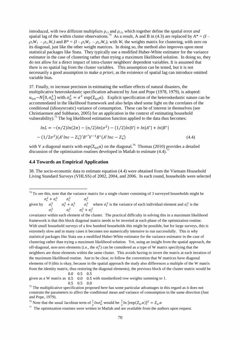
70

introduced, with two different multipliers ρc1 and ρc2, which together define the spatial error and

spatial lag of the within cluster observations.74

As a result, A and B in (4.3) are replaced by A* = (I –

1W1 – c1Wc) and B* = (I – 2W2 – c2Wc), with Wc the weights matrix for clustering, with zero on

its diagonal, just like the other weight matrices. In doing so, the method also improves upon most

statistical packages like Stata. They typically use a modified Huber-White estimator for the variance

estimator in the case of clustering rather than trying a maximum likelihood solution. In doing so, they

do not allow for a direct impact of intra-cluster neighbors' dependent variables. It is assumed that

there is no spatial lag from the cluster variables. This assumption can be tested, but it is not

necessarily a good assumption to make a priori, as the existence of spatial lag can introduce omitted

variable bias.

37. Finally, to increase precision in estimating the welfare effects of natural disasters, the

multiplicative heteroskedastic specification advanced by Just and Pope (1978, 1979), is adopted:

Explicit specification of the heteroskedastic nature can be

accommodated in the likelihood framework and also helps shed some light on the correlates of the

conditional (idiosyncratic) variance of consumption. These can be of interest in themselves (see

Christiaensen and Subbarao, 2005) for an application in the context of estimating household

vulnerability).75

The log likelihood estimation function applied to the data thus becomes:

(4.4)

with V a diagonal matrix with on the diagonal.76

Thomas (2010) provides a detailed

discussion of the optimization routines developed in Matlab to estimate (4.4).77

4.4 Towards an Empirical Application

38. The socio-economic data to estimate equation (4.4) were obtained from the Vietnam Household

Living Standard Surveys (VHLSS) of 2002, 2004, and 2006. In each round, households were selected

74

To see this, note that the variance matrix for a single cluster consisting of 3 surveyed households might be

given by

where is the variance of each individual element and

is the

covariance within each element of the cluster. The practical difficulty in solving this in a maximum likelihood

framework is that this block diagonal matrix needs to be inverted at each phase of the optimization routine.

With small household surveys of a few hundred households this might be possible, but for large surveys, this is

extremely slow and in many cases it becomes too numerically intensive to run successfully. This is why

statistical packages like Stata use a modified Huber-White estimator for the variance estimator in the case of

clustering rather than trying a maximum likelihood solution. Yet, using an insight from the spatial approach, the

off-diagonal, non-zero elements (i.e., the ) can be considered as a type of W matrix specifying that the

neighbors are those elements within the same cluster. This avoids having to invert the matrix at each iteration of

the maximum likelihood routine. Just to be clear, to follow the convention that W matrices have diagonal

elements of 0 (this is okay, because in the spatial approach the study also differences a multiple of the W matrix

from the identity matrix, thus restoring the diagonal elements), the previous block of the cluster matrix would be

given as a W matrix as

with standardized row weights summing to 1.

75 The multiplicative specification proposed here has some particular advantages in this regard as it does not

constrain the parameters to affect the conditional mean and variance of consumption in the same direction (Just

and Pope, 1979). 76

Note that the usual Jacobian term of

77 The optimization routines were written in Matlab and are available from the authors upon request.

71

using a 3-stage sampling process.78

These three survey waves provide high quality and nationally

representative household information on household consumption and income, their demographic

characteristics, health status, educational achievements, asset holdings and the availability of public

services in the community. The latter is obtained from the community survey which was fielded in

parallel to the household surveys. The questions in the VHLSS were similar throughout the different

surveys rendering them highly comparable. The surveys were conducted each year between May and

November of the survey year, with expenditures referring to the past 12 months.

39. Real total per capita expenditure less per capita expenses on health care is taken as dependent

variable. Health expenditures are subtracted as the study also controls for the effect of idiosyncratic

health shocks, proxied by the number of days spent ill in bed over the past year by senior adults,

adults and children respectively. Inclusion of health expenditures in the overall expenditure measure,

which are highly correlated with illness and not routine or maintenance health outlays, might

perversely suggest an increase in welfare following sickness. The expenditure data are expressed in

January 2002 prices using the CPI provided by the Government Statistical Office. They are also

corrected each year for regional and rural/urban differences across the eight regions.

40. A series of standard household demographics (household size, the dependency ratio, the age,

gender, educational status of the household head79

) are included to control for household

characteristics in determining a household‘s consumption level. In this context, controlling for

ethnicity is especially important as poverty is increasingly concentrated among ethnic minorities,

often located in Vietnam‘s mountainous areas. While productive assets affect the capacity of a

household to generate income and thus its consumption level, current asset levels may be

simultaneously determined with consumption, as the disposal of assets (e.g. livestock) may be relied

upon to cope with disasters, or they may reflect destruction by the disasters, leading to an

underestimate of the welfare effects of the latter. In the absence of information of asset ownership

prior to the survey, only those assets that display limited variation over time were included such as the

amount of land owned and an indicator variable indicating whether the household owns a house or

not.

41. To reflect access to public services, indicator variables are included that take the value of one if

clean water80

, sanitary latrines,81

or electricity are present in the community, and zero otherwise. To

proxy a household‘s integration in the overall economy, the community data were further augmented

with the distance of the centroid of the community (in meters) to the nearest part of the nearest

primary or secondary road, as designated in the VMAP0 dataset (NIMA, 1997). These measures were

computed that using Arc View 3.2. In addition, the estimated travel time to the nearest town or city of

at least 25,000 people, the nearest city of at least 100,000 people, and the nearest city of at least

500,000 people were included. The travel times were computed in Arc View from a friction grid that

78

Communes (the primary sampling units) were selected in the first stage with a probability proportionate to

population size based on the 1999 Population census. On average, a commune contains 1,600 households.

Subsequently, three enumeration areas (EAs), containing about 100 households each, were randomly selected

within each commune. One of these EAs would be used to draw a sample of households in each VHLSS during

the final (third) stage. In, 2002, this resulted in a sample of 29,530 households across 2,910 communes (EAs)

(25 households per EA in 75% of the EAs and 5 in the remaining 25%). In 2004 and 2006, three households

were selected per EA, resulting in 9,189 households each year in 3,061 communes. Phung and Nguyen (2008)

provide a detailed description of the questionnaire and survey design. 79

0 refers to no degree, 1 to primary school, 2 to lower secondary school, 3 to higher secondary school, 4 to

short-term technical worker, 5 to long-term technical worker, 6 to professional secondary school, and 7 to

college diploma and above. 80

Two sources of water are typically distinguished in Vietnam: water for direct human consumption (drinking,

cooking), and water for sanitation and maintenance purposes (washing clothes and bathing). Water is

considered clean if it comes from (1) private tap water inside the house, (2) private tap water outside the house,

(3) public tab water, (4) water pumped from deep drill wells, (5) water from hand-dug and reinforced wells, (6)

rain water, (7) purchased water, or (8) water from a water tank. 81

Sanitary latrines include flush toilets with septic tank/sewage pipes, suilabh toilets, and double vault compost.

72

assigned differing travel times to various classes of roads, urban areas, water bodies, off-road, and

crossing international boundaries.82

42. To further control for geological and agro-ecological characteristics at the community level,

elevation figures were included, taken from the GLOBE 1 kilometer elevation database (GLOBE

Task Team et al. 1999). Elevation differences were also incorporated as a measure of terrain

roughness. These were computed using the SRTM3 data (Jarvis et al., 2006) by subtracting the

minimum elevation in a 1 kilometer grid from the maximum elevation in the 1 kilometer grid. Finally,

urban/rural and regional indicator variables help capture unobserved (time invariant) location specific

characteristics related to the urban and rural livelihood systems as well as those related to regional

variation in the agro-ecological, economic and political environment. Year dummies were included to

control for the survey year.

43. The disaster data were mapped into the household survey data at the commune level, which are on

average only 30,3 kilometer squared.83

More precisely, the centroid for each commune was identified

and given the highly covariate character of the different disasters, the state of nature observed at that

point in the disaster maps was assumed to be the state of nature experienced by all the VHLSS

households in that commune. It emerges that while most households have some limited drought risk,

twenty percent of the population has at least 30 percent chance of being flooded each year (Figure

4.11). At the same time, about two fifths of the population will never be affected by a flood and

storms pass by about half the population.

44. Given the concentration of flood events, it does not come as a surprise that there is a strong

intertemporal correlation in the occurrence of floods (0.44 for flash floods and 0.55 for riverine

floods), i.e. households experiencing a flood his year also have a high chance of experiencing one the

following year (Table C2). As expected, there is also a correlation between the statistical frequency

with which extreme weather events happen (their incidence) and their actual occurrence during the

current or previous survey years, a correlation which is most pronounced for floods. Finally, some

bunching of events is also observed, with households subjected to a hurricane, often also hit by flash

floods, as indicated by the correlation coefficient of 0.55 between the incidence of flash floods and the

incidence of hurricanes. Hurricanes thus manifest themselves partly through localized flooding.

Riverine floods on the other hand appear negatively correlated with flash floods and hurricanes.

Finally, note that a higher incidence of drought does not exclude the occurrence of floods within the

same year as indicated by the positive correlation between the incidence of droughts and floods (and

hurricanes).

45. The bunching of the disasters underscores the importance of considering their effect separately,

but jointly in the regression analysis. Potential persistence in the effect is examined through

consideration of both the current and one year lagged events. Finally, to separate out the potential

effects of adaptation from the immediate welfare effects from current events, the regressions also

control for the frequency with which the different events occurred.

82

The VMAP0 (NIMA, 1997) was used to obtain data on three classes of roads: 1) divided highways; 2)

primary/secondary roads; 3) paths or trails. For rivers and lakes, the CIA World Data Bank II (CIA, 1972) was

used. The population centers are from the GRUMP settlement points dataset (CIESIN et al., 2004a) and the

World Gazetteer database (Helders, 2005). Urban boundaries are from the GRUMP urban extents database

(CIESIN et al., 2004b). The international boundaries are from the World Bank mapping office. 83

To maintain confidentiality, the geographic coordinates of each household in the VHLSS are not made

publicly available, only the shapefiles for the different communes surveyed.

73

4.5 Welfare Effects of Natural Disasters in Vietnam

46. To benchmark the results, Table 4.1 (column 1) presents the estimated OLS coefficients84

of a

standard consumption model augmented with information on the present and lagged occurrence of the

different extreme weather events (droughts, localized and riverine floods, hurricane force winds).

These are subsequently augmented with data on the frequency of their occurrence (column 2) and

interaction terms between the extreme events and the distance to cities with more than 500,000

inhabitants to capture geographical diversity in the effects (column 3). The Maximum Likelihood

estimates which also correct for spatial correlation (in addition to heteroskedasticity and cluster

design) are in column 4. The following cut-offs were settled on to identify an event as extreme:

rainfall 20 percent below the long run median for drought; at least one episode of more than 300 mm

rainfall in 5 consecutive days for excess rain/localized flooding; DFO recorded floods within 2 m

elevation difference from the major rivers or coast line; and areas affected by 65 knot (or 118

km/hour) hurricane wind force.

47. The regressions display high explanatory power (R-squared between 55 and 60 percent) and the

estimated coefficients on the different household and community characteristics are consistent with

those reported in the literature. This provides confidence in the base results.85

Larger households

with more dependents and belonging to ethnic minorities are poorer, while the more experienced and

more educated households with more land and in possession of a house enjoy higher living standards.

Illness of adult household members (not for children or elderly) tends to be negatively associated with

consumption levels, though it is only statistically significant for the spatially corrected ML estimates.

Households in communities with better sanitary conditions (sanitary living water and sanitary latrines)

and better road access are also richer, while households located on steeply sloped areas tend to be

poorer. Households in urban areas are on average about 30 percent richer, with levels of consumption

declining the further away from the urban center and the gradients steepening the larger the urban

center. Consistent with the steep GDP growth observed in Vietnam during the survey period,

household consumption levels (in real terms) increase substantially between the survey years, as

reflected in the large and statistically significant coefficients on the year dummy variables.

The more exposed to natural disasters, the poorer households tend to be

48. Turning to the welfare effects of weather events, household welfare is substantially affected by

natural disasters, but at first sight, not always in the direction expected. When included without

controls for exposure (Table 4.1, column 1), current droughts, localized and riverine floods appear

positively correlated with household welfare, with the occurrence of a localized flood last year also

increasing welfare, with the lagged effects of riverine floods exercising a dampening effect on

household welfare. However, when the frequency of extreme events in each locality is included

together with their interaction with the current and lagged occurrence of the event (column 2), a

different picture emerges.

49. Welfare is lower in areas frequently exposed to droughts and hurricanes, while (surprisingly) it

appears to increase welfare in areas frequently exposed to excess rain, with no discernable effect in

frequently inundated riverine areas. Second, the direction of the immediate welfare effects of current

and lagged events also changes when interacted with the frequency of their occurrence. Current

droughts, localized and riverine floods no longer increase welfare and excess rainfall in the current

year is now negatively related with consumption, at least when excess rain is not a regular

phenomenon. The signs and statistical significance of past weather events, reflecting the lagged

welfare effects, also change when they are interacted with their frequency.

84

These were obtained from the pooled 2002, 2004, and 2006 VHLSS data with standard corrections for

heteroskedasticity and clustered survey design using the Hubert-White estimator provided in STATA. 85

The comprehensive controls for community (and household) characteristics help protect the natural disaster

variables from omitted variable bias. As the survey comprises more than 3000 communities, each surveyed at

least two times, overfitting is not considered a concern. Note also that the number of controls is in effect still

substantially less than when estimating a household or community fixed effect regression.

74

50. Frequent exposure may induce the adoption of low risk, low return portfolios (Eswaran and

Kotwal, 1990; Rosenzweig and Binswanger, 1993), but the associated welfare loss could also reflect

accumulated asset loss (Carter and Barrett, 2006), issues further discussed below. Poor people may

also concentrate in areas considered too risky to live in. Given the myriad of household and

environmental controls that already capture household wealth, such as education, ownership of land

and housing, access to public infrastructure and amenities, proximity to urban centers as well as agro-

ecological conditions (elevation and slope), the latter interpretation of the results is less likely. The

results in columns (1) and (2) underscore especially the importance of controlling for the frequency of

exposure in studying the immediate and lagged welfare effects of natural disasters.

Those further away from large urban centers are poorer, but also tend to suffer less from being

regularly confronted with natural disasters

51. The welfare effects likely also differ depending on the proximity to large urban centers (Table 4.1,

column 3). In particular, interaction of the different events with the distance (in tenths of hours) to

cities with more than 500,000 inhabitants suggests that the welfare effects gradually change away

from these large urban centers. Locations further away are typically less affected. For example,

while areas frequently hit by drought are less wealthy, frequent exposure to droughts appears less

damaging in terms of welfare loss further away from the large cities, that is, after controlling for the

welfare reducing effect of living far away from urban centers. Similarly, areas located in storm prone

areas further away from the urban centers are less affected than those in storm prone areas close to the

city. A similar phenomenon is observed when it comes to localized flooding –with frequent exposure

less damaging among those further out.

52. Economies and livelihoods become more rural and agriculturally oriented further away from the

metropolitan areas. Asset holdings and the share of agricultural land irrigated typically declines

(Table C3) and the support systems weaken. In particular, households further away tend to be less

likely to receive remittances from abroad and the amounts received tend to be smaller. And while

they are as likely to receive domestic remittances and even more likely to receive disaster relief, the

latter is still rare (only 12 % of the households received disaster relief during the 2002-2004-2006

surveys) and it usually comes in much smaller amounts than the relief received by those close to the

metropolitan centers. Taken together these descriptive suggests that households further away are not

only more exposed ex ante (at least to drought) but also have lower capacity to cope with natural

disaster ex post (less assets/savings and less effective support systems). This may have induced them

to adopt portfolios that are more resilient to damage from natural disasters, though portfolios that are

also less remunerative , as indicated by the steep declining gradient in household welfare as one

moves away from the metropolitan centers.

53. From this perspective, the reverse finding on riverine flooding comes as a surprise. Out of the 4

disasters considered, only frequent exposure to riverine flooding is associated with an increase (as

opposed to a decline) in living standards, with its benefits declining as one moves away from the

major metropolitan centers. In this case, regular flooding seems to have induced a superior livelihood

system, at least among those closer to the metropolitan area. This is mostly in regard to households in

the Mekong River Delta, that have their livelihood systems built around floods (―living with flood‖,

very much as in Bangladesh, Beck, 2005). Comparison of self-reported flood measures with the

riverine flood measure used here (taken from the DFO) supports this interpretation. The flood

incidence based on the latter measure is much larger than the flood incidence based on the former,

indicating that not all floods recorded in DFO are actually also experienced as negative events by the

households themselves. It is not so much the flooding as such which is detrimental, but rather its

duration and level, rendering only a subset of the DFO observed floods really damaging.

Immediate, lagged and persistent welfare effects by event

54. For a more detailed shock by shock comparison of the welfare effects, the study turns to the

Maximum Likelihood welfare estimates, which also correct for spatial correlation (Table 4.1, column

4). While they qualitatively correspond to the OLS estimates in column 3, the size of the effects

75

changes at times substantially and the coefficients are also more precisely estimated, yielding

additional insights. This is expected given that both the tests for spatial lags and errors (not reported

here) point to the existence of spatial correlation (within and beyond the cluster). To provide some

further intuition to the findings, it is simultaneously explored how households cope with each of the

shocks. In particular, the immediate, lagged and persistent effects of the different natural disasters on

a household‘s asset holdings, its reception of official disaster relief and domestic and foreign

remittances, and its degree of income diversification as captured in the Herfindahl index,86

are given

in Table 4.2. The effects of natural disasters on asset holdings and income diversification are

estimated using OLS with suitable corrections for heteroskedasticity and cluster design, while left

censored tobits are used for the household assistance regressions, as many households did not receive

any assistance/remittances. To control for household, community and environmental characteristics,

the same controls are used as in the household welfare regressions above. The ML results are

repeated in the first column (Table 4.2, column 1) to facilitate the discussion.

Droughts reduce welfare, though mainly among those with few irrigated plots

55. As before, there are no statistically significant signs of immediate or lagged effects of droughts.

Further investigation using the 2004 and 2006 survey years for which information on irrigation is also

available, shows that irrigation provides effective protection against droughts. In particular,

households with no irrigated plots see their per capita consumption decline by 16 percent on average

the year of the drought, while those with all their plots irrigated (the majority of the sample)

experiencing only a 3 percent loss in welfare. In other words, irrigation proves quite effective in

protecting households from drought. No lagged effect of droughts is observed. Self insurance

through asset disposal (which shows up with a lag,Table 4.2, column 2) and income diversification

(lower Herfindahl index), especially in drought prone areas, enables households to further soften the

blow of immediate drought shocks. Yet, this also erodes their asset base over time, consistent with

the lower welfare observed in drought prone areas. The loss can be substantial — households in areas

with a 10 percentage point higher frequency of drought are on average 12 percent poorer — though

the majority of households only experience a drought once a decade, with only two percent facing a

drought every three to five years.

56. Interestingly, the welfare loss associated with frequent drought occurrences declines as one moves

away from the metropolitan areas. This is likely related to the somewhat larger responsiveness of

official relief efforts to current drought events in those more remote areas (albeit with lower amounts

disbursed on average),87

which appears to mitigate the need for self insurance through asset disposal,

as suggested by the lower asset loss experienced in less urbanized areas (positive coefficient on the

interaction term of lagged drought and distance to large city—column 2). Over time this yields lower

accumulated asset loss in the more remote areas (column 2) and less severe welfare loss (column 1)

than in the areas closer to the metropolitan areas. The disaster relief systems appears to enable these

households to remain more specialized (higher Herfindahl index), i.e. more agriculture focused, than

those in other drought prone areas closer to the metropoles, suggesting that the relief efforts also help

in mitigating the effects of droughts, even though the amounts disbursed tend to be smaller than

among those closer to the metropoles.

Localized floods cause an immediate welfare loss, which households largely recuperate thereafter

57. Heavy rainfall has an immediate welfare reducing effect, by 7.7 percent on average (Table 4.2,

column 1), likely through the destruction of assets (Table 4.2, column 2), though less in areas, which

are frequently exposed, and thus better adapted, or those further away from the metropoles. There is

86

The Herfindahl index is a measure of income diversification, defined as the sum of the squares of the different

income shares. It ranges between one and zero, with 1 indicating full specialization and lower values pointing

to increasingly diversified income portfolios. 87

Indicated by the jointly positive and statistically significant coefficients on current drought events and their

interaction term with distance away from the metropolitan areas when 2 hours or more away from the

metropolitan area.

76

also a lagged welfare increasing effect of heavy rainfall. Heavy rainfall often goes hand in hand with

landslides which can cause substantial damage to infrastructure, property and capital. When not too

severe or not too frequent, households can take advantage of such asset loss to accelerate replacement

of their assets by better, more productive ones, accelerating their return to their normal growth path,

as postulated in the vintage capital growth models (Hallegate and Dumas, 2009). Households in

areas more frequently affected by localized floods tend to experience lower levels of consumption,

though again, less severe so among those in flood prone areas further away.

58. Overall the welfare losses from frequent exposure to excess rain are only one fourth to one fifth

(-0.28/-1.26) those brought about by regular exposure to rainfall shortages. Lower net asset loss (the

immediate negative effects largely compensated by technically better replacements in the next period

helps understand the difference in the welfare effects of rainfall shortages and rainfall excesses (Table

4.2). While the destruction of assets associated with excess rain does not lead to higher welfare levels

altogether, their replacement with better more productive alternatives, especially in areas that are not

frequently confronted with excess rain (see the negative coefficient on interaction term of lagged

localized flood and excess rain frequency in column 2) can mitigate their negative effects. Droughts

on the other hand, do not induce an immediate asset loss as such (beyond livestock loss). Assets are

disposed off to cope with the shocks, smoothing consumption in the current period, but eroding the

household‘s coping capacity over time, consistent with the larger negative effect of the frequent

occurrence of droughts on asset holdings (coefficient equals -3.4, the largest among all disasters

considered), and by extension on consumption. Larger official relief efforts in frequently flooded

areas closer to the larger cities may further attenuate the welfare loss compared with those related to

water shortages. Households do not appear to change their income portfolios in response to heavy

rainfall—none of the coefficients on the localized flood variables and their interaction terms are

statistically significant, with the exception of one, whose coefficient is very small.

While households learned to live with riverine floods, severe floods can cause substantial damage

59. The occurrence of a riverine flood reduces household welfare on average with a combined 23

percent, by 5.8 percent immediately and by 17.2 percent in the subsequent year, indicating that it

takes some time for the full effect to be felt. But as indicated above, not all riverine floods recorded

in DFO make for a negative experience, and households in areas prone to riverine floods appear on

average even slightly better off. They experience less immediate welfare loss (positive coefficient on

interaction term between flood frequency and current flood event—column 1, Table 4.2) and dispose

less of their assets to cope with the effects (positive coefficient on interaction term with lagged

riverine flood – column 2, Table 4.2), likely linked to the much better provision of disaster relief in

regularly flooded areas. While the disaster relief in the flood prone areas prevents the erosion of the

asset base (no loss of assets in frequently affected areas—column 2), it is nonetheless not sufficient to

prevent a substantial 17 percent temporary reduction in their consumption welfare loss based on the

floods recorded in this sample. This loss manifests itself with a lag, together with lagged reduction in

the asset base.

60. Households in flood prone areas away from the urban centers on the other hand appear more

negatively affected by riverine floods. They receive much less disaster assistance, find themselves

over time with a lower asset base (negative coefficient on interaction distance to city and flood

frequency), resulting in a long term welfare loss (negative coefficient interaction term distance to city

and flood frequency—column 1). Households also cope with the lagged effects of shocks through

income diversification, especially closer to the cities.

Hurricane force winds inflict immediate and lasting damage to household welfare.

61. The occurrence of a hurricane is associated with a 52 percent immediate welfare loss inside cities

with more than 500,000 inhabitants, a potential 16 percent loss in the subsequent year, and a 20

percent reduction in welfare in areas with a 10 percentage point higher chance of being hit by

hurricane wind forces. Furthermore, unlike with (localized and riverine) floods the immediate effects

are not mitigated in areas that are more frequently hit, i.e. there is no adaptation. Rather the opposite,

77

the immediate and lagged effects are, if anything, even more detrimental, indicating that households

have not been able to adapt to and that the official disaster relief system has not been effective in

dealing with hurricane forces winds in Vietnam. Second, the damage is less severe the further away

from the urban centers. This can be expected given the larger concentration and reliance of the

economy and livelihoods on infrastructure in the more urban economies. Official and private

transfers have largely been unresponsive to storm related disasters (columns 3-5, Table 4.2).

Similarly portfolio choice remains largely unaffected in the face of storms, with the exception of some

lagged portfolio diversification in areas frequently affected.

62. Summarizing the key insights regarding the allocation of disaster relief, one of the key ex post

policy responses to disasters, households further away from the larger urban centers (more than

500,000 inhabitants) are on average more likely to receive disaster aid (see positive coefficient on log

hours to 500k city). While the amounts received tend to be smaller, it does help in coping with the

welfare loss. Furthermore, relief efforts appear not to be sustained much beyond the first year. The

disaster relief systems appear especially well developed in frequently flooded areas (both localized

and riverine or coastal) close to the major urban centers. Official disaster assistance is not given

following hurricane force winds. There are no clear systematic patterns with respect to the reception

of domestic or foreign remittances. Sectoral income diversification does not emerge as a major

coping strategy, with the exception of the larger income diversification observed in drought prone

areas closer to the urban centers. Asset losses, which can result from direct damage or through asset

disposal to self insure, often show up with a delay and tend to be less severe further away from the

urban centers.

63. In conclusion, while households largely manage to cope with drought events, often through asset

disposal, but especially through irrigation, the frequent occurrence of droughts erodes their capacity to

cope with them over time. These result in substantial welfare loss among households in drought prone

areas closer to the urban centers. Households in drought prone areas further away from the urban

capitals also suffer, but less as they manage to hang on to their assets better because of drought

responsive relief efforts. Localized flooding exerts an immediate 7 percent toll on welfare though

much of that loss appears to be recuperated the next year potentially through replacement of the lost

asset base by better more productive ones, at least among those that are not frequently hit. The latter

tend to suffer less immediately, partly through the reception of disaster aid, but they also benefit less

from the faster adoption of more productive assets, likely resulting in some asset erosion over time

and lower consumption levels (though to a lesser extent than in the case of regular rainfall failure).

The damage from frequent exposure to localized floods is again less severe among those further away

from the urban centers, as they experience less asset loss, while receiving more immediate disaster

relief. Riverine floods can cause substantial welfare damage (23 percent), especially among those not

frequently exposed, who tend to be better served by disaster relief, at least when living close to the

urban centers. Finally, the largest damage is inflicted by hurricane force winds, with both regular

exposure and proximity to the urban centers exacerbating the welfare losses substantially.

4.6 Concluding Remarks

64. Understanding how natural disasters affect human welfare is an increasingly pressing concern, not

least in Vietnam, which ranks among the most disaster prone countries in the world. This study

illustrates a methodology to study the welfare effects of such events in a country specific setting using

spatially disaggregated disaster maps derived from primary meteorological data combined with

nationally representative geo-referenced household survey data. By deriving the spatially

disaggregated event and hazard maps directly from the meteorological data, issues of endogeneity in

estimating the effect of such events on consumption are mitigated. The event and hazard maps

provide also useful tools for policy and project planning. In addition, in estimating the welfare effects,

spatial correlation was accounted for. While the latter is routinely ignored, this is less suitable in

empirical examinations of the household welfare effects of spatially disaggregated disasters whose

effects regularly permeate the economy through product (food prices) and factor (labor) markets.

78

65. The econometric results suggest that households in Vietnam largely manage to cope with the

immediate effects of drought events, through irrigation. However, the frequent occurrence of droughts

erodes their capacity to cope with them, resulting in substantial welfare loss especially among

households in drought prone areas closer to the urban centers, where disaster relief is less pronounced.

Localized floods exert important welfare losses, on average an estimated at 7 percent, though much of

that loss appears to be recuperated through capital replacement in the subsequent year, at least among

those who are only occasionally affected by such floods. Those who are frequently affected suffer

more, though the long run effects from frequent exposure to localized floods are substantially less

than those from frequent exposure to droughts, partly due to a responsive relief system in the more

urban areas that are frequently affected. Riverine floods cause substantial welfare damage (23

percent) in the short run, though less so among households who are frequently exposed. Not only do

they tend to be much better served by disaster relief, especially when close to the metropolitan

centers, it is important to note that not all riverine floods recorded in DFO are experienced as negative

events, as households built their livelihood systems around them, especially close to the metropolitan

areas. They learned to live with floods. Finally, the largest damage is inflicted by hurricane force

winds, with regular exposure and proximity to the urban centers, both of which exacerbate the welfare

losses substantially.

66. Overall, the study shows that there is promise in using meteorological data to construct spatially

disaggregated weather event and weather hazard maps, the first objective of the study. Such data are

becoming increasingly available and natural event and hazard maps have also important direct

applications for policymakers beyond their use in estimating the welfare effects of disasters. The fine-

tuning and validation of such maps is an important area for further research. Second, there are

important long run negative effects of being regularly confronted with natural disasters. Third, short

run losses can be substantial, with hurricanes causing most havoc. Fourth, there are signs of

adaptation, with frequent exposure to localized and riverine floods reducing the welfare losses

associated with these events, partly through the development of effective disaster relief systems.

There is however no adaptation to hurricanes, rather the contrary, with high frequency of hurricanes

exacerbating the losses from particular events. Fifth, those further away from the large urban centers

often enjoy more immediate disaster relief which appears to mitigate the current effects of natural

hazards, underscoring the importance of effective disaster relief systems. In the absence of further

support systems, they likely also adopted less risky, but also less remunerative portfolios. Sixth, the

disaster relief systems have largely eluded areas affected by hurricane force winds so far, an important

area of attention for Vietnamese policymakers.

79

Figure 4.1 Regions of Vietnam

80

Figure 4. 2 Rainfall maps using inverse distance weighing and inverse elevation difference weighting display close resemblance

Figure 4.2a: Rainfall prediction using inverse

distance squared from 5 nearest station data

only, June 2006

Source: Thomas et al. (2010)

Figure 4.2b: Rainfall prediction using elevation

difference weighting for 10 nearest stations

only, June 2006

Figure 4.2c: Rainfall prediction from

regression analysis, June 2006

81

Figure 4. 3 Deviations from median annual rainfall for each year 2001 to 2006.

2001 2002 2003

2004 2005 2006

Source: Thomas et al. (2010).

82

Figure 4.4 Proportion of years with 20 percent shortfall in median annual rainfall

Source: Thomas et al. (2010).

83

Figure 4.5 Localized flooding for each year 2001 to 2006.

2001 2002 2003

2004 2005 2006

Source: Thomas et al. (2010)

84

Figure 4.6 Proportion of years in which 300 mm of rain fell in a consecutive 5-day period

Source: Thomas et al. (2010)

85

Figure 4.7 Riverine and coastal flooding for each year 2001 to 2006.

2001 2002 2003

2004 2005 2006

Source: Dartmouth Flood Observatory (2008) and author's calculations using Hydrosheds and GLOBE.

86

Figure 4.8 Proportion of riverine and coastal flooding 1985-2007.

87

Figure 4.9 Hurricane force winds associated with tropical cyclones for 2001 to 2006.

2001 2002 2003

2004 2005 2006

Source: UNEP / GRID (2007) and author's calculations.

88

Figure 4.10 Proportion of years with hurricane force winds

Source: Thomas et al. (2010), based on GNV199 (UNEP/GRID-Europe, 2007a).

89

Figure 4.11 Most people are exposed to droughts, but infrequently; floods affect a sizeable

population often, and a large population never; hurricanes pass by most and infrequently affect

others.

0

0.1

0.2

0.3

0.4

0.5

0.6

0.7

0.8

0.9

1

0 20 40 60 80 100

like

liho

od

of

eve

nt

Population (cumulative %)

drought

flashflood

riverine flood

tropical storm

90

Table 4. 1 Extreme weather events can have substantial negative effects on household welfare,

immediately and through adaptation over time, with adaptation and disaster relief often mitigating

the immediate losses

Dependent variable:

log expenditure/capita

(excl. health expenditure)

OLS with Hubert-White

heteroskedasticity and cluster design

correction

ML corrected for

spatial correlation,

cluster design and

heteroskedasticity

(1) (2) (3) (4)

parameter/

t-value

parameter/

t-value

parameter/

t-value

parameter/

t-value

Extreme weather event in community

Droughts

Drought this year 0.0309*** 0.0016 -0.0671 0.0245

2.92 0.06 -1.04 0.58

Drought this year*drought frequency 0.3023 0.2918 0.0704

1.48 1.39 0.46

Drought this year*ln(hours) from 500k

city

0.0177 -0.0006

1.23 -0.06

Drought last year 0.0118 0.004 0.1159 -0.0008

0.44 0.06 0.45 -0.01

Drought last year*drought frequency 0.1253 0.0179 -0.1257

0.35 0.05 -0.45

Drought last year*ln(hours) from 500k

city

-0.0212 0.0111

-0.39 0.31

Drought frequency (proportion) -0.5241*** -2.5466*** -1.2609***

-4.74 -5.54 -4.25

Drought frequency*ln(hours) from 500k

city

0.5486*** 0.2845***

4.54 3.72

Excess rain

Excess rain this year 0.0529*** -0.0658*** -0.1552*** -0.0768**

4.14 -2.76 -2.92 -2.21

Excess rain this year*Excess rain

frequency

0.1998*** 0.0798 0.0685*

4.24 1.28 1.90

Excess rain this year*ln(hours) from 500k

city

0.0377** 0.0159

2.2 1.49

Excess rain last year 0.0521*** 0.0836*** 0.1657** 0.1337***

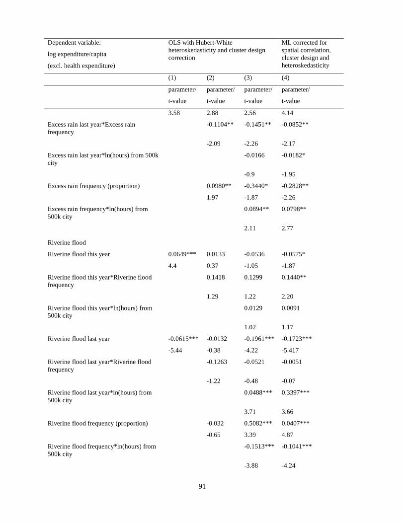
91

Dependent variable:

log expenditure/capita

(excl. health expenditure)

OLS with Hubert-White

heteroskedasticity and cluster design

correction

ML corrected for

spatial correlation,

cluster design and

heteroskedasticity

(1) (2) (3) (4)

parameter/

t-value

parameter/

t-value

parameter/

t-value

parameter/

t-value

3.58 2.88 2.56 4.14

Excess rain last year*Excess rain

frequency

-0.1104** -0.1451** -0.0852**

-2.09 -2.26 -2.17

Excess rain last year*ln(hours) from 500k

city

-0.0166 -0.0182*

-0.9 -1.95

Excess rain frequency (proportion) 0.0980** -0.3440* -0.2828**

1.97 -1.87 -2.26

Excess rain frequency*ln(hours) from

500k city

0.0894** 0.0798**

2.11 2.77

Riverine flood

Riverine flood this year 0.0649*** 0.0133 -0.0536 -0.0575*

4.4 0.37 -1.05 -1.87

Riverine flood this year*Riverine flood

frequency

0.1418 0.1299 0.1440**

1.29 1.22 2.20

Riverine flood this year*ln(hours) from

500k city

0.0129 0.0091

1.02 1.17

Riverine flood last year -0.0615*** -0.0132 -0.1961*** -0.1723***

-5.44 -0.38 -4.22 -5.417

Riverine flood last year*Riverine flood

frequency

-0.1263 -0.0521 -0.0051

-1.22 -0.48 -0.07

Riverine flood last year*ln(hours) from

500k city

0.0488*** 0.3397***

3.71 3.66

Riverine flood frequency (proportion) -0.032 0.5082*** 0.0407***

-0.65 3.39 4.87

Riverine flood frequency*ln(hours) from

500k city

-0.1513*** -0.1041***

-3.88 -4.24

92

Dependent variable:

log expenditure/capita

(excl. health expenditure)

OLS with Hubert-White

heteroskedasticity and cluster design

correction

ML corrected for

spatial correlation,

cluster design and

heteroskedasticity

(1) (2) (3) (4)

parameter/

t-value

parameter/

t-value

parameter/

t-value

parameter/

t-value

Hurricane force wind

Hurricane force wind this year 0.0185 -0.0726 -0.4159 -0.7309***

0.79 -1.16 -1.14 -2.93

Hurricane force wind this year*Hurricane

force wind frequency

1.3281** 0.0739 -0.9634

2.08 0.09 -1.41

Hurricane force wind this year*ln(hours)

from 500k city

0.0886 0.1737***

1.07 2.99

Hurricane force wind last year 0.0384 0.1967* 0.0658 -0.1642

1.29 1.95 0.29 -0.96

Hurricane force wind last year*Hurricane

force wind frequency

-1.1792 -1.197 -1.4028**

-1.23 -1.28 -2.06

Hurricane force wind last year*ln(hours)

from 500k city

0.0281 0.0762**

0.54 1.97

Hurricane force wind frequency

(proportion)

-0.5151*** -2.0504*** -2.1608***

-3.42 -4.83 -7.45

Hurricane force wind frequency*ln(hours)

from 500k city

0.4566*** 0.4584***

3.68 5.79

Household characteristics

log of household size -0.2419*** -0.2447*** -0.2474*** -0.2832***

-36.06 -36.83 -37.38 -56.634

dependency ratio -0.0046*** -0.0046*** -0.0046*** -0.0047***

-28.82 -28.96 -28.92 -36.03

1 if ethnic minority; 0 otherwise -0.2388*** -0.2411*** -0.2396*** -0.2422***

-16.32 -16.49 -16.66 -29.05

1 if household head is female 0.0123* 0.0104* 0.0081 0.0005

1.93 1.65 1.3 0.10

log of age of household head 0.1233*** 0.1236*** 0.1217*** 0.1317***

13.44 13.54 13.47 18.71

93

Dependent variable:

log expenditure/capita

(excl. health expenditure)

OLS with Hubert-White

heteroskedasticity and cluster design

correction

ML corrected for

spatial correlation,

cluster design and

heteroskedasticity

(1) (2) (3) (4)

parameter/

t-value

parameter/

t-value

parameter/

t-value

parameter/

t-value

education household head = 1 if

primary school 0.1556*** 0.1564*** 0.1553*** 0.14073***

22.64 22.91 22.96 26.99

Lower secondary school 0.2618*** 0.2659*** 0.2659*** 0.2524***

33.02 33.83 34.16 44.32

Higher secondary school 0.4159*** 0.4187*** 0.4186*** 0.39063***

37.96 38.45 39 47.55

Short-term technical worker 0.4881*** 0.4993*** 0.5066*** 0.47005***

32.19 33.25 33.84 37.51

Long-term technical worker 0.5566*** 0.5626*** 0.5668*** 0.5312***

38.19 38.83 39.74 44.43

Professional secondary school 0.5787*** 0.5832*** 0.5833*** 0.55974***

37.36 37.69 37.8 42.96

College diploma and above 0.8133*** 0.8130*** 0.8099*** 0.76219***

51.35 52.7 54.59 65.25

Days ill in bed, senior household members 0.0001 0.0001 0.0001 0.0000

0.71 0.67 0.6 0.47

Days ill in bed, adult household members -0.0002 -0.0002 -0.0002 -0.0002***

-1.42 -1.45 -1.57 -2.07

Days ill in bed, children 0.0001 0.0002 0.0002 0.0002

0.74 0.84 0.84 0.94

Own a house (1=yes; 0=no) 0.1393*** 0.1415*** 0.1493*** 0.1592***

9.01 9.28 10.31 15.40

Own land (1=yes;0=no) -0.7036*** -0.6848*** -0.6848*** -0.7334***

-21.83 -21.67 -21.77 -37.63

Areas of land owned (squared metres) 0.0782*** 0.0763*** 0.0769*** 0.0883***

19.81 19.68 19.85 38.29

Community characteristics

1 if sanitary drinking water in enumeration

area

-0.0704 -0.0754 -0.0694 -0.0723*

-1.5 -1.54 -1.52 -1.74

1 if sanitary living water in enumeration 0.0853** 0.0881* 0.0854** 0.1014***

94

Dependent variable:

log expenditure/capita

(excl. health expenditure)

OLS with Hubert-White

heteroskedasticity and cluster design

correction

ML corrected for

spatial correlation,

cluster design and

heteroskedasticity

(1) (2) (3) (4)

parameter/

t-value

parameter/

t-value

parameter/

t-value

parameter/

t-value

area

1.97 1.92 2.03 2.51

1 if electricity in enumeration area 0.0047 0.0145 0.0057 0.0018

0.15 0.46 0.18 0.12

1 if sanitary latrine in enumeration area 0.1062*** 0.1087*** 0.1124*** 0.1002***

7.33 7.51 7.79 12.88

1 if living on primary or secondary road 0.1199** 0.1011** 0.0856* 0.1080***

2.43 2.07 1.79 4.26

Log of distance (km) to closest primary or

secondary road

0.0234*** 0.0210*** 0.0182*** 0.0194***

3.45 3.13 2.77 5.53

Log (1+ elevation in meters) 0.0130** 0.0066 0.0066 0.0008

2.15 1.04 1.05 0.22

Log (1+diff bw highest & lowest elevation

in 1 km2)

-0.0072 -0.0089 -0.0096 -0.0172***

-1.05 -1.33 -1.46 -4.62

Log (1+tenths hours to urban area of >

25,000 people)

-0.0353*** -0.0366*** -0.0404*** -0.0530***

-3.43 -3.5 -3.85 -8.10

Log (1+tenths of hours to urban area of >

100,000 people)

-0.0565*** -0.0555*** -0.0531*** -0.0426***

-5.39 -5.23 -4.94 -6.03

Log (1+tenths of hours (6 minute periods)

to urban area of > 500,000 people)

-0.0958*** -0.0947*** -0.1442*** -0.1190***

-9.85 -9.57 -9.81 -11.73

Regional characteristics

1 if urban; 0 otherwise 0.3176*** 0.3128*** 0.3045*** 0.27923***

21.81 21.79 21.22 34.94

Region 2: Northeast 0.0824*** 0.0819*** 0.0628*** 0.0860***

4.14 4.01 3.03 5.25

Region 3: Northwest 0.044 0.0505 0.0436 0.0335

1.28 1.51 1.35 1.31

Region 4: Northcentral Coast -0.0347 -0.0254 -0.0727*** -0.0504**

95

Dependent variable:

log expenditure/capita

(excl. health expenditure)

OLS with Hubert-White

heteroskedasticity and cluster design

correction

ML corrected for

spatial correlation,

cluster design and

heteroskedasticity

(1) (2) (3) (4)

parameter/

t-value

parameter/

t-value

parameter/

t-value

parameter/

t-value

-1.56 -1.04 -2.89 -2.41

Region 5: Southcentral Coast 0.2475*** 0.2438*** 0.1464*** 0.1409***

8.97 8.36 4.32 5.55

Region 6: Central Highlands 0.0664** 0.0900*** 0.0411 0.0687***

2.08 2.8 1.28 2.75

Region 7: Southeast 0.2904*** 0.2881*** 0.2367*** 0.2347***

15.97 13.07 9.76 12.07

Region 8: Mekong Delta 0.2757*** 0.2701*** 0.2518*** 0.2157***

11.24 8.42 7.8 9.86

1 if year 2004; 0 otherwise 0.3368*** 0.3367*** 0.3385*** 0.33537***

36.4 35.88 35.18 44.92

1 if year 2006; 0 otherwise 0.6360*** 0.6387*** 0.6458*** 0.64451***

69.34 67.54 67.28 88.39

Constant 7.5505*** 7.6402*** 7.8854*** 7.0465***

95.01 94.78 86.6 67.38

r2/ln L 0.57 0.57 0.58 -23,761.1

F 481.45 404.4 359.8

N 46985 46985 46985 47,167

Note: Pooled VHLSS data from 2002, 2004 and 2006. Drought if 20% below annual median rainfall; excess rainfall

if > 300 mm in 5 consecutive days at least once in a year; flooding recorded in Darthmouth Flood Observatory and

within 2 m elevation difference from river or coast; hurricane force winds if wind 65 knots (118 km/hour) or more.

ln(hours) from 500k city are in effect the ln(1+ tenths of hours) from 500k city with tenths of hours being 6 minute

periods

Source: Thomas et al. (2010)

96

Table 4. 2 Extreme weather events can have substantial negative effects on household welfare,

immediately and through adaptation over time, with adaptation and disaster relief often mitigating

the immediate losses

Dependent variable Log

exp/capita

(excl.

health

expenditu-

re)

Log (asset

and

consumer

durable

value)

Disaster

relief

Domestic

remittan-

ces

Remittan

ces from

outside

VN

Herfindahl

index

ML OLS Tobit OLS

(1) (2) (3) (4) (5) (6)

parameter/

t-value

parameter/

t-value

Paramet-

er/

t-value

Paramet-

er/

t-value

Paramet-

er/

t-value

parameter/

t-value

Extreme weather event in

community

Droughts

Drought this year 0.0245 0.193 -667 423 -13387* -0.0232

0.58 0.95 -0.5 0.91 -1.91 -0.92

Drought this year*drought

frequency

0.0704 0.9981 0.029

0.46 1.22 0.36

Drought this year*ln(hours)

from 500k city

-0.0006 -0.0923* 549 -128 4192** 0.0058

-0.06 -1.95 1.56 -1.07 2.28 1.03

Drought last year -0.0008 -1.2525* -288 -2208 17699 0.0538

-0.01 -1.68 -0.05 -

1.49E+0

0

0.75 0.67

Drought last year*drought

frequency

-0.1257 -1.0411 -0.1084

-0.45 -0.85 -0.94

Drought last year*ln(hours)

from 500k city

0.0111 0.3263** -388 313 -4247 -0.0053

0.31 2.24 -0.28 0.87 -0.72 -0.3

Drought frequency

(proportion)

-1.2609*** -3.4800** 11703 10822**

*

64532 -0.3115**

-4.25 -2.26 1.11 2.98 1.18 -2.15

Drought frequency*ln(hours)

from 500k city

0.2845*** 1.0100** -3830 -2761*** -19709 0.0738*

3.72 2.36 -1.43 -2.93 -1.35 1.96

Excess rain

Excess rain this year -0.0768** -0.3798** -8908*** 707 12524** -0.0214

-2.21 -2.51 -2.92 1.52 2.07E+0 -1.34

97

Dependent variable Log

exp/capita

(excl.

health

expenditu-

re)

Log (asset

and

consumer

durable

value)

Disaster

relief

Domestic

remittan-

ces

Remittan

ces from

outside

VN

Herfindahl

index

ML OLS Tobit OLS

(1) (2) (3) (4) (5) (6)

parameter/

t-value

parameter/

t-value

Paramet-

er/

t-value

Paramet-

er/

t-value

Paramet-

er/

t-value

parameter/

t-value

0

Excess rain this year*Excess

rain frequency

0.0685* -0.1213 -0.0265

1.90 -0.51 -1.34

Excess rain this

year*ln(hours) from 500k city

0.0159 0.1455*** 2280*** -277** -1759 0.0101*

1.49 2.96 3.17 -2.34 -1.14 1.95

Excess rain last year 0.1337*** 0.3661** 2005 1201** -13616** -0.016

4.14 2.51 1.31 1.99 -2.25 -1.01

Excess rain last year*Excess

rain frequency

-0.0852** -0.5361** -0.0191

-2.17 -2.39 -0.86

Excess rain last

year*ln(hours) from 500k city

-0.0182* -0.0327 -310 -303** 3492** 0.0068

-1.95 -0.74 -0.84 -2.05 2.3 1.47

Excess rain frequency

(proportion)

-0.2828** -0.8208 14364** 1237 -54117** 0.057

-2.26 -1.49 2.52 0.85 -2.41 0.91

Excess rain

frequency*ln(hours) from

500k city

0.0798** 0.1031 -3694*** -129 12517** -0.0151

2.77 0.73 -2.79 -0.39 2.53 -1.05

Riverine flood

Riverine flood this year -0.0575* 0.3427* -1729 -826* -6324 0.0267

-1.87 1.93 -1.21 -1.87 -1.48 1.58

Riverine flood this

year*Riverine flood

frequency

0.1440** -0.1806 -0.0531

2.20 -0.48 -1.32

Riverine flood this

year*ln(hours) from 500k city

0.0091 -0.0955** 538 259** 1857 -0.006

1.17 -2.24 1.43 2.14 1.41E+0

0

-1.4

98

Dependent variable Log

exp/capita

(excl.

health

expenditu-

re)

Log (asset

and

consumer

durable

value)

Disaster

relief

Domestic

remittan-

ces

Remittan

ces from

outside

VN

Herfindahl

index

ML OLS Tobit OLS

(1) (2) (3) (4) (5) (6)

parameter/

t-value

parameter/

t-value

Paramet-

er/

t-value

Paramet-

er/

t-value

Paramet-

er/

t-value

parameter/

t-value

Riverine flood last year -0.1723*** -0.8076*** -2582** -331 -2185 -0.0546***

-5.417 -5.42 -2.04 -0.74 -0.42 -3.02

Riverine flood last

year*Riverine flood

frequency

-0.0051 1.2278*** -0.0018

-0.07 2.91 -0.04

Riverine flood last

year*ln(hours) from 500k city

0.3397*** 0.1197*** 612* 74 1222 0.0134***

3.66 2.99 1.75 5.60E-01 7.90E-01 2.96

Riverine flood frequency

(proportion)

0.0407*** 0.6768 7506* 1177 11479 0.0434

4.87 1.58 1.7 0.82 0.64 0.86

Riverine flood

frequency*ln(hours) from

500k city

-0.1041*** -0.3161** -1828* -212 -4749 -0.0088

-4.24 -2.49 -1.66 -0.56 -0.99 -0.66

Hurricane force wind

Hurricane force wind this year -0.7309*** 0.0771 -40831 -2183 -22448 -0.0999

-2.93 0.08 -1.32 -1.17 -0.58 -0.96

Hurricane force wind this

year*Hurricane force wind

frequency

-0.9634 1.1605 -0.2275

-1.41 0.41 -0.71

Hurricane force wind this

year*ln(hours) from 500k city

0.1737*** -0.0017 8208 626 3153 0.0188

2.99 -0.01 1.33 1.54 0.39 0.75

Hurricane force wind last year -0.1642 -1.7442*** -4902 -963 -79326* 0.0122

-0.96 -2.86 -0.76 -0.45 -1.7 0.19

Hurricane force wind last

year*Hurricane force wind

frequency

-1.4028** -3.0042 -0.4922*

-2.06 -1.32 -1.8

Hurricane force wind last 0.0762** 0.4991*** 1038 248 19613* 0.0105

99

Dependent variable Log

exp/capita

(excl.

health

expenditu-

re)

Log (asset

and

consumer

durable

value)

Disaster

relief

Domestic

remittan-

ces

Remittan

ces from

outside

VN

Herfindahl

index

ML OLS Tobit OLS

(1) (2) (3) (4) (5) (6)

parameter/

t-value

parameter/

t-value

Paramet-

er/

t-value

Paramet-

er/

t-value

Paramet-

er/

t-value

parameter/

t-value

year*ln(hours) from 500k city

1.97 3.77 0.72 0.49 1.85E+0

0

0.74

Hurricane force wind

frequency (proportion)

-2.1608*** -1.3598 -5555 -834 -9578 0.0226

-7.45 -1 -0.46 -0.24 -0.22 0.18

Hurricane force wind

frequency*ln(hours) from

500k city

0.4584*** -0.0417 1891 400 -8326 -0.0282

5.79 -0.09 0.6 0.41 -0.65 -0.76

Household characteristics

log of household size -0.2832*** 0.9004*** 268** -380*** 1996** -0.0772***

-56.634 36.13 2.1 -6.2 2.01 -29.53

dependency ratio -0.0047*** -0.0073*** 25*** 6*** 49* 0.0010***

-36.03 -14.26 4.07 3.27 1.78 15.03

1 if ethnic minority; 0

otherwise

-0.2422*** -0.9442*** 482 -371*** 3368 -0.0237***

-29.05 -14.54 1.54 -3.11 1.49 -4.62

1 if household head is female 0.0005 -0.0971*** 75 235*** 4958*** -0.0037

0.10 -4.56 0.53 3.6 4.5 -1.48

log of age of household head 0.1317*** 0.1358*** 269 1502*** 11890**

*

-0.0019

18.71 4.02 1.51 15.21 6 -0.49

education household head = 1

if

primary school 0.14073**

*

0.4720*** -68 130** 2851** -0.0044

26.99 17.65 -0.47 1.97 2.16 -1.55

Lower secondary school 0.2524*** 0.7603*** 13 106 5739*** -0.0112***

44.32 28.11 0.07 1.5 3.78 -3.55

Higher secondary school 0.39063**

*

1.0970*** -469* 261** 11165**

*

-0.0018

100

Dependent variable Log

exp/capita

(excl.

health

expenditu-

re)

Log (asset

and

consumer

durable

value)

Disaster

relief

Domestic

remittan-

ces

Remittan

ces from

outside

VN

Herfindahl

index

ML OLS Tobit OLS

(1) (2) (3) (4) (5) (6)

parameter/

t-value

parameter/

t-value

Paramet-

er/

t-value

Paramet-

er/

t-value

Paramet-

er/

t-value

parameter/

t-value

47.55 32.37 -1.96 1.99 5.68 -0.42

Short-term technical worker 0.47005**

*

1.2881*** -528 340** 10008**

*

0.0191***

37.51 26.95 -1.48 2 3.66 2.83

Long-term technical worker 0.5312*** 1.3951*** -359 635*** 5688** 0.0218***

44.43 31.19 -1.14 3.7 2.08 3.5

Professional secondary school 0.55974**

*

1.3057*** -1704*** 345* 3299 0.0360***

42.96 30.58 -3.06 1.79 1.14 5.56

College diploma and above 0.76219**

*

1.7775*** -654 1177*** 378 0.0488***

65.25 43.09 -1.44 5.19 0.16 7.32

Days ill in bed, senior

household members

0.0000 0 2 3*** 13 0

0.47 0.09 0.77 2.86 0.89 0.76

Days ill in bed, adult

household members

-0.0002*** -0.0017*** 11*** 3** 25* 0

-2.07 -3.9 3.72 1.97 1.68 0.92

Days ill in bed, children 0.0002 -0.0004 7 3 -8 -0.0001

0.94 1.49 1.29 -0.25 -0.91

Own a house (1=yes; 0=no) 0.1592*** 0.8281*** -36 157 3892** -0.0132**

15.40 13.75 -0.13 0.79 2 -2.25

Own land (1=yes;0=no) -0.7334*** -2.5031*** 746 -306 -

16968**

*

-0.1328***

-37.63 -23.52 1.26 -1.33 -3.51 -10.36

Areas of land owned (squared

metres)

0.0883*** 0.3802*** -138* 40 1265** -0.0038**

38.29 28.21 -1.93 1.4 2.2 -2.38

Community characteristics

1 if sanitary drinking water in

enumeration area

-0.0723* 0.1658 -949** -124 -2687 0.0011

101

Dependent variable Log

exp/capita

(excl.

health

expenditu-

re)

Log (asset

and

consumer

durable

value)

Disaster

relief

Domestic

remittan-

ces

Remittan

ces from

outside

VN

Herfindahl

index

ML OLS Tobit OLS

(1) (2) (3) (4) (5) (6)

parameter/

t-value

parameter/

t-value

Paramet-

er/

t-value

Paramet-

er/

t-value

Paramet-

er/

t-value

parameter/

t-value

-1.74 0.47 -2.09 -0.84 -1.02 0.04

1 if sanitary living water in

enumeration area

0.1014*** -0.1143 18 96 8013*** 0.014

2.51 -0.34 0.04 0.6 2.67 0.58

1 if electricity in enumeration

area

0.0018 0.18 76 333*** 2023 -0.0324**

0.12 0.96 0.31 3.36 0.87 -2.09

1 if sanitary latrine in

enumeration area

0.1002*** 0.4157*** -179 403*** 13758**

*

0.0176***

12.88 6.65 -1.1 6.47 9.02 3.22

1 if living on primary or

secondary road

0.1080*** -0.2622 1127 216 -4525 -0.0018

4.26 -1.54 1.13 0.57 -0.79 -0.11

Log of distance (km) to

closest primary or secondary

road

0.0194*** -0.0373 117 56 -432 -0.0012

5.53 -1.55 0.88 1.11 -0.53 -0.52

Log (1+ elevation in meters) 0.0008 0.003 94 61 2879** -0.0035

0.22 0.1 0.44 0.69 2.21 -1.03

Log (1+diff bw highest &

lowest elevation in 1 km2)

-0.0172*** -0.0773** -359 -161* -4553*** -0.0004

-4.62 -2.51 -1.56 -1.84 -3.98 -0.11

Log (1+tenths hours to urban

area of > 25,000 people)

-0.0530*** -0.1523*** 626* -199* -1339 0

-8.10 -3.58 1.72 -1.67 -0.83 -0.01

Log (1+tenths of hours to

urban area of > 100,000

people)

-0.0426*** 0.0482** 46 43 -1286 0.0023

-6.03 2.22 0.35 0.91 -1.45 1.1

Log (1+tenths of hours to

urban area of > 500,000

people)

-0.1190*** -0.0751*** 276* -62 -152 -0.0022

-11.73 -3.28 1.74 -1.15 -0.15 -0.99

102

Dependent variable Log

exp/capita

(excl.

health

expenditu-

re)

Log (asset

and

consumer

durable

value)

Disaster

relief

Domestic

remittan-

ces

Remittan

ces from

outside

VN

Herfindahl

index

ML OLS Tobit OLS

(1) (2) (3) (4) (5) (6)

parameter/

t-value

parameter/

t-value

Paramet-

er/

t-value

Paramet-

er/

t-value

Paramet-

er/

t-value

parameter/

t-value

Regional characteristics

1 if urban; 0 otherwise 0.27923**

*

0.4571*** -469 30 2260 0.0247***

34.94 10.56 -1.52 0.25 1.44 5.48

Region 2: Northeast 0.0860*** 0.1445** 1004* 304* 1642 -0.0226***

5.25 2.46 1.67 1.93 6.20E-01 -3.49

Region 3: Northwest 0.0335 0.0545 1637** -454 9462* 0.017

1.31 0.43 2.14 -1.29 1.87 1.45

Region 4: Northcentral Coast -0.0504** 0.0366 1516** 613*** 7550** -0.0072

-2.41 0.48 2.32 3.51 2.46 -0.91

Region 5: Southcentral Coast 0.1409*** 0.2884*** 5111*** 515** 8506** 0.0254**

5.55 2.8 4.44 2.15 2.08 2.49

Region 6: Central Highlands 0.0687*** 0.1144 1936** 811*** 5428 0.0605***

2.75 0.87 2.32 3.24 1.18 5.24

Region 7: Southeast 0.2347*** 0.2871*** 3449*** 835*** 12333**

*

0.0825***

12.07 3.88 4.2 4.32 3.87 10.37

Region 8: Mekong Delta 0.2157*** 0.2418** 2840*** 686*** 13412**

*

0.0927***

9.86 2.29 3.6 2.91 3.64 8.84

1 if year 2004; 0 otherwise 0.33537**

*

0.7683*** -5885*** 729*** -304 -0.0395***

44.92 23.52 -5.23 6.33 -0.2 -10.53

1 if year 2006; 0 otherwise 0.64451**

*

1.0031*** -4341*** 1050*** 249 -0.0246***

88.39 30.59 -5.08 9.79 0.16 -6.59

Constant 7.0465*** 5.7400*** -

12589**

*

-5697*** -

121334*

**

0.7821***

67.38 14.06 -4.1 -8.86 -8.12 22.73

r2/ln L 0.3 0.29

103

Dependent variable Log

exp/capita

(excl.

health

expenditu-

re)

Log (asset

and

consumer

durable

value)

Disaster

relief

Domestic

remittan-

ces

Remittan

ces from

outside

VN

Herfindahl

index

ML OLS Tobit OLS

(1) (2) (3) (4) (5) (6)

parameter/

t-value

parameter/

t-value

Paramet-

er/

t-value

Paramet-

er/

t-value

Paramet-

er/

t-value

parameter/

t-value

F 135.18 0.77 16.14 3.56 127.76

N 47,167 46985 46985 46985 46985 46916

Note: Pooled VHLSS data from 2002, 2004 and 2006. ML corrected for spatial correlation, cluster design and

heteroskedasticity. OLS and Tobit estimators corrected for cluster design and heteroskedasiticy using Hubert-White

correction. Drought if 20% below annual median rainfall; excess rainfall if > 300 mm in 5 consecutive days at least

once in a year; flooding recorded in Darthmouth Flood Observatory and within 2 m elevation difference from river

or coast; hurricane force winds if wind 65 knots (118 km/hour) or more. ln(hours) from 500k city are in effect the

ln(1+ tenths of hours) from 500k city with tenths of hours being 6 minute periods.

Source: Thomas et al. (2010)

104

BIBLIOGRAPHY

Abadie, A. and G. Imbens (2002) ―Simple and bias-corrected matching estimators,‖ Technical Report,

Department of Economics, University of California, Berkeley.

Abadie, A., D. Drukker, J. Leber Herr, and G. Imbens (2004) ―Implementing matching estimators for

average treatment effects in Stata,‖ The Stata Journal, Vol. 4, No. 3: 290-311.

Adger, W. N. (1999) ―Social Vulnerability to Climate Change and Extremes in Coastal Vietnam‖. World

Development, Vol. 27, No. 2: 249-269.

Adger, W. N. and P. Mick Kelly (1999) Social Vulnerability to Climate Change and the Architecture of

Entitlements. Mitigation and Adaptation Strategies for Global Change 4: 253-266.

Aiyar, S. A. (1998) ―Lessons in Designing Safety Nets‖. World Bank PREM Note No. 2.

Alderman, H. (2010) ―Safety nets can help address the risks to nutrition from increasing climate

variability,‖ Journal of Nutrition, 140 (1), 148S-152S.

Alderman, H., J. Hoddinott and B. Kinsey (2006). ―Long term consequences of early childhood

malnutrition.‖ Oxford Economic Papers, 58(3), 450-474.

Appendini, K. and D. Liverman (1994) ―Agricultural policy, climate change and food security in

Mexico.‖ Food Policy, 19(2), 149-164.

Barrett, C.B., (2001) Livestock Pricing and Markets Performance, Cornell University – Department of

Applied Economics and Management.

Bartlett, S. (2008) ―Climate change and urban children: Impacts and implications for adaptation in low-

and middle-income countries.‖ Environment and Urbanization, 20(2), 501-519.

Beck, T. (2005) Learning Lessons from Disaster Recovery: The Case of Bangladesh, Disaster Risk

Management Working Paper Series No. 11: World Bank: Washington D.C.

Cameron, L., and C. Worswick (2001) "Education Expenditure Responses to Crop Loss in Indonesia: A

Gender Bias," Economic Development and Cultural Change 49(2):351.

Carter, M.R. and C. Barrett (2006) The economics of poverty traps and persistent poverty: An asset-based

approach, Journal of Development Studies, 42- 2:178 — 199.

Case, A., A. Fertig, and C. Paxson (2005) ―The lasting impact of childhood health and circumstance,‖

Journal of Health Economics, 24(2), 365-389.

Case, A. and C. Paxson (2008). ―Stature and status: Height, ability, and labor market outcomes,‖ Journal

of Political Economy, 116(3), 499-532.

Cavallo, E. and I. Noy (2009) The Economics of Natural Disasters, Inter American Development Bank,

Working Paper 124.

105

Christiaensen, L., and K. Subbarao (2005) Towards an Understanding of Household Vulnerability in

Rural Kenya, Journal of African Economies, 14-4: 520-558.

Christiaensen, L., N. V. Viet, and N.T. Gian (2009) Natural Hazards Events, Risks, and Vulnerability to

Poverty, mimeographed.

CIA (Central Intelligence Agency)(1972) World Databank II. Washington: Central Intelligence Agency.

CIESIN (Center for International Earth Science Information Network), Columbia University; IFPRI

(International Food Policy Research Institute); The World Bank; and CIAT (Centro Internacional

de Agricultura Tropical) (2004a) "Global Rural-Urban Mapping Project (GRUMP), Alpha Version:

Settlement Points". Palisades, NY: Socioeconomic Data and Applications Center (SEDAC),

Columbia University. Available at http://sedac.ciesin.columbia.edu/gpw. Downloaded March 17,

2005.

CIESIN (Center for International Earth Science Information Network), Columbia University;

International Food Policy Research Institute (IFPRI); The World Bank; and Centro Internacional de

Agricultura Tropical (CIAT). 2004b. "Global Rural-Urban Mapping Project (GRUMP), Alpha

Version: Urban Extents". Palisades, NY: Socioeconomic Data and Applications Center (SEDAC),

Columbia University. Available at http://sedac.ciesin.columbia.edu/gpw. Downloaded December

22, 2005.

Conde, C., D. Liverman, M. Flores, R. Ferrer, R. Araújo, E. Betancourt, G. Villarreal, C. Gay (1997).

―Vulnerability of rainfed maize crops in Mexico to climate change.‖ Climate Research, 9, 17-23.

CONEVAL (2005). Mapas de Pobresa por Ingresos y Rezago Social. Accessed at

http://www.coneval.gob.mx/ on August 22, 2010.

Confalonieri, U., B. Menne, R. Akhtar, K.L. Ebi, M. Hauengue, R.S. Kovats, B. Revich and A.

Woodward (2007). ―Human Health‖. In M.L. Parry, O.F. Canziani, J.P. Palutikof, P.J. van der

Linden and C.E. Hanson, (Eds.) Climate Change 2007: Impacts, Adaptation and Vulnerability.

Contribution of Working Group II to the Fourth Assessment Report of the Intergovernmental Panel

on Climate Change (pp. 391-431). Cambridge University Press, Cambridge, UK.

Conroy, H.V. (2009) ―Sources of welfare disparities across regions in Mexico.‖ In Emmanuel Skoufias

and Gladys Lopez-Acevedo (Eds.) Determinants of Regional Welfare Disparities within Latin

American Countries (pp. 35-96). Washington, DC: The World Bank.

Costanza, R., and J. Farley (2007) Ecological Economics of Coastal Disasters: Introduction to the Special

Issue, Ecological Economics, 63(3): 249-253.

Dartmouth Flood Observatory (2008) Dartmouth Flood Dataset, Downloaded from

http://www.dartmouth.edu/~floods/Archives/index.html.

Datt, G. and H. Hoogeveen (2003) ―El Niño or El Peso? Crisis, Poverty and Income Distribution in the

Philippines‖. World Development, Vol. 31, No. 7: 1103-1124.

De la Fuente, A. (2010) ―Remittances and Vulnerability to Poverty in Rural Mexico.‖ World

Development, 38(6), 828-839.

106

De Smith, M.J., M.F. Goodchild, and P.A. Longley (2007) Geospatial Analysis: A Comprehensive

Guide to Principles, Techniques and Software Tools, 2d ed. Leicester, UK: Matador. Web version

available at http://www.spatialanalysisonline.com/.

Deaton, A. (1992). Understanding Consumption. Carendon Lectures in Economics, Oxford University

Press.

Del Ninno, C., P.A. Dorosh, and L.C. Smith (2003) ―Public Policy, Markets and Houshold Doping

Strategies in Bangladesh: Avoiding a Food Security Crisis Following the 1998 Floods‖. World

Development, Vol 31, No.7: 1221-1238.

Delavande, A., X., Gine, and D., McKenzie (2010) Measuring Subjective Expectations in Developing

Countries: A Critical Review and New Evidence, Journal of Development Economics, forthcoming

Dercon, S. (1996) Risk, crop choice and savings: evidence from Tanzania, Economic Development and

Cultural Change, 44-3: 485-513.

Dercon, S., and P. Krishnan (2000) ―Vulnerability, seasonality, and poverty in Ethiopia.‖ Journal of

Development Studies, 36(6), 25-53.

Dercon, S. (2002) Income Risk, Coping Strategies and Safety Nets, World Bank Research Observer, 17-

2: 141-166.

Dercon, S. (2004) Growth and Shocks: Evidence from Rural Ethiopia, Journal of Development

Economics, 74-2: 309-29.

Deschênes, O. and M. Greenstone (2007) ―The economic impacts of climate change: Evidence from

agricultural output and random fluctuations in weather.‖ The American Economic Review, 97(1),

354-385.

Devarajan, S. and W. Jack (2007) Protecting the Vulnerable: The Trade-Off between Risk Reduction and

Public Insurance, World Bank Economic Review, 21(1): 73-91.

DFID (Department for International Development) (2004) Climate Change Deepens Poverty and

Challenges Poverty Reduction Strategies. Key Sheet No. 01.

Dilley, M., R.S. Chen, U. Deichmann, A.L. Lerner-Lam, M. Arnold, J. Agwe, P. Buys, O. Kjekstad, B.

Lyon, and G. Yetman, (2005) Natural Disaster Hotspots: A Global Risk Analysis, Disaster Risk

Management Series, No. 5. World Bank: Washington, D.C.

Dubois, G. 2003. "Spatial Interpolation Comparison 97: Introduction and Description of the Data Set",

in Mapping Radioactivity in the Environment: Spatial Interpolation Comparison 97, edited by G.

Dubois, J. Malczewki, and M. De Cort, pp 39-44. Available at http://www.ai-

geostats.org/index.php?id=45.

Dubois, G. and S. A. R. Shibli. 2003. "Monitoring Radioactivity in the Environment: Automatic

Mapping or Expert-Dependent Systems?", in Mapping Radioactivity in the Environment: Spatial

Interpolation Comparison 97, edited by G. Dubois, J. Malczewki, and M. De Cort, pp 253-268.

Available at http://www.ai-geostats.org/index.php?id=45.

107

Duflo, E., and C. Udry (2004) ―Intrahousehold resource allocation in Côte d‘Ivoire: Social norms,

separate accounts and consumption choices.‖ NBER Working Paper 10498.

Eakin, H. (2000). ―Smallholder maize production and climatic risk: A case study from Mexico.‖

Climatic Change, 45, 19-36.

EM-DAT: The OFDA/CRED International Disaster Database – www.emdat.be – Université Catholique

de Louvain – Brussels – Belgium.

Eppig, C., C.L. Fincher, and R. Thornhill (2010) ―Parasite prevalence and the worldwide distribution of

cognitive ability.‖ Proceedings of the Royal Society B, published online before print June 30, 2010,

doi:10.1098/rspb.2010.0973.

Eswaran, M. and A. Kotwal (1990) ―Implications of Credit Constraints for Risk Behaviour in Less

Developed Economies‖, Oxford Economic Papers, 42-2: pp. 473-82.

Falcon, W., R. Naylor, W. Smith, M. Burke, and E. McCullough (2004) ―Using Climate Models to

Improve Indonesian Food Security‖ Bulletin of Indonesian Economic Studies, 40(3): pp355-77.

Galindo, L.M. (2009) La economía del cambio climático en México: Síntesis. Accessed on the web

August 16, 2010,

http://www.semarnat.gob.mx/informacionambiental/Publicacion/Sintesis2009cambioclimatico.pdf.

Garcia-Verdu, R. (2002) ―Risk-Sharing in Rural Mexico.‖ Unpublished manuscript, Banco de Mexico,

Mexico D.F.

Glewwe, P. and E.A. Miguel (2008) ―The impact of child health and nutrition on education in less

developed countries.‖ In Schultz, T. Paul and Strauss, John A. (Eds.) Handbook of Development

Economics (pp. 3561-3606). Elsevier.

GLOBE Task Team (Hastings, David A., Paula K. Dunbar, Gerald M. Elphingstone, Mark Bootz, Hiroshi

Murakami, Hiroshi Maruyama, Hiroshi Masaharu, Peter Holland, John Payne, Nevin A. Bryant,

Thomas L. Logan, J.-P. Muller, Gunter Schreier, and John S. MacDonald), eds. (1999) The Global

Land One-kilometer Base Elevation (GLOBE) Digital Elevation Model, Version 1.0. National

Oceanic and Atmospheric Administration, National Geophysical Data Center, 325 Broadway,

Boulder, Colorado 80303, U.S.A. Available from http://www.ngdc.noaa.gov/mgg/topo/globe.html.

Grantham-McGregor, S., Y.B. Cheung, S. Cueto, P. Glewwe, L. Richter, B. Strupp, and the International

Child Development Steering Group (2007) ―Developmental potential in the first 5 years for

children in developing countries.‖ Lancet, 369, 60-70.

Guerrant, R.L., R.B. Oriá, S.R. Moore, M. O.B. Oriá, A. A.M. Lima (2008) ―Malnutrition as an enteric

infectious disease with long-term effects on child development.‖ Nutrition Review, 66(9), 487-505.

Hallegate, S. and P. Dumas (2009) Can Natural Disasters Have Positive Consequences? Investigating the

Role of Embodied Technical Change, Ecological Economics, 68: 777-786.

Harrower, S. and J. Hoddinott (2005) ―Consumption smoothing in the Zone Lacustre, Mali. Journal of

African Economies, 14(4), 489-519.

108

Hasegawa, M. (2010) Risk Coping Measures against Different Types of Shocks: Empirical Evidence

from Vietnam Household Living Standard Survey, OSIPP Discussion Paper 10E006, Osaka School

of International Public Policy, Osaka University.

Heitzmann, K., Canagarajah, R.S., and Siegel, P.B. (2003) ―Guidelines for assessing risk and

vulnerability,‖ SP Discussion Paper 0218, Social Protection Unit, Human Development Network,

The World Bank, Washington DC.

Helders, S. (2005) World Gazetteer Database. Downloaded June 7, 2007 from http://world-

gazetteer.com/.

Hoddinott, J. (2006) ―Shocks and their consequences across and within households in rural Zimbabwe.‖

Journal of Development Studies, 42(2), 301-321.

Hoddinott, J. and B. Kinsey (2001) ―Child growth in the time of drought.‖ Oxford Bulletin of Economics

and Statistics, 63, 406-436.

Hoddinott, J. and A.R. Quisumbing (2008) ―Methods for Microeconometric Risk and Vulnerability

Assessments‖. Washington, D.C.: International Food Policy Research Institute (IFPRI)

Hoddinott, J., J. Maluccio, J. Behrman, R. Flores, and R. Martorell (2008) ―Effect of a nutrition

intervention during early childhood on economic productivity in Guatemalan adults.‖ Lancet, 371,

411-416.

INEGI (2007) Censo Agricola, Ganadero y Forestal.

The Institute of Agriculture and Natural Resources Cooperative Extension, University of Nebraska-

Lincoln. Growing Degree Days & Crop Water Use.

http://www.ianr.unl.edu/cropwatch/weather/gdd-et.html, Accessed July 22, 2010.

IPCC (2007) ―Summary for Policymakers.‖ In Solomon, S., D. Qin, M. Manning, Z. Chen, M. Marquis,

K.B. Averyt, M.Tignor and H.L. Miller (Eds.) Climate Change 2007: The Physical Science Basis.

Contribution of Working Group I to the Fourth Assessment Report of the Intergovernmental Panel

on Climate Change. Cambridge: Cambridge University Press, Cambridge, United Kingdom.

Jacoby, H. and E. Skoufias (1998) ―Testing theories of consumption behavior using information on

aggregate shocks: Income seasonality and rainfall in rural India. American Journal of Agricultural

Economics, 80(1), 1-14.

Jacoby, H.and E. Skoufias (1997). ―Risk, Financial Markets, and Human Capital in a Developing

Country.‖ Review of Economic Studies, 64(3), 311-335.

Jayachandran, S. (2006) Selling Labor Low: Wage Responses to Productivity Shocks in Developing

Countries, Journal of Political Economy, 114-3: 538-575.

Just, R.E., and R.D. Pope (1979) Production Function Estimation and Related Risk Considerations,

American Journal of Agricultural Economics 61-May:276-284.

Kelly, P.M. and W.N. Adger (2000) ―Theory and Practice in Assessing Vulnerability to Climate Change

and Facilitating Adaptation‖. Climatic Change, 47: 325-352.

109

Keyantash, J. and J.A. Dracup (2002) The Quantification of Drought: An Evaluation of Drought Indices,

Bulletin of the American Meteorological Society, 83-8: 1167-1180.

Klotzbach, P. and W. Gray, with U. Shama, L. Harman, and D. Fitch. No date. Methodology from

"United States Landfall Probability Webpage". Downloaded from http://www.e-

transit.org/hurricane/methodology.doc on August 30, 2008.

Kochar, A. (1998). ―Smoothing Consumption by Smoothing Income: Hours-of-Work_ Responses to

Idiosyncratic Agricultural Shocks in Rural India.‖ The Review of Economics and Statistics, 81(1),

50-61.

Korkeala, O., D. Newhouse and M. Duarte (2009) ―Distributional Impact Analysis of Past Climate

Variability in Rural Indonesia‖. World Bank Policy Research Working Paper No. 5070.

Lehner, B., K. Verdin, and A. Jarvis (2008) Hydrosheds Technical Documentation: Version 1.1.

Downloaded at http://hydrosheds.cr.usgs.gov/index.php.

Loayza, N., E. Olaberria, J. Rigolini, and L. Christiaensen (2009) Natural Disasters and Growth – Going

Beyond the Averages, World Bank Policy Research Working Paper 4980.

Lopez, R. (2009) Natural disasters and the dynamics of intangible assets, Policy Research Working Paper

Series 4874, World Bank: Washington D.C.

Maccini, S., and D. Yang (2009) ―Under the weather: Health, schooling, and economic consequences of

early-life rainfall.‖ American Economic Review, 99(3), 1006-1026.

Maloney, W.F., W.V. Cunningham, and M. Bosch (2004) ―The Distribution of Income Shocks during

Crises: An Application of Quantile Analysis to Mexico, 1992-95‖. World Bank Economic Review,

Vol. 18, No.2: 155-174.

Maluccio, J., J. Hoddinott, J.R. Behrman, R. Martorell, A.R. Quisumbing, and A.D. Stein (2009) ―The

impact of nutrition during early childhood on education among Guatemalan adults.‖ The Economic

Journal, 119(537), 734-763.

Martorell, R. (1999) ―The nature of child malnutrition and its long-term implications.‖ Food and Nutrition

Bulletin, 20(3), 288-292.

Martorell, R., B.L. Horta, L.S. Adair, A.D. Stein, L. Richter, C. H. D. Fall, S.K. Bhargava, S. K. D.

Biswas, L. Perez, F.C. Barros, C.G. Victora, and Consortium on Health Orientated Research in

Transitional Societies Group (2010) ―Weight gain in the first two years of life is an important

predictor of schooling outcomes in pooled analyses from five birth cohorts from low- and middle-

income countries.‖ The Journal of Nutrition, 140(2), 348-354.

McKee, T. B., N. J. Doesken, and J. Kleist (1993) ―The Relationship of Drought Frequency and Duration

to Time Scales‖, preprints for the Eighth Conf. on Applied Climatology, Anaheim, CA, Amer.

Meteor. Soc., 179–184.

Ministry of Environment and Natural Resources (2007) Mexico‘s Third National Communication to the

United Nations Framework Convention on Climate Change. Mexico, D.F: National Institute of

Ecology, Mexico.

110

Mirza, M.Q. (2003) ―Climate Change and Extreme Weather Events: Can Developing Countries Adapt?‖

Climate Policy, 3: 233-248.

Mitchell, T. D. and P. D., Jones, 2005, An Improved Method of Constructing a Database of Monthly

Climate Observations and Associated High-Resolution Grids, International Journal of Climatology,

25:693-712. CRU TS2.1 data available at

http://www.cru.uea.ac.uk/~timm/grid/CRU_TS_2_1.html.

Morduch, J. (1995) ―Income Smoothing and Consumption Smoothing,‖ Journal of Economic

Perspectives, 9(3), 103-114.

Mueller, V., and D. Osgood (2009) ―Long-Term Impacts of Droughts on Labour Markets in Developing

Countries: Evidence from Brazil,‖ Journal of Development Studies, 45-10: 1651-1662.

Mueller, V. and A. Quisumbing (2010) Short- and long-term effects of the 1998 Bangladesh flood on

rural wages, IFPRI discussion papers 956, International Food Policy Research Institute.

Naylor, R., D. Battisti, D. Vimont, W. Falcon, and Ma. Burke (2007) ―Assessing risks of climate

variability and climate change for Indonesian rice agriculture‖ Proceedings of the National

Academy of Sciences, 104(19): pp7752-57.

Naylor, R., W. Falcon, N. Wada, and D. Rochberg (2002) ―Using El Nino-Southern Oscillation Climate

Data to Improve Food Policy Planning in Indonesia,‖ Bulletin of Indonesian Economic Studies,

38(1): pp75-91.

Neild, R.E., and J.E. Newman. ‖Growing Season Characteristics and Requirements in the Corn Belt.‖ At

http://www.extension.purdue.edu/extmedia/NCH/NCH-40.html, Accessed September, 10, 2010.

NIMA (National Imagery and Mapping Agency) (1997) World Roads. Fairfax, VA: National Imagery

and Mapping Agency. Available at:

https://www1.columbia.edu/sec/acis/eds/dgate/studies/C1301/data/roadtrll.zip.

Okuyama, Y. (2009) Impact Estimation Methodology: Case Studies, World Bank, mimeographed.

Paxson, C., (1992) ―Using Weather Variability to Estimate the Response of Savings to Transitory Income

in Thailand,‖ American Economic Review, 82(1), 15-33.

Parry, M., O. Canziani, J. Palutikof, P.Van der Linden, and C. Hanson (eds) (2007) Climate Change

2007: Impacts, Adaptation and Vulnerability (Contribution of Working Group II to the Fourth

Assessment Report of the Intergovernmental Panel on Climate Change). Cambridge: Cambridge

University Press

Patz, J.A., A.K. Githeko, J.P. McCarty, S. Hussein, U.Confalonieri, N. de Wet (2003) ―Climate change

and infectious diseases.‖ In A.J. McMichael, D.H. Campbell-Lendrum, C.F. Corvalán, K.L. Ebi,

A.K. Githeko, J.D. Scheraga, A. Woodward (Eds.) Climate change and human health: Risks and

responses. Geneva: WHO.

Pitt, M.M., M.R. Rosenzweig, and D.M. Gibbons (1993) ―The Determeinants and Consequences of the

Placement of Governemnt Programs in Indonesia,‖ The World Bank Economic Review, September,

Vol. 6, No. 3: 319-348.

111

PEACE (Pelangi Energi Abadi Citra Enviro) (2007) Indonesia and Climate Change: Current Status and

Policies.

Phung, D. T. and P. Nguyen (2008) Vietnam Household Living Standard Survey (VHLSS) 2002 and

2004: Basic Information. In: Nguyen, N and Hansen, H., ed. 2007. Market, Policy and Poverty

Reduction in Vietnam. Hanoi: Vietnam Culture and Information Publishing House. Annex.

Pitt, M., M. Rosenzweig, and D. Gibbons (1993) ―The Determinants and Consequences of the Placement

of Government Programs in Indonesia,‖ World Bank Economic Review, Oxford University Press,

vol. 7(3), pages 319-48.

Ravallion, M. (1999) ―Protecting the Poor in a Crisis and Beyond,‖ World Bank PREM Note No. 12.

Rose, E. (1999) ―Consumption smoothing and excess female mortality in rural India,‖ The Review of

Economics and Statistics, 81(1), 41-49.

Rosenzweig, M., and H. Binswanger (1993) Wealth, Weather Risk, and the Composition and Profitability

of Agricultural Investments, Economic Journal, 103-416: 56-78.

Rubalcava, L. and T. Graciela (2006) User‘s Guide for the Mexican Family Life Survey First Wave.

Accessed from: www.mxfls.uia.mx.

Schlenker, W. and M. Roberts (2008) ―Estimating the impact of climate change on crop yields: The

importance of nonlinear temperature effects.‖ NBER Working Paper, number 13799.

Scoot, L. (2008) ―Climate Variability and Climate Change: Implications for Chronic Poverty,‖ Chronic

Poverty Research Centre Working Paper No. 108.

Sen, A. K., J. Muellbauer, R. Kanbur, K. Hart, B. Williams, and G. Hawthorn (1987) The Standard of

Living. Cambridge: Cambridge University Press.

Shepard, D. (1968) ―A Two-Dimensional Interpolation Function for Irregularly-Spaced Data.‖

Proceedings of the ACM National Conference, pp. 517-524.

Shrimpton, R., C.G. Victora, M. de Onis, R.C. Lima, M. Blössner and G. Clugston (2001) ―Worldwide

timing of growth faltering: Implications for nutritional interventions,‖ Pediatrics 107(5), e75.

Siegel, P.B., J. Alwang, and S. Jorgensen (2003) ―Rediscovering vulnerability through a risk chain: views

from different disciplines,‖ Quarterly Journal of International Agriculture, 42 pp. 351-370.

Skoufias, E. (2006) On the Determinants of Household Vulnerability in Rural and Urban Mexico.

Washington D. C.: The World Bank (mimeo).

Skoufias, E. (2003) ―Economic Crises and Natural Disasters: Coping Strategies and Policy Implications‖.

World Development, Vol. 31, No. 7:1087-1102.

Skoufias, E. (2007) ―Poverty alleviation and consumption insurance: Evidence from PROGRESA in

Mexico,‖ Journal of Socio-Economics, 36(4), 630-649.

Skoufias, E., and S.W. Parker (2006) ―Job Loss and Family Adjustments in Work and Schooling during

the Mexican Peso Crisis,‖ Journal of Population Economics, 19: 163-181.

112

Skoufias, E. and A.R. Quisumbing (2005) ―Consumption insurance and vulnerability to poverty: A

synthesis of the evidence from Bangladesh, Ethiopia, Mali, Mexico and Russia,‖ The European

Journal of Development Research, 17(1), 24-58.

Skoufias, E., K. B. Essama-Nssah, and R.S. Katayama (2011a) ―Too little too late, welfare impacts of

rainfall shocks in rural Indonesia,‖ World Bank Policy Research Working Paper Series, WPS 5615,

World Bank, Washington, DC.

Skoufias, E., K. Vinha, H.V. Conroy (2011b) ―The Impacts of Climate Variability on Welfare in Rural

Mexico,‖ World Bank Policy Research Working Paper Series, WPS 5555, World Bank,

Washington, DC.

Stern, N. (2008) ―The Economics of Climate Change,‖ American Economic Review: Papers &

Proceedings, 98: 1-37.

Sumarto, S., A. Suryahadi, and L. Pritchett (2003) ―Safety Nets or Safety Ropes? Dynamic Benefit

Incidence of two Crisis Programs in Indonesia,‖ World Development, Vol. 31, No. 7: 1257-1277.

Sumarto, S., A. Suryahadi, and W. Widyanti (2002) ―Designs and Implementation of Indonesian Social

Safety Net Programs,‖ The Developing Economies, Vol. 40, No. 1: 3-31.

Thomas, T., (2009) A Geographically Referenced Rainfall and Weather-Related Shock Database for

Vietnam, mimeographed.

Thomas, T. (2010) Controlling for Heteroskedasticy, Spatial Relations, and Clusters in Household

Surveys, mimeographed.

Thomas, T., L.Christiaensen, Q.T. Do, and L.D. Trung (2010) ―Natural disasters and household welfare:

evidence from Vietnam,‖ World Bank Policy Research Working Paper Series, WPS 5491, World

Bank, Washington, DC.

Tomczak, M. (2003) "Spatial Interpolation and its Uncertainty using Automated Anisotropic Inverse

Distance Weighing (IDW) - Cross-validation/Jackknife Approach", in Mapping Radioactivity in the

Environment: Spatial Interpolation Comparison 97, edited by G. Dubois, J. Malczewki, and M. De

Cort, pp 51-62. Available at http://www.ai-geostats.org/index.php?id=45.

Trung, L.D., T.N.M.Tam, B. Baulch, and H. Hansen (2007) Testing for Food market integration: A study

of the Vietnamese paddy market, DEPOCEN Working Paper Series No. 2007/11

Udry, C. (1994) ―Risk and Insurance in a Rural Credit Market: An Empirical Investigation in Northern

Nigeria,‖ Review of Economic Studies, 61, 495-526.

UNESCAP (2001) ―Strengthening Policies and Programs on Social Safety Nets: Issues,

Recommendations and Selected Studies‖, Social Policy Paper No. 8, 2001, ST/ESCAP/2163,

United Nations Economic and Social Commission for the Asia Pacific, Bangkok.

UNISDR (2009) Global Assessment Report on Disaster Risk Reduction, United Nations International

Strategy for Disaster Reduction Secretariat: Geneva.

113

United Nations and the World Bank (2010) Natural Hazards and UnNatural Disasters – The Economics of

Prevention, World Bank: Washington D.C.

UNEP/GRID-Europe (2007a) GNV199 Tropical Cyclone Tracks by Year, Downloaded from

http://www.grid.unep.ch/activities/earlywarning/preview/data/trop_cycl/trop_cycl.php on August

21, 2008.

UNEP/GRID-Europe (2007b) GNV200 Tropical Cyclone Asymmetric Windspeed Profile, Downloaded

from http://www.grid.unep.ch/activities/earlywarning/preview/data/trop_cycl/trop_cycl.php on

September 4, 2008.

Victora, C., L. Adair, C. Fall, P. Hallal, R. Martorell, L. Richter, H. Sachdev (2008) ―Maternal and child

undernutrition: Consequences for adult health and human capital,‖ The Lancet, 71(9609), 340-357.

Wells, J.C.K. (2000) ―Natural selection and sex differences in morbidity and mortality in early life.‖

Journal of Theoretical Biology, 202(1), 65-76.

WHO. Global database on child growth and malnutrition. At

http://www.who.int/nutgrowthdb/database/countries/who_standards/mex.pdf, Accessed July 5,

2010.

WHO Anthro for personal computers, version 3 (2009) Software for assessing growth and development

of the world's children. Geneva: WHO. Accessed at http://www.who.int/childgrowth/software/en/.

Wilkinson P. (ed.) (2006) Environmental Epidemiology. Maidenhead (England): Open University Press.

World Resources Institute (WRI) (2008) World Resources Report 2008: Roots of Resilience. World

Resources Institute, Washington DC.

WWF (World Wide Fund for Nature) (2007) Climate Change in Indonesia: Implications for Humans and

Nature.

Yamano, T., H. Alderman, and L. Christiaensen (2005) Child Growth, Shocks, and Food Aid in Rural

Ethiopia, American Journal of Agricultural Economics, 87-2: 273-288.

Zubair, L., R. Perera, B. Lyon, V. Ralapanawe, U. Tennakoon, Z. Yahiya, J. Chandimala, and S. Razick.

(2006) Natural Disaster Risks in Sri Lanka: Mapping Hazards and Risk Hotspots, in Arnold et al.,

eds., Natural Disaster Hotspots: Case Studies, Disaster Management Series No. 6, World Bank,

Washington DC

114

APPENDIX A

Appendix A1. Correlations between weather shock variables (in rural MxFLS municipalities)

and average (1951 to 1985) weather

An

nu

al r

ainfa

ll:

Sta

nd

ard

dev

iati

on

s fr

om

195

1-1

98

5

aver

age

Wet

sea

son

rai

nfa

ll:

Sta

nd

ard

dev

iati

on

s fr

om

195

1-1

98

5

aver

age

Pre

-ca

níc

ula

rai

nfa

ll:

Sta

nd

ard

dev

iati

on

s fr

om

195

1-1

98

5

aver

age

An

nu

al G

DD

Sta

nd

ard

dev

iati

on

s fr

om

195

1-1

98

5

aver

age

Wet

sea

son

GD

D:

Sta

nd

ard

dev

iati

on

s fr

om

195

1-1

98

5

aver

age

Pre

-ca

níc

ula

GD

D:

Sta

nd

ard

dev

iati

on

s fr

om

195

1-1

98

5

aver

age

Wet season rainfall: Standard

deviations from1951-1985 average 0.928

Pre-canícula rainfall: Standard

deviations from1951-1985 average 0.569 0.645

Annual GDD Standard deviations

from1951-1985 average -0.206 -0.172 -0.164

Wet season GDD: Standard deviations

from1951-1985 average -0.198 -0.176 -0.171 0.896

Pre-canícula GDD: Standard

deviations from1951-1985 average -0.118 -0.093 -0.168 0.812 0.912

Average annual rainfall (1951-1985) -0.162 -0.154 0.142 -0.033 0.009 -0.074

Average wet season rainfall (1951-

1985) -0.176 -0.171 0.135 -0.050 -0.001 -0.088

Average pre-canícula rainfall (1951-

1985) -0.127 -0.114 0.131 -0.057 -0.056 -0.139

Average annual GDD (1951-1985) 0.024 0.032 0.001 0.008 0.022 0.053

Average wet season GDD (1951-1985) 0.052 0.051 -0.046 0.057 0.034 0.071

Average pre-canícula GDD (1951-

1985) 0.034 0.031 -0.016 0.010 -0.021 -0.004

115

Appendix A2: Characteristics of MxFLS households

All households 1992 households 1995 households

Variable Mean Std. Dev. Mean Std. Dev. Mean Std. Dev.

Number of children in the household 1.679 1.655 1.785 1.711 1.552 1.575

Number of adult males (over 16) in the

household 1.335 0.881 1.238 0.811 1.452 0.945

Number of adult females (over 16) in the

household 1.468 0.887 1.361 0.769 1.595 0.996

Household head has not completed primary

school 0.581 0.595 0.564

Gender of household head (1=female) 0.196 0.195 0.198

Age of household head 50.59 16.26 49.71 16.06 51.66 16.45

No separate kitchen 0.085 0.092 0.076

No tap water 0.236 0.300 0.158

No toilet 0.457 0.541 0.358

No sewage 0.490 0.584 0.378

No electricity 0.025 0.027 0.021

Dirt floor 0.182 0.205 0.155

Asset Index 0.078 0.810 0.120 0.810 0.026 0.807

Observation from 2005 survey 0.455

Surveyed in the wet season 0.958 1 0.908

Number of observations 4929 2687 2242

Source: Skoufias et al. (2011b)

116

Appendix A3: Full results of weather on expenditures

Table A3.1: Weather shocks and per capita expenditures on non-health items

Year Wet Season Pre-canícula

Fixed effects State FE

Locality

FE State FE

Locality

FE State FE

Locality

FE

Negative rainfall shock 0.004 0.141* -0.070 0.065 -0.110 -0.000

(0.076) (0.082) (0.079) (0.096) (0.089) (0.080)

Positive rainfall shock 0.002 0.068 -0.031 -0.008 0.039 -0.014

(0.079) (0.087) (0.073) (0.072) (0.085) (0.086)

Negative GDD shock -0.066 -0.023 0.006 0.022 0.004 -0.013

(0.080) (0.093) (0.082) (0.131) (0.077) (0.129)

Positive GDD shock 0.022 0.027 0.120* 0.183** 0.089 0.081

(0.056) (0.092) (0.062) (0.082) (0.086) (0.115)

Number of children in the

household

-0.140*** -0.136*** -0.140*** -0.137*** -0.141*** -0.137***

(0.010) (0.009) (0.010) (0.009) (0.009) (0.009)

Number of adult males (over

16) in the household

-0.131*** -0.130*** -0.131*** -0.129*** -0.130*** -0.129***

(0.029) (0.029) (0.029) (0.029) (0.028) (0.028)

Number of adult females (over

16) in the household

-0.108*** -0.104*** -0.108*** -0.104*** -0.108*** -0.105***

(0.018) (0.018) (0.019) (0.018) (0.018) (0.018)

Household head has not

completed primary school

-0.199*** -0.184*** -0.202*** -0.184*** -0.202*** -0.186***

(0.037) (0.040) (0.037) (0.040) (0.037) (0.040)

Gender of household head

(1=female)

-0.035 -0.033 -0.035 -0.033 -0.035 -0.034

(0.053) (0.054) (0.052) (0.054) (0.052) (0.054)

Age of household head -0.004** -0.004** -0.004** -0.004** -0.004** -0.004**

(0.002) (0.002) (0.002) (0.002) (0.002) (0.002)

No separate kitchen -0.018 -0.025 -0.018 -0.024 -0.023 -0.026

(0.054) (0.053) (0.054) (0.052) (0.053) (0.053)

No tap water -0.040 -0.053 -0.038 -0.052 -0.037 -0.052

(0.052) (0.056) (0.051) (0.055) (0.051) (0.055)

No toilet -0.187*** -0.164*** -0.185*** -0.166*** -0.183*** -0.163***

(0.047) (0.048) (0.047) (0.048) (0.046) (0.048)

No sewage 0.039 0.042 0.038 0.035 0.040 0.042

(0.049) (0.054) (0.047) (0.053) (0.048) (0.053)

No electricity -0.038 -0.011 -0.043 -0.018 -0.042 -0.015

(0.137) (0.128) (0.136) (0.127) (0.138) (0.127)

Dirt floor -0.235*** -0.238*** -0.230*** -0.233*** -0.234*** -0.238***

(0.045) (0.047) (0.045) (0.047) (0.046) (0.047)

Asset Index 0.276*** 0.267*** 0.279*** 0.267*** 0.278*** 0.267***

(0.027) (0.027) (0.026) (0.027) (0.026) (0.027)

Observation from 2005 survey -0.118** -0.119** -0.102** -0.097** -0.118** -0.109**

(0.046) (0.045) (0.047) (0.045) (0.046) (0.045)

Surveyed in the wet season -0.208 -0.268* -0.213 -0.234 -0.232 -0.248*

(0.149) (0.152) (0.140) (0.145) (0.145) (0.145)

Annual rainfall (dm) 0.001 0.004 0.003

(0.009) (0.009) (0.008)

Annual gdd / 1000 days 0.012 0.007 0.019

(0.038) (0.038) (0.038)

Constant 7.393*** 7.450*** 7.366*** 7.400*** 7.346*** 7.457***

(0.249) (0.164) (0.236) (0.167) (0.253) (0.186)

Observations 4,929 4,929 4,950 4,950 4,951 4,951

R-squared 0.178 0.209 0.179 0.210 0.179 0.210

Source: Skoufias et al. (2011b)

117

Table A3.2: Weather shocks and per capita expenditures on food

Year Wet Season Pre-canícula

Fixed effects State FE

Locality

FE State FE

Locality

FE State FE

Locality

FE

Negative rainfall shock -0.049 -0.085 -0.007 0.057 -0.076 -0.028

(0.088) (0.109) (0.090) (0.111) (0.093) (0.148)

Positive rainfall shock 0.150* 0.179* 0.097 0.131 0.046 0.036

(0.086) (0.107) (0.087) (0.119) (0.107) (0.119)

Negative GDD shock -0.101 -0.249 -0.029 -0.041 0.038 0.221

(0.096) (0.162) (0.094) (0.184) (0.088) (0.159)

Positive GDD shock -0.045 0.150 -0.096 -0.062 -0.082 -0.110

(0.083) (0.099) (0.088) (0.140) (0.108) (0.154)

Number of children in the

household

-0.131*** -0.126*** -0.128*** -0.122*** -0.127*** -0.123***

(0.014) (0.014) (0.014) (0.014) (0.014) (0.014)

Number of adult males (over

16) in the household

-0.171*** -0.165*** -0.172*** -0.167*** -0.170*** -0.166***

(0.036) (0.037) (0.036) (0.037) (0.036) (0.037)

Number of adult females (over

16) in the household

-0.055** -0.056** -0.053** -0.051* -0.052* -0.050*

(0.026) (0.027) (0.026) (0.027) (0.026) (0.027)

Household head has not

completed primary school

-0.022 -0.011 -0.027 -0.010 -0.029 -0.007

(0.049) (0.052) (0.049) (0.052) (0.049) (0.052)

Gender of household head

(1=female)

0.010 0.008 0.008 0.009 0.008 0.009

(0.061) (0.059) (0.060) (0.059) (0.060) (0.059)

Age of household head -0.007*** -0.008*** -0.007*** -0.007*** -0.007*** -0.007***

(0.002) (0.002) (0.002) (0.002) (0.002) (0.002)

No separate kitchen -0.257** -0.246** -0.248** -0.245** -0.248** -0.240*

(0.121) (0.121) (0.122) (0.122) (0.120) (0.121)

No tap water -0.076 -0.080 -0.088 -0.087 -0.094 -0.087

(0.074) (0.078) (0.072) (0.078) (0.074) (0.079)

No toilet -0.200*** -0.210*** -0.188*** -0.203*** -0.178*** -0.203***

(0.062) (0.068) (0.062) (0.067) (0.062) (0.067)

No sewage -0.066 -0.064 -0.050 -0.046 -0.048 -0.047

(0.055) (0.060) (0.055) (0.060) (0.054) (0.060)

No electricity 0.112 0.148 0.119 0.154 0.120 0.153

(0.198) (0.196) (0.196) (0.194) (0.195) (0.194)

Dirt floor -0.105 -0.125 -0.106 -0.115 -0.104 -0.112

(0.077) (0.080) (0.078) (0.081) (0.077) (0.081)

Asset Index 0.215*** 0.208*** 0.221*** 0.213*** 0.221*** 0.214***

(0.042) (0.043) (0.043) (0.044) (0.043) (0.044)

Observation from 2005 survey 0.087 0.066 0.078 0.056 0.074 0.044

(0.057) (0.055) (0.059) (0.062) (0.059) (0.059)

Surveyed in the wet season -0.249* -0.401*** -0.225 -0.371** -0.214* -0.330**

(0.141) (0.149) (0.137) (0.144) (0.128) (0.133)

Annual rainfall (dm) -0.004 0.000 -0.000

(0.013) (0.012) (0.011)

Annual gdd / 1000 days 0.046 0.036 0.031

(0.047) (0.047) (0.047)

Constant 6.151*** 6.503*** 6.096*** 6.395*** 6.091*** 6.333***

(0.259) (0.170) (0.264) (0.177) (0.261) (0.175)

Observations 4,929 4,929 4,950 4,950 4,951 4,951

R-squared 0.078 0.098 0.076 0.094 0.075 0.095

Source: Skoufias et al. (2011b)

118

Appendix A4: Full results of weather on child’s height-for-age

VARIABLES All Centre/South North

Annual Wet season Pre-canícula Annual Wet season Pre-canícula Annual Wet season Pre-canícula

Negative rainfall shock 0.185 0.246 -0.025 0.384* 0.479** 0.127 -0.265 -0.294** -0.371*

(0.150) (0.166) (0.128) (0.204) (0.228) (0.149) (0.174) (0.142) (0.199)

Positive rainfall shock -0.526*** -0.513*** 0.960^ -0.518*** -0.478*** 5.143***^ -0.524*** -0.701* -0.401^

(0.111) (0.132) (1.040) (0.134) (0.142) (1.023) (0.143) (0.367) (0.257)

Negative GDD shock 0.004 0.032 0.008 0.045 -0.081 -0.062 -0.075 0.113 -0.034

(0.152) (0.167) (0.178) (0.177) (0.189) (0.217) (0.256) (0.369) (0.211)

Positive GDD shock -0.100 -0.084 -0.152 -0.062 -0.048 -0.121 -0.343* -0.251 -0.313

(0.090) (0.092) (0.105) (0.105) (0.110) (0.127) (0.176) (0.157) (0.189)

Number of adult males in hh -0.021 -0.019 -0.023 -0.010 -0.010 -0.021 -0.036 -0.028 -0.039

(0.052) (0.051) (0.051) (0.068) (0.069) (0.070) (0.065) (0.063) (0.064)

Number of adult females in hh -0.022 -0.028 -0.026 -0.059 -0.061 -0.053 0.004 -0.000 -0.001

(0.060) (0.060) (0.059) (0.078) (0.078) (0.077) (0.088) (0.088) (0.089)

Number of children (16 yrs or

younger) in hh

-0.044 -0.044 -0.043 -0.062 -0.060 -0.056 0.047 0.053 0.041

(0.035) (0.035) (0.035) (0.038) (0.038) (0.038) (0.088) (0.087) (0.089)

Mother's height -0.000 -0.000 -0.000 -0.002 -0.002 -0.003 0.005 0.005 0.005

(0.002) (0.002) (0.002) (0.002) (0.002) (0.002) (0.005) (0.005) (0.005)

Mother speaks an indigenous

language

-0.172 -0.170 -0.114 -0.181 -0.192 -0.101 -0.137 -0.169 -0.245

(0.135) (0.135) (0.144) (0.152) (0.150) (0.170) (0.228) (0.238) (0.228)

Education mother: primary -0.174** -0.191** -0.190** -0.196** -0.211** -0.166* -0.059 -0.105 -0.067

(0.075) (0.075) (0.075) (0.087) (0.087) (0.084) (0.165) (0.162) (0.165)

Sex -0.039 -0.040 -0.065 -0.021 -0.024 -0.072 -0.075 -0.061 -0.063

(0.084) (0.085) (0.085) (0.107) (0.109) (0.109) (0.139) (0.142) (0.139)

Birth order -0.003 -0.004 -0.004 0.012 0.009 0.007 -0.066 -0.063 -0.068

(0.023) (0.023) (0.024) (0.026) (0.026) (0.026) (0.054) (0.054) (0.055)

Multiple birth -0.663*** -0.700*** -0.732*** -0.660*** -0.709*** -0.697*** -0.910 -0.933 -0.916*

(0.215) (0.223) (0.208) (0.234) (0.257) (0.233) (0.632) (0.670) (0.482)

119

Annual Wet season Pre-canícula Annual Wet season Pre-canícula Annual Wet season Pre-canícula

Categorized as very small at birth -0.466*** -0.475*** -0.449*** -0.492** -0.502** -0.509** -0.355 -0.327 -0.349

(0.168) (0.168) (0.169) (0.208) (0.208) (0.214) (0.301) (0.301) (0.295)

Has an older sibling less than 2

years apart

-0.230** -0.235** -0.206** -0.240** -0.249** -0.240** -0.276* -0.247 -0.234

(0.096) (0.097) (0.096) (0.120) (0.120) (0.117) (0.163) (0.160) (0.153)

Age: 6 months to 12 months -0.306** -0.301** -0.295** -0.493*** -0.472*** -0.480*** 0.103 0.090 0.072

(0.139) (0.139) (0.139) (0.162) (0.161) (0.165) (0.257) (0.259) (0.248)

Age: 12 months to 24 months -0.869*** -0.860*** -0.851*** -1.078*** -1.062*** -1.087*** -0.422* -0.402 -0.412

(0.136) (0.136) (0.136) (0.161) (0.159) (0.159) (0.248) (0.252) (0.249)

Age: 24 months to 36 months -1.070*** -1.065*** -1.056*** -1.202*** -1.193*** -1.218*** -0.764*** -0.755*** -0.791***

(0.131) (0.129) (0.131) (0.158) (0.156) (0.158) (0.219) (0.220) (0.215)

Altitude of locality (in km) -0.307*** -0.312*** -0.353*** -0.320*** -0.318*** -0.367*** -0.133 -0.180 -0.269

(0.093) (0.091) (0.094) (0.116) (0.110) (0.108) (0.184) (0.155) (0.197)

Household asset score 0.316*** 0.312*** 0.331*** 0.312*** 0.284*** 0.309*** 0.328*** 0.339*** 0.360***

(0.075) (0.077) (0.078) (0.100) (0.102) (0.104) (0.121) (0.119) (0.114)

Floor of dirt -0.044 -0.044 -0.026 0.027 0.020 0.037 -0.165 -0.134 -0.155

(0.103) (0.104) (0.106) (0.119) (0.121) (0.121) (0.213) (0.220) (0.225)

No tap water to kitchen or bath 0.092 0.076 0.084 0.075 0.029 0.093 0.081 0.106 0.122

(0.150) (0.152) (0.149) (0.209) (0.212) (0.201) (0.221) (0.217) (0.215)

No proper indoor toilet -0.045 -0.051 -0.039 -0.081 -0.085 -0.074 -0.055 -0.042 -0.040

(0.108) (0.109) (0.108) (0.136) (0.141) (0.140) (0.199) (0.196) (0.201)

Constant 0.547 0.553 0.638* 0.956** 0.980** 0.979** -0.481 -0.509 -0.199

(0.376) (0.373) (0.381) (0.438) (0.438) (0.431) (0.846) (0.844) (0.840)

Observations R-squared

1,536 1,536 1,540 1,079 1,079 1,079 457 457 461

0.249 0.248 0.245 0.230 0.231 0.238 0.207 0.206 0.207

Source: Skoufias et al . (2011b)

Note: Robust standard errors in parentheses, clustered by locality and *** p<0.01, ** p<0.05, * p<0.1.

^ Less than 2% of the sample experienced a positive rainfall shock in the pre-canícula period. Calculated using ENN with state fixed effects. A negative

weather shock identifies those municipalities which in the previous agricultural year (or wet season or pre-canícula period) had at least 1 standard deviation less

rain (or GDD) than in an average year. A positive weather shock identifies those municipalities which in the previous agricultural year (or wet season or pre-

canícula period (had at least 1 standard deviation more rain (or GDD) than in an average year.

121

Appendix A5. Interpolation of weather data

IMTA‘s dataset contains daily information on several meteorological variables for more than 5,000

stations across Mexico, since the 1920s to 2007. These data were used to interpolate an observation of

those three variables at the centroid of each of the 2,451 municipalities in the country, on a day-by-day

basis. Municipality centroids were determined as the simple average of the latitude and longitude

coordinates of all the localities listed within each municipality in INEGI‘s catalogue of localities.

The approach used to interpolate the weather data is the two-dimensional, weighted average method

proposed by Shepard (1968). He summarizes it as follows:

―In essence, an operational solution to the problem of two-dimensional interpolation from irregularly-

spaced data points is desired. It is assumed that a finite number of N triplets (xi,yi,zi) are given, where xi, yi

are the locational coordinates of the data point Di, and zi is the corresponding data value. Data point

locations may not be coincident. An interpolation function z=f(x,y) to assign a value to any location P(x,y)

in the plane is sought. This two-dimensional interpolation function is to be ―smooth‖ (continuous and

once-differentiable), to pass through the specified points (i.e., f(xi,yi)=zi), and to meet the user‘s intuitive

expectations about the phenomenon under investigation.‖ (p. 517)

The interpolation function is simply a weighted average of the observed values from a certain number of

data points (weather stations). Shepard chooses this number to be variable (ranging from 4 to 10, with an

average of 7) by defining a radius around the interpolation point which, on average, will include 7 data

points. Since in IMTA‘s dataset the weather stations are much more sparse in some areas of the country

than others, choosing Shepard‘s number would have yielded a radius to small in some areas or too large

in others. In addition, weather stations reported data intermittently, which implied that having a small

number of stations to interpolate from ran the risk of not having any data values with which to do the

interpolation.

Instead, for every municipality centroid, we first chose the 20 stations that were closest to it88

. We then

kept only those stations that reported information on the day to be interpolated. The result was that less

than 6% of the interpolations were based on only one weather station, around 8% (the highest proportion)

were based on 7 stations, and around 1% were based on 18 or more stations.

The weights (wi) used in the interpolation function consider two aspects: Distance and direction. Distance

is used to give a bigger weight to data points that are closer to the point of interpolation. Direction is used

to take into account ―shadowing‖ effects: A weather station B that is ‗behind‘ another weather station A

(as seen from the point of interpolation P) provides less information than another station C which is

located in another direction—even if station B is closer to the point of interpolation than station C—

because station B has been shadowed by station A (see Figure A.1)

88

The number 20 was chosen because it was the smallest number of stations with which less than 1 percent of the

interpolations would have to be made based on the data of only one station (the rest of the stations having failed to

report data on that day).

122

Figure A.1. Weather station B is shadowed by station A

The interpolation function for each of the 2,451 interpolation points P (for each day since January 1st,

1950 to December 31st, 2007) was the following:

1

,0

0

Nif

orisomefordifz

idifw

zw

Pf

i

i

i

N

i

N

ii

Where di is the distance between interpolation point P and station i (among the N stations that reported

information that day, out of the 20 stations closest to P), zi is weather station i's measure of the variable of

interest (rain, maximum temperature, or minimum temperature), and wi is station i‘s weight for that day‘s

interpolation.

The weights are defined as

iii tsw 12

,

where

DdD

ifD

d

D

Ddif

ds

ii

i

i

i

31

4

27

30

1

2

(with D being the distance to the farthest station), and

123

ij

j

ij

jij

is

PDDs

t

cos1

(with DiPDj being the angle between weather stations i and j with interpolation point P as vertex).

124

APPENDIX B

Table B1: Inverse elevation difference weighted rainfall index most important in predicting

monthly rainfall in wettest months (April-November), while inverse distance squared weighted

rainfall index also important for predicting rain during drier months (December-March)

Dependent variable = log (monthly rainfall)

month constant inverse distance squared

weighted rainfall index

inverse elevation difference

weighted rainfall index

mean rainfall

(mm)

1 -0.19 0.64 0.34 24.7

2 -0.27 0.49 0.52 27.5

3 -0.56 0.34 0.75 41.3

4 -0.95 0.06 1.11 78.1

5 -0.72 0.02 1.10 220.8

6 -1.05 0.07 1.10 232.1

7 -1.16 0.08 1.11 277.1

8 -0.95 0.07 1.09 314.7

9 -0.20 0.05 0.97 242.2

10 -0.51 0.16 0.91 194.8

11 -0.30 0.32 0.69 117.2

12 -0.13 0.58 0.38 65.6

Notes: OLS estimated coefficients from regressing (log) monthly rainfall in 166 rainfall stations from

across in Vietnam during 1980-2006 on the logs of their respective inverse distance squared weighted

and inverse elevation difference weighted indices, monthly dummies and their interaction terms; R-

squared=0.768; Mean rainfall reflects averages of rainfall stations taken over 2001-2006 R-squared:

0.768

125

Table B2: Temporal and cross disaster correlation of extreme weather events

drought (20%<median) flash flood (>300mm in 5 consec

days)

river flood (DFO, <2m elevation diff) hurricane

this year last year incidence this

year

last year incidence this

year

last year incidence this

year

last year incidence

drought

(20%<median)

this year 1

last year -0.0079 1

incidence 0.242 0.1474 1

flash flood

(>300mm in 5

consec days)

this year -0.1351 0.033 0.1219 1

last year -0.0322 0.0249 0.2783 0.4409 1

incidence -0.1247 0.102 0.3386 0.6106 0.7001 1

river flood

(DFO, <2m

elevation diff)

this year 0.3488 0.0051 0.1178 -0.1609 -0.1628 -0.3001 1

last year 0.4008 -0.0288 0.1916 -0.0985 -0.0693 -0.1617 0.5465 1

incidence 0.3723 0.0045 0.2108 -0.1331 -0.1091 -0.1954 0.7497 0.7305 1

hurricane this year 0.0407 0.0439 0.0451 0.0044 0.1672 0.1503 -0.0377 -0.0142 -0.0321 1

last year -0.044 -0.0149 0.1372 0.013 -0.0303 0.0954 -0.0377 0.0067 -0.0283 -

0.0114

1

incidence -0.161 0.0623 0.2017 0.2614 0.2953 0.5501 -0.3945 -0.1772 -0.1991 0.1151 0.1327 1

126

Table B3: Households further away from the metropolitan centers are more engaged in agriculture, have less assets and irrigated land,

are less likely to receive remittances from abroad, but as likely or more likely to receive domestic remittances and disaster relief, albeit at

much smaller amounts than those closer to the metropolitan centers

Distance

from 500k

city (hrs)

Ratio of household employees engaged in asset holdings support systems

averages wage earner farmer share of

land

irrigated

log(value

of

durable

and fixed

assets)

Share

households

receiving

disaster

relief

average

disaster

relief

received1)

share

households

receiving

domestic

remittances

average

domestic

remittances

received1)

share

households

with

remittances

from

abroad

average

remittances

received

from

abroad1)

< 1 hour 0.51 0.19 0.91 9.73 0.05 2038 0.83 3513 0.13 19303

1-5 hours 0.28 0.53 0.87 9.14 0.08 1013 0.88 2073 0.05 14284

5-10

hours

0.25 0.59 0.72 9.08 0.09 1252 0.79 1741 0.05 16729

> 10 hours 0.30 0.50 0.72 9.05 0.12 634 0.85 1626 0.06 12475

Total 0.31 0.48 0.82 9.21 0.08 1096 0.85 2172 0.07 16017

1) average amounts among those who received disaster relief or remittances