Camp. & Maths. &/I Appls. Vol. 7, pp. 225-234, 1981 W?74!943/81/03U22540$@2.‘N/0

Printed in Great Britain. Pergamon Press Ltd.

THE WEBER PROBLEM REVISITED

LEON COOPER e Dept. of Operations Research, Southern Methodist University, Dallas, TX 75275, U.S.A.

and

I. NORMAN KATZ

Dept. of Systems Science & Mathematics, Washington University, St. Louis, MO 63130, U.S.A.

(Received April 1980)

Abstract--The Weiszfeld algorithm is a well-known and widely used method for solving the Weber problem, a two dimensional continuous location problem. Alternative methods based on gradient in- formation are explored, one of which is shown to be a superior alternative to the Weiszfeld algorithm in most cases.

1. INTRODUCTION The Weber problem, well-known in continuous location theory, is the following problem:

where f = (x, y) and Zj = (Xi, yj).

The 4 are given points in I?, the Wj are known weights and ff is to be determined. In 1937, Weiszfeldtl] proposed a method for the solution of (1.1) and proved (except for a

correctible error) that his iterative method (now known as the Weiszfeld algorithm) was globally convergent to the optimal solution. His work was in an obscure journal and was not known to researchers in location until about 30 years later. In the intervening years, there were several rediscoveries of his algorithm (e.g. [2,3]). What is perhaps noteworthy is that there has been no published material to the author’s knowledge, which suggests alternative methods of solving (1.1). This is surprising, inasmuch as (1.1) is an unconstrained optimization problem in two variables in which 4(a) is a convex function.

A number of people have tried to use the Newton-Raphson method to solve (1.1) and have found that convergence cannot be guaranteed in all cases, which is a well-known characteristic of that method. However, convergence is quadratic when it occurs. Harris[4] has suggested using the Weiszfeld algorithm for getting close to the optimal solution and then changing to Newton-Raphson iterations.

In the remainder of this paper a gradient method will be applied to the solution of (1.1) and several variants will be discussed, one of which turns out to be a superior alternative to the Weiszfeld method.

2. GRADIENT METHODS

The gradient method for solving (1.1) can be described as follows. The iteration is given by:

where P+’ = T(P) k = 0, 1,2, . . . (2.1)

T(n) = f - S(Z)Vd(f) (2.2)

and V&Q is the gradient vector evaluated at I?, s(n) is a “step size” which depends upon L The optimal value of s at iteration k is determined from the solution of:

min 4(ik - sV+(ak)). (2.3) s

225

226 L. COOPER and I. N. KATZ

Before proceeding to elaborate on the use of gradient methods of the type given by (2.1&(2.3), it is important to note that the Weiszfeld algorithm itself is a gradient method with a precalculated and automatically determined step size. The usual form of the Weiszfeld iteration is:

where

If we note that:

2k+t = T(ak) k = 0, 1,2, . . . (2.4)

(2.6)

then from (2.2) (2.5) and (2.6) we see that (2.5) may be written:

T(f) = 3 - s(Z)Vf#) (2.7) where

s(n) = (,$ ,,ff w’5J’. (2.8)

Hence the Weiszfeld iteration algorithm (2.4)-(2.5) can be regarded as a gradient type algorithm with a predetermined step-size given by (2.8).

The rate of convergence of the Weiszfeld method, for a minimizing point ff that is not one of the destination points $7 is linear, locally. If the minimizing point f is one of the destinations fj, then convergence can be linear, sublinear or superlinear [6],

It may be verified numerically, or by other means that, in general, the value of s(Z) given by (2.8) does not solve (2.3). Hence, the value of s(a) that is automatically calculated by the Weiszfeld algorithm is not optimal in terms of a gradient algorithm step size. This suggests that by using some alternative scheme for determining S, we might be able to improve the rate of convergence over that obtained by the Weiszfeld algorighm.

3. THE PROBLEM OF OPTIMAL STEP SIZE DETERMINATION

We shall now consider how we may solve (2.3), i.e. determine the optimal value s* that solves:

min c#J(~~ - sV4(nk)) (3.1) S

Before doing so, it is useful to characterize the problem (3.1). We note that:

rn) 4(fk - SVd@‘)) = min ,t Wjllfk - sV&Fk) - fj]]

and that:

= [(I$ - SV,)* + (T)j - SV,)2]“2 = 116 -

The Weber problem revisited 221

where

& = (tjv Tj) v = (V,, V,).

We now rewrite (3.1) as:

min z(s) = min 8, wi/T- sfll (3.2)

Equation (3.2) is a one-dimensional minimization problem that must be solved to find s* at each stage of the gradient method given by using (2.1X2.2).

It may now be noted that z(s) is a convex function of s. This is shown in the following proposition.

PROPOSITION

The function z(s) = jt, wj/& - sqj is a convex function of s.

Proof. Consider a typical term:

Zj(S) = Wjlll- sv)l*

If we can show that Z](S) is convex then

(3.3)

is clearly convex. Let:

s3 = AS* + (1 - A)s,, O<A<l.

Then, in order that (3.3) be convex, it suffices to show that:

Zj(S3) 5 AZj(Sz) + (1 - A)Zj(SJ

for any s1 # s2. Rewriting (3.6), we need to show that:

Wjllr$ - (As2 + (1 - A)si)v)I 5 A Wjllg - sZV)/ + (1 - A) Wjll& - Slv)le

Consider the triangle inequality:

IId + 41 5 lPll+ lIdI We now define:

ii=A&As$

G=(l-A&(1-A)s,v

From (3.8) and (3.9) we have:

//A& - AsZij + (1 - A>& - (1 - A)s,vjlS l/A& - AsZv/ + I/( 1 - A)& - (1 - A)siiiJ/.

Upon rearrangement, (3.10) becomes:

114 - (As2 + (1 - A)s,)vl( 5 A]& - s,9/+ (1 - A)//$ - s,ifll

which after multyplying by Wj > 0, is (3.7). Here z(s) is a convex function of s.

(3.4)

(3.5)

(3.6)

(3.7)

(3.8)

(3.9)

(3.10)

(3.11)

228 L. COOPER and I. N. KATZ

Knowing that z(s) is a convex function is a great convenience. Nevertheless, finding s* is not a trivial problem. We shall first dispose of a number of methods that do not work well. By noting them, we may prevent future fruitless work.

One approach to finding s* is to differentiate (3.2) and attempt to solve for s. We see that:

If we rearrange (3.12) we have:

“Solving” (3.13) for s and using superscript I as the iteration parameter, we obtain:

sl;“= i!, II& - 41 : _WjFb

j=l II& - S’Ql

(3.12)

(3.13)

(3.14)

Equation (3.14) is an iterative scheme for finding s* which resembles the Weiszfeld iteration. It proved to be very time consuming and unreliable in practice and was abandoned after trial numerical calculations.

Another attempt was to use Newton’s method to find s*. In order’ to do so, we require (d*z(s)/ds*), since we wish to find a zero of (3.12). If we define:

then:

fys) = !-y = 2 wj pq’ll& - sv)l’ - (llv)l’s - v;~)’ j=l II&-a3 *

(3.15)

The iteration equation for finding si is:

slk+l=s; f’s’! f’b 1’

(3.16)

This method showed all the usual undesirable characteristics of Newton’s method and was also abandoned after some numerical experiments.

Still another unsuccessful attempt involved the use of regula f&i (false position) to solve (3.12). This involves knowing two values s’, s’-’ such that f(s’)f(s’-‘) < 0. Then the next value s’+’ is computed from:

(3.17)

Again poor and erratic computational results were obtained. In the following section we shall describe a simple and relatively effective method for

determining s * .

4. QUADRATIC FITTING FOR DETERMINATION OF s*

The problem we wish to solve is to find s* which minimizes:

z(s) = ,$ WillE - 41. (4.1)

The Weber problem revisited 229

Since we know that z(s) is convex, we make use of a well-known method [5] for fitting a quadratic function to three given points. Given points (sr, tr), (sZ, ZJ and (sj, z~), where ti(Si) E Zi, the quadratic:

(4.2)

is fitted to the given points. The next point so is determined as the point where the derivative of Q(s) vanishes, i.e.

1 Ml + b31z2 + h2z3 So = 2 a23zl + a3]z2 + alag (4.3)

where ait = Si - s,, bit = sf - ST. Three points to begin the iteration are easily found by a process of doubling and halving some arbitrary given point until three points are found that bracket the minimum point. The values of so and z(so) replace those of one of the previous points and the process is continued until successive values are within some pre-assigned tolerance. This method for determining s is guaranteed to converge for a convex function and its convergence is of order 1.3 (see[S]).

The iterative use of (4.1), (4.3), (2.1) and (2.2) constitutes an algorithm, once a stopping criterion on successive (x, y) or 4(a) values is given. The algorithm may be described as follows.

Optimal gradient algorithm-version 1 (1) Calculate an initial estimate of (1, y) from:

g WjXj B Wj_Yj

x0 = j=l j=l

5 Wj’

yo=- 5 Wj

j=l j=l

(2) Find three points (s, zl), (s2, z2), (s3, z~) that bracket the minimum, s*. (3) Use (4.1) and (4.3) to find s*. (4) Calculate 1’+l from (2.1) and (2.2). (5) Does (9+l - _?I satisfy stopping criterion? (6) Yes-STOP

No-Return to step 3.

Table 1 presents a typical calculation with both the Weiszfeld method and the optimal gradient method described above. The stopping criterion used for both algorithms was for both

Ix ‘+’ - x”l and [yk+’ - y”] to be IO.001. It can be seen from Table 1 that the gradient method required many fewer iterations because

an optimal step size, s was found at each iteration. However, a line search to find this optimal value of s, was required at each iteration. Hence, the time required for an iteration for the gradient search was considerably greater than in the Weiszfeld algorithm. In fact, the total computation time for this problem, for the optimal gradient method, was twice as great as for the Weiszfeld algorithm. For the problems listed in Table 2, the time of computation for the gradient method ranged from 1.5 to 5 times as long as for the Weiszfeld method. The destination sets and weights used in the problems listed in Table 2 were generated randomly.

It can be seen from Table 2 that the gradient method with an optimal step size, s consistently requires a greatly reduced number of iterates of (xk, y’). Hence, as expected, it converges more rapidly. However, this reduction in the number of iterates is more than offset by the increased complexity of each iteration, viz. the necessity to perform a line search to find the optimal value of s. It appears that in terms of total computation time, the use of the simply determined non-optimal step size in the Weiszfeld method, is preferable to this version of the

L. COOPER and I.N.KATz 230

Table 1. Sample problem comparison

w. = J 4,3,5,6.7,6,5

X. 3 Ys

41.000 11.000 4.000

4?% 26:OOO 4.000

Weiszfeld Optimal Gradient

xk Yk Xk Yk

17.972222 16.920489 16.710807 16.654889 16.628024 16.608633 16.592762 16.579461 16.568307 16.558982 16.551212 16.544757 16.539406 16.534979 16.531321 16.528304 16.525816 16.523768 16.522082 16.520695 16.519555 16.518618 16.517848 16.517215 16.516695 16.516269 16.515918 16.515631 16.515395 16.515201 16.515042

19.000000 18.832879 18.637219 18.459542 18.309497 18.184965 18.082128 17.997379 17.927615 17.870232 17.823058 17.784293 17.752447 17.726293 17.704816 17.687182 17.672706 17.660823 17.651070 17.643064 17.636494 17.631101 17.626676 17.623044 17.620064 17.617618 17.615611 17.813964 17.612612 17.611503 17.610593

16.617228 18.784691 16.762050 17.873627 16.536575 17.837812 16.564637 17.661382 16.518964 17.654122 16.524799 17.617977 16.515293 17.616445 16.516519 17.608863 16.514520 17.608540 16.514778 17.606943 16.514357 17.606875

z = 724.119 (X,Y> - (16.514, 17.607)

z = 724.119 (X,Y> - (16.515, 17.611)

Table 2. Comparison of computational methods

n No. of Iterations

(Weiszfeld) No. of Iterations (Optimal Gradient)

5 79 43 5 16 5 6 44 15 6 14 4 6 25 9 7 19 4 7 31 11 7 24 10 7 44 12 7 33 12 7 21 10 7 45 27 10 61 6 20 17 7

The Weber problem revisited 231

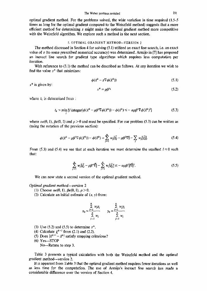
optimal gradient method. For the problems solved, the wide variation in time required (1.5-5 times as long for the optimal gradient compared to the Weiszfeld method) suggests that a more efficient method for determining s might make the optimal gradient method more competitive with the Weiszfeld algorithm. We explore such a method in the next section.

5. OPTIMAL GRADIENT METHOD-VERSION 2

The method discussed in Section 4 for solving (3.1) utilized an exact line search, i.e. an exact value of s (to some prescribed numerical accuracy) was determined. Armijo in [7] has proposed an inexact line search for gradient type algorithms which requires less computation per iteration.

With reference to (3.1) the method can be described as follows. At any iteration we wish to find the value s* that minimizes:

s* is given by: &nk - sV4(P)) (5.1)

s* = pp’k (5.2)

where tk is determined from :

tk = mi: [I integer]4(ffk - @‘v4(ak)) - d(zk) 5 - ~&v~(~k)2] (5.3)

where ~(0, l), @(O, 1) and p > 0 and must be specified. For our problem (5.3) can be written as (using the notation of the previous section):

(5.4)

From (5.3) and (5.4) we see that at each iteration we must determine the smallest 1~ 0 such that:

We can now state a second version of the optimal gradient method.

Optimal gradient method-version 2 (1) Choose (YE(O, l), @(O, l), p > 0. (2) Calculate an initial estimate of (x, y) from:

5 WjXj j=t

i Wjyj

x0=-

i wj

y. = i+-

j=l Z Wj

j=l

(3) Use (5.2) and (5.5) to determine s*. (4) Calculate XL+’ from (2.1) and (2.2). (5) Does (fk+’ - fkJ satisfy stopping criterions? (6) Yes-STOP

No-Return to step 3.

(5.5)

Table 3 presents a typical calculation with both the Weiszfeld method and the optimal gradient method-version 2.

It is apparent from Table 3 that the optimal gradient method requires fewer iterations as well as less time for the computation. The use of Armijo’s inexact line search has made a considerable difference over the version of Section 4.

232 L. CGOPER~~~ I.N.KATz

In Table 4 results are given for 18 randomly generated problems showing the number of iterations for the Weiszfeld method (Iw) and the method of this paper (1,) as well as the CPU time in seconds (CPUw) and (CPUd).

The differences in the CPU times for the two methods, which are given in Table 4, have been analyzed using a Wilcoxon Rank Sum Test. The data are shown in Table 5. The smaller sum is for the negative differences and is T = 6 + 10 + 18 = 34 and it = 18. The critical value for a two-tailed test (a = 0.05) is T = 40. Therfore we reject the null hypothesis. The differences in Tables 4 and 5 indicate that there is a significant difference in the population distributions.

The above results have been obtained with (Y = 0.5, /3 = 0.5, p = 1.0. There are reasons for believing that these are “reasonable” values to use (see [S]). In individual cases, even better results can be obtained with different values of (Y, p, p. However, the values of (Y, /3, p as given above produce an algorithm which is superior to the Weiszfeld method, both in terms of the number of iterations and the time to compute a solution.

6. SUMMARY AND CONCLUSIONS

An optimal gradient method with an inexact line search has been proposed and developed for the solution of the Weber problem. It has been shown that this optimal gradient method converges more rapidly than the Weiszfeld method, which is a gradient method with a non-optimal step size at each iteration. It has also been shown that the new method is faster than the Weiszfeld method on a set of test problems.

Table 3. Sample problem comparison

wj = 3,8,3,7,1,3,9,6,7,5

x. 3

Y. J

89.000 73.000 36.000 89.000 39.000 9.000 14.000 5.000 46.000 12.000 55.000 1.000 53.000 64.000 32.000 57.000 68.000 42.000 63.000 92.000

xk -

Weiszfeld

vk

46.942308

50.153418 50.470247

48.351592

50.705512 50.883581

49.144216

51.021234 51.129692

49.723178

51.216536 51.287007 51.344831 51.392719 51.432688 51.466267 51.494636 51.518717 51.539240 51.556794 51.571852 51.584803 51.595967 51.605608 51.613948 51.621173 51.627441 51.632883 51.637614 51.641729

59.849657

51.538462

60.361209 60.726363

55.727316

60.997635 61.205102

57.873619

61.367348 61.496503

59.090940

61.600814 61.686069 61.756445 61.815022 61.864122 61.905522 61.940607 61.970467 61.995975 62.017835 62.036618 62.052797 62.066760 62.078832 62.089286 62.098349 62.106217 62.113054 62.118999

1775.527415 1744.602952 1734.700436 1730.710150 1728.821295 1727.826614 1727.262579 1726.924672 1726.713455 1726.576921 1726.486252 1726.424706 1726.382167 1726.352322 1726.331120 1726.315898 1726.304873 1726.296826 1726.290915 1726.286549 1726.283308 1726.280894 1726.279089 1726.277734 1726.276716 1726.275949 1726.275369 1726.274930 1726.274598 1726.214346

xk

The Weber problem revisited 233

Table 3. (Con@

Weiszfeld

51.645311 51.648432 51.651152 51.653523 51.655592 51.657398 51.658974 51.660350 51.661552 51.662602 51.663519 51.664321 51.665022 51.665634

Z=

46.942308 49.745193 51.480562 51.254137 51.309246 51.494464 51.486894 51.551031 51.622453 51.649496 51.645684 51.665209 51.662750 51.666010 51.666114 51.667492 51.668635 51.669237

(X,Y) =

CPU =

62.124173 1726.274155 62.128680 1726.274009 62.132606 1726.273898 62.136030 1726.273814 62.139016 1726.273750 62.141622 1726.273701 62.143896 1726.273663 62.145882 1726.273635 62.147616 1726.273613 62.149131 1726.273597 62.150454 1726.273584 62.151610 1726.273574 62.152621 1726.273567 62.153504 1726.273561

1726.274

(51.666, 62 .154)

.3300 seconds

Optimal Gradient (II)

t( = .5, B = .5, P = 1

- 51.528462 59.869555 61.107380 61.430830 61.726074 61.822867 61.977678 61.983694 62.104029 62.114340 62.126719 62.145838 62.150341 62.152767 62.155843 62.155945 62.158688 62.158575

1775.527415 1729.349674 1726.911976 1726.512461 1726.382404 1726.324648 1726.299356 1726.288369 1726.275400 1726.274511 1726.274094 1726.273644 1726.273589 1726.273564 1726.273554 1726.273549 1726.273544 1726.273543

z = 1726.274

(x,y) = (51.669, 62.159)

CPU = .2230 seconds

Table 4.

No.

No. of Iterations

IW

CPUw

(Sec.)

No. of Iterations

IG

CPUG

(Sec.)

3 %i E 0.223 0.117 2: 0:215 0.326 2164 0.266 0.181

sz 0.242 0.170 ;: 0.213 0.196 188 0.566 0.132 23 0.167 0.379

;: 0.203 0.153 :'6 14 0.147 0.141 :54 0.112 0.238 23 0.096 0.236

29 0.204 1; 0.437

:: 0.127 0.119 9 0.082 0.112 20 0.143 11; 0.115 z 0.167 0.368 :z 0.298 0.152

CAMWA Vol. 7, No. S-C

234 L. COOPER and I. N. KAY

Table 5. Test of significance

CPUw CPUG CPu,-CPUG Rank

0.330 0.223 0 1n7 0.135 0.117 0.215 0.181 0.326 0.266 0.242 0.213 0.170 0.196 0.566 0.379

-. __. 0.108 0.034 0.060 0.029 .0.026 0~187

0.132 O.i67 -0.035 0.153 0.147 0.006 0.203 0.141 0.062 0.238 0.236 0.002 0.112 0.096 0.016 0.204 0.437 -0.233 0.127 0.082 0.045 0.119 0.112 0.007 0.143 0.115 0.028 0.167 0.152 0.015 0.368 0.298 0.070

E 9 12 a

176 10

1: 51 18 11 3

z 16

REFERENCES 1. E. Weiszfeld, Sur le point pour lequel la somme des distances de II points don& est minimum. Tohoku Math. J. 43,

335-386 (1937). 2. L. Cooper, Location-allocation problems. Ops. Res. 11,331-343 (l%3). 3. H. W. Kuhn and R. E. Kuenne, An efficient algorithm for the numerical solution of the generalized Weber problem in

spatial economics. J. Reg. Sci. 4, 21-33 (1%2). 4. B. Harris, Personal Communication. 5. 1. Kowalik and M. R. Osborne, Methods for unconstrained optimization problems. American Elsevier, New York (1968). 6. I. N. Katz, Local convergence in Fermat’s problem. Math. Prog. 6,8!9-104 (1974). 7. L. Armijo, Minimization of functions having continuous partial derivatives. Pacific J. Math. 16, 1-3 (l%6). 8. E. Polak, CotnpuWonal Methods in Optimazalion. Academic Press, New York (1971).