The Value of Forever Wild: An Economic Analysis of Land...
20
Agricultural and Resource Economics Review 42/1 (April 2013) 119–138 Copyright 2013 Northeastern Agricultural and Resource Economics Association The Value of Forever Wild: An Economic Analysis of Land Use in the Adirondacks Carrie M. Tuttle and Martin D. Heintzelman The mix of public and private land ownership within the Adirondack Park often leads to conflict between development and conservation interests. We explore the effects of the Adirondack Park Agency’s classifications on property values through hedonic analysis while simultaneously controlling for environmental and recreational amenities. Results show that lands in the park classified for moderate- intensity use sell at a premium of up to 7 percent while lands in more restrictive classes are discounted. There is also evidence that decreasing the impact of humans by one unit increases property values by approximately 2 percent. Key Words: Adirondacks, hedonic pricing model, land use The Adirondack Park is one of our nation’s most interesting experiments in conservation. Comprised of approximately 6.1 million acres, the Adirondack Park is located in northern New York in an area made up of great tracts of forest with thousands of miles of lakefront, rivers, streams, and brooks and 42 peaks that rise more than 4,000 feet above sea level. Part of what makes Adirondack Park unique is the history of its creation through an unusual alliance of merchants, conservationists, the lumber industry, and the wealthy elite in the late nineteenth century. This group of supporters proposed creation of a protected area that was unlike any that had been created before or any that exist now. Today, mostly as it was when first created in 1885, 47 percent of the park is owned by the public and 53 percent by private interests. Public land in the park is protected as “forever wild” by provisions in the New York State Constitution. In addition, though, private land in the park is subject to substantial state-level regulations that restrict its use, limits that extend far beyond typical local zoning ordinances. Of course, a primary rationale for the regulations is protection of the ecosystem and other amenities provided by the wild character of much of the park. These benefits accrue not just to residents of the park but to visitors and others who appreciate perhaps the mere existence of such a “wild” area. This atypical mix of public/private land ownership within a publicly protected state park often leads to conflict between development and conservation interests. Carrie Tuttle is a research assistant professor at the Institute for a Sustainable Environment and Martin Heintzelman is an associate professor in the School of Business and Fredric C. Menz Scholar of Environmental Economics at Clarkson University in Potsdam, New York. Corresponding Author: Martin Heintzelman § School of Business § Clarkson University § Potsdam, New York 13699 § Phone 315.268.6427 § Email mheintze@clarkson.edu. This paper was a selected presentation at the workshop “The Economics of Rural and Agricultural Ecosystem Services” organized by the Northeastern Agricultural and Resource Economics Association (NAREA) in Lowell, Massachusetts, June 12 and 13, 2012. The workshop received financial support from the U.S. Department of Agriculture’s National Institute of Food and Agriculture (Award 2011-67023-30913). The views expressed in this paper are the authors’ and do not necessarily represent the policies or views of the sponsoring agencies.
Transcript of The Value of Forever Wild: An Economic Analysis of Land...

Agricultural and Resource Economics Review 42/1 (April 2013) 119–138Copyright 2013 Northeastern Agricultural and Resource Economics Association
The Value of Forever Wild: An Economic Analysis of Land Use in the AdirondacksCarrie M. Tuttle and Martin D. Heintzelman
The mix of public and private land ownership within the Adirondack Park often leads to conflict between development and conservation interests. We explore the effects of the Adirondack Park Agency’s classifications on property values through hedonic analysis while simultaneously controlling for environmental and recreational amenities. Results show that lands in the park classified for moderate-intensity use sell at a premium of up to 7 percent while lands in more restrictive classes are discounted. There is also evidence that decreasing the impact of humans by one unit increases property values by approximately 2 percent.
Key Words: Adirondacks, hedonic pricing model, land use
The Adirondack Park is one of our nation’s most interesting experiments in conservation. Comprised of approximately 6.1 million acres, the Adirondack Park is located in northern New York in an area made up of great tracts of forest with thousands of miles of lakefront, rivers, streams, and brooks and 42 peaks that rise more than 4,000 feet above sea level. Part of what makes Adirondack Park unique is the history of its creation through an unusual alliance of merchants, conservationists, the lumber industry, and the wealthy elite in the late nineteenth century. This group of supporters proposed creation of a protected area that was unlike any that had been created before or any that exist now. Today, mostly as it was when first created in 1885, 47 percent of the park is owned by the public and 53 percent by private interests. Public land in the park is protected as “forever wild” by provisions in the New York State Constitution. In addition, though, private land in the park is subject to substantial state-level regulations that restrict its use, limits that extend far beyond typical local zoning ordinances. Of course, a primary rationale for the regulations is protection of the ecosystem and other amenities provided by the wild character of much of the park. These benefits accrue not just to residents of the park but to visitors and others who appreciate perhaps the mere existence of such a “wild” area. This atypical mix of public/private land ownership within a publicly protected state park often leads to conflict between development and conservation interests.
Carrie Tuttle is a research assistant professor at the Institute for a Sustainable Environment and Martin Heintzelman is an associate professor in the School of Business and Fredric C. Menz Scholar of Environmental Economics at Clarkson University in Potsdam, New York. Corresponding Author: Martin Heintzelman § School of Business § Clarkson University § Potsdam, New York 13699 § Phone 315.268.6427 § Email [email protected].
This paper was a selected presentation at the workshop “The Economics of Rural and Agricultural Ecosystem Services” organized by the Northeastern Agricultural and Resource Economics Association (NAREA) in Lowell, Massachusetts, June 12 and 13, 2012. The workshop received financial support from the U.S. Department of Agriculture’s National Institute of Food and Agriculture (Award 2011-67023-30913). The views expressed in this paper are the authors’ and do not necessarily represent the policies or views of the sponsoring agencies.

120 April 2013 Agricultural and Resource Economics Review
We develop an econometric model using property sales transactions between 2001 and 2007 in the twelve counties that comprise Adirondack Park to investigate how state land use classifications, corresponding development restrictions, and ecological amenities provided by the regulations affect private property values. The issues we raise are central to the ongoing debate over land use restrictions in the Adirondacks. Many year-round residents of the 103 municipalities located within the park’s border (known as “the blue line”) argue that the land use restrictions stifle economic development and limit employment opportunities. An equally passionate group of conservationists wants to protect and preserve the Adirondack Park and usually opposes any development for fear that the wilderness and biodiversity that make the park unique would be compromised. Still other state taxpayers complain that increases in the amount of public land in New York result in a smaller private tax base to cover the cost of maintaining public land since the state is obligated to pay local property taxes on its public land.
Increased development within the park would inarguably change the Adirondacks. As these debates continue, stakeholders on both sides are searching for information on how the existing land use restrictions have affected the park both economically and environmentally. We provide evidence that the land use restrictions and the amenities provided by wild land do, in fact, impact private property values. In particular, we find that lots designated for moderate-intensity development earn a small price premium over lots with other designations. Lots in areas less impacted by humans (determined through measures such as ecological integrity and invasive species) also generate a significant price premium. In addition, when we limit our sample to properties that are outside the park but near its boundaries, we find a significant premium for being outside the park. This suggests that the regulations, ceteris paribus, negatively impact property values. We also find some significant differences in estimated sales prices related to whether property buyers are local to the Adirondacks or not, which implies that there are two distinct real estate markets within the Adirondack Park. Unexpectedly, it appears that buyers from outside the area are not willing to pay a premium for higher levels of ecological integrity. Other types of human impacts do not exhibit this negative effect.
Literature Review
In general, few studies have measured land conservation values for rural, sparsely populated areas of the United States. One hedonic study of a rural area in Michigan found that proximity to forest land, publically owned land, streams, and national scenic rivers did not impact property values while proximity to lakes and suburban open spaces had a positive impact (White and Leefers 2007). This area of Michigan is similar to the Adirondacks in terms of the abundance of lakes and the population density. Other studies have identified a positive influence on property values from proximity to a national wildlife refuge in Massachusetts (Neumann, Boyle, and Bell 2009), a national forest in Vermont (Phillips 2004), remote agricultural lands with wildlife habitat in Wyoming (Bastian et al. 2002), and recreational ranches with increased greenness in Arizona (Sengupta and Osgood 2003). Sengupta and Osgood (2003) also found that proximity to roads, cities, and neighbors increased sale prices, indicating that isolation may be a disamenity.
Economic Analysis of Land Use in the Adirondacks 121Tuttle and Heintzelman
The hedonic literature associated with valuing open spaces and parks in urban and suburban areas is substantial (Benson, Hansen, and Schwartz 1998, Bolitzer and Netusil 2000, Lutzenhiser and Netusil 2001, Acharya and Bennett 2001, Irwin 2002, Geoghegan 2002, Anderson and West 2006, Cho, Poudyal, and Roberts 2008, Chamblee et al. 2011). There also is a considerable body of work on the impacts of zoning and preservation policies (Maser, Riker, and Rosett 1977, Spalatro and Provencher 2001, Netusil 2005, Heintzelman 2010a, 2010b). However, results for urban and suburban areas are difficult to translate to the Adirondacks given the significant differences in socio-economic, spatial, and property characteristics. The population density for the Adirondack Park is fourteen people per square mile, which is comparable to South Dakota’s (Adirondack Park Regional Assessment Steering Committee 2009).
Finally, a small number of studies relate directly to our goal: broadening our understanding of the value people place on the amenities of biodiversity and wilderness provided by land use regulations and the existence of protected land (Curran 1990, Glennon 2002, Ito, Mitchell, and Driscoll 2002). Glennon and Porter (2005) used a variety of statistical techniques to determine how biological integrity related to major kinds of land use and to quantify the degree to which land management regulation in the Adirondacks had been effective in maintaining biological integrity. The authors concluded that the greatest number of intact bird communities in the Adirondacks were in forests that had not been developed. They also found that the most important variable affecting biotic integrity was distance to roads, which was likely a proxy for more complex processes that measure humans’ impacts on ecosystem health.
Despite the controversial nature of land use regulation in the Adirondacks, few scientific studies have explored the impact of the park’s restrictions on development on private property values. Anderson and Dower (1980) used 471 in-park and 45 out-of-park sales transactions from 1950 through 1976 to estimate yearly rates of price appreciation for each of five land use classifications for private property. They concluded that the Adirondack Land Use and Development Plan (enacted in 1973 by the Adirondack Park Agency) had affected relative prices for private lands. Properties with less restrictive classifications fetched higher prices than properties with tighter restrictions. Another hedonic study of the Adirondack Park used 284 sales transactions for vacant, forested, non-waterfront property that sold between 1971 and 1973 (Vrooman 1978). Vrooman concluded that the value of privately owned property increased $20 per acre when the properties were adjacent to state land and that nonlocal buyers were willing to pay $19.45 more per acre than buyers who had mailing addresses in the same county as the parcel. Banzhaf et al. (2006) performed a contingent valuation survey to assess mean willingness to pay for ecological improvements gained from additional Clean Air Act legislation and determined that, on average, New York State households would pay between $48 and $159 per year to receive ecological benefits in the Adirondack Park from reductions in acid rain.
Methodology
We used a local-area fixed-effects hedonic pricing model to assess the impacts of land use regulation and ecological amenities on private property values in the Adirondack Park. The hedonic pricing method is a common revealed-preference approach to valuing environmental and other amenities. A number
122 April 2013 Agricultural and Resource Economics Review
of empirical issues are common in hedonic modeling, including omitted variable bias, simultaneity, and spatial dependence and autocorrelation (Gujarati and Porter 2010). The local-area fixed-effects approach mitigates these problems.
Numerous variables affect a property, and the availability of data is a limiting factor in hedonic modeling. Researchers are restricted to variables for which they have information and know that many of the characteristics that co-determine the price of a property must be omitted from the model. Omitted variables generate bias when there is correlation between unobserved characteristics and those included in the model. When dealing with omitted variables, the assumed functional form is an important consideration. Traditionally, researchers have focused on log-linear or linear specifications based on Cropper, Deck, and McConnell (1988). Recent additions to the literature indicate, however, that models can use more flexible specifications such as the Box-Cox approach when spatial fixed effects control for omitted variable bias, allowing the models to produce results that are more accurate. In addition, time dummy variables should be incorporated into hedonic models to reduce bias that is similar in magnitude to bias from omitted variables (Kuminoff, Parmeter, and Pope 2010).
Simultaneity also is a common empirical issue in hedonic modeling that, in effect, is similar to omitted variable bias. Simultaneity occurs when one or more independent variables are co-determined with the price of the property. The presence of simultaneity results in a biased estimate of the impact of a given independent variable on the dependent variable. In our case, this would be an issue if higher-valued properties were more likely to receive a preferred land use designation. For example, if wealthy landowners were better able to navigate the regulatory system and consequently relax regulation of their properties, then, all else being equal, higher-value properties would be less intensively regulated, which would hamper interpretation of our results. We have reason to believe, however, that this is not a significant issue in our particular case. In the Adirondacks, private land classifications were established in 1973 by the Adirondack Park Agency’s (APA’s) Land Use and Development Plan, which was authorized by the APA Act of 1971. Among the goals specified in the act was for the plan to classify land within the park and set development restrictions that would recognize “the complementary needs of preservation of the park’s resources and open space character and of the park’s permanent, seasonal, and transient populations for growth and service areas, employment, and a strong economic base.” The property classifications established in the plan dictate compatible uses and restrictions on the intensity of development. The designations have changed little since 1973, and the vast majority of parcels in the park retain their original designations. Consequently, historic rather than contemporary factors determine how the present-day parcels are designated, which greatly limits the probability of simultaneity in our model, which uses data for 2001 through 2007.
Another issue is spatial dependence and spatial correlation in home prices. It is common for the price of a given property to be affected by the price of nearby properties. If we do not control for correlation of dependent variables in the model, the results generated from the regressions will be biased. Spatial autocorrelation is similar to spatial dependence in that both errors relate to the specific location of a given property and the relationship that the price of the property has with prices of neighboring properties. With spatial autocorrelation, the error terms of two observations are correlated because
Economic Analysis of Land Use in the Adirondacks 123Tuttle and Heintzelman
of omitted variables inherent to a spatial process (Gujarati and Porter 2010). Correlation of error terms between variables violates the principal assumption of independence of residuals in econometric modeling.1
Greenstone and Gayer (2009) provided a detailed discussed of how fixed effects analysis works to control potential biases by creating a series of spatial dummy variables for the specified extent of the fixed effect (i.e., census block, block group, municipality, etc.). Bourassa, Cantoni, and Hoesli (2007) showed that this “submarket” approach for spatial issues is preferable to a fully spatial econometric approach using spatial error or lag models. The dummy variables capture characteristics that are similar across the extent of the geographic area. They allow us to incorporate unobservable characteristics of nearby properties that affect the price of the property we are measuring, thus greatly limiting the likelihood of biases. There are tradeoffs to consider when choosing the level for the fixed effects. As the scale of the fixed effects gets smaller, the ability to control for omitted variables and spatial dependence increases, but less variation remains, thus limiting one’s ability to identify marginal effects. In our case, we used census-block fixed effects, which provided a greater number of fixed-effect areas than we could obtain using block groups, towns, or counties. We established the census blocks using topography, the size and spacing of water features, the land survey system, and the extent, age, type, and density of urban and rural development.2 We could not use parcel-level fixed effects due to the small number of parcels that transact more than once in our study period. We also ran the analysis using census-block-group and county-level fixed effects and a model without any fixed effects. The results of those analyses were substantially similar, both in quality and in magnitude, to the results we report here.3
In addition to fixed effects, we used clustered error terms at the census-block level.4 Thus we allowed the error terms to be correlated within census blocks but assumed independence of error terms across census blocks. This approach is akin to a spatial error model in which one assumes that the spatial weighting matrix takes the nearly diagonal form of ones in all entries for observations within the same census block and zeros elsewhere.
As for functional form considerations, we took the advice of Kuminoff, Parmeter, and Pope (2010) and applied a Box-Cox specification. Doing so generated a theta value of 0.015, which supported use of the simpler semi-log approach that we then employed throughout the remainder of the study. Our basic model is represented by
(1) ln pijt = λt + αj + zit β + χij δj + ηjt + ξit
where pijt represents the price of property i in fixed-effects group j at time t, λt represents a set of time-series dummy variables for the month and year of sale, αj represents the census-block fixed effects, zit represents land use variables, χij represents standard property characteristics such as the size of the home and
1 Due to a data limitation, we could not easily test for spatial dependence and autocorrelation. Both, however, are quite common in a hedonic context, which explains increasing use of spatial econometric methods. See, for instance, Anselin and Le Gallo (2006) and Bourassa, Cantoni, and Hoesli (2007).
2 See www.census.gov/geo/www/GARM/Ch11GARM.pdf.3 The full results of these robustness checks are available from the authors.4 This approach simultaneously controls for heteroskedasticity (Wooldridge 2002).

124 April 2013 Agricultural and Resource Economics Review
lot and number of bathrooms, and ηjt and ξit represent the fixed-effects group error and individual error terms, respectively.
Data
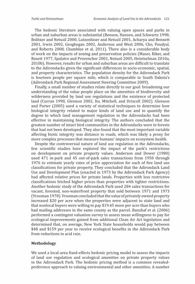
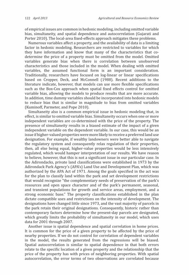
Our data set consisted of real estate transactions for seven years (2001 through 2007) provided by the New York State Office of Real Property Services (NYSORPS).5 Figures 1 and 2 show the locations of transactions within our study area. That data set was combined with detailed parcel and property characteristics, also provided by NYSORPS, allowing us to develop a baseline data set. Table 1 provides a listing of each data set used in the study and its source. Summary statistics for both the the Adirondack Park data set and the blue-line (park boundary) proximity data set are presented in Tables 2 and 3, respectively. We used STATA and ESRI’s ArcView software to combine the data sets and measure the distance from each parcel centroid to certain environmental and cultural amenities, including forests, lakes, and roads. We also included proximity to select North American population centers based on five categories of population size that ranged from 5,000 to 8 million people. Finally, we used the buyers’ zip codes to create dummy variables for buyers located inside the north country region (the counties that make up the Adirondack Park and environs) and buyers located elsewhere.6 We then incorporated other park-specific data to form our final data set. A brief description of the park-specific data follows.
The APA classifies land into 14 categories. Public lands are separated using nine categories that are based on detailed definitions in the agency’s State Land Master Plan (State of New York Adirondack Park Agency and New York State Department of Environmental Conservation 1973). The most restrictive classification is wilderness area, generally a large contiguous tract of state-owned land. Private land holdings make up the balance (53 percent) of the park and are our focus since they are the only properties that transact on a regular basis. The park’s private lands fall into six categories: industrial (0.21 percent), resource management (26 percent), rural (17 percent), low-intensity development (5 percent), moderate-intensity development (2 percent), and hamlet (1 percent). The land use category dictates how dense development on the property can be with hamlets being the least restrictive and resource management being the most restrictive private land category.
Under the hamlet designation (village areas that existed in 1973 plus some then-vacant surrounding land), there is no restriction on building density, and APA permits are required only for structures that exceed 40 feet in height. The next most restrictive category, moderate intensity, restricts development to a 1.3-acre average lot size per parcel.7 This category contains land that surrounds hamlets plus much of the park’s private waterfront property. The
5 We originally included data for 2008 and 2009 as well. However, in response to a reviewer’s suggestion, we tested the effect of eliminating those years because of the real estate crisis at that time. Because inclusion of those years caused significant differences in the results, we decided to eliminate them.
6 North country buyers are from Clinton, Franklin, Fulton, Hamilton, Herkimer, Essex, Lewis, Oneida, Saratoga, St. Lawrence, Warren, or Washington County.
7 A “parcel” in this case refers to property boundaries as they existed in 1973, the year in which the Adirondack Park Land Use and Development Plan was initially completed. Any new construction or subdivision must conform to the density restrictions that applied to the land under the original parcel boundaries.
Economic Analysis of Land Use in the Adirondacks 125Tuttle and Heintzelman
Figure 1. Adirondack Park Property Sales
Figure 2. Property Sales within Five Miles of the Adirondack Park Blue Line
AdirondackParkBoundaryCountyBoundariesPropertySales
AdirondackParkBoundaryCountyBoundariesPropertySales
126 April 2013 Agricultural and Resource Economics Review
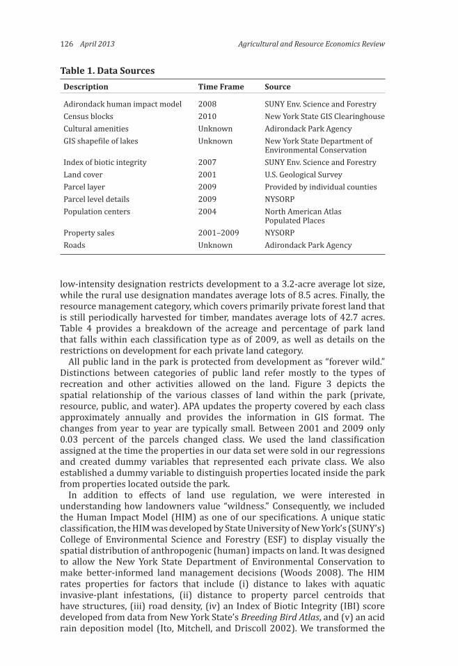
Table 1. Data SourcesDescription Time Frame Source
Adirondack human impact model 2008 SUNY Env. Science and ForestryCensus blocks 2010 New York State GIS ClearinghouseCultural amenities Unknown Adirondack Park AgencyGIS shapefile of lakes Unknown New York State Department of Environmental Conservation Index of biotic integrity 2007 SUNY Env. Science and ForestryLand cover 2001 U.S. Geological SurveyParcel layer 2009 Provided by individual countiesParcel level details 2009 NYSORPPopulation centers 2004 North American Atlas Populated Places Property sales 2001–2009 NYSORPRoads Unknown Adirondack Park Agency
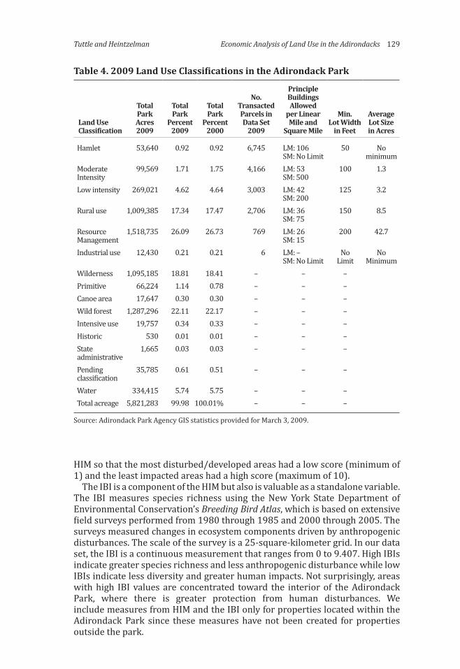
low-intensity designation restricts development to a 3.2-acre average lot size, while the rural use designation mandates average lots of 8.5 acres. Finally, the resource management category, which covers primarily private forest land that is still periodically harvested for timber, mandates average lots of 42.7 acres. Table 4 provides a breakdown of the acreage and percentage of park land that falls within each classification type as of 2009, as well as details on the restrictions on development for each private land category.
All public land in the park is protected from development as “forever wild.” Distinctions between categories of public land refer mostly to the types of recreation and other activities allowed on the land. Figure 3 depicts the spatial relationship of the various classes of land within the park (private, resource, public, and water). APA updates the property covered by each class approximately annually and provides the information in GIS format. The changes from year to year are typically small. Between 2001 and 2009 only 0.03 percent of the parcels changed class. We used the land classification assigned at the time the properties in our data set were sold in our regressions and created dummy variables that represented each private class. We also established a dummy variable to distinguish properties located inside the park from properties located outside the park.
In addition to effects of land use regulation, we were interested in understanding how landowners value “wildness.” Consequently, we included the Human Impact Model (HIM) as one of our specifications. A unique static classification, the HIM was developed by State University of New York’s (SUNY’s) College of Environmental Science and Forestry (ESF) to display visually the spatial distribution of anthropogenic (human) impacts on land. It was designed to allow the New York State Department of Environmental Conservation to make better-informed land management decisions (Woods 2008). The HIM rates properties for factors that include (i) distance to lakes with aquatic invasive-plant infestations, (ii) distance to property parcel centroids that have structures, (iii) road density, (iv) an Index of Biotic Integrity (IBI) score developed from data from New York State’s Breeding Bird Atlas, and (v) an acid rain deposition model (Ito, Mitchell, and Driscoll 2002). We transformed the

Economic Analysis of Land Use in the Adirondacks 127Tuttle and Heintzelman
Table 2. Select Summary Statistics for the Adirondack ParkVariable Mean Std. Dev. Min Max
Sale price (dollars) $179,526 $260,214 $10,000 $6,250,000Personal property ($10,000) $0.04 $0.68 $0.00 $50.00
Land Use Characteristics
APA land class hamlet 0.36 0.48 0 1APA land class moderate intensity 0.25 0.43 0 1APA land class low intensity 0.17 0.38 0 1APA land class rural 0.16 0.37 0 1APA land class resource management 0.05 0.21 0 1Human Impact Model 1.17 2.37 0 10Index of Biotic Integrity 3.16 1.61 0.23 9.41
Buyer Characteristics
Buyer out of north country 0.43 0.50 0 1
Proximity Characteristics
Distance to blue line (miles) 12.70 10.38 0.00 42.22Distance to nearest forest (miles) 2.81 4.50 0.01 23.45Distance to nearest lake (miles) 1.07 1.85 0.00 25.31Size of nearest lake (acres) 6,837.95 12,208.24 0.67 54,971.63Waterfront 0.16 0.36 0 1Distance to nearest road (feet) 1,813.20 3,332.75 0.00 42,823.13Road distance to nearest recreation (miles) 5.35 4.02 0.03 24.85Distance to population center 1 46.55 23.48 0.16 110.50Distance to population center 2 30.82 12.50 1.59 66.72Distance to population center 3 103.70 16.29 23.46 133.56Distance to population center 4 121.57 30.33 46.60 196.69Distance to population center 5 219.90 30.25 151.54 301.20
Structure/Parcel Characteristics
Building age (years) 38.72 31.56 2 231Lot size (acres) 6.14 71.91 0.01 7,421.2Living area (square feet) 1522 749 1 9,032Bedrooms 2.83 1.05 0 17Fireplaces 0.40 0.61 0 8Full baths 1.51 0.76 0 9Seasonal 0.14 0.35 0 1Estate 0.00 0.03 0 1Agricultural 0.00 0.05 0 1Multi-family year round 0.03 0.16 0 1Mobile home 0.00 0.05 0 1Other property class 0.01 0.12 0 1
Note: 13,554 observations.

128 April 2013 Agricultural and Resource Economics Review
Table 3. Select Summary Statistics for One, Three, and Five Mile Buffer from Blue LineVariable One Mile Three Miles Five Miles
Sale price (dollars) $141,172 $124,920 $132,792Personal property ($10,000) $0.00 $0.01 $0.01
Land Use Characteristics
APA land class hamlet 0.58 0.13 0.10APA land class moderate intensity 0.17 0.08 0.08APA land class low intensity 0.11 0.05 0.04APA land class rural 0.05 0.05 0.04APA land class resource management 0.07 0.01 0.01Out of park 0.56 0.67 0.73
Buyer Characteristics
Buyer out of north country 0.25 0.23 0.21
Proximity Characteristics
Distance to blue line (miles) 0.52 1.59 2.60Distance to nearest forest (miles) 1.76 2.04 1.84Distance to nearest lake (miles) 1.61 1.79 2.02Size of nearest lake (acres) 5,003 5,147 4,419Waterfront 0.06 0.06 0.05Distance to nearest road (feet) 1195.71 753.80 591.17Road distance to nearest recreation (miles) 7.01 7.44 8.20Distance to population center 1 69.34 68.61 68.49Distance to population center 2 18.93 20.13 19.09Distance to population center 3 96.72 95.76 94.90Distance to population center 4 144.45 142.56 140.91Distance to population center 5 197.29 199.77 201.38
Structure/Parcel Characteristics
Building age (years) 36.13 42.11 47.08Lot size (acres) 5.25 4.60 4.29Living area (square feet) 1,634.53 1,646.47 1,621.37Bedrooms 2.95 3.02 3.05Fireplaces 0.39 0.39 0.35Full baths 1.50 1.51 1.49Seasonal 0.10 0.08 0.07Estate 0.00 0.00 0.00Agricultural 0.00 0.00 0.00Multi-family year round 0.03 0.06 0.08Mobile home 0.00 0.00 0.00Other property class 0.01 0.01 0.01
Observations 2,952 9,656 16,903
Economic Analysis of Land Use in the Adirondacks 129Tuttle and Heintzelman
HIM so that the most disturbed/developed areas had a low score (minimum of 1) and the least impacted areas had a high score (maximum of 10).
The IBI is a component of the HIM but also is valuable as a standalone variable. The IBI measures species richness using the New York State Department of Environmental Conservation’s Breeding Bird Atlas, which is based on extensive field surveys performed from 1980 through 1985 and 2000 through 2005. The surveys measured changes in ecosystem components driven by anthropogenic disturbances. The scale of the survey is a 25-square-kilometer grid. In our data set, the IBI is a continuous measurement that ranges from 0 to 9.407. High IBIs indicate greater species richness and less anthropogenic disturbance while low IBIs indicate less diversity and greater human impacts. Not surprisingly, areas with high IBI values are concentrated toward the interior of the Adirondack Park, where there is greater protection from human disturbances. We include measures from HIM and the IBI only for properties located within the Adirondack Park since these measures have not been created for properties outside the park.
Table 4. 2009 Land Use Classifications in the Adirondack Park
Land Use Classification
Total Park Acres 2009
Total Park
Percent 2009
Total Park
Percent 2000
No. Transacted Parcels in Data Set
2009
Principle Buildings Allowed
per Linear Mile and
Square Mile
Min. Lot Width
in Feet
Average Lot Size in Acres
Hamlet 53,640 0.92 0.92 6,745 LM: 106 50 No SM: No Limit minimumModerate 99,569 1.71 1.75 4,166 LM: 53 100 1.3 Intensity SM: 500Low intensity 269,021 4.62 4.64 3,003 LM: 42 125 3.2 SM: 200Rural use 1,009,385 17.34 17.47 2,706 LM: 36 150 8.5 SM: 75Resource 1,518,735 26.09 26.73 769 LM: 26 200 42.7 Management SM: 15Industrial use 12,430 0.21 0.21 6 LM: – No No SM: No Limit Limit MinimumWilderness 1,095,185 18.81 18.41 – – –Primitive 66,224 1.14 0.78 – – –Canoe area 17,647 0.30 0.30 – – –Wild forest 1,287,296 22.11 22.17 – – –Intensive use 19,757 0.34 0.33 – – –Historic 530 0.01 0.01 – – –State 1,665 0.03 0.03 – – – administrativePending 35,785 0.61 0.51 – – – classificationWater 334,415 5.74 5.75 – – –Total acreage 5,821,283 99.98 100.01% – – –
Source: Adirondack Park Agency GIS statistics provided for March 3, 2009.

130 April 2013 Agricultural and Resource Economics Review
Results
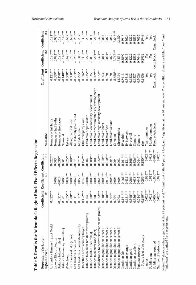
Table 5 presents results for our regressions using only sales transactions that occurred within the park’s boundaries. We report three specifications: HIM only, IBI only, and HIM plus IBI. These two measures are correlated (correlation coefficient of 0.5176), as we would expect, since the IBI is a component of the HIM so we report results for all three specifications.
Our results indicate that landowners prefer properties classified as moderate-intensity to properties designated as hamlet or low-intensity development. In particular, lots designated as moderate-intensity were sold for between 5 percent and 7 percent more, on average, than homes with other designations. Being inside of a hamlet had a negative but not statistically significant effect relative to the other land use categories. This preference was evident despite our controlling for distance to roads, villages, and lakes and for waterfront status and broader human impact/ecological integrity measures. These controls were important since moderate-intensity zones were more likely to involve waterfront properties and to be on the outskirts of hamlets.
Also, and as expected, there was a strong price premium generally for sites on the water and sites that were close to a lake. In addition, the premium was
Figure 3. Adirondack Park Land Use Classifications
AdirondackParkBoundaryCountyBoundaries
PrivateResourcePublicWater
APA 2009 Land Classes
Economic Analysis of Land Use in the Adirondacks 131Tuttle and Heintzelman
Tabl
e 5.
Res
ults
for
Adir
onda
ck R
egio
n Bl
ock
Fixe
d Ef
fect
s Re
gres
sion
Dep
ende
nt V
aria
ble:
Co
effic
ient
Coe
ffici
ent
Coef
ficie
nt
Co
effic
ient
Coe
ffici
ent
Coef
ficie
nt
ln(S
ale
Pric
e)
R1
R2
R3
Vari
able
R1
R2
R3
Adiro
ndac
k Hu
man
Impa
ct M
odel
0.
022*
**
0.
022*
**
Num
ber o
f ful
l bat
hs
0.12
1***
0.
120*
**
0.12
1***
Inde
x of B
iotic
Inte
grity
0.00
9 0.
003
Num
ber o
f hal
f bat
hs
0.08
9***
0.
091*
**
0.08
9***
Dist
ance
to la
ke (m
iles)
–0
.031
**
–0.0
14
–0.0
30**
Nu
mbe
r of f
irepl
aces
0.
198*
**
0.19
9***
0.
198*
**Di
stan
ce to
lake
(squ
are m
iles)
0.
001
0.00
0 0.
001
Seas
onal
–0
.148
***
–0.1
45**
* –0
.149
***
Wat
erfro
nt
0.82
5***
0.
832*
**
0.82
5***
Es
tate
0.
608*
**
0.62
9***
0.
607*
**Si
ze o
f nea
rest
lake
(acr
es)
0.00
0***
0.
000*
**
0.00
0***
Al
l agr
icultu
ral u
ses
0.68
0***
0.
705*
**
0.68
2***
APA
land
clas
s ham
let
–0.0
11
–0.0
40
–0.0
11
Mul
ti-fa
mily
year
roun
d –0
.253
***
–0.2
58**
* –0
.253
***
APA
land
clas
s mod
erat
e int
ensit
y 0.
071*
* 0.
053*
0.
071*
* M
obile
hom
e –0
.295
* –0
.319
**
–0.2
97*
Othe
r tha
n no
rth
coun
try b
uyer
0.
152*
**
0.14
9***
0.
152*
**
Othe
r pro
pert
y cla
ss
0.33
6***
0.
332*
**
0.33
6***
Dist
ance
to n
eare
st N
Y st
ate f
ores
t (m
iles)
–0
.004
–0
.004
–0
.004
La
nd co
ver o
pen
wat
er
0.23
5***
0.
229*
**
0.23
3***
Dist
ance
to b
lue l
ine (
mile
s)
0.00
8***
0.
008*
**
0.00
8***
La
nd co
ver l
ow in
tens
ity d
evel
opm
ent
–0.0
35
–0.0
30
–0.0
34Di
stan
ce to
nea
rest
road
(fee
t) –0
.000
–0
.000
–0
.000
La
nd co
ver m
ediu
m in
tens
ity d
evel
opm
ent
–0.2
09**
* –0
.204
***
–0.2
08**
*Ro
ad d
istan
ce to
nea
rest
recr
eatio
n sit
e (m
iles)
–0.
022*
**
–0.0
23**
* –0
.022
***
Land
cove
r hig
h in
tens
ity d
evel
opm
ent
–0.3
22**
–0
.321
**
–0.3
20**
Dist
ance
to p
opul
atio
n ce
nter
1
–0.0
10**
* –0
.009
***
–0.0
10**
* La
nd co
ver f
ores
t –0
.003
–0
.011
–0
.004
Dist
ance
to p
opul
atio
n ce
nter
2
–0.0
10**
* –0
.010
***
–0.0
10**
* La
nd co
ver f
ield
0.
070
0.09
1*
0.07
0Di
stan
ce to
pop
ulat
ion
cent
er 3
0.
004*
* 0.
003*
* 0.
004*
* La
nd co
ver w
etla
nd
0.07
0 0.
076
0.06
9Di
stan
ce to
pop
ulat
ion
cent
er 4
0.
004
0.00
4 0.
004
Cons
tant
8.
658*
**
8.76
2***
8.
646*
**Di
stan
ce to
pop
ulat
ion
cent
er 5
–0
.003
–0
.004
–0
.003
Ob
serv
atio
ns
13,5
54
13,5
54
13,5
54Co
nditi
on fa
ir 0.
161*
**
0.16
1***
0.
161*
**
R2 with
in
0.39
13
0.38
97
0.39
13Co
nditi
on av
erag
e 0.
431*
**
0.43
1***
0.
431*
**
R2 bet
wee
n 0.
5618
0.
5618
0.
5624
Cond
ition
good
0.
368*
**
0.36
6***
0.
368*
**
R2 ove
rall
0.43
32
0.43
22
0.43
32Co
nditi
on ex
celle
nt
0.63
6***
0.
638*
**
0.63
6***
Si
gma_
u 0.
4537
0.
4538
0.
4535
Pers
onal
pro
pert
y 0.
044*
**
0.04
5***
0.
044*
**
Sigm
a_e
0.70
36
0.70
46
0.70
37ln
Squa
re fe
et o
f str
uctu
re
0.28
0***
0.
286*
**
0.28
0***
rh
o 0.
2936
0.
2932
0.
2943
ln A
cres
0.
026*
**
0.02
6**
0.02
6***
Ye
ar d
umm
ies
Yes
Yes
Yes
Build
ing a
ge
0.01
2***
0.
012*
**
0.01
2***
M
onth
dum
mie
s Ye
s Ye
s Ye
sBu
ildin
g age
squa
red
–0.0
00**
* –0
.000
***
–0.0
00**
* Fi
xed
effe
cts l
evel
Ce
ns. b
lock
Ce
ns. b
lock
Ce
ns. b
lock
Num
ber o
f bed
room
s 0.
020*
0.
021*
* 0.
020*
Not
es: *
** d
enot
es v
alue
s sig
nific
ant a
t the
99
perc
ent l
evel
, ** s
igni
fican
t at t
he 9
5 pe
rcen
t lev
el, a
nd *
sign
ifica
nt a
t the
90
perc
ent l
evel
. The
cond
ition
dum
my
vari
able
s “po
or” a
nd
“unk
now
n” a
re o
mitt
ed fr
om re
gres
sion
s.

132 April 2013 Agricultural and Resource Economics Review
greater when the nearby lake was larger. Other proximity variables’ coefficients also were significant, including locations close to wild forests, recreation sites, and the park’s border. We also found a preference for proximity to small and medium population centers and an aversion to proximity to more populated areas. The structural and land use variables were all as we expected.
Lower levels of human impact, as modeled by the HIM, had a positive and significant impact on property values while the IBI did not have a significant effect. Because the HIM and IBI measures are indices, it is difficult to interpret the magnitude of these effects beyond noting that a one-unit increase in the HIM results in a 2.2 percent increase in sales prices. Obviously, this suggests that the extent of local human impact affects property values and that less impacted regions are preferred.
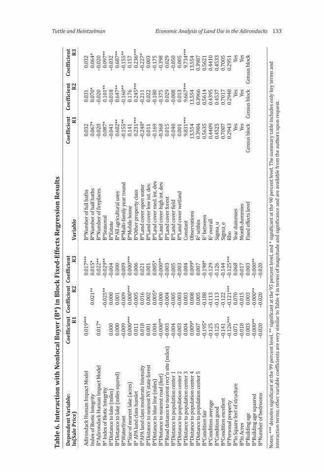
Interestingly, buyers from outside of the north country region paid a premium of as much as 15 percent for properties when all other variables were equal.8 There are a number of possible explanations for this result. Our model may have omitted variables for characteristics preferred by nonlocal buyers even though we accounted for housing quality using assessment data. Such unobserved characteristics could command a premium from the nonlocal market segment. The premium also could be related to whether purchases represent primary residences or second homes. In that case, we could be looking at two separate real estate markets. To answer that question, we ran models corresponding to the ones presented in Table 5, which interact the other-buyer category with each of the explanatory variables. Selected results from that analysis are presented in Table 6. Some of the coefficients from that analysis were significant, suggesting that there are separate markets for local and nonlocal buyers.
In particular, nonlocal buyers pay a premium for property on or near a large lake, although the interaction effect with the waterfront dummy was not significant. Nonlocal buyers also paid a premium for being close to roads and for seasonal9 properties. The interacted results indicate that nonlocal buyers do not favor lower-quality homes and prefer homes that are not especially old given the negative and significant coefficient on the interacted quadratic age term.
Regarding measures of ecological integrity and human impact, both local and nonlocal buyers paid a premium for properties less affected by human activities and for higher levels of biotic integrity. For nonlocal buyers, however, nearly all of the positive impact of biotic integrity was negated with the interaction term. This suggests that ecosystem services receive a larger premium from local buyers than from nonlocal buyers, a surprising result. However, it may indicate a relative preference among nonlocal buyers for easy access to services that are provided only in relatively developed areas, an element that may not be fully captured by our other variables.
8 We initially established four categories of buyers: (i) downstate buyers, (ii) north country buyers, (iii) other New York State buyers, and (iv) out-of-state buyers. We then aggregated all of the categories other than north country into one category so the regressions would be more concise.
9 A seasonal property denotes a parcel with a structure that does not have a heating system or potable water/septic service that would allow people to reside there when the temperatures drop below freezing.
Economic Analysis of Land Use in the Adirondacks 133Tuttle and Heintzelman
Tabl
e 6.
Inte
ract
ion
wit
h N
onlo
cal B
uyer
(B*)
in B
lock
Fix
ed-E
ffect
s Re
gres
sion
Res
ults
Dep
ende
nt V
aria
ble:
Co
effic
ient
Coe
ffici
ent
Coef
ficie
nt
Co
effic
ient
Co
effic
ient
Co
effic
ient
ln
(Sal
e Pr
ice)
R1
R2
R3
Va
riab
le
R1
R2
R3
Adiro
ndac
k Hu
man
Impa
ct M
odel
0.
019*
**
0.
017*
**
B*Nu
mbe
r of f
ull b
aths
0.
032
0.03
1 0.
032
Inde
x of B
iotic
Inte
grity
0.02
1**
0.01
5*
B*Nu
mbe
r of h
alf b
aths
0.
067*
0.
070*
0.
064*
B*Ad
irond
ack
Hum
an Im
pact
Mod
el
0.01
7*
0.
022*
* B*
Num
ber o
f fire
plac
es
–0.0
20
–0.0
20
–0.0
20B*
Inde
x of B
iotic
Inte
grity
–0.0
25**
–0
.029
**
B*Se
ason
al
0.08
7*
0.10
1**
0.09
7**
B*Di
stan
ce to
lake
(mile
s)
0.00
0 0.
000
–0.0
04
B*Es
tate
–0
.041
–0
.018
–0
.032
B*Di
stan
ce to
lake
(mile
s squ
red)
0.
000
0.00
1 0.
000
B*Al
l agr
icultu
ral u
ses
0.68
2**
0.64
7**
0.68
7**
B*W
ater
front
–0
.009
–0
.009
–0
.009
B*
Mul
ti-fa
mily
year
roun
d –0
.155
**
–0.1
60**
–0
.155
**B*
Size
of n
eare
st la
ke (a
cres
) 0.
000*
**
0.00
0***
0.
000*
**
B*M
obile
hom
e 0.
141
0.17
6 0.
157
B* A
PA la
nd cl
ass h
amle
t 0.
011
–0.0
05
0.00
6 B*
Othe
r pro
pert
y cla
ss
0.23
1***
0.
245*
**
0.23
6***
B*AP
A la
nd cl
ass m
oder
ate I
nten
sity
0.01
8 0.
016
0.02
1 B*
Land
cove
r ope
n w
ater
–0
.248
* –0
.211
–0
.227
*B*
Dist
ance
to n
eare
st N
Y st
ate f
ores
t 0.
001
0.00
2 0.
001
B*La
nd co
ver l
ow in
t. de
v. 0.
011
0.02
2 0.
003
B*Di
stan
ce to
blu
e lin
e (m
iles)
0.
004
0.00
5*
0.00
5*
B*La
nd co
ver m
ed. in
t. de
v. –0
.169
–0
.180
–0
.175
B*Di
stan
ce to
nea
rest
road
(fee
t) –0
.000
**
–0.0
00
–0.0
00**
B*
Land
cove
r hig
h in
t. de
v. –0
.368
–0
.375
–0
.398
B*Ro
ad d
istan
ce to
nea
rest
recr
’n si
te (m
iles)
–0
.003
–0
.004
–0
.003
B*
Land
cove
r for
est
0.01
5 0.
029
0.02
9B*
Dist
ance
to p
opul
atio
n ce
nter
1
–0.0
04
–0.0
05
–0.0
05
B*La
nd co
ver f
ield
–0
.040
–0
.008
–0
.050
B*Di
stan
ce to
pop
ulat
ion
cent
er 2
–0
.003
–0
.003
–0
.003
B*
Land
cove
r wet
land
0.
001
0.01
3 0.
005
B*Di
stan
ce to
pop
ulat
ion
cent
er 3
0.
004
0.00
3 0.
004
Cons
tant
9.
831*
**
9.66
7***
9.
734*
**B*
Dist
ance
to p
opul
atio
n ce
nter
4
0.00
9*
0.00
8 0.
009*
Ob
serv
atio
ns
13,5
54
13,5
54
13,5
54B*
Dist
ance
to p
opul
atio
n ce
nter
5
0.00
7 0.
005
0.00
7 R2 w
ithin
0.
3984
0.
3966
0.
3987
B*Co
nditi
on fa
ir –0
.195
* –0
.188
–0
.198
* R2 b
etw
een
0.56
35
0.56
14
0.56
21B*
Cond
ition
aver
age
–0.1
25
–0.1
13
–0.1
29
R2 ove
rall
0.44
09
0.43
95
0.44
10B*
Cond
ition
good
–0
.125
–0
.113
–0
.126
Si
gma_
u 0.
4525
0.
4537
0.
4533
B*Co
nditi
on ex
celle
nt
–0.1
41
–0.1
22
–0.1
44
Sigm
a_e
0.70
07
0.70
17
0.70
05B*
Pers
onal
pro
pert
y –0
.126
***
–0.1
21**
* –0
.125
***
Rho
0.29
43
0.29
48
0.29
51B*
ln Sq
uare
feet
of s
truc
ture
0.
071
0.07
0 0.
068
Year
dum
mie
s Ye
s Ye
s Ye
sB*
ln A
cres
–0
.018
–0
.015
–0
.017
M
onth
dum
mie
s Ye
s Ye
s Ye
sB*
Build
ing a
ge
0.00
3 0.
003
0.00
3 Fi
xed
effe
cts l
evel
Ce
nsus
blo
ck
Cens
us b
lock
Ce
nsus
blo
ckB*
Build
ing a
ge sq
uare
d –0
.000
**
–0.0
00**
–0
.000
**B*
Num
ber o
f bed
room
s –0
.020
–0
.020
–0
.020
Not
es: *
** d
enot
es si
gnifi
cant
at t
he 9
9 pe
rcen
t lev
el, *
* sig
nific
ant a
t the
95
perc
ent l
evel
, and
* si
gnifi
cant
at t
he 9
0 pe
rcen
t lev
el. T
he su
mm
ary
tabl
e in
clud
es o
nly
key
term
s and
in
tera
ctio
n te
rms;
oth
er v
aria
ble
coef
ficie
nts a
re v
ery
sim
ilar t
o Ta
ble
4 in
term
s of m
agni
tude
and
sign
ifica
nce
and
are
avai
labl
e fr
om th
e au
thor
s upo
n re
ques
t.

134 April 2013 Agricultural and Resource Economics Review
Tabl
e 7.
Blu
e Li
ne B
lock
Fix
ed E
ffect
s Re
gres
sion
Res
ults
Dep
ende
nt V
aria
ble:
Co
effic
ient
Coe
ffici
ent
Coef
ficie
nt
Co
effic
ient
Co
effic
ient
Co
effic
ient
ln
(Sal
e Pr
ice)
1
Mile
3
Mile
s 5
Mile
s Va
riab
le
1 M
ile
3 M
iles
5 M
iles
Outs
ide A
diro
ndac
k Pa
rk
0.14
6***
0.
138*
**
0.13
1***
Nu
mbe
r of h
alf b
aths
0.
136*
**
0.10
2***
0.
095*
**Di
stan
ce to
lake
(mile
s)
0.03
4 –0
.021
–0
.037
***
Num
ber o
f fire
plac
es
0.14
1***
0.
168*
**
0.20
2***
Dist
ance
to la
ke (m
iles s
quar
ed)
–0.0
02
0.00
1 0.
002*
* Se
ason
al
–0.1
50**
–0
.171
***
–0.1
52**
*W
ater
front
0.
623*
**
0.71
5***
0.
830*
**
Esta
te
– –0
.079
0.
486*
*Si
ze o
f nea
rest
lake
(acr
es)
–0.0
00**
0.
000
0.00
0**
All a
gricu
ltura
l use
s 0.
266
0.73
6***
0.
700*
**Di
stan
ce to
nea
rest
fore
st (m
iles)
0.
017*
0.
008
–0.0
15**
* M
ulti-
fam
ily ye
ar ro
und
–0.3
30**
* –0
.358
***
–0.3
15**
*Di
stan
ce to
nea
rest
road
(fee
t) 0.
000*
* 0.
000*
**
0.00
0***
M
obile
hom
e –0
.356
* 0.
389*
**
–0.4
62**
*Ro
ad d
istan
ce to
nea
rest
recr
eatio
n sit
e (m
iles)
–0.
039*
**
–0.0
23**
* –0
.007
**
Othe
r pro
pert
y cla
ss
0.15
2*
0.11
5 0.
102*
Dist
ance
to p
opul
atio
n ce
nter
1
–0.0
13
–0.0
22**
* –0
.017
***
Land
cove
r ope
n w
ater
–0
.181
0.
016
0.03
4Di
stan
ce to
pop
ulat
ion
cent
er 2
–0
.010
**
–0.0
18**
* –0
.021
***
Land
cove
r low
int.
dev.
0.06
0 –0
.030
–0
.044
**Di
stan
ce to
pop
ulat
ion
cent
er 3
–0
.005
–0
.003
0.
009*
**
Land
cove
r med
. int.
dev.
–0.2
45**
–0
.373
***
–0.3
25**
*Di
stan
ce to
pop
ulat
ion
cent
er 4
–0
.012
–0
.002
0.
011*
**
Land
cove
r hig
h in
t. de
v. –0
.508
***
–0.2
22
–0.1
23Di
stan
ce to
pop
ulat
ion
cent
er 5
–0
.021
**
–0.0
14**
* 0.
002
Land
cove
r for
est
–0.0
39
–0.0
61
–0.0
69**
Cond
ition
fair
0.19
8*
0.19
3***
0.
178*
**
Land
cove
r fie
ld
0.05
1 0.
060
0.00
5Co
nditi
on av
erag
e 0.
487*
**
0.44
7***
0.
376*
**
Land
cove
r wet
land
0.
031
0.06
5 0.
054
Cond
ition
good
0.
374*
**
0.51
7***
0.
382*
**
Cons
tant
15
.630
***
13.4
53**
* 7.
304*
**Co
nditi
on ex
celle
nt
0.25
0 0.
400
0.74
8**
Obse
rvat
ions
2,
952
9,65
6 16
,903
Pers
onal
pro
pert
y 0.
117*
**
0.02
7 0.
033*
**
R2 with
in
0.31
97
0.35
36
0.36
34ln
Squa
re fe
et o
f str
uctu
re
0.30
3***
0.
310*
**
0.28
2***
R2 b
etw
een
0.54
08
0.53
09
0.50
44ln
Acr
es
0.04
1**
0.03
6***
0.
019*
* R2 o
vera
ll 0.
3981
0.
4146
0.
4080
Buye
r dow
nsta
te
0.06
5 0.
063*
0.
066*
* Si
gma_
u 0.
4840
0.
4414
0.
4450
Buye
r New
York
Stat
e oth
er
0.08
5 0.
013
–0.0
19
Sigm
a_e
0.65
18
0.63
86
0.63
99Bu
yer o
ut o
f sta
te
0.01
4 0.
032
0.03
2*
rho
0.35
55
0.32
32
0.33
09Bu
ildin
g age
0.
007*
**
0.00
7***
–0
.000
Ye
ar d
umm
ies
Yes
Yes
Yes
Build
ing a
ge sq
uare
d –0
.000
***
–0.0
00**
* 0.
000
Mon
th d
umm
ies
Yes
Yes
Yes
Num
ber o
f bed
room
s 0.
033*
0.
025*
* 0.
034*
**
Fixe
d ef
fect
s lev
el
Cens
us b
lock
Ce
nsus
blo
ck
Cens
us b
lock
Num
ber o
f ful
l bat
hs
0.07
7**
0.07
6***
0.
061*
**
Not
es: *
** d
enot
es si
gnifi
cant
at t
he 9
9 pe
rcen
t lev
el, *
* sig
nific
ant a
t the
95
perc
ent l
evel
, and
* si
gnifi
cant
at t
he 9
0 pe
rcen
t lev
el

Economic Analysis of Land Use in the Adirondacks 135Tuttle and Heintzelman
Finally, we ran a series of regressions that focused on properties near the border of the park. In this case, we could not include HIM and IBI variables since those were not measured for properties outside the park. Also, we omitted the land use categories since there were no corresponding categorizations outside of the blue line. We ran these regressions three times to cover properties within one mile, three miles, and five miles of the border while still employing a census-block fixed-effects specification. The results are summarized in Table 7.
Across the board, most of the results for the out-of-park properties are very similar to the results for the in-park sample. Interestingly, in all three regressions there was a significant price premium of 13–14 percent for properties outside the park. For areas near the park border, then, the land use regulations controlling properties inside the park have a negative impact on property values. Along the border, where many of the amenities provided by the park are close by, property owners prefer being outside of the park and unregulated to being inside the park and subject to its more challenging regulatory regime.
Conclusions
Our results indicate that land classifications, ecological integrity, and ecosystem services play significant roles in determining property values. Both the lack of restrictions associated with a hamlet designation and the more stringent restrictions that come with low-intensity and rural classifications reduce the value of property relative to the moderate-intensity designation. It follows that additional development restrictions for hamlet areas could improve property values while additional restrictions on other classes of land could reduce the value of those properties. However, one must be cautious in deriving large-scale policy prescriptions based on these results because of the complex relationship between land use restrictions and ecological integrity.
Our results indicate that buyers prefer a delicate balance of proximity to the amenities found in small population centers and being close to forests and lakes. Since the HIM has a stronger impact on property values than the IBI, it is likely that other components of the HIM (i.e., proximity to lakes infected by invasive species, potential for acid rain, proximity to other parcels that have structures, and road density) play a significant role. This conclusion is consistent with prior studies that found that the presence of invasive species in the nearest lake decreased property values by as much as 9 percent and that potential for acid rain was a significant factor affecting property values in the Adirondack Park (Tuttle and Heintzelman 2013).
Our analysis of the border region shows that there is a significant premium for properties lying just outside the park where owners can take advantage of many of the amenities provided by the park and its regulation without being subject to that regulation. This result conflicts with some earlier studies (Glaeser, Gyourko, and Saks 2005) that showed that tighter land use regulations increased property values by restricting the supply of housing. However, the results were anticipated in our case since supply is limited within the park but not outside it. Consequently, development may shift from inside the park to outside. And while regulation in the park may restrict development options, many building lots are still available in the park.
The Adirondack Park faces many challenges in the years ahead, one of which is increasing development of private land. At full build-out for private land,
136 April 2013 Agricultural and Resource Economics Review
more than 400,000 structures will have been added.10 Between 1967 and 1987, about 19,000 new single family homes were constructed. Today, about 1,000 new structures are built each year. Much of this development is occurring along the shorelines of lakes and rivers and most of it is in areas zoned as hamlet, low-intensity, and moderate-intensity use. As private development increases, the degree of human impact will rise and biotic integrity will decline. Our results confirm that park homeowners prefer a moderate level of development and regulation for themselves and their neighbors. They also prefer to be close to areas where human impacts are relatively minor but not too far away from small population centers. Some critics argue that increased development of this type threatens the very character of the park (Glennon 2009). Policymakers will be faced with a tough decision: whether to increase the amount of land held, and thus protected, by the state or to allow additional development in potentially sensitive environmental areas. Their decisions will have lasting consequences not only for private land values but for the future character of the park.
The value of forever-wild wilderness will continue to be questioned well into the future as park stakeholders try to balance their short-term needs and wants with the aims of conservation. By developing a broader understanding of the value of natural amenities and the effect of land use restrictions on property values, we can begin to consider the implications of potential policy changes in a more holistic manner so that sustainable decisions can be made that will benefit not only current park stakeholders but future generations of Adirondack residents and visitors.
References
Acharya, G., and L.L. Bennett. 2001. “Valuing Open Space and Land-use Patterns in Urban Watershed.” Journal of Real Estate Finance and Economics 22(2/3): 221–237.
Adirondack Park Regional Assessment Steering Committee. 2009. “Adirondack Park Regional Assessment Report.” Available at http://aatvny.org/content /Generic/View/1:field=documents;/content/Documents/File/16.pdf (accessed March 2, 2013).
Anderson, R.C., and R.C. Dower. 1980. “Land Price Impacts of the Adirondack Park Land Use and Development Plan.” American Agricultural Economics Association 62(3): 543–548.
Anderson, S.T., and S.E. West. 2006. “Open Space, Residential Property Values, and Spatial Context.” Regional Science and Urban Economics 36(6): 773–789.
Anselin, L., and J. Le Gallo. 2006. “Interpolation of Air Quality Measures in Hedonic House Price Models: Spatial Aspects.” Spatial Economic Analysis 1(1): 31–51.
Banzhaf, S., D. Burtraw, D. Evans, and A. Krupnick. 2006. “Valuation of Natural Resource Improvements in the Adirondacks.” Land Economics 82(3): 1–43.
Bastian, C.T., D.M. McCleod, M.J. Germino, W.A. Reiners, and B.J. Blasko. 2002. “Environmental Amenities and Agricultural Land Values: A Hedonic Model Using Geographic Information Systems Data.” Ecological Economics 40(3): 337–349.
Benson, E.D., J.L. Hansen, and A.L. Schwartz Jr. 1998. “Pricing Residential Amenities: The Value of a View.” Journal of Real Estate Finance and Economics 16(1): 55–73.
Bolitzer, B., and N.R. Netusil. 2000. “The Impact of Open Spaces on Property Values in Portland, Oregon.” Journal of Environmental Management 59(3): 185–193.
Bourassa, S.C., E. Cantoni, and M. Hoesli. 2007. “Spatial Dependence, Housing Submarkets, and House Price Prediction.” Journal of Real Estate Finance and Economics 35(2): 143–160.
10 Computed using parcels that were vacant when the Land Use and Development Plan was first created in 1973.

Economic Analysis of Land Use in the Adirondacks 137Tuttle and Heintzelman
Chamblee, J.F., P.F. Colwell, C.A. Dehring, and C.A. Depken. 2011. “The Effect of Conservation Activity on Surrounding Land Prices.” Land Economics 87(3): 453–472.
Cho, S.-H., N.C. Poudyal, and R.K. Roberts. 2008. “Spatial Analysis of the Amenity Value of Green Open Space.” Ecological Economics 66(2/3): 403–416.
Cropper, M.L., L.B. Deck, and K.E. McConnell. 1988. “On the Choice of Functional Form for Hedonic Price Functions.” Review of Economics and Statistics 70(4): 668–675.
Curran, R.P. 1990. “Biological Resources and Diversity of the Adirondack Park.” In The Adirondack Park in the 21st Century. Albany, NY: State of New York.
Geoghegan, J. 2002. “The Value of Open Spaces in Residential Land Use.” Land Use Policy 19(1): 91–98.
Glaeser, E.L., J. Gyourko, and R.E. Saks. 2005. “Why Have Housing Prices Gone Up?” The American Economic Review 95(2): 329–333.
Glennon, M.J. 2002. “Effects of Land Use Management on Biotic Integrity in the Adirondack Park.” Ph.D. thesis, College of Environmental Science and Forestry, State University of New York.
Glennon, M.J., and W.F. Porter. 2005. “Effects of Land Use Management on Biotic Integrity: An Investigation of Bird Communities.” Biological Conservation 126(4): 499–511.
Glennon, R. 2009. “A Land Not Saved.” In William F. Porter, Jon D. Erickson, and Ross S. Whaley, eds., The Great Experiment in Conservation: Voices from the Adirondack Park. Syracuse, NY: Syracuse University Press.
Greenstone, M., and T. Gayer. 2009. “Quasi-experiments and Experimental Approaches to Environmental Economics.” Journal of Environmental Economics and Management 57(1): 21–44.
Gujarati, D.N., and D.C. Porter. 2010. Essentials of Econometrics (4th ed.). New York, NY: McGraw-Hill Corporation, Inc.
Heintzelman, M.D. 2010a. “Measuring the Property Value Effects of Land-use and Preservation Referenda.” Land Economics 86(1): 22–47.
Heintzelman, M.D. 2010b. “The Value of Land Use Patterns and Preservation Policies.” The B.E. Journal of Economic Analysis and Policy (Topics) 10(1): Article 39.
Irwin, E.G. 2002. “The Effect of Open Space on Residential Property Values.” Land Economics 78(4): 465–480.
Ito, M., M.J. Mitchell, and C.T. Driscoll. 2002. “Spatial Patterns of Precipitation Quantity and Chemistry and Air Temperature in the Adirondack Region of New York.” Atmospheric Environment 36(6): 1051–1062.
Kuminoff, N.V., C.F. Parmeter, and J.C. Pope. 2010. “Which Hedonic Models Can We Trust to Recover the Marginal Willingness to Pay for Environmental Amenities?” Journal of Environmental Economics and Management 60(3): 145–160.
Lutzenhiser, M., and N.R. Netusil. 2001. “The Effect of Open Space on a Home’s Sale Price.” Contemporary Economic Policy 19(3): 291–298.
Maser, S.M., W.H. Riker, and R.N. Rosett. 1977. “The Effects of Zoning and Externalities on the Price of Land: An Empirical Analysis of Monroe County, New York.” Journal of Law and Economics 20(1): 111–132.
Netusil, N.R. 2005. “The Effect of Environmental Zoning and Amenities on Property Values: Portland, Oregon.” Land Economics 81(2): 227–246.
Neumann, B.C., K.J. Boyle, and K.P. Bell. 2009. “Property Price Effects of a National Wildlife Refuge: Great Meadows National Wildlife Refuge in Massachusetts.” Land Use Policy 26(4): 1011–1019.
Phillips, S.R. 2004. “Windfalls for Wilderness: Land Protection and Land Value in the Green Mountains.” Ph.D. thesis, Virginia Polytechnic Institute and State University.
Sengupta, S., and D.E. Osgood. 2003. “The Value of Remoteness: A Hedonic Estimation of Ranchette Prices.” Ecological Economics 44(1): 91–103.
Spalatro, F., and B. Provencher. 2001. “An Analysis of Minimum Frontage Zoning to Preserve Lakefront Amenities.” Land Economics 77(4): 469–481.
State of New York Adirondack Park Agency and New York State Department of Environmental Conservation. 1973. Adirondack Park State Land Master Plan. Ray Brook, NY.
Tuttle, C.M., and M.D. Heintzelman. 2013. “A Loon on Every Lake: A Hedonic Analysis of Lake Water Quality in the Adirondacks.” Working Paper, Institute for a Sustainable Environment, Clarkson University, Potsdam, NY.
Vrooman, D.H. 1978. “An Empirical Analysis of Determinants of Land Values in the Adirondack Park.” The American Journal of Economics and Sociology 37(2): 165–177.

138 April 2013 Agricultural and Resource Economics Review
White, E.M., and L.A. Leefers. 2007. “Influence of Natural Amenities on Residential Property Values in a Rural Setting.” Society and Natural Resources 20(7): 659–667.
Woods, A.M. 2008. “Quantifying the Relationship between Anthropogenic Disturbance and Biotic Integrity in the Adirondack Park.” M.S. thesis, College of Environmental Science and Forestry, State University of New York, Syracuse.
Wooldridge, J.M. 2002. Econometric Analysis of Cross-section and Panel Data. Boston, MA: The MIT Press.