The Value of a Statistical Life: A Critical Review of...
72
The Journal of Risk and Uncertainty, 27:1; 5–76, 2003 c 2003 Kluwer Academic Publishers. Manufactured in The Netherlands. The Value of a Statistical Life: A Critical Review of Market Estimates Throughout the World W. KIP VISCUSI ∗ [email protected] John F. Cogan Jr. Professor of Law and Economics, Harvard Law School, Hauser Hall 302, Cambridge, MA 02138, USA JOSEPH E. ALDY Department of Economics, Harvard University, USA Abstract A substantial literature over the past thirty years has evaluated tradeoffs between money and fatality risks. These values in turn serve as estimates of the value of a statistical life. This article reviews more than 60 studies of mortality risk premiums from ten countries and approximately 40 studies that present estimates of injury risk premiums. This critical review examines a variety of econometric issues, the role of unionization in risk premiums, and the effects of age on the value of a statistical life. Our meta-analysis indicates an income elasticity of the value of a statistical life from about 0.5 to 0.6. The paper also presents a detailed discussion of policy applications of these value of a statistical life estimates and related issues, including risk-risk analysis. Keywords: value of statistical life, compensating differentials, safety, risk-risk analysis JEL Classification: I10, J17, J28 Introduction Individuals make decisions everyday that reflect how they value health and mortality risks, such as driving an automobile, smoking a cigarette, and eating a medium-rare hamburger. Many of these choices involve market decisions, such as the purchase of a hazardous product or working on a risky job. Because increases in health risks are undesirable, there must be some other aspect of the activity that makes it attractive. Using evidence on market choices that involve implicit tradeoffs between risk and money, economists have developed estimates of the value of a statistical life (VSL). This article provides a comprehensive review and evaluation of the dozens of such studies throughout the world that have been based on market decisions. 1 These VSL estimates in turn provide governments with a reference point for assessing the benefits of risk reduction efforts. The long history of government risk policies ranges from the draining of swamps near ancient Rome to suppress malaria to the limits on air pollution in developed countries over the past 30 years (McNeill, 1976; OECD, 2001). All such policy choices ultimately involve a balancing of additional risk reduction and incremental costs. ∗ To whom correspondence should be addressed.
-
Upload
nguyenminh -
Category
Documents
-
view
216 -
download
1
Transcript of The Value of a Statistical Life: A Critical Review of...
The Journal of Risk and Uncertainty, 27:1; 5–76, 2003c© 2003 Kluwer Academic Publishers. Manufactured in The Netherlands.
The Value of a Statistical Life: A Critical Reviewof Market Estimates Throughout the World
W. KIP VISCUSI∗ [email protected] F. Cogan Jr. Professor of Law and Economics, Harvard Law School, Hauser Hall 302, Cambridge,MA 02138, USA
JOSEPH E. ALDYDepartment of Economics, Harvard University, USA
Abstract
A substantial literature over the past thirty years has evaluated tradeoffs between money and fatality risks. Thesevalues in turn serve as estimates of the value of a statistical life. This article reviews more than 60 studies of mortalityrisk premiums from ten countries and approximately 40 studies that present estimates of injury risk premiums.This critical review examines a variety of econometric issues, the role of unionization in risk premiums, and theeffects of age on the value of a statistical life. Our meta-analysis indicates an income elasticity of the value of astatistical life from about 0.5 to 0.6. The paper also presents a detailed discussion of policy applications of thesevalue of a statistical life estimates and related issues, including risk-risk analysis.
Keywords: value of statistical life, compensating differentials, safety, risk-risk analysis
JEL Classification: I10, J17, J28
Introduction
Individuals make decisions everyday that reflect how they value health and mortality risks,such as driving an automobile, smoking a cigarette, and eating a medium-rare hamburger.Many of these choices involve market decisions, such as the purchase of a hazardousproduct or working on a risky job. Because increases in health risks are undesirable, theremust be some other aspect of the activity that makes it attractive. Using evidence on marketchoices that involve implicit tradeoffs between risk and money, economists have developedestimates of the value of a statistical life (VSL). This article provides a comprehensivereview and evaluation of the dozens of such studies throughout the world that have beenbased on market decisions.1
These VSL estimates in turn provide governments with a reference point for assessing thebenefits of risk reduction efforts. The long history of government risk policies ranges fromthe draining of swamps near ancient Rome to suppress malaria to the limits on air pollutionin developed countries over the past 30 years (McNeill, 1976; OECD, 2001). All such policychoices ultimately involve a balancing of additional risk reduction and incremental costs.
∗To whom correspondence should be addressed.
6 VISCUSI AND ALDY
The proper value of the risk reduction benefits for government policy is society’s will-ingness to pay for the benefits. In the case of mortality risk reduction, the benefit is thevalue of the reduced probability of death that is experienced by the affected population, notthe value of the lives that have been saved ex post. The economic literature has focusedon willingness-to-pay (willingness-to-accept) measures of mortality risk since Schelling’s(1968) discussion of the economics of life saving.
Most of this literature has concentrated on valuing mortality risk by estimating compen-sating differentials for on-the-job risk exposure in labor markets. While the early studiesassessed such compensating differentials in the United States, much of the more recent workhas attempted to estimate risk-money tradeoffs for other developed and some developingcountries. In addition, economists have also investigated price-risk (price-safety) tradeoffsin product markets, such as for automobiles and fire alarms.
Use of the economic research on the value of mortality and injury risks in governmentpolicy evaluation has been a key benefit component of policy evaluations for a wide rangeof health, safety, and environmental policies. The policy use of risk valuations, however,has raised new questions about the appropriateness of these applications. How shouldpolicymakers reconcile the broad range of VSL estimates in the literature? Should thevalue of a statistical life vary by income? Should the VSL vary by the age distribution ofthe affected population? What other factors may influence the transfer of mortality riskvaluation estimates from journal articles to policy evaluation in different contexts?
We begin our assessment of this literature with an overview of the hedonic wage method-ology in Section 1. This approach motivates the discussion of the data and econometricissues associated with estimating a VSL. Although there continue to be controversies re-garding how best to isolate statistically the risk-money tradeoffs, the methodologies usedin the various studies typically follow a common strategy of estimating the locus of marketequilibria regarding money-risk tradeoffs rather than isolating either market supply curvesor market demand curves.
Section 2 examines the extensive literature based on estimates using U.S. labor marketdata, which typically show a VSL in the range of $4 million to $9 million. These values aresimilar to those generated by U.S. product market and housing market studies, which arereviewed in Section 3. A parallel literature reviewed in Section 4 examines the implicit valueof the risk of nonfatal injuries. These nonfatal risks are of interest in their own right and asa control for hazards other than mortality risks that could influence the VSL estimates.
Researchers subsequently have extended such analyses to other countries. Section 5indicates that notwithstanding the quite different labor market conditions throughout theworld, the general order of magnitude of these foreign VSL estimates tends to be similarto that in the United States. International estimates tend to be a bit lower than in the UnitedStates, as one would expect given the positive income elasticity with respect to the value ofrisks to one’s life.
A potentially fundamental concern with respect to use of VSL estimates in differentcontexts is how these values vary with income. While the income elasticity should bepositive on theoretical grounds, extrapolating these values across different contexts requiresan empirical estimate of this elasticity. Our meta-analyses of VSL estimates throughout theworld in Section 6 imply point estimates of the income elasticity in the range of 0.5 to 0.6.

THE VALUE OF A STATISTICAL LIFE 7
The meta-analysis also provides a characterization of the uncertainty around the measures ofcentral tendency for the value of a statistical life, i.e., 95 percent confidence intervals for thepredicted VSLs. Heterogeneity in VSL estimates based on union status (Section 7) and age(Section 8) indicate that the VSL not only varies by income but also across these importantlabor market dimensions. The existence of such heterogeneity provides a cautionary notefor policy. While policymakers have relied on VSL estimates to an increasing degree in theirbenefit assessments, as Section 9 indicates, matching these values to the pertinent populationat risk is often problematic, particularly for people at the extreme ends of the age distribution.
1. Estimating the value of a statistical life from labor markets
1.1. The hedonic wage methodology
More than two centuries ago, Adam Smith (1776) noted in The Wealth of Nations that:“The wages of labour vary with the ease or hardship, the cleanliness or dirtiness, the hon-ourableness or dishonourableness of the employment” (p. 112). Finding empirical evidenceof such compensating differentials, however, has been problematic. Because of the positiveincome elasticity of the demand for safety, the most attractive jobs in society tend to be thehighest paid. To disentangle the wage-risk tradeoff from the other factors that affect wages,economists have relied on statistical models that control both for differences in workerproductivity as well as different quality components of the job. The primary approach hasbeen hedonic wage and hedonic price models that examine the equilibrium risk choices andeither the wage levels or price levels associated with these choices.2 Market outcomes reflectthe joint influence of labor demand and labor supply, but hedonic models do not examinethe underlying economic structure that gives rise to these outcomes. For concreteness, wefocus on the hedonic wage case.
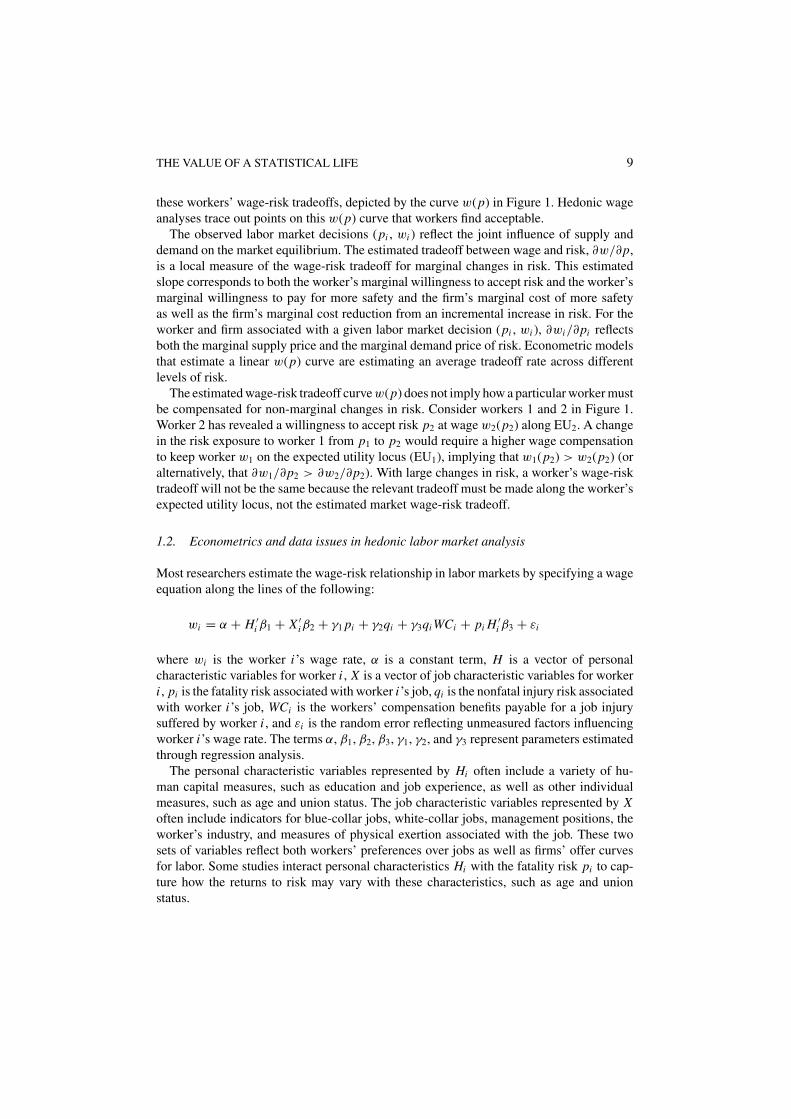
The firm’s demand for labor decreases with the total cost of employing a worker. Thecost of a worker may include the worker’s wage; training; benefits such as health insurance,vacation, child care; and the costs of providing a safe working environment. Because workercosts increase with the level of safety, for any given level of profits the firm must pay workersless as the safety level rises. Figure 1 depicts two firms with wage-risk offer curves (isoprofitcurves) with wage as an increasing function of risk, OC1 for firm 1 and OC2 for firm 2.For any given level of risk, workers prefer the wage-risk combination from the market offercurve with the highest wage level. The outer envelope of these offer curves is the marketopportunities locus w(p).
The worker’s supply of labor is in part a function of the worker’s preferences over wagesand risk. The labor supply is best characterized subject to several mild restrictions on prefer-ences. Consider a von Neumann-Morgenstern expected utility model with state-dependentutility functions.3 Let U (w) represent the utility of a healthy worker at wage w and let V (w)represent the utility of an injured worker at wage w. Typically, workers’ compensation afteran injury is a function of the worker’s wage. We assume that the relationship between work-ers’ compensation and the wage is subsumed into the functional form of V (w). Further,assume that workers prefer to be healthy than injured [U (w) > V (w)] and that the marginalutility of income is positive [U ′(w) > 0, V ′(w) > 0].4

8 VISCUSI AND ALDY
w1(p2)
w2(p2)
w1(p1)
p1 p2
Wage
Risk
EU1
w(p)
OC1
OC2
OC2
OC1
w(p)
EU2
EU1
EU2
Figure 1. Market process for determining compensating differentials.
Workers choose from potential wage-risk combinations along some market opportunitieslocus w(p) to maximize expected utility. In Figure 1, the tangency between the constantexpected utility locus EU1 and firm 1’s offer curve OC1 represents worker 1’s optimal jobrisk choice. Likewise, worker 2 maximizes expected utility at the tangency between EU2
and OC2. All wage-risk combinations associated with a given worker’s constant expectedutility locus must satisfy
Z = (1 − p)U (w) + pV (w).
The wage-risk tradeoff along this curve is given by
dw
dp= − Z p
Zw
= U (w) − V (w)
(1 − p)U ′(w) + pV ′(w)> 0,
so that the required wage rate is increasing in the risk level. The wage-risk tradeoff conse-quently equals the difference in the utility levels in the two states divided by the expectedmarginal utility of income.
Actual labor market decisions by workers can be depicted by the wage-risk combinationsat the tangencies of the offer curves and expected utility loci at points (p1, w1) and (p2, w2).All that is observable using market data are these points of tangency. Expanding beyondour two worker example, observations of a large set of workers can show the locus of
THE VALUE OF A STATISTICAL LIFE 9
these workers’ wage-risk tradeoffs, depicted by the curve w(p) in Figure 1. Hedonic wageanalyses trace out points on this w(p) curve that workers find acceptable.
The observed labor market decisions (pi , wi ) reflect the joint influence of supply anddemand on the market equilibrium. The estimated tradeoff between wage and risk, ∂w/∂p,is a local measure of the wage-risk tradeoff for marginal changes in risk. This estimatedslope corresponds to both the worker’s marginal willingness to accept risk and the worker’smarginal willingness to pay for more safety and the firm’s marginal cost of more safetyas well as the firm’s marginal cost reduction from an incremental increase in risk. For theworker and firm associated with a given labor market decision (pi , wi ), ∂wi/∂pi reflectsboth the marginal supply price and the marginal demand price of risk. Econometric modelsthat estimate a linear w(p) curve are estimating an average tradeoff rate across differentlevels of risk.
The estimated wage-risk tradeoff curve w(p) does not imply how a particular worker mustbe compensated for non-marginal changes in risk. Consider workers 1 and 2 in Figure 1.Worker 2 has revealed a willingness to accept risk p2 at wage w2(p2) along EU2. A changein the risk exposure to worker 1 from p1 to p2 would require a higher wage compensationto keep worker w1 on the expected utility locus (EU1), implying that w1(p2) > w2(p2) (oralternatively, that ∂w1/∂p2 > ∂w2/∂p2). With large changes in risk, a worker’s wage-risktradeoff will not be the same because the relevant tradeoff must be made along the worker’sexpected utility locus, not the estimated market wage-risk tradeoff.
1.2. Econometrics and data issues in hedonic labor market analysis
Most researchers estimate the wage-risk relationship in labor markets by specifying a wageequation along the lines of the following:
wi = α + H ′i β1 + X ′
iβ2 + γ1 pi + γ2qi + γ3qi WCi + pi H ′i β3 + εi
where wi is the worker i’s wage rate, α is a constant term, H is a vector of personalcharacteristic variables for worker i , X is a vector of job characteristic variables for workeri , pi is the fatality risk associated with worker i’s job, qi is the nonfatal injury risk associatedwith worker i’s job, WCi is the workers’ compensation benefits payable for a job injurysuffered by worker i , and εi is the random error reflecting unmeasured factors influencingworker i’s wage rate. The terms α, β1, β2, β3, γ1, γ2, and γ3 represent parameters estimatedthrough regression analysis.
The personal characteristic variables represented by Hi often include a variety of hu-man capital measures, such as education and job experience, as well as other individualmeasures, such as age and union status. The job characteristic variables represented by Xoften include indicators for blue-collar jobs, white-collar jobs, management positions, theworker’s industry, and measures of physical exertion associated with the job. These twosets of variables reflect both workers’ preferences over jobs as well as firms’ offer curvesfor labor. Some studies interact personal characteristics Hi with the fatality risk pi to cap-ture how the returns to risk may vary with these characteristics, such as age and unionstatus.

10 VISCUSI AND ALDY
1.2.1. Risk data. An ideal measure of on-the-job fatality and injury risk would reflectboth the worker’s perception of such risk and the firm’s perception of the risk. Because themarket opportunity locus reflects both workers’ preferences over income and risk and firms’preferences over costs and safety, information on both sets of beliefs would be necessaryto appropriately characterize the risk premium. However, very few studies have compiledworkers’ subjective preferences regarding risks (Viscusi, 1979; Viscusi and O’Connor, 1984;Gerking, de Haan, and Schulze, 1988; Liu and Hammitt, 1999) and there is no availableresearch on firms’ risk perceptions. If individuals’ and firms’ subjective risk perceptionsclosely reflect objective measures of fatality risk, then such objective risk data could be usedinstead as a proxy for unobserved subjective risk data.5 The standard approach in the litera-ture is to use industry-specific or occupation-specific risk measures reflecting an average ofat least several years of observations for fatalities, which tend to be relatively rare events.6
Measures of job-related fatality and injury risk have included self-reported risks basedon worker surveys and objective risk measures derived from actuarial tables, workers’compensation records, and surveys and censuses of death certificates. The choice of themeasure of fatality risk can significantly influence the magnitude of the risk premiumestimated through regression analysis. The nature of the risk measures also raise questionsabout possible errors in estimation and the need to correct the econometric specification toaddress them.
Several early papers on compensating differentials used the University of Michigan Sur-vey of Working Conditions and Quality of Employment Survey data that include severalqualitative measures of on-the-job risk. These measures utilize direct surveys of workersand their perceptions of their work environment. For example, Hamermesh (1978), Viscusi(1979, 1980), and Fairris (1989) estimated the hedonic wage equation with a dichoto-mous measure of injury risk based on a worker’s perception of whether his or her job is“dangerous.”7 The survey asked workers if their job exposed them to physical dangers orunhealthy conditions. These studies estimated statistically significant coefficients on this“risk” variable in some of the specifications. Duncan and Holmlund (1983) undertook asimilar analysis of compensating differentials with a “danger” variable in a study of maleworkers in Sweden.
Several papers on the U.S. labor market from the 1970s and early 1980s used actuarial data(Thaler and Rosen, 1975; Brown, 1980; Leigh, 1981; Arnould and Nichols, 1983). Thesestudies all employed a job-related risk measure based on data collected by the Societyof Actuaries for 1967. The Society of Actuaries data set provides fatality risk data for37 occupations. Across these 37 occupations, the annual risk averaged approximately 1in 1,000. This fatality risk exceeds averages from other data sets by nearly an order ofmagnitude. To the extent that these data reflect workers in extremely high risk jobs, theestimated wage-risk tradeoffs will suffer from a selection bias. As a result, one wouldexpect these estimates to be lower than found in more broadly representative samples,which has in fact proven to be the case.
Another difficulty is that the Society of Actuaries data do not distinguish fatalities causedby the job but rather reflect the overall fatality rates of people within a particular job category.For example, one of the highest risk occupations based on these actuarial ratings is actors,who typically face few risks other than unfavorable reviews.

THE VALUE OF A STATISTICAL LIFE 11
Several studies of U.S. and Canadian labor markets have used workers’ compensationrecords to construct risk measures (Butler, 1983; Dillingham, 1985; Leigh, 1991; Martinelloand Meng, 1992; Meng, 1991; Cousineau, Lacroix, and Girard, 1992; Lanoie, Pedro, andLaTour, 1995). Only three studies have used workers’ compensation data to evaluate com-pensating differentials in U.S. labor markets, which may reflect the decentralized natureand differences in information collection associated with state (not Federal) managementof U.S. workers’ compensation programs.8 In contrast, researchers in Canada can obtainworkers’ compensation-based risk data from Labour Canada (the labor ministry for theFederal government) and the Quebec government.
For analyses of the United States, the majority of the mortality risk studies have useddata collected by the U.S. Department of Labor Bureau of Labor Statistics (BLS). About 80percent of the U.S. nonfatal injury risk studies summarized below used BLS injury risk data.The BLS has compiled industry-specific fatality and injury risk data since the late 1960s.Through the early 1990s, BLS collected its data via a survey of industries, and reportedthe data at a fairly aggregated level, such as at the 2-digit and 3-digit Standard IndustrialClassification (SIC) code level. The aggregation and sampling strategy have elicited someconcerns about measurement error in the construction of the mortality risk variable (seeMoore and Viscusi, 1988a).
Concerns about the BLS fatality risk data led the National Institute of OccupationalSafety and Health (NIOSH) to collect information on fatal occupational injuries throughits National Traumatic Occupational Fatalities surveillance system (NTOF) since 1980.NIOSH compiles these data from death certificates managed by U.S. vital statistics report-ing units (NIOSH, 2000). These data are reported at the 1-digit SIC code level by state.Because NIOSH compiles data from a census of death certificates, it circumvents some ofthe concerns about sampling in the pre-1990s BLS approach. Some have raised concerns,however, about the accuracy of the reported cause of death in death certificates (Dormanand Hagstrom, 1998).
Comparing the BLS and NIOSH fatality risk data over time provides some interestingcontrasts. The original NIOSH data set for the fatality census averaged over 1980–1985has a mean fatality risk nearly 50 percent higher than a roughly comparable BLS dataset averaged over 1972–1982.9 Moreover, the BLS data had greater variation (a standarddeviation 95 percent greater than its mean) than the NTOF data, although the NIOSH dataalso had substantial variation (standard deviation 23 percent greater than its mean) (Mooreand Viscusi, 1988a).
Since 1992, the BLS has collected fatal occupational injury data through the Census ofFatal Occupational Injuries (CFOI). The BLS compiles information about each workplacefatality including worker characteristics and occupation, circumstances of the event, andpossible equipment involved. The BLS draws on multiple sources such as death certificates,workers’ compensation records, and other Federal and state agency reports. The BLS reportsthese fatality data by industry at the 4-digit SIC level. In contrast to the earlier comparisonsof BLS and NIOSH data, more recent years’ data on fatality risk collected through theCFOI now show that the BLS measure includes approximately 1,000 more fatalities peryear than the NIOSH measure (NIOSH, 2000). Table 1 illustrates the recent national ratesof job-related fatalities at the one-digit industry level for the four-year period in which both

12 VISCUSI AND ALDY
Table 1. U.S. Occupational fatality rates by industry, 1992–1995 nationalaverages.
Fatality rate per 100,000 workers
Industry NIOSH (NTOF) BLS (CFOI)
Agriculture, Forestry, & Fisheries 17.0 23.9
Mining 24.5 26.3
Construction 12.8 13.4
Manufacturing 3.6 3.8
Transportation & Utilities 10.4 10.6
Wholesale Trade 3.5 5.4
Retail Trade 2.8 3.6
Finance, Insurance, & Real Estate 1.1 1.5
Services 1.5 1.8
Sources: Rates constructed by authors based on Marsh and Layne (2001) andBLS (n.d.).
NIOSH and CFOI data are publicly available. In every instance the BLS measure shows ahigher risk mortality rate, which in some cases, such as wholesale trade, is quite substantial.
The risk variables used in several of the non-U.S. studies were based on job-relatedaccident and mortality data collected by foreign governments. For example, the data setsused in Shanmugam (1996/7, 1997, 2000, 2001) were from the Office of the Chief Inspectorof Factories in Madras. Several of the United Kingdom studies employ data provided by theOffice of Population Censuses and Surveys (Marin and Psacharopoulos, 1982; Sandy andElliott, 1996; Arabsheibani and Marin, 2000) while others used unpublished data from theU.K. Health and Safety Executive (Siebert and Wei, 1994). In their study of the South Koreanlabor market, Kim and Fishback (1999) obtained their accident data from the Ministry ofLabor. Few of these studies indicate whether the mortality risk data were derived fromsamples or censuses of job-related deaths.
While the large number of studies of labor markets around the world evaluated the com-pensating differential for an on-the-job death and/or on-the-job injury, very few attemptedto account for the risk of occupational disease. Lott and Manning (2000) used an alterna-tive data set to estimate the risk premium for jobs with higher cancer risk associated withoccupational exposure to various chemicals (see Section 2).
1.2.2. Wages and related data. Labor market studies of the value of risks to life andhealth match these risk measures to data sets on characteristics of wages, workers, andemployment. Some researchers survey workers directly to collect this information, such asGegax, Gerking, and Schulze (1991) for the United States, Lanoie, Pedro, and LaTour (1995)for Canada, Shanmugam (1996/7) for India, and Liu and Hammitt (1999) for Taiwan, amongothers. For the United States, researchers have also used the University of Michigan’s Surveyof Working Conditions (SWC), the Quality of Employment Survey (QES), the Bureau ofLabor Statistics’ Current Population Survey (CPS), the Panel Study of Income Dynamics

THE VALUE OF A STATISTICAL LIFE 13
(PSID), and decennial census data. Similar types of surveys undertaken in other countrieshave also provided the data necessary to undertake hedonic labor market analysis, suchas the General Household Survey in the United Kingdom (e.g., Siebert and Wei, 1994;Arabsheibani and Marin, 2000).
The dependent variable in virtually all labor market analyses has been a measure of thehourly wage. With some data sets, researchers have had to construct the wage measure fromweekly or annual labor earnings data. For some data sets, a worker’s after-tax wage rate isprovided, which can put wage and workers’ compensation benefits in comparable terms.While many studies have included pre-tax wages as the dependent variable, this would notlikely bias the results significantly so long as workers’ income levels and tax rates do notdiffer substantially. If the regression model includes workers’ compensation benefits, thenboth the wage and these benefits should be expressed in comparable terms (both in after-taxor both in pre-tax terms) to ensure proper evaluation of the benefits’ impacts on wages.10
Typically, researchers match a given year’s survey data on wages and worker and employ-ment characteristics with risk data for that year, or preferably, the average over a recent setof years. Some researchers have restricted their samples to subsets of the surveyed workingpopulation. For example, it is common to limit the analysis to full-time workers, and manyhave focused only on male, blue-collar workers. Restricting the sample in this manner par-tially addresses the measurement problem with industry-level risk values common to mostrisk data sets by including only those workers for whom the risk data are most pertinent.
1.2.3. Wage vs. log(wage). Most researchers have estimated the wage equation using linearand semi-logarithmic specifications. Choosing a preferred functional form from these twospecifications cannot be determined on theoretical grounds (see Rosen, 1974). To identifythe specification with greatest explanatory power, Moore and Viscusi (1988a) employed aflexible functional form given by the Box-Cox transformation. The Box-Cox transformationmodifies the dependent variable such that the estimated regression model takes the form:
wλi − 1
λ= α + H ′
i β1 + X ′iβ2 + γ1 pi + γ2qi + γ3qi WCi + pi H ′
i β3 + εi .
This approach presumes that a λ exists such that this model is normally distributed,homoskedastic, and linear in the regressors. Note that the case where λ → 0 represents thesemi-logarithmic functional form and the case where λ → 1 represents the linear functionalform. The flexible form under the Box-Cox transformation can test the appropriateness ofthese two restrictions on the form of the model. Using maximum likelihood methods, Mooreand Viscusi’s estimate for λ equaled approximately 0.3 for their data. While this value ismore consistent with a semi-logarithmic form than a linear form, the authors reject bothspecifications based on a likelihood ratio test. The estimated value of a statistical life basedon the Box-Cox transformed regression model, however, differed only slightly from thelog(wage) specification. Shanmugam (1996/7) replicated this flexible form evaluation withhis evaluation of compensating differentials in India. His maximum likelihood estimate forλ equaled approximately 0.2. While Shanmugam rejected the semi-logarithmic and linearmodels, he found that the semi-logarithmic functional form also generated results closer tothose found with the unrestricted flexible form.11
14 VISCUSI AND ALDY
1.2.4. Errors in variables problem with risk measures. Every compensating differentialstudy employs a less than perfect measure of any particular worker’s job-related fatalityrisk. The majority of these studies have used fatality risk measures from the BLS averagedacross entire industries. Such an approach, however, suffers from measurement error. Asnoted above, some researchers have found that the pre-1992 BLS data sets (and NIOSH datasets to a lesser extent) suffer from incomplete reporting. The industry averages constructedby the BLS do not exactly reflect realized industry averages. Further, applying industryaverages to individuals may result in errors associated with matching workers to industriesdue to response error in worker surveys. Mellow and Sider (1983) evaluated several surveysthat asked workers and their employers to identify the workers’ industry and occupation(among other questions). In their assessment of the January 1977 Current Population Survey,84 percent of workers and their employers agreed on industry affiliation at the three-digitSIC code level while only 58 percent agreed on the three-digit occupational status. Merginga worker characteristics data set with a risk measure data set based on industry affiliation(or occupation status) can result in a mismatch of worker characteristics and industry risk.Mellow and Sider’s statistical analysis of the 16 percent “mismatched” workers by industryaffiliation showed that the errors in matching reduced the compensating differential forinjury risk by about 50 percent in their samples.
Even with a perfect industry measure of fatality risk and appropriate matching of workersand their industry, measurement error still exists since some workers bear risk that differsfrom their industry’s average. For example, different occupations within an industry maypose different levels of risk. This measurement error can be characterized as:
pi = p∗i
+ ηi ,
where pi reflects the observed industry average fatality risk, p∗i reflects the unobserved (to
the econometrician) fatality risk associated with worker i’s job, and ηi reflects the deviationof that job’s risk from the industry average. Random measurement error will result in adownward bias on coefficient estimates, and the least squares estimate of the coefficient onfatality risk in this example would be inconsistent:
γ̂1,OLSp→
(σ 2
p
σ 2p + σ 2
η
)γ1
where the signal-noise ratio determines the extent of the downward bias towards zero.In addition to the downward effect on the risk coefficient, applying industry-level risk
data to individual observations may also induce some correlation in the residuals amongindividuals within industries. Robust (White) standard errors would not appropriately cor-rect for this correlation and result in inappropriately small standard errors. Hersch (1998)and Viscusi and Hersch (2001) employ robust standard errors correcting for within-group(within-industry) correlation.
1.2.5. Omitted variables bias and endogeneity. Failing to capture all of the determinantsof a worker’s wage in a hedonic wage equation may result in biased results if the unobserved

THE VALUE OF A STATISTICAL LIFE 15
variables are correlated with observed variables. Dangerous jobs are often unpleasant inother respects. Omission of non-pecuniary characteristics of a job may bias the estimatedrisk premium if an omitted variable is correlated with risk. For example, one may find acorrelation between injury risk and physical exertion required for a job or risk and environ-mental factors such as noise, heat, or odor. While some studies have attempted to controlfor these unobservables by including industry or occupation dummy variables (see below),a model may still suffer from omitted variables bias.
Several studies have explored how omitting injury risk affects the estimation of mortalityrisk. Viscusi (1981) found that omitting injury risk resulted in a positive bias in the mortalityrisk measure for union affiliated workers. Cousineau, Lacroix, and Girard (1992) also foundthat omitting injury risk may cause a positive bias in the estimation of the coefficienton mortality risk. The high correlation (collinearity) between injury and mortality risks,however, can make joint estimation difficult. Some studies have attempted to estimateregression equations with both types of risk and have found non-significant coefficients onat least one of the measures, including Smith (1976), Leigh (1981), Dillingham and Smith(1984) and Kniesner and Leeth (1991).
While including injury risk in a regression model could address concern about one omit-ted variable, other possible influences on wages that could be correlated with mortalityrisk may not be easily measured. Several papers have investigated this bias. Garen (1988)notes that “individuals may systematically differ in unobserved characteristics which affecttheir productivity and earnings in dangerous jobs and so these unobservables will affecttheir choice of job risk” (p. 9). One example Garen offers is “coolheadedness,” whichmay make a worker more productive under the stresses of a dangerous job but may notbe relevant in a safe job. In this case, an econometrician would prefer to include boththe mortality risk variable and the interaction or the mortality risk variable with a vari-able measuring coolheadedness as regressors in the hedonic labor market model. Failingto include this interaction term results in biased least squares estimation. Garen attemptsto address this concern with an instrumental variables technique, although subsequent re-searchers such as Hwang, Reed, and Hubbard (1992) have noted the difficulty in identifyingappropriate instruments for his procedure. Employing this instrumental variables technique,Garen found a mortality risk premium about double what the standard least squares modelproduced.
The significant increase in the risk premium associated with a method to account forunobserved productivity is consistent with the theoretical and simulation findings in Hwang,Reed, and Hubbard (1992). They estimate that for plausible parameter estimates, modelsthat fail to account for heterogeneity in unobserved productivity may bias estimates of therisk premium by about 50 percent and could result in incorrectly (negative) signing of therisk variable. With the exception of some non-union samples in several studies (e.g., Dorsey,1983; Dickens, 1984), the empirical literature presents very little evidence of this wrongsigning. Siebert and Wei (1994) have also found that accounting for the endogeneity ofrisk can increase the risk premium compared to a standard least squares approach. Recenttheoretical research, however, has also illustrated the potential for over-estimating the riskpremium by failing to control for unobservables (Shogren and Stamland, 2002). They notethat workers with the ability to avoid injury select into risky jobs while those less able to avoid
16 VISCUSI AND ALDY
injury (“clumsy” workers) select into less-risky jobs. They argue that risk premiums couldbe overestimated by a factor of four with plausible parameter estimates in their simulations.Whether there will be such biases hinges on the monitorability of an individual’s safety-related productivity. If these differences are monitorable, as in Viscusi and Hersch (2001),there will be a separating compensating differential equilibrium for workers of differentriskiness.
Viscusi and Hersch (2001) note that differences in workers’ preferences over risk canaffect the shape of their indifference curves and workers’ safety behavior and, by affectingfirms’ cost to supply safety, can influence firms’ offer curves. They evaluated the wage-risk(injury) tradeoff of workers with a data set that includes measures of risk preferences (e.g.,smoking status) and measures of workers’ prior accident history. While smokers work, onaverage, in industries with higher injury risk than non-smokers, smokers also are morelikely to have a work-related injury controlling for industry risk. Smokers also are moreprone to have had a recent non-work-related accident. As a result, Viscusi and Hersch findthat nonsmokers receive a greater risk premium in their wages than do smokers becausethe safety effect flattens smokers’ offer curves enough to offset smokers’ preferences forgreater wages at higher risk levels.
To address potential omitted variable bias arising from differences in worker characteris-tics, employing a panel data set could allow one to difference out or dummy out individual-specific unobservables, so long as these are constant throughout the time period covered bythe panel. Unfortunately, very few data sets exist that follow a set of workers over a periodof several years. Brown (1980) used the National Longitudinal Study Young Men’s sampleover 1966–1973 (excluding 1972) with the Society of Actuaries mortality risk data. Whilehe reported results that were not consistent with the theory of compensating differentials fora variety of nonpecuniary aspects of employment, he did estimate a positive and statisticallysignificant coefficient on the mortality risk variable. Brown noted that his estimate of therisk premium was nearly three times the size of the estimate in Thaler and Rosen (1975),which first used the Society of Actuaries mortality risk data.
1.2.6. Compensating differentials for risk or inter-industry wage differentials. Severalrecent papers have claimed that estimates of risk premiums in this kind of wage regressionanalysis actually reflect industry wage premiums because the fatality risk variables typicallyreflect industry-level risk (Leigh, 1995; Dorman and Hagstrom, 1998). Both Leigh andDorman and Hagstrom evaluate the proposition that risk premiums simply reflect industrypremiums by comparing compensating differential models without dummy variables forindustry affiliation of each worker with models that include such dummy variables.
Their claim that industry premiums mask as risk premiums in these wage regressionssuffers from several deficiencies. First, a large number of studies have included industrydummy variables in their statistical analyses and found significant compensating differen-tials for risk. For example, the first wage-risk tradeoff study by Smith (1974) employed sixindustry dummies and yielded a statistically significant compensating differential for risk.Viscusi (1978a) included 25 industry dummy variables in his analysis based on the Surveyof Working Conditions danger variable (0, 1 variable reflecting a worker’s subjective per-ception of on-the-job risk), although he excluded the dummy variables from the analysis
THE VALUE OF A STATISTICAL LIFE 17
based on the industry-level BLS risk data.12 In both sets of analyses, danger and the BLSrisk measure were statistically significant and generated very similar estimates of the riskpremium. Freeman and Medoff (1981) found a statistically significant risk premium in theiranalyses that included 20 industry dummy variables and the BLS injury rate measure. Intheir evaluation of the U.K. labor market with an occupational mortality risk variable, Marinand Psacharopoulos (1982) found a statistically significant risk coefficient while their SICcode dummies were insignificant. Dickens (1984) estimated regression models with theBLS fatality risk measure and 20 industry dummy variables (1- and 2-digit SIC code in-dustries). For the union sample, he found a positive and statistically significant coefficienton risk. Leigh and Folsum (1984) included 2-digit SIC code industry dummy variablesin their wage regressions, and they found statistically significant coefficients on mortalityrisk in all eight mortality risk models reported. Dillingham (1985) estimated regressionmodels with industry dummy variables (at the 1-digit SIC code level) and without. In bothcases, he found statistically significant and positive coefficients on his measure of mortalityrisk. Moreover, the coefficients were virtually identical (0.0023 vs. 0.0022), although thestandard error was higher for the model with industry dummy variables (perhaps related torisk-industry dummy variable collinearity). Cousineau, Lacroix, and Girard (1992) included29 industry variables in their evaluation of the Canadian labor market that estimated statis-tically significant coefficients on both injury and mortality risks. Lott and Manning (2000)included 13 industry dummy variables in their evaluation of long-term cancer risks in U.S.labor markets, and found a statistically significant risk premium based on industry-levelmeasures of carcinogen exposure.
Second, inserting industry dummy variables into the regression equation induces multi-collinearity with the risk variable. Previous researchers such as Viscusi (1979) have notedthis as well. Hamermesh and Wolfe (1990) employed dummy variables for five major indus-tries in their analysis of injury risk on wages. They note that a finer breakdown by industrycould be used. A complete set of dummy variables at the 3-digit SIC code level, however,would completely eliminate all variation in the injury risk variable, which is measured atthe 3-digit SIC code level (p. S183). While multicollinearity does not affect the consistencyof the parameter estimates, it will increase standard errors.
This induced multicollinearity is also evident in the Dorman and Hagstrom results forthe models using NIOSH fatality risk data.13 Dorman and Hagstrom interact the NIOSHfatality risk measure by a dummy variable for union status (and for non-union status inthe second set of regressions). Contrary to their hypothesis, including industry dummyvariables does not reduce the coefficient in the union-risk interaction models. Inducingmulticollinearity does depress the t-statistics slightly, although not enough to render thecoefficients statistically insignificant. The models with the non-union-risk interaction reflectthe induced multicollinearity, as the t-statistics fall below levels typically associated withstatistical significance moving from the standard model to the industry dummy model. Whilethe coefficients in these industry dummy-augmented models fall from their levels in thestandard models, they are not statistically different from the standard models’ coefficients.Based on the NIOSH fatality risk data, the Dorman and Hagstrom results appear to illustratethat including collinear regressors (industry variables) can increase standard errors but notsignificantly affect the magnitudes of the parameter estimates.
18 VISCUSI AND ALDY
2. The value of a statistical life based on U.S. labor market studies
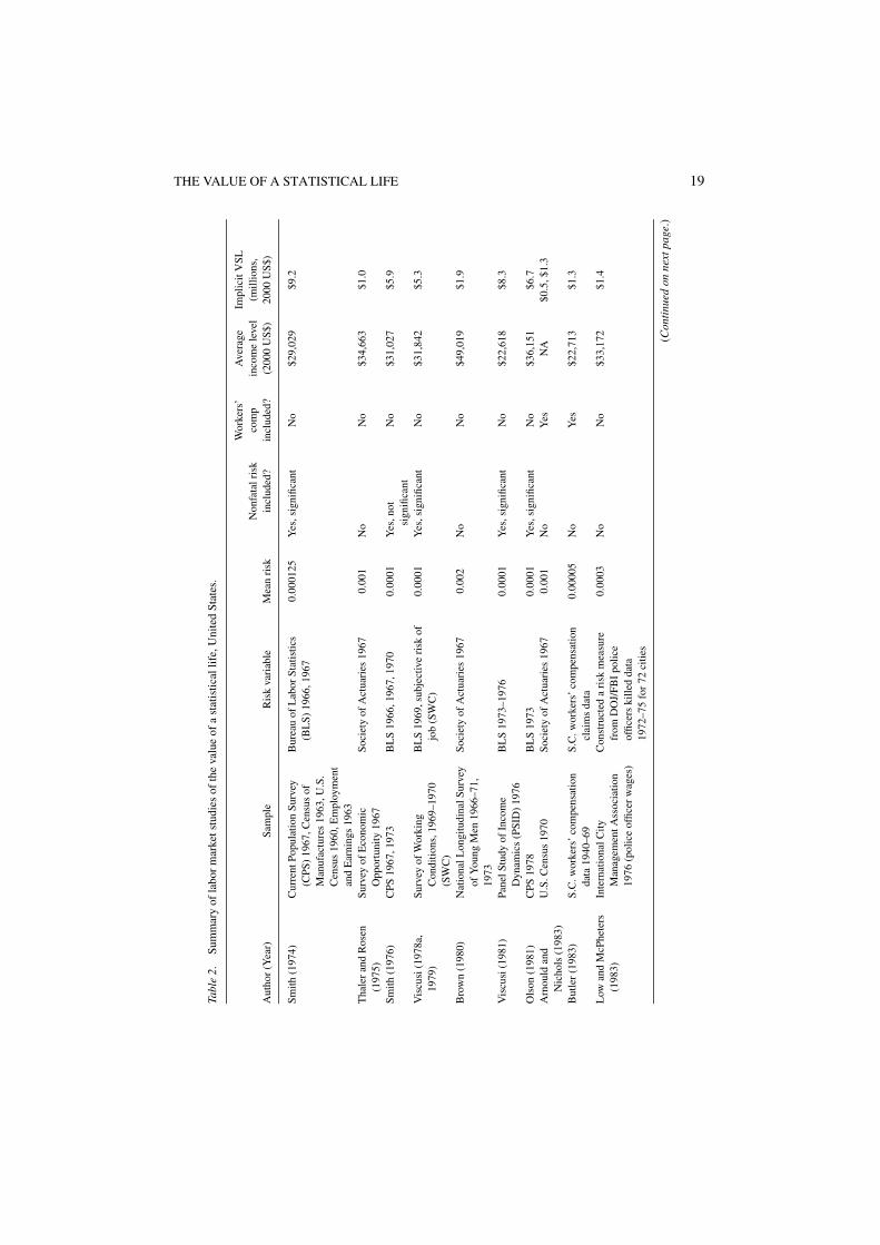
The value of a statistical life should not be considered a universal constant or some “rightnumber” that researchers aim to infer from market evidence. Rather, the VSL reflects thewage-risk tradeoffs that reflect the preferences of workers in a given sample. Moreover,transferring the estimates of a value of a statistical life to non-labor market contexts, asis the case in benefit-cost analyses of environmental health policies for example, shouldrecognize that different populations have different preferences over risks and different valueson life-saving. If people face continuous safety choices in a variety of contexts, however,the same individual should exhibit the same risk-money tradeoff across different contexts,provided the character of the risks is the same. Researchers have undertaken more than30 studies of compensating differentials for risk in the U.S. labor market. Some studieshave evaluated the wage-risk tradeoff for the entire labor force, while others have focusedon subsamples such as specific occupations (e.g., police officers in Low and McPheters,1983), specific states (e.g., South Carolina in Butler, 1983), blue-collar workers only (e.g.,Dorman and Hagstrom, 1998; Fairris, 1989), males only (e.g., Berger and Gabriel, 1991),and union members only (e.g., Dillingham and Smith, 1984). These hedonic labor marketstudies also vary in terms of their choice of mortality risk variable, which can significantlyinfluence the estimation of a value of a statistical life (for comparison of NIOSH and BLSdata, refer to Moore and Viscusi, 1988a; Dorman and Hagstrom, 1998).
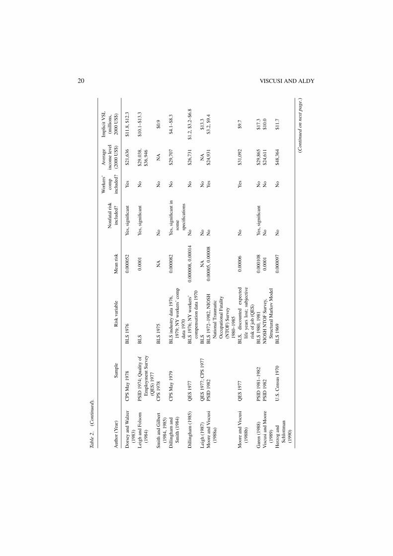
Table 2 summarizes the estimated VSLs for the U.S. labor market from the literatureover the past three decades.14 Because some studies provided multiple estimates, in theseinstances we provide illustrative results based on the principal specification in the analysis.Table 2 provides a sense of the magnitude and range of U.S. labor market VSLs andillustrates the influence of factors such as income and the magnitude of risk exposure as wellas specification issues such as including nonfatal injury risk and worker’s compensation.15
Viscusi (1993) reported that most surveyed studies fall within a $3.8–$9.0 million range,when converted into year 2000 dollars.16,17 While we include more papers from the UnitedStates as well as findings from other countries, the general conclusion remains unchanged.Half of the studies of the U.S. labor market reveal a value of a statistical life range from $5million to $12 million. Estimates below the $5 million value tend to come from studies thatused the Society of Actuaries data, which tends to reflect workers who have self-selectedthemselves into jobs that are an order of magnitude riskier than the average. Many of thestudies yielding estimates beyond $12 million used structural methods that did not estimatethe wage-risk tradeoff directly or were derived from studies in which the authors reportedunstable estimates of the value of a statistical life. Our median estimated VSL from Table 2is about $7 million, which is in line with the estimates from the studies that we regard asmost reliable. In terms of methodology, we are more confident in the results presented inViscusi (1978a, 1979), which include the most extensive set of non-pecuniary characteristicsvariables to explain workers’ wages, and the results presented in Moore and Viscusi (1988a),which include the NIOSH mortality risk data in lieu of the pre-1992 BLS mortality riskdata.
A salient research issue of policy importance is the effect of income levels on the wage-risk tradeoff. For example, Hamermesh (1999) notes that as wage inequality has increased
THE VALUE OF A STATISTICAL LIFE 19
Tabl
e2.
Sum
mar
yof
labo
rm
arke
tstu
dies
ofth
eva
lue
ofa
stat
istic
allif
e,U
nite
dSt
ates
.
Wor
kers
’A
vera
geIm
plic
itV
SLN
onfa
talr
isk
com
pin
com
ele
vel
(mill
ions
,A
utho
r(Y
ear)
Sam
ple
Ris
kva
riab
leM
ean
risk
incl
uded
?in
clud
ed?
(200
0U
S$)
2000
US$
)
Smith
(197
4)C
urre
ntPo
pula
tion
Surv
ey(C
PS)
1967
,Cen
sus
ofM
anuf
actu
res
1963
,U.S
.C
ensu
s19
60,E
mpl
oym
ent
and
Ear
ning
s19
63
Bur
eau
ofL
abor
Stat
istic
s(B
LS)
1966
,196
70.
0001
25Y
es,s
igni
fican
tN
o$2
9,02
9$9
.2
Tha
ler
and
Ros
en(1
975)
Surv
eyof
Eco
nom
icO
ppor
tuni
ty19
67So
ciet
yof
Act
uari
es19
670.
001
No
No
$34,
663
$1.0
Smith
(197
6)C
PS19
67,1
973
BL
S19
66,1
967,
1970
0.00
01Y
es,n
otsi
gnifi
cant
No
$31,
027
$5.9
Vis
cusi
(197
8a,
1979
)Su
rvey
ofW
orki
ngC
ondi
tions
,196
9–19
70(S
WC
)
BL
S19
69,s
ubje
ctiv
eri
skof
job
(SW
C)
0.00
01Y
es,s
igni
fican
tN
o$3
1,84
2$5
.3
Bro
wn
(198
0)N
atio
nalL
ongi
tudi
nalS
urve
yof
You
ngM
en19
66–7
1,19
73
Soci
ety
ofA
ctua
ries
1967
0.00
2N
oN
o$4
9,01
9$1
.9
Vis
cusi
(198
1)Pa
nelS
tudy
ofIn
com
eD
ynam
ics
(PSI
D)
1976
BL
S19
73–1
976
0.00
01Y
es,s
igni
fican
tN
o$2
2,61
8$8
.3
Ols
on(1
981)
CPS
1978
BL
S19
730.
0001
Yes
,sig
nific
ant
No
$36,
151
$6.7
Arn
ould
and
Nic
hols
(198
3)U
.S.C
ensu
s19
70So
ciet
yof
Act
uari
es19
670.
001
No
Yes
NA
$0.5
,$1.
3
But
ler
(198
3)S.
C.w
orke
rs’
com
pens
atio
nda
ta19
40–6
9S.
C.w
orke
rs’
com
pens
atio
ncl
aim
sda
ta0.
0000
5N
oY
es$2
2,71
3$1
.3
Low
and
McP
hete
rs(1
983)
Inte
rnat
iona
lCity
Man
agem
entA
ssoc
iatio
n19
76(p
olic
eof
ficer
wag
es)
Con
stru
cted
ari
skm
easu
refr
omD
OJ/
FBI
polic
eof
ficer
ski
lled
data
1972
–75
for
72ci
ties
0.00
03N
oN
o$3
3,17
2$1
.4
(Con
tinu
edon
next
page
.)
20 VISCUSI AND ALDY
Tabl
e2.
(Con
tinu
ed).
Wor
kers
’A
vera
geIm
plic
itV
SLN
onfa
talr
isk
com
pin
com
ele
vel
(mill
ions
,A
utho
r(Y
ear)
Sam
ple
Ris
kva
riab
leM
ean
risk
incl
uded
?in
clud
ed?
(200
0U
S$)
2000
US$
)
Dor
sey
and
Wal
zer
(198
3)C
PSM
ay19
78B
LS
1976
0.00
0052
Yes
,sig
nific
ant
Yes
$21,
636
$11.
8,$1
2.3
Lei
ghan
dFo
lsom
(198
4)PS
ID19
74;Q
ualit
yof
Em
ploy
men
tSur
vey
(QE
S)19
77
BL
S0.
0001
Yes
,sig
nific
ant
No
$29,
038,
$36,
946
$10.
1–$1
3.3
Smith
and
Gilb
ert
(198
4,19
85)
CPS
1978
BL
S19
75N
AN
oN
oN
A$0
.9
Dill
ingh
aman
dSm
ith(1
984)
CPS
May
1979
BL
Sin
dust
ryda
ta19
76,
1979
;NY
wor
kers
’co
mp
data
1970
0.00
0082
Yes
,sig
nific
anti
nso
me
spec
ifica
tions
No
$29,
707
$4.1
–$8.
3
Dill
ingh
am(1
985)
QE
S19
77B
LS
1976
;NY
wor
kers
’co
mpe
nsat
ion
data
1970
0.00
0008
,0.0
0014
No
No
$26,
731
$1.2
,$3.
2–$6
.8
Lei
gh(1
987)
QE
S19
77;C
PS19
77B
LS
NA
No
No
NA
$13.
3M
oore
and
Vis
cusi
(198
8a)
PSID
1982
BL
S19
72–1
982,
NIO
SHN
atio
nalT
raum
atic
Occ
upat
iona
lFat
ality
(NT
OF)
Surv
ey19
80–1
985
0.00
005,
0.00
008
No
Yes
$24,
931
$3.2
,$9.
4
Moo
rean
dV
iscu
si(1
988b
)Q
ES
1977
BL
S,di
scou
nted
expe
cted
life
year
slo
st;
subj
ectiv
eri
skof
job
(QE
S)
0.00
006
No
Yes
$31,
092
$9.7
Gar
en(1
988)
PSID
1981
–198
2B
LS
1980
,198
10.
0001
08Y
es,s
igni
fican
tN
o$2
9,86
5$1
7.3
Vis
cusi
and
Moo
re(1
989)
PSID
1982
NIO
SHN
TO
FSu
rvey
,St
ruct
ural
Mar
kov
Mod
el0.
0001
No
No
$24,
611
$10.
0
Her
zog
and
Schl
ottm
an(1
990)
U.S
.Cen
sus
1970
BL
S19
690.
0000
97N
oN
o$4
8,36
4$1
1.7
(Con
tinu
edon
next
page
.)

THE VALUE OF A STATISTICAL LIFE 21Ta
ble
2.(C
onti
nued
).
Wor
kers
’A
vera
geIm
plic
itV
SLN
onfa
talr
isk
com
pin
com
ele
vel
(mill
ions
,A
utho
r(Y
ear)
Sam
ple
Ris
kva
riab
leM
ean
risk
incl
uded
?in
clud
ed?
(200
0U
S$)
2000
US$
)
Moo
rean
dV
iscu
si(1
990b
)PS
ID19
82N
IOSH
NT
OF
Surv
ey,
Stru
ctur
alL
ife
Cyc
leM
odel
0.00
01N
oN
o$2
4,61
1$2
0.8
Moo
rean
dV
iscu
si(1
990c
)PS
ID19
82N
IOSH
NT
OF
Surv
ey,
Stru
ctur
alIn
tegr
ated
Lif
eC
ycle
Mod
el
0.00
01Y
esY
es$2
4,61
1$2
0.8
Kni
esne
ran
dL
eeth
(199
1)C
PS19
78N
IOSH
NT
OF
surv
ey19
80–1
985
0.00
04Y
es,s
igni
fican
tin
som
esp
ecifi
catio
ns
Yes
$33,
627
$0.7
Geg
ax,G
erki
ng,a
ndSc
hulz
e(1
991)
Aut
hors
’m
ails
urve
y19
84W
orke
rs’
asse
ssed
fata
lity
risk
atw
ork
1984
0.00
09N
oN
o$4
1,39
1$2
.1
Lei
gh(1
991)
QE
S19
72–3
,QE
S19
77,
PSID
1974
,198
1,L
ongi
tudi
nalQ
ES
1973
–197
7,C
PSJa
nuar
y19
77
BL
S19
79,w
orke
rs’
com
pens
atio
nda
tafr
om11
stat
es19
77–1
980
0.00
0134
No
No
$32,
961
$7.1
–$15
.3
Ber
ger
and
Gab
riel
(199
1)U
SC
ensu
s19
80B
LS
1979
0.00
008–
0.00
0097
No
No
$46,
865,
$48,
029
$8.6
,$10
.9
Lei
gh(1
995)
PSID
1981
,CPS
Janu
ary
1977
,QE
S19
77B
LS
1976
,79–
81an
dN
IOSH
1980
–85
0.00
011–
0.00
013
No
No
$29,
587
$8.1
–$16
.8
Dor
man
and
Hag
stro
m(1
998)
PSID
1982
BL
S19
79–1
981,
1983
,19
85,1
986;
NIO
SHN
TO
F19
80–1
988
0.00
0123
–0.0
0016
39Y
esY
es$3
2,24
3$8
.7–$
20.3
Lot
tand
Man
ning
(200
0)C
PSM
arch
1971
and
Mar
ch19
85H
icke
y-K
earn
eyca
rcin
ogen
icex
posu
re19
72–1
974,
NIO
SHN
atio
nalO
ccup
atio
nal
Exp
osur
eSu
rvey
1981
–198
3
NA
No
No
$30,
245
$1.5
,$3.
0($
2.0,
$4.0
)†
† Lot
tand
Man
ning
(200
0)es
timat
ere
pres
ents
the
valu
eof
avoi
ding
ast
atis
tical
fata
lcan
cer
case
with
anas
sum
edla
tenc
ype
riod
of10
year
s(d
isco
unte
dat
3pe
rcen
t).
The
repo
rted
valu
esfr
omth
eir
pape
rw
ithou
tdis
coun
ting
ofth
isla
tenc
ype
riod
are
pres
ente
din
pare
nthe
ses.
22 VISCUSI AND ALDY
over the last several decades, so have on-the-job mortality risks diverged. He notes thatworkplace safety is highly income-elastic. This result is related to the findings in Viscusi(1978b) that the value of a statistical life is increasing in worker wealth. Similarly, Viscusiand Evans (1990) have estimated the income elasticity of the value of statistical job injuryrisks to be 0.6 to 1.0. The effect of income on the wage-risk tradeoff is evident in a historicalevaluation of employment risks as well. Kim and Fishback (1993) estimated compensatingdifferentials for mortality risk in the railroad industry over the period 1893–1909 and foundimplicit values of statistical life on the order of $150,000 in today’s dollars.18 Our meta-analysis below examines the role of income differences in generating the variation in VSLestimates.
While most hedonic labor market studies focus on the risk of accidental death or accidentalinjury, several papers have attempted to explore the effect of occupational disease. Lott andManning (2000) evaluated the effect of carcinogen exposure on workers’ wages within thecontext of changing employer liability laws. In lieu of the standard mortality risk measures,the authors employ the Hickey and Kearney carcinogen index, which represents workercarcinogen exposure at the 2-digit SIC code level.19 They find that workers’ wages reflect arisk premium for carcinogen exposure. Lott and Manning convert their results into a valueof a statistical life assuming that the index is a proportional representation of the actualprobability of getting occupational-related cancer, that 10–20 percent of all cancer deathsresult from occupational exposures, and that the probability of a worker getting cancerranges from 0.04 to 0.08 percent per year. We have modified their reported VSL range toaccount for a latency period.20 Based on these assumptions, the authors estimate that thevalue of a statistical life based on occupational cancer would range from $1.5–$3.0 million.Assuming that occupational cancers, however, comprise a smaller fraction of all cancerdeaths would increase the implicit VSL.21
Several early papers in the literature did not find statistically significant compensating dif-ferentials for on-the-job mortality risk. For example, Leigh (1981) estimated a risk premiumfor injuries but not for fatalities. Dorsey (1983) likewise did not find a mortality-based riskpremium. The Leigh study coupled the Society of Actuaries mortality data with BLS injurydata. The combination of greater measurement error in the data and the high correlation be-tween injury risks and mortality risks probably led to the insignificance of the mortality riskvariable. The Dorsey study uses industry-level averages, instead of worker-specific values,as its unit of observation. This averaging across industry for wages and related explanatoryvariables may have reduced the variation necessary to discern the effects of job-specificinfluences on wage, such as job risk.
More recent papers by Leigh (1995) and Dorman and Hagstrom (1998) also do not findcompensating differentials in many model specifications. As discussed above, we do not findtheir inter-industry wage differential discussion compelling. Nevertheless, Table 2 includestheir results based on the NIOSH data with industry dummy variables.22
Some of these analyses of U.S. labor markets investigated the potential heterogeneityin the risk preferences of workers in the labor force in which there is worker sorting bylevel of risk. The empirical issue is whether the wage-risk tradeoff takes a linear or concaveshape. A linear form would imply that an incremental increase of risk in the labor marketrequires a proportional increase in the wage differential. A concave form, however, would
THE VALUE OF A STATISTICAL LIFE 23
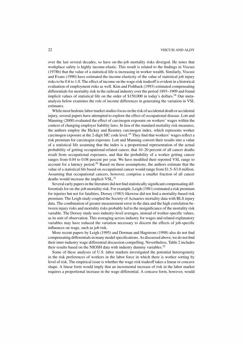
Figure 2. The value of a statistical life as a function of mortality risk.
imply a less than proportional increase in the wage differential, perhaps reflecting sortingby workers based on their risk preferences.
To evaluate the shape of this tradeoff, one can modify the wage equation regressionmodel to include both mortality risk and the square of mortality risk. If the latter term is notsignificant, then the wage-risk tradeoff is linear for the range of risks and wages coveredby the study’s sample. If the squared term is significant and negative, then the wage-risktradeoff takes a concave form. Viscusi (1981), Olson (1981), Dorsey and Walzer (1983), andLeigh and Folsum (1984) all found evidence that the risk-wage tradeoff curve is concave.23
All four studies include regression models with a quadratic representation of mortality risk.Figure 2 illustrates how the value of a statistical life varies with mortality risk for a sample
of six regression models from these four papers. Viscusi (1981; linear) and Leigh and Folsum(1984; linear) represent regression models where the dependent variable is the hourly wagewhile the other four lines represent regression models with the logarithm of the wage as thedependent variable. All six models include measures of nonfatal injury risks (probability ofa lost-workday accident and, in some cases, duration of lost-workday accident). The slopesof the risk-VSL lines in this figure are similar within the wage-specification type where thewage-based models appear to have a steeper tradeoff than do the logarithm of wage-basedmodels (with the exception of the Dorsey and Walzer model, although this may reflect thefact that the sample in their study faced mortality risks 2 to 3 times smaller on average thanthe samples in the other studies). Based on these models, populations of individuals whoselect into jobs with very minor risks (e.g., on the order of 1 in 100,000) have implicit valuesof statistical life ranging from $12 to $22 million. Increasing the risk ten-fold, to levels thatare close to the mean mortality risks in these studies, modestly reduces the VSL into therange of $10 to $18 million. Figure 2 illustrates that very high risks result in small valuesof statistical lives, although caution should be exercised when considering extrapolationsbeyond the samples’ ranges.
24 VISCUSI AND ALDY
3. Evidence of the value of a statistical life from U.S. housing and product markets
Housing and product market decisions also reflect individual tradeoffs between mortalityrisk and money. The main methodological difference is that economists typically estimatea hedonic price equation rather than a hedonic wage equation. The underlying theory isessentially the same, as comparison of Rosen (1974) with the wage equation analysis abovewill indicate.
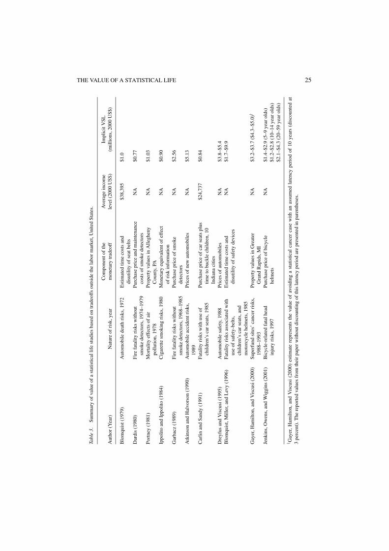
Table 3 presents the results from eleven studies that evaluated the price-risk tradeoffsfor seatbelt use, cigarette smoking, home fire detectors, automobile safety, bicycle helmets,and housing price responses to hazardous waste site risks.24 The studies in general find animplicit value of a statistical life on the same order of magnitude as the labor market studies,although they tend to be a little lower.
The lower estimates may reflect several characteristics of these studies that distinguishthem from the labor market studies. First, some product decisions do not provide a continuumof price-risk opportunities (unlike the labor market that does offer a fairly continuous array ofwage-risk employment options) but rather a discrete safety decision. For example, Dardis’(1980) evaluation of smoke detectors represents such a discrete choice. In such a case,the consumer’s decision to purchase a smoke detector reveals only the lower bound on thewillingness to pay for the reduced risk. Similarly, the study by Jenkins, Owens, and Wiggins(2001) examines the purchase of bicycle helmets. It is interesting, however, that their resultsshow VSLs increasing over the first half of the life cycle.
Second, the types of products considered in some studies may induce selection basedon risk preferences. For example, the low estimated VSL for cigarette smokers found byIppolito and Ippolito (1984) presumably reflects the non-random character of the smok-ing population. Their research focuses on cigarette smokers, and they estimate a VSLlower than from most product market studies. The lower VSL is consistent with the find-ings in Hersch and Viscusi (1990) and Viscusi and Hersch (2001) who find that indi-viduals who engage in risky behaviors, such as cigarette smoking and driving withoutseatbelts, have lower implicit values for injury than do those who do not engage in suchbehavior.
Third, several studies are based on inferred, instead of observed, price-risk tradeoffs.Consider the seat belt, child seat, and motorcycle helmet studies by Blomquist (1979),Carlin and Sandy (1991) and Blomquist, Miller, and Levy (1996). In these studies, drivers’,occupants’, or riders’ safety is traded off with the time to secure a seat belt or a child seat orto put on a helmet. The authors assume a given time cost—for example, Blomquist assumesthat it takes 8 seconds to secure a seat belt. Then this time is monetized at the individual’swage rate (or a fraction thereof in Blomquist, 1979, and Blomquist, Miller and Levy, 1996).Unlike labor market studies where the monetary value of the attribute in question (job wage)is observed, these studies do not observe the actual time drivers take to buckle their seatbelts. The amount of time is estimated separately. In addition to time costs, there are otheraspects of seat belt or helmet use, such as the costs of discomfort of wearing a seatbelt ora helmet, which would increase the implicit valuation of a statistical life derived by thismethodology. While some of these studies attempt to include estimates of these potentiallylarge costs, the estimates are imprecise.
THE VALUE OF A STATISTICAL LIFE 25
Tabl
e3.
Sum
mar
yof
valu
eof
ast
atis
tical
life
stud
ies
base
don
trad
eoff
sou
tsid
eth
ela
bor
mar
ket,
Uni
ted
Stat
es.
Com
pone
ntof
the
Ave
rage
inco
me
Impl
icit
VSL
Aut
hor
(Yea
r)N
atur
eof
risk
,yea
rm
onet
ary
trad
eoff
leve
l(20
00U
S$)
(mill
ions
,200
0U
S$)
Blo
mqu
ist(
1979
)A
utom
obile
deat
hri
sks,
1972
Est
imat
edtim
eco
sts
and
disu
tility
ofse
atbe
lts$3
8,39
5$1
.0
Dar
dis
(198
0)Fi
refa
talit
yri
sks
with
out
smok
ede
tect
ors,
1974
–197
9Pu
rcha
sepr
ice
and
mai
nten
ance
cost
sof
smok
ede
tect
ors
NA
$0.7
7
Port
ney
(198
1)M
orta
lity
effe
cts
ofai
rpo
llutio
n,19
78Pr
oper
tyva
lues
inA
llegh
eny
Cou
nty,
PAN
A$1
.03
Ippo
lito
and
Ippo
lito
(198
4)C
igar
ette
smok
ing
risk
s,19
80M
onet
ary
equi
vale
ntof
effe
ctof
risk
info
rmat
ion
NA
$0.9
0
Gar
bacz
(198
9)Fi
refa
talit
yri
sks
with
out
smok
ede
tect
ors,
1968
–198
5Pu
rcha
sepr
ice
ofsm
oke
dete
ctor
sN
A$2
.56
Atk
inso
nan
dH
alvo
rson
(199
0)A
utom
obile
acci
dent
risk
s,19
89Pr
ices
ofne
wau
tom
obile
sN
A$5
.13
Car
linan
dSa
ndy
(199
1)Fa
talit
yri
sks
with
use
ofch
ildre
n’s
car
seat
s,19
85Pu
rcha
sepr
ice
ofca
rse
ats
plus
time
tobu
ckle
child
ren,
10In
dian
aci
ties
$24,
737
$0.8
4
Dre
yfus
and
Vis
cusi
(199
5)A
utom
obile
safe
ty,1
988
Pric
esof
auto
mob
iles
NA
$3.8
–$5.
4B
lom
quis
t,M
iller
,and
Lev
y(1
996)
Fata
lity
risk
sas
soci
ated
with
use
ofsa
fety
-bel
ts,
child
ren’
sca
rse
ats,
and
mot
orcy
cle
helm
ets,
1985
Est
imat
edtim
eco
sts
and
disu
tility
ofsa
fety
devi
ces
NA
$1.7
–$9.
9
Gay
er,H
amilt
on,a
ndV
iscu
si(2
000)
Supe
rfun
dsi
tes’
canc
erri
sks,
1988
–199
3Pr
oper
tyva
lues
inG
reat
erG
rand
Rap
ids,
MI
NA
$3.2
–$3.
7($
4.3–
$5.0
)†
Jenk
ins,
Ow
ens,
and
Wig
gins
(200
1)B
icyc
le-r
elat
edfa
talh
ead
inju
ryri
sks,
1997
Purc
hase
pric
eof
bicy
cle
helm
ets
NA
$1.4
–$2.
9(5
–9ye
arol
ds)
$1.2
–$2.
8(1
0–14
year
olds
)$2
.1–$
4.3
(20–
59ye
arol
ds)
† Gay
er,
Ham
ilton
,an
dV
iscu
si(2
000)
estim
ate
repr
esen
tsth
eva
lue
ofav
oidi
nga
stat
istic
alca
ncer
case
with
anas
sum
edla
tenc
ype
riod
of10
year
s(d
isco
unte
dat
3pe
rcen
t).T
here
port
edva
lues
from
thei
rpa
per
with
outd
isco
untin
gof
this
late
ncy
peri
odar
epr
esen
ted
inpa
rent
hese
s.
26 VISCUSI AND ALDY
The studies focused on automobile purchases and home purchases do not suffer fromthe need to infer the monetary component of the price-risk tradeoff. For example, Atkinsonand Halvorsen (1990) and Dreyfus and Viscusi (1995) evaluate the risk-price tradeoff forautomobiles. They construct hedonic price models very similar to the hedonic wage modelsused in labor market analyses. Both studies include car purchase price (annual averagefor a given model) as the dependent variable and an array of automobile attributes asexplanatory variables, such as vehicle size, power, reliability, fuel economy, and safety(fatal accident rate). Just as in the labor market hedonic studies, the coefficient on thesafety variable in these automobile price hedonic studies reveals the price-risk tradeoff.Automobile purchases should be less likely to suffer the selection bias of the cigarettesmoking study or the discreteness in decision of the fire alarm study.
Gayer, Hamilton, and Viscusi (2000) evaluate the tradeoff between housing prices andcancer risk associated with hazardous waste sites. The authors develop a housing hedonicprice model, similar in form to the labor market hedonic studies. The dependent variableis the price of a house sold over a five-year period in the greater Grand Rapids, MI area,and explanatory variables include house characteristics such as number of bedrooms andbathrooms, neighborhood characteristics, property tax rates, measures of proximity to aSuperfund hazardous waste site, and calculated cancer risk associated with exposure fromthe nearest hazardous site. The VSL interpretation from this study is analogous to that of Lottand Manning (2000). The hedonic price model generates the value of avoiding a statisticalcancer case, which may not necessarily reflect the value of a statistical life to the extentthat some cancers are treatable. If housing decisions are made based on the expectationthat cancers associated with hazardous waste site exposure are terminal, then this price-risktradeoff can be considered comparable to a VSL.25
4. The value of a statistical life based on non-U.S. labor market studies
While about 25 wage-risk studies of the U.S. labor market were published in the 1970s and1980s, only three studies on non-U.S. labor markets appeared in the literature during thisperiod. We have identified another 20 labor market hedonic studies in both developed anddeveloping countries outside of the U.S. context published since 1990. The studies presentedin Table 4 include evaluations of wage-risk tradeoffs in labor markets in Australia, Austria,Canada, Japan, and the United Kingdom. More recent work in developing countries hasfocused on Asia, including analyses of labor markets in Hong Kong, India, South Korea,and Taiwan.
Marin and Psacharopoulos (1982) undertook the first hedonic labor market analysisof job risks outside of the United States in their study of the U.K. labor market. Basedon wage and risk data from the 1970s, they found a value of a statistical life of about$3.5 million. Arabsheibani and Marin (2000) sought to replicate the earlier Marin andPsacharopoulos analysis for the United Kingdom. By employing a similar methodologyand more recent wage and risk data from the same sources as in the original study, theauthors evaluated the stability of VSL estimates over time. They found, consistent with otherstudies of the U.K. labor market during the 1980s, a higher value of a statistical life thandid Marin and Psacharopoulos. While the evaluation of the whole U.K. labor force yielded
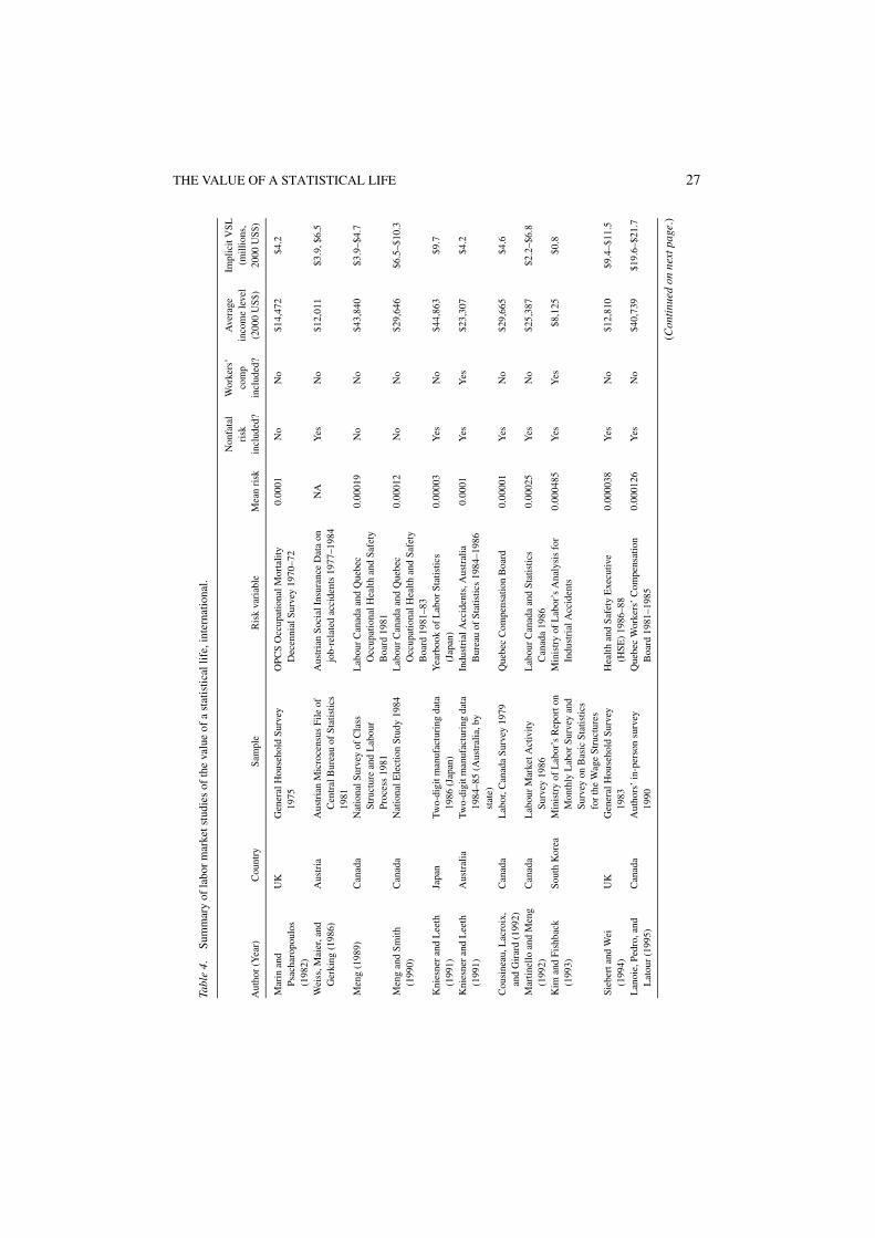
THE VALUE OF A STATISTICAL LIFE 27
Tabl
e4.
Sum
mar
yof
labo
rm
arke
tstu
dies
ofth
eva
lue
ofa
stat
istic
allif
e,in
tern
atio
nal.
Non
fata
lW
orke
rs’
Ave
rage
Impl
icit
VSL
risk
com
pin
com
ele
vel
(mill
ions
,A
utho
r(Y
ear)
Cou
ntry
Sam
ple
Ris
kva
riab
leM
ean
risk
incl
uded
?in
clud
ed?
(200
0U
S$)
2000
US$
)
Mar
inan
dPs
acha
ropo
ulos
(198
2)
UK
Gen
eral
Hou
seho
ldSu
rvey
1975
OPC
SO
ccup
atio
nalM
orta
lity
Dec
enni
alSu
rvey
1970
–72
0.00
01N
oN
o$1
4,47
2$4
.2
Wei
ss,M
aier
,and
Ger
king
(198
6)A
ustr
iaA
ustr
ian
Mic
roce
nsus
File
ofC
entr
alB
urea
uof
Stat
istic
s19
81
Aus
tria
nSo
cial
Insu
ranc
eD
ata
onjo
b-re
late
dac
cide
nts
1977
–198
4N
AY
esN
o$1
2,01
1$3
.9,$
6.5
Men
g(1
989)
Can
ada
Nat
iona
lSur
vey
ofC
lass
Stru
ctur
ean
dL
abou
rPr
oces
s19
81
Lab
our
Can
ada
and
Que
bec
Occ
upat
iona
lHea
lthan
dSa
fety
Boa
rd19
81
0.00
019
No
No
$43,
840
$3.9
–$4.
7
Men
gan
dSm
ith(1
990)
Can
ada
Nat
iona
lEle
ctio
nSt
udy
1984
Lab
our
Can
ada
and
Que
bec
Occ
upat
iona
lHea
lthan
dSa
fety
Boa
rd19
81–8
3
0.00
012
No
No
$29,
646
$6.5
–$10
.3
Kni
esne
ran
dL
eeth
(199
1)Ja
pan
Two-
digi
tman
ufac
turi
ngda
ta19
86(J
apan
)Y
earb
ook
ofL
abor
Stat
istic
s(J
apan
)0.
0000
3Y
esN
o$4
4,86
3$9
.7
Kni
esne
ran
dL
eeth
(199
1)A
ustr
alia
Two-
digi
tman
ufac
turi
ngda
ta19
84–8
5(A
ustr
alia
,by
stat
e)
Indu
stri
alA
ccid
ents
,Aus
tral
iaB
urea
uof
Stat
istic
s19
84–1
986
0.00
01Y
esY
es$2
3,30
7$4
.2
Cou
sine
au,L
acro
ix,
and
Gir
ard
(199
2)C
anad
aL
abor
,Can
ada
Surv
ey19
79Q
uebe
cC
ompe
nsat
ion
Boa
rd0.
0000
1Y
esN
o$2
9,66
5$4
.6
Mar
tinel
loan
dM
eng
(199
2)C
anad
aL
abou
rM
arke
tAct
ivity
Surv
ey19
86L
abou
rC
anad
aan
dSt
atis
tics
Can
ada
1986
0.00
025
Yes
No
$25,
387
$2.2
–$6.
8
Kim
and
Fish
back
(199
3)So
uth
Kor
eaM
inis
try
ofL
abor
’sR
epor
ton
Mon
thly
Lab
orSu
rvey
and
Surv
eyon
Bas
icSt
atis
tics
for
the
Wag
eSt
ruct
ures
Min
istr
yof
Lab
or’s
Ana
lysi
sfo
rIn
dust
rial
Acc
iden
ts0.
0004
85Y
esY
es$8
,125
$0.8
Sieb
erta
ndW
ei(1
994)
UK
Gen
eral
Hou
seho
ldSu
rvey
1983
Hea
lthan
dSa
fety
Exe
cutiv
e(H
SE)
1986
–88
0.00
0038
Yes
No
$12,
810
$9.4
–$11
.5
Lan
oie,
Pedr
o,an
dL
atou
r(1
995)
Can
ada
Aut
hors
’in
-per
son
surv
ey19
90Q
uebe
cW
orke
rs’
Com
pens
atio
nB
oard
1981
–198
50.
0001
26Y
esN
o$4
0,73
9$1
9.6–
$21.
7
(Con
tinu
edon
next
page
.)
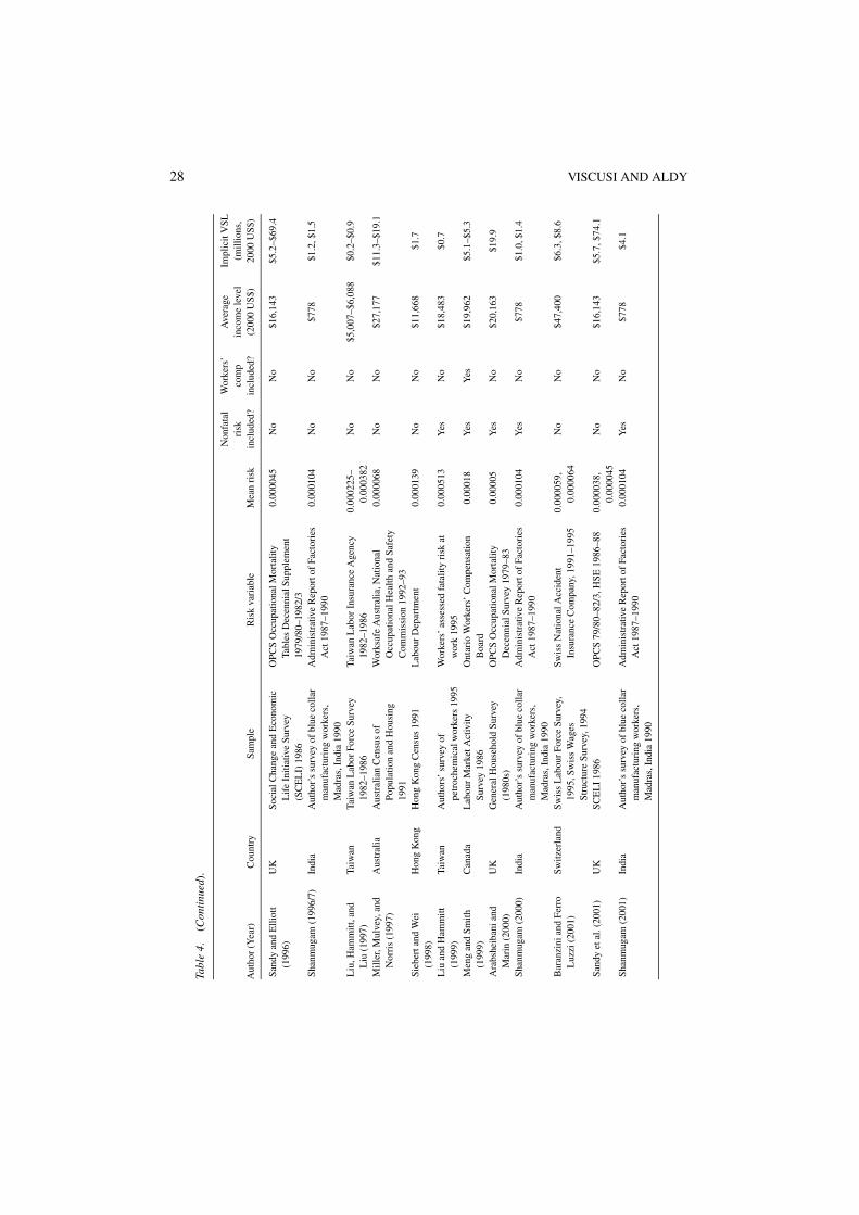
28 VISCUSI AND ALDY
Tabl
e4.
(Con
tinu
ed).
Non
fata
lW
orke
rs’
Ave
rage
Impl
icit
VSL
risk
com
pin
com
ele
vel
(mill
ions
,A
utho
r(Y
ear)
Cou
ntry
Sam
ple
Ris
kva
riab
leM
ean
risk
incl
uded
?in
clud
ed?
(200
0U
S$)
2000
US$
)
Sand
yan
dE
lliot
t(1
996)
UK
Soci
alC
hang
ean
dE
cono
mic
Lif
eIn
itiat
ive
Surv
ey(S
CE
LI)
1986
OPC
SO
ccup
atio
nalM
orta
lity
Tabl
esD
ecen
nial
Supp
lem
ent
1979
/80–
1982
/3
0.00
0045
No
No
$16,
143
$5.2
–$69
.4
Shan
mug
am(1
996/
7)In
dia
Aut
hor’
ssu
rvey
ofbl
ueco
llar
man
ufac
turi
ngw
orke
rs,
Mad
ras,
Indi
a19
90
Adm
inis
trat
ive
Rep
orto
fFa
ctor
ies
Act
1987
–199
00.
0001
04N
oN
o$7
78$1
.2,$
1.5
Liu
,Ham
mitt
,and
Liu
(199
7)Ta
iwan
Taiw
anL
abor
Forc
eSu
rvey
1982
–198
6Ta
iwan
Lab
orIn
sura
nce
Age
ncy
1982
–198
60.
0002
25–
0.00
0382
No
No
$5,0
07–$
6,08
8$0
.2–$
0.9
Mill
er,M
ulve
y,an
dN
orri
s(1
997)
Aus
tral
iaA
ustr
alia
nC
ensu
sof
Popu
latio
nan
dH
ousi
ng19
91
Wor
ksaf
eA
ustr
alia
,Nat
iona
lO
ccup
atio
nalH
ealth
and
Safe
tyC
omm
issi
on19
92–9
3
0.00
0068
No
No
$27,
177
$11.
3–$1
9.1
Sieb
erta
ndW
ei(1
998)
Hon
gK
ong
Hon
gK
ong
Cen
sus
1991
Lab
our
Dep
artm
ent
0.00
0139
No
No
$11,
668
$1.7
Liu
and
Ham
mitt
(199
9)Ta
iwan
Aut
hors
’su
rvey
ofpe
troc
hem
ical
wor
kers
1995
Wor
kers
’as
sess
edfa
talit
yri
skat
wor
k19
950.
0005
13Y
esN
o$1
8,48
3$0
.7
Men
gan
dSm
ith(1
999)
Can
ada
Lab
our
Mar
ketA
ctiv
itySu
rvey
1986
Ont
ario
Wor
kers
’C
ompe
nsat
ion
Boa
rd0.
0001
8Y
esY
es$1
9,96
2$5
.1–$
5.3
Ara
bshe
iban
iand
Mar
in(2
000)
UK
Gen
eral
Hou
seho
ldSu
rvey
(198
0s)
OPC
SO
ccup
atio
nalM
orta
lity
Dec
enni
alSu
rvey
1979
–83
0.00
005
Yes
No
$20,
163
$19.
9
Shan
mug
am(2
000)
Indi
aA
utho
r’s
surv
eyof
blue
colla
rm
anuf
actu
ring
wor
kers
,M
adra
s,In
dia
1990
Adm
inis
trat
ive
Rep
orto
fFa
ctor
ies
Act
1987
–199
00.
0001
04Y
esN
o$7
78$1
.0,$
1.4
Bar
anzi
nian
dFe
rro
Luz
zi(2
001)
Switz
erla
ndSw
iss
Lab
our
Forc
eSu
rvey
,19
95,S
wis
sW
ages
Stru
ctur
eSu
rvey
,199
4
Swis
sN
atio
nalA
ccid
ent
Insu
ranc
eC
ompa
ny,1
991–
1995
0.00
0059
,0.
0000
64N
oN
o$4
7,40
0$6
.3,$
8.6
Sand
yet
al.(
2001
)U
KSC
EL
I19
86O
PCS
79/8
0–82
/3,H
SE19
86–8
80.
0000
38,
0.00
0045
No
No
$16,
143
$5.7
,$74
.1
Shan
mug
am(2
001)
Indi
aA
utho
r’s
surv
eyof
blue
colla
rm
anuf
actu
ring
wor
kers
,M
adra
s,In
dia
1990
Adm
inis
trat
ive
Rep
orto
fFa
ctor
ies
Act
1987
–199
00.
0001
04Y
esN
o$7
78$4
.1
THE VALUE OF A STATISTICAL LIFE 29
a relatively large VSL of about $18 million, regression analyses of subsamples resulted inVSLs ranging up to $68 million (in this case, for non-manual workers). While this resultqualitatively conforms to the U.S. findings of lower VSLs for workers in higher risk jobs(see Figure 2), the magnitude of the U.K. compensating differentials seems implausiblylarge.
The results from several of the studies of the United Kingdom reveal compensating differ-entials on the order of 10 percent of total worker wage income. One regression result (with aVSL of $69 million) from Sandy and Elliott (1996) implies a compensating differential formortality risk comprising nearly 20 percent of worker wages. These risk premiums are sub-stantially larger than the compensating differentials evident in other developed countries’labor markets, even those countries with higher per capita incomes. Moreover, risk levelscannot account for the high wage share of compensating differentials as the mortality riskis lower than in many U.S. studies. The large U.K. compensating differentials may reflectcorrelation between the risk measure and other unobservables that yield substantial returnsto the worker.
After the United States, no country has been the focus of more hedonic labor marketanalyses of wage-risk tradeoffs than Canada. The Canadian studies appear to producecompensating differentials more in line with the U.S. experience than with the evidencefrom the U.K. labor market. With the exception of Lanoie, Pedro, and LaTour (1995), mostCanadian labor market VSLs fall within the range of $3–$6 million. The Lanoie et al.findings of a VSL on the order of $18 million–$20 million may reflect their data collectionmethodology. They surveyed about 200 workers in the Montreal area and solicited workers’perceptions of risk with a risk information ladder similar to that in Gegax, Gerking, andSchulze (1991), which suffered from using a truncated job risk scale that omitted most jobrisks in the U.S. economy. Analyses by Lanoie et al. with industry risk measures providedby the Quebec Compensation Board did not yield statistically significant risk coefficients,while the perceived risk measures generated these large VSLs. This result contrasts withthe findings of Cousineau, Lacroix, and Girard (1992) who found a statistically significantcompensating differential for risk using mortality risk data from the same source on a sampleof more than 30,000 Quebec workers.
With the exception of some U.K. studies, the compensating differentials estimated indeveloped country analyses tend to find risk premiums ranging between 1–2 percent of laborincome. These results are broadly consistent with the findings in the Duncan and Holmlund(1983) paper that used Swedish workers’ perceptions of danger in lieu of measured industrymortality risks. The authors estimated a statistically significant and positive compensatingwage differential for dangerous jobs on the order of about 2 percent of wages. Swedishworkers’ perceptions of danger yield comparable compensating differentials to measuredindustry mortality risk in both U.S. and European studies (see Viscusi, 1979 for an examplefrom the U.S. labor market).
Researchers have also evaluated the VSL in several of the newly industrialized countriesof Asia, including Hong Kong, South Korea, and Taiwan. Note that these countries haveon-the-job mortality risks three to five times greater than the average in Australia, the UnitedStates, and the United Kingdom. Further, the average worker earnings are two to four timeslower than labor earnings in developed countries.

30 VISCUSI AND ALDY
Kim and Fishback (1999) examined the South Korean labor market over the 1984–1990period. Unlike many of the studies in developed countries, which employ worker-leveldata, their unit of observation is at the industry level. Kim and Fishback estimate a VSL ofapproximately $0.5 million. They note that the estimated VSL is about 94 times the averageannual earnings of workers. Siebert and Wei (1998) estimate a VSL for the Hong Kongworkforce that is larger than the Korean estimate by about a factor of three. The ratio of VSLto average annual earnings for Hong Kong is about 150. These estimates are of the sameorder of magnitude as the ratio of VSL to annual earnings evident in the U.S. labor market.
Liu, Hammitt, and Liu (1997) and Liu and Hammitt (1999) estimated the wage-risk trade-off in Taiwan. The Liu, Hammitt, and Liu study focuses on all non-agricultural workerswhile Liu and Hammitt base their analysis on in-person surveys of petrochemical workers.In the former case, the authors use 3-digit industry level risk data, while the latter paperuses workers’ risk perceptions derived from a survey instrument similar to that in Gegax,Gerking, and Schulze (1991). Workers’ risk perceptions in the petrochemical industry yielda mortality risk rate about 35 percent greater than the rate published by the Taiwan LaborInsurance Agency, the data source for the Liu, Hammitt, and Liu study.26 While petrochem-ical workers face higher average mortality risk (perceived and measured) than the averagefor all non-agricultural workers in Taiwan, the higher wages and income associated withpetrochemical workers in 1995 relative to the broader workforce in the early to mid 1980sprobably explains why Liu and Hammitt estimated a VSL about twice what Liu, Hammitt,and Liu found.
Estimates for the Indian labor market yield a value of a statistical life greater than theVSLs in other developing countries despite the fact that per capita income in India isan order of magnitude smaller than in these countries. Shanmugam (1996/1997, 1997,2000, 2001) assessed the wage-risk tradeoff in a variety of studies using survey data ofmanufacturing workers in Madras, India in 1990. The VSL estimates from these studiesrange by nearly a factor of four, even though they reflect the same wage and risk data,illustrating how a variety of econometric specifications can produce in some cases a range ofresults.
5. The implicit value of a statistical injury: U.S. and international estimates
Complementing the research on the returns to bearing fatal risks in the workplace, a signif-icant number of studies have evaluated the risk premium associated with bearing nonfataljob risks. The hedonic labor market studies of nonfatal risk employ the same econometricapproach as used for mortality risk. As discussed above, some studies that attempt to esti-mate jointly the effects of fatal and nonfatal risks on workers’ wages do not find significanteffects of risk on wages for at least one of the risk measures. Fatal risk is highly correlatedwith nonfatal risk, so joint estimation may result in large standard errors due to collinearity.Omitting one of these variables when estimating the other could result in an upwardly biasedestimate of the return to that type of risk.
Table 5 summarizes 31 studies from the U.S. labor market (Table 5(a)) and 8 studiesof labor markets outside of the United States (Table 5(b)) that have found statisticallysignificant influences of nonfatal job risk on wages. These studies employ three different

THE VALUE OF A STATISTICAL LIFE 31
Tabl
e5(
a).
Sum
mar
yof
labo
rm
arke
tstu
dies
ofth
eva
lue
ofst
atis
tical
inju
ry,U
nite
dSt
ates
.
Wor
kers
’A
vera
geIm
plic
itva
lue
ofM
ean
Fata
lris
kco
mp
inco
me
leve
la
stat
istic
alin
jury
Aut
hor
(Yea
r)Sa
mpl
eR
isk
vari
able
inju
ryri
skin
clud
ed?
incl
uded
?(2
000
US$
)(2
000
US$
)
Smith
(197
4)C
urre
ntPo
pula
tion
Surv
ey(C
PS)
1967
,Cen
sus
ofM
anuf
actu
res
1963
,U.S
.C
ensu
s19
60,E
mpl
oym
ent
and
Ear
ning
s19
63
Bur
eau
ofL
abor
Stat
istic
s(B
LS)
1966
,196
7N
AY
es,s
igni
fican
tN
o$2
9,02
9−$
30,9
34
Smith
(197
6)C
PS19
67,1
973
BL
S19
66,1
967,
1970
NA
Yes
,sig
nific
ant
No
$31,
027
Non
fata
linj
ury
coef
ficie
ntno
tsig
nific
ant
Vis
cusi
(197
8a,1
979)
Surv
eyof
Wor
king
Con
ditio
ns,
1969
–197
0(S
WC
)B
LS
non-
fata
linj
ury
rate
1969
(pre
-OSH
A)
0.03
2Y
es,s
igni
fican
tN
o$3
1,84
2$2
5,69
3–$4
9,44
2
Vis
cusi
(197
8b)
SWC
1969
–197
0B
LS
non-
fata
linj
ury
rate
1969
(pre
-OSH
A)
0.03
2N
oN
o$3
2,67
5$6
1,53
7–$6
3,24
1
McL
ean,
Wen
dlin
g,an
dN
eerg
aard
(197
8)
Wis
cons
inC
ensu
s19
70W
isco
nsin
Wor
kers
’C
ompe
nsat
ion
acci
dent
data
1970
0.05
No
No
$34,
414
$141
,659
Vis
cusi
(198
1)Pa
nelS
tudy
ofIn
com
eD
ynam
ics
(PSI
D)
1976
BL
Sno
n-fa
tali
njur
yra
te19
760.
032
Yes
,sig
nific
ant
No
$22,
618
$59,
238
Ols
on(1
981)
CPS
1978
BL
Sto
tall
ostw
orkd
ayac
cide
ntra
te19
730.
035
Yes
,sig
nific
ant
No
$36,
151
$24,
009–
$32,
304
Free
man
and
Med
off
(198
1)C
PSM
ay19
73–1
975
BL
Sm
ean
lost
wor
kday
spe
rw
orke
r19
72–1
974
0.70
1N
oN
oN
AN
otre
port
ed—
can’
tcal
cula
te(p
ositi
vean
dst
atis
tical
lysi
gnifi
cant
)L
eigh
(198
1)PS
ID19
74,Q
ES
1977
BL
Sin
jury
rate
s19
74N
AY
es,n
otsi
gnifi
cant
No
NA
Not
repo
rted
—ca
n’tc
alcu
late
(pos
itive
and
stat
istic
ally
sign
ifica
nt)
But
ler
(198
3)S.
C.w
orke
rs’
com
pens
atio
nda
ta19
40–6
9S.
C.w
orke
rs’
com
pens
atio
ncl
aim
sda
ta.0
61(c
laim
sra
te)
No
Yes
$22,
713
$936
/day
or$1
6,84
8fo
ran
18-d
ayin
jury
Dor
sey
and
Wal
zer
(198
3)C
PSM
ay19
78B
LS
nonf
atal
lost
wor
kday
inju
ryin
cide
nce
rate
1976
0.03
Yes
,som
esp
ecifi
catio
nsY
es$2
1,63
6$6
0,58
1,$6
9,23
5
Smith
(198
3)C
PS19
78B
LS
Wor
kIn
jury
Rat
e0.
078
No
No
$32,
488
$35,
485
(Con
tinu
edon
next
page
.)
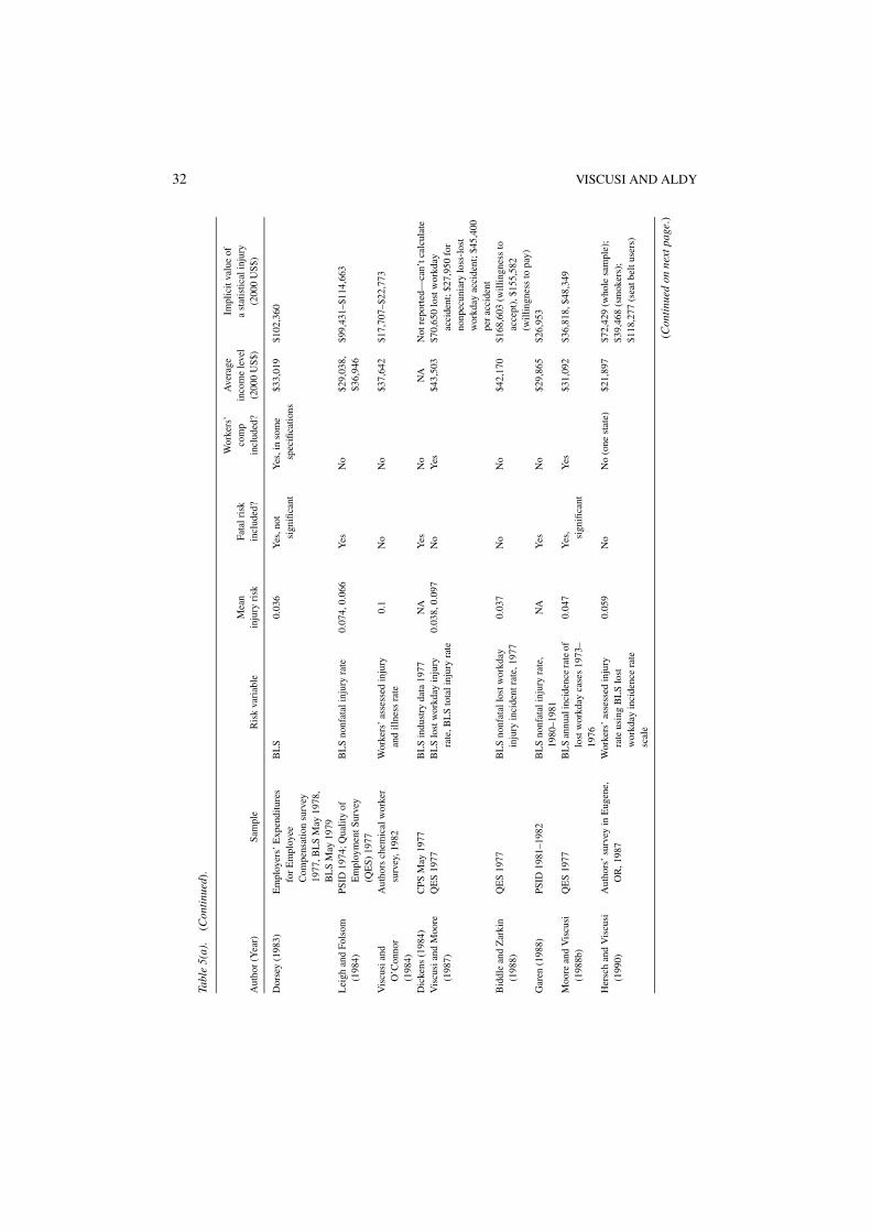
32 VISCUSI AND ALDY
Tabl
e5(
a).
(Con
tinu
ed).
Wor
kers
’A
vera
geIm
plic
itva
lue
ofM
ean
Fata
lris
kco
mp
inco
me
leve
la
stat
istic
alin
jury
Aut
hor
(Yea
r)Sa
mpl
eR
isk
vari
able
inju
ryri
skin
clud
ed?
incl
uded
?(2
000
US$
)(2
000
US$
)
Dor
sey
(198
3)E
mpl
oyer
s’E
xpen
ditu
res
for
Em
ploy
eeC
ompe
nsat
ion
surv
ey19
77,B
LS
May
1978
,B
LS
May
1979
BL
S0.
036
Yes
,not
sign
ifica
ntY
es,i
nso
me
spec
ifica
tions
$33,
019
$102
,360
Lei
ghan
dFo
lsom
(198
4)PS
ID19
74;Q
ualit
yof
Em
ploy
men
tSur
vey
(QE
S)19
77
BL
Sno
nfat
alin
jury
rate
0.07
4,0.
066
Yes
No
$29,
038,
$36,
946
$99,
431–
$114
,663
Vis
cusi
and
O’C
onno
r(1
984)
Aut
hors
chem
ical
wor
ker
surv
ey,1
982
Wor
kers
’as
sess
edin
jury
and
illne
ssra
te0.
1N
oN
o$3
7,64
2$1
7,70
7–$2
2,77
3
Dic
kens
(198
4)C
PSM
ay19
77B
LS
indu
stry
data
1977
NA
Yes
No
NA
Not
repo
rted
—ca
n’tc
alcu
late
Vis
cusi
and
Moo
re(1
987)
QE
S19
77B
LS
lost
wor
kday
inju
ryra
te,B
LS
tota
linj
ury
rate
0.03
8,0.
097
No
Yes
$43,
503
$70,
650
lost
wor
kday
acci
dent
;$27
,950
for
nonp
ecun
iary
loss
-los
tw
orkd
ayac
cide
nt;$
45,4
00pe
rac
cide
ntB
iddl
ean
dZ
arki
n(1
988)
QE
S19
77B
LS
nonf
atal
lost
wor
kday
inju
ryin
cide
ntra
te,1
977
0.03
7N
oN
o$4
2,17
0$1
68,6
03(w
illin
gnes
sto
acce
pt),
$155
,582
(will
ingn
ess
topa
y)G
aren
(198
8)PS
ID19
81–1
982
BL
Sno
nfat
alin
jury
rate
,19
80–1
981
NA
Yes
No
$29,
865
$26,
953
Moo
rean
dV
iscu
si(1
988b
)Q
ES
1977
BL
San
nual
inci
denc
era
teof
lost
wor
kday
case
s19
73–
1976
0.04
7Y
es, sign
ifica
ntY
es$3
1,09
2$3
6,81
8,$4
8,34
9
Her
sch
and
Vis
cusi
(199
0)A
utho
rs’
surv
eyin
Eug
ene,
OR
,198
7W
orke
rs’
asse
ssed
inju
ryra
teus
ing
BL
Slo
stw
orkd
ayin
cide
nce
rate
scal
e
0.05
9N
oN
o(o
nest
ate)
$21,
897
$72,
429
(who
lesa
mpl
e);
$39,
468
(sm
oker
s);
$118
,277
(sea
tbel
tuse
rs)
(Con
tinu
edon
next
page
.)
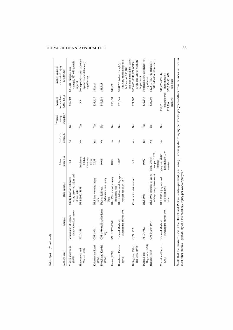
THE VALUE OF A STATISTICAL LIFE 33Ta
ble
5(a)
.(C
onti
nued
).
Wor
kers
’A
vera
geIm
plic
itva
lue
ofM
ean
Fata
lris
kco
mp
inco
me
leve
la
stat
istic
alin
jury
Aut
hor
(Yea
r)Sa
mpl
eR
isk
vari
able
inju
ryri
skin
clud
ed?
incl
uded
?(2
000
US$
)(2
000
US$
)
Vis
cusi
and
Eva
ns(1
990)
Vis
cusi
and
O’C
onno
rch
emic
alw
orke
rsu
rvey
Util
ityfu
nctio
nes
timat
esus
ing
asse
ssed
inju
ryan
dill
ness
rate
0.1
No
No
$37,
802
$23,
781
(mar
gina
lris
kch
ange
);$3
7,03
0(c
erta
inin
jury
)H
amer
mes
han
dW
olfe
(199
0)PS
ID19
81B
LS
1980
,198
1In
cide
nce:
0.04
76;
Dur
atio
n:0.
1571
No
Yes
NA
Not
repo
rted
—ca
n’tc
alcu
late
(pos
itive
and
stat
istic
ally
sign
ifica
nt)
Kni
esne
ran
dL
eeth
(199
1)C
PS19
78B
LS
lost
wor
kday
inju
ryra
te0.
055
Yes
Yes
$33,
627
$60,
624
Fren
chan
dK
enda
ll(1
992)
CPS
1980
(rai
lroa
din
dust
ryon
ly)
Fede
ralR
ailr
oad
Adm
inis
trat
ion
Inju
ryR
ate
0.04
8N
oN
o$4
6,28
4$4
8,92
8
Fair
ris
(199
2)SW
C19
69–1
970
BL
S19
69in
dust
ryin
jury
freq
uenc
yra
te0.
032
No
No
$33,
850
$49,
290
Her
sch
and
Pick
ton
(199
5)N
atio
nalM
edic
alE
xpen
ditu
reSu
rvey
1987
BL
Sto
tall
ostw
orkd
ays
per
wor
ker
per
year
1987
0.70
2†N
oN
o$2
6,34
5$1
20,7
09(w
hole
sam
ple)
;$1
55,4
53(n
onsm
oker
-sea
tbe
ltus
ers)
;$83
,186
(sm
oker
-non
seat
belt
user
s)D
illin
gham
,Mill
er,
and
Lev
y(1
996)
QE
S19
77C
onst
ruct
edri
skm
easu
reN
AY
esN
o$2
4,26
7$1
55,4
35–$
242,
671
WT
Pto
avoi
don
eye
arof
wor
klif
eim
pair
men
tD
orm
anan
dH
agst
rom
(199
8)PS
ID19
82B
LS
1981
0.05
2Y
esY
es$3
2,24
3N
onfa
tali
njur
yco
effic
ient
not
sign
ifica
ntH
ersc
h(1
998)
CPS
Mar
ch19
94B
LS
1993
(num
ber
ofca
ses
ofda
ysaw
ayfr
omw
ork)
0.02
9w
hole
sam
ple;
0.02
2fe
mal
es
No
No
$28,
004
$22,
810–
$33,
723
(fem
ales
);$1
2,14
6–$3
6,19
2(m
ales
)
Vis
cusi
and
Her
sch
(200
1)N
atio
nalM
edic
alE
xpen
ditu
reSu
rvey
1987
BL
S19
87in
jury
rate
and
lost
wor
kday
sra
te
Inju
ryra
te:0
.042
nons
mok
er;0
.49
smok
er
No
No
$31,
651
(non
smok
ers)
;$2
8,31
6(s
mok
ers)
$47,
476–
$59,
144
(non
smok
ers)
;$2
0,75
5–$3
1,02
8(s
mok
ers)
† Not
eth
atth
em
easu
reus
edin
the
Her
sch
and
Pick
ton
stud
y—pr
obab
ility
oflo
sing
1w
orkd
aydu
eto
inju
rype
rw
orke
rpe
rye
ar—
diff
ers
from
the
mea
sure
used
inm
osto
ther
stud
ies—
prob
abili
tyof
alo
stw
orkd
ayin
jury
per
wor
ker
per
year
.
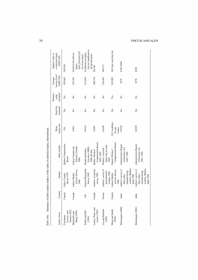
34 VISCUSI AND ALDY
Tabl
e5(
b).
Sum
mar
yof
labo
rm
arke
tstu
dies
ofth
eva
lue
ofst
atis
tical
inju
ry,i
nter
natio
nal.
Wor
kers
’A
vera
geIm
plic
itva
lue
ofM
ean
Fata
lris
kco
mp
inco
me
Lev
ela
stat
istic
alin
jury
Aut
hor
(Yea
r)C
ount
rySa
mpl
eR
isk
vari
able
inju
ryri
skin
clud
ed?
incl
uded
?(2
000
US$
)(2
000
US$
)
Cou
sine
au,
Lac
roix
,and
Gir
ard
(199
2)
Can
ada
Lab
or,C
anad
aSu
rvey
1979
Que
bec
Com
pens
atio
nB
oard
NA
Yes
No
$29,
665
$38,
104
Mar
tinel
loan
dM
eng
(199
2)C
anad
aL
abou
rM
arke
tA
ctiv
itySu
rvey
1986
Lab
our
Can
ada
and
Stat
istic
sC
anad
a19
86
0.06
3Y
esN
o$2
5,38
7$1
0,81
5-$1
4,45
6fo
rin
jury
;$1
61,2
10-$
191,
027
for
seve
rein
jury
Sieb
erta
ndW
ei(1
994)
UK
Gen
eral
Hou
seho
ldSu
rvey
1983
Hea
lthan
dSa
fety
Exe
cutiv
e(H
SE)
1986
–88
data
0.01
43Y
esN
o$1
2,81
0C
oeffi
cien
ton
inju
ryri
skno
tsig
nific
anti
nal
lspe
cific
atio
nsL
anoi
e,Pe
dro,
and
Lat
our
(199
5)C
anad
aA
utho
rs’
in-p
erso
nsu
rvey
1990
Que
bec
Wor
kers
’C
ompe
nsat
ion
Boa
rd19
81–1
985
0.09
9Y
esN
o$4
0,73
9$8
,148
Liu
and
Ham
mitt
(199
9)Ta
iwan
Aut
hors
’su
rvey
ofpe
troc
hem
ical
wor
kers
1999
Wor
kers
’as
sess
edin
jury
risk
atw
ork
1995
0.01
09Y
esN
o$1
8,48
3$4
9,71
7
Men
gan
dSm
ith(1
999)
Can
ada
Lab
our
Mar
ket
Act
ivity
Surv
ey19
86
Ont
ario
Wor
kers
’C
ompe
nsat
ion
Boa
rd3.
01–w
orkd
ays
lost
per
wor
ker
Yes
Yes
$19,
962
$423
per
wor
kda
ylo
st
Shan
mug
am(2
000)
Indi
aA
utho
r’s
surv
eyof
blue
colla
rm
anuf
actu
ring
wor
kers
,Mad
ras,
Indi
a19
90
Adm
inis
trat
ive
Rep
ort
ofFa
ctor
ies
Act
1987
–199
0
0.07
29Y
esN
o$7
78$1
50–$
560
Shan
mug
am(2
001)
Indi
aA
utho
r’s
surv
eyof
blue
colla
rm
anuf
actu
ring
wor
kers
,Mad
ras,
Indi
a19
90
Adm
inis
trat
ive
Rep
ort
ofFa
ctor
ies
Act
1987
–199
0
0.07
29Y
esN
o$7
78$3
50

THE VALUE OF A STATISTICAL LIFE 35
measures of nonfatal job risks: the overall injury rate, the rate of injuries severe enough toresult in a lost workday, and the rate of total lost workdays. Studies using different mea-sures of nonfatal job risks will generate different risk premiums because the return to thefrequency of injuries (the injury rate) will usually differ from the return to the severityof injuries (lost workdays rate). In two studies with specialized data, Butler (1983) con-structed an injury rate from South Carolina workers’ compensation claims, restricting hisrisk measure to only the more serious work accidents and French and Kendall (1992) andFrench (1990) constructed an injury rate for railroad workers based on data collected by theFederal Railroad Administration. As an alternative to these objective measures of risk, Vis-cusi and O’Connor (1984) and Hersch and Viscusi (1990) used workers’ own assessmentsof risk with risk scales based on the BLS injury rate and the BLS lost workday accidentrate, respectively. These authors estimated comparable wage-risk tradeoffs based on sub-jective risk perception as the other studies based on objectively measured industry-levelrisk.
These value of statistical injury studies yield a wide range of estimates, reflecting boththe differences in the risk measures used as well as whether mortality risk is included in theresults. While several studies have very high values of injury, such as McLean, Wendling,and Neergaard (1978), Leigh and Folsum (1984), and Biddle and Zarkin (1988), moststudies have estimates in the range of $20,000–$70,000 per injury.
The value of statistical injury appears to vary with workers’ preferences over risk, con-sistent with some of the findings based on the mortality risk literature. As a proxy forrisk attitudes, several studies have used information about workers’ behavior outside of theworkplace, such as smoking status and seatbelt use, to identify the effect of risk preferenceson wage-risk tradeoffs. Hersch and Viscusi (1990), Hersch and Pickton (1995), and Viscusiand Hersch (2001) all found that smokers have lower injury risk premiums than do non-smokers. Hersch and Viscusi as well as Hersch and Pickton also found that individuals whodo not wear seatbelts have lower injury risk premiums than do individuals who regularlywear seatbelts.
The study by Hersch (1998) is of particular interest because it used gender-specific riskmeasures. Many previous studies had focused on male samples only because estimatesusing industry-based measures often failed to yield significant risk premiums for women.Researchers hypothesized that women did not work in risky jobs that would pose healthand safety risks. The estimates by Hersch indicate that the nonfatal injury risk for womenis over two-thirds the size of that for men and that the wage-injury risk tradeoff rates aresimilar for men and women.
The evidence outside of the United States, while based on a smaller set of studies, alsoindicates significant injury risk premiums. For example, the Cousineau, Lacroix, and Girard(1992) result falls within the U.S. range of about $20,000–$70,000. However, several otherCanadian labor market studies provide some estimates that are lower, such as Martinelloand Meng (1992) and Meng and Smith (1999). The value of statistical injury estimatesfor India are much smaller, likely reflecting the effect of per capita income on wage-risktradeoffs. The low values of statistical injury are somewhat surprising given that these samestudies generated fairly large values of statistical life.
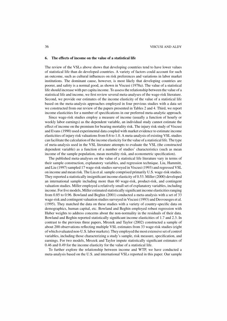
36 VISCUSI AND ALDY
6. The effects of income on the value of a statistical life
The review of the VSLs above shows that developing countries tend to have lower valuesof statistical life than do developed countries. A variety of factors could account for suchan outcome, such as cultural influences on risk preferences and variations in labor marketinstitutions. The dominant cause, however, is most likely that developing countries arepoorer, and safety is a normal good, as shown in Viscusi (1978a). The value of a statisticallife should increase with per capita income. To assess the relationship between the value of astatistical life and income, we first review several meta-analyses of the wage-risk literature.Second, we provide our estimates of the income elasticity of the value of a statistical lifebased on the meta-analysis approaches employed in four previous studies with a data setwe constructed from our review of the papers presented in Tables 2 and 4. Third, we reportincome elasticities for a number of specifications in our preferred meta-analytic approach.
Since wage-risk studies employ a measure of income (usually a function of hourly orweekly labor earnings) as the dependent variable, an individual study cannot estimate theeffect of income on the premium for bearing mortality risk. The injury risk study of Viscusiand Evans (1990) used experimental data coupled with market evidence to estimate incomeelasticities of injury risk valuations from 0.6 to 1.0. A meta-analysis of existing VSL studiescan facilitate the calculation of the income elasticity for the value of a statistical life. The typeof meta-analysis used in the VSL literature attempts to evaluate the VSL (the constructeddependent variable) as a function of a number of studies’ characteristics (such as meanincome of the sample population, mean mortality risk, and econometric specification).
The published meta-analyses on the value of a statistical life literature vary in terms oftheir sample construction, explanatory variables, and regression technique. Liu, Hammitt,and Liu (1997) sampled 17 wage-risk studies surveyed in Viscusi (1993) and regressed VSLon income and mean risk. The Liu et al. sample comprised primarily U.S. wage-risk studies.They reported a statistically insignificant income elasticity of 0.53. Miller (2000) developedan international sample including more than 60 wage-risk, product-risk, and contingentvaluation studies. Miller employed a relatively small set of explanatory variables, includingincome. For five models, Miller estimated statistically significant income elasticities rangingfrom 0.85 to 0.96. Bowland and Beghin (2001) conducted a meta-analysis with a set of 33wage-risk and contingent valuation studies surveyed in Viscusi (1993) and Desvousges et al.(1995). They matched the data on these studies with a variety of country-specific data ondemographics, human capital, etc. Bowland and Beghin employed robust regression withHuber weights to address concerns about the non-normality in the residuals of their data.Bowland and Beghin reported statistically significant income elasticities of 1.7 and 2.3. Incontrast to the previous three papers, Mrozek and Taylor (2002) constructed a sample ofabout 200 observations reflecting multiple VSL estimates from 33 wage-risk studies (eightof which evaluated non-U.S. labor markets). They employed the most extensive set of controlvariables, including those characterizing a study’s sample, risk measure, specification, andearnings. For two models, Mrozek and Taylor impute statistically significant estimates of0.46 and 0.49 for the income elasticity for the value of a statistical life.
To further explore the relationship between income and WTP, we have conducted ameta-analysis based on the U.S. and international VSLs reported in this paper. Our sample

THE VALUE OF A STATISTICAL LIFE 37
includes the VSLs for 49 studies presented in Tables 2 and 4.27 Each study yields oneobservation. Refer to the appendix for a description of the explanatory variables and theirsummary statistics.
We replicated the results from the four previous meta-analysis studies with our wage-riskstudy sample (see Table 6). For the Liu, Hammitt, and Liu (1997) model, we replicated theireconometric specification exactly. Miller (2000) reported a number of specifications. Onlymodel 3 of Miller’s meta-analysis employed per capita incomes converted to US dollars on apurchasing power parity (PPP) basis. Because we constructed all VSLs and annual incomesbased on a PPP basis, we replicated his model 3. Note that dummy variables for contingentvaluation surveys and wage-risk studies are unnecessary since our data set comprises onlywage-risk studies. Bowland and Beghin (2001) reported results for linear, log-linear, andtrans-log specifications. While they presented very limited information about most of theircontrol variables, we have attempted to replicate their set of controls. We do not haveinformation on the average age of the sample used in the VSL studies, and we have omittedthis variable from our specification. We have proxied for percent of sample in union-affiliatedjobs by accounting for whether the VSL study includes union membership as a control andwhether the VSL is union-based. Our studies do not provide average educational attainment,so we have proxied these values with national annual average educational attainment forthe over-25 population from Barro and Lee (1996). We replicated the robust regressionswith Huber weights. Our analyses with log-linear and trans-log specifications, however,yielded insignificant coefficients on income. We only present the results from the linearrobust regression model with our data. Mrozek and Taylor (2002) reported results fromfour specification models. We have focused on their model 2 since model 1 yields virtuallyidentical results and models 3 and 4 are U.S.-specific. We have included all the controlvariables that Mrozek and Taylor report, with the exception of a dummy variable for whitecollar-based VSLs. Our sample does not include any white collar-based VSLs.
Three of the four specifications yield statistically significant coefficients on the relevantincome variable. We found a comparable point estimate with much narrower bounds thanLiu et al. with their specification, perhaps reflecting our larger sample, as their sample isessentially a subset of our sample. We found a smaller coefficient on the income variablethan Miller with his specification, although a very comparable coefficient on the Societyof Actuaries risk data dummy variable (equivalent to Miller’s variable label “risk beyondworkplace” with our data). For comparison with Bowland and Beghin’s choice of using“marginal willingness to pay” as their dependent variable (apparently equivalent to theVSL expressed in terms of hourly wage instead of annual labor income), we modifiedour dependent variable accordingly. Imputing the income elasticity with the linear incomecoefficient in this model requires the sample means of VSL ($3,350 per hour worked,assuming 2000 hours worked per year and $6.7 million VSL) and income ($26,006). With23 explanatory variables and only 41 observations, the Mrozek and Taylor specificationyields very few precise coefficient estimates.
While the reported income elasticities from these four studies vary by a factor of 3, theimputed elasticity point estimates with our data set cover a much smaller range (see Table 7).With these studies’ specifications, we found income elasticities from about 0.5 to 0.6. The95 percent confidence interval upper bounds fall below 1.0 for two of the three statistically

38 VISCUSI AND ALDY
Table 6. Replication of published meta-analyses with Viscusi-Aldy data.
Viscusi-Aldy Viscusi-AldyVersion of Liu Viscusi-Aldy Version of Bowland- Viscusi-Aldy Versionet al. (1997) Version of Miller Beghin (2001) of Mrozek-Taylor
Eq. (2) (2000) Model 3 linear model (2002) Model 2Variable (1) (2) (3) (4)
Dependent VSL (expressed invariable log (VSL) log (VSL) per hour terms) log (VSL)
log(Income) 0.51∗ 0.53∗ – –
(0.15) (0.17)
Income – – 0.078∗∗ –
(0.031)
Hourly wage – – – 0.040
(0.026)
Mean risk −0.015∗ – −19.34∗∗ −0.16∗∗∗
(0.0057) (8.56) (0.075)
Mean risk squared – – – 0.0019
(0.0015)
Union × mean risk – – – 0.22∗∗∗
(0.11)
Dillingham risk – – – −0.32
(0.58)
Society ofActuaries risk
– −1.29∗ – –
(0.28)
BLS risk – – 1445.18∗∗ –
(591.47)
NIOSH risk – – – 0.27
(0.40)
Education level – – −157.14 –
(192.32)
Unemployment rate – – – 0.045
(0.048)
U.S. national data – – – 0.31
(0.82)
Non-U.S. study – – – −0.0048
(0.81)
Union VSL – – 2995.05∗ −0.42
(1086.09) (0.90)
Union dummyvariable
– – 1000.76 0.43
(638.37) (0.40)
Male only sample – – −588.20 –
(600.82)
(Continued on next page.)
THE VALUE OF A STATISTICAL LIFE 39
Table 6. (Continued).
Viscusi-Aldy Viscusi-AldyVersion of Liu Viscusi-Aldy Version of Bowland- Viscusi-Aldy Versionet al. (1997) Version of Miller Beghin (2001) of Mrozek-Taylor
Eq. (2) (2000) Model 3 linear model (2002) Model 2Variable (1) (2) (3) (4)
Dependent VSL (expressed invariable log (VSL) log (VSL) per hour terms) log (VSL)
Blue collar sample – – −812.78 −0.68
(644.54) (0.49)
Quadratic risk – – – 0.54
(0.33)
Morbidity variableincluded
– – – 0.11
(0.32)
log(Dependentvariable)
– – – −0.24
(0.36)
Regional dummyvariable
– – −757.70 0.16
(601.16) (0.35)
Urban dummyvariable
– – −65.91 0.12
(804.50) (0.41)
Workers’compensation
– – – 0.10
(0.45)
Wage in aftertax terms
– – – −0.29
(0.50)
Industry dummyvariable
– – – 0.081
(0.27)
Occupation dummyvariable
– – – 0.0039
(0.20)
No occupationdummy variable
– 0.48 – –
(0.33)
Job characteristicsdummy variable
– – – −0.021
(0.51)
Constant 10.56∗ 9.80∗ 1935.54 15.68∗
(1.49) (1.78) (1506.92) (1.39)
R2 0.37 0.27 – 0.83
n 46 49 45 41
Specifications (1), (2), and (4) estimated with ordinary least squares.Specification (3) estimated with robust regression with Huber weights.Robust (White) standard errors are presented in parentheses for specifications (1), (2), and (4).Asymptotic standard errors presented in parentheses for specification (3).∗Indicates statistical significance at 1 percent level.∗∗Indicates statistical significance at 5 percent level.∗∗∗Indicates statistical significance at 10 percent level.

40 VISCUSI AND ALDY
Table 7. Income elasticity of willingness-to-pay to reduce mortality risk.
Paper (Model) Reported elasticity in authors’ papers Viscusi-Aldy version
Liu, Hammitt, and Liu (1997) 0.53 0.51∗(Eq. (2)) (0.21–0.80)
Miller (2000) 0.89∗ 0.53∗(Model 3) (0.20–0.86)
Mrozek and Taylor (2002) 0.46∗∗ 0.52(Model 2) (−0.18–1.22)
Bowland and Beghin (2001) 1.66∗ 0.61∗∗(linear model) (0.11–1.10)
Ranges in parentheses represent the 95 percent confidence interval around the point estimate for theincome elasticity.∗Indicates elasticity is based on coefficient that is statistically significant at 1 percent level.∗∗Indicates elasticity is based on coefficient that is statistically significant at 5 percent level.
significant income elasticities estimated by the specifications outlined in these four studies.The apparently large variation in income elasticities in this literature apparently reflectsauthors’ choices of studies for inclusion more so than choices over control variables andregression techniques.
To augment the replications of previously published meta-analysis specifications, weevaluated a large number of specifications. Based on the existing literature, we focused ontwo regression techniques, ordinary least squares and robust regression with Huber weights.We have varied the control variables from as few as 3 to as many as 18, recognizing thatcoefficient estimates’ precision will decline with the length of the right-hand side of theregression equations given our sample size. We chose to include explanatory variables ofthe following types: income and mean risk (common to all specifications), type of riskmeasure, and specification variables.
The estimated coefficient on the income variable is rather stable across both regressiontechniques and for a wide variation in the number of control variables (see Table 8). Forthe OLS specifications, the income elasticity varies from 0.49 to 0.60. The 95 percentconfidence intervals never range below 0.2 and never exceed 0.95. For the robust regressionspecifications, the income elasticity varies from 0.46 to 0.48. The 95 percent confidenceintervals never fall below 0.15 and never exceed 0.78.28 The income coefficients in allspecifications are statistically significant at the 1 percent level.
Based on the approximately 50 wage-risk studies from 10 countries, we can concludefrom these results that the income elasticity for the value of a statistical life is less than 1.0.Across a number of specifications with our data, our point estimates of the income elasticityrange between about 0.5 and 0.6. Note that in none of our specifications did the incomeelasticity’s 95 percent confidence interval upper bound exceed 1.0.
Current practice by regulatory agencies is effectively in line with these findings. The U.S.EPA (1999) accounted for income growth into the 22nd century in monetizing the long-term mortality risk reduction benefits from stratospheric ozone protection.29 In a regulatorycontext, the U.S. EPA (2000b) also accounted for income growth over a thirty-year period inmonetizing the mortality risk reduction benefits from reduced particulate matter pollution

THE VALUE OF A STATISTICAL LIFE 41
Table 8. Regression models for Viscusi-Aldy meta-analysis.
Variable (1) (2) (3) (4) (5) (6)
Regression Robust with Robust with Robust withtechnique OLS OLS OLS Huber weights Huber weights Huber weights
log(Income) 0.51∗ 0.49∗ 0.60∗ 0.48∗ 0.46∗ 0.47∗(0.15) (0.13) (0.16) (0.12) (0.11) (0.15)
Mean risk −0.015∗∗ −0.053∗ −0.045∗ −0.029∗ −0.090∗ −0.11∗(0.0057) (0.011) (0.015) (0.0061) (0.018) (0.029)
Mean risk squared – 0.00022∗ 0.00016∗ – 0.00065∗ 0.0010∗∗(0.000052) (0.000055) (0.00019) (0.00035)
Society of Actuaries – – 0.50 – – Droppedrisk (0.87)
NIOSH risk – – 0.50 – – 0.56(0.41) (0.41)
Subjective – – −0.69 – – −0.16(0.78) (0.98)
Union dummy – – 0.44 – – 0.50variable (0.32) (0.30)
Male only sample – – 0.24 – – 0.36(0.36) (0.34)
Blue collar sample – – −0.016 – – −0.23(0.31) (0.33)
Quadratic risk – – 0.092 – – 0.20(0.27) (0.34)
Morbidity variable – – 0.55∗∗∗ – – 0.62∗∗included (0.30) (0.30)
log(Dependent – – 0.17 – – 0.13variable) (0.31) (0.41)
Regional dummy – – −0.16 – – 0.16variable (0.25) (0.31)
Urban dummy – – 0.38 – – 0.087variable (0.29) (0.39)
Workers’ – – −0.57 – – −0.28compensation (0.33) (0.38)
Industry dummy – – −0.46 – – −0.37variable (0.27) (0.28)
Occupation dummy – – −0.45 – – −0.24variable (0.31) (0.33)
Constant 10.56∗ 11.22∗ 9.58∗ 11.05∗ 11.83∗ 11.22∗(1.49) (1.30) (1.82) (1.23) (1.12) (1.68)
R2 0.37 0.55 0.72 – – –
(Continued on next page.)

42 VISCUSI AND ALDY
Table 8. (Continued).
Regression Robust with Robust with Robust withtechnique OLS OLS OLS Huber weights Huber weights Huber weights
n 46 46 46 45 45 44
Income elasticity (95% 0.51 0.49 0.60 0.48 0.46 0.47confidence interval) (0.21–0.80) (0.23–0.75) (0.27–0.94) (0.23–0.73) (0.24–0.69) (0.15–0.78)
Mean predicted VSL, 5.0 5.4 5.9 5.5 5.9 6.2full sample (millions (3.4–7.4) (3.7–7.8) (2.7–13.9) (4.1–7.5) (4.4–8.1) (2.5–15.7)2000 US$) (95%confidence interval)
Mean predicted VSL, 5.5 5.8 6.9 6.1 6.3 7.6U.S. sample (millions (3.8–8.1) (4.1–8.3) (3.1–16.2) (4.6–8.2) (4.8–8.4) (3.0–19.4)2000 US$) (95%confidence interval)
Dependent variable: log(VSL).Robust (White) standard errors presented in parentheses for specifications 1–3.Asymptotic standard errors presented in parentheses for specifications 4–6.∗Indicates statistical significance at 1 percent level.∗∗Indicates statistical significance at 5 percent level.∗∗∗Indicates statistical significance at 10 percent level.Note: Estimation with robust standard errors clustered by wage data source yields same significance levels, withthe exception of Mean Risk in (1) and (3) and Mean Risk Squared in (3), which are all significant at the 2 percentlevel, and the industry dummy variable in (3) which is significant at the 8 percent level.
associated with the diesel sulfur standard for heavy-duty trucks. In both these cases, theU.S. EPA employed an income elasticity of 0.4 and conducted sensitivity analyses witha low-end elasticity of 0.1 and a high-end elasticity of 1.0. If our results for the incomeelasticity apply over time, the point estimate chosen by the EPA is reasonable, althoughmore narrow bounds may be appropriate for the sensitivity analysis.
The meta-analysis regressions can also serve to characterize some of the uncertaintyin value of a statistical life estimates. We constructed the mean predicted VSL valuespresented in the last two rows of Table 8 by first using the estimated coefficients from themeta-analysis regressions to predict the natural logarithm of VSL for each study. Then weconverted each predicted log(VSL) to a predicted VSL. We averaged these over all studiesthat were included in each regression model’s sample to produce the average values reportedin the table. We constructed the average 95 percent confidence intervals by first estimatingthe prediction error for each study from the meta-analysis regressions. We then used thisprediction error to construct study-specific 95 percent confidence intervals. The values forthe lower and upper bounds of these confidence intervals were then averaged over all thestudies in the regression sample. The U.S. specific results are based on regression samplesthat include non-U.S. studies; only the averaging is U.S.-specific.30
The mean predicted VSLs from the meta-analysis regression models for the whole samplevary from $5.0 to $6.2 million, and from $5.5 to $7.6 million for the U.S. sample. Anassessment of median predicted VSLs produced very similar results. For most regressionmodels, the 95 percent confidence interval upper bound is double or more than the 95 percent
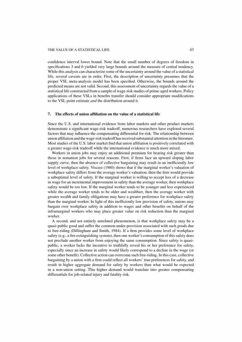
THE VALUE OF A STATISTICAL LIFE 43
confidence interval lower bound. Note that the small number of degrees of freedom inspecifications 3 and 6 yielded very large bounds around the measure of central tendency.While this analysis can characterize some of the uncertainty around the value of a statisticallife, several caveats are in order. First, the description of uncertainty presumes that theproper VSL meta-analysis model has been specified. Otherwise, the bounds around thepredicted means are not valid. Second, this assessment of uncertainty regards the value of astatistical life constructed from a sample of wage-risk studies of prime-aged workers. Policyapplications of these VSLs in benefits transfer should consider appropriate modificationsto the VSL point estimate and the distribution around it.
7. The effects of union affiliation on the value of a statistical life
Since the U.S. and international evidence from labor markets and other product marketsdemonstrate a significant wage-risk tradeoff, numerous researchers have explored severalfactors that may influence the compensating differential for risk. The relationship betweenunion affiliation and the wage-risk tradeoff has received substantial attention in the literature.Most studies of the U.S. labor market find that union affiliation is positively correlated witha greater wage-risk tradeoff while the international evidence is much more mixed.
Workers in union jobs may enjoy an additional premium for bearing risk greater thanthose in nonunion jobs for several reasons. First, if firms face an upward sloping laborsupply curve, then the absence of collective bargaining may result in an inefficiently lowlevel of workplace safety. Viscusi (1980) shows that if the marginal worker’s valuation ofworkplace safety differs from the average worker’s valuation, then the firm would providea suboptimal level of safety. If the marginal worker is willing to accept less of a decreasein wage for an incremental improvement in safety than the average worker, then workplacesafety would be too low. If the marginal worker tends to be younger and less experiencedwhile the average worker tends to be older and wealthier, then the average worker withgreater wealth and family obligations may have a greater preference for workplace safetythan the marginal worker. In light of this inefficiently low provision of safety, unions maybargain over workplace safety in addition to wages and other benefits on behalf of theinframarginal workers who may place greater value on risk reduction than the marginalworker.
A second, and not entirely unrelated phenomenon, is that workplace safety may be aquasi-public good and suffer the common under-provision associated with such goods dueto free-riding (Dillingham and Smith, 1984). If a firm provides some level of workplacesafety (e.g., a fire extinguishing system), then one worker’s consumption of this safety doesnot preclude another worker from enjoying the same consumption. Since safety is quasi-public, a worker lacks the incentive to truthfully reveal his or her preference for safety,especially since an increase in safety would likely correspond to a decline in the wage (orsome other benefit). Collective action can overcome such free-riding. In this case, collectivebargaining by a union with a firm could reflect all workers’ true preferences for safety, andresult in higher aggregate demand for safety by workers than what would be expectedin a non-union setting. This higher demand would translate into greater compensatingdifferentials for job-related injury and fatality risk.

44 VISCUSI AND ALDY
Third, if some workers lack adequate information about the safety at their workplace,then they may underestimate the actual risks they face. Workers underestimating their on-the-job risk would demand lower wages than if they held correct perceptions of risk. Unionspotentially could provide workers with more accurate information about their on-the-jobrisks (Viscusi, 1979; Olson, 1981). Unions can take advantage of economies of scale inproviding information not available to unorganized non-union workers (Dillingham andSmith, 1984). Unions may also negotiate for mechanisms that increase worker exposure tosafety information. For example, Olson noted that a 1976 BLS survey showed that 36 percentof all workers covered by a collective bargaining agreement worked in establishments thatsponsored joint firm-worker safety committees.
To evaluate the extent to which these factors influence compensating differentials foron-the-job risk, researchers have taken two estimation approaches (see Table 9). First, somehave split their samples into union and non-union subsamples and estimated the wageregressions separately for each subsample. Second, others have included an interactionterm, risk variable x union dummy variable, in the wage regression model. In our reviewof papers evaluating union effects, only Olson (1981) assessed the union-risk premiumwith both the separate sample regression approach and the risk-union interaction approach.Both approaches yield substantial differences in compensating differentials for union andnon-union members.
Regardless of estimation strategy, most assessments of the U.S. labor market found higherrisk premiums for union workers than for non-union workers (see Table 9(a)). Of the tenU.S. labor market value of life studies we reviewed that evaluated the role of unions in riskpremiums, nine found union workers enjoyed greater compensating differentials for bearingrisk than nonunion workers. In contrast to accepted theory, several of these papers foundthat non-union workers had insignificant or statistically significant negative compensatingdifferentials for risk.31
Table 9(b) summarizes the rather mixed effects of unionization on premiums for nonfatalrisks in the U.S. labor market. In the studies that controlled for fatal risks, the compensatingdifferential for injury risk for nonunion workers often exceeded the differential for unionworkers, even in the same studies where the union fatality risk premium was greater (e.g.,Olson, 1981; Dorsey, 1983; Dorsey and Walzer, 1984). Olson found that union workers en-joyed a greater positive premium than nonunion workers for injury incidence but a negativepremium for injury duration (number of lost workdays), in contrast to nonunion workers’positive premium.
In regressions that did not include a variable for fatality risk in the estimation model,the findings reflected the results for fatality risk discussed above. Hamermesh and Wolfe(1990) found that the extra compensating differential for union workers reflected injuryincidence, while injury duration was insignificant, similar to Olson. While Freeman andMedoff (1981) could not discern between the statistically significant injury risk premiumsfor union and non-union workers, Smith (1983), Biddle and Zarkin (1988), Fairris (1992),and Hersch and Pickton (1995) all found greater compensating differentials for nonfatalrisks for union than for nonunion workers.
While the majority of the U.S. research illustrates greater risk premiums for union work-ers, the research on labor markets in other countries often reveals a more ambiguous union
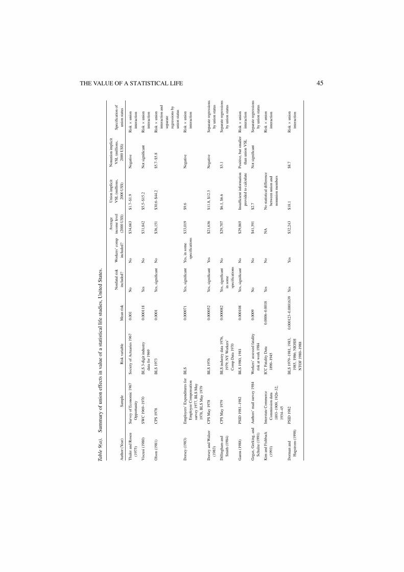
THE VALUE OF A STATISTICAL LIFE 45
Tabl
e9(
a).
Sum
mar
yof
unio
nef
fect
sin
valu
eof
ast
atis
tical
life
stud
ies,
Uni
ted
Stat
es.
Ave
rage
Uni
onim
plic
itN
onun
ion
impl
icit
Non
fata
lris
kW
orke
rs’
com
pin
com
ele
vel
VSL
(mill
ions
,V
SL(m
illio
ns,
Spec
ifica
tion
ofA
utho
r(Y
ear)
Sam
ple
Ris
kva
riab
leM
ean
risk
incl
uded
?in
clud
ed?
(200
0U
S$)
2000
US$
)20
00U
S$)
unio
nst
atus
Tha
ler
and
Ros
enSu
rvey
ofE
cono
mic
1967
Soci
ety
ofA
ctua
ries
1967
0.00
1N
oN
o$3
4,66
3$1
.7–$
1.9
Neg
ativ
eR
isk
×un
ion
(197
5)O
ppor
tuni
tyin
tera
ctio
n
Vis
cusi
(198
0)SW
C19
69–1
970
BL
S3-
digi
tind
ustr
y0.
0001
18Y
esN
o$3
1,84
2$5
.5–$
15.2
Not
sign
ifica
ntR
isk
×un
ion
data
for
1969
inte
ract
ion
Ols
on(1
981)
CPS
1978
BL
S19
730.
0001
Yes
,sig
nific
ant
No
$36,
151
$30.
6–$4
4.2
$5.7
–$5.
8R
isk
×un
ion
inte
ract
ion
and
sepa
rate
regr
essi
ons
byun
ion
stat
us
Dor
sey
(198
3)E
mpl
oyer
s’E
xpen
ditu
res
for
BL
S0.
0000
71Y
es,s
igni
fican
tY
es,i
nso
me
$33,
019
$9.6
Neg
ativ
eR
isk
×un
ion
Em
ploy
eeC
ompe
nsat
ion
spec
ifica
tions
inte
ract
ion
surv
ey19
77,B
LS
May
1978
,BL
SM
ay19
79
Dor
sey
and
Wal
zer
CPS
May
1978
BL
S19
760.
0000
52Y
es,s
igni
fican
tY
es$2
1,63
6$1
1.8,
$12.
3N
egat
ive
Sepa
rate
regr
essi
ons
(198
3)by
unio
nst
atus
Dill
ingh
aman
dC
PSM
ay19
79B
LS
indu
stry
data
1976
,0.
0000
82Y
es,s
igni
fican
tN
o$2
9,70
7$6
.1,$
6.6
$3.1
Sepa
rate
regr
essi
ons
Smith
(198
4)19
79;N
YW
orke
rs’
inso
me
byun
ion
stat
usC
omp
Dat
a19
70sp
ecifi
catio
ns
Gar
en(1
988)
PSID
1981
–198
2B
LS
1980
,198
10.
0001
08Y
es,s
igni
fican
tN
o$2
9,86
5In
suffi
cien
tinf
orm
atio
nPo
sitiv
e,bu
tsm
alle
rR
isk
×un
ion
prov
ided
toca
lcul
ate
than
unio
nV
SLin
tera
ctio
n
Geg
ax,G
erki
ng,a
ndA
utho
rs’
mai
lsur
vey
1984
Wor
kers
’as
sess
edfa
talit
y0.
0009
No
No
$41,
391
$2.7
Not
sign
ifica
ntSe
para
tere
gres
sion
sSc
hulz
e(1
991)
risk
atw
ork
1984
byun
ion
stat
us
Kim
and
Fish
back
Inte
rsta
teC
omm
erce
ICC
Fata
lity
Dat
a0.
0006
–0.0
018
Yes
No
NA
No
stat
istic
aldi
ffer
ence
Ris
k×
unio
n(1
993)
Com
mis
sion
data
1890
–194
5be
twee
nun
ion
and
inte
ract
ion
1893
–190
9,19
26–3
2,no
nuni
onm
embe
rs19
34–4
5
Dor
man
and
PSID
1982
BL
S19
79–1
981,
1983
,0.
0001
23–0
.000
1639
Yes
Yes
$32,
243
$18.
1$8
.7R
isk
×un
ion
Hag
stro
m(1
998)
1985
,198
6;N
IOSH
inte
ract
ion
NT
OF
1980
–198
8

46 VISCUSI AND ALDYTa
ble
9(b)
.Su
mm
ary
ofun
ion
effe
cts
inva
lue
ofst
atis
tical
inju
ryst
udie
s,U
nite
dSt
ates
.
Non
unio
nU
nion
impl
icit
impl
icit
valu
eW
orke
rs’
Ave
rage
valu
eof
ast
atis
tical
ofa
Fata
lris
kco
mp
inco
me
leve
lin
jury
stat
istic
alin
jury
Spec
ifica
tion
Aut
hor(
Yea
r)Sa
mpl
eR
isk
vari
able
Mea
nri
skin
clud
ed?
incl
uded
?(2
000
US$
)(2
000
US$
)(2
000
US$
)of
unio
nst
atus
Bid
dle
and
Zar
kin
(198
8)
QE
S19
77B
LS
nonf
atal
lost
wor
kday
inju
ryin
cide
ntra
te,
1977
0.03
7N
oN
o$4
2,17
0$3
19,6
78$5
6,83
2R
isk
×un
ion
inte
ract
ion
Free
man
and
Med
off
(198
1)
CPS
May
1973
–197
5B
LS
mea
nlo
stw
orkd
ays
per
wor
ker
1972
–197
4
0.70
1∗N
oN
oN
AN
ost
atis
tical
diff
eren
cebe
twee
nun
ion
and
nonu
nion
mem
bers
Sepa
rate
regr
essi
ons
byun
ion
stat
us
Smith
(198
3)C
PS19
78B
LS
wor
kin
jury
rate
0.07
8N
oN
o$3
8,13
8(m
ales
);$2
5,67
2(f
emal
es)
$74,
368
(mal
es);
$59,
815
(fem
ales
)
$46,
528
(mal
es);
$25,
672
(fem
ales
)
Ris
k×
unio
nin
tera
ctio
n
Fair
ris
(199
2)SW
C 1969
–197
0B
LS
1969
indu
stry
inju
ryfr
eque
ncy
rate
0.03
2N
oN
o$3
3,85
0$2
46,4
49N
otsi
gnifi
cant
Sepa
rate
regr
essi
ons
byun
ion
stat
us
Ham
erm
esh
and
Wol
fe(1
990)
PSID
1981
BL
S19
80,1
981
Inci
denc
e:0.
0476
;D
urat
ion:
0.15
71
No
Yes
NA
Insu
ffici
ent
info
rmat
ion
prov
ided
toca
lcul
ate
Posi
tive,
but
smal
ler
than
unio
nva
lue
ofin
jury
Ris
k×
unio
nin
tera
ctio
n
Her
sch
and
Pick
ton
(199
5)
Nat
iona
lM
edic
alE
xpen
ditu
reSu
rvey
1987
BL
Sto
tall
ost
wor
kday
spe
rw
orke
rpe
rye
ar19
87
0.70
2∗N
oN
o$2
6,34
5$2
22,4
48$9
9,47
8R
isk
×un
ion
inte
ract
ion
∗ Los
twor
kday
spe
r10
0fu
ll-tim
ew
orke
rs.

THE VALUE OF A STATISTICAL LIFE 47
Tabl
e9(
c).
Sum
mar
yof
unio
nef
fect
sin
valu
eof
ast
atis
tical
life
stud
ies,
inte
rnat
iona
l.
Uni
onN
onun
ion
Non
fata
lW
orke
rs’
Ave
rage
impl
icit
VSL
impl
icit
VSL
risk
com
pin
com
ele
vel
(mill
ions
,(m
illio
ns,
Spec
ifica
tion
Aut
hor
(Yea
r)C
ount
rySa
mpl
eR
isk
vari
able
Mea
nri
skin
clud
ed?
incl
uded
?(2
000
US$
)20
00U
S$)
2000
US$
)of
unio
nst
atus
Mar
inan
dPs
acha
ropo
ulos
(198
2)
UK
Gen
eral
Hou
seho
ldSu
rvey
1975
OPC
SO
ccup
atio
nal
Mor
talit
yD
ecen
nial
Surv
ey19
70–7
2
0.00
01N
oN
o$1
4,47
2N
ost
atis
tical
diff
eren
cebe
twee
nun
ion
and
nonu
nion
mem
bers
Ris
k×
unio
nin
tera
ctio
n
Men
g(1
989)
Can
ada
Nat
iona
lSur
vey
ofC
lass
Stru
ctur
ean
dL
abou
rPr
oces
s19
81
Lab
our
Can
ada
and
Que
bec
Occ
upat
iona
lH
ealth
and
Safe
tyB
oard
1981
0.00
019
No
No
$43,
840
No
stat
istic
aldi
ffer
ence
betw
een
unio
nan
dno
nuni
onm
embe
rs
Ris
k×
unio
nin
tera
ctio
n
Men
gan
dSm
ith(1
990)
Can
ada
Nat
iona
lE
lect
ion
Stud
y19
84
Lab
our
Can
ada
and
Que
bec
Occ
upat
iona
lH
ealth
and
Safe
tyB
oard
1981
–83
0.00
012
No
No
$29,
646
No
stat
istic
aldi
ffer
ence
betw
een
unio
nan
dno
nuni
onm
embe
rs
Ris
k×
unio
nin
tera
ctio
n
Men
g(1
991)
Can
ada
Lab
our
Mar
ket
Act
ivity
Surv
ey19
86
Lab
our
Can
ada
and
Wor
kers
’C
ompe
nsat
ion
Boa
rds
0.00
023
for
acci
dent
s,0.
0001
2fo
rdi
seas
e
No
No
$25,
387
$1.9
$4.2
Ris
k×
unio
nin
tera
ctio
n
(Con
tinu
edon
next
page
.)
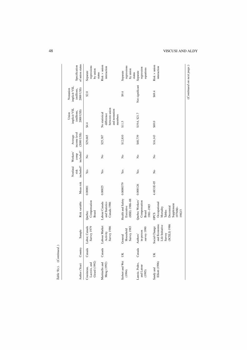
48 VISCUSI AND ALDY
Tabl
e9(
c).
(Con
tinu
ed.)
Uni
onN
onun
ion
Non
fata
lW
orke
rs’
Ave
rage
impl
icit
VSL
impl
icit
VSL
risk
com
pin
com
ele
vel
(mill
ions
,(m
illio
ns,
Spec
ifica
tion
Aut
hor
(Yea
r)C
ount
rySa
mpl
eR
isk
vari
able
Mea
nri
skin
clud
ed?
incl
uded
?(2
000
US$
)20
00U
S$)
2000
US$
)of
unio
nst
atus
Cou
sine
au,
Lac
roix
,and
Gir
ard
(199
2)
Can
ada
Lab
or,C
anad
aSu
rvey
1979
Que
bec
Com
pens
atio
nB
oard
0.00
001
Yes
No
$29,
665
$4.4
$2.0
Sepa
rate
regr
essi
ons
byun
ion
stat
usM
artin
ello
and
Men
g(1
992)
Can
ada
Lab
our
Mar
ket
Act
ivity
Surv
ey19
86
Lab
our
Can
ada
and
Stat
istic
sC
anad
a19
86
0.00
025
Yes
No
$25,
387
No
stat
istic
aldi
ffer
ence
betw
een
unio
nan
dno
nuni
onm
embe
rs
Ris
k×
unio
nin
tera
ctio
n
Sieb
erta
ndW
ei(1
994)
UK
Gen
eral
Hou
seho
ldSu
rvey
1983
Hea
lthan
dSa
fety
Exe
cutiv
e(H
SE)
1986
–88
0.00
0037
9Y
esN
o$1
2,81
0$1
1.5
$9.4
Sepa
rate
regr
essi
ons
byun
ion
stat
usL
anoi
e,Pe
dro,
and
Lat
our
(199
5)
Can
ada
Aut
hors
’in
-per
son
surv
ey19
90
Que
bec
Wor
kers
’C
ompe
nsat
ion
Boa
rd19
81–1
985
0.00
0126
Yes
No
$40,
739
$19.
6,$2
1.7
Not
sign
ifica
ntSe
para
tere
gres
sion
equa
tions
Sand
yan
dE
lliot
t(19
96)
UK
Soci
alC
hang
ean
dE
cono
mic
Lif
eIn
itiat
ive
Surv
ey(S
CE
LI)
1986
OPC
SO
ccup
atio
nal
Mor
talit
yTa
bles
Dec
enni
alSu
pple
men
t19
79/8
0–19
82/3
4.48
31E
-05
No
No
$16,
143
$69.
0$6
9.4
Ris
k×
unio
nin
tera
ctio
n
(Con
tinu
edon
next
page
.)

THE VALUE OF A STATISTICAL LIFE 49Ta
ble
9(c)
.(C
onti
nued
.)
Uni
onN
onun
ion
Non
fata
lW
orke
rs’
Ave
rage
impl
icit
VSL
impl
icit
VSL
risk
com
pin
com
ele
vel
(mill
ions
,(m
illio
ns,
Spec
ifica
tion
Aut
hor
(Yea
r)C
ount
rySa
mpl
eR
isk
vari
able
Mea
nri
skin
clud
ed?
incl
uded
?(2
000
US$
)20
00U
S$)
2000
US$
)of
unio
nst
atus
Shan
mug
am(1
996)
Indi
aA
utho
r’s
surv
eyof
blue
colla
rm
anuf
actu
ring
wor
kers
,M
adra
s,In
dia
1990
Adm
inis
trat
ive
Rep
orto
fFa
ctor
ies
Act
1987
–199
0
0.00
0104
No
No
$778
$0.6
Not
sign
ifica
ntR
isk
×un
ion
inte
ract
ion
Kim
and
Fish
back
(199
9)
Sout
hK
orea
Min
istr
yof
Lab
or’s
Rep
orto
nM
onth
lyL
abor
Surv
eyan
dSu
rvey
onB
asic
Stat
istic
sfo
rth
eW
age
Stru
ctur
es
Min
istr
yof
Lab
or’s
Ana
lysi
sfo
rIn
dust
rial
Acc
iden
ts
0.00
0485
Yes
Yes
$8,1
25N
ost
atis
tical
diff
eren
cebe
twee
nun
ion
and
nonu
nion
mem
bers
Ris
k×
unio
nin
tera
ctio
n
Ara
bshe
iban
ian
dM
arin
(200
0)
UK
Gen
eral
Hou
seho
ldSu
rvey
(198
0s)
OPC
SO
ccup
atio
nal
Mor
talit
yD
ecen
nial
Surv
ey19
79–8
3
Rep
orte
das
−0.0
06Y
esN
o$2
0,16
3N
ost
atis
tical
diff
eren
cebe
twee
nun
ion
and
nonu
nion
mem
bers
Ris
k×
unio
nin
tera
ctio
n
Bar
anzi
nian
dFe
rro
Luz
zi(2
001)
Switz
erla
ndSw
iss
Lab
our
Forc
eSu
rvey
,19
95,S
wis
sW
ages
Stru
ctur
eSu
rvey
,199
4
Swis
sN
atio
nal
Acc
iden
tIn
sura
nce
Com
pany
,19
91–1
995
0.00
0059
,0.
0000
64N
oN
o$4
7,40
0N
ost
atis
tical
diff
eren
cebe
twee
nun
ion
and
nonu
nion
mem
bers
Sepa
rate
regr
essi
ons
byun
ion
stat
us
Sand
yet
al.
(200
1)U
KSC
EL
I19
86O
PCS
79/8
0–82
/3,
HSE
1986
–88
0.00
0038
,0.
0000
45N
oN
o$1
6,14
3$5
.7,$
44.8
$36.
1,$7
4.1
Ris
k×
unio
nin
tera
ctio
n
50 VISCUSI AND ALDY
impact on risk premiums (Table 9(c)). Marin and Psacharopoulos (1982) conducted the firstanalysis of compensating differentials for risk in the U.K. labor market, and found that unionaffiliation had an insignificant impact on the risk premium. In an attempt to replicate thisinitial study, Arabsheibani and Marin (2000) also could not find any evidence supporting aunion-risk premium based on membership or union strength. In contrast, Siebert and Wei(1994) found higher union risk premiums when accounting for potential endogeneity ofrisk. Subsequent research by Sandy and Elliott (1996) countered this finding with analysisindicating larger compensating differentials for risk for nonunion members. These fourresearchers collaborated in a follow-up study, Sandy et al. (2001), which concluded with aqualified claim that nonunion workers enjoy greater risk premiums.
For the Canadian labor market, several analyses have found little support for a positiveimpact of union affiliation on compensating differentials for risk. In a series of analyses withunion x fatality risk interaction terms, Meng (1989, 1991) and Martinello and Meng (1992)found no significant effect for accident risk, while Meng and Smith (1990) found a negativestatistically significant coefficient that when combined with the fatality risk coefficientwould translate into no compensating differential for union members (in contrast to thepositive risk premium for non-union members). In contrast, Cousineau, Lacroix, and Girard(1992) found for a large Quebec sample that union members received larger premiums forboth fatality risk and injury incidence, but a smaller premium for injury duration, thannonunion members. Further, Lanoie, Pedro, and Latour (1995) found significant positivecompensating differentials for perceived risk for the union sub-sample from their survey ofMontreal work establishments.
Finally, the few analyses of developing country labor markets have also found mixedeffects of union affiliation on a worker’s risk premium. In his analysis of the Indian labormarket, Shanmugam (1996/7) included a union x fatality risk interaction term, and found thatunion members alone enjoy a compensating differential for risk. For the South Korean labormarket, Kim and Fishback (1999) could not statistically discern compensating differentialsfor risk between union and non-union workers.
8. The effects of age on the value of a statistical life
Evaluating wage-risk tradeoffs in labor markets to estimate the value of a statistical life raisesthe important question of whether life expectancy affects the value of a statistical life. Ageaffects the duration of life at risk and also may be correlated with other variables that affectone’s willingness to bear risk, which are not age effects per se but rather reflect changingpreferences over the life cycle. Numerous analyses have shown that the magnitude of theVSL is a decreasing function of age, whereas the value of any particular year of life mayincrease with age (Rosen, 1988).32 Wholly apart from life expectancy effects, accountingfor the effect of age in the utility function in terms of deteriorating health and quality of lifewould have generated similar results.33
Using this framework, Rosen undertook several simulations based on his previous em-pirical work (Thaler and Rosen, 1975). He estimated that the value of a statistical life-year,which is equal to the expected consumer surplus for another year, for the average-agedindividual in the sample ranges from about $31,000 to $130,000, based on discount rates
THE VALUE OF A STATISTICAL LIFE 51
ranging from 0 to 12 percent. Using data on life expectancy by age, Rosen calculated thevalue of a statistical life for comparable individuals who varied from 36 years to 48 yearsof age. The 48-year old’s VSL is 10 percent less than the 36-year old’s VSL.
Several researchers have undertaken direct empirical estimates of the effect of age on thereturn to risk in hedonic labor market analysis. A simple approach to estimating the effectrequires interacting the mortality risk and age variables in the regression model. Whilesome researchers did not identify significant coefficients to this interaction (Meng andSmith, 1990; Shanmugam, 1996/7, 2001), several others found statistically significant andnegative estimates broadly consistent with the theory (see Table 10). Research by Thalerand Rosen (1975), Viscusi (1979), Arnould and Nichols (1983) and Moore and Viscusi(1988b) yielded the negative relationship between age and the return to risk. Within thecontext of a local housing market, Portney (1981) found that the value of a statistical lifebased on trading off mortality risk associated with local air pollution exposure and housingprices declines significantly with age: an individual under the age of 45 has a VSL 20 timesgreater than an individual over the age of 65.
Dillingham, Miller, and Levy (1996) employed a modified approach by focusing on thewillingness to pay to avoid a fully impaired worklife, where death is the extreme case ofimpairment. The authors construct a risk variable that reflects injury frequency, severity, andprobability of fatality. They assume that a worklife shortened by a fatal injury is equivalent toa worklife shortened by a permanently disabling injury. Their “value of remaining worklife”ranges from $3.1–$4.7 million for the whole sample, although it decreases with age. Forexample, they estimate that a 50-year old values remaining worklife at half the value heldby a 30-year old.
Some researchers have proposed a value per discounted expected life-year approach(Moore and Viscusi, 1988b). In lieu of a value of a statistical life, one could adjust theVSL measure for the life expectancy of individuals by essentially annuitizing the estimatedVSL. Based on actuarial tables, one could estimate the life expectancy for the average-agedindividual in a study and then develop estimates of the life-year value (either by assuming adiscount rate, or as in several studies, estimating a discount rate based on revealed preferenceprocedures—see below). Then this life-year could be applied to other situations where lifeexpectancy would differ from the average in the study in question. This approach providesan “age-adjusted” or “life expectancy-adjusted” VSL alternative to the standard VSL. Whilethe life-year approach does address the concern that values of a statistical life should varywith life expectancy, they assume that the marginal value of another year is constant acrossthe age spectrum and across time for a given individual.34
Accounting for the effects of age on the value of a statistical life through a life-yearapproach requires the discounting of future consumer surplus (since, on the margin, thecompensating differential should equal the present discounted value of a worker’s expectedconsumer surplus). A variety of papers have imputed workers’ or consumers’ implicit ratesof discount (Moore and Viscusi, 1988b, 1990a, 1990b, 1990c; Viscusi and Moore, 1989;Dreyfus and Viscusi, 1995).35 While the Moore and Viscusi (1988b) and Dreyfus andViscusi papers estimate implicit discount rates and marginal discounted life-years based onreduced form models, the other three papers develop structural models to estimate discountrates. Also note that all of these models are based on data from labor markets, except for

52 VISCUSI AND ALDYTa
ble
10.
Sum
mar
yof
age-
risk
inte
ract
ion
effe
cts
inva
lue
ofa
stat
istic
allif
est
udie
s.
Ave
rage
age
Aut
hor
(Yea
r)Sa
mpl
eof
sam
ple
Ris
kva
riab
leA
ge×
risk
vari
able
coef
ficie
nt
Tha
ler
and
Ros
en(1
975)
Surv
eyof
Eco
nom
icO
ppor
tuni
ty19
6741
.8So
ciet
yof
Act
uari
es19
67Si
gnifi
cant
(5%
),ne
gativ
e
Vis
cusi
(197
9)Su
rvey
ofW
orki
ngC
ondi
tions
,19
69–1
970
(SW
C)
39.7
BL
S19
69,s
ubje
ctiv
eri
skof
job
(SW
C)
Sign
ifica
nt(1
%),
nega
tive
Port
ney
(198
1)Pr
oper
tyva
lues
inA
llegh
eny
Cou
nty,
PA19
78N
AA
irpo
llutio
nan
nual
mor
talit
yra
teda
ta,E
PAV
SLby
age
fem
ales
(mal
es):
less
than
45:$
1.5
(1.0
)m
illio
n;45
–64:
$0.3
(0.1
2)m
illio
n;ov
er65
:$0.
05(0
.05)
mill
ion
Arn
ould
and
Nic
hols
(198
3)U
.S.C
ensu
s19
70N
ASo
ciet
yof
Act
uari
es19
67Si
gnifi
cant
(1%
),ne
gativ
e
Moo
rean
dV
iscu
si(1
988b
)Q
ES
1977
38.1
Exp
ecte
dlif
eye
ars
lost
(=B
LS
fata
lity
risk
×di
scou
nted
rem
aini
nglif
e)
Sign
ifica
nt(1
%),
posi
tive
(im
plie
sri
skpr
emiu
min
crea
ses
with
life
expe
ctan
cy,d
ecre
ases
with
age,
cete
ris
pari
bus)
Men
g(1
989)
Nat
iona
lSur
vey
ofC
lass
Stru
ctur
ean
dL
abou
rPr
oces
s19
81
39.9
Lab
our
Can
ada
and
Que
bec
Occ
upat
iona
lHea
lthan
dSa
fety
Boa
rd19
81
Sign
ifica
nt(1
0%),
nega
tive
Men
gan
dSm
ith(1
990)
Nat
iona
lEle
ctio
nSt
udy
1984
NA
Lab
our
Can
ada
and
Que
bec
Occ
upat
iona
lHea
lthan
dSa
fety
Boa
rd19
81–8
3
Insi
gnifi
cant
Dill
ingh
am,M
iller
,and
Lev
y(1
996)
QE
S19
7736
.5C
onst
ruct
edri
skm
easu
reD
eclin
ing
scal
eof
WT
Pto
avoi
dim
pair
edw
orkl
ife
asfu
nctio
nof
age
Shan
mug
am(1
996/
7)A
utho
r’s
surv
eyof
blue
colla
rm
anuf
actu
ring
wor
kers
,M
adra
s,In
dia
1990
34.1
Adm
inis
trat
ive
Rep
orto
fFa
ctor
ies
Act
1987
–199
0In
sign
ifica
nt
Bar
anzi
nian
dFe
rro
Luz
zi(2
001)
Swis
sL
abou
rFo
rce
Surv
ey,
1995
,Sw
iss
Wag
esSt
ruct
ure
Surv
ey,1
994
NA
Swis
sN
atio
nalA
ccid
ent
Insu
ranc
eC
ompa
ny,
1991
–199
5
Sign
ifica
nt(1
%),
nega
tive
Shan
mug
am(2
001)
Aut
hor’
ssu
rvey
ofbl
ueco
llar
man
ufac
turi
ngw
orke
rs,
Mad
ras,
Indi
a19
90
34.1
Adm
inis
trat
ive
Rep
orto
fFa
ctor
ies
Act
1987
–199
0In
sign
ifica
nt

THE VALUE OF A STATISTICAL LIFE 53
Table 11. Summary of imputed discount rate studies, United States.
Implicitdiscount
Year Author (Year) Type of study Sample rate (%)
1988 Moore and Viscusi (1988b) Labor hedonic with reduced QES 1977 9.6–12.2form discounting model
1989 Viscusi and Moore (1989) Labor hedonic with structural PSID 1982 10.7Markov model
1990 Moore and Viscusi (1990b) Labor hedonic with structural PSID 1982 2.0life cycle model
1990 Moore and Viscusi (1990c) Labor hedonic with structural PSID 1982 1.0–14.2integrated life cycle model
1995 Dreyfus and Viscusi (1995) Automobile hedonic 1988 Residential 11–17Transportation EnergyConsumption Survey
the Dreyfus and Viscusi’s automobile hedonic study. Rational individuals can implicitlydiscount their health capital at a different rate than what they face in markets (e.g., realinterest rate for a home mortgage) since health status is a non-traded commodity (onecannot “save” good health at age 25 for consumption at age 75). Despite this possibility,these models estimate discount rates that are broadly consistent with the real rates of interesttypical workers and consumers face (see Table 11).
9. The application of the value of a statistical life to public policy decisions
At least in the countries with a high level of development, governments recommend or re-quire economic analyses of proposed regulations and public policies.36 Regulatory agenciesin the United States, the United Kingdom, and Canada, have been most prominent in theiruse of VSL estimates to value the benefits of proposed environmental, health, and safetyrules. In some cases, regulatory agencies have modified the VSL to account for distinctivecharacteristics of the risk and the affected population. In the United States, some environ-mental laws preclude the promulgation of regulations based on benefit-cost analysis. Inthese cases, analysts have turned to risk-risk analysis—based in part on an application ofthe value of a statistical life—to provide some guidance about whether a proposed policyis in fact risk reducing.
9.1. The use of VSLs in government decision-making around the world
9.1.1. United States. Over the past twenty years in the United States, executive orders byPresidents Carter, Reagan, and Clinton have mandated economic impact analyses of all sig-nificant Federal regulations (E.O. 12044, E.O. 12291 and E.O. 12866). Beginning with theReagan Administration, these executive orders vested with the Office of Management and

54 VISCUSI AND ALDY
Budget (OMB) the responsibility for overseeing and coordinating the review of regulatoryimpact analyses. OMB has published guidelines for all Federal agencies, such as its reportwith respect to the use of “best practices” in these analyses (U.S. OMB, 1996). The guid-ance recommends the use of a value of a statistical life to monetize the benefits associatedwith rules that change the population’s mortality risk. While OMB does not recommenda specific VSL or set of VSLs, it does provide a discussion of the issues agencies shouldconsider when choosing a VSL based on the current state of knowledge.
Until the 1980s the dominant policy approach to valuing the benefits of reduced risksof death was based on various human capital measures, such as the present value of lostearnings and medical expenses. These values are lower than the VSL amounts. Typicalof this approach was the 1982 analysis by OSHA of its proposed hazard communicationregulation. OSHA valued lives saved based on the cost of death, which was the humancapital value, because in its view life was too sacred to value. After OMB rejected theregulation, claiming that the costs exceeded the benefits, OSHA appealed the decision tothen Vice-President Bush. W. Kip Viscusi was asked to settle the economic dispute betweenthe two agencies. By valuing life properly using a VSL, the estimated benefits exceededthe costs. The regulation was approved the day after his analysis reached the Reagan WhiteHouse.37 Thus, the historical impetus for the adoption of the VSL methodology was thatthese values boosted assessed benefits by roughly an order of magnitude, improving theattractiveness of agencies’ regulatory efforts.
The flexibility provided to U.S. agencies in choosing a VSL appropriate to the populationaffected by their specific rules has resulted in significant variations in the selected VSL bothacross agencies and through time (see Table 12 and Adler and Posner, 2000). In addition,some regulatory impact analyses have included a range of benefits reflecting differentassumptions about the VSL, often reflecting the age profile of the affected population byusing a VSL adjusted by the number of life-years saved (e.g., the FDA rule restricting tobaccosales to children, 61 FR 44396, and the EPA rule regulating the sulfur content of gasoline,65 FR 6698). The U.S. Environmental Protection Agency (EPA), responsible for more costlyFederal rule-makings than any other U.S. agency, has developed economic guidelines forits regulatory impact analyses (U.S. EPA 2000a). The EPA guidelines recommend a VSL of$6.2 million (2000 US$), reflecting the arithmetic mean of 26 studies reviewed in Viscusi(1992a).
In contrast, the U.S. Federal Aviation Administration (1998) recommends a value of astatistical life of $3 million in its 2002 economic analyses of regulations.38 This compar-atively low value of life may reflect in part an anchoring effect. The U.S. Department ofTransportation was a leader in valuing mortality risk reductions, but began doing so in anera in which the present value of lost earnings was the dominant approach. The agency hasslowly increased the value attached to reduced risks of death, but it has continued to lagbehind the estimates in the literature.39
9.1.2. United Kingdom. In the United Kingdom, the Cabinet Office has likewise pro-vided guidance for economic analyses for the government’s regulatory and policy-makingagencies (U.K. Cabinet Office, 2000; H.M. Treasury, 1997). While the guidance does notspecify the value of a statistical life to be used by agencies, it does recommend careful
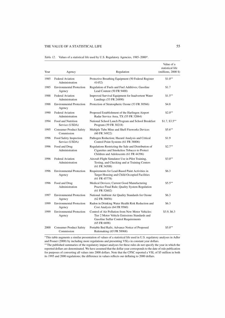
THE VALUE OF A STATISTICAL LIFE 55
Table 12. Values of a statistical life used by U.S. Regulatory Agencies, 1985–2000*.
Value of astatistical life
Year Agency Regulation (millions, 2000 $)
1985 Federal AviationAdministration
Protective Breathing Equipment (50 Federal Register41452)
$1.0∗∗
1985 Environmental ProtectionAgency
Regulation of Fuels and Fuel Additives; GasolineLead Content (50 FR 9400)
$1.7
1988 Federal AviationAdministration
Improved Survival Equipment for Inadvertent WaterLandings (53 FR 24890)
$1.5∗∗
1988 Environmental ProtectionAgency
Protection of Stratospheric Ozone (53 FR 30566) $4.8
1990 Federal AviationAdministration
Proposed Establishment of the Harlingen AirportRadar Service Area, TX (55 FR 32064)
$2.0∗∗
1994 Food and NutritionService (USDA)
National School Lunch Program and School BreakfastProgram (59 FR 30218)
$1.7, $3.5∗∗
1995 Consumer Product SafetyCommission
Multiple Tube Mine and Shell Fireworks Devices(60 FR 34922)
$5.6∗∗
1996 Food Safety InspectionService (USDA)
Pathogen Reduction; Hazard Analysis and CriticalControl Point Systems (61 FR 38806)
$1.9
1996 Food and DrugAdministration
Regulations Restricting the Sale and Distribution ofCigarettes and Smokeless Tobacco to ProtectChildren and Adolescents (61 FR 44396)
$2.7∗∗
1996 Federal AviationAdministration
Aircraft Flight Simulator Use in Pilot Training,Testing, and Checking and at Training Centers(61 FR 34508)
$3.0∗∗
1996 Environmental ProtectionAgency
Requirements for Lead-Based Paint Activities inTarget Housing and Child-Occupied Facilities(61 FR 45778)
$6.3
1996 Food and DrugAdministration
Medical Devices; Current Good ManufacturingPractice Final Rule; Quality System Regulation(61 FR 52602)
$5.5∗∗
1997 Environmental ProtectionAgency
National Ambient Air Quality Standards for Ozone(62 FR 38856)
$6.3
1999 Environmental ProtectionAgency
Radon in Drinking Water Health Risk Reduction andCost Analysis (64 FR 9560)
$6.3
1999 Environmental ProtectionAgency
Control of Air Pollution from New Motor Vehicles:Tier 2 Motor Vehicle Emissions Standards andGasoline Sulfur Control Requirements(65 FR 6698)
$3.9, $6.3
2000 Consumer Product SafetyCommission
Portable Bed Rails; Advance Notice of ProposedRulemaking (65 FR 58968)
$5.0∗∗
∗This table augments a similar presentation of values of a statistical life used in U.S. regulatory analyses in Adlerand Posner (2000) by including more regulations and presenting VSLs in constant year dollars.∗∗The published summaries of the regulatory impact analyses for these rules do not specify the year in which thereported dollars are denominated. We have assumed that the dollar year corresponds to the date of rule publicationfor purposes of converting all values into 2000 dollars. Note that the CPSC reported a VSL of $5 million in bothits 1995 and 2000 regulations; the difference in values reflects our deflating to 2000 dollars.
56 VISCUSI AND ALDY
consideration of the challenges in applying values estimated in the economic literature topotentially different risk and population contexts of the policy or regulation.
The U.K. Department of the Environment, Transport, and Regions (DETR; formerlyDepartment of Transport) has employed a willingness-to-pay based value of preventing afatality since 1988 in its regulatory and policy analyses (Chilton et al., 1999). The value ofpreventing a fatality selected in 1988, $1.2 million (£500,000 in 1987 prices), is still usedby the Department. This value reflects contingent valuation-based estimates of individuals’willingness-to-pay for risk reduction. The U.K. Health and Safety Executive uses the DETRvalue of preventing a fatality as a starting point for its regulatory impact analyses. The HSEhas employed a value of preventing a fatality double the DETR value for cancer-relatedfatalities, concluding that individuals’ dread of the disease significantly outweighs the affectsof latency on willingness-to-pay (Andrews and McCrea, 1999).40
Whereas U.S. agencies rely on market-based VSL estimates, in the U.K. the emphasisis on contingent valuation estimates. This difference in approach no doubt stems in partfrom the different character of the empirical evidence in the two countries. There have beendozens of studies of U.S. wage-risk tradeoffs, most of which have been in a reasonablerange. There have been far fewer such analyses for the U.K., and the resulting empiricalestimates have been much more unstable.
9.1.3. Canada. In Canada, the Privy Council Office published guidelines for benefit-costanalysis in 1995. While these guidelines do not specify one or a set of values of a statisticallife, they do note the need for serious consideration of the value of life, determinants of theappropriate VSL, and possible approaches to presenting useful information for policymakersand the public. The value of a statistical life is left to the discretion of agencies promulgatingregulations, again much like the U.S. and U.K. approaches.
Transport Canada reviewed the economic analyses for 145 transportation-related projectsover 1982–1993 (Blanchard, 1996). The VSL used in these analyses ranged from $400,000to $3.2 million. A recent analysis of a Canadian proposed rule on tobacco products informa-tion used a range of the value of a statistical life of $1.7–$5.7 million,41 with higher valuesfor individuals under age 65 (Hara Associates, 2000). A comparable range and age-basedVSL differential was employed in an evaluation of a Canadian proposal for cleaner fuels invehicles as well (Lang et al., 1995).
9.1.4. Multinational organizations. The value of a statistical life has also received atten-tion in multinational contexts. The Intergovernmental Panel on Climate Change (IPCC),established by the United Nations Environment Programme and the World Health Or-ganization in 1988 to provide technical support to participants in global climate changenegotiations, discussed issues regarding the value of a statistical life in its 1995 and 2001assessments of the economic and social dimensions of climate change (IPCC, 1996, 2001).Moreover, the European Commission (EC) began in 2000 a process to prepare guidancefor benefits analysis to improve benefit-cost analysis procedures within the EC. The ECeffort has focused a substantial amount of time and resources on the value of a statisticallife question (EC, 2000).
THE VALUE OF A STATISTICAL LIFE 57
9.2. Issues pertaining to benefits transfers
The vast majority of the studies reviewed in this paper cover prime-aged workers who havechosen to bear the risk of accidental, immediate death. Many of the studies based theirquantitative analyses on samples from the 1970s and 1980s. With the exception of occu-pational safety policies, most government regulations affect mortality risks with differentqualitative characteristics or affect populations with characteristics that differ from thoseof the samples in these studies. The demographic characteristics of specific groups and thepopulation at large likely differ today (and will differ in the future) from what they were20 to 30 years ago. The risk-money tradeoffs of those affected by government policy maydiffer from those values estimated in hedonic market studies.
For example, many environmental regulations address carcinogen exposure. Reducedcancer-related mortality presents several issues that merit consideration when employing aVSL. First, individuals may be willing to pay more to avoid dying of cancer than to avoid aninstantaneous accidental death. Revesz (1999) hypothesizes that this “dread” effect of cancermortality should result in an upward revision to the VSL. This reasoning apparently under-lies the higher VSL used by the UK Health and Safety Executive for cancer-related fatalities.The EPA’s Science Advisory Board (2000) recommended against any “dread”-related mod-ification to the value of a statistical life on the grounds that the current literature did notsupport any such change.42 In particular, contingent valuation estimates of cancer mortalityrisks have produced values similar to those observed for accidental deaths.43 The market-based evidence for cancer risks discussed above is similar to the results for accident risks.
Cancer-related mortality also differs significantly from occupational mortality in termsof the timing of the death. The long latency period for cancer (and other chronic healthconditions affected by government regulations) should be discounted in the benefits analysis(Revesz, 1999; Science Advisory Board, 2000). Given the rough similarity of the implicitrates of discount discussed in Section 8 to current market interest rates, a benefit-costanalysis could employ one common discount rate for all categories of benefits and costs.
Several researchers have questioned the discounting of benefits of reducing future risksto life when evaluating public policies. Heinzerling (1998, 1999, 2000) has criticized thediscounting of statistical lives on moral grounds. She claims that a statistical life cannotbe discerned from an actual life, which society would not attempt to price. This concernpertains to both current and future risk reductions and is not a discounting argument per se.While Heinzerling expresses significant concerns with the concept of statistical lives and intheir discounting, individuals make private risk-income, risk-time, and risk-risk tradeoffsevery day, as evidenced by the literature surveyed in this paper, as well as by simple casualobservation.44 Further, as the studies presented in Table 11 illustrate, individuals value risksin the future less than they value commensurate risks they face today. Both Revesz andHeinzerling raise concerns about discounting statistical lives in future generations (also seeArrow et al., 1996 for a survey of intergenerational discounting).
Failure to discount creates potentially fundamental paradoxes (see Keeler and Cretin,1983). Suppose that the cost structure for reducing risks to life is unchanged over time.Then it is always desirable to defer any life saving policy and invest the money that wouldhave been spent on risk reduction. Indeed, continual postponement of a life saving effort

58 VISCUSI AND ALDY
is always desirable if future benefits are never discounted, but the money spent on thesepolicies continues to grow at the rate of interest.
Similarly, suppose that future life saving benefits are not discounted. If, however, oneconverts the cost allocations to a terminal value rather than discounting the benefits back to apresent value, the effect will be identical in terms of whether the policy passes a benefit-costtest. What the discounting critics generally fail to grasp is that what is being discounted arenot lives but rather society’s willingness to pay for these future risks to life.
The differences in the age of the population in labor market studies and of the populationaffected by a regulation should also affect the value of a statistical life. While fewer studieshave focused on the effects of age on the return to risk, those that have tend to find thatthe value of a statistical life declines with age, consistent with the theoretical work. Sincethese labor hedonic studies include samples where age usually ranges no higher than about60 years, it may be difficult to extrapolate these results for older populations. This is asignificant issue in benefits transfer, since many environment and public health policies (asopposed to worker safety programs) deliver benefits to the elderly. For example, recent airquality regulations promulgated by the U.S. Environmental Protection Agency dispropor-tionately benefit older individuals as illustrated by the average increase in life expectancyof less than 15 years (U.S. EPA, 1999; Science Advisory Board, 1999a). In response tothis, the EPA’s Science Advisory Board (SAB) has questioned the appropriateness of EPA’schoice of a VSL for this population. The SAB notes that it “question[s] the application ofa WTP estimate for prime-aged individuals to a population of older individuals and peoplewho are in poor health” (p. 6). The SAB (1999b) has recommended that the EPA revise itsVSL in light of this concern.
Several agencies already employ age-adjusted VSLs. As noted above, the economicanalysis of a Canadian tobacco regulation employed a smaller VSL for individuals olderthan 65. The U.S. Food and Drug Administration regularly employs the value of statisticallife-years, instead of VSLs, as a way to monetize the health benefits of their proposedrules. The U.S. Environmental Protection Agency has reluctantly conducted benefit-costanalyses with the value of statistical life-years approach. The clear findings in the theory andexisting empirical evidence support such age adjustments. Future empirical research shouldfurther refine age-specific estimates of the value of a statistical life for use in regulatoryanalyses.
9.3. The role of risk-risk analysis
While the value of a statistical life can be used to monetize the benefits for risk policyevaluation, most laws do not require that agencies undertake such balancing and some lawsin the United States actually preclude the consideration of benefit-cost analysis in settingstandards. For example, the courts have interpreted the Clean Air Act such that the U.S.Environmental Protection Agency cannot base ambient air quality standards on benefit-cost analysis or an assessment of the costs.45 Even if a benefit-cost test cannot be applied,policies that on balance harm individual health presumably should not be adopted. Severalforms of risk-risk analysis can account for these various risk effects of policies in an effortto ascertain whether risk regulations on balance are risk reducing. While risk-risk analysis

THE VALUE OF A STATISTICAL LIFE 59
cannot determine if a policy improves societal welfare, it can identify the policies that clearlydo not improve societal welfare because they result in a net increase in mortality risk.
Four types of risk-risk tradeoffs could influence the net effect of a policy or regulation ona population’s risk exposure. First, a policy may reduce risks of one type while increasingrisks of another type. For example, the U.S. Food and Drug Administration consideredbanning saccharin, the artificial sweetener, in response to an animal study finding that itmay be a potential human carcinogen. However, banning saccharin would likely increasethe risks associated with obesity. In this case, the U.S. Congress allowed the use of saccharinin foods subject to a warning label on products containing the sweetener (Viscusi, 1994b).
Second, policies to reduce risks may create incentives for individuals to undertake lessindividual effort to reduce their exposure to risks (moral hazard). These behavioral responseswill offset some of the risk reduction of the policy, and could potentially increase netrisks. For example, Peltzman (1975) described how drivers responded to mandated safetydevices in automobiles by changing their driving behavior. Drivers in “safer cars” drovemore recklessly than before. The empirical evidence showed that while the safety measuresreduced fatalities among automobile occupants, these gains have been offset at least in partby increases in pedestrian deaths and nonfatal accidents.
Third, risk-reduction policies may result in regulatory expenditures that directly increasefatalities. For example, policies to remove asbestos from buildings may increase asbestosexposure by workers and use of excavation equipment at Superfund hazardous waste sitesmay result in construction-related injuries and fatalities (Graham and Wiener, 1995). Viscusiand Zeckhauser (1994) illustrate through an input-output analysis the total direct and indirectinjury and fatality risks associated with expenditures by industry. Regulations that require areallocation of resources to industries with higher risks, for example towards construction tobuild new wastewater treatment facilities or to install pollution control technologies, wouldresult in an offsetting increase in mortality risk.
Fourth, the costs of risk-reduction policies decrease income available to finance otherhealth and safety expenditures. Wildavsky (1980, 1988) noted that the costs of risk-reductionpolicies reduce national income, some of which would otherwise be used to promote healthand safety. This argument focuses on the correlation between income and health, evidentin both international cross-sectional data and U.S. time-series data (Viscusi, 1983, 1994b;Graham, Chang, and Evans, 1992; Lutter and Morrall, 1994; see Smith, Epp, and Schwabe,1994 for a critique of the international evidence).46 These analyses illustrate that wealthiercountries have lower mortality rates associated with greater health and safety investments.Graham, Chang, and Evans (1992) extended the previous analyses on the mortality-incomerelationship by focusing on the effect of permanent income. They conclude that: “If gov-ernment regulation reduces the level (or the rate of growth) of permanent income, it is likelyto cause smaller health investments and an eventual decline in health status compared towhat would have occurred without the economic burdens of regulation” (p. 336).47
Keeney (1990, 1994, 1997) formalized Wildavsky’s proposition and found that someexpensive regulations aimed at reducing mortality risks actually increase mortality risksby reducing national income. Keeney’s model yields various estimates for the induced-expenditure associated with an additional fatality that depend on the distribution of the bur-den of the policy costs. Based on the mortality-income relationships estimated by Kitawaga
60 VISCUSI AND ALDY
and Hauser (1973) and Frerichs et al. (1984), Keeney estimates that between $13.6 millionand $15.2 million of expenditures would induce a fatality, assuming costs are borne pro-portional to income.48,49 This research inspired a legal opinion of an OSHA regulation inthe early 1990s.50 U.S. Federal Appeals Court Judge Steven F. Williams wrote that regu-lations that do not pass a risk-risk analysis would be counterproductive. The U.S. Officeof Management and Budget then suggested to OSHA that it consider risk-risk analysis inconducting its regulatory impact analyses.
While the research on the income-mortality relationship influenced several policy dis-cussions in the early 1990s in the United States, the results from these studies point to-wards a peculiar inconsistency. For the studies with expenditure-induced fatalities on theorder of $5 million per fatality, the expenditure associated with a loss of one life is onpar or perhaps below what individuals are willing to pay to reduce the risk of one fatal-ity in the population based on the labor market hedonic studies (Viscusi, 1994b). More-over, the mortality-income studies also suffer several other potential problems. Some ofthese do not appropriately account for the simultaneity in the data—higher incomes al-low individuals to invest more in health, but poor health often draws down an individ-ual’s income (Chapman and Hariharan, 1994).51 Some of these studies also may sufferfrom omitted variable bias resulting in misidentifying the relationship between income andhealth.
As an alternative to deriving the income-mortality relationship from aggregate data,Viscusi (1994a) illustrates how to generate an estimate for the expenditure-induced fatalityrate based on the value of a statistical life and the marginal propensity to spend on health.Viscusi shows that
marginal expenditure per statistical life lost = value of a statistical life
marginal propensity to spend on health.
This approach requires an estimate of the value of a statistical life and an estimate ofthe marginal propensity to spend on health. The literature surveyed in previous sectionsprovides estimates for the numerator. For the marginal propensity to spend on health,Viscusi estimated this based on an analysis of 24 OECD countries over the 1960–1989period and a time-series analysis for the United States over the same period (Viscusi, 1992b,1994a, 1994b). Over an array of specifications for both data sets, the marginal propensityto spend on health ranged from 0.08 to 0.12. This implies that for every dollar increase innational income, an additional 8 to 12 cents are spent on health care. Assuming a marginalpropensity to spend on health of 0.1 and a VSL of about $6 million, the marginal expenditureper statistical life lost would be about $60 million.52
Lutter, Morrall, and Viscusi (1999) extended Viscusi’s (1994a) model to account for theeffect of income to influence risky behaviors (such as smoking, drinking, and poor diet)as well as the consumption of health care. Their statistical analyses illustrate that higherincomes promote better health habits, including reduced excessive drinking and cigarettesmoking and increased exercise. Including the effects of income on risky health behaviorreduces the estimated marginal expenditure per statistical life lost from the Viscusi (1994a)by more than a factor of 3 to $17 million. Lutter et al. note that policies that increase nationalincome would reduce one fatality for every $17 million increase. The authors also note that
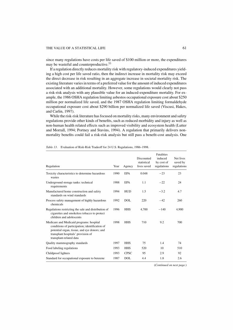
THE VALUE OF A STATISTICAL LIFE 61
since many regulations have costs per life saved of $100 million or more, the expendituresmay be wasteful and counterproductive.53
If a regulation directly reduces mortality risk with regulatory-induced expenditures yield-ing a high cost per life saved ratio, then the indirect increase in mortality risk may exceedthe direct decrease in risk resulting in an aggregate increase in societal mortality risk. Theexisting literature varies in terms of a preferred value for the amount of induced expendituresassociated with an additional mortality. However, some regulations would clearly not passa risk-risk analysis with any plausible value for an induced-expenditure mortality. For ex-ample, the 1986 OSHA regulation limiting asbestos occupational exposure cost about $250million per normalized life saved, and the 1987 OSHA regulation limiting formaldehydeoccupational exposure cost about $290 billion per normalized life saved (Viscusi, Hakes,and Carlin, 1997).
While the risk-risk literature has focused on mortality risks, many environment and safetyregulations provide other kinds of benefits, such as reduced morbidity and injury as well asnon-human health related effects such as improved visibility and ecosystem health (Lutterand Morrall, 1994; Portney and Stavins, 1994). A regulation that primarily delivers non-mortality benefits could fail a risk-risk analysis but still pass a benefit-cost analysis. One
Table 13. Evaluation of Risk-Risk Tradeoff for 24 U.S. Regulations, 1986–1998.
FatalitiesDiscounted induced Net livesstatistical by cost of saved by
Regulation Year Agency lives saved regulations regulations
Toxicity characteristics to determine hazardouswastes
1990 EPA 0.048 −23 23
Underground storage tanks: technicalrequirements
1988 EPA 1.1 −22 24
Manufactured home construction and safetystandards on wind standards
1994 HUD 1.5 −3.2 4.7
Process safety management of highly hazardouschemicals
1992 DOL 220 −42 260
Regulations restricting the sale and distribution ofcigarettes and smokeless tobacco to protectchildren and adolescents
1996 HHS 4,700 −140 4,900
Medicare and Medicaid programs: hospitalconditions of participation; identification ofpotential organ, tissue, and eye donors; andtransplant hospitals’ provision oftransplant-related data
1998 HHS 710 9.2 700
Quality mammography standards 1997 HHS 75 1.4 74
Food labeling regulations 1993 HHS 520 10 510
Childproof lighters 1993 CPSC 95 2.9 92
Standard for occupational exposure to benzene 1987 DOL 4.4 1.8 2.6
(Continued on next page.)

62 VISCUSI AND ALDY
Table 13. (Continued).
FatalitiesDiscounted induced Net livesstatistical by cost of saved by
Regulation Year Agency lives saved regulations regulations
Occupational exposure to methylene chloride 1997 DOL 12 5.9 6.2
Occupational exposure to 4,4′methylenedianiline
1992 DOL 0.7 0.71 −0.01
Asbestos: manufacture, importation, processing,and distribution in commerce—prohibitions(total)
1989 EPA 3.9 4.3 −0.41
National primary and secondary waterregulations–phase II: maximum contaminantlevels for 38 contaminants
1991 EPA 44 63 −19
Occupational exposure to asbestos 1994 DOL 13 20 −7.1
Hazardous waste management system—woodpreservatives
1990 EPA 0.29 0.83 −0.55
Sewage sludge use and disposal regulations,40 CFR pt. 503
1993 EPA 0.24 2.6 −2.3
Land disposal restrictions for “third third”scheduled wastes
1990 EPA 2.8 30 −27
Hazardous waste management system:final solvents and dioxins land disposalrestrictions rule
1986 EPA 1 12 −11
Occupational exposure to formaldehyde 1987 DOL 0.21 4.8 −4.5
Prohibit the land disposal of the first third ofscheduled wastes (“second sixth” proposal)
1988 EPA 2.9 66 −63
Land disposal restrictions—phase II: universaltreatment standards and treatment standardsfor organic toxicity, characteristic wastes,and newly listed wastes
1994 EPA 0.16 8.3 −8.2
Drinking water regulations, synthetic organicchemicals—phase V
1992 EPA 0.0061 3.4 −3.4
Solid waste disposal facility criteria, 40 CFR pt.257 and pt. 258
1991 EPA 0.0049 10 −10
Source: Hahn, Lutter, and Viscusi (2000).
approach could be to convert the morbidity effects into mortality risk equivalents. Alter-natively one could focus on policies whose primary intent is to reduce mortality risks.Recognizing this criticism, Hahn, Lutter, and Viscusi (2000) conducted risk-risk analyseson a number of major environment, health, and safety regulations over the 1986–1998 pe-riod whose primary benefits were reduced mortality risk (see Table 13).54 Their analysisfocuses on 24 regulations promulgated by the U.S. Environmental Protection Agency (EPA),U.S. Department of Housing and Urban Development (HUD), U.S. Department of La-bor (OSHA), and U.S. Consumer Products Safety Commission (CPSC). Thirteen of 24regulations designed primarily to reduce mortality risks actually increased mortality risks

THE VALUE OF A STATISTICAL LIFE 63
based on the Lutter et al. work finding that $15 million of expenditures induces a fatal-ity. Eight of these thirteen rules failing a risk-risk analysis had at least ten times moreexpenditure-induced fatalities than lives saved.55
10. Conclusion
For nearly thirty years, economists have attempted to infer individuals’ preferences overmortality and morbidity risk and income in labor and product markets. The substantialliterature that has developed over that time has confirmed Adam Smith’s intuition aboutcompensating differentials for occupational hazards in a significant and growing numberof countries. In addition to evaluating various international labor markets, the literature hasexpanded to address a variety of econometric issues, morbidity risk premiums, and factorsinfluencing mortality risk premiums such as union affiliation and age.
While the tradeoff estimates may vary significantly across studies, the value of a statisticallife for prime-aged workers has a median value of about $7 million in the United States. Ourmeta-analysis characterizes some of the uncertainty in estimates of the value of a statisticallife, and finds that the 95 percent confidence interval upper bounds can exceed the lowerbounds by a factor of two or more. Other developed countries appear to have comparableVSLs, although some studies of the United Kingdom have found much larger risk premiums.Consistent with the fact that safety is a normal good, developing countries’ labor marketsalso have significant, but smaller, values of statistical life. Overall, our point estimates ofthe income elasticity of the value of a statistical life range from 0.5 to 0.6. Union membersin U.S. labor markets appear to enjoy greater risk premiums than non-members, whilethe evidence in other developed countries is rather mixed. The theoretical and empiricalliterature indicates that the value of a statistical life decreases with age.
The estimates of the value of a statistical life can continue to serve as a critical input inbenefit-cost analyses of proposed regulations and policies. Refining VSLs for the specificcharacteristics of the affected population at risk remains an important priority for the researchcommunity and the government agencies conducting these economic analyses. Improvingthe application of VSLs in this way can result in more informed government interventionsto address market failures related to environmental, health, and safety mortality risks.
Appendix
Table A. Description of variables used in Viscusi-Aldy meta-analyses.
Summary statistic,Variable Description Viscusi-Aldy data
VSL Value of a statistical life (millions, 2000 US$) $6.7 ($5.6)
Income Annual labor income (2000 US$) $26,006 ($12,002)
Mean risk Average mortality risk of sample 0.0002 (0.0003)
Hourly wage Hourly wage or hourly equivalent of weekly income (2000 US$) $13.00 ($6.00)
Union VSL VSL for union members only (dummy variable) 4/49
(Continued on next page.)
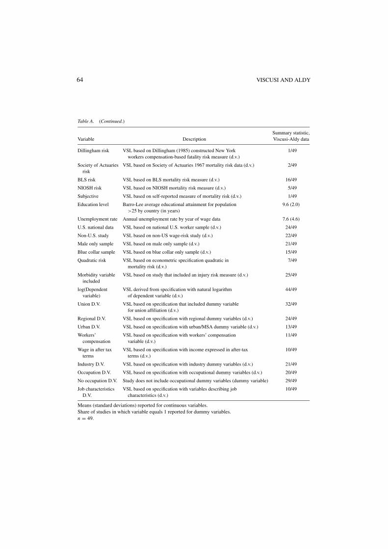
64 VISCUSI AND ALDY
Table A. (Continued.)
Summary statistic,Variable Description Viscusi-Aldy data
Dillingham risk VSL based on Dillingham (1985) constructed New York 1/49workers compensation-based fatality risk measure (d.v.)
Society of Actuaries VSL based on Society of Actuaries 1967 mortality risk data (d.v.) 2/49risk
BLS risk VSL based on BLS mortality risk measure (d.v.) 16/49
NIOSH risk VSL based on NIOSH mortality risk measure (d.v.) 5/49
Subjective VSL based on self-reported measure of mortality risk (d.v.) 1/49
Education level Barro-Lee average educational attainment for population 9.6 (2.0)>25 by country (in years)
Unemployment rate Annual unemployment rate by year of wage data 7.6 (4.6)
U.S. national data VSL based on national U.S. worker sample (d.v.) 24/49
Non-U.S. study VSL based on non-US wage-risk study (d.v.) 22/49
Male only sample VSL based on male only sample (d.v.) 21/49
Blue collar sample VSL based on blue collar only sample (d.v.) 15/49
Quadratic risk VSL based on econometric specification quadratic in 7/49mortality risk (d.v.)
Morbidity variable VSL based on study that included an injury risk measure (d.v.) 25/49included
log(Dependent VSL derived from specification with natural logarithm 44/49variable) of dependent variable (d.v.)
Union D.V. VSL based on specification that included dummy variable 32/49for union affiliation (d.v.)
Regional D.V. VSL based on specification with regional dummy variables (d.v.) 24/49
Urban D.V. VSL based on specification with urban/MSA dummy variable (d.v.) 13/49
Workers’ VSL based on specification with workers’ compensation 11/49compensation variable (d.v.)
Wage in after tax VSL based on specification with income expressed in after-tax 10/49terms terms (d.v.)
Industry D.V. VSL based on specification with industry dummy variables (d.v.) 21/49
Occupation D.V. VSL based on specification with occupational dummy variables (d.v.) 20/49
No occupation D.V. Study does not include occupational dummy variables (dummy variable) 29/49
Job characteristics VSL based on specification with variables describing job 10/49D.V. characteristics (d.v.)
Means (standard deviations) reported for continuous variables.Share of studies in which variable equals 1 reported for dummy variables.n = 49.

THE VALUE OF A STATISTICAL LIFE 65
Acknowledgments
Viscusi’s research is supported by the Harvard Olin Center for Law, Business, and Eco-nomics, and the Environmental Protection Agency. Aldy’s research is supported by theEnvironmental Protection Agency STAR Fellowship program. The authors thank JamesHammitt, Randall Lutter, and Robert S. Smith for helpful comments on an earlier draft ofthis paper.
Notes
1. Past reviews of this literature include Smith (1979), Miller (1990), and Viscusi (1992, 1993, 2000). Severalresearchers have conducted meta-analyses of this literature, including Liu, Hammitt, and Liu (1997), Miller(2000), Bowland and Beghin (2001), and Mrozek and Taylor (2002). See Hammitt (2002) and Krupnick(2002) for commentaries on the Mrozek and Taylor paper.
2. For more extensive discussion of hedonic analysis, see Griliches (1971), Rosen (1974, 1986), Thaler andRosen (1975), Smith (1979), and Viscusi (1979).
3. For a discussion of irrational behavior in the presence of mortality risk inconsistent with expected utilitytheory, refer to Viscusi (1998).
4. Individual risk neutrality or risk aversion, i.e., U ′′, V ′′ ≤ 0 is required to ensure a global maximum.5. Gaba and Viscusi (1998) compared qualitative and quantitative subjective measures of on-the-job accident
risk. They find that for a given level of quantitative risk, a college-educated individual is more likely toreport that risk as “dangerous” than an individual with less than college education. For example, for thoseworkers who report their quantitative risk as comparable to an annual injury risk of less than 1 in 20, half ofthe college-educated described their job risk as “dangerous” while only 19 percent of the less-than-collegeeducated reported their job risk as such. This differences in the “danger” cutoff biases estimates of riskpremiums in wages, and this bias has implications distinct from typical measurement error. Gaba and Viscusifind that subjective quantitative measures of risk yielded wage premiums more consistent with estimates basedon objective risk measures (BLS). Analysis of the qualitative risk measure (a dichotomous 0-1 “is the jobdangerous?” variable) produced a much larger risk premium.
6. Averaging over a period of 5 to 10 years would likely remove any potential distortions associated withcatastrophic accidents in any particular year.
7. Viscusi (1979, 1980) includes the danger variable in some regressions, although his research focused oncompensating differentials based on BLS measures of injury and fatality risk discussed below.
8. Leigh’s (1991) analysis with risk data derived from workers’ compensation records in 11 states appears to bethe only U.S. study to aggregate such data from more than one state.
9. Averaging fatality risk data over several years can reduce the distortion of a catastrophic event in one year inone industry on the measure of an industry’s risk.
10. Most hedonic wage-risk studies have not accounted for labor taxes in their construction of the wage variableor in their interpretation of the value of a statistical life. Exceptions include several papers that have focusedon the effects of workers’ compensation on the compensating differential for occupational risk (e.g., Mooreand Viscusi, 1990a). This reflects the more common use of pre-tax wages in the broader labor market analysisliterature.
11. In the product market context, Atkinson and Halvorsen (1990), Dreyfus and Viscusi (1995), and Gayer,Hamilton, and Viscusi (2000) employ Box-Cox transformations to evaluate their respective hedonic pricemodels (the first two focused on automobile prices and the third on housing prices).
12. Viscusi (1978a) excluded the dummy variables out of concern of inducing multicollinearity between anindustry-level risk measure and industry dummy variables. Refer to the discussion below on multicollinearity.
13. We focus our discussion here on their NIOSH data-based results for several reasons. First, we believe that theNIOSH data are superior to the 1980s BLS fatality risk data as discussed above. Second, the regression modelsbased on non-NIOSH data in Dorman and Hagstrom have insignificant risk coefficients for all specifications—without industry dummy variables, with industry dummy variables, and with other industry characteristics.
66 VISCUSI AND ALDY
While we are not certain why they did not find significant risk coefficients with the BLS risk data as previousresearchers had, it seems moot to argue that a coefficient on a risk variable actually represents an industryeffect if that coefficient is not significant.
14. We selected papers for inclusion in this literature review with a modest set of criteria. First, a study shouldbe written in English. Second, a study should be published in either an academic journal or a book. Third, astudy should provide enough information to calculate a value of a statistical life. In several cases, informationprovided in more recent papers (such as per capita incomes reported for some studies in Viscusi, 1993; Mrozekand Taylor, 2002) has been used with reported coefficient estimates to calculate the value of a statistical lifefor a study. Our aim is to characterize as best as possible the universe of wage-risk studies in the literature,so we have not attempted to purge this assessment of so-called “low quality” studies or to modify the valueof a statistical life estimates from such studies. For some studies, we have presented a range of the value ofa statistical life estimates and for others we have presented an illustrative point estimate. In the case of thelatter, we have focused on the reported results for the whole sample (as opposed to union-only, blue-collaronly, managerial-only, etc. samples) based on the econometric specification preferred by the studies’ authors.
15. While these estimates have been adjusted to constant year dollars (2000 US$), they have not been adjustedfor differences in the samples’ income levels. The per capita income data provided in Table 2 coupled withincome elasticity estimates in Section 6 can be used to modify the values of a statistical life in Table 2 so thatthey reflect a common income level.
16. In this paper, we present all VSLs in terms of 2000 US$. All domestic values are converted using the CPI-Udeflator series (Council of Economic Advisers, 2002, Table B60). International conversions are made usingpurchasing power parity exchange rates from the Penn World Table 6.0 (see Summers and Heston, 1991; Atenet al., 2001, and Internet: http://pwt.econ.upenn.edu) and then converted to year 2000 dollars with the CPI-Udeflator series.
17. Viscusi (1993) actually reports $3–$7 million in December 1990 US$. This has served as a reference rangein several subsequent value of a statistical life studies. Note that we have updated this range to 2000 US$.
18. Also refer to Fishback and Kantor (1992) for a historical evaluation of compensating differentials for occu-pational risk in the late 19th century.
19. Smith (1983) also used the Hickey and Kearney carcinogen exposure index to complement his assessmentof compensating differentials for injury risk in U.S. labor markets. He found that the index is significantlypositively correlated with wages implying a risk premium for workers’ operating in environments exposingthem to more carcinogens. Further, Smith included a measure of total suspended particulates (TSP) based onthe workers’ locations and found a statistically significant and positive correlation between TSP and workers’wages. Since TSP has been linked with various respiratory diseases, this could illustrate another premium forworkers’ bearing long-term risks on the job.
20. The values we report reflect an assumed latency period of 10 years and a real discount rate of 3 percent.Note that the VSL estimates in parentheses in Table 2 represent the values reported by Lott and Manning.Employing a real discount rate of 7 percent, consistent with U.S. Office of Management and Budget (1992)guidance, over a 10-year period effectively reduces the VSL reported by Lott and Manning in half.
21. Meng (1991) attempted to account for occupational disease by including a variable that reflected the rateof heart attacks and industrial disease. However, very modest information about the basis for this variableis provided. It is difficult to discern whether the variable captures long-term work-related risks or simply aselection effect that contaminates the data like the Society of Actuaries data set.
22. The authors also report estimates using the less reliable pre-1992 BLS risk data.23. Siebert and Wei (1998) found a concave wage-risk relationship with a risk and risk-squared specification for
their analysis of the Hong Kong labor market. Meng and Smith (1990, 1999) found the same relationship intheir assessments of the Canadian labor market. Baranzini and Ferro Luzzi (2001) likewise found the samerelationship in their analysis of the Swiss labor market.
24. All these studies evaluate risk-income tradeoffs in the United States. In our survey of the literature, we foundonly one study focusing on behavior outside of the United States. Ghosh, Lees, and Seal (1975) study thetradeoff between highway speeds and mortality risk in the United Kingdom. They derive a value of a statisticallife estimate of $0.9 million.
25. We have discounted the reported VSLs assuming that homeowners perceive a 10-year latency period and usea 3 percent discount rate in making their housing decisions.

THE VALUE OF A STATISTICAL LIFE 67
26. The difference between the mean subjective mortality risk and the objective mortality risk reported by theTaiwan Labor Insurance Agency is statistically significant at the 1 percent level.
27. Studies for which we do not have an income measure were omitted. We did not include the Baranzini andFerro Luzzi paper on the Swiss labor market since we became aware of it in the spring of 2003, well aftercompleting this analysis.
28. We also estimated a regression with the Mrozek and Taylor set of control variables, with an importantexception of replacing the hourly earnings variable with the natural logarithm of annual income. With an OLSspecification, we estimated an income elasticity of 0.76 with a 95 percent confidence interval of 0.20–1.32(n = 41). In the robust regression with Huber weights specification, we estimated again a point estimate forthe income elasticity of 0.76, but with a much tighter 95 percent confidence interval of 0.73–0.79 (n = 38).The income variable was statistically significant at the 5 percent level in the OLS regression and significantat the 1 percent level in the robust regression. The iterative weighting process in robust regression with thismuch larger set of control variables effectively eliminated several low-VSL studies relative to specification 6in Table 8, which may have resulted in the larger elasticity.
29. The Science Advisory Board (2000) has supported EPA’s adjustment of the VSL for income growth.30. We also calculated the median predicted VSL values for the full and U.S. samples. For the full sample,
the median predicted VSL never exceeded the mean predicted VSL in any of the six regression models bymore than 14 percent, and the mean predicted VSL never exceeded the median predicted VSL by more than15 percent. For the U.S. sample, the median predicted VSL exceeded the mean predicted VSL in all sixregressions, but never by more than 7 percent.
31. For example, Dorsey (1983) estimated a statistically significant negative coefficient on the fatality riskvariable and a statistically significant positive coefficient on the union x risk interaction variable. Thiscombination (with the union x risk coefficient greater in magnitude than the fatality risk coefficient) re-sults in a positive compensating differential for union workers and a negative differential for non-unionworkers.
32. Rosen’s research yields results similar to the Jones-Lee (1976), Jones-Lee, Hammerton, and Phillips (1985)and Shepard and Zeckhauser (1982, 1984) finding that the value of a statistical life takes an inverted-U shapewith respect to age. Also refer to Garber and Phelps (1997) for an assessment of quality-adjusted life-years(QALYs) in the cost-effectiveness literature. Jenkins, Owens, and Wiggins (2001) provide some evidence thatthe value of a statistical life is increasing over childhood through the pre-retirement years.
33. Modifying utility functions in this way would be analogous to constructing QALY measures, common tovaluations based on health status in the health economics literature. The QALYs are usually based on statedpreference methods (see Cutler and Richardson, 1997).
34. Based on Rosen’s life cycle model, one would expect that the marginal value of another year is greater for anelderly person than for a middle-aged person but that the value of all future years declines with age for a givenindividual. Accounting for health status may counter the effect of increasing marginal values for a one-yearlife extension for an elderly person. If health status is decreasing in age, then it may be ambiguous whetherthe marginal value of another year increases with age.
35. Baranzini and Ferro Luzzi (2001) also conducted such an analysis of the Swiss labor market with the samemethod as used by Moore and Viscusi (1988b). Consistent with the results for the U.S. labor market, theyfound that the value of a statistical life is increasing in life expectancy. In Switzerland, they estimate that a50-year old values his life less than one-half as much as a 35-year old.
36. For example, refer to the guidance to improve regulatory decision-making provided by the OECD (1995) toits member countries.
37. For a review of the substance of this analysis, see Viscusi (1992a).38. Refer to Table E-1 at Internet: http://www.api.faa.gov/economic/EXECSUMM.PDF and http://www.api.
faa.gov/economic/742SECT2.PDF.39. The low VSL used by the agency also reflects a political dimension as well. In the early 1990s when Viscusi
prepared the report that was subsequently published as Viscusi (1993) for the Federal Aviation Administration,that branch of the agency favored a higher value of life than was later mandated for use throughout thedepartment.
40. Note that the Science Advisory Board to the U.S. Environmental Protection Agency considered the effects oflatency and dread within the context of cancer-related mortality. The SAB (2000) concluded that the literature

68 VISCUSI AND ALDY
does not currently support a modification of the value of a statistical life to reflect dread. In contrast, the SABdid recommend that economic analyses account for latency by discounting future mortality to the present timeconsistent with the approach to other categories of benefits and costs.
41. The conversion to U.S. dollars for the Hara Associates analysis was based on the annual market exchangerate reported by the Federal Reserve (refer to Internet: http://www.federalreserve.gov/releases/g5a/current/)because the Penn World Table does not provide conversions for the most recent years.
42. While Revesz suggests other adjustments to the value of a statistical life based on the qualitative characteristicsof the risk, such as involuntariness of the risk, the Science Advisory Board (2000) noted that the existingliterature does not justify adjustments for these effects.
43. See Magat, Viscusi, and Huber (1996).44. This discussion implicitly acknowledges an important aspect of most occupational, safety, and environmental
health risks: these risks are relatively small. In cases of certain, or near-certain death, the empirical economicevidence and this argument are not relevant (see our discussion in Section 1).
45. For example, the 1997 final rule for the national ambient air quality standard for ozone introduced thesection on the regulatory impact analysis with the following: “As discussed in Unit IV of this preamble, theClean Air Act and judicial decisions make clear that the economic and technological feasibility of attainingambient standards are not to be considered in setting NAAQS, although such factors may be considered inthe development of State plans to implement the standards. Accordingly, although, as described below, aRegulatory Impact Analysis (RIA) has been prepared, neither the RIA nor the associated contractor reportshave been considered in issuing this final rule” (62 FR 38856).
46. This relationship is also revealed within a cross-section of the U.S. population. Viscusi (1978b) found thatwork-related risk exposure decreases with worker wealth.
47. Portney and Stavins (1994) question whether the income losses from regulations would reduce the population’shealth status. They claim that the nonlinear relationship between income and health and the modest impact ofmost regulations on the economy would not likely have a significant effect on health status. While individualregulations may involve small costs as a share of the economy, it is important to note that environmentalregulations alone cost about 1–2 percent of U.S. economic output (U.S. OMB, 2001).
48. We have updated the reported values in Keeney (1990) to 2000 U.S. dollars using the CPI-U deflator.49. The Keeney estimates are near the high end of 11 studies cited in Lutter and Morrall (1994) on the income
gains necessary to avert one fatality. They are very similar to Lutter and Morrall’s estimated range of $11.4million to $15.2 million for the United States.
50. Refer to UAW v. OSHA, United States Court of Appeals for the District of Columbia Circuit, 89-1559.51. A recent paper by Gerdtham and Johannesson (2002) attempts to address this problem by controlling for initial
health status in regressions of mortality risk on income (with other relevant controls) for a study focusingon Sweden in the 1980s and 1990s. They find that an income loss ranging from $7.5–$10.8 million wouldinduce an expected fatality in Sweden. The range reflects variation in the progressivity of the burden of theregulation.
52. Viscusi (1994a, 1994b) selected a VSL estimate of $5 million (in 1992 US$) because it represented themidpoint of the basic range for VSLs of $3 million–$7 million in Viscusi (1993). In 2000 US$, the midpointwould be $6.1 million.
53. Refer to Morrall (1986) and Tengs et al. (1995) for lists of regulations’ cost-effectiveness for the UnitedStates. Tengs et al. found that for 124 environmental regulations (primarily toxin control), the median cost perlife-year saved is $3.3 million. About 15 percent of the environmental regulations exceeded $100 million perlife-year saved. Converting these life-year values to statistical life values would result in a significant numberof regulations with incredibly exorbitant cost-effectiveness measures. Life-saving regulations in other sectorsof the economy (e.g., health care, transportation) had much lower costs per life-year saved. Refer to Ramsbergand Sjoberg (1997) for an evaluation of the cost-effectiveness of lifesaving interventions in Sweden.
54. Hahn, Lutter, and Viscusi only considered regulations with reduced mortality risk benefits comprising at least90 percent of total monetized benefits.
55. Note that the construction of discounted statistical lives saved reflects both an accounting for life-years savedand discounting for latency.
THE VALUE OF A STATISTICAL LIFE 69
References
Adler, M.D. and E.A. Posner. (2000). “Implementing Cost-Benefit Analysis When Preferences Are Distorted,”Journal of Legal Studies 29, 1105–1148.
Andrews, R.M. and P. McCrea. (1999). “UK Health and Safety Executive Approach to Exposure Limit Setting.”In Proceedings of the OECD Workshop on the Integration of Socio-Economic Analysis in Chemical RiskManagement Decision Making, London, January 7–9, 1998. Paris: Organization of Economic Cooperation andDevelopment, pp. 193–202.
Arabsheibani, G.R. and A. Marin. (2000). “Stability of Estimates of the Compensation for Danger,” Journal ofRisk and Uncertainty 20(3), 247–269.
Arnould, R.J. and L.M. Nichols. (1983). “Wage-Risk Premiums and Workers’ Compensation: A Refinement ofEstimates of Compensating Wage Differential,” Journal of Political Economy 91(2), 332–340.
Arrow, K.J., W.R. Cline, K.-G. Maler, M. Munasinghe, J.E. Stiglitz, and R. Squitieri. (1996). “IntertemporalEquity and Discounting.” In J.P. Bruce, H. Lee, and E. Haites (eds.), Climate Change 1995: Economic andSocial Dimensions. Cambridge, England: Cambridge University Press, pp. 125–144.
Aten, B., R. Summers, and A. Heston. (2001). The Penn World Table Mark 6. Philadelphia, PA: The Center forInternational Comparisons at the University of Pennsylvania. Internet: http://pwt.econ.upenn.edu.
Atkinson, S.E. and R. Halvorsen. (1990). “The Valuation of Risks to Life: Evidence from the Market for Auto-mobiles,” Review of Economics and Statistics 72(1), 133–136.
Baranzini, A. and G. Ferro Luzzi. (2001). “The Economic Value of Risks to Life: Evidence from the Swiss LabourMarket,” Swiss Journal of Economics and Statistics 137(2), 149–170.
Barro, R.J. and J.W. Lee. (1996). “International Measures of Schooling Years and Schooling Quality,” AmericanEconomic Review 86(2), 218–223.
Berger, M.C. and P.E. Gabriel. (1991). “Risk Aversion and the Earnings of U.S. Immigrants and Natives,” AppliedEconomics 23, 311–318.
Biddle, J.E. and G.A. Zarkin. (1988). “Worker Preference and Market Compensation for Job Risk,” Review ofEconomics and Statistics 70(4), 660–667.
Blanchard, G. (1996). Highway Benefit-Cost Analysis: A Review of Evidence. Transport Canada, Economic Anal-ysis, Special Infrastructure Project. Report no. TP12790E. Ottawa, Ontario.
Blomquist, G. (1979). “Value of Life Saving: Implications of Consumption Activity,” Journal of Political Economy87(3), 540–558.
Blomquist, G.C., T.R. Miller, and D.T. Levy. (1996). “Values of Risk Reduction Implied by Motorist Use ofProtection Equipment,” Journal of Transport Economics and Policy 30(1), 55–66.
Bowland, B.J. and J.C. Beghin. (2001). “Robust Estimates of Value of a Statistical Life for Developing Economies,”Journal of Policy Modeling 23, 385–396.
Brown, C. (1980). “Equalizing Differences in the Labor Market,” Quarterly Journal of Economics 94(1), 113–134.Bureau of Labor Statistics. (n.d.). Census of Fatal Occupational Injuries. Washington, DC: Department of Labor.
Internet: http://www.bls.gov/iif/oshcfoi1.htm.Butler, R.J. (1983). “Wage and Injury Rate Responses to Shifting Levels of Workers’ Compensation.” In J.D.
Worrall (ed.), Safety and the Workforce: Incentives and Disincentives in Workers’ Compensation. Ithaca, NY:ILR Press, pp. 61–86.
Carlin, P.S. and R. Sandy. (1991). “Estimating the Implicit Value of a Young Child’s Life,” Southern EconomicJournal 58(1), 186–202.
Chapman, K.S. and G. Hariharan. (1994). “Controlling for Causality in the Link from Income to Mortality,”Journal of Risk and Uncertainty 8(1), 85–94.
Chilton, S., J. Covey, L. Hopkins, M. Jones-Lee, G. Loomes, N. Pidgeon, and A. Spencer. (1999). “Annex:New Research Results on the Valuation of Preventing Fatal Road Accident Casualties.” In Health Costs Dueto Road Traffic-Related Air Pollution: Economic Evaluation, Prepared for the WHO Ministerial Conferenceon Environment and Health, London, June 1999. Bern, Switzerland: Federal Department of Environment,Transport, Energy and Communications, Bureau for Transport Statistics.
Council of Economic Advisers. (2002). Economic Report of the President. Washington, DC: Government PrintingOffice.
70 VISCUSI AND ALDY
Cousineau, J.-M., R. Lacroix, and A.-M. Girard. (1992). “Occupational Hazard and Wage Compensating Differ-entials,” Review of Economics and Statistics 74(1), 166–169.
Cutler, D.M. and E. Richardson. (1997). “Measuring the Health of the U.S. Population,” Brookings Papers onEconomic Activity, Microeconomics 1997, 217–271.
Dardis, R. (1980). “The Value of Life: New Evidence from the Marketplace,” American Economic Review 70(5),1077–1082.
Desvousges, W.H., F.R. Johnson, H.S. Banzhof, R.R. Russell, E.E. Fries, K.J. Dietz, and S.C. Helms. (1995).Assessing the Environmental Externality Costs for Electricity Generation. Research Triangle Park, NC: TriangleEconomic Research.
Dickens, W.T. (1984). “Differences Between Risk Premiums in Union and Nonunion Wages and the Case forOccupational Safety Regulation,” American Economic Review 74(2), 320–323.
Dillingham, A.E. (1985). “The Influence of Risk Variable Definition on Value-of-Life Estimates,” EconomicInquiry 23(2), 277–294.
Dillingham, A.E., T. Miller, and D.T. Levy. (1996). “A More General and Unified Measure for Valuing LabourMarket Risk,” Applied Economics 28, 537–542.
Dillingham, A.E. and R.S. Smith. (1984). “Union Effects on the Valuation of Fatal Risk.” In Dennis, B.O. (ed.), Pro-ceedings of the Industrial Relations Research Association 36th Annual Meeting. San Francisco, CA, December28–30, 1983. Madison, WI: Industrial Relations Research Association, pp. 270–277.
Dorman, P. and P. Hagstrom. (1998). “Wage Compensation for Dangerous Work Revisited,” Industrial and LaborRelations Review 52(1), 116–135.
Dorsey, S. (1983). “Employment Hazards and Fringe Benefits: Further Tests for Compensating Differentials.” InJ.D. Worrall (ed.), Safety and the Workforce: Incentives and Disincentives in Workers’ Compensation. Ithaca,NY: ILR Press, pp. 87–102.
Dorsey S. and N. Walzer. (1983). “Workers’ Compensation, Job Hazards, and Wages,” Industrial and LaborRelations Review 36(4), 642–654.
Dreyfus, M.K. and W.K. Viscusi. (1995). “Rates of Time Preference and Consumer Valuations of AutomobileSafety and Fuel Efficiency,” Journal of Law and Economics 38(1), 79–105.
Duncan, G.J. and B. Holmlund. (1983). “Was Adam Smith Right After All? Another Test of the Theory ofCompensating Wage Differentials,” Journal of Labor Economics 1(4), 366–379.
European Commission. (2000). Workshop on the Value of Reducing the Risk of Ill-Health or a Fatal Illness.Proceedings, November 13, 2000, Brussels, Belgium. Internet: http://europa.eu.int/comm/environment/enveco/others/proceedings of the workshop.pdf.
Fairris, D. (1989). “Compensating Wage Differentials in the Union and Nonunion Sectors,” Industrial Relations28(3), 356–372.
Fairris, D. (1992). “Compensating Payments and Hazardous Work in Union and Nonunion Settings,” Journal ofLabor Research 13(2), 205–221.
Fishback, P.V. and S.E. Kantor. (1992). “‘Square Deal’ or Raw Deal? Market Compensation for WorkplaceDisamenities, 1884–1903,” Journal of Economic History 52(4), 826–848.
Freeman, R.B. and J.L. Medoff. (1981). “The Impact of the Percentage Organized on Union and Nonunion Wages,”Review of Economics and Statistics 63(4), 561–572.
French, M.T. (1990). “Estimating the Full Cost of Workplace Injuries,” American Journal of Public Health 80(9),1118–1119.
French, M.T. and D.L. Kendall. (1992). “The Value of Job Safety for Railroad Workers,” Journal of Risk andUncertainty 5(2), 175–185.
Frerichs, R.R., J.M. Chapman, P. Nourjah, and E.F. Maes. (1984). Cardiovascular Diseases in Los Angeles,1979–1981. Los Angeles: American Heart Association—Greater Los Angeles Affiliate, Inc.
Gaba, A. and W.K. Viscusi. (1998). “Differences in Subjective Risk Thresholds: Worker Groups as an Example,”Management Science 44(6), 801–811.
Garbacz, C. (1989). “Smoke Detector Effectiveness and the Value of Saving a Life,” Economics Letters 31,281–286.
Garber, A.M. and C.E. Phelps. (1997). “Economic Foundations of Cost-Effectiveness Analysis,” Journal of HealthEconomics 16, 1–31.

THE VALUE OF A STATISTICAL LIFE 71
Garen, J. (1988). “Compensating Wage Differentials and the Endogeneity of Job Riskiness,” Review of Economicsand Statistics 70(1), 9–16.
Gayer, T., J.T. Hamilton, and W.K. Viscusi. (2000). “Private Values of Risk Tradeoffs at Superfund Sites: HousingMarket Evidence on Learning About Risk,” Review of Economics and Statistics 82(3), 439–451.
Gegax, D., S. Gerking, and W. Schulze. (1991). “Perceived Risk and the Marginal Value of Safety,” Review ofEconomics and Statistics 73(4), 589–596.
Gerdtham, U. and M. Johannesson. (2002). “Do Life-Saving Regulations Save Lives?” Journal of Risk andUncertainty 24(3), 231–249.
Gerking, S., M. de Haan, and W. Schulze. (1988). “The Marginal Value of Job Safety: A Contingent ValuationStudy,” Journal of Risk and Uncertainty 1(2), 185–199.
Ghosh, D., D. Lees, and W. Seal. (1975). “Optimal Motorway Speed and Some Valuations of Time and Life,”Manchester School Economics and Social Studies 43(2), 134–143.
Graham, J.D., B.-H. Chang, and J.S. Evans. (1992). “Poorer is Riskier,” Risk Analysis 12(3), 333–337.Graham, J.D. and J.B. Wiener. (1995). Risks vs. Risks: Tradeoffs in Protecting Health and the Environment.
Cambridge, MA: Harvard University Press.Griliches, Z. (ed.). (1971). Price Indexes and Quality Change. Cambridge: Harvard University Press.Hahn, R.W., R.W. Lutter, and W.K. Viscusi. (2000). Do Federal Regulations Reduce Mortality? Washington, DC:
AEI-Brookings Joint Center for Regulatory Studies.Hamermesh, D.S. (1978). “Economic Aspects of Job Satisfaction.” In O. Ashenfelter and W. Oates (eds.), Essays
in Labor Market Analysis. New York: John Wiley and Sons, pp. 53–72.Hamermesh, D.S. (1999). “Changing Inequality in Markets for Workplace Amenities,” Quarterly Journal of
Economics 114(4), 1085–1123.Hamermesh, D.S. and J.R. Wolfe. (1990). “Compensating Wage Differentials and the Duration of Wage Loss,”
Journal of Labor Economics 8(1), S175–S197.Hammitt, J.K. (2002). “Commentary on: What Determines the Value of Life? A Meta-Analysis,” Journal of Policy
Analysis and Management 21(2), 271–273.Hara Associates Inc. (2000). Benefit/Cost Analysis of Proposed Tobacco Products Information Regulations. Pre-
pared for Health Canada and Consulting and Audit Canada. Ottawa, Ontario, June 5, 2000.Heinzerling, L. (1998). “Regulatory Costs of Mythic Proportions,” Yale Law Journal 107, 1981–2070.Heinzerling, L. (1999). “Discounting Life,” Yale Law Journal 108, 1911–1915.Heinzerling, L. (2000). “The Rights of Statistical People,” Harvard Environmental Law Review 24, 189–207.Hersch, J. (1998). “Compensating Differentials for Gender-Specific Job Injury Risks,” American Economic Review
88(3), 598–627.Hersch, J. and T.S. Pickton. (1995). “Risk-Taking Activities and Heterogeneity of Job-Risk Tradeoffs,” Journal
of Risk and Uncertainty 11(3), 205–217.Hersch, J. and W.K. Viscusi. (1990). “Cigarette Smoking, Seatbelt Use, and Differences in Wage-Risk Tradeoffs,”
Journal of Human Resources 25(2), 202–227.Herzog, H.W. Jr. and A.M. Schlottmann. (1990). “Valuing Risk in the Workplace: Market Price, Willingness to
Pay, and the Optimal Provision of Safety,” Review of Economics and Statistics 72(3), 463–470.H.M. Treasury (1997). “The Green Book”: Appraisal and Evaluation in Central Government, Treasury Guidance.
London: Her Majesty’s Stationary Office.Hwang, H.-S., W.R. Reed, and C. Hubbard. (1992). “Compensating Wage Differentials and Unobserved Produc-
tivity,” Journal of Political Economy 100(4), 835–858.Intergovernmental Panel on Climate Change (IPCC). (1996). Climate Change 1995: Economic and Social Dimen-
sions of Climate Change. Cambridge: Cambridge University Press.Intergovernmental Panel on Climate Change (IPCC). (2001). Climate Change 2001: Mitigation. Cambridge:
Cambridge University Press.Ippolito, P.M. and R.A. Ippolito. (1984). “Measuring the Value of Life Saving from Consumer Reactions to New
Information,” Journal of Public Economics 25, 53–81.Jenkins, R.R., N. Owens, and L.B. Wiggins. (2001). “Valuing Reduced Risks to Children: The Case of Bicycle
Safety Helmets,” Contemporary Economic Policy 19(4), 397–408.Jones-Lee, M.W. (1976). The Value of Life: An Economic Analysis. Chicago: University of Chicago Press.

72 VISCUSI AND ALDY
Jones-Lee, M.W., M. Hammerton, and P.R. Phillips. (1985). “The Value of Safety: Results of a National SampleSurvey,” Economic Journal 95, 49–72.
Keeler, E.B. and S. Cretin. (1983). “Discounting of Life-Saving and Other Nonmonetary Effects,” ManagementScience 29(3), 300–306.
Keeney, R.L. (1990). “Mortality Risks Induced by Economic Expenditures,” Risk Analysis 10(1), 147–159.Keeney, R.L. (1994). “Mortality Risks Induced by the Costs of Regulation,” Journal of Risk and Uncertainty 8(1),
95–110.Keeney, R.L. (1997). “Estimating Fatalities Induced by the Economic Costs of Regulation,” Journal of Risk and
Uncertainty 14(1), 5–24.Kim, S.-W. and P.V. Fishback. (1993). “Institutional Change, Compensating Differentials, and Accident Risk in
American Railroading, 1892–1945,” Journal of Economic History 53(4), 796–823.Kim, S-W. and P.V. Fishback. (1999). “The Impact of Institutional Change on Compensating Wage Differentials
for Accident Risk: South Korea, 1984–1990,” Journal of Risk and Uncertainty 18(3), 231–248.Kitawaga, E.M. and P.M. Hauser. (1973). Differential Mortality in the United States of America: A Study in
Socioeconomic Epidemiology. Cambridge, MA: Harvard University Press.Kniesner, T.J. and J.D. Leeth. (1991). “Compensating Wage Differentials for Fatal Injury Risk in Australia, Japan,
and the United States,” Journal of Risk and Uncertainty 4(1), 75–90.Krupnick, A. (2002). “Commentary on: What Determines the Value of Life? A Meta-Analysis,” Journal of Policy
Analysis and Management 21(2), 275–282.Lang, C., G. Yarwood, F. Lalonde, and R. Bloxam. (1995). Environmental and Health Benefits of Cleaner Vehicles
and Fuels. Prepared for Canadian Council of Ministers of the Environment, Task Force on Cleaner Vehiclesand Fuels, October 5, 1995.
Lanoie, P., C. Pedro, and R. Latour. (1995). “The Value of a Statistical Life: A Comparison of Two Approaches,”Journal of Risk and Uncertainty 10, 235–257.
Leigh, J.P. (1981). “Compensating Wages for Occupational Injuries and Diseases,” Social Science Quarterly 62(4),772–778.
Leigh, J.P. (1987). “Gender, Firm Size, Industry, and Estimates of the Value of Life,” Journal of Health Economics1, 331–344.
Leigh, J.P. (1991). “No Evidence of Compensating Wages for Occupational Fatalities,” Industrial Relations 30(3),382–395.
Leigh, J.P. (1995). “Compensating Wages, Value of a Statistical Life, and Inter-Industry Differentials,” Journal ofEnvironmental Economics and Management 28(1), 83–97.
Leigh, J.P. and R.N. Folsom. (1984). “Estimates of the Value of Accident Avoidance at the Job Depend on theConcavity of the Equalizing Differences Curve,” Quarterly Review of Economics and Business 24(1), 56–66.
Liu, J.-T., J. Hammitt, and J.-L. Liu. (1997). “Estimating Hedonic Wage Function and Value of Life in a DevelopingCountry,” Economics Letters 57, 353–358.
Liu, J.-T. and J.K. Hammitt. (1999). “Perceived Risk and Value of Workplace Safety in a Developing Country,”Journal of Risk Research 2(3), 263–275.
Lott, J.R. and R.L. Manning. (2000). “Have Changing Liability Rules Compensated Workers Twice for Occupa-tional Hazards? Earnings Premiums and Cancer Risks,” Journal of Legal Studies 29, 99–130.
Low, S.A. and L.R. McPheters. (1983). “Wage Differentials and the Risk of Death: An Empirical Analysis,”Economic Inquiry 21, 271–280.
Lutter, R. and J.F. Morrall. (1994). “Health-Health Analysis: A New Way to Evaluate Health and Safety Regula-tion,” Journal of Risk and Uncertainty 8(1), 43–66.
Lutter, R., J.F. Morrall, and W.K. Viscusi. (1999). “The Cost-Per-Life-Saved Cutoff for Safety-Enhancing Regu-lations,” Economic Inquiry 37(4), 599–608.
Magat, Wesley, W. Kip Viscusi, and Joel Huber. (1996). “A Reference Lottery Metric for Valuing Health,” Man-agement Science 42(8), 1118–1130.
Marin, A. and H. Psacharopoulos. (1982). “The Reward for Risk in the Labor Market: Evidence from the UnitedKingdom and a Reconciliation with Other Studies,” Journal of Political Economy 90(4), 827–853.
Marsh, Suzanne M. and Larry A. Layne. (2001). Fatal Injuries to Civilian Workers in the United States, 1980–1995.DHHS/NIOSH pub. no. 2001-129s. July. Washington, DC: Department of Health and Human Services.
THE VALUE OF A STATISTICAL LIFE 73
Martinello, F. and R. Meng. (1992). “Workplace Risks and the Value of Hazard Avoidance,” Canadian Journal ofEconomics 25(2), 333–345.
McLean, R.A., W.R. Wendling, and P.R. Neergaard. (1978). “Compensating Wage Differentials for HazardousWork: An Empirical Analysis,” Quarterly Review of Economics and Business 18(3), 97–107.
McNeill, W.H. (1976). Plagues and Peoples. Garden City, NY: Anchor Press.Mellow, W. and H. Sider. (1983). “Accuracy of Response in Labor Market Surveys: Evidence and Implications,”
Journal of Labor Economics 1(4), 331–344.Meng, R. (1989). “Compensating Differences in the Canadian Labour Market,” Canadian Journal of Economics
22(2), 413–424.Meng, R. (1991). “Compensating Wages for Long-Term Job Hazards in Canadian Industry,” Economics Letters
36(3), 331–336.Meng, R.A. and D.A. Smith. (1990). “The Valuation of Risk of Death in Public Sector Decision-Making,” Canadian
Public Policy—Analyse de Politiques 16(2), 137–144.Meng, R. and D.A. Smith. (1999). “The Impact of Workers’ Compensation on Wage Premiums for Job Hazards,”
Applied Economics 31(9), 1101–1108.Miller, P., C. Mulvey, and K. Norris. (1997). “Compensating Differentials for Risk of Death in Australia,” Economic
Record 73(223), 363–372.Miller, T.R. (1990). “The Plausible Range for the Value of Life—Red Herrings Among the Mackerel,” Journal of
Forensic Economics 3(3), 17–39.Miller, T.R. (2000). “Variations Between Countries in Values of Statistical Life,” Journal of Transport Economics
and Policy 34(2), 169–188.Moore, M.J. and W.K. Viscusi. (1988a). “Doubling the Estimated Value of Life: Results Using New Occupational
Fatality Data,” Journal of Policy Analysis and Management 7(3), 476–490.Moore, M.J. and W.K. Viscusi. (1988b). “The Quantity-Adjusted Value of Life,” Economic Inquiry 26, 369–
388.Moore, M.J. and W.K. Viscusi. (1990a). Compensation Mechanisms for Job Risks. Princeton: Princeton University
Press.Moore, M.J. and W.K. Viscusi. (1990b). “Discounting Environmental Health Risks: New Evidence and Policy
Implications,” Journal of Environmental Economics and Management 18, S51–S62.Moore, M.J. and W.K. Viscusi. (1990c). “Models for Estimating Discount Rates for Long-Term Health Risks
Using Labor Market Data,” Journal of Risk and Uncertainty 3, 381–401.Morrall, J. (1986). “A Review of the Record,” Regulation (Nov/Dec), 25–34.Mrozek, J.R. and L.O. Taylor. (2002). “What Determines the Value of Life? A Meta-Analysis,” Journal of Policy
Analysis and Management 21(2), 253–270.National Institute for Occupational Safety and Health (NIOSH). (2000). Worker Health Chartbook, 2000. Report
no. 2000-127. U.S. Department of Health and Human Services. Internet: http://www.cdc.gov/niosh/pdfs/2000-127.pdf.
Organization for Economic Cooperation and Development (OECD). (1995). Recommendation of the Council ofthe OECD on Improving the Quality of Government Regulation. Report OCDE/GD(95)95. Paris: OECD.
Organization for Economic Cooperation and Development (OECD). (2001). OECD Environmental Outlook. Paris:OECD.
Olson, C.A. (1981). “An Analysis of Wage Differentials Received by Workers on Dangerous Jobs,” Journal ofHuman Resources 16(2), 167–185.
Peltzman, S. (1975). “The Effects of Automobile Regulation,” Journal of Political Economy 83(4), 677–726.
Privy Council Office, Canada. (1995). Benefit/Cost Analysis Guide for Regulatory Programs. Ottawa, Ontario.Internet: http://www.pco-bcp.gc.ca/raoics-srdc/ProcGuides/cbgcntents e.htm.
Portney, P.R. (1981). “Housing Prices, Health Effects, and Valuing Reductions in Risk of Death,” Journal ofEnvironmental Economics and Management 8, 72–78.
Portney, P.R. and R.N. Stavins. (1994). “Regulatory Review of Environmental Policy: The Potential Role ofHealth-Health Analysis,” Journal of Risk and Uncertainty 8(1), 111–122.
Ramsberg, J.A.L. and L. Sjoberg. (1997). “The Cost-Effectiveness of Lifesaving Interventions in Sweden,” RiskAnalysis 17(4), 467–478.
74 VISCUSI AND ALDY
Revesz, Richard L. (1999). “Environmental Regulation, Cost-Benefit Analysis, and the Discounting of HumanLives,” Columbia Law Review 99, 941–1017.
Rosen, S. (1974). “Hedonic Prices and Implicit Markets: Product Differentiation in Pure Competition,” Journalof Political Economy 82, 34–55.
Rosen, S. (1986). “The Theory of Equalizing Differences.” In O. Ashenfelter and R. Layard (eds.), Handbook ofLabor Economics. Amsterdam: North-Holland, pp. 641–692.
Rosen, S. (1988). “The Value of Changes in Life Expectancy,” Journal of Risk and Uncertainty 1, 285–304.Sandy, R. and R.F. Elliott. (1996). “Unions and Risk: Their Impact on the Level of Compensation for Fatal Risk,”
Economica 63(250), 291–309.Sandy, R., R.F. Elliott, W.S. Siebert, and X. Wei. (2001). “Measurement Error and the Effects of Unions on the
Compensating Differentials for Fatal Workplace Risks,” Journal of Risk and Uncertainty 23(1), 33–56.Schelling, T.C. (1968). “The Life You Save May Be Your Own.” In S.B. Chase (ed.), Problems in Public Expenditure
and Analysis. Washington, DC: Brookings Institution, pp. 127–162.Science Advisory Board. (1999a). Advisory Letter to Administrator Browner Regarding the Clean Air Act Amend-
ments Section 812 Prospective Study of Costs and Benefits. October 29, 1999. Internet: http://www.epa.gov/sab/coua0002.pdf.
Science Advisory Board. (1999b). Final Advisory Letter to Administrator Browner Regarding the Clean AirAct Amendments Section 812 Prospective Study of Costs and Benefits. November 19, 1999. Internet: http://www.epa.gov/sab/coua0003.pdf.
Science Advisory Board. (2000). SAB Report on EPA’s White Paper “Valuing the Benefits of Fatal CancerRisk Reduction.” Transmitted to the EPA by letter to Administrator Browner. July 27, 2000. Internet: http://www.epa.gov/sab/eeacf013.pdf.
Shanmugam, K.R. (1996/7). “The Value of Life: Estimates from Indian Labour Market,” Indian Economic Journal44(4), 105–114.
Shanmugam, K.R. (1997). “Value of Life and Injury: Estimating Using Flexible Functional Form,” Indian Journalof Applied Economics 6(3), 125–136.
Shanmugam, K.R. (2000). “Valuations of Life and Injury Risks,” Environmental and Resource Economics 16,379–389.
Shanmugam, K.R. (2001). “Self Selection Bias in the Estimates of Compensating Differentials for Job Risks inIndia,” Journal of Risk and Uncertainty 22(3), 263–275.
Shepard, D.S. and R.J. Zeckhauser. (1982). “Life-Cycle Consumption and Willingness-to-Pay for IncreasedSurvival.” In M.W. Jones-Lee (ed.), The Value of Life and Safety. Amsterdam: North Holland.
Shepard, D.S. and R.J. Zeckhauser. (1984). “Survival Versus Consumption,” Management Science 30(4), 423–439.Shogren, J.S. and T. Stamland. (2002). “Skill and the Value of Life,” Journal of Political Economy 110(5), 1168–
1173.Siebert, W.S. and X. Wei. (1994). “Compensating Wage Differentials for Workplace Accidents: Evidence for
Union and Nonunion Workers in the UK,” Journal of Risk and Uncertainty 9(1), 61–76.Siebert, W.S. and X. Wei. (1998). “Wage Compensation for Job Risks: The Case of Hong Kong,” Asian Economic
Journal 12(2), 171–181.Smith, A. (1776). The Wealth of Nations. Chicago: University of Chicago Press. 1976 edition.Smith, R.S. (1974). “The Feasibility of an ‘Injury Tax’ Approach to Occupational Safety,” Law and Contemporary
Problems 38(4), 730–744.Smith, R.S. (1976). The Occupational Safety and Health Act: Its Goals and Its Achievements. Washington, DC:
American Enterprise Institute.Smith, R.S. (1979). “Compensating Wage Differentials and Public Policy: A Review,” Industrial and Labor
Relations Review 32(3), 339–352.Smith, V.K. (1983). “The Role of Site and Job Characteristics in Hedonic Wage Models,” Journal of Urban
Economics 13, 296–321.Smith, V.K., D.J. Epp, and K.A. Schwabe. (1994). “Cross-Country Analyses Don’t Estimate Health-Health
Responses,” Journal of Risk and Uncertainty 8(1), 67–84.Smith, V.K. and C.C.S. Gilbert. (1984). “The Implicit Valuation of Risks to Life: A Comparative Analysis,”
Economics Letters 16, 393–399.

THE VALUE OF A STATISTICAL LIFE 75
Smith, V.K. and C.C.S. Gilbert. (1985). “The Valuation of Environmental Risks Using Hedonic Wage Models.”In M. David and T. Smeeding (eds.), Horizontal Equity, Uncertainty, and Economic Well-Being. Chicago:University of Chicago Press, pp. 359–385.
Summers, R. and A. Heston. (1991). “The Penn World Table (Mark 5): An Expanded Set of International Com-parisons, 1950–1988,” Quarterly Journal of Economics 106, 327–368.
Tengs, T.O., M.E. Adams, J.S. Pliskin, D.G. Safran, J.E. Siegel, M.C. Weinstein, and J.D. Graham. (1995). “Five-Hundred Life-Saving Interventions and Their Cost-Effectiveness,” Risk Analysis 15(3), 369–390.
Thaler, R. and S. Rosen. (1975). “The Value of Saving a Life: Evidence from the Labor Market.” In N.E. Terleckyj(ed.), Household Production and Consumption. New York: Columbia University Press, pp. 265–300.
U.K. Cabinet Office. (2000). Good Policy Making: A Guide to Regulatory Impact Assessment. London: Cabinet Of-fice Regulatory Impact Unit. Internet: http://www.cabinet-office.gov.uk/regulation/2000/riaguide/default.htm.
U.S. Environmental Protection Agency. (1999). The Benefits and Costs of the Clean Air Act 1990 to 2010.Report 410-R-99-001. Washington, DC: Office of Air and Radiation, USEPA. Internet: http://www.epa.gov/oar/sect812/copy99.html.
U.S. Environmental Protection Agency. (2000a). Guidelines for Preparing Economic Analyses. Report 240-R-00-003. Washington, DC: Office of the Administrator, USEPA. Internet: http://yosemite1.epa.gov/ee/epa/eed.nsf/pages/guidelines.
U.S. Environmental Protection Agency. (2000b). Regulatory Impact Analysis: Heavy-Duty Engine and VehicleStandards and Highway Diesel Fuel Sulfur Control Requirements. Report 420-R-00-026. Washington, DC:Office of Air and Radiation, USEPA.
U.S. Federal Aviation Administration. (1998). Economic Values for Evaluation of Federal Aviation AdministrationInvestment and Regulatory Program. Report no. FAA-APO-98-8. Washington, DC: Department of Transporta-tion. June. Internet: http://www.api.faa.gov/economic/TOC.PDF.
U.S. Office of Management and Budget. (1992). Guidelines and Discount Rates for Benefit-Cost Analysis of Fed-eral Programs. Circular A-94. Washington, DC: The White House. Internet: http://www.whitehouse.gov/omb/circulars/a094/a094.pdf.
U.S. Office of Management and Budget. (1996). Economic Analysis of Federal Regulations Under Executive Order12866. Washington, DC: The White House. Internet: http://www.whitehouse.gov/omb/inforeg/riaguide.html.
U.S. Office of Management and Budget. (2001). Making Sense of Regulation: 2001 Report to Congress on theCosts and Benefits of Regulations and Unfunded Mandates on State, Local, and Tribal Entities. Washington,DC: The White House. Internet: http://www.whitehouse.gov/omb/inforeg/costbenefitreport.pdf.
Viscusi, W.K. (1978a). “Labor Market Valuations of Life and Limb: Empirical Evidence and Policy Implications,”Public Policy 26(3), 359–386.
Viscusi, W.K. (1978b). “Wealth Effects and Earnings Premiums for Job Hazards,” Review of Economics andStatistics 60(3), 408–416.
Viscusi, W.K. (1979). Employment Hazards: An Investigation of Market Performance. Cambridge, MA: HarvardUniversity Press.
Viscusi, W.K. (1980). “Union, Labor Market Structure, and the Welfare Implications of the Quality of Work,”Journal of Labor Research 1(1), 175–192.
Viscusi, W.K. (1981). “Occupational Safety and Health Regulation: Its Impact and Policy Alternatives.” In J.P.Crecine (ed.), Research in Public Policy Analysis and Management. Greenwich, CT: JAI Press, vol. 2, pp. 281–299.
Viscusi, W.K. (1983). Risk by Choice: Regulating Health and Safety in the Workplace. Cambridge, MA: HarvardUniversity Press.
Viscusi, W.K. (1992a). Fatal Tradeoffs: Public and Private Responsibilities for Risk. New York: Oxford UniversityPress.
Viscusi, W.K. (1992b). Wealth, Health Investments, and the Value of Life. Report prepared for the U.S. Office ofManagement and Budget, Washington, DC.
Viscusi, W.K. (1993). “The Value of Risks to Life and Health,” Journal of Economic Literature 31, 1912–1946.Viscusi, W.K. (1994a). “Mortality Effects of Regulatory Costs and Policy Evaluation Criteria,” RAND Journal of
Economics 25(1), 94–109.Viscusi, W.K. (1994b). “Risk-Risk Analysis,” Journal of Risk and Uncertainty 8(1), 5–17.Viscusi, W.K. (1998). Rational Risk Policy. New York: Oxford University Press.

76 VISCUSI AND ALDY
Viscusi, W.K. (2000). “The Value of Life in Legal Contexts: Survey and Critique,” American Law and EconomicsReview 2(1), 195–222.
Viscusi, W.K. and W. Evans. (1990). “Utility Functions that are Dependent on One’s Health Status: Estimates andEconomic Implications,” American Economic Review 80, 353–374.
Viscusi, W.K., J.K. Hakes, and A. Carlin. (1997). “Measures of Mortality Risks,” Journal of Risk and Uncertainty14(3), 213–233.
Viscusi, W.K. and J. Hersch. (2001). “Cigarette Smokers as Job Risk Takers,” Review of Economics and Statistics83(2), 269–280.
Viscusi, W.K. and M.J. Moore. (1989). “Rates of Time Preference and Valuations of the Duration of Life,” Journalof Public Economics 38, 297–317.
Viscusi, W.K. and C.J. O’Connor. (1984). “Adaptive Responses to Chemical Labeling: Are Workers BayesianDecision Makers?” American Economic Review 74(5), 942–956.
Viscusi, W.K. and R.J. Zeckhauser. (1994). “The Fatality and Injury Costs of Expenditures,” Journal of Risk andUncertainty 8(1), 19–41.
Weiss, P., G. Maier, and S. Gerking. (1986). “The Economic Evaluation of Job Safety: A Methodological Surveyand Some Estimates for Austria,” Empirica 13(1), 53–67.
White, H. (1980). “A Heteroskedasticity-Consistent Covariance Matrix Estimator and a Direct Test forHeteroskedasticity,” Econometrica 48(3), 817–830.
Wildavsky, A. (1980). “Richer is Safer,” The Public Interest 60, 23–39.Wildavsky, A. (1988). Searching for Safety. New Brunswick, NJ: Transaction Books.