The "Value-Added" Factor: Towards an Understanding of the Nature and Extent of

School Effectiveness* Benjamin E. Jones

Introduction

In an interview in the April 1988 edition of "North and South" magazine Mr. Lange, the New Zealand Prime Minister, also responsible for Education, remarked:

"We haven't got • benchmark and one of the anomalies of our system is that it doesn't meausre the value-added factor (i.e. what children arrive at school with and what they leaye with).

A school like Auckland Grammar, a very, very good academic school, maybe does not add on the value in academic achievement, because their (sic) pooling could be from an already uplifted academic standard. Whereas in a school in a large multi-cultural suburb what they are doing is adding a value quite disproportionate to that of those other, top class schools. There is a real need for a proper sytem of assessment and we are working on that. It's fundamental!"

The principal purpose of this paper is to investigate the most appropriate method of measuring this "value-added" factor, and to discuss how such measurements should be interpreted. In making such measurements, schools are identified which are relatively more (or less) effective, defined in terms of how much value they add - a contrasting terminology to that of "good" (or "poor") schools, defined solely in terms of their raw examination record. The value-added (or school effectiveness) scores are relative in nature, since there is no metric by which they can be measured in absolute terms. Having determined the scores for each school, it would be of particular interest to researchers and policy-makers alike, to understand why some schools have more added value than others, so that such factors could be introduced in all schools. Such an investigation is however outside the realm of this particular paper, although some indicators are tentatively mentioned.

* (Using data from the Tongan education system, 1980-1986)

27

For the past decade or so, the question of value added by schools has been at the centre of the school effectiveness research conducted in the U.S.A. and the U.K., where researchers have been working on refining measurements of these concepts, and on gaining a better understanding of their determinants. (See especially the work of Burstein, Marco (USA), and Willms, Cuttance, Goldstein, Gray and Jones [UK].)

One of the major constraints of research in this field is the paucity of satisfactory data. In particular, the demise of selective secondary schooling has accelerated the lack of "a benchmark" as Lange called it, i.e. some kind of comprehensive meausre of pupil ability or performance at the start of secondary school. Even where such data do exist, it is often difficult to match up pupils' intake scores with their output scores (however measured) at the end of secondary school, in order to quantify the value added. Furthermore, other information, be it at pupil level (e.g. sex, socio-economic or ethnic background) or school level (e.g. pupil:teacher ratio, expenditure per pupil), is often difficult to obtain, for either political or practical reasons. Having experienced such problems while working as a research fellow on a school effectiveness project in the U.K., I was pleasantly surprised at the wealth of relevant data available in Tonga when I took up an advisory post to the Government there in 1987. They are data from this archive which are used in the analyses reported here. It should be emphasised that although the actual results of the following analyses are of specific interest to the Tongan Ministry of Education, the principles inherent to the analyses are relevant to all education systems attempting to make realistic assessments of school performance and to understanding of the value-added factor.

Two caveats

Before attempting to quantify school effectiveness, an agreed metric is required by which these concepts can be measured. The most readily available, and most easily quantifiable, measure invariably involves using public examination results in some form. It is rightly argued that the objectives of formal (let alone informal) education are concerned with much more than that which can be reduced to a set of grades or exam marks. However, if this is the case, it is beholden on the educational establishment to design methods of assessment which do reflect all these objectives, and evaluate how successfully they are being achieved. Until this happens, examinations will to a certain extent be invalid (in the statistical sense), and educational researchers, like parents, will

28

latch on to exam results as the important measure of output, because they are virtually the sole indicators of pupil performance that are collected and publicised. If schools do not like their performance being evaluated in terms of their exam results, then perhaps they should provide information on the criteria by which they would prefer to be assessed, for without it, they are not accountable to the public.

The second caveat concerns the nature of the data themselves. As any social researcher is aware, a perfect data set is virtually unattainable, and the data employed here are no exception: they include several minor anomalies and omissions. It would be inappropriate to detail these all here, however. Suffice to say that they have been dealt with in a realistic and responsible manner, and that such anomalies would probably serve to slightly increase the correlations, thus causing estimates of school effectiveness to err on the conservative side.

The Tongan Education System

At the end of primary school, (virtually all government sector) school pupils sit a Secondary Entrance Examination (SEE) in four subjects - English, Mathematics, Tongan and Environmental Science. Their performance in this determines which secondary school they are allocated to (pupil preferences being respected as far as possible). Tonga has 28 secondary schools, 5 being in the government sector, and 23 being run by a variety of church missions. Until 1987, pupils in Form 4 sat the Higher Leaving Certificate (HLC) in up to 7 subjects. This examination marked the end of formal education for most Tongan pupils, only a minority staying on to attempt New Zealand School Certificate (NZSC).

The Data

The data set consists of those pupils who sat the HLC in 1986 to whom SEE marks could be matched some four years earlier. This amounted to 1693 pupils, 60% of the total who sat HLC in 1986. The HLC results were selected as the output measure in preference to those of the NZSC because all pupils attempted the HLC. Furthermore, because the results were reported in terms of percentage marks rather than grades, they had the desirable property of possessing a greater variance. These two factors meant that all levels of pupil achievement, however modest, were taken into account when assessing schools' performances. To use NZSC results would have immediately, and unfairly,

29

penalized some schools, some of which did not even have any candidates entered.

The variables used in the analyses were as follows:

Dependent Variables:

Yl = mean HLC mark per pupil (English, Maths, Tongan) averaged to school level. Y2 = mean HLC mark per pupil (English, Maths, Tongan) Y3 = HLC English mark Y4 = HLC Maths mark Y5 = HLC Tongan mark

Yl is a school-level variable, Y2-Y5 are pupil level variables.

Independent Variables:

XI = mean SEE mark per pupil (English, Maths, Tongan, Environmental Science) averaged to school level X2 = pupil:teacher ratio X3 = expenditure per pupil (Tongan$) X4 = mean SEE mark per pupil (English, Maths, Tongan, Environmental Science) X5 = pupils' English SEE marks X6 = pupils' Maths SEE marks X7 = pupils' Tongan SEE marks

X1-X3 are school-level variables, X4-X7 are pupil level variables.

Other variables which were included in the analyses at various stages but discarded for lack of statistical significance were:

(a) pupil's age (b) pupil's sex (c) number of years spent in secondary school (d) whether repeating HLC exam

(e) size of school (f) standard deviation of SEE marks in a school

(a)-(d) are pupil-level variables, (e)-(f ) are school-level variables.

30

Table l.i

The Raw Results Model: Average HLC Score (Yl) for each school

SCHOOL AVERAGE HLC% ID PER SUBJECT

3 1 6 28 4 2 20 19 18 17 27 25 21 7 10 11 13 22 24 14 16 12 5 15 23 8 26 9

62 62 56 54 53 51 50 50 49 46 46 45 45 45 45 45 45 45 45 45 44 42 42 42 40 40 39 36

31

The Analyses: Three Models

The following three models provide progressively refined and accurate measures of school effectiveness as measured by the value-added factor.

Model 1. The raw results model.

This model barely qualifies for description, consisting as it does of merely reporting school examination results, either in a summary format (e.g. the percentage of candidates in a school attaining each grade), or by detailing each candidate's results individually. Such information has long since been common in school magazines, but more recently, in a climate of increased public accountability, has begun to make its way onto the pages of newspapers. Often implicit (although sometimes explicit), "league tables" are presented which invite the readers to make inter-school comparisons on the basis of such results, and to draw their conclusions as to "good" and "poor" schools on the basis of this information alone.

Table l.i presents such information for the 28 Tongan secondary schools. The data represent the pupil's mean HLC marks (English, Maths, Tongan), averaged to school level, i.e. Yl, and the schools are ranked according to this score.

To invite comparisons of schools' effectiveness on the basis of this information alone is palpably unfair. It needs to be brought into context in relation to relevant background variables in order to determine the "value added". As a Chief Education Officer in the U.K. put it in 1986:

"The main interpretation problems occur over attempts to cross-compare schools' performances using crude annual success rates, without reference to social factors, ability ranges and the examination policies of schools." [reported in Gray et al 1986]

Model 2. The means-on-means approach.

The second model takes into account exogenous factors deemed to influence these raw results. Partly for pragmatic reasons (exam data are almost invariably published at aggregated school level), and partly as a result of the belief that since schools were being evaluated for their effectiveness, so the school must be the unit of analysis, research in this field has traditionally been executed

32

using school-level data. The raw results in Table l.i would thus be brought into context using school-level exogenous variables, even where such variables were aggregated from individual-level variables.

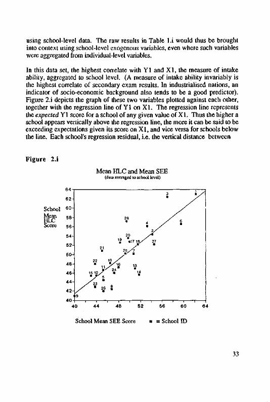
In this data set, the highest correlate with Yl and XI, the measure of intake ability, aggregated to school level. (A measure of intake ability invariably is the highest correlate of secondary exam results. In industrialised nations, an indicator of socio-economic background also tends to be a good predictor). Figure 2.i depicts the graph of these two variables plotted against each other, together with the regression line of Yl on XI. The regression line represents the expected Yl score for a school of any given value of X1. Thus the higher a school appears vertically above the regression line, the more it can be said to be exceeding expectations given its score on XI, and vice versa for schools below the line. Each school's regression residual, i.e. the vertical distance between

Figure 2.i

Mean HLC and Mean SEE (data averaged to school level)

School Mean HLC Score

6 2 -

6 0 -

58-

56-

54-

52-

50-

48-

46-

44-

42-

40-

21 •

22 10 • •

11 • 24

15 1 2 / • • • 5 23

• • 26 8

•9 1 1 1

19 •

16 •

28 •

20 • •17 18

• 25 7 • •

13 •

14 •

4 •

27 •

3 •

1 ' l

6 •

1 -• /

-r 40 52 56 60 64

School Mean SEE Score • = School ID

33

its position and the regression line (measured in terms of the y axis), can be interpreted as the relative effectiveness (or "value-added") of that school. For example, pupils in school 28 could be said to be scoring on average 7.4% higher per subject than would be expected given the average ability of its intake.

Despite the high level of correlation between these two variables(.84), two other variables were found to be sigificantly related to Y1, even after controlling for X1. These were X2 (pupil:teacher ratio) and X3 (expenditure per pupil [Tongan$]) and were included in the final, preferred regression equation.

The derived equation was as follows:

Yl = -8.8 + .98(X1) + .29(X2) + .02(X3) (R-squared = 79%)

Because this is a multi-variate model, it is not possible to depict it graphically as in the above example. However, the principle of interpreting the regression residuals as measures of relative school effectiveness remains the same, and these are reported in Table 2.i, again in rank order of schools' performance. For example, controlling for X1and X2 andX3, pupils in school 28 can now be said to be achieving on average 5.1%, higher per subject than would be expected, given their school's score on these variables. Although similar interpretations can be made for all the schools, it would be wrong to be too exact in making inter-school comparisons involving schools with similar scores, due to the standard error of the regression coefficients.

It is informative to interpret the actual coefficients of the regression equation. There is almost a 1-to-l relationship between Y1 and X1; a school wishing to increase its average HLC mark by 1% would have to recruit pupils with an average SEE mark of 1% higher than at present. The relationship between Y1 and X2 (after controlling for X1) is much less strong; by adjusting the expenditure variable, a school would have to expect to spend an extra T$50 per pupil per year in order to gain an average increase of 1% in its HLC marks. Finally, and most surprising, is that if a school were to try and improve its performance through adjusting the pupil:teacher ratio, it would need to expect to have an extra 3.4 pupils per teacher in order to increase its average HLC mark by 1%. The salient feature of this analysis however, is the overwhelming explanation of variance in schools' average HLC marks attributable to the average ability of their intake. Although the relationships between Yl and X2, X3 are statistically significant, the correlation is quite small and not too much

34

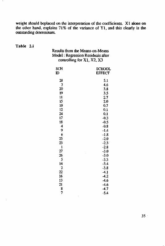
weight should beplaced on the interpretation of the coefficients. X1 alone on the other hand, explains 71% of the variance of Y1, and this clearly is the outstanding determinant.

Table 2.i Results from the Means-on-Means Model: Regression Residuals after

controlling for X1, X2, X3

SCH ID

28 3

20 19 11 15 10 12 24 17 18 4 9 6

25 23

1 27 26

5 14 2

22 16 13 21

8 7

SCHOOL EFFECT

5.1 4.6 3.8 3.5 2.7 2.0 0.7 0.1 0.1

-0.3 -0.5 -0.8 -1.4 -1.8 -2.0 -2.3 -2.8 -3.0 -3.0 -3.3 -3.4 -3.8 -4.1 -4.2 -4.6 -4.6 -4.7 -5.4

35

Critique The means-on-means model as presented here is not without some substantial deficiencies. First, because data which is essentially individual in nature (exam marks), are aggregated to the school mean level, the within-school variation on these variables automatically disappears. Consequently, any statement about school effectiveness must be very generalized, and expressed merely in terms of the average school. Were schools to have an identical and equal effect on each of their pupils, then such a situation would be acceptable. Since we do not have this knowledge, we are compelled to investigate whether schools differ in their effectiveness at different levels of ability level, socio-economic background etc. The work of Gray et al in the U.K. suggests that this is indeed a justified area for investigation, and it will be explored in the next model. As they say:

"The means-on-means model not only precludes such an investigation, but produces results which may be at the same time both highly predictable and relatively meaningless." (Gray et a 1.1986)

A second source of inadequacy of the means-on-means model is that it often fails to differentiate between distinct determinants of effectiveness. This is particularly so in the case of a balance influence which occurs when "the collective properties of a pupil body have an effect on pupil achievement over and above the effect of individual pupil characteristics" (Willms, 1985). The incidence of such effectiveness would be of great interest to the policy-maker, but the aggregated nature of the data used in this type of analysis precludes their measurement and inclusion in the model. Section (iii) demonstrates that for Tongan pupils at least, there is indeed a substantial balance effect with respect to the ability of schools' intakes.

Model 3 The "within-school regression" model.

The deficiencies of the means-on-means model can be overcome where individual-level data are available, as in Tonga. The data on 1693 pupils previously aggregated into 28 cases, can now be used in their individual format, and more meaningful analyses executed. The essence of this model is that pupil HLC marks are regressed onto their SEE marks within each school individually. However, the analysis takes place in two stages, corresponding to the "fixed" and "random" effects of the model. Before performing the within-school regressions, it is important to control for the overall effects on performance which could not be attributed to particular schools. By regressing

36

the HLC marks of each pupil (Y2) on to their SEE marks (X4), a correlation of .49 was achieved. This rose to 0.56 when two other statistically significant variables were included: school mean SEE score (X1) and school expenditure per pupil (X3). The significance of these latter two variables is of particular interest, and will be discussed more fully in the section on balance effects. The preferred model for the first part of the analysis is therefore:

Y2 = -5.96 + .33(X4) + .18(X1) + .01(X3) R-squared = 34%

This equation yields the best predicted HLC mark for a pupil if we did not know which school he was attending (but knew the information regarding the school-level variables X1 and X3).

The second stage of the analysis uses the residuals from this equation as a dependent variable. For each school individually, the variable is regressed on to pupils' individual SEE marks (X4). Each school therefore has its own regression model consisting of two parts: the first part is the above equation which it shares in common with all schools; the second part consists of its own, unique, within-school equation.

By substituting the appropriate values into a model, predicted HLC marks are obtained depending on which secondary school the (actual or hypothetical) pupil attends. For example, a predicted HLC mark for a pupil with a mean SEE mark of 50 could be derived for each of the 28 secondary schools. As alluded to earlier, this model allows different levels of ability to be substituted into the model, such that the same exercise could be repeated with pupils of any SEE mark.

These predicted HLC marks can be interpreted as school effectiveness scores/or pupils of that particular level of ability. Since each predicted mark consists of two constituent parts - that shared in common with all other schools (the fixed effects) and that which is unique to the particular school (the random effects) -only the second part of the model needs to be considered for the purposes of measuring school effectiveness. (The complete model will be returned to in due course as it has some very important characteristics.)

37

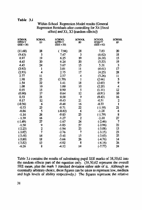
Table 3.i Within-School Regression Model results (General Regression Residuals after controlling for X4 [fixed

effect] and X1, X3 [random effects])

SCHOOL EFFECT (SEE = 38)

(11.68) (9.63) 6.97 4.65 4.43 (3.92) (2.93) 2.77 1.98 1.54 1.08 0.95 (0.90) 0.33 0.17

(-0.36) -0.73 -0.86 -1.16 -1.39 (-1.49) -1.50 (-2.23) (-3.07) (-3.48) (-3.80) (-3.82) -6.26

SCHOOL ID

28 3 19 20 24 1 4 11 25 22 10 15 17 21 12 6 23 5 26 16 27 9 2 7 14 18 13 8

SCHOOL EFFECT (SEE = 50)

( 7.96) 7.47 6.25 6.24 3.67 3.01 2.75 2.57

(1.79) 1.41 1.00 0.90 0.64 0.58 -0.43 -0.48 -0.71 (-0.82) -0.83 -1.27 -1.67 -1.85 -1.94 -2.76 -3.45 -3.66 -4.02 -4.12

SCHOOL ID

28 3 19 20 15 11 17 4 1 18 10 5 12 9 21 16 22 6 25 2 24 27 23 7 13 26 8 14

SCHOOL EFFECT (SEE = 62)

7.83 (6.62) (6.38) (5.53) 5.31 (4.61) (4.25) (3.26) (2.66) (2.65) (2.20) (1.11) (0.91) (0.43) -0.31 -0.33 (-1.18) -1.28 (-1.79) -2.20 (-2.46) (-2.96) (-3.08) (-3.15) (-3.63) (-4.76) (-6.16) (-7.77)

SCHCOL ID

20 18 15 19 3 17 28 11 5 9 4 12 10 16 2 1 21 6 8 27 7 22 13 23 25 14 26 24

Table 3.i contains the results of substituting pupil SEE marks of 38,50,62 into the random effects part of the equation only. (38,50,62 represent the overall SEE mean, plus the mark 1 standard deviation either side of it. Although an essentially arbitrary choice, these figures can be taken to represent low, medium and high levels of ability respectively.) The figures represent the relative

38

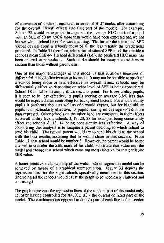
effectiveness of a school, measured in terms of HLC marks, after controlling for the overall, "fixed" effects (the first part of the model). For example, School 28 would be expected to augment the average HLC mark of a pupil with an SEE of 50 by 7.96% more than would have been expected had we not known which school he or she was attending. The further the substituted SEE values deviate from a school's mean SEE, the less reliable the predictions produced. In Table 3.i therefore, where the substituted SEE mark lies outside a school's mean SEE +/- 1 school differential (s.d.), the predicted HLC mark has been entered in parenthesis. Such marks should be interpreted with more caution than those without parenthesis.

One of the major advantages of this model is that it allows measures of differential school effectiveness to be made. It may not be sensible to speak of a school being more or less effective in overall terms; schools may be differentially effective depending on what level of SEE is being considered. School 18 in Table 3.i amply illustrates this point. For lower ability pupils, it is seen to be less effective, its pupils scoring on average 3.8% less than would be expected after controlling for background factors. For middle ability pupils it performs about as well as one would expect, but for high ability pupils it is particularly effective, its pupils scoring on average 6.62% more than expected. Other schools on the other hand are consistent in their effects across all ability levels; schools 3, 19, 20, 28 for example, being consistently effective; schools 8, 13, 14 being consistently less effective. A way of considering this analysis is to imagine a parent deciding to which school to send his child. The typical parent would try to send his child to the school with the best results, assuming that he would share in this success. From Table Li, that school would be number 3. However, the parent would be better advised to consider the SEE mark of his child, substitute that value into the model and choose that school which came out most effective for that particular SEE value.

A better intuitive understanding of the within-school regression model can be achieved by means of a graphical representation. Figure 3.i depicts the regression lines for the eight schools specifically mentioned in this section. (Including all the schools would cause the graph to be needlessly cluttered and confusing.)

The graph represents the regression lines of the random part of the model only, i.e. after having controlled for X4, X1, X3 - the overall or fixed part of the model. The continuous (as opposed to dotted) part of each line is that section

39

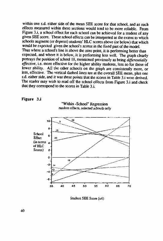
within one s.d. either side of the mean SEE score for that school, and as such effects measured within these sections would tend to be more reliable. From Figure 3.i, a school effect for each school can be achieved for a student of any given SEE score. These school effects can be interpreted as the extent to which schools augment (or depress) students' HLC scores above (or below) that which would be expected given the school's scores in the fixed part of the model. Thus where a school's line is above the zero point, it is performing better than expected, and where it is below, it is performing less well. The graph clearly portrays the position of school 18, mentioned previously as being differentially effective, i.e. more effective for the higher ability students, less so for those of lower ability. All the other schools on the graph are consistently more, or less, effective. The vertical dashed lines are at the overall SEE mean, plus one s.d. either side, and it was these points that the scores in Table 3.i were derived. The reader may wish to read off the school effects from Figure 3.i and check that they correspond to the scores in Table 3.i.

Figure 3.i "Within -School" Regression

random effects, selected schools only

10

8

School Effect 6 (in terms 4 of HLC Scores) 2

40 45 50 55 60 65 70

Student SEE Score (x4)

40

Individual subject measures Hitherto, school effectiveness has been measured in a general way, using the

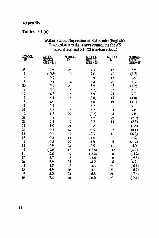
average of the three main HLC subject mark as the dependent variable. However, it is possible to perform the same analyses for HLC subjects individually, the results indicating measures of relative school effectiveness in the respective subjects. Such an exercise could provide headteachers with much more accurate information with which to evaluate departmental performance, than a mere scrutiny of raw results. Analyses were performed for the three major subjects individually: English, Maths and Tongan, and the results are presented in Table 3.ii (a-c) in the Appendix.

For these analyses, the SEE subjects (X5, X6, X7) corresponding to the respective HLC subjects were used as independent variables, rather than the mean SEE mark. The results contain some interesting features, and indicate that measuring school effective ness in a general way can conceal some large inter-subject differences. School 9 for example, is consistently effective in Tonga, but performs poorly in English and especially Maths.

Balance influence Balance influence occurs when "the collective properties of a pupil body have an effect on pupil achievement over and above the effects of individual pupil characteristics" (Willms, 1985). Such "collective properties" are multifarious, but in the research two in particular were utilised: the mean and s.d. of secondary schools' SEE intake scores. In other words, it was investigated whether the overall ability of a school's intake (as measured by the mean SEE), or the distribution of that intake (as measured by the s.d.), affected pupil performance over and above individual pupil ability. Although the latter measure was found not to be significant, the former proved to have some effect. Returning to the fixed effect part of the general model, the equation was as follows:

Y2 = -5.96 + .33 (X4) + .18 (X1) + .01 (X3) R-squared = 34%

On its own, X4 "explained" 24% of the total variance in HLC marks; adding X1 into the equation increased the amount of variance explained to 32%, which proved to be a significant increase. The interpretation of the coefficient (.18) is that a difference of 5.6% in a school's average SEE marks, yields a corresponding difference of 1% (on average) for each pupil at HLC level. Because the coefficient (and thus the relationship) is positive, pupils attending schools with a high average SEE on intake, would automatically have their

41

marks augmented at HLC level (and vice versa). The desirability, or otherwise, of selecting and grouping pupils at secondary level to maximise this effect is of course purely a matter of policy and educational philosophy. A more egalitarian system would seek to reduce the effect by achieving an equal mix of ability in all schools; a more elitist system would group pupils so as to maximise this effect, to the advantage of the more able pupils. (Which system produces better results overall is a moot point.) The author's own research in the U.K. suggested that moving from a selective (elitist) to comprehensive (egalitarian) education system affected the distribution of results, but that the mean level remained unchanged (Gray et al, 1984). It could be argued that in a small country like Tonga, maintaining a selected process which capitalises on this balance effect is justified in order to try and maximuse the number of pupils with the necessary level of qualifications required to fulfil the country's skilled manpower requirements.

Measuring the existence of balance effects is useful to both the researcher interested in determining factors of educational achievement, and to the policy­maker aiming to optimise a given policy.

Conclusion

Achieving an appropriate measure of the "value-added" factor has proved to be not such a simple task. First, appropriate data which are both valid and reliable, are required on individual pupils on both entering and leaving secondary school. This is the very minimum; ideally data on all factors thought to influence pupil attainment (e.g. sex, ethnic background, socio­economic grouping, pupil:teacher ratio, expenditure per pupil) should also be gathered. Second, it has been illustrated that it is not always appropriate to speak of school effectiveness in uni-dimensional terms, because differential levels of effectiveness often need to be taken into account

The results of research of this kind can prove to be a two-edged sword. It is necessary that effective schools are identified in order that the reasons for that effectiveness can be investigated, and these good practices introduced to all schools, thus raising the overall standard. However, it is not intended that the results be used as a criterion to judge schools as "good" or "poor", albeit this would be fairer than judging them on raw results alone. It is to be hoped that educational researchers and policy-makers would be responsible and professional

42

enough to ensue the latter path, and use the analyses as a tool for improving all school's performances.

The above analyses give an indication as to which schools are more (and less) effective at different intake levels, and by how much. They also begin to give us an understanding of how factors such as expenditure per pupil and pupil:teacher ratio affect school performance. But this is by no means the end of the story. The next step would be to insert time as a factor into the analyses, in order to test for consistency of school effects across years. Assuming an acceptable level of consistency, it would be compelling to investigate why some schools were consistently more effective (and others less effective). What is it about schools 3, 19, 20, 28 for instance that distinguishes them from schools 8, 13, 14? The first port of call in attempting to answer this question should be with the headteachers themselves, requesting explanations for their own school's elevated or modest position. It is likely that factors responsible for this difference are not easily quantifiable, and would require sensitive qualitative research into aspects such as teacher morale, headteacher's leadership skills, teaching styles, time-on-task etc. If and when these factors can be researched and operationalised, they would provide the next step forward in providing a useful model of determinants of school effectiveness.

43

Appendix

Tables 3.ii(a)

Within-School Regression Model results (English): Regression Residuals after controlling for X5

(fixed effect) and X1, X3 (random effects) SCHOOL

ID

28 1 4 3

20 14 19 5

13 15 22

2 24 25 16 21 18 17 7

12 6

11 27 26

8 23 9

10

SCHOOL EFFECT (SEE = 35)

12.9 (10.8)

9.9 9.1 5.4 5.0 4.3 4.1 4.0 3.7 3.5 1.3 1.1 1.1 1.0 0.7

-0.1 -0.2 -0.8 -0.9

(-2.6) -2.6 -2.7 -2.9 -4.5 -4.9 -5.0 -7.6

SCHOOL ID

28 3 1 4

20 5

16 15 17 19 18 22 13 2

21 14 7

11 27 24 12 9 8

25 8

26 23 10

SCHOOL EFFECT (SEE = 50)

9.3 7.6 6.9 6.4 5.9

(5.2) 3.9 (3.8) 3.8 3.7 3.2

(3.2) 3.2 2.2 1.2 0.5

-0.3 -1.4 -1.9 -2.5 (-2.6) (-3.2) -3.6 -4.2 -4.3 -5.1 -5.8

-6.0

SCHOOL ID

17 16 18 20

5 3

28 15 19 2 1 4

22 13 21

7 11 27

9 14 12 8

10 6

24 23 26 25

SCHOOL EFFECT (SEE = 65)

7.9 (6.7) 6.5 6.3

(6.2) 6.1 5.7 (4.0) (3-1) 3.1 3.0 3.0 (2.9) (2.5) (1.6) (0.1) (-0.2) -1.2

(-1.4) -4.0 (4.2) (-4.2) (-4.3) -4.7 (-6.1) (-6.7) (-7.4) (-9.4)

44

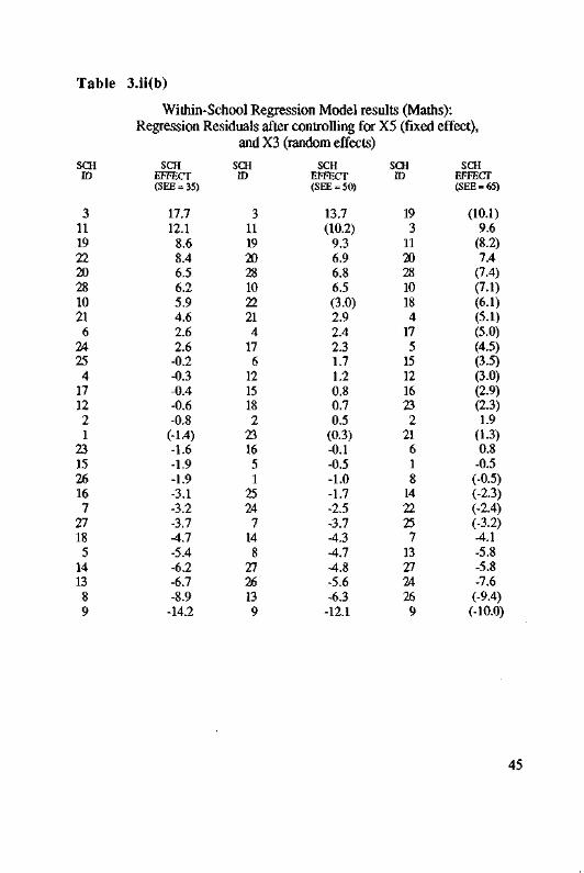
Table 3.ii(b)

Within-School Regression Model results (Maths): Regression Residuals after controlling for X5 (fixed effect),

and X3 (random effects) SCH SCH SCH SCH SCH SCH

3 11 19 22 20 28 10 21 6 24 25 4 17 12 2 1 23 15 26 16 7 27 18 5 14 13 8 9

(SEE = 35)

17.7 12.1 8.6 8.4 6.5 6.2 5.9 4.6 2.6 2.6 -0.2 -0.3 -0.4 -0.6 -0.8 (-1.4) -1.6 -1.9 -1.9 -3.1 -3.2 -3.7 -4.7 -5.4 -6.2 -6.7 -8.9 -14.2

3 11 19 20 28 10 22 21 4 17 6 12 15 18 2 23 16 5 1 25 24 7 14 8 27 26 13 9

(SEE = 50)

13.7 (10.2) 9.3 6.9 6.8 6.5 (3.0) 2.9 2.4 2.3 1.7 1.2 0.8 0.7 0.5 (0.3) -0.1 -0.5 -1.0 -1.7 -2.5 -3.7 -4.3 -4.7 4.8 -5.6 -6.3 -12.1

19 3 11 20 28 10 18 4 17 5 15 12 16 23 2 21 6 1 8 14 22 25 7 13 27 24 26 9

(SEE = 65)

(10.1) 9.6 (8.2) 7.4 (7.4) (7.1) (6.1) (5.1) (5.0) (4.5) (3.5) (3.0) (2.9) (2.3) 1.9 (1.3) 0.8 -0.5 (-0.5) (-2.3) (-2.4) (-3.2) -4.1 -5.8 -5.8 -7.6 (-9.4) (-10.0)

45

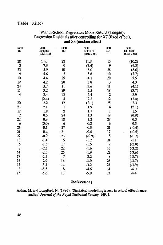
Table 3.ii(c)

Within-School Regression Mode Results (Tongan): Regression Residuals after controlling for X7 (fixed effect),

and X3 (random effect)

ID

28 3 25 9 10 19 24 11 4 1 20 23 12 2 22 6 26 21 27 18 5 7 14 17 16 15 8 13

EFFECT (SEE = 35)

14.0 7.3 5.9 5.6 4.4 4.2 3.7 3.2 2.4 (2.4) 2.2 2.1 1.8 0.5 0.3 (0.0) -0.1 -0.4 -0.9 -1.4 -1.6 -2.3 -2.5 -2.6 -2.9 -5.4 -5.5 -5.6

ID

28 9 10 3 25 20 11 19 15 4 12 1 2 24 18 6 27 21 23 5 17 22 26 7 16 14 8 13

EFFECT (SEE = 50)

11.3 (7.4) 6.0 5.8 4.1 3.8 3.6 2.5 2.4 2.2 (2.1) 1.9 1.7 1.3 1.2 -0.2 -0.3 -0.4 (-0.9) -1.2 -1.5 -1.6 -1.9 -2.2 -3.0 -3.2 -4.6 -5.0

References

ID

15 9 28 10 20 3 11 18 2 12 25 4 1 19 27 6 21 17 5 24 7 16 22 8 26 23 14 13

EFFECT (SEE = 65)

(10.2) (9.2) (8.6) (7.7) 5.5 4.3 (4.1) (3.7) 2.9 (2.4) 2.3 (2.1) 1.5 (0.9) 0.3 -0.3 (-0.4) (-0.5) (-0.7) -1.1 (-2.0) (-3.2) (-3.6) (-3.7) (-3.7) (-3.9) -4.0 -4.4

Aitkin, M. and Longford, N. (1986). 'Statistical modelling issues in school effectiveness studies', Journal of the Royal Statistical Society, 149, 1.

46

Burstein, L. (1980). 'Issues in the aggregation of data'. In Berliner, D.C. (Ed.) Review of Research in Education. Washington, D.C.: American Educational Research Association.

Cuttance, P. (1985). 'Methodological issues in the statistical analysis of data on the effectiveness of schooling', British Educational Research Journal, 11, 2, 163-179.

Goldstein, H. (1984) The methodology of school comparisons', Oxford Review of Education, 10, 1, 69-74.

Gray, J. (1981). 'A competitive edge: examination results and the probable limits of secondary school effectiveness', Educational Review, 33, 1, 25-35.

Gray, J., Jesson, D. and Jones, B. (1984). 'Predicting Differences in Examination Results between Local Education Authorities: does school organisation matter?' Oxford Review of Education, 10, 1, 45-68.

Gray, J., Jesson, D. and Jones, B. (1986). The search for a fairer way of comparing schools' examination results', Research Papers in Education, 1, 2, 91-122.

Marco, G.L. (1974). 'A comparison of selected school effectiveness measures based on longitudinal data', Journal of Educational Measurement, 11, 4, 225-234.

Ranson, S., Gray, J., Jesson, D. and Jones, B. (1986). 'Exams in context: values and power in educational accountability'. in Nuttall, D.L. (Ed.) Assessing Educational Achievement. Basingstoke: Falmer Press.

Royal Statistical Society (RSS) (1984). 'Assessment of examination performance in different types of school: a general discussion'. Journal of Royal Statistical Society: A, 147,569-581.

Rutter, M. Maughan, B. Mortimore, P. Ouston, J. with Smith, A. (1979). Fifteen Thousand Hours : Secondary Schools and their Effects on Children. London: Open Books.

Willms, J.D. (1984). 'A multilevel approach for assigning school effectiveness scores', paper presented to the ESRC Seminar on 'Analysing Educational Data on Schooling', Edinburgh.

Willms, J.D. (1985). 'The balance thesis: contextual effects of ability on pupils' O-grade examination results', Oxford Review of Education, 11,1.

Willms, J.D. and Cuttance, P. (1985). School effects in Scottish secondary schools', British Journal of Sociology of Education, 6,3.

47