1

The Valuation of Payers’ Swaption

Kun Woo Kim*1 Hong Jae Lee**2

1. Introduction

Swap options or swaption are option on interest rate swap and are another increasingly popular type of interest rate option. Swaption give the holder the right to enter into a certain interest rate swap at a certain time in the future. The most large financial institutions are also prepared to sell their clients swaptions or buy swaptions from their clients.

Swaptions provide companies with a guarantee that the fixed rate of interest they * Professor, Kyung Hee University, Seoul, Korea

The purpose of this study include to perform data analysis by fitting with the measurement

of the interest rate derivatives products, European style and Bermudan style swaptions. And the other purpose is to understand the model mathematically. Moreover, during the calibration process, we should construct a sense of understanding the major classes to the model(i.e. short rate, replicating portfolio, state price and swaption value). Therefore wedemonstrate on the basis of which the driving factor is the short rate and that the logarithm ofthe short rate is normally distributed.

It can be seen that result in our study: First, among the three tree-values, the discrepancy of the value of ∆t =1/4 is the smallest,

Second, among the three tree-values, the discrepancy of the value of ∆t =1/2 is the greatest,Third, both the values of ∆t =1 and ∆t =1/2 are smaller than the Black-value.

It says that early exercise opportunity can be checked easily by means of tree model. Italso shows that replicating strategy can be easily understood by tree model. Finally, the tree-values of the European payers swaption are compared with the Black-value. The result shows that the smallest ∆t gives value with the smallest discrepancy. However, the greatest∆t does not give value with the greatest discrepancy.

Abstract

2

will pay on a loan at some future time will not exceed some level. They are an alternative to forward swaps(or called deffered swaps). Forward swaps involve no up-front cost but have the disadvantage of obligating the company to enter into a swap agreement. With a swaption, the company is able to benefit from favorable interest rate movements.

A swaption can be regarded as an option to exchange a fixed rate bond for the principal amount of the swap. If a swaption gives the holder the right to pay fixed and received floating, it is a put option on the fixed rate bond with strike price equal to the principal. If a swaption gives the holder the right to pay floating and receive fixed, it is a call option on the fixed-rate bond with a strike price equal to the principal.

The model presented by Black, Dermon and Toy(1990), which is the fitting model with the analysis of the European style and Bermudan style swaptions in this paper, is commonly described as a one-factor binomial state lattice model. It assumes that the driving factor is the short rate and that the logarithm of the short rate is normally distributed. The lognormal distribution assumption for the term structure of interest is the most natural way to exclude negative spot and forward rates. However, imposing this assumption on the continuously compounded interest rate has a serious drawback: rates explode and expected rollover returns are infinite even if the rollover period is arbitrarily short.

Heath, Jarrow, and Morton (1992)) a lognormal volatility structure of the form σ(t; T; f):=f(t; T) γ(t; T); where f(t; T) denotes the instantaneous forward rate valid at time t for the infinitesimal time interval [T; T + dt] and γ(t; T) is deterministic, is inconsistent. It was already shown by Morton(1988) that the resulting rates become infinite with positive probability. This implies zero prices for contingent claims with positive payoff and hence arbitrage opportunities.

Jamshidian (1996a) proposed using simple or effective rates as the primary process for a term structure model seems natural, rather than as a secondary process derived from instantaneous rates.

The binomial short rate model of Sandmann and Sondermann((1989, 92, 93b) was the first model of effective interest rates. Although this discrete model looks very similar to the Black, Derman, and Toy(1990)(BDT)model, its limit behaviour is quite different. In the limit of the BDT-model the continuously compounded instantaneous

3

rate rc(t) follows a lognormal diffusion. In the limit of the Sandmann-Sondermann model rc(t) follows a diffusion which is

neither normal nor lognormal, but a dynamic combination of both with the following properties: for small values of rc(t) the diffusion process approaches a lognormal diffusion, thus generating positive rates, whereas for large values of rc(t) the diffusion approaches a normal diffusion process, generating stable finite expected returns and futures values.

Vasicek(1997) stated on an equilibrium characterization of the term structure. His model incorporates mean reversion. In his research, he demonstrated that the short rate is pulled to a level b at rate a . And dzσ is a normally probability distributed (NPD) stochastic term. In his model, r can become negative.

Jamshidian(1997) has shown that options on zero-coupon bonds can be valued using Vasicek’s model(1977). He also shown that the prices of options on coupon-bearing bonds can be obtained from the prices of options on zero-coupon bonds in a one-factor model.

Cox, Ingersoll and Ross(1985) have proposed an alternative model where rate are always non-negative. The model of the risk-neutral process for r has the same mean-reverting drift as Vasicek, but σ is proportional to r . This means that as the short rate increase, it’s standard deviation increases.

In this paper, We presents an binomial short rate approximate formula and BDT European payer swaptions in the lognormal Libor market model. The lognormal Libor market model has been introduced by Musiela and Rutkowski(1997) and Jamshidian (1997) especially to price and hedge Libor and swap derivatives. In the lognormal Libor market model, a closed form formula for European swaptions is not available.

Approximate formulae and Monte Carlo simulation methods for European swaptions in the lognormal Libor market model are developed by many authors, such as Brace, Gatarek, and Musiela (1997); Brace, Dun, and Barton (1998); Rebonato (1999); and Sidenius (2000).

This paper is organized as follows. Section 2 Pricing model for European Swaption. Section 3 formulates the European payer swaption and Bermuda payer swaption pricing problem under the forward swap measure. Section 4 derives an approximate formula and Which presents numerical results. Finally, section 5 gives some

4

conclusions.

2. Pricing Model for European Swaptions.

A swaption is a combination of the following two financial instruments: Interest Rate Swap (IRS) and Option. Swaptions first came into vogue in the mid-1980s in the US on the back of structured bonds tagged with a callable option issued by borrowers. With a callable bond, a borrower issues a fixed-rate bond which he may call at par from the investor at a specific date(s) in the future. In return for the issuer having the right to call the bond issue at par, investors are offered an enhanced yield.

Bond issuers often issue an IRS in conjunction with the bond issue in order to change their interest profile from fixed to floating. Swaptions are then required by the issuer as protection to terminate all or part of the original IRS in the event of the bonds being put or called. A Swaption(Swap Option) reserves the right for its holder to purchase a swap at a prescribed time and interest rate in the future (European Option).

The holder of such a call option has the right, but not the obligation to pay fixed in exchange for variable interest rate. Therefore, this option is also known as "Payer Swaption". The holder of the equivalent put option has the right, but not the obligation to receive interest at a fixed rate (Receiver Swaption) and pay variable.

Actually, a swaption is an option on a forward interest rate. Like interest rate swaps, swaptions are used to mitigate the effects of unfavorable interest rate fluctuations at a future date. The premium paid by the holder of a swaption can more or less be considered as insurance against interest rate movements. In this way, businesses are able to guarantee risk limits in interest rates.

The purpose of Our studies include to perform data analysis by fitting with the measurement of the interest rate derivatives products, European style and Bermudan style swaptions on GBP, as well as understanding the model mathematically. Moreover, during the calibration process, we should construct a sense of understanding the major classes to the model(i.e. short rate, replicating portfolio, state price and swaption value). Therefore we start our discussion on the basis of which the driving factor is the short rate and that the logarithm of the short rate is normally distributed.

5

In Our paper we demonstrate on the term structure model that are constructed by specifying the behavior of the short term interest rate, r(or U(i)). The models for pricing interest rate options make the assumption that probability distribution of interest rate(IRD), a bond price at a future point on time is lognormal. They are widely used for valuing instrument such as European bond options and European swaption. However, they have limitations. They do not provide a description of the stochastic behavior of interest rate. Consequently, they can’t be used for valuing IRD such American style swap options.

The alternative studies for overcoming this limitations which are known as a term structure model. Therefore, Our study demonstrate on the basis of term structure models that are constructed by specifying the behavior of the short-term interest rate. The short rate can be described in a risk-neutral world by an Ito process of the form. A one-factor model that is used for analysis implies that all rates move in the same direction over any short time interval, but not that they all move by same amount.

Let t1 < … < tn represent the coupon dates for the swap and t0 = T. In deriving a pricing formula, we look at the swap underlying the swaption. The swap begins on the expiration date(T) of the swaption - this coincides with the first cash flows and ends at time tn. The swap comprises payments at floating interest rate Xv and payments at fixed interest rate Xf , relative to the n cash flows.

Notation:

T : expiry date of Option F : forward swap rate B(0, ti): discount factor from date ti, down to 0 Xv: variable interest rate Xf : fixed interest rate σ: volatility of swap K: Strike rate Rfix: Market swap rate at time T

The variable interest rate payments are based on a bench mark(mostly LIBOR) at

time tk, a notional principal amount L and n interest periods(ti− ti-1). The fixed payments

6

are based on the strike rate K, as well as same notional principal amount and periods. At each date ti, the interest rate Rfix shall be compared with the Strike rate K.

In case Rfix > K, the fixed interest payer gets paid a balance of L (Rfix− K)(ti−ti−1). Otherwise this balance goes to the variable interest payer. The swap rate Rfix satisfies the following equation.

LtTBLttRtTB n

n

iiifixi )),(1()(),(

11 −=−∑

=− (Equation 1)

The left hand side of the above equation represents the value of the fixed payments at

the rate of Rfix as of time T. The right hand side, on the other hand, represents the value of variable payments. Take note that the present value at variable interest rate will be equal to the notional principal amount.

The holder of an European swaption has the right to pay the fixed rate K and to receive a floating rate(payer swaption). In the case that Rfix > K, it means for the holder a value of

LttKtTBLtTBXXn

iiiinfv ∑

=−−−−=−

11 )(),()),(1(

LttKtTBLttRtTB

n

iiii

n

iiifixi ∑∑

=−

=− −−−=

11

11 )(),()(),(

LtttTBKRn

iiiifix ∑

=−−−=

11))(,()( (Equation 2)

According to the Black Model (1976), the option value at time 0 is as follows:

B(0, ti)(ti− ti-1)L[FN(d1)− K N(d2)] (Equation 3)

Where

( )T

TKF

dσ

σ 2

12

1ln += ,

( )Td

T

TKF

d σσ

σ−=

−= 1

2

22

1ln (Equation 4)

7

The forward swap rate F is obtained by replacing B(T, ti) with F(T, ti) = [B(0, ti)/B(0,

T )]. The value of the swap CE itself is the summation over all individual call options, i.e. over all i. And we get: CE = LA[FN(d1)/ KN(d2)] (Equation 5)

Whereby

∑=

−−=n

iiii tttBA

11 ))(,0( (Equation 6)

For an European receiver swaption in like manner, if K > Rfix the the following holds:

LtTBLttKtTBXX n

n

iiiivf )),(1()(),(

11 −−−=− ∑

=−

LttRtTBLttKtTB

n

iiifixi

n

iiii ∑∑

=−

=− −−−=

11

11 )(),()(),(

LtttTBRKn

iiiifix ∑

=−−−=

11 ))(,()( (Equation 7)

The ith term corresponds to the value of an European put option with expiry date T

and coupon date ti. L(ti− ti−1)(K− Rfix)+ (Equation 8)

According to the Black Model (1976), the option value at time 0 is as follows:

B(0, ti)(ti− ti-1)L[K N(-d2)−FN(-d1)] (Equation 9)

whereby F, d1, d2 are as defined above, d1 and d2 are as introduced in (Equation 4).

The forward swap rate F is obtained by substituting B(T, ti) with F(T, ti)=[B(0, ti)/B(0, T )]. The swap value PE is the summation over all individual put options, i.e. over all i. And we get:

8

PE = L A[K N(-d2)/FN(d1)] (Equation 10)

whereby

∑=

−−=n

iiii tttBA

11 ))(,0( (Equation 11)

3. Methodology

One of the main advantages of the Black-Derman-Toy(1990) model is that it is a lognormal model that is able to capture a realistic term structure of interest rate volatilities. To accomplish this feature, the short-term rate volatility is allowed to vary over time, and the drift in interest rate movements depends on the level of rates. While interest rate mean reversion is not modeled explicitly, this property is introduced through the term structure of volatilities. Hence, the extent to which the drift term depends on the level of rates depends on the local volatility process. In other words, the mean reversion is endogenous to the model. Therefore, no additional degree of freedom is required for the mean reversion term, and the BDT SDE(stochastic differential equations)can be relatively easily approximated using the binomial tree approach.

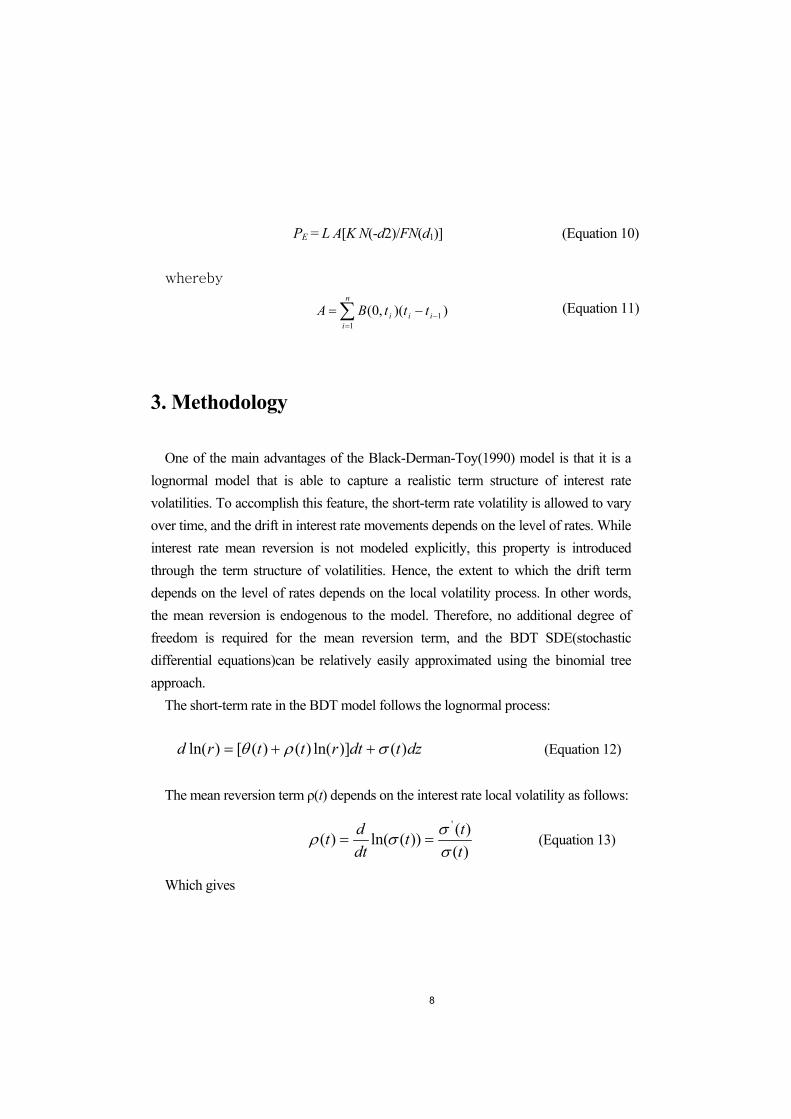
The short-term rate in the BDT model follows the lognormal process:

dztdtrttrd )()]ln()()([)ln( σρθ ++= (Equation 12)

The mean reversion term ρ(t) depends on the interest rate local volatility as follows:

)()())(ln()(

'

ttt

dtdt

σσσρ == (Equation 13)

Which gives

9

dztdtr

tttrd )()ln()()()()ln(

'

σσσθ +

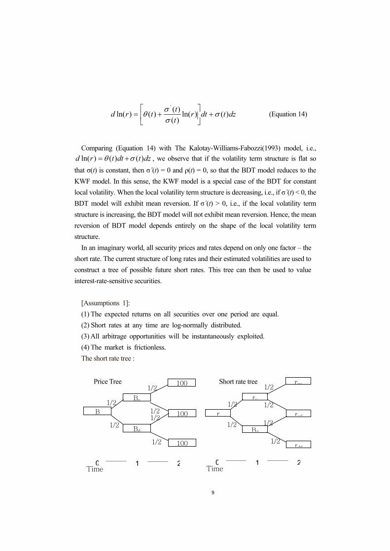
+= (Equation 14)

Comparing (Equation 14) with The Kalotay-Williams-Fabozzi(1993) model, i.e.,

dztdttrd )()()ln( σθ += , we observe that if the volatility term structure is flat so that σ(t) is constant, then σ´(t) = 0 and ρ(t) = 0, so that the BDT model reduces to the KWF model. In this sense, the KWF model is a special case of the BDT for constant local volatility. When the local volatility term structure is decreasing, i.e., if σ´(t) < 0, the BDT model will exhibit mean reversion. If σ´(t) > 0, i.e., if the local volatility term structure is increasing, the BDT model will not exhibit mean reversion. Hence, the mean reversion of BDT model depends entirely on the shape of the local volatility term structure.

In an imaginary world, all security prices and rates depend on only one factor – the short rate. The current structure of long rates and their estimated volatilities are used to construct a tree of possible future short rates. This tree can then be used to value interest-rate-sensitive securities.

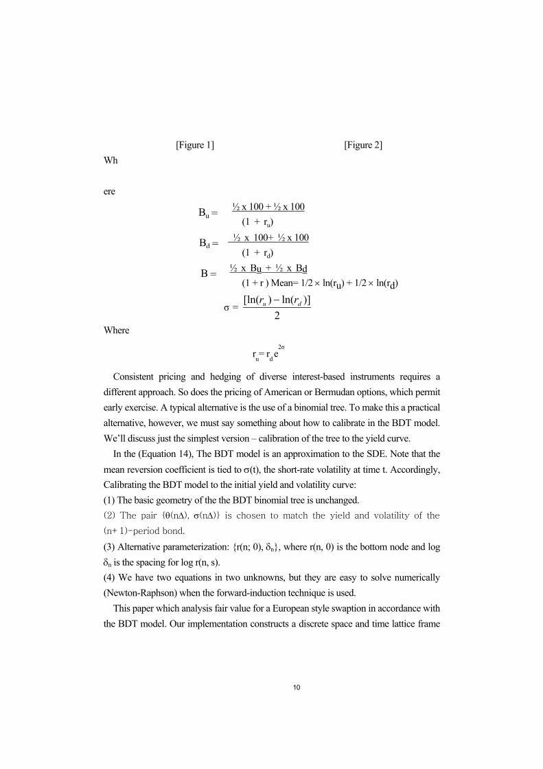
[Assumptions 1]: (1) The expected returns on all securities over one period are equal. (2) Short rates at any time are log-normally distributed. (3) All arbitrage opportunities will be instantaneously exploited. (4) The market is frictionless. The short rate tree :

Bd

100

100

100B

Bu

1/2

1/2

1/2 1/2

1/2

1/2

0 1 2Time

Bd

ruu

rdd

rudr

ru

1/2

1/2 1/2

1/2

1/2

1/2

0 1 2Time

Price Tree Short rate tree

10

[Figure 1] [Figure 2] Wh ere

½ x 100 + ½ x 100 (1 + ru)

½ x 100+ ½ x 100 (1 + rd)

½ x Bu + ½ x Bd (1 + r ) Mean= 1/2 × ln(ru) + 1/2 × ln(rd)

σ = 2

)]ln()[ln( du rr −

Where

ru= rd e2σ

Consistent pricing and hedging of diverse interest-based instruments requires a different approach. So does the pricing of American or Bermudan options, which permit early exercise. A typical alternative is the use of a binomial tree. To make this a practical alternative, however, we must say something about how to calibrate in the BDT model. We’ll discuss just the simplest version – calibration of the tree to the yield curve.

In the (Equation 14), The BDT model is an approximation to the SDE. Note that the mean reversion coefficient is tied to σ(t), the short-rate volatility at time t. Accordingly, Calibrating the BDT model to the initial yield and volatility curve: (1) The basic geometry of the the BDT binomial tree is unchanged. (2) The pair {θ(n∆), σ(n∆)} is chosen to match the yield and volatility of the

(n+1)-period bond.

(3) Alternative parameterization: {r(n; 0), δn}, where r(n, 0) is the bottom node and log δn is the spacing for log r(n, s). (4) We have two equations in two unknowns, but they are easy to solve numerically (Newton-Raphson) when the forward-induction technique is used.

This paper which analysis fair value for a European style swaption in accordance with the BDT model. Our implementation constructs a discrete space and time lattice frame

Bu =

Bd =

B =

11

which is arbitrage free at every time-step corresponding to an observable point on the input yield curve. Forward arbitrage free lattices are generated for any other rates required. Paths through the lattice are then sampled to get monthly rates.

<Table 1> Valuation of European style swaption

Argument Description Value date Swaption settlement date Effective date Swap effective date Maturity date Swap maturity date Principal Swaption notional amount Coupon Strike price Frequency Swap frequency Accrual method Actual/365 Swaption type Pay/Receive fixed Holiday table GBP holiday table Discount factor curve (calculated from yield curve generation

function) Interpolation method Linear Mean reversion constant (calculated from calibration process) Rate volatility (calculated from calibration process)

Calculate fair value for a Bermudan style swaption in accordance with the BDT model.

<Table 2> Valuation of Bermudan style swaption

Argument Description Value date Swaption settlement date Effective date Swap effective date Maturity date Swap maturity date Principal Swaption notional amount Coupon Strike price Frequency Swap frequency Accrual method Actual/365 Swaption type Pay/Receive fixed Holiday table GBP holiday table Discount factor curve (calculated from yield curve generation

function)

12

Interpolation method Linear First call date First exercise call date Last call date Last exercise call date Mean reversion constant (calculated from calibration process) Rate volatility (calculated from calibration process)

Notations used in this research;

α: number of discount bond purchased in the replicating portfolio β: number of discount bond sold in the replicating portfolio σ: volatility of the discount bond yield d(i, j): discount factor at time i and state j P(i, j, T): discount bond value at time i, state j, and matures at time T P(i, T): discount bond value at time i and matures at time T r(i, j) or U(i, j): short rate at time i and state j Q(i,j): state price at time i and state j V(i, j): swaption value at time i and state j

In the original BDT paper, short rates are found by backward induction. The

proposed procedure is conceptually straight forward. However, it is proved that the calculation will become very cumbersome as the tree grows larger and larger.3 Therefore, the tricky part in implementing the BDT model is to construct the short rate tree efficiently.

Alternative methods have been suggested, and the one we used in this research involves the estimation of state prices Q(i,j) across the tree and median U(i) of the short rate distribution at time i4. This procedure is preferred to the backward induction since it avoids traversing the whole tree again and again; consequently greatly reduces the calculation.

The calculation process is implemented through Excel worksheet and the Euro-denominated discount bond prices are obtained from arbitrary data source(e.g. zero

3 See Rebonato p.194-199. 4 For detail, see Clewlow p.233-240 and Chalasani p.12-20

13

rate and discount factor). Forward discount factors are calculated from zero discount factors. Forward interest rates are obtained from forward discount factors.

By using Black-76 model and the technique of bootstrapping, individual caplet volatilities are obtained. Caplet volatilities are used for BDT implementation. It can be analysis from the supplementary Excel worksheet that we have constructed 3 short rate trees with different ∆t, where ∆t=1 year, 1/2 year and 1/4 year. The trees are built until the maturity of the underlying swap.

The value of the payer swaption becomes

Payer Swaption= )]()([),0( 2101

dNRdNFtPmL

X

m

ii −∑

=

Defining A as the value of a contract that pays 1/m at times )1( mniti ≤≤ , the

value of the swaption becomes

)]()([ 210 dNRdNFLA X−

where

TTXSd

σσ 2/)/ln( 2

1+

=

Tdd σ−= 12 where

T: maturity date of the swaption

0F : forward swap rate

σ: volatility of 0F

L: notional value of the underlying swap m: payment number per annum under swap A: value of the swap

The value of forward swap rate becomes

14

)4,0()3,0()2,0()4,0()1,0(

0 PPPPPF++

−=

In this paper, we will demonstrate that a swaption can be created synthetically by a

portfolio of discount bonds. The analysis process is;

Let Π(0, 0) be a portfolio consisting of :

Long α (0, 0) × P(0, 0, 1) Short β (0, 0) × P(0, 0, 2)

At time 1, portfolio Π(0, 0) will become either

Π(1, 1)= α (0, 0) + β (0, 0) × P(1, 1, 2)

or

Π(1, -1)= α (0, 0) + β (0, 0) × P(1, -1, 2) If

Π(1, 1) = V(1, 1), Π(1, -1) = V(1, -1) Since

V(1, 1)= d(1, 1) ×0.5[V(2,2) +V(2,0)] V(1, -1)= d(1, -1) ×0.5[V(2,-2) +V(2,0)] P(1, 1, 1)= 1 P(1, 1, 2)= 0.97753

Then α (0, 0)= V(1, 1)-β(0, 0)×d(1, 1) β (0, 0)= [V(1, 1)-V(1,-1)] / [d(1, 1)+d(1, -1)] Π(0, 0)= V(0, 0)= d(0, 0)×0.5×[V(1, 1) +V(1, -1)]

Note that Π(0, 0) is exactly equal to V(0, 0) and provides the same expected payoff.

15

Therefore, Π(0, 0) replicates the swaption. Now, consider that there are 4 paths from time 0 to time 2 :

Up – Up, Up – Down, Down–Up, Down–Down Let’s choose on path, for example, Up – Up The replication portfolio Π(0, 0) : Π(0, 0)= α (0, 0)×P(0, 0, 1) + β (0, 0) × P(1, 1, 2)

Its cost at time 0 is 0.02016, and its payoff at time 1 is 0.03036. The replicating portfolio Π(1, 1) is Π(1, 1)= α (1, 1) *P(1, 1, 2)+ β (1, 1) * P(1, 1, 3)

Since α (1, 1)= 6.1246 β (1, 1)= -6.24817 P(1, 1, 2)= 0.97753 P(1, 1, 3)= 0.95334 Π(1, 1)= 0.03036

That means, in order to form portfolio Π(1, 1), together with borrowing from P(1, 1,

3) additional 0.03036 is needed. However, the payoff from the previous replicating portfolio, Π(1, 1), exactly satisfies this need. Therefore, no additional money is needed from the portfolio holder. In other words, the replicating strategy is self-financing.

4. The Empirical Analysis and The Results

1) Valuation of Payers’ swaption; [American and Black]

In this section, we will use the short rate trees described in the last section to value a European payers’ swaption and a Bermudan payers’ swaption. We have made use of Excel worksheet for empirical study.

16

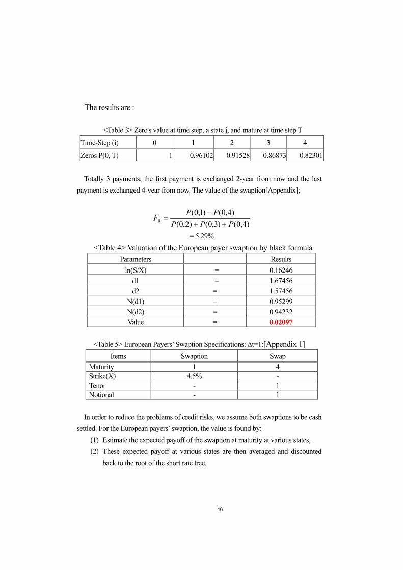
The results are :

<Table 3> Zero's value at time step, a state j, and mature at time step T Time-Step (i) 0 1 2 3 4

Zeros P(0, T) 1 0.96102 0.91528 0.86873 0.82301

Totally 3 payments; the first payment is exchanged 2-year from now and the last payment is exchanged 4-year from now. The value of the swaption[Appendix];

)4,0()3,0()2,0()4,0()1,0(

0 PPPPPF++

−=

= 5.29% <Table 4> Valuation of the European payer swaption by black formula

Parameters Results ln(S/X) = 0.16246

d1 = 1.67456 d2 = 1.57456

N(d1) = 0.95299 N(d2) = 0.94232 Value = 0.02097

<Table 5> European Payers’ Swaption Specifications: ∆t=1:[Appendix 1]

Items Swaption Swap Maturity 1 4 Strike(X) 4.5% - Tenor - 1 Notional - 1

In order to reduce the problems of credit risks, we assume both swaptions to be cash

settled. For the European payers’ swaption, the value is found by: (1) Estimate the expected payoff of the swaption at maturity at various states, (2) These expected payoff at various states are then averaged and discounted

back to the root of the short rate tree.

17

We have valued the European payers swaption by three short rate trees, and the results are:

<Table 6> Zero's value at time step, a state j, and mature at time step T; P(1, j, T)

I 0 1 2 3 4 Total

ΣQ(1, 1, T) 1 0.94785 0.89518 0.84359 2.68662

ΣQ(1, -1, T) 1 0.95690 0.91291 0.86937 2.73919 (1) Expected swap rate S(1, j) for the underlying swap[Appendix]:

S(1,1) = ∑−

),1,1()4,1,1(1

TPP

= 5.82%

S(1,-1) = ∑ −

−−),1,1()4,1,1(1

TPP

= 4.77%

(2) Payoff Function of the Swaption at Maturity :

Max [ S(1, j) - X ] * ΣP(1, 1, T)

(3) Expected Payoff of the Swaption, V(1, j), at Maturity[Appendix] :

V(1, 1) = (5.82% - 4.5%) * ΣP(1, 1, T) = 0.03551 V(1, -1) = (4.77% - 4.5%) * ΣP(1, -1, T) = 0.00736 V(0, 0) =d(0, 0)*0.5*[V(1, 1)*V(1, -1)]=0.02060

Replicating the Swaption Position;

Let Π(0, 0) be a portfolio consisting of :

Long α P(0, 0, 1) Short β P(0, 0, 2)

18

At time 1, portfolio Π will become either

Π(1, 1) = α + β P(1, 1, 2) or

Π(1, -1) = α + β P(1, -1, 2) If

Π(1, 1) = V(1, 1), Π(1, -1) = V(1, -1) Then

α = 2.98514 β = -3.11191 Π(0, 0) = 0.02060

where Π(0, 0) is exactly equal to V(0, 0) and provides the same expected payoff.

<Table 7> European Payers’ Swaption Specifications: ∆t=1/2: [Appendix 2]

Swaption Swap

Maturity (year) 2 Maturity (year) 8 Strike (X) 4.5% Tenor 1 Notional 1

<Table 8> Zero's value at time step 2, a state j, and mature at time step T; P(2, j, T)

I 0 1 2 … 8 Total

ΣQ(2, 2, j, T) 1 … 5.43180

ΣQ(2, 0, j, T) 1 … 5.50180

ΣQ(2, -2, j, T) 1 … 5.56372 Expected swap rate S(2, j) for the underlying swap;

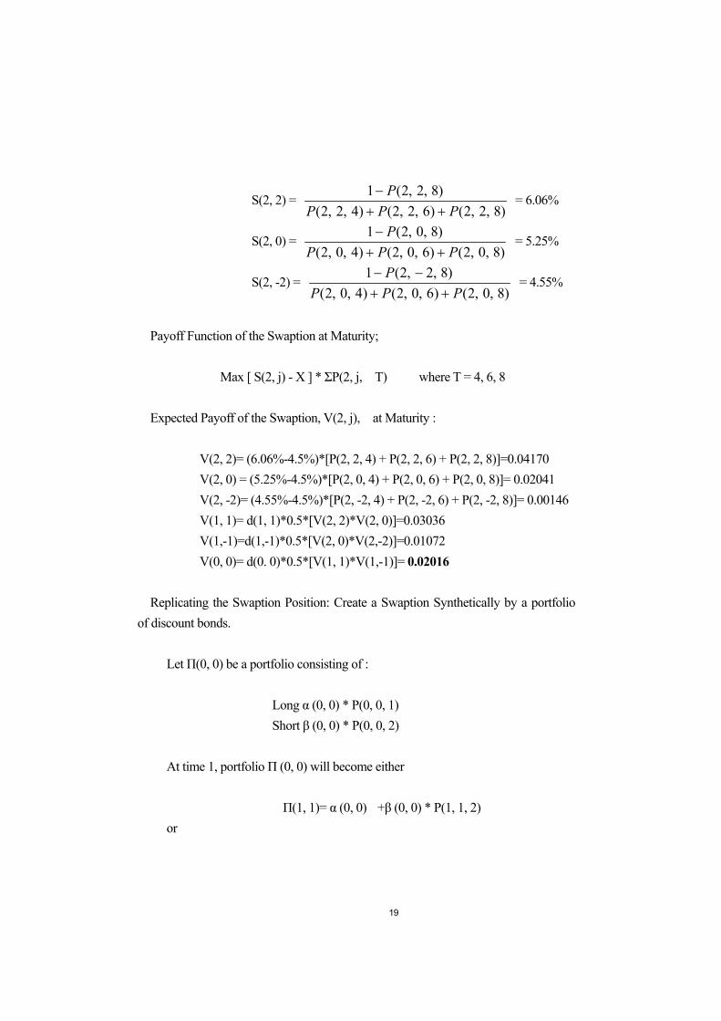
19

S(2, 2) = )8,2,2()6,2,2()4,2,2(

)8,2,2(1PPP

P++

− = 6.06%

S(2, 0) = )8,0,2()6,0,2()4,0,2(

)8,0,2(1PPP

P++

− = 5.25%

S(2, -2) = )8,0,2()6,0,2()4,0,2(

)8,2,2(1PPP

P++

−− = 4.55%

Payoff Function of the Swaption at Maturity;

Max [ S(2, j) - X ] * ΣP(2, j, T) where T = 4, 6, 8 Expected Payoff of the Swaption, V(2, j), at Maturity :

V(2, 2)= (6.06%-4.5%)*[P(2, 2, 4) + P(2, 2, 6) + P(2, 2, 8)]=0.04170 V(2, 0) = (5.25%-4.5%)*[P(2, 0, 4) + P(2, 0, 6) + P(2, 0, 8)]= 0.02041 V(2, -2)= (4.55%-4.5%)*[P(2, -2, 4) + P(2, -2, 6) + P(2, -2, 8)]= 0.00146 V(1, 1)= d(1, 1)*0.5*[V(2, 2)*V(2, 0)]=0.03036 V(1,-1)=d(1,-1)*0.5*[V(2, 0)*V(2,-2)]=0.01072 V(0, 0)= d(0. 0)*0.5*[V(1, 1)*V(1,-1)]= 0.02016

Replicating the Swaption Position: Create a Swaption Synthetically by a portfolio

of discount bonds. Let Π(0, 0) be a portfolio consisting of :

Long α (0, 0) * P(0, 0, 1) Short β (0, 0) * P(0, 0, 2)

At time 1, portfolio Π (0, 0) will become either

Π(1, 1)= α (0, 0) +β (0, 0) * P(1, 1, 2)

or

20

Π(1, -1) = α (0, 0)+β (0, 0) * P(1, -1, 2) If

Π(1, 1) = V(1, 1), Π(1, -1) = V(1, -1) Since

V(1, 1)= 0.03036 V(1, -1)= 0.01072 P(1, 1, 1)= 1 P(1, 1, 2)= 0.97753

Then α (0, 0)= 6.63914 β (0, 0)=-6.76067 Π(0, 0)= 0.02016

Note that Π(0, 0) is exactly equal to V(0, 0) and provides the same expected

payoff. Therefore, Π(0, 0) replicates the swaption.

[Self-Financing Principle] Now, consider that there are 4 paths from time 0 to time 2;

Up – Up, Up – Down, Down – Up, Down – Down

Let’s choose on path, for example, Up – Up The replicating portfolio Π(0, 0):

Π(0, 0)= α (0, 0) *P(0, 0, 1)+β (0, 0) * P(1, 1, 2)

Its cost at time 0 is 0.02016, and its payoff at time 1 is 0.03036. The replicating portfolio Π(1, 1) is

Π(1, 1)= α (1, 1) *P(1, 1, 2)+β (1, 1) * P(1, 1, 3)

= 5.98700+(-5.95664)= 0.03036 Since

21

α (1, 1)= 6.1246 β (1, 1)= -6.24817 P(1, 1, 2)= 0.97753 P(1, 1, 3)= 0.95334 Π(1, 1)= 0.03036

That means, in order to form portfolio Π(1, 1), together with borrowing

from P(1, 1, 3) additional 0.03036 is needed. However, the payoff from the previous replicating portfolio, Π(1, 1), exactly satisfies this need. Therefore, no additional money is needed from the portfolio holder. In other words, the replicating strategy is self-financing.

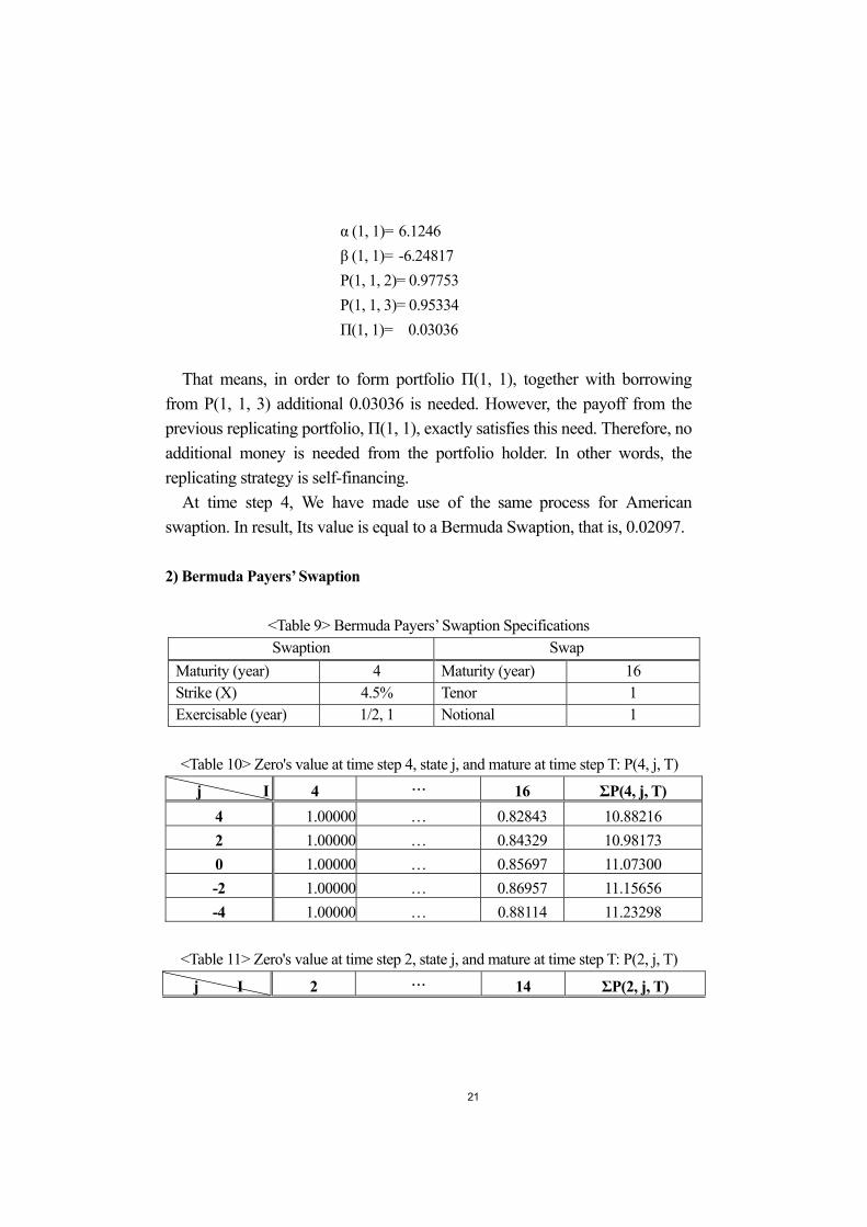
At time step 4, We have made use of the same process for American swaption. In result, Its value is equal to a Bermuda Swaption, that is, 0.02097.

2) Bermuda Payers’ Swaption

<Table 9> Bermuda Payers’ Swaption Specifications Swaption Swap

Maturity (year) 4 Maturity (year) 16 Strike (X) 4.5% Tenor 1 Exercisable (year) 1/2, 1 Notional 1 <Table 10> Zero's value at time step 4, state j, and mature at time step T: P(4, j, T)

j I 4 … 16 ΣP(4, j, T) 4 1.00000 … 0.82843 10.88216 2 1.00000 … 0.84329 10.98173 0 1.00000 … 0.85697 11.07300 -2 1.00000 … 0.86957 11.15656 -4 1.00000 … 0.88114 11.23298

<Table 11> Zero's value at time step 2, state j, and mature at time step T: P(2, j, T)

j I 2 … 14 ΣP(2, j, T)

22

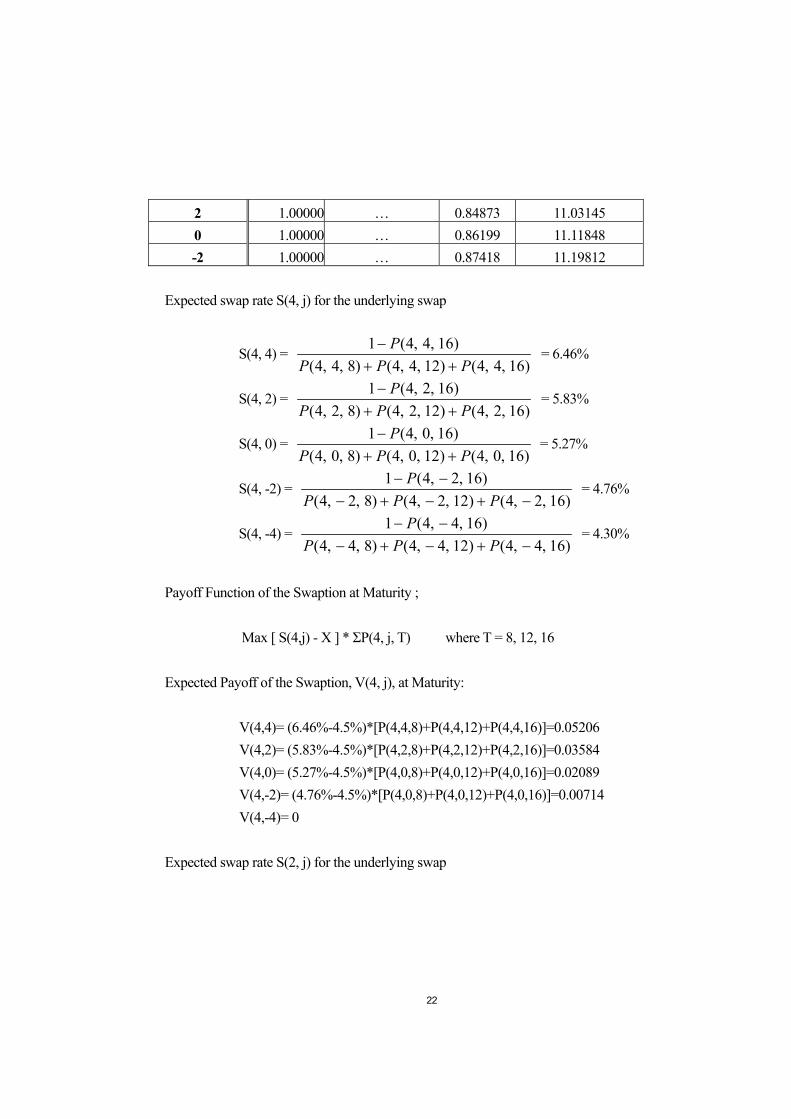
2 1.00000 … 0.84873 11.03145 0 1.00000 … 0.86199 11.11848 -2 1.00000 … 0.87418 11.19812

Expected swap rate S(4, j) for the underlying swap

S(4, 4) = )16,4,4()12,4,4()8,4,4(

)16,4,4(1PPP

P++

− = 6.46%

S(4, 2) = )16,2,4()12,2,4()8,2,4(

)16,2,4(1PPP

P++

− = 5.83%

S(4, 0) = )16,0,4()12,0,4()8,0,4(

)16,0,4(1PPP

P++

− = 5.27%

S(4, -2) = )16,2,4()12,2,4()8,2,4(

)16,2,4(1−+−+−

−−PPP

P = 4.76%

S(4, -4) = )16,4,4()12,4,4()8,4,4(

)16,4,4(1−+−+−

−−PPP

P = 4.30%

Payoff Function of the Swaption at Maturity ;

Max [ S(4,j) - X ] * ΣP(4, j, T) where T = 8, 12, 16 Expected Payoff of the Swaption, V(4, j), at Maturity:

V(4,4)= (6.46%-4.5%)*[P(4,4,8)+P(4,4,12)+P(4,4,16)]=0.05206 V(4,2)= (5.83%-4.5%)*[P(4,2,8)+P(4,2,12)+P(4,2,16)]=0.03584 V(4,0)= (5.27%-4.5%)*[P(4,0,8)+P(4,0,12)+P(4,0,16)]=0.02089 V(4,-2)= (4.76%-4.5%)*[P(4,0,8)+P(4,0,12)+P(4,0,16)]=0.00714 V(4,-4)= 0

Expected swap rate S(2, j) for the underlying swap

23

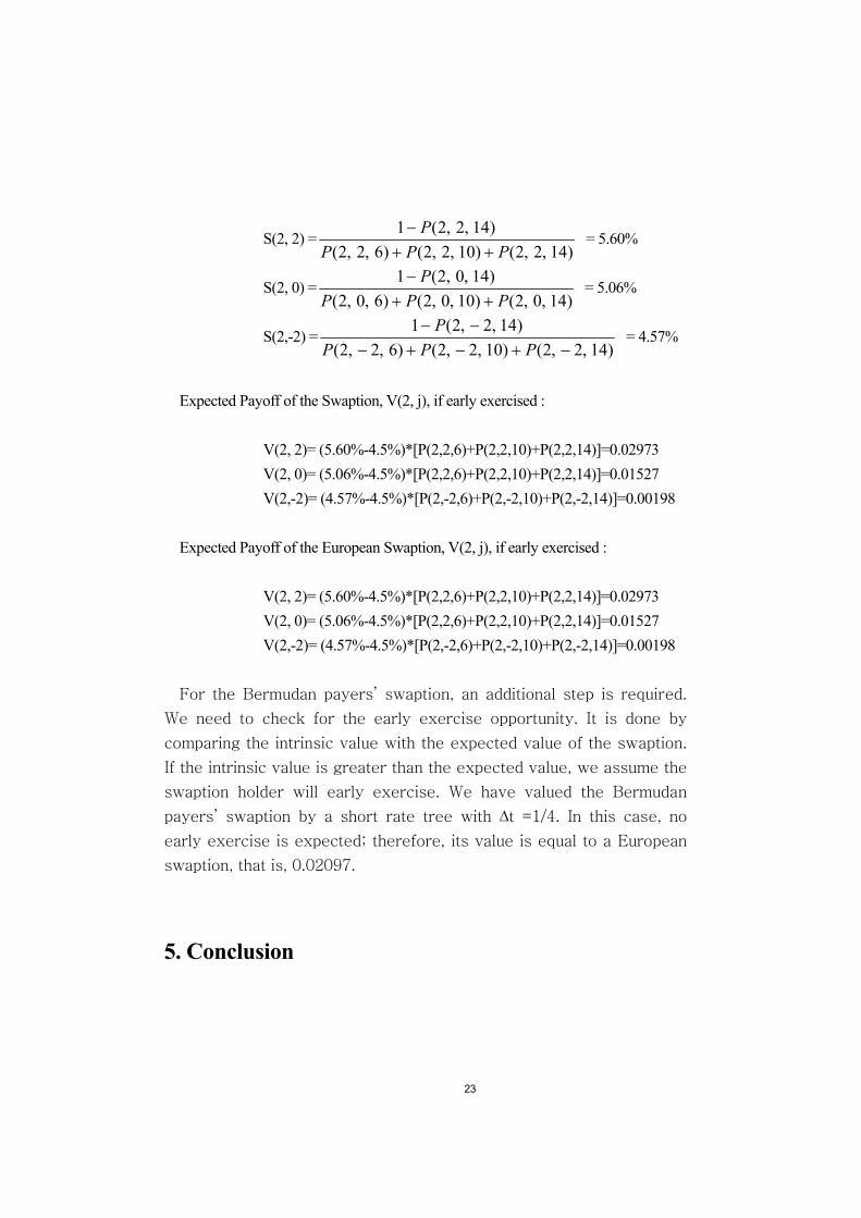
S(2, 2) =)14,2,2()10,2,2()6,2,2(

)14,2,2(1PPP

P++

− = 5.60%

S(2, 0) =)14,0,2()10,0,2()6,0,2(

)14,0,2(1PPP

P++

− = 5.06%

S(2,-2) =)14,2,2()10,2,2()6,2,2(

)14,2,2(1−+−+−

−−PPP

P = 4.57%

Expected Payoff of the Swaption, V(2, j), if early exercised :

V(2, 2)= (5.60%-4.5%)*[P(2,2,6)+P(2,2,10)+P(2,2,14)]=0.02973 V(2, 0)= (5.06%-4.5%)*[P(2,2,6)+P(2,2,10)+P(2,2,14)]=0.01527 V(2,-2)= (4.57%-4.5%)*[P(2,-2,6)+P(2,-2,10)+P(2,-2,14)]=0.00198

Expected Payoff of the European Swaption, V(2, j), if early exercised :

V(2, 2)= (5.60%-4.5%)*[P(2,2,6)+P(2,2,10)+P(2,2,14)]=0.02973 V(2, 0)= (5.06%-4.5%)*[P(2,2,6)+P(2,2,10)+P(2,2,14)]=0.01527 V(2,-2)= (4.57%-4.5%)*[P(2,-2,6)+P(2,-2,10)+P(2,-2,14)]=0.00198

For the Bermudan payers’ swaption, an additional step is required.

We need to check for the early exercise opportunity. It is done by

comparing the intrinsic value with the expected value of the swaption.

If the intrinsic value is greater than the expected value, we assume the

swaption holder will early exercise. We have valued the Bermudan

payers’ swaption by a short rate tree with ∆t =1/4. In this case, no

early exercise is expected; therefore, its value is equal to a European

swaption, that is, 0.02097.

5. Conclusion

24

In this study, we use a simple method to implement the BDT model. The resulted short rate trees are then used to value a European payers swaption and a Bermudan payers swaption.

<Table 13> The value of the European swaption by short rate trees ∆t =1 ∆t =1/2 ∆t =1/4

Value 0.02060 0.02016 0.02097

In before result, we have estimated the value of the European swaption by short rate

trees with different time steps. In this time, we will compare these values (tree-values) with the value given by the Black formulae (Black-value).

The Black-value of the European swaption is 0.02097. The comparison of the tree values with the Black-value is shown in the following table.

<Table 14> The Black value of the European swaption ∆t =1 ∆t =1/2 ∆t =1/4

Tree-value 0.02060 0.02016 0.02097 Discrepancy -1.76% -3.86% 0%

It can be seen that result: First, Among the three tree-values, the discrepancy of the value of ∆t =1/4 is the

smallest, Second, among the three tree-values, the discrepancy of the value of ∆t =1/2 is the greatest, Third, both the values of ∆t =1 and ∆t =1/2 are smaller than the Black-value.

It says that early exercise opportunity can be checked easily by means of tree model. It also shows that replicating strategy can be easily understood by tree model. Finally, the tree-values of the European payers swaption are compared with the Black-value. The result shows that the smallest ∆t gives value with the smallest discrepancy. However, the greatest ∆t does not give value with the greatest discrepancy.

25

[Reference]

Andersen, L. (2000), “A Simple Approach to the Pricing of Bermudan Swaptions in the

Multifactor LIBOR Market Model,” Journal of Computational Finance, 3, 5–32.

Black, F., E. Derman, and W. Toy. (1990), “A One-Factor Model of Interest Rates and its Application to Treasury Bond Options,” Financial Analysts Journal, 46, 33–39.

Black, F., and P. Karasinski.(1991), “Bond and Option Pricing when Short Rates are Lognormal,” Financial Analysts Journal, 47, 52–59.

Brace, A., and Gatarek, D., and Musiela, M. (1997), The market model of interest rate dynamics. Mathematical Finance, 7, 127–55.

Brace, A., and Dun, T., and Barton, G. (1998). Towards a central interest rate model. ICBI Global Derivatives Conference, Paris, April.

Cox, J. C., J. E. Ingersoll, Jr. and S. A. Ross. (1985) “A Theory of the Term Structure of Interest Rates.”Econometrica 53, 385-407.

Heath, D. R., R. Jarrow and A. Morton. (1992) “Bond Pricing and the Term Structure of Interest Rates: A New Methodology for Contingent Claims Valuation.” Econometrica 60, 77-105.

Heath, D. R., R. Jarrow and A. Morton. (1990),“Bond Pricing and the Term Structure of Interest Rates: A Discrete Time Application.” Journal of Financial and Quantitative Analysis 25, 419-440.

Heath, D., R. Jarrow and A. Morton. (1990), “Contingent Claims Valuation with a Random Evolution of Interest Rates.” Review of Futures Markets 9, 54-76.

Hull, J. and A. White. (1993), “One-Factor Interest Rate Models and the Valuation of Interest-Rate Derivative Securities.” Journal of Financial and Quantitative Analysis 28, 235-254.

.(Fall, 1994), “Numerical Procedures for Implementing Term Structure Models I: Single-Factor Models.” The Journal of Derivatives 2 (Fall), 7-16.

26

.(Winter, 1994), “Numerical Procedures for Implementing Term Structure ModelsII: Two-Factor Models.” The Journal of Derivatives 2 (Winter), 37-48.

.(Spring, 1996), “Using Hull-White Interest Rate Trees.” The Journal of Derivatives 3,26-36.

Jamshidian, F. (1989), “An Exact Bond Option Formula.” The Journal of Finance 44, 205-209.

.(1997), “LIBOR and swap market models and measures.” Finance and Stochastics, 1, 293–330.

Kalotay, A., G. Williams, and F. Fabozzi. (May/June 1993), “A Model for the Valuation of Bonds and Embedded Options.” Financial Analysts Journal, pp. 35-46.

Musiela, M., and Rutkowski, M. (1997). Continuous-time term structure models: Forward measure approach. Finance and Stochastics, 1, 261–91.

Ritchken, Peter and L. Sankarasubramanian. (1995), “Volatility Structures of Forward Rates and the Dynamics of the Term Structure.” Mathematical Finance, 55-72.

. (Fall, 1995), “The Importance of Forward Rate Volatility Structures in Pricing Interest Rate-Sensitive Claims.” The Journal of Derivatives 3 (Fall, 1995), 25-41.

Rebonato, R. (1999). On the pricing implications of the joint lognormal assumption for the swaption and cap markets. Journal of Computational Finance, 2(3), 57–76.

Sidenius, J. (2000). LIBOR market models in practice. Journal of Computational Finance, 3(3), 5–26.

Vasicek, O. (1977) ,“An Equilibrium Characterization of the Term Structure.” Journal of Financial Economics 5, 177-188.

27

[Appendix 1]

I. European Payers’ Swaption Specifications: ∆t=1

<Table-1> Value of the Swaption & Discount Bond Value

Value of the Swaption Discount Bond Value Variables Results Variables Results ln(S/X) 0.16246 F0

* 5.29% d1 1.67456 P(0, 0) 1 d2 1.57456 P(0, 1) 0.96102

N(d1) 0.95299 P(0, 2) 0.91528 N(d2) 0.94232 P(0, 3) 0.86873 Value 0.02097 P(0, 4) 0.82301

‘*’: forward swap rate, F0=[P(0,1)-P(0,4)]/[P(0,2)+P(0,3)+P(0,4)]

‘**’:

<Table-2> Matched Price % change under time step 4: Fixed Volatility Time-Step (i) 0 1 2 3 4

○1 Zeros P(0, T) 1 0.96102 0.91528 0.86873 0.82301 ○2 U(i) - 4.98% 5.30% 5.49% - ○3 Implied P(0, 0, T) or

∑Q(I,j)×d(I, j) - 0.91525 0.86881 0.82310 -

○4 Matched(%): ○1t+1-○2t

- 0.0028% (0.0078%) (0.0085%) -

28

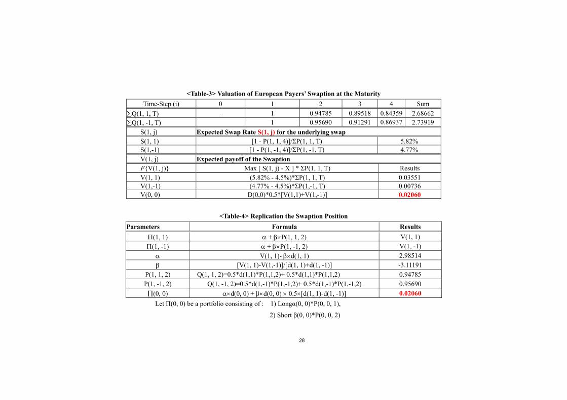
<Table-3> Valuation of European Payers’ Swaption at the Maturity Time-Step (i) 0 1 2 3 4 Sum

∑Q(1, 1, T) - 1 0.94785 0.89518 0.84359 2.68662 ∑Q(1, -1, T) 1 0.95690 0.91291 0.86937 2.73919

S(1, j) Expected Swap Rate S(1, j) for the underlying swap S(1, 1) [1 - P(1, 1, 4)]/ΣP(1, 1, T) 5.82% S(1,-1) [1 - P(1, -1, 4)]/ΣP(1, -1, T) 4.77% V(1, j) Expected payoff of the Swaption

F{V(1, j)} Max [ S(1, j) - X ] * ΣP(1, 1, T) Results V(1, 1) (5.82% - 4.5%)*ΣP(1, 1, T) 0.03551 V(1,-1) (4.77% - 4.5%)*ΣP(1,-1, T) 0.00736 V(0, 0) D(0,0)*0.5*[V(1,1)+V(1,-1)] 0.02060

<Table-4> Replication the Swaption Position Parameters Formula Results

Π(1, 1) α + β×P(1, 1, 2) V(1, 1) Π(1, -1) α + β×P(1, -1, 2) V(1, -1)

α V(1, 1)- β×d(1, 1) 2.98514 β [V(1, 1)-V(1,-1)]/[d(1, 1)+d(1, -1)] -3.11191

P(1, 1, 2) Q(1, 1, 2)=0.5*d(1,1)*P(1,1,2)+ 0.5*d(1,1)*P(1,1,2) 0.94785 P(1, -1, 2) Q(1, -1, 2)=0.5*d(1,-1)*P(1,-1,2)+ 0.5*d(1,-1)*P(1,-1,2) 0.95690 ∏(0, 0) α×d(0, 0) + β×d(0, 0) × 0.5×[d(1, 1)-d(1, -1)] 0.02060

Let Π(0, 0) be a portfolio consisting of : 1) Longα(0, 0)*P(0, 0, 1),

2) Short β(0, 0)*P(0, 0, 2)

29

[Appendix 2]

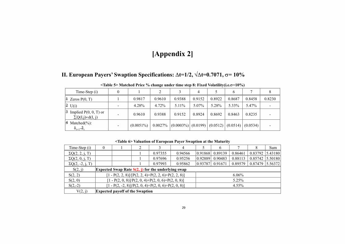
II. European Payers’ Swaption Specifications: ∆t=1/2, √∆t=0.7071, σ= 10%

<Table 5> Matched Price % change under time step 8: Fixed Volatility(i.e.σ=10%)

Time-Step (i) 0 1 2 3 4 5 6 7 8

○1 Zeros P(0, T) 1 0.9817 0.9610 0.9388 0.9152 0.8922 0.8687 0.8458 0.8230

○2 U(i) - 4.28% 4.72% 5.11% 5.07% 5.28% 5.33% 5.47% - ○3 Implied P(0, 0, T) or

∑Q(I,j)×d(I, j) - 0.9610 0.9388 0.9152 0.8924 0.8692 0.8463 0.8235 -

○4 Matched(%): ○1t+1-○2t

- (0.0051%) 0.0027% (0.0003%) (0.0199) (0.0512) (0.0514) (0.0534) -

<Table 6> Valuation of European Payer Swaption at the Maturity Time-Step (i) 0 1 2 3 4 5 6 7 8 Sum ΣQ(2, 2, j, T) 1 0.97355 0.94566 0.91868 0.89139 0.86461 0.83792 5.43180ΣQ(2, 0, j, T) 1 0.97696 0.95256 0.92889 0.90483 0.88113 0.85742 5.50180ΣQ(2, -2, j, T) 1 0.97993 0.95862 0.93787 0.91671 0.89579 0.87479 5.56372

S(2, j) Expected Swap Rate S(2, j) for the underlying swap S(2, 2) [1 - P(2, 2, 8)]/[P(2, 2, 4)+P(2, 2, 6)+P(2, 2, 8)] 6.06% S(2, 0) [1 - P(2, 0, 8)]/P(2, 0, 4)+P(2, 0, 6)+P(2, 0, 8)] 5.25% S(2,-2) [1 - P(2, -2, 8)]/P(2, 0, 4)+P(2, 0, 6)+P(2, 0, 8)] 4.55%

V(2, j) Expected payoff of the Swaption

30

f{V(2, j)} Max [ S(2, j) - X ] × ΣP(2, j, T) where T = 4, 6, 8 Results V(2, 2) (6.06%-4.5%)× [P(2, 2, 4) + P(2, 2, 6) + P(2, 2, 8)] 0.04170 V(2,0) (5.25%-4.5%)× [P(2, 0, 4) + P(2, 0, 6) + P(2, 0, 8)] 0.02041 V(2,-2) (4.55%-4.5%)× [P(2, -2, 4) + P(2, -2, 6) + P(2, -2, 8)] 0.00146 V(1, 1) d(1, 1) ×0.5[V(2,2) + V(2,0)] 0.03036 V(1,-1 ) d(1, -1) ×0.5[V(2,0) + V(2,-2)] 0.01072 V(0, 0) d(0, 0) ×0.5×[V(1, 1) + V(1, -1)] 0.02016

<Table-7> Replication the Swaption Position Parameters Formula Results

Π(1, 1) α(0, 0) + β(0, 0)×P(1, 1, 2) V(1, 1) Π(1, -1) α(0, 0) + β(0, 0)×P(1,-1, 2) V(1, -1) α(0, 0) V(1, 1)-β(0, 0)×d(1, 1) 6.63914 β(0, 0) [V(1, 1)-V(1,-1)] / [d(1, 1)+d(1, -1)] -6.76067 P(1, 1, 2) [∏(1, 1)- α(0, 0)]/ β(0, 0) 0.97753 P(1,-1, 2) [∏(1,-1)- α(0, 0)]/ β(0, 0) 0.98044 ∏(0, 0) α×d(0, 0) + β×d(0, 0) × 0.5×[d(1, 1)-d(1, -1)] 0.02016

Let Π(0, 0) be a portfolio consisting of : 1) Longα(0, 0)*P(0, 0, 1), 2) Short β(0, 0)*P(0, 0, 2)

<Table-8> Self-Financing Results Parameters Formula

Up-Up Down-Down α(1, 1) V(2, 2)-β(1, 1)×d(2, 2) 6.1246 - β(1, 1) [V(2, 2)-V(2, 0)] / [d(2, 2)+d(2, 0)] -6.24817 - α(1, -1) V(2, -2)-β(1, -1)×d(2, -2) - 6.23765

31

β(1, -1) [V(2, 0)-V(2,-2)] / [d(2, 0)+d(2, -2)] - -6.36389 P(0, 0, 1) d(0, 0) ×0.5×[d(1, 1)+d(1,-1)] 0.98170 - P(1, 1, 2) [∏(1, 1)- α(0, 0)]/ β(0, 0) 0.97753 - P(1, 1, 3) d(1, 1) ×0.5×[d(2, 2)+d(2, 0)] 0.95334 - P(1, -1, 2) [∏(1,-1)- α(0, 0)]/ β(0, 0) - 0.98044 P(1, -1, 3) d(1, -1) ×0.5×[d(2, 0)+d(2, -2)] - 0.95931 Π(0, 0) α(0, 0) ×P(0, 0, 1)+ β(0, 0) ×P(0, 0, 1) 0.02016 - Π(1, 1) α(1, 1) ×P(1, 1, 2)+ β(1, 1)×P(1, 1, 3) 0.03036 - Π(1, -1) α(1,-1) ×P(1, -1, 2)+ β(1,-1)×P(1,-1, 3) - 0.01072

[Appendix 3]

III. European Payers’ Swaption Specifications: ∆t=1/4, √∆t=0.5, σ= 10%

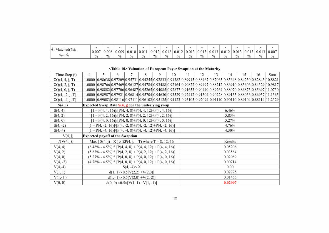
<Table 9> Matched Price % change under time step 8: Fixed Volatility(i.e.σ=10%)

Time-Step (i) 1 2 3 4 5 6 7 8 9 10 11 12 13 14 15 16

○1 Zeros P(0, T) 0.9912 0.9817 0.9716 0.9610 0.9502 0.9389 0.9271 0.9153 0.9039 0.8922 0.8804 0.8687 0.8574 0.8459 0.8343 0.8230

○2 U(i) 3.83% 4.15% 4.38% 4.52% 4.81% 5.04% 5.11% 4.99% 5.17% 5.31% 5.32% 5.23% 5.37% 5.46% 5.42% 3.83%○3 Implied P(0, 0, T) or

∑Q(I,j)×d(I, j) 0.9818 0.9717 0.9611 0.9503 0.9390 0.9272 0.9154 0.9040 0.8924 0.8806 0.8689 0.8575 0.8460 0.8345 0.8231 0.9818

32

○4 Matched(%): ○1t+1-○2t

-0.007

%

-0.008

%

-0.009

%

-0.010

%

-0.011

%

-0.012

%

-0.012

%

-0.012

%

-0.013

%

-0.013

%

-0.013

%

-0.012

%

-0.013

%

-0.013

%

-0.013

%

-0.007

%

<Table 10> Valuation of European Payer Swaption at the Maturity Time-Step (i) 4 5 6 7 8 9 10 11 12 13 14 15 16 SumΣQ(4, 4, j, T) 1.0000 0.98638 0.97209 0.95731 0.94255 0.92833 0.91382 0.89915 0.88467 0.87065 0.85648 0.84230 0.82843 10.8821ΣQ(4, 2, j, T) 1.0000 0.98766 0.97469 0.96127 0.94784 0.93488 0.92164 0.90822 0.89497 0.88212 0.86910 0.85606 0.84329 10.9817ΣQ(4, 0, j, T) 1.0000 0.98882 0.97706 0.96487 0.95265 0.94085 0.92877 0.91653 0.90440 0.89264 0.88070 0.86873 0.85697 11.0730ΣQ(4, -2, j, T) 1.0000 0.98987 0.97921 0.96814 0.95704 0.94630 0.93529 0.92412 0.91304 0.90228 0.89135 0.88036 0.86957 11.1565ΣQ(4, -4, j, T) 1.0000 0.99083 0.98116 0.97111 0.96102 0.95125 0.94123 0.93105 0.92094 0.91110 0.90110 0.89104 0.88114 11.2329

S(4, j) Expected Swap Rate S(4, j) for the underlying swap S(4, 4) [1 – P(4, 4, 16)]/[P(4, 4, 8)+P(4, 4, 12)+P(4, 4, 16)] 6.46% S(4, 2) [1 – P(4, 2, 16)]/[P(4, 2, 8)+P(4, 2, 12)+P(4, 2, 16)] 5.83% S(4, 0) [1 – P(4, 0, 16)]/[P(4, 0, 8)+P(4, 0, 12)+P(4, 0, 16)] 5.27% S(4, -2) [1 – P(4, -2, 16)]/[P(4, -2, 8)+P(4, -2, 12)+P(4, -2, 16)] 4.76% S(4,-4) [1 – P(4, -4, 16)]/[P(4, -4, 8)+P(4, -4, 12)+P(4, -4, 16)] 4.30%

V(4, j) Expected payoff of the Swaption f{V(4, j)} Max [ S(4, j) - X ] × ΣP(4, j, T) where T = 8, 12, 16 Results

V(4, 4) (6.46% - 4.5%) * [P(4, 4, 8) + P(4, 4, 12) + P(4, 4, 16)] 0.05206 V(4, 2) (5.83% - 4.5%) * [P(4, 2, 8) + P(4, 2, 12) + P(4, 2, 16)] 0.03584 V(4, 0) (5.27% - 4.5%) * [P(4, 0, 8) + P(4, 0, 12) + P(4, 0, 16)] 0.02089 V(4, -2) (4.76% - 4.5%) * [P(4, 0, 8) + P(4, 0, 12) + P(4, 0, 16)] 0.00714 V(4,-4) S(4, -4)< X 0.00 V(1, 1) d(1, 1) ×0.5[V(2,2) +V(2,0)] 0.02775 V(1,-1 ) d(1, -1) ×0.5[V(2,0) +V(2,-2)] 0.01455 V(0, 0) d(0, 0) ×0.5×[V(1, 1) +V(1, -1)] 0.02097

33

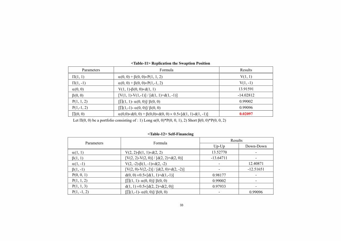
<Table-11> Replication the Swaption Position

Parameters Formula Results

Π(1, 1) α(0, 0) + β(0, 0)×P(1, 1, 2) V(1, 1) Π(1, -1) α(0, 0) + β(0, 0)×P(1,-1, 2) V(1, -1) α(0, 0) V(1, 1)-β(0, 0)×d(1, 1) 13.91591 β(0, 0) [V(1, 1)-V(1,-1)] / [d(1, 1)+d(1, -1)] -14.02812 P(1, 1, 2) [∏(1, 1)- α(0, 0)]/ β(0, 0) 0.99002 P(1,-1, 2) [∏(1,-1)- α(0, 0)]/ β(0, 0) 0.99096 ∏(0, 0) α(0,0)×d(0, 0) + β(0,0)×d(0, 0) × 0.5×[d(1, 1)-d(1, -1)] 0.02097 Let Π(0, 0) be a portfolio consisting of : 1) Long α(0, 0)*P(0, 0, 1), 2) Short β(0, 0)*P(0, 0, 2)

<Table-12> Self-Financing Results Parameters Formula

Up-Up Down-Down α(1, 1) V(2, 2)-β(1, 1)×d(2, 2) 13.52770 - β(1, 1) [V(2, 2)-V(2, 0)] / [d(2, 2)+d(2, 0)] -13.64711 - α(1, -1) V(2, -2)-β(1, -1)×d(2, -2) - 12.40871 β(1, -1) [V(2, 0)-V(2,-2)] / [d(2, 0)+d(2, -2)] - -12.51651 P(0, 0, 1) d(0, 0) ×0.5×[d(1, 1)+d(1,-1)] 0.98177 - P(1, 1, 2) [∏(1, 1)- α(0, 0)]/ β(0, 0) 0.99002 - P(1, 1, 3) d(1, 1) ×0.5×[d(2, 2)+d(2, 0)] 0.97933 - P(1, -1, 2) [∏(1,-1)- α(0, 0)]/ β(0, 0) - 0.99096

34

P(1, -1, 3) d(1, -1) ×0.5×[d(2, 0)+d(2, -2)] - 0.98127 Π(0, 0) α(0, 0) ×P(0, 0, 1)+ β(0, 0) ×P(0, 0, 1) 0.02097 - Π(1, 1) α(1, 1) ×P(1, 1, 2)+ β(1, 1)×P(1, 1, 3) 0.02775 - Π(1, -1) α(1,-1) ×P(1, -1, 2)+ β(1,-1)×P(1,-1, 3) - 0.01455

[Appendix 4]

V. Bermuda Payers’ Swaption Specifications: ∆t=1/4, √∆t=0.5, σ= 10%

<Table 13> Valuation of European Payer Swaption at the Maturity Time-Step (i) 4 5 6 7 8 9 10 11 12 13 14 15 16 SumΣQ(4, 4, j, T) 1.0000 0.98638 0.97209 0.95731 0.94255 0.92833 0.91382 0.89915 0.88467 0.87065 0.85648 0.84230 0.82843 10.8821ΣQ(4, 2, j, T) 1.0000 0.98766 0.97469 0.96127 0.94784 0.93488 0.92164 0.90822 0.89497 0.88212 0.86910 0.85606 0.84329 10.9817ΣQ(4, 0, j, T) 1.0000 0.98882 0.97706 0.96487 0.95265 0.94085 0.92877 0.91653 0.90440 0.89264 0.88070 0.86873 0.85697 11.0730ΣQ(4, -2, j, T) 1.0000 0.98987 0.97921 0.96814 0.95704 0.94630 0.93529 0.92412 0.91304 0.90228 0.89135 0.88036 0.86957 11.1565ΣQ(4, -4, j, T) 1.0000 0.99083 0.98116 0.97111 0.96102 0.95125 0.94123 0.93105 0.92094 0.91110 0.90110 0.89104 0.88114 11.2329Time-Step (i) 2 3 4 5 6 7 8 9 10 11 12 13 14 SumΣQ(2, 2, j, T) 1.00000 0.98866 0.97684 0.96476 0.95206 0.93892 0.92577 0.91309 0.90013 0.88700 0.87403 0.86146 0.84873 11.0315 ΣQ(2, 0, j, T) 1.00000 0.98973 0.97901 0.96804 0.95650 0.94453 0.93255 0.92097 0.90913 0.89712 0.88523 0.87369 0.86199 11.1185 ΣQ(2, -2, j, T) 1.00000 0.99070 0.98098 0.97102 0.96053 0.94965 0.93874 0.92818 0.91736 0.90638 0.89549 0.88492 0.87418 11.1981

S(4, j) Expected Swap Rate S(4, j) for the underlying swap S(4, 4) [1 – P(4, 4, 16)]/[P(4, 4, 8)+P(4, 4, 12)+P(4, 4, 16)] 6.46% S(4, 2) [1 – P(4, 2, 16)]/[P(4, 2, 8)+P(4, 2, 12)+P(4, 2, 16)] 5.83% S(4, 0) [1 – P(4, 0, 16)]/[P(4, 0, 8)+P(4, 0, 12)+P(4, 0, 16)] 5.27% S(4, -2) [1 – P(4, -2, 16)]/[P(4, -2, 8)+ P(4, -2, 12)+ P(4, -2, 16)] 4.76%

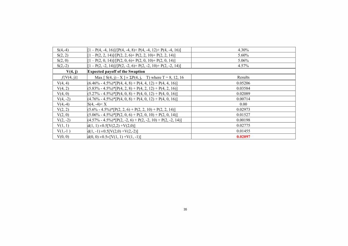
35

S(4,-4) [1 – P(4, -4, 16)]/[P(4, -4, 8)+ P(4, -4, 12)+ P(4, -4, 16)] 4.30% S(2, 2) [1 – P(2, 2, 14)]/[P(2, 2, 6)+ P(2, 2, 10)+ P(2, 2, 14)] 5.60% S(2, 0) [1 – P(2, 0, 14)]/[P(2, 0, 6)+ P(2, 0, 10)+ P(2, 0, 14)] 5.06% S(2,-2) [1 – P(2, -2, 14)]/[P(2, -2, 6)+ P(2, -2, 10)+ P(2, -2, 14)] 4.57%

V(4, j) Expected payoff of the Swaption f{V(4, j)} Max [ S(4, j) - X ] × ΣP(4, j, T) where T = 8, 12, 16 Results

V(4, 4) (6.46% - 4.5%)*[P(4, 4, 8) + P(4, 4, 12) + P(4, 4, 16)] 0.05206 V(4, 2) (5.83% - 4.5%)*[P(4, 2, 8) + P(4, 2, 12) + P(4, 2, 16)] 0.03584 V(4, 0) (5.27% - 4.5%)*[P(4, 0, 8) + P(4, 0, 12) + P(4, 0, 16)] 0.02089 V(4, -2) (4.76% - 4.5%)*[P(4, 0, 8) + P(4, 0, 12) + P(4, 0, 16)] 0.00714 V(4,-4) S(4, -4)< X 0.00 V(2, 2) (5.6% - 4.5%)*[P(2, 2, 6) + P(2, 2, 10) + P(2, 2, 14)] 0.02973 V(2, 0) (5.06% - 4.5%)*[P(2, 0, 6) + P(2, 0, 10) + P(2, 0, 14)] 0.01527 V(2, -2) (4.57% - 4.5%)*[P(2, -2, 6) + P(2, -2, 10) + P(2, -2, 14)] 0.00198 V(1, 1) d(1, 1) ×0.5[V(2,2) +V(2,0)] 0.02775 V(1,-1 ) d(1, -1) ×0.5[V(2,0) +V(2,-2)] 0.01455 V(0, 0) d(0, 0) ×0.5×[V(1, 1) +V(1, -1)] 0.02097