1

The Valuation of Multidimensional American Real Options using Computer-based Simulation

Gonzalo Cortazar*, Miguel Gravet*, Jorge Urzua*

Departamento de Ingeniería Industrial y de Sistemas, Pontificia Universidad Católica de Chile, Vicuña Mackenna 4860, Santiago, Chile

________________________________________________________________________________________

Abstract In this paper we show how a multidimensional American real option may be solved using a computer-based simulation procedure. We implement an approach originally proposed for a financial option and show how it can be used in a much more complex setting. We extend a well-known natural resource real option model, originally solved using finite difference methods, to include a more realistic 3 factor stochastic process for commodity prices, more in line with current research. We show how complexity may be reduced by adequately choosing the implementation variables. Numerical results show that the procedure may be successfully used for multidimensional models, notably expanding the applicability of the real options approach. Scope and purpose Even though there has been an increasing literature on the benefits of using the contingent claim approach to value real assets, limitations on solving procedures and computing power have often forced academics and practitioners to simplify these real option models to a level in which they loose relevance for real-world decision making. Real option models present a higher challenge than their financial option counterparts because of two main reasons: First, many real options have a longer maturity which makes risk modeling critical and may force considering many risk factors as opposed to the classic Black and Scholes one-factor model. Second, many times real investments have a more complex set of interacting American options available, making them more difficult to value. In recent years new approaches for solving American options have been proposed which, coupled with an increasing availability of computing power, have been successfully applied to solving long-term financial options and opening new hopes for increasing the use of this modeling approach for valuing real assets.

• All Authors Tel.: +56-2-3544272; fax: +56-2-5521608 E-mail: gcortaza@ing.puc.cl (G Cortazar); mgravet@puc.cl (M Gravet); jlurzua@ing.puc.cl (J Urzua)

2

1. Introduction Even though in the last two decades there has been an increasing literature on the benefits of using the contingent claim approach to value real assets, limitations on solving procedures and computing power have often forced academics and practitioners to simplify these real option models to a level in which they loose relevance for real-world decision making.

There are two main reasons why real option models may present a higher challenge than their financial option counterparts to be solved. First, many real options have a longer maturity which makes risk-modeling critical and may force the inclusion of several risk factors, as opposed to only one, like in the classic Black and Scholes-1973 stock-option model. Second, real investments many times have a more complex set of interacting American-options available for the decision maker, making them more difficult to value.

Until some years ago, most commodity price models included only one risk-factor and considered constant risk-adjusted returns. These earlier models have several undesirable implications, including that all futures returns should be perfectly correlated and exhibit a similar volatility, which is not in line with empirical evidence. In recent years, however, many multifactor models of commodity prices have been proposed being much more successful than previous one-factor models in capturing the stochastic behavior of commodity prices like mean-reversion and a declining volatility term-structure. [Gibson and Schwartz (1990), Schwartz (1997), Schwartz and Smith (2000), Casassus and Collin-Dufresne (2004), Sorensen (2002) and Cortazar and Schwartz (2003)]. On the other hand, the real options literature has also expanded so models take into account the different types of flexibilities available to decision makers when managing their projects. These flexibilities include the option to abandon, to shut down production, to delay investments, to expand capacity, to reduce costs through learning, among many others. [Hsu and Schwartz (2003), Schwartz (1997), Kulatilaka (1995), Bernardo and Chowdry (2002)]

The higher complexity of including multifactor price models into real option models with several flexibilities has increased the difficulty of solving them to a point where the traditional numerical approaches, like the finite difference methods, are becoming inadequate. This has spanned new research on using some sort of computer-based simulation procedure for solving American options, which coupled with an increasing availability of computing power, has been successfully applied to solving multifactorial financial options. [Bossaerts (1989), Tilley (1993), Barraquand and Martineau (1995), Raymar and Zwecher (1997), Broadie and Glasserman (1997), Andersen (2000), Haugh y Kogan (2001)]. One of the most promising new approaches in this literature is the method proposed by Longstaff and Schwartz (2001) (LS01) which has been successfully tested for some financial options of limited complexity [Stentoft (2004), Moreno and Navas (2003), Clement, Lamberton and Protter (2002)].

In this paper we show how multidimensional American real option models may be solved using a computer-based simulation procedure. We extend the Brennan and Schwartz (1985) natural resource investment one-factor model, originally solved using finite difference methods, to include a more realistic 3-factor stochastic process for commodity prices, more in line with current research. We implement the LS01 procedure showing how to apply it in a much more complex setting and solve this extended real

3

option model. Numerical results show that the procedure may be successfully used for high-dimensional models, notably expanding the applicability of the real options approach. The paper is organized as follows. Section 2 presents the problem to be solved. It describes the classic Brennan and Schwartz (1985) real option model of a natural resource investment and how we extend it to include a multifactor model of commodity prices. A brief explanation on the real options approach for valuing investments is also included. Section 3 presents the proposed solution. It describes the computer-based simulation procedure and how to implement it so high-dimensional models may be solved. Section 4 discuses the results of the numerical solution to the original and to the extended Brennan and Schwartz model. Finally, Section 5 concludes. 2. The problem 2.1 The Real options approach to valuation Real Option Valuation, or ROV, can be understood as an adaptation of the theory of financial options to the valuation of investment projects. ROV recognizes that the business environment is dynamic and uncertain, and that value can be created by identifying and exercising managerial flexibility.

Options are contingent claims on the realization of a stochastic event, with ROV taking a "multi-path" view of the economy. Given the level of uncertainty, the optimal decision-path cannot be chosen at the outset. Instead, decisions must be made sequentially, hopefully with initial steps taken in the right direction, actively seeking learning opportunities, and being prepared to switch paths appropriately as events evolve.

ROV presents several improvements over traditional Discount Cash Flow (DCF) techniques. First it includes a better assessment of the value of strategic investments and a better way of communicating the rationale behind that value. In most traditional investment valuations, a base DCF value is calculated. Then, this base value is "adjusted" heuristically to capture a variety of critical phenomena. Ultimately, the total estimated value may be dominated by the "adjustment" rather than the "base value." With ROV, the entire value of the investment is captured rigorously. Conceptually, this includes the "base value" and the "option premium" obtained from actively managing the investment and appropriately exercising options.

Second, ROV provides an explicit roadmap or “optimal policy” for achieving the maximum value from a strategic investment. Most traditional investment valuations consist on a number, and perhaps a set of assumptions underlying that number. However, the management actions required over time to realize that value are not clearly identified. With ROV, the value estimate is obtained specifically by considering these management actions. As a result, ROV indicates precisely which events are important, which milestones to watch for and the necessary actions required to achieve maximum value.

There is a broad literature on ROV and how to maximize contingent claim value over all available decision strategies. Among them, Majd and Pindyck (1989) include the effect of the learning curve by considering that accumulated production reduces unit costs, Trigeorgis (1993) combines real options and their interactions with financial flexibility, McDonald and Siegel (1986) and Majd and Pindyck (1987) optimize the investment rate, and He and Pindyck (1992) and Cortazar and Schwartz (1993) determine two optimal control variables.

4

The ROV approach has been used to analyze uncertainty on many underlying assets, including exchange rates (Dixit (1989)), costs (Pindyck (1993)) and commodities (Ekern (1988). Real assets models have included natural resource investments, environmental and new technology adoption, and strategic and competitive options (Trigeorgis (1996), Brennan and Trigeorgis (2000), and Dixit and Pindyck (1994)).

In this paper we will extend the classic Brennan and Schwartz (1985) model for valuing natural resource investments. Other papers on natural resource investments include Paddock, Siegel, and Smith (1988), Cortazar and Schwartz (1997), and Cortazar and Casassus (1998), Smith and McCardle (1998, 1999), Lehman (1989), and Trigeorgis (1990).

Recently real options analysis is gradually advancing into the domain of strategic management and economic organization. Bernardo and Chowdry (2002) analyze the way in which the organization learns from their investment projects. A related model is presented in D´ecamps, Mariotti and Villeneuve (2003). They study the choice between a small and a large project, where choosing the small project allows one to re-invest later in the large project. Lambrecht and Perraudin (2003) introduce incomplete information and preemption into an equilibrium model of firms facing real investment decisions. Miltersen and Schwartz (2004) develop a model to analyze patent-protected R&D investment projects when there is imperfect competition in the development and marketing of the resulting product. Finally, Murto, Nasakkala and Keppo (2004) present a modeling framework for the analysis of investments in an oligopolic market for a homogenous commodity.

2.2 The Brennan and Schwartz (1985) Model The valuation of a copper mine in Brennan and Schwartz (1985) (BS85) laid the foundations for applying option pricing arbitrage arguments to the valuation of natural resource investments. In the model the value–maximizing policy under stochastic output prices considers the optimal timing of path–dependent, American–style options to initiate, temporarily cease or completely abandon production. We now briefly describe the BS85 optimization problem:

Let S(t) be the spot price of copper, assumed to evolve exogenously according to a one-factor model, as in equation (1):

dS dt dzS

µ σ= + (1)

in which µ is the instantaneous return, σ is the return volatility and dz is an increment to a standard Gauss-Wiener process.

It can then be shown that the risk-adjusted process for commodity prices can be written as:

( )dS C dt dzS S

ρ σ= − + (2)

with ρ being the risk-free interest rate and C being the convenience yield that accrues to the holder of the commodity but not to the holder of its futures.

5

Let V(S,Q,t) be the market value of a copper mine that produces copper at time t, when the spot copper price is S and the mine has total reserves of Q and that is currently producing (the mine is open). Similarly, let W(S,Q,t) be the mine under the same conditions, but when it is closed. Both values are not the same, because there is a cost of switching between the open and the closed states, with k1 being the cost of closing an open mine and k2 the cost of opening a closed mine.

When open, the mine produces at a constant rate of q, with a unit cost of A and subject to the annual income and royalty tax payment Τ. When closed, the mine has no earnings, but incurs in a maintenance annual cost of M. In addition there is an annual property tax amounting to λ1 or λ 2 of market value, depending on whether the mine is open or closed. Finally, the mine is abandoned when market value reaches zero.

The optimal solution to this model considers three critical spot prices S*0 , S*

1 , S*2 at

which the mine switches between closed and abandoned, between open and closed, and between closed and open, respectively. The following is the problem to be optimized:

2 21{ }

1 ( ) ( ) ( ) 02 SS S Q tq

Max S V S C V qV V q S A T Vσ ρ ρ λ⎡ ⎤+ − − + + − − − + =⎢ ⎥⎣ ⎦ (3)

2 2

01 ( ) ( ) 02 SS y S tS W S C W W M Wσ ρ ρ λ+ − + − − + =

(4) Subject to:

( , 0, ) ( , 0, ) 0V S Q t W S Q t= = = = (5)

* *2 2 2( , , ) ( , , ) ( , )W S Q t V S Q t K Q t= − (6)

* *1 1 1( , , ) max ( , , ) ( , );0V S Q t W S Q t K Q t⎡ ⎤= −⎣ ⎦ (7)

*

* 11

( , , )( , , )

0S

SW S Q t

V S Q t⎧ ⎫

= ⎨ ⎬⎩ ⎭ if:

*1 1*1 1

( , , ) ( , ) 0

( , , ) ( , ) 0

W S Q t K Q t

W S Q t K Q t

⎧ ⎫− ≥⎪ ⎪⎨ ⎬

− ≤⎪ ⎪⎩ ⎭ (8)

* *2 2( , , ) ( , , )S SW S Q t V S Q t= (9) *0( , , ) 0SW S Q t = (10)

Brennan and Schwartz (1985) show that the value of the mine depends on calendar

time only because the costs and the commodity convenience yield depend on time, and that if it can be assumed that there is a constant inflation rate, calendar time simplifies from the model. This simplified, time-independent model is then solved using finite difference methods.

6

2.3 Extending the Brennan and Schwartz (1985) Model Initial applications of the real options approach were made in the natural resource sector mainly because of their high irreversible investments and the well developed futures markets characteristic of this sector. Even though real option models, like the one we just described, have been successful in capturing many managerial flexibilities, in general they have considered very simple specifications of the risk processes, which have hindered the applicability of this approach in real-world situations.

Probably the initial reason for this simple uncertainty modeling was that when this approach was developed more than two decades ago, that was the state-of-the art in commodity price modeling. In the last two decades much research has been done to adequately capture the stochastic process in a more sophisticated way, but real option models have not kept pace with this commodity price research, probably due to the added complexity to obtain numerical solutions in a multi-factor setting.

Given that the main goal of this paper is to show how more complex problems may be solved using computer-based simulation procedures, in this section we extend the Brennan and Schwartz (1985) model to include a multifactor specification for uncertainty, model which in later sections will be solved numerically.

Commodity price processes differ on how convenience yield is modeled and on the number of factors used to describe uncertainty. Early models assumed a constant convenience yield and a one-factor Brownian motion. Later on, mean reversion in spot prices began to be included as a response to the evidence that volatility of futures returns declines with maturity. One-factor mean reverting models can be found for example in Laughton and Jacoby (1993 and 1995), Schwartz (1997), Cortazar and Schwartz (1997). With one-factor models, however, all futures returns are assumed to be perfectly correlated which is not consistent with empirical evidence.

To account for a more realistic stochastic behavior, two-factor models, with mean reversion, were introduced. Examples are Gibson and Schwartz (1990), Schwartz (1997) and Schwartz and Smith (2000). Finally, Cortazar and Schwartz (2003) propose a three-factor model for commodity prices and estimate it using oil futures.

In this paper we use the Cortazar and Schwartz (2003) (CS03) three-factor model for commodity prices, calibrated using copper futures, and include it in an extension to the Brennan and Schwartz (1985) model of a copper mine.

We now describe the three-factor CS03 model. The model has three state variables, the commodity spot price, S, the demeaned convenience yield, y, and the expected long-term spot price return ν. Both y and ν are mean reverting, the first one to zero and the second one to a long-term average ν . The authors show that the three factors allow for a greater flexibility in the shape of the futures price curves.

The dynamics of the state variable are:

( ) 11SdzSdtydS σν +−= (11)

22dzydtdy σκ +−= (12) ( ) 33dzdtad σννν +−= (13)

with dtdzdz 1221 ρ= , dtdzdz 1331 ρ= , dtdzdz 2332 ρ= (14)

7

Defining λi as the risk premium for each of the three risk factors, the risk-adjusted processes are:

( ) ∗+−−= 111 SdzSdtydS σλν (15)

( ) ∗+−−= 222 dzdtydy σλκ (16)

( ) *333)( dzdtad σλννν +−−= (17)

with * *1 2 12( )( )dw dw dtρ= , * *

2 3 23( )( )dw dw dtρ= y * *1 3 13( )( )dw dw dtρ= (18)

Cortazar and Schwartz (2003) calibrate this model for oil prices. To calibrate the

model for copper prices we use all copper futures traded between 1991 and 1998 at Nymex, obtaining the following parameter values:

Parameters Value 1λ -0,032 2λ -0,392 3λ - 0,193

a 1,379 κ 2,85 ν -0,007

1σ 0,257 2σ 0,906 3σ 0,498 12ρ 0,215 23ρ 0,841 13ρ -0,229

Table 1 Parameter values of the CS01 three-factor price model for copper calibrated using all futures traded at NYMEX in the 1991-1998 period

To illustrate the fit of the price model to observed data, Figure 1 presents a

comparison of empirical and model futures volatilities as a function of maturity. It can be seen that the price model fits very well the data.

8

Volatility of Copper Futures Returns 1991 to 1998

5%

10%

15%

20%

25%

30%

0 0.5 1 1.5 2 2.5 3 3.5 4T (años)

Vola

tility

(%)

Model VolatilityObserved Volatility

Figure 1 Empirical and model volatility term structure for copper futures 1991-1998 The three-factor price model can now be used to extend the Brennan and Schwartz (1985) real option model. With this specification, Equations (3) and (4) become:

( ) ( )

2 2 2 21 2 3 1 2 12 1 3 13 2 3 23

{ }

1 2 3

1 1 12 2 2

( ) ( ) ( ) ( ) 0

SS yy Sy S y

q

S y T Q

S V V V SV V VMax

y SV y V a V q S a Tax S V qV rV

νν ν ν

ν

σ σ σ σ σ ρ σ σ ρ σ σ ρ

ν λ κ λ ν ν λ

⎡ ⎤+ + + + +⎢ ⎥⎢ ⎥⎢ ⎥+ − − + − − + − − + − − − − − =⎣ ⎦

(19)

( ) ( )

2 2 2 21 2 3 1 2 12 1 3 13 2 3 23

1 2 3

1 1 12 2 2

( ) ( ) 0

SS yy Sy S y

S y T

S W W W SW W W

y SW y W a W W M rW

νν ν ν

ν

σ σ σ σ σ ρ σ σ ρ σ σ ρ

ν λ κ λ ν ν λ

+ + + + +

+ − − + − − + − − − − − = (20)

with the appropriate border conditions.

This model, even though theoretically may be solved using traditional finite difference methods, may be solve much more easily using the new simulation methods shown in the following sections. 3. The Solution In this section we start by a brief explanation of the Longstaff and Schwartz (2001) (LS01) method for valuing American options. For illustration purpose we use, as our example, a very simple copper mine that may extract all available resources instantaneously at any moment during the concession period, and a one-factor model for copper prices.

Later, we use the LS01 method to solve a simple copper mine acting as a European option with a fixed exercise-time, but with copper prices following a three-factor model. This problem has a known analytic solution and helps us to validate our proposition to use a

9

reduced-base implementation of the model that could extend the use of the LS01 method even with a very high number of risk factors.

Finally, we use the LS01 method, with the proposed reduced-base implementation, to solve the extended Brennan and Schwartz (1985) model with prices following three risk factors. 3.1 The basic LS01 method In this section we briefly explain the Longstaff and Schwartz (2001) (LS01) approach for the valuation of American-style options. To do this we focus on a simplified copper mine operation in which the inventory of the mine, Q, may be instantaneously extracted (at an infinite extraction rate) once the decision to produce is made. The unit production-cost is A and the copper spot-price is S which follows a one-factor geometric Brownian motion:

( )dS r dt dzS

δ σ= − + (21)

with r the risk-free interest rate and δ the convenience yield. The method starts by simulating a discretization of Eq. (21):

[ ] 1 11 ( ) ( )t t t tS r t S S t tδ σ ε− −= + − ∆ + ∆ (22) with t∆ the time interval in years and tε a random variable with a standard Normal distribution. Then, Eq. (22) is simulated through time, obtaining a price-pathω . The process is repeated N times, and a price matrix S with N price paths over a time horizon T is obtained. Like in any American option valuation procedure, the optimal exercise decision at any point in time is obtained as the maximum between the immediate exercise value and the expected continuation value. Given that the expected continuation value depends on future outcomes, the procedure must work its way backwards, starting from the end of the time horizon, T. Then, we start with the last price of each path, Tω , and, given that at expiration the expected continuation value is zero, we compute the option value in T for the price path ω as:

( ) ( ( );0)T T

C S Max Q S Aω ω= − (23) One time-step backward, at t T t= − ∆ , we repeat the process for each price path,

but now we need to estimate the expected continuation value. The LS01 method makes its main contribution by proposing the use of a least square regression on a linear combination of functional forms (linear and nonlinear) of the current values of all model state variables in order to estimate the expected continuation value.

10

Let jL , with j= 1 to M, be the basis of functional forms of the state variableT t

Sω −∆

used as regressors to explain the realized present value in trajectory ω , then the LS01 least square regression is equivalent to solving the following optimization problem:

{ } 1 1

( ) ( )T T t

Mr t

j jj

C S e a L SMin ω ωω

−∆

2Ν

− ∆

= =

⎡ ⎤ − ⎢ ⎥

⎣ ⎦∑ ∑

a

(24)

The optimal coefficients a are then used to estimate the expected continuation

value ˆ ( )T t

G Sω −∆:

1

ˆ ˆ( ) ( )T t T t

M

j jj

G S a L Sω ω−∆ −∆=

= ∑ (25)

Figure 2 shows the adjustment of the expected continuation function to the realized present value of all the simulated paths (N) Figure 2 Cash flows from simulations in a 1 factor price process and a sample regression in LSM method

Regression Example

Spot Price

Con

tinua

tiion

Val

ue

SimulationsRegression

11

Then, the optimal decision for each price path is to choose the maximum between

both values: the immediate exercise and the expected continuation value. Once we have worked ourselves backwards until t=0, we have a final vector of

continuation values for each price-path, which averaged provides us with an estimation of its expected value, which in turn, when compared with the immediate exercise value gives the option value at time t=0: Option Value = 0 0

ˆ[ ( ); ( )]Max Q S A G S− (26) 3.2 A reduced-base implementation of the LS01 method in a multi-factor setting As seen on the previous section, the LS01 method is a very simple way of estimating the continuation value of an American option based on standard least-square regressions on functional forms of the state variables. The way these functional forms are chosen, however, is not straightforward and only some general recommendations are provided which, as is discussed later in this section, may prove difficult to implement in a high-dimensional setting.

To explain our proposition we start by assuming a general multidimensional model to later use the three factor model described earlier as an illustration.

Let’s assume that the dynamics of copper prices is driven by a correlated stochastic process for the vector of state variables x . Then, the expected continuation value function is the vector ˆ ( )

tG ωx :

1

ˆ ˆ( ) ( )t t

M

j jj

G a Lω ω=

= ∑x x (27)

Longstaff and Schwartz (2001) propose for multidimensional implementations of

their method that the functional forms include basis functions from Laguerre, Chebyshev, Gegenbauer, Jacobi polynomials, or even simple powers of the state variables and their cross products. For example, if the state variables where only two, X and Y, a simple order-two expected continuation value function would have six regressors, namely: 2 2

0 1 2 3 4 5ˆ ˆ ˆ ˆ ˆ ˆ ˆ( , )G X Y a a X a Y a XY a X a Y= + + + + + (28)

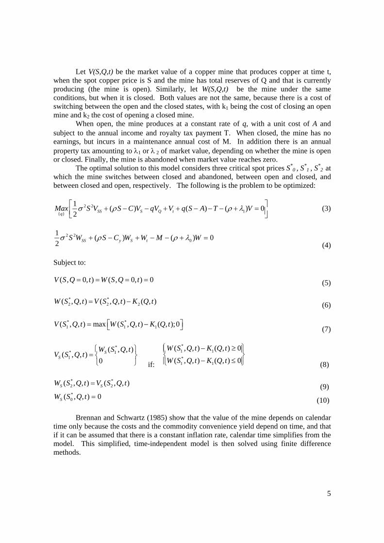
This procedure for finding the basis has the benefit of being simple, but may present numerical and performance problems with multidimensional models due to its high number of regressors. Figure 3 illustrates how the number of regressors increases with multi-dimensional problems as the order of the base is increased. To control for this high number of regressors, many times multidimensional problems are estimated using a low-order base, with the obvious loss of accuracy.

12

Number of Regressors as a function of the Order and Dimension of the problem

0

10

20

30

40

50

60

1 2 3 4 5

Order Polynomials

Num

ber o

f Reg

ress

ors 1 Dimension

2 Dimension

3 Dimension

4 Dimension

Figure 3 Number of regressors as a function of the dimension of the problem and the order of the base.

This procedure for specifying the base, having the advantage of being very simple, does not take advantage on the structure of the problem to be solved. Given that in most financial options optimal exercise depends on expected spot prices and volatilities, we propose using this knowledge on the determinants of option value for the base selection. Then, instead of using functions of all combinations of the state variables, we propose using powers of expected spot prices which should dramatically reduce model complexity, while providing an accurate computation of option value. So Eq. (27) becomes under our specification:

01

ˆ ˆ ˆ( ) ( )N

iN i

ig a a E S

=

= + ∑x (29)

where E(S) is the expected spot price under the risk-adjusted measure, i.e., the futures price. Using this reduced-base specification we can obtain similar valuation accuracy in a much simpler way, as will be seen in the next section. 3.3 Testing the reduced-base for valuing a three-factor European Option.

To test our reduced-base proposition we value an option that has a closed-form solution and compare the analytic solution to alternative implementations of the LS01 method. The example used is the pricing at time t of the option to extract and sale q pounds of copper in T. This is a European option (instead of an American one), but we include a three-factor model for the stochastic process of copper prices. Also, given that American options in their last exercise opportunity become in practice a European one, we can compare the expected continuation value function at the last exercise date obtained from the LS01 method with the analytic expression for a European option with T-t maturity.

Using the three-factor model shown earlier, we let ln( )t tx S= , then using Ito’s lemma to obtain the discrete-time form for simulating the state variables when 0t∆ → :

13

21 1 1 1

1 2 2

1 3 3

1 1 1 1 2 0 00 1 0 0 0 00 0 1 0 0

t t

t t

t t

x xy y t t

a a

σ σ εκ σ ε

υ υ ν σ ε

−

−

−

⎡ ⎤⎛ ⎞− −⎛ ⎞ ⎛ ⎞⎛ ⎞ ⎛ ⎞ ⎛ ⎞⎢ ⎥⎜ ⎟⎜ ⎟ ⎜ ⎟⎜ ⎟ ⎜ ⎟ ⎜ ⎟= − + ∆ + ∆⎢ ⎥⎜ ⎟⎜ ⎟ ⎜ ⎟⎜ ⎟ ⎜ ⎟ ⎜ ⎟

⎜ ⎟ ⎜ ⎟⎜ ⎟ ⎜ ⎟ ⎜ ⎟⎢ ⎥⎜ ⎟−⎝ ⎠ ⎝ ⎠⎝ ⎠ ⎝ ⎠ ⎝ ⎠⎝ ⎠⎣ ⎦

B (30)

where B is the Cholesky decomposition of the instantaneous correlation matrix in three dimensions:

21 1

31 2 3

1 0 00B ρ

ρ

⎛ ⎞⎜ ⎟= Ρ⎜ ⎟⎜ ⎟Ρ Ρ⎝ ⎠

21 211 ρΡ = − 23 21 31

21

ρ ρ ρ−Ρ =

Ρ

231 2

31

1 ρ− − ΡΡ =

Ρ (31)

1 2 3, , (0,1)Nε ε ε ∼ The closed-form value for the European option is:

1ln( ) ln( ) ( ) ( )21 2( , , , , ) N( ) N( )t T t TE S Var S r T t r T t

t t tC S y t T q e d K d eυ+ − − − −⎡ ⎤

= −⎢ ⎥⎣ ⎦ (32)

where N is the cumulative normal distribution,

1ln( ) ln( ) ln( )

ln( )t T t T

t T

E S Var S KdVar S+ −

=;

2ln( ) ln( )

ln( )t T

t T

E S KdVar S

−=

(33)

( ) ( )

2321 1

( ) ( ) 2232

(ln( )) (1 e ) / (1 e ) /1( )( )2

(e 1) (e 1)( ) /

T t a T tt T t t t

T t a T t

E S x y a

T ta

a a

κ

κ

κ νλλν λ σ

κλ ν λκ

− − − −

− − − −

= − − + −

+ + − − − −

+ − + − − (34)

14

22 ( ) 2 ( )21 2

2( ) 2 ( )3

2

( )12 1 2

( )13 1 3

23 2

2 1ln( ) ( ) ( ) (1 e ) (1 e )2

2 1( ) (1 e ) (1 e )2

2 1( ) (1 e )

2 1( ) (1 e )

2

T t T tt T

a T t a T t

T t

a T t

Var S T t T t

T ta a a

T t

T ta a

κ κ

κ

σσκ κ κ

σ

ρ σ σκ κ

ρ σ σ

ρ σ

− − − −

− − − −

− −

− −

⎡ ⎤= − + − − − + −⎢ ⎥⎣ ⎦

⎡ ⎤+ − − − + −⎢ ⎥⎣ ⎦⎡ ⎤− − − −⎢ ⎥⎣ ⎦⎡ ⎤+ − − −⎢ ⎥⎣ ⎦

− ( ) ( ) ( )( )3 1 1 1( ) (1 e ) (1 e ) (1 e )T t a T t a T tT ta a a

κ κσκ κ κ

− − − − − + −⎡ ⎤− − − − − + −⎢ ⎥+⎣ ⎦

(35)

Once we have a closed-form solution to our problem we compare two different

specifications for the regression base: first the original recommendations and then our reduced-base implementation.

We did several numerical implementations of LS01 method using Legendre, Laguerre, Hermite, Chebyshev polynomials, all of them converging to the known analytic solution in a similar way. We then implemented our reduced-base proposition for different number of regression terms. Figure 4 compares the RMSE of both approaches as a function of the number of regressors. It can be seen that even though introducing more regressors to the base lowers the RMSE for both approaches, using our reduced-base proposition requires a much lower number of regressors to achieve a given level of the RMSE.

Regression Adjustment Level to Analytic in Chebyshev Polynomials and Reduced Form Proposed

0%

1%

2%

3%

4%

5%

6%

7%

8%

9%

0 10 20 30 40 50 60Number of Regressors - Increasing order

RM

SE %

Chebyshev

Reduced Form

Figure 4 Regression RMSE as a function of the number of regressors for Chebyshev Polynomials and the reduced-base form.

15

4. Model Implementation and Results In this section we show how to implement the Longstaff and Schwartz (2001) method to solve the extended Brennan and Schwartz (1985) model. The reduced-base implementation proposed earlier in this paper is used to solve this real option model under prices that follow the Cortazar and Schwartz (2003) three-factor commodity price model, calibrated for copper.

Then, we restrict the commodity price model to match the one-factor model used in the Brennan and Schwartz (1985) paper and compare their results using finite difference methods with those from our simulation method. Finally, we present our results for the real option model with the three-factor price process.

4.1 Model Implementation. In a previous section we described the extended Brennan and Schwartz (1985) model including the options to abandon a mine, to close an open mine and to open a closed mine. Also we described the computer-based simulation approach that will be used for solving the model. Figure 5 may be useful to understand the nature of the problem by describing all possible states during the simulation. It can be seen that as time evolves from 0 to T, the state variables that describe the dynamics of copper prices, [ , , ]

t t t tS yω ω ω ωυ=x , evolve

following different paths. At any point in time, and for any value of the price state variables, the mine may have any amount of copper reserves between zero and the initial reserves Qmax. In addition, the mine at that point may be open or closed with market values

( , )t

V Qωx or ( , )t

W Qωx , respectively.

Figure 5 State-space representation of the extended Brennan and Schwartz (1985) model extended with a multi-factor price process

T

0X ( )t ωX

t

( )T ωX

OPE

N

CLO

SED

Qmax

Qmin

Reserve

s

OPE

N

CLO

SED

Stat

e Var

iabl

es

16

For every state of the system and operating policy, there is an associated cash flow for the firm. For example, when the mine is open and the operating policy is to remain open during t∆ years producing q*, the cash flow, CF, is: ( , *) * ( )

t tCF S q q t S A Taxω ω= ∆ − − (36)

Recall that for any price model, the spot price depends on the state variables x, i.e. ( )

t tS fω ω= x . In particular, for the three-factor CS01 model used in this paper, we have:

( ) 't t t

S fω ω ω= =x h x with [ ]' 1 0 0=h (37)

Also, as noted previously, the mine may be open, closed or abandoned, and may switch from one operating state to another incurring in fixed costs.

Figure 6 summarizes the cash flows of an open mine which will either remain open, be closed or abandoned during time t. Figure 7 shows the same information, but for a closed mine.

Figure 6. Cash flows and Value of an Open Mine as a function of Operating Policy

Figure 7 Cash flows and Value of an Open Mine as a function of operating policy

Open Mine

( , )t

V Qωx

Abandon

Close

Continue Open

Operating Policy Cash Flow at t Value at t+1

1( , )

tV Q q tω +

− ∆x

1( , )

tW Qω +

x

0V W= =

( , *)t

CF S qω

1K M t− ∆

0

Open Mine

( , )t

V Qωx

Abandon

Close

Continue Open

Operating Policy Cash Flow at t Value at t+1

1( , )

tV Q q tω +

− ∆x

1( , )

tW Qω +

x

0V W= =

( , *)t

CF S qω

1K M t− ∆

0

Closed Mine

( , )t

W Qωx

Abandon

Continue Closed

Open

Operating Policy Cash Flow at t Value at t+1

1( , )

tV Q q tω +

− ∆x

1( , )

tW Qω +

x

0V W= =

2( , *)t

CF S q Kω −

M t− ∆

0

17

As described in a previous section, after simulating all price paths from time zero to

time T, the method requires making optimal decisions starting at time T and then working backwards until the initial time zero is reached. The optimal decision at each point is taken by maximizing market value among all available decision alternatives. At time T, given that the concession ends, the value of both the open and the closed mine is zero: ( , ) ( , ) 0 ,

T TV Q W Q Qω ω ω= = ∀ ∀x x (38)

Then, at t T t= − ∆ there is no time left to change the operating policy so there is no need to estimate an expected continuation value. So the market values are:

1( )( , ) ( ( , *);0)T t T t

r tV Q Max CF S q e λω ω−∆ −∆

− + ∆=x Q∀ (39) 0( )

2( , ) ( ( , *) ;0)T t T t

r tW Q Max CF S q K e λω ω−∆ −∆

− + ∆= −x Q∀ (40) Then, at 2t T t= − ∆ we must estimate the expected continuation value. We regress mine value on a linear combination of functional forms of the state variables L(X), for each inventory level Q:

2 , , 2 , , 2( , ) ( , ) ( )T t T t T t V Q T t W Q T tV Q W Q L a a e

−∆ −∆ − ∆ − ∆ − ∆⎡ ⎤ ⎡ ⎤= +⎣ ⎦⎣ ⎦X X X (41)

Once the optimal coefficients are found we can estimate expected continuation values for any mine:

, , 2 , , 2 , , 2 , , 2ˆ ˆ ˆ ˆ( )V Q T t W Q T t t V Q T t W Q T ta a− ∆ − ∆ − ∆ − ∆

⎡ ⎤ ⎡ ⎤= ⎣ ⎦⎣ ⎦G G L X (42)

Thus, the expected continuation value at time 2t T t= − ∆ , as a function of the price state variables x, may be computed. For example, the value of an open mine with Q units of resources, conditional on keeping the mine open would be:

, , 2 , , 21

ˆ ˆ( ) ( )M

V Q T t V Q T t jj

g a L− ∆ − ∆=

= ∑x x (43)

Given that we can compute the expected continuation value for all mines (open or closed and with any amount of reserves left), we are now able to obtain the optimal operating decisions by maximizing current cash flows plus the present value of expected continuation values. For example, when the mine is open there are three operating alternatives available: to continue open, to close down operations, or to abandon the mine. Adding current cash flows to discounted expected continuation values for each of the three alternatives, the decision maker may choose which is the best course of action.

Figure 8 shows, for each of the three alternatives, the expected present value (at time t), the optimal decision should this expected present value be the maximum among the alternatives, and the final value at time t using actual realizations of the price simulation (instead of expected values to avoid known biases) at time t+1. Figure 9 shows the same information, but if the mine is initially closed.

18

Open MineExpected and Realized Value

Abandon

Close

Continue Open

Optimal DecisionExpected Value Realized Value

, ,ˆ( , *) ( )t tV Q q t tCF q gω ω− ∆+x x

1 , 1,ˆ ( )tW Q tK M t g ω−− − ∆ + x

0

1

1

( )( , ) ( , *) ( , )t t t

r tV Q CF q V Q q t e λω ω ω +

− + ∆= + − ∆x x x

0

1

( )1( , ) ( , )

t t

r tV Q K M t W Q e λω ω +

− + ∆= − − ∆ +x x

( , ) 0t

V Qω =x

Figure 8 Expected and Realized Value of an Open Mine as a function of Operating Policy

Closed MineExpected and Realized Value

Abandon

Continue Closed

Open

Optimal DecisionExpected Value Realized Value

0

2 , ,ˆ( , *) ( )t tV Q q t tK CF q gω ω− ∆− + +x x

, 1,ˆ ( )tW Q tM t g ω−− ∆ + x

( , ) 0t

W Qω =x

0

1

( )( , ) ( , )t t

r tW Q M t W Q e λω ω +

− + ∆= − ∆ +x x

1

1

( )2( , , ) ( , *) ( , )

t t t

r tW Q t K CF q V Q q t e λω ω ω +

− + ∆= − + + − ∆x x x

Figure 9 Expected and Realized Value of a Closed Mine as a function of Operating Policy.

19

This procedure is repeated from 2t T t= − ∆ until 2t t= ∆ . At t t= ∆ mine values are averaged over all price paths to provide an initial estimate of the expected continuation value for the mine:

1

0

( ), , 0

1

1ˆ ( ) ( , )s

r tV Q q t tg V Q q t e

sλ

ω ωω

− + ∆− ∆ =

=

= − ∆∑x x (44)

0

0

( ), , 0

1

1ˆ ( ) ( , )S

r tW Q tg W Q e

Sλ

ω ωω

− + ∆=

=

= ∑x x (45)

Figures 10 and 11 show the initial mine values depending on the initial status and operating policy of the mine

Figure 10 Open Mine values as a function of the initial operation decision. Figures 11 Closed Mine values as a function of the initial operation decision.

Finally, to determine the optimal operating policy, described by the critical values for the state variables over or under which it is optimal to switch between mine states (abandoned, closed and open) the method must find the critical state variables, xc

which equate expected present values for different operating decisions.

Open Mine Value

Abandon

Close

Continue Open 1

0 0

( ), , 0ˆ( , ) ( , *) ( )

t

r tV Q q t tV Q CF q g e λ

ω ω ω− + ∆

− ∆ == +x x x

0

0 0

( )1 , , 0ˆ( , ) ( ) r t

W Q tV Q K M t g e λω ω

− + ∆== − − ∆ +x x

0( , ) 0V Qω =x

Closed Mine Value

Abandon

Continue Closed

Open 1

0 0 0

( )2 , , 0ˆ( , ) ( , *) ( ) r t

V Q q t tW Q K CF q g e λω ω ω

− + ∆− ∆ == − + +x x x

0

0 0

( ), , 0ˆ( , ) ( ) r t

W Q tW Q M t g e λω ω

− + ∆== − ∆ +x x

0( , ) 0W Qω =x

20

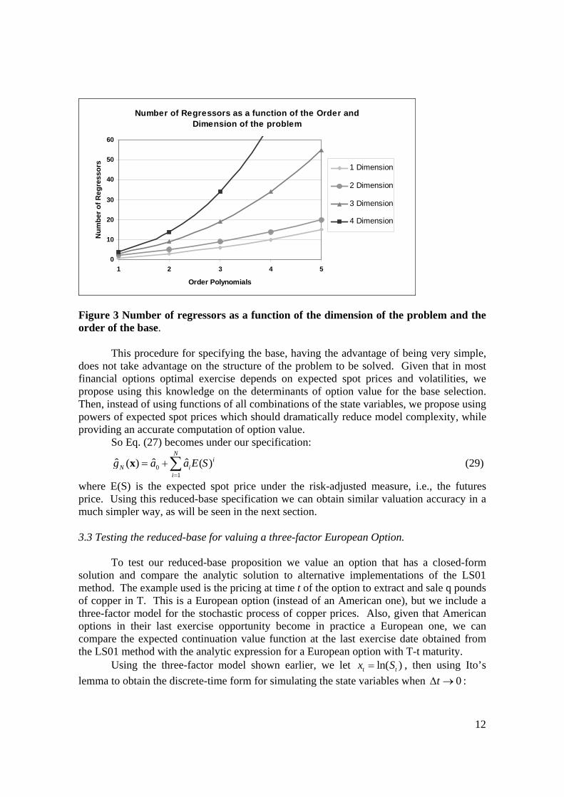
Figure 12 shows how to find the critical state variables to close an open mine, to open a closed mine, or to abandon from an open or from a closed mine. Figure 12 Conditions to determine critical state variables xc for switching mine operating policy 4.2 Results for the original Brennan and Schwartz (1985) model. To validate the proposed procedure, in this section we solve the Brennan and Schwartz (1985) real options model that was originally solved using traditional finite difference methods. Recall that the main difference between this model and its extension, which will be solved in the following section, is the price process with one or three risk factors, respectively. A simple way of validating our method is to see the one-factor price process as a particular case of the more general three-factor process. In this way by restricting certain parameter values we can perform a better test on the algorithm by using the same computer program to solve both models. Table 2 shows how the Cortazar and Schwartz (2003) three factor model may be restricted to behave as the one-factor model used in Brennan and Schwartz (1985):

Optimal Policy

Open to Abandon

Closed to Open

Open to Closed

Equilibrium Condition

Closed to Abandon

, , 1 , 1,ˆ ˆ( , *) ( ) ( )c c cV Q q t t W Q tCF q g K M t g− ∆ −+ = − − ∆ +x x x

, 1, 2 , ,ˆ ˆ( ) ( , *) ( )c c cW Q t V Q q t tM t g K CF q g− − ∆− ∆ + = − + +x x x

, ,ˆ( , *) ( ) 0c cV Q q t tCF q g − ∆+ =x x

, 1,ˆ ( ) 0cW Q tM t g −− ∆ + =x

21

Cortazar-Schwartz Model Parameters

Equivalence to Brennan-Schwartz

1λ 0 0 1( )y rυ δ λ− − − =

2λ 0≈

3λ 0≈

a 1

κ 1

ν 0≈

1σ σ

2σ 0≈

3σ 0≈

12ρ 0≈

23ρ 0≈

13ρ 0≈

oy 2 /λ κ

oυ 3 / aν λ−

Table 2 Restrictions on the parameters of the Cortazar and Schwartz (2003) model which induce a one-factor price process similar to Brennan and Schwartz (1985).

The proposed computer-based simulation program was run for 50000 price paths,

assuming a concession that lasted for 50 years (the original model assumes an infinite concession), and there are three opportunities/year to switch between operating states.

Table 3 compares the finite difference values reported in Brennan and Schwartz (1985) with those obtained using the above simulation procedure. It can be seen that the simulation method converges very nicely to the known solution.

22

Mine Value Finite difference method

reported in Brennan-Schwartz (1985)

Mine Value Simulation method

Spot Price (US$/lb.)

Open Closed Open Closed

0.4 4.15 4.35 4.2 4.4

0.5 7.95 8.11 7.93 8.12

0.6 12.52 12.49 12.51 12.49

0.7 17.56 17.38 17.51 17.31

0.8 22.88 22.68 22.8 22.6

0.9 28.38 28.18 28.29 28.09

1.0 34.01 33.81 33.89 33.69

Table 3 Open and Closed Mine Value as a function of spot price.

0,00

0,10

0,20

0,30

0,40

0,50

0,60

0,70

0,80

0,90

102030405060708090100110120130140150

Reserves

Crit

ic P

rice

(US$

)

open close abandon

Optimal Policy Simulation Method

0,00

0,10

0,20

0,30

0,40

0,50

0,60

0,70

0,80

0,90

102030405060708090100110120130140150

Reserves

Crit

ic P

rice

(US$

)

open close abandon

Optimal Policy Simulation Method

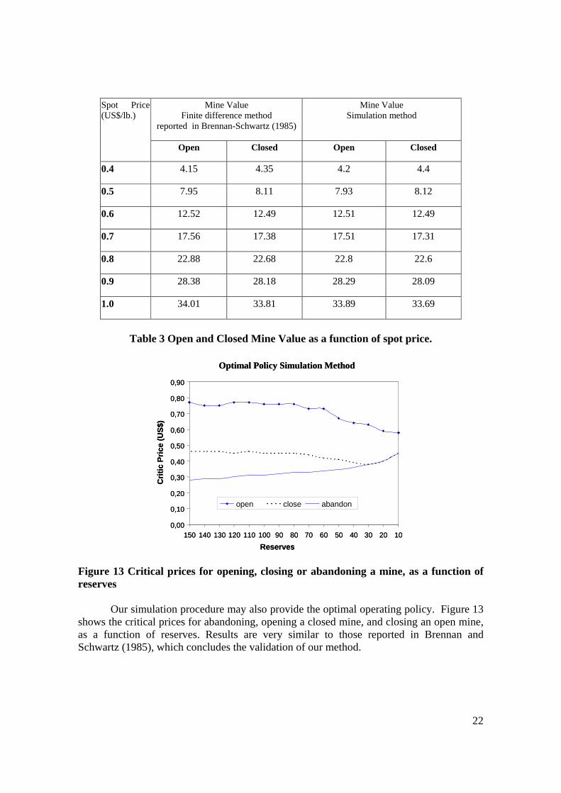
Figure 13 Critical prices for opening, closing or abandoning a mine, as a function of reserves

Our simulation procedure may also provide the optimal operating policy. Figure 13

shows the critical prices for abandoning, opening a closed mine, and closing an open mine, as a function of reserves. Results are very similar to those reported in Brennan and Schwartz (1985), which concludes the validation of our method.

23

4.3 Results for the three-factor extension of the Brennan and Schwartz (1985) model.

We now report the solution to the Brennan and Schwartz (1985) model extended to include the Cortazar and Schwartz (2003) three-factor commodity price model. The used parameter values are those estimated from all copper futures prices traded at NYMEX between 1991 and 1998 and reported in section 2.3.

The computer-based simulation is run for 10,000 price paths, assuming a 30 year concession horizon, and three opportunities to switch operation mine state per year. To value the mine for a particular date, say January the 14th, 1999, we must first determine the values of the state variables corresponding to that date, which we report in Table 4.

State Variable Value

oS 0,65

oy 0,465

oυ 0,417

Table 4 Values of the state variables for January the 14th, 1999

We now run the simulation and the procedure described in 4.1 obtaining for that

date a value for the open mine of MMUS$ 16,75, and for the closed mine of MMUS$ 16,68. To explore how mine value changes according to daily variations in price conditions, we solve for the value of the mine for a 5 year time span, at each date between January 1999 and December, 2003. Results are reported in Figure 14.

Daily Values of the Extended Brennan y Schwartz (1985) Open Mine

1214161820222426283032

01-99 08-99 02-00 09-00 03-01 10-01 05-02 11-02 06-03 12-03

Dates

MM

US$

Figure 14 Daily values of the extended Brennan and Schwartz (1985) open mine according to historical copper pricing conditions from January 1999-December 2003

24

It is interesting to note that mine value exhibits mean reversion. Even though it is

well known that copper prices do exhibit mean reversion, given that a mine produces copper during a long time span it could be thought that current spot prices would not affect too much mine values, so this value would not display mean reversion. Figure 14 shows this is not the case.

To make comparative static analysis on how mine value changes with variations in the spot price, or in any individual state variable or parameter value, is rather straightforward. For example, Figure 15 shows how mine value increases with copper spot prices. Also it is interesting to note that mine values are convex, as with all options, because as value approaches zero the mine increases the probability of abandonment. Finally, the same figure compares mine value computed with the real option model to a simple net present value calculation which does not recognize operating flexibilities to abandon or close operations. It can be seen that when spot prices are lower, option values are greater and these two valuation methodologies diverge by the most. By the same token, when prices are high, flexibilities are not too valuable and both valuations converge.

Mine Value Extended Brennan Schwartz (1985): y = 0.01, v = -0.1

-15

-10

-5

0

5

10

15

20

25

0.4 0.5 0.6 0.7 0.8

Spot Copper Price (US$)

MM

US$

NPV Open Mine ROV Closed Mine ROV

Figure 15 Mine Value using ROV and NPV as a function of spot price

We can repeat the comparative static analysis for any of the state variables. For example, in Figure 16 we compare Real Option and traditional NPV values as a function of the short term price deviations, y. We assume a rather low initial spot price of only US$0.4. Recall that our three-factor price model assumes that short-term price variations, y, mean revert to zero. Thus, if at any point in time y exhibits a high positive value, future prices are expected to be much lower than current ones, and given our low initial spot price assumption, mine value should basically be explained by its option value. This can be seen

25

in Figure 16 where for large values of y the NPV shows a negative value, while the ROV value is slightly positive.

Mine Value Extended Brennan Schwartz (1985):S = 0.4, v = 0.3

-15

-10

-5

0

5

10

-0.4 -0.2 0 0.2 0.4 0.6 0.8 1

Short Term Price Deviations (y)

MM

US$

NPV Closed Mine ROV Open Mine ROV

Figure 16 Mine Value using ROV and NPV as a function of short-term price deviations

Comparative static analysis can also be performed on optimal policy results. For example Figure 17 shows how critical spot prices to open a closed mine depend both on price conditions, in this case the value of the short term price deviations y, and on the state of the mine, represented by the reserves left for extraction.

Optimal Opening Prices as a function of Short Term Deviations (y)

0.4

0.5

0.6

0.7

0.8

0.9

1

5305580105130

Mine Reserves MM tons

Crit

ic P

rice

US$

Opening y= -0.15 Opening y= 0.15 Opening y= 0.5

Figure 17 Critical spot prices for opening a closed mine as a function of short term price deviations and mine reserves

26

Sometimes optimal policy evolves in a non-monotonic way with the state of the mine. For example in Figure 18 where as reserves are lower, critical closing prices first decline to later sharply increase.

Optimal Closing Prices as a function of Short Term Deviations (y)

0.3

0.35

0.4

0.45

0.5

525456585105125145

Mine Reserves MM tons

Crit

ic P

rice

US$

Close y= -0.15 Close y= 0.15 Close y= 0.5

Figure 18 Critical spot prices for closing an open mine as a function of short term price deviations and mine reserves 5. Conclusions

Real options valuation (ROV) is an emerging paradigm that provides helpful insights both for valuing and for managing real assets. It provides more precise quantifications on the value of available strategic and operational flexibilities than traditional discounted cash flow techniques. Despite its potential, the ROV approach has not yet made a strong inroad in corporate decision-making due to several reasons, one of which is the requirement to keep models too simple to obtain solutions within a reasonable amount of effort. In this paper we show how it is possible to solve very complex multidimensional American options resorting to new computer-based simulation procedures. We show how to lower complexity by using a reduced-base implementation of the procedure and we validate our proposition solving a multidimensional option with known analytical solution. We then extend a known real option model proposed by Brennan and Schwartz (1985) and solve it using the proposed methodology. Results on different comparative static analysis are provided. This paper makes the case why these new computer-based simulation methods have the potential of expanding significantly the use of the ROV approach without having to compromise rigorous modeling for solving requirements.

27

REFERENCES Andersen L. A Simple Approach to the pricing of bermudian Swaptions in the Multi-Factor Libor market Model. Journal of Computational Finance 3: 5-32, 2000. Barraquand J, Martineau D. Numerical Valuation of High Dimensional Multivariate American Securities. Journal of Financial and Quantitative Analysis 30 (3): 301-320, 1995. Bernardo A, Chowdry B. Resources, Real Options and Corporate Strategy. Jounal of Finance 63: 211-234, 2002. Black F, Scholes M. The pricing of options and corporate liabilities. Journal of Political Economy 81: 637-654, 1973. Bossaerts P. Simulation Estimators of Early Optimal Exercise: Graduate School of Industrial Administration, Carnegie Melon University, 1988. Brennan MJ, Schwartz ES. Evaluating natural resources investments. Journal of Business 58 (2): 135-157, 1985. Brennan MJ, Trigeorgis L. Project flexibility, agency, and competition: Oxford University Press, 2000. Broadie M, Glasserman P. Pricing American-Style Securities using simulation. Journal of Economics Dynamics and Control 21 (8): 1323-1352, 1997. Casassus J, Collin-Dufresne P. 'Maximal' convenience yield model implied by commodity futures. Jounal of Finance forthcoming, 2004. Clement E, Lamberton D, Protter P. An analysis of a least squares regression method for American option pricing. Finance and Stochastics 6 (4): 449-471, 2002. Cortazar G, Casassus J. Optimal timing of a mine expansion: Implementing a real options model. The Quarterly Review of Economics and Finance 38: 755-769, 1998. Cortazar G, Schwartz ES. A compound option model of production and intermediate investement. Journal of Business 66 (4): 517-540, 1993. Cortazar G, Schwartz ES. Implementing a real option model for valuing an undeveloped oil field. International Transactions in Operational Research 4 (2): 125-137, 1997. Cortazar G, Schwartz ES. Implementing a stochastic model for oil futures prices. Energy Economics 25 (215-238), 2003. Decamps J, Mariotti T, Villeneuve S. Investment timing under incomplete infor-mation. Stockholm: European Economic Association Annual Congress, 2003.

28

Dixit A. Entry and Exit Decisions under Uncertainty. Journal of Political Economy 97: 620-638, 1989. Dixit A, Pindyck R. Investment under Uncertainty: Princeton University Press, 1994. Ekern S. An Option Pricing Approach to Evaluating Petroleum Projects. Energy Economics 10: 91-99, 1988. Gibson R, Schwartz ES. Stochastic convenience yield and the pricing of oil contingent claims. The Journal of Finance 45 (3): 959-976, 1990. Haugh M, Kogan L. Approximating Pricing and Exercising of High-Dimensional American Options: A Duality Approach: MIT, 2001. He H, Pindyck R. Investment in Flexible Production Capacity. Journal of Economics Dynamics and Control 16: 575-599, 1992. Hsu J, Schwartz ES. A Model of R&D Valuation and the Design of Research Incentives. Los Angeles: Andreson School, UCLA, 2003. Kulatilaka N. Operating Flexibilities in Capital Budgeting: Substitutability and Complementarity in Real Options. In: Trigeorgis L, ed. Real Options in Capital Investments: New Contributions. New York: Praeger, 1995. Lambrecht B, Perraudin W. Real Options and Preemption Under Incomplete Information. Journal of Economic Dynamics and Control 27 (4): 619-643, 2003. Laughton DG, Jacoby HD. The effects of reversion on commodity projects of different length. In: Trigeorgis L, ed. Real options in capital investments: Models, strategies, and applications. Westport: Praeger Publisher, 1995. Laughton DG, Jacoby HD. Reversion, timing options, and long-term decision-making. Financial Management 22 (3): 225-240, 1993. Lehman J. Valuing Oilfield Investments Using Option Pricing Theory. SPE Hydrocarbon Economics and Evaluation Symposium, Proceedings: 125-136, 1989. Longstaff FA, Schwartz ES. Valuing american options by simulation: A simple least -squares approach. The Review of Financial Studies 14 (1): 113-147, 2001. Majd S, Pindyck R. The Learning Curve and Optimal Production under Uncertainty. Rand Journal of Economics 29: 1110-1148, 1989. Majd S, Pindyck R. Time to Build, Option Value, and Investmnent Decisions. Journal of Financial Economics (18): 7-27, 1987. McDonald R, Siegel D. The value of waiting to invest. Quarterly Journal of Economics 101: 707-727, 1986.

29

Miltersen KR, Schwartz ES. R&D Investments with Competitive Interactions: NBER, 2003. Moreno M, Navas J. On the Robustness of Least-Squares Monte Carlo (LSM) for Pricing American Derivatives. Review of Derivatives Research (Forthcoming):, 2003. Murto P, Nasakkala E, Keppo J. Timing of Investments in Oligopoly Under Uncertainty: a Framework for Numerical Analysis. European Journal of Operations Research 157 (2): 486-500, 2004. Paddock J, Siegel D, Smith J. Option Valuation of Claims on Physical Assets: The Case of Offshore Petroleum Leases. Quarterly Journal of Economics 103 (3): 479-508, 1988. Pindyck R. Investment of Uncertain Cost. Journal of Financial Economics (34): 53-76, 1993. Raymar S, Zwecher M. A Monte Carlo valuation of American Call Options on the maximum of several stocks. Journal of Derivatives 5 (1 (Fall)): 7-23, 1997. Schwartz ES. The stochastic behaviour of commodity prices: Implications for valuation and hedging. The Journal of Finance 52 (3): 923-973, 1997. Schwartz ES, Smith JE. Short-term variations and long-term dynamics in commodity prices. Management Science 46: 893-911, 2000. Shackleton M, E. A, Tsekrekos, Wojakowski. Strategic Entry and Market Leadership in a Two-Player Real Option Game. Journal of Banking and Finance 28 (1): 19-201, 2004. Smith J, McCardle K. Options in the Real World: Lessons Learned in Evaluating Oil and Gas Investments. Operations Research 47: 1-15, 1999. Smith J, McCardle K. Valuing Oil Properties: Integrating Option Pricing and Decision Analysis Approaches. Operations Research 46: 198-217, 1998. Sørensen C. Modeling seasonality in agricultural commodity futures. Journal of Futures Markets 22: 393-426, 2002. Stentoft L. Assesing the Least Squares Monte-Carlo Approach to American Option Valuation. Review of Derivatives Research 7 (3): 129-168, 2004. Stentoft L. Assesing the Least Squares Monte-Carlo Approach to American Option Valuation: University of Aarhus, 2001. Tilley JA. Valuing American Options in a Path Simulation Model. Transactions of the Society of Ancuariess (45): 42-56, 1993.

30

Trigeorgis L. Evaluating leases with complex operating options. European Journal of Operations Research 91: 69-86, 1996. Trigeorgis L. The Nature of Option Interactions and the Valuation of Investments with Multiple Real Options. Journal of Financial and Quantitative Analysis: 1-20, 1993. Trigeorgis L. A real options application in natural resource investment. Advances in Futures and Options Research 4: 153-164, 1990.