The valuation of compensation expense under SFAS - Aabri.com

Journal of Finance and Accountancy

The valuation of compensation,

The valuation of compensation expense under SFAS 123R using

option pricing theory

John Gardner University of New Orleans

Carl McGowan, Jr.

Norfolk State University

Stephan Smith Norfolk State University

ABSTRACT

This paper demonstrates the impact of changes in option pricing model variables used in the Black-Scholes Option Pricing Model [BSOPM] on the valuation of compensation expense SFAS 123R. We provide a brief discussion of SFAS 123 and of the BSOPM and a detailed discussion of spreadsheets and graphs that show the impact that changing the values of the input variables of BSOPM has on the value of call options. The results not only provide evidence of the sensitivity of compensation expense to assumptions of the model’s variable values but can provide board members, managers, accountants and accounting students with insights into option granting policies. Keywords: SFAS 123R, Compensation Expense, Black-Scholes Options



INTRODUCTION

A number of studies including Choudary, Rajgopal and Venkatachalam (2009) and Beams, Amoruso and Richardson (2005) have addressed the impact of Statement of Financial Accounting Standards No 123 Share Based Payments (SFAS 123R) on the financial statements of U.S. companies. While the impact of the adoption of FAS 123 on corporate earnings is certainly of concern to boards of directors, managers and shareholders, the impact and sensitivity of the assumptions made in the fair value valuation models to the value placed on compensation expense has received little attention in the literature. As stated in an article in Quist Valuation

News (V3(1): 5) regarding pricing options, “From a valuation perspective, many issues appear relatively straightforward. Yet, we find that many companies are missing the nuances of binomial models and closed-end models (e.g. Black-Scholes).”

The purpose of this paper is to provide readers with an understanding of the sensitivity the calculation of option expense has to the individual factors used in a valuation model. Board members, managers, accountants and accounting students, by being aware of the impact changes in factor values have on the option expense, can make better and more informed decisions on option granting policy. In this paper we use the Black-Scholes Option Pricing Model [BSOPM] in our analysis. The application of the model assumes an American option but can be applied to European or Bermudan options which set specific exercise dates.

ACCOUNTING FOR STOCK OPTIONS UNDER SFAS 123R

The impact of FAS 123R is especially significant since, for the first time, both publically traded and non-publically traded companies were affected. For thinly traded public companies and non-public companies the determination of share price and volatility can be difficult to determine. The Black-Scholes simulation model used in this paper, and available from the authors, can be useful to managers, boards and owners of these companies to better understand the impact changing model variables have on the value of options. As noted by Pratesi (2008), “Needless to say, there are many traps and considerations for privately held companies in developing and implementing a stock option or stock-based compensation plan”. “SFAS 123R addresses the accounting for transactions in which an entity exchanges its equity instruments for goods or services. The statement eliminates the ability to account for share-based compensation transactions under the intrinsic-value method utilizing APB Opinion No. 25, Accounting for Stock Issued to Employees, and generally requires that such transactions be accounted for using the fair-value method. The techniques and procedures involved in the pricing of compensatory stock options are not defined in SFAS.”1

The compensatory stock option plan is an established corporate compensation tool. The accounting for stock option plans is relatively straight forward. The cost of the compensation provided in the stock option plan is to be expensed over the periods that the option recipient performs the duties and tasks that are compensated for by the stock option. The basic concept is that the stock option is priced to encourage the growth and expansion of the company through the increase in value of the underlying stock. The SFAS does not require the estimate of this potential value but the development of an estimate of the value of the option at the time of the award and the recognition of the expense over the vesting period.

1 thecaq.aicpa.org/Resources/Accounting/Statement+of+Financial+Accounting+Standards+No. +123R+Resource.htm



DEFINITIONS

a. The Option Price or exercise price is the price the company’s stock can be purchased by

the recipient of the compensatory stock option under the terms of the option contract. b. The exercise date is the date the stock option must be used to purchase the underlying

stock c. The Fair Value Method value is unknown and the calculation of the FVM value is the

purpose of this paper. There are competing Fair Value methods, we will examine the most popular the Black-Scholes method.

d. The Grant Date is the date the option is issued and the date the accounting estimate is established by the issuing company.

e. The Vesting Period is the number of periods that the employee receiving the option must strive to advance the traded price of the companies stock so that the share price exceeds the option price and generates a reward.

f. Compensation Expense is the amount estimated at the time of the compensatory stock option award and is expensed over the vesting period.

g. Changes in the Fair Value of the options during the vesting period are reflected in the fiscal period the changes occur in and do no effect the previous expense allocations in prior periods.

THE BLACK-SCHOLES OPTION PRICING MODEL

A call option provides the purchaser of the call with the right to purchase shares of a stock from the seller of the option at a pre-determined price, the exercise price. The buyer of a call option anticipates that the price of the optioned stock will increase. In the event that circumstances unfold according to plan, the buyer of the call will make a profit when the stock price increases because the ending stock price will be greater than the exercise price.

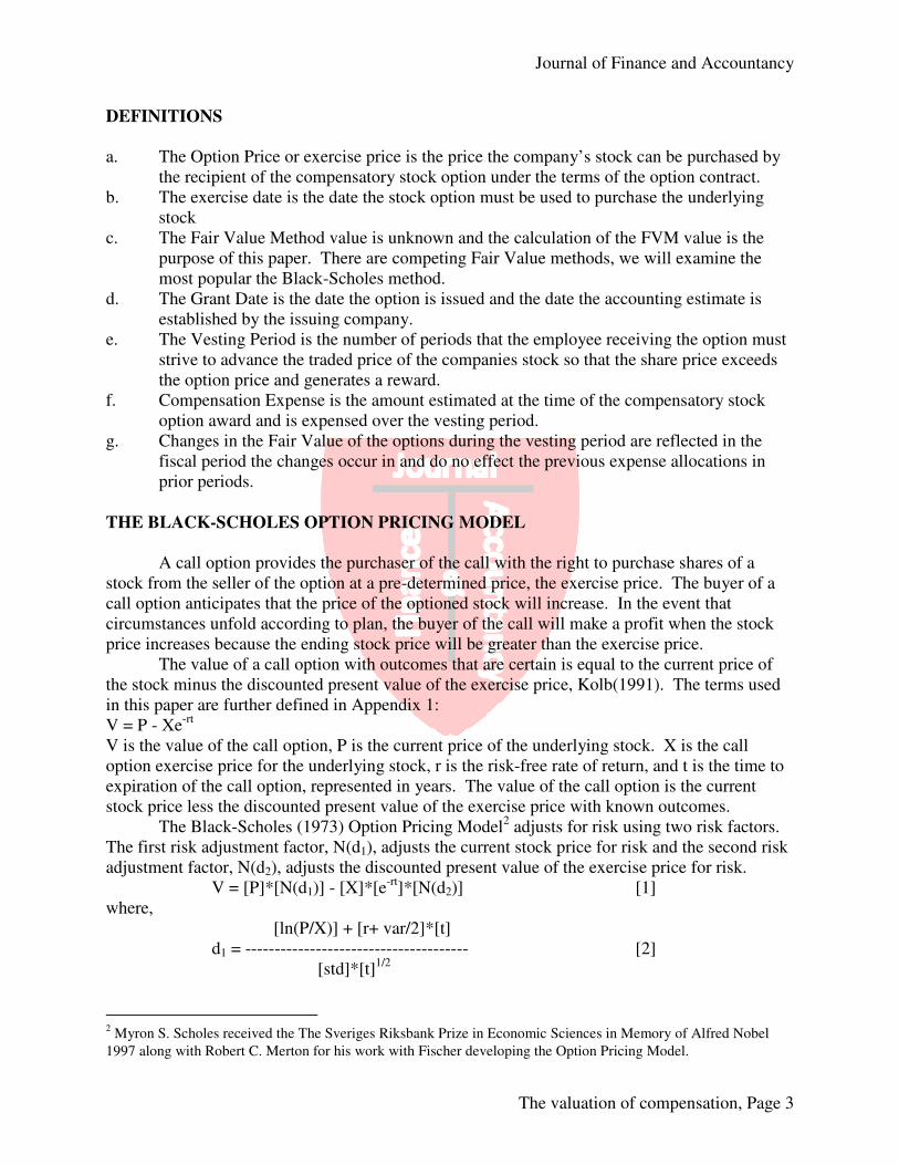
The value of a call option with outcomes that are certain is equal to the current price of the stock minus the discounted present value of the exercise price, Kolb(1991). The terms used in this paper are further defined in Appendix 1: V = P - Xe-rt V is the value of the call option, P is the current price of the underlying stock. X is the call option exercise price for the underlying stock, r is the risk-free rate of return, and t is the time to expiration of the call option, represented in years. The value of the call option is the current stock price less the discounted present value of the exercise price with known outcomes. The Black-Scholes (1973) Option Pricing Model2 adjusts for risk using two risk factors. The first risk adjustment factor, N(d1), adjusts the current stock price for risk and the second risk adjustment factor, N(d2), adjusts the discounted present value of the exercise price for risk. V = [P]*[N(d1)] - [X]*[e-rt]*[N(d2)] [1] where, [ln(P/X)] + [r+ var/2]*[t] d1 = -------------------------------------- [2] [std]*[t]1/2

2 Myron S. Scholes received the The Sveriges Riksbank Prize in Economic Sciences in Memory of Alfred Nobel

1997 along with Robert C. Merton for his work with Fischer developing the Option Pricing Model.



d2 = [d1] - [std]*[t]1/2

[ln(P/X)] + [r+ var/2]*[t] - [var]*[t] d2 = ------------------------------------------------- [3] [std]*[t]1/2 var is the instantaneous variance of the probability distribution of the underlying optioned stock, std is the standard deviation of the probability distribution of the underlying optioned stock, and ln is the natural logarithm function. N(:) represents the cumulative normal density function of the expression (:). N(:) is the probability that an outcome will be at least as great as the calculated value. Thus, using the BSOPM, the value of the call option can determined using 1. the price of the underlying optioned stock, 2. the instantaneous volatility of the optioned underlying stock, 3. the time to expiration of the call option, 4. the risk free rate of return, and 5. the exercise price for the underlying optioned stock. The value of the call option is positively related to variables 1 to 4 and negatively related to variable 5. For example, if the price of the underlying optioned stock increases, the value of the call option in increases. If the exercise price of the underlying optioned stock increases, the value of the call option in decrease. Calculating the Value of an Option

Table 1 contains the spreadsheet used to calculate the value of a call option using the Black-Scholes option pricing model. We use the Excel function normsdist(n) to determine the cumulative normal distribution values. This simplifies the spread sheet needed to do the calculations to determine the value of N(d1) and N(d2). Panel 1 of Table 1 contains the input values for each of the five input variables needed to calculate the value of an option: the price of the underlying common stock, P; the exercise price of the option, X; the risk-free rate of interest, r; the time to expiration, expressed as the proportion of a year, t; and the variance of the underlying stock return, var. Panel 2 of Table 1 contains the values of a call option on this stock. Panel 3 of Table 1 shows the values needed to calculate d1, d2, N(d1) and N(d2). The spreadsheet may be used to calculate the value of a call. In this example, the price of the underlying common stock is $50, the exercise price of the option is $60, the risk-free rate of interest is sixteen percent, the time to expiration of the option is one year, and the instantaneous variance of the stock returns is nine percent. Based on these numbers, the value of a call option on this stock is $5.48. The values needed to calculate the call value are [ln(P/X)], [r], [var/2], [t], [std], and [t]1/2. The computations are shown in detail in Appendix 2 and Appendix 3. Line 1 shows the value of ln(P/X) = ln(50/60) = -0.1823. Line 2 shows the value of [var/2] = (0.09/2) = 0.045. Line 3 show the value of [r + var/2]*[t] = [0.2050]. The numerator of d1 = ln[P/X] + [r + var/2]*[t] = [-0.1823 + 0.2050] =[0.0227]. Line 8 shows the value of [std]*[t]1/2 = [(0.09)1/2 * [(1.00)1/2] = [0.03000]. The value of d1 = [ln[P/X] + [r + var/2]*[t] / [-0.1823 + 0.2050] / [0.3000] = [0.0227]



/ [0.3000] = [0.0756]. The value of d2 = d1 – [std]*[t1/2] = [0.0756 – 0.3000] = -0.2244. The value of N(d1) = N(0.0756) = 0.5301 and the value of N(d2) = N(-0.02244) = 0.4112. The value of the call option is

V = [P]*[N(d1)] - [X]*[e-rt]*[N(d2)] V = [50]*[0.5301] – [60]*[0.8521]*[0.4112] V = 26.51 – 21.03 V = 5.48

Tables 1A to 1E show the calculations that show the impact of changes in each of the five input variables on the call option. By changing the input values, the decision maker sees the impact that changes in each of the variables have on the value of the call. However, the goal of this paper is to provide a more dynamic process than a single change and show the impact of changing each of the five independent variables over a range of values. Simulation Results

Appendices 1, 2 and 3 provide the definitions, worksheet and call option computation, respectively, used in the BSOPM calculations. Table 1 displays the values used in the BSOPM. We use this example as a basis for evaluating the effects in changes in each of the five variables (i.e. market price, exercise price, risk-free rate, expired time and variance) on the values of the call option. Changes in the Current Stock Price

Table 2A provides the BSOPM statistics on the value of call options when stock price changes from $50 to $59 while holding the other four variables constant. We see from the results that the 18 percent change in market price results in a 105 percent increase in the call value ($5.48 to $11.23). Put another way, the option price on average goes up $.57 for every $1.00 increase in stock price. Figure A provides a graph displaying the change in option values resulting from stock price changes. It is obvious from the graph that a change in stock price has a dramatic effect on the value of the option price and, of course, the greater the stock price the higher the probability the call will be exercised. Changes in the Exercise Price

Table 2B provides the BSOPM statistics on the value of call options with changes in the exercise price. The effect is opposite of stock price changes, with the call option decreasing 43.5 percent ($7.47 to $4.22) with a 16.4 percent ($55 to $64) increase in exercise price. In this case the option price, on average, goes down $.325 for every $1.00 increase in exercise price. Figure B provides a graph displaying the decrease in option price resulting from increases in the exercise price. This result is expected since the probability of a call option being exercised would decline as the exercise price increases. However, the value of the call option is less sensitive to the exercise price than the current market price. Changes in the Risk-Free Rate

Table 2C provides the BSOMP statistics of the effect on call options of changes in the risk-



free rate. The value of the call option changes increases 102 percent ($3.61 to $7.30) with a 300 percent (6 percent to 24 percent) increase in the risk-free rate. The option price, on average, increases $.205 for every percent increase in the risk free rate. Figure C provides a graph displaying the increase in option price with the increase in the risk free rate. Changes in the Time to Expiration

Table 2D shows the effect on option prices of changes in time to expiration. The effect on call option with the change in expiration is particularly pronounced with the call option value increasing $5.88 with every additional year in expiration time. Figure D displays the relationship graphically. This pronounced relationship shows the relative importance of the choice of expiration date in determining compensation. With the increase in expiration date the present value of the exercise price will decrease therefore increasing the value of the call option. In the case of European options which have a fixed expiration date, the option price will remain constant with other factors held constant. For the Bermudan option there will be separate increasing option price for each successive contractual option date. Changes in Variance of Return

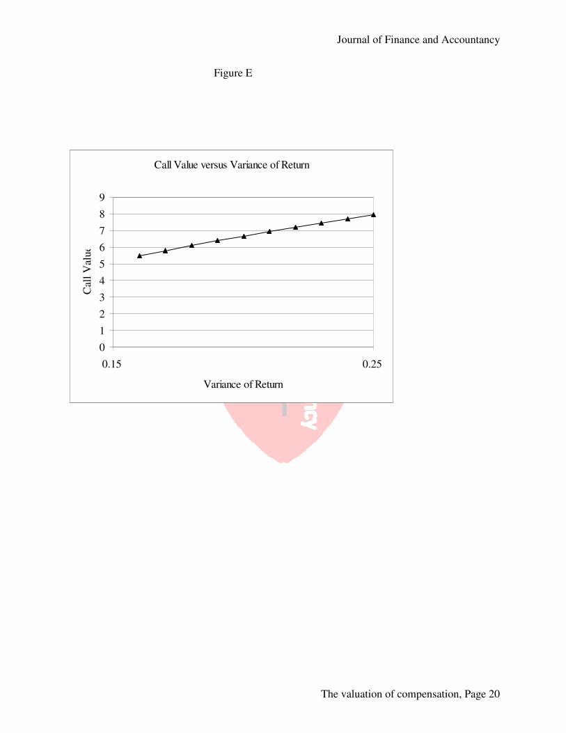
Table 2E shows the effect of changes in return variance on call option price. As the return variance changes from .09 to .18 (100 percent), the call value increases from $5.48 to $7.94 (44.7 percent). The result is a $.273 increase in the value of the call option for every 1 percent increase in variance of return. Figure E displays the relationship graphically. This analysis provides evidence that changes in the BSOPM model’s input variables have varying impact on the value of call options. The most dramatic effect on call option price results from changes in the expiration date, followed by changes in the current stock price. Changes in the risk-free rate and variance of returns are shown to have the least effect on call option value. These results are particularly interesting for non-public and thinly traded companies where the determination of stock price and variance of returns are often problematic. For board members, managers, accountants, and accounting students these results can provide a greater sensitivity to the importance of stewardship over the valuation and issuance of stock options. Summary and Conclusions

In this paper, we describe SFAS 123R and provide worksheet and spreadsheets (available from the authors) necessary to calculate the Black-Scholes option pricing values and provide evidence on the relative relationship between changes in the BSOPM variables and the value of call options. SFAS 123R requires auditors to confirm that stock options values provided by management are both consistent with the requirements SFAS 123R and are correctly computed using the Black-Scholes option pricing model. We provide examples and access to spreadsheets that can be used directly by board members, managers, accountants and accounting students to analyze the effect of changes in BSOPM variables on the pricing of put and call options.



REFERENCES

Beams, Joseph D., Amorous, Anthony J. and Richardson, Fredrick A. “Discretionary Reporting of

Stock Options by IPO Firms,” Accounting Horizons, Dec. 2005, Volume 19 Issue 4, pp. 223-236.

Black, Fischer and Myron Scholes. "The Pricing of Options and Corporate Liabilities," Journal of

Political Economy, (May-June 1973): pp. 637-654. Choudhary, Preeti, Rajgopal, Shivaram and Venkatachalam, Mohan,Accelerated “Vesting of

Employee Stock Options in Anticipation of FAS 123-R.” Journal of Accounting

Research, 2009, 47(1): pp. 105-146. Financial Accounting and Reporting, 2007 Edition Textbook, Becker CPA Review,

DeVry/Becker Educational Development Corp, pp. F7-22 to F7-23. Francis, Jack Clark. Investments: Analysis and Management, Fifth Edition, (McGraw-Hill: New

York), 1991. Kolb, Robert W. Options: An Introduction, (Kolb Publishing: Miami), 1991. Quist Valuation News, volume 3, number 1, 2006, page 4-5. Pratesi, Edward E. “Valuing Options While Running The Compliance Guantlet,” Soft Letter,

Vol. 24, No. 5, March 2008. thecaq.aicpa.org/Resources/Accounting/Statement+of+Financial+Accounting+Standards+No.,

+123R+Resource.htm www.fasb.org/pdf/fas123r.pdf



Appendix 1 Definitions P = the current price of the optioned stock X = the exercise price for the option e-rt = the present value interest factor for the exercise price r = the risk-free rate of interest var = the variance of the underlying stock = std2 std = the standard deviation of the underlying stock = the square root of the variance = var1/2 ln(:) = the natural logarithm operator ln(P/X) = the natural logarithm of the ratio of the current stock price and the exercise price N(:) = the normal distribution function = represents the area under the curve of a standard normal probability distribution = a positive value means that the area under the curve is greater than 0.50 = a negative value means that the area under the curve is less than 0.50 d1 = the risk adjustment factor for the current price = the number of standard deviations above or below the mean d2 = the risk adjustment factor for the exercise price = the number of standard deviations above or below the mean



Appendix 2 Work Sheet for the Options Examples [ln(P/X)] = ln[50/60] = -0.1823 [var/2] = [0.09/2] = 0.045 [r + var/2]*[t] = [0.2050] ln[P/X] + [r + var/2]*[t] = [-0.1823 + 0.2050] = [0.0227] [std]*[t]1/2 = [(0.09)1/2 * [(1.00)1/2] = [0.03000] d1 = [ln[P/X] + [r + var/2]*[t] / [std]*[t]1/2 = [-0.1823 + 0.2050] / [0.3000] = [0.0227] / [0.3000] = [0.0756] d2 = [d1] – [std]*[t1/2] = [0.0756 – 0.3000] = [-0.2244] N(d1) = N(0.0756) = [0.5301] N(d2) = N(-0.02244) = [0.4112.]

Appendix 3 Computing the Value of the Call Option Vcall = [P]*[N(d1)] - [X]*[e-rt]*[N(d2)] Vcall = [50]*[0.5301] – [60]*[0.8521]*[0.4112] Vcall = 26.51 – 21.03 Vcall = 5.48



Table 1 The Black-Scholes Option Pricing Model Numerical Method Calculation

Input Values Variable Value

Current price of underlying common stock P = 50.00

Exercise price of option X = 60.00

Risk-free rate of interest r = 0.16

Time to expiration t = 1.00

Variance of stock returns s^2 = 0.09

call value = 5.4813

Calculated Values:

ln(P/X) = -0.1823

[(s^2)/2] = 0.0450

[R+(s^2)/2] = 0.2050

[r+(s^2)/2]*[t] = 0.2050

ln(P/X) - [r+(s^2)/2]*[t] = 0.0227

s = 0.3000

t^(.5) = 1.0000

s*t^(.5) = 0.3000

e^(-rt) = 0.8521

d1 = 0.0756

d2 = -0.2244

N(d1)= 0.5301

N(d2)= 0.4112

Call value = 5.4813



Table 2A Call Valuation Current Stock Price

(1) (2) (3) (4) (5) (6) (7) (8) Current Exercise Risk-free Expire Instant Price Price Rate Time Variance

(P) (X) (r) (t) (s^2) ln(P/X) (s^2)/2 s*(t^0.5)

50.00 60.00 0.16 1.00 0.09 -0.1823 0.0450 0.3000

51.00 60.00 0.16 1.00 0.09 -0.1625 0.0450 0.3000

52.00 60.00 0.16 1.00 0.09 -0.1431 0.0450 0.3000

53.00 60.00 0.16 1.00 0.09 -0.1241 0.0450 0.3000

54.00 60.00 0.16 1.00 0.09 -0.1054 0.0450 0.3000

55.00 60.00 0.16 1.00 0.09 -0.0870 0.0450 0.3000

56.00 60.00 0.16 1.00 0.09 -0.0690 0.0450 0.3000

57.00 60.00 0.16 1.00 0.09 -0.0513 0.0450 0.3000

58.00 60.00 0.16 1.00 0.09 -0.0339 0.0450 0.3000

59.00 60.00 0.16 1.00 0.09 -0.0168 0.0450 0.3000

(9) (10) (11) (12) (13) (14) Call e^(-rt) d1 d2 N(d2) N(d1) Value

0.8521 0.0756 -0.2244 0.4112 0.5301 5.48

0.8521 0.1416 -0.1584 0.4371 0.5563 6.02

0.8521 0.2063 -0.0937 0.4627 0.5817 6.59

0.8521 0.2698 -0.0302 0.4880 0.6064 7.19

0.8521 0.3321 0.0321 0.5128 0.6301 7.81

0.8521 0.3933 0.0933 0.5372 0.6529 8.45

0.8521 0.4534 0.1534 0.5609 0.6749 9.11

0.8521 0.5124 0.2124 0.5841 0.6958 9.80

0.8521 0.5703 0.2703 0.6065 0.7158 10.50

0.8521 0.6273 0.3273 0.6283 0.7348 11.23



Figure A

Call Value versus Current Stock Price

0

2

4

6

8

10

12

48 50 52 54 56 58 60

Current Stock Price

Cal

l V

alue



Table 2B Call Valuation Call Value versus Exercise Price


(P) (X) (r) (t) (s^2) ln(P/X) (s^2)/2 s*(t^0.5)

50.00 55.00 0.16 1.00 0.09 -0.0953 0.0450 0.3000

50.00 56.00 0.16 1.00 0.09 -0.1133 0.0450 0.3000

50.00 57.00 0.16 1.00 0.09 -0.1310 0.0450 0.3000

50.00 58.00 0.16 1.00 0.09 -0.1484 0.0450 0.3000

50.00 59.00 0.16 1.00 0.09 -0.1655 0.0450 0.3000

50.00 60.00 0.16 1.00 0.09 -0.1823 0.0450 0.3000

50.00 61.00 0.16 1.00 0.09 -0.1989 0.0450 0.3000

50.00 62.00 0.16 1.00 0.09 -0.2151 0.0450 0.3000

50.00 63.00 0.16 1.00 0.09 -0.2311 0.0450 0.3000

50.00 64.00 0.16 1.00 0.09 -0.2469 0.0450 0.3000


0.8521 0.3656 0.0656 0.5262 0.6427 7.47

0.8521 0.3056 0.0056 0.5022 0.6200 7.04

0.8521 0.2466 -0.0534 0.4787 0.5974 6.62

0.8521 0.1886 -0.1114 0.4556 0.5748 6.22

0.8521 0.1316 -0.1684 0.4331 0.5524 5.84

0.8521 0.0756 -0.2244 0.4112 0.5301 5.48

0.8521 0.0205 -0.2795 0.3899 0.5082 5.14

0.8521 -0.0337 -0.3337 0.3693 0.4866 4.82

0.8521 -0.0870 -0.3870 0.3494 0.4653 4.51

0.8521 -0.1395 -0.4395 0.3301 0.4445 4.22



Figure B

Call Value versus Exercise Price

0

1

2

3

4

5

6

7

8

48 53 58 63 68

Exercise Price

Cal

l V

alu

e



Table 2C Call Valuation Call Value versus Risk-free Rate


(P) (X) (r) (t) (s^2) ln(P/X) (s^2)/2 s*(t^0.5)

50.00 60.00 0.06 1.00 0.09 -0.1823 0.0450 0.3000

50.00 60.00 0.08 1.00 0.09 -0.1823 0.0450 0.3000

50.00 60.00 0.10 1.00 0.09 -0.1823 0.0450 0.3000

50.00 60.00 0.12 1.00 0.09 -0.1823 0.0450 0.3000

50.00 60.00 0.14 1.00 0.09 -0.1823 0.0450 0.3000

50.00 60.00 0.16 1.00 0.09 -0.1823 0.0450 0.3000

50.00 60.00 0.18 1.00 0.09 -0.1823 0.0450 0.3000

50.00 60.00 0.20 1.00 0.09 -0.1823 0.0450 0.3000

50.00 60.00 0.22 1.00 0.09 -0.1823 0.0450 0.3000

50.00 60.00 0.24 1.00 0.09 -0.1823 0.0450 0.3000


0.9418 -0.2577 -0.5577 0.2885 0.3983 3.61

0.9321 -0.1911 -0.4911 0.3117 0.4242 3.95

0.9048 -0.1244 -0.4244 0.3356 0.4505 4.30

0.8869 -0.0577 -0.3577 0.3603 0.4770 4.68

0.8694 0.0089 -0.2911 0.3855 0.5036 5.07

0.8521 0.0756 -0.2244 0.4112 0.5301 5.48

0.8353 0.1423 -0.1577 0.4373 0.5566 5.91

0.8187 0.2089 -0.0911 0.4637 0.5827 6.36

0.8025 0.2756 -0.0244 0.4903 0.6086 6.82

0.7866 0.3423 0.0423 0.5169 0.6339 7.30



Figure C

Call Value versus Risk-free Rate

0

1

2

3

4

5

6

7

8

0.00 0.05 0.10 0.15 0.20 0.25

Risk-free Rate

Cal

l V

alue



Table 2D Call Valuation Call Value versus Time to

Expiration


(P) (X) (r) (t) (s^2) ln(P/X) (s^2)/2 s*(t^0.5)

50.00 60.00 0.16 0.50 0.09 -0.1823 0.0450 0.2121

50.00 60.00 0.16 0.75 0.09 -0.1823 0.0450 0.2598

50.00 60.00 0.16 1.00 0.09 -0.1823 0.0450 0.3000

50.00 60.00 0.16 1.25 0.09 -0.1823 0.0450 0.3354

50.00 60.00 0.16 1.50 0.09 -0.1823 0.0450 0.3674

50.00 60.00 0.16 1.75 0.09 -0.1823 0.0450 0.3969

50.00 60.00 0.16 2.00 0.09 -0.1823 0.0450 0.4243

50.00 60.00 0.16 2.25 0.09 -0.1823 0.0450 0.4500

50.00 60.00 0.16 2.50 0.09 -0.1823 0.0450 0.4743

50.00 60.00 0.16 2.75 0.09 -0.1823 0.0450 0.4975


0.9231 -0.3763 -0.5884 0.2781 0.3534 2.26

0.8869 -0.1100 -0.3698 0.3558 0.4562 3.88

0.8521 0.0756 -0.2244 0.4112 0.5301 5.48

0.8187 0.2204 -0.1150 0.4542 0.5872 7.05

0.7866 0.3407 -0.0267 0.4893 0.6333 8.57

0.7558 0.4446 0.0477 0.5190 0.6717 10.05

0.7261 0.5366 0.1124 0.5447 0.7042 11.48

0.6977 0.6198 0.1698 0.5674 0.7323 12.86

0.6703 0.6961 0.2217 0.5877 0.7568 14.20

0.6440 0.7667 0.2692 0.6061 0.7784 15.50



Figure D

Call Value versus Time to Expiration

0

2

4

6

8

10

12

14

16

18

0.00 0.50 1.00 1.50 2.00 2.50 3.00

Time to Expiration

Cal

l V

alu

e



Table 2E Call Valuation Call Value versus Variance of

Return


(P) (X) (r) (t) (s^2) ln(P/X) (s^2)/2 s*(t^0.5)

50.00 60.00 0.16 1.00 0.09 -0.1823 0.0450 0.3000

50.00 60.00 0.16 1.00 0.10 -0.1823 0.0500 0.3162

50.00 60.00 0.16 1.00 0.11 -0.1823 0.0550 0.3317

50.00 60.00 0.16 1.00 0.12 -0.1823 0.0600 0.3464

50.00 60.00 0.16 1.00 0.13 -0.1823 0.0650 0.3606

50.00 60.00 0.16 1.00 0.14 -0.1823 0.0700 0.3742

50.00 60.00 0.16 1.00 0.15 -0.1823 0.0750 0.3873

50.00 60.00 0.16 1.00 0.16 -0.1823 0.0800 0.4000

50.00 60.00 0.16 1.00 0.17 -0.1823 0.0850 0.4123

50.00 60.00 0.16 1.00 0.18 -0.1823 0.0900 0.4243


0.8521 0.0756 -0.2244 0.4112 0.5301 5.48

0.8521 0.0875 -0.2287 0.4096 0.5349 5.80

0.8521 0.0985 -0.2331 0.4078 0.5392 6.11

0.8521 0.1088 -0.2376 0.4061 0.5433 6.40

0.8521 0.1184 -0.2422 0.4043 0.5471 6.68

0.8521 0.1274 -0.2467 0.4026 0.5507 6.95

0.8521 0.1360 -0.2513 0.4008 0.5541 7.21

0.8521 0.1442 -0.2558 0.3991 0.5573 7.46

0.8521 0.1520 -0.2603 0.3973 0.5604 7.71

0.8521 0.1595 -0.2647 0.3956 0.5634 7.94



Figure E

Call Value versus Variance of Return

0

1

2

3

4

5

6

7

8

9

0.15 0.25

Variance of Return

Cal

l V

alu

e

The valuation of compensation expense under SFAS - Aabri.com

Documents

Transcript of The valuation of compensation expense under SFAS - Aabri.com