
The use of XLSTAT in new Product development June …€¦ · The use of XLSTAT in newThe use of...
53
The use of XLSTAT in new The use of XLSTAT in new product development of foods and beverages and training sensory professionals sensory professionals. Hal MacFie XLSTAT conference 2007 XLSTAT conference 2007
Transcript of The use of XLSTAT in new Product development June …€¦ · The use of XLSTAT in newThe use of...

The use of XLSTAT in newThe use of XLSTAT in new product development of foods and beverages and training
sensory professionalssensory professionals.
Hal MacFieXLSTAT conference 2007XLSTAT conference 2007

OverviewOverview
S d C T ti• Sensory and Consumer Testing• Trainingg• Free choice Profiling• Segmentation mapping• Segmentation mapping• Preference Mapping• Penalty Analysis• Multiple Factor AnalysisMultiple Factor Analysis• Path Partial Least Squares

How do we do it?Step 1: Measure human perception and hedonic response to food
How do we do it?
or personal productsPerception Hedonic response•Sensory Panel
T i d
p
•Central Location test•Trained assessors
•Excellent senses•Naïve consumers
•Heavy or medium users•Objective measures •Hedonic response
St ti ti l Li kStatistical LinkageStatistical Linkage

Types of decisionsTypes of decisions• Worth Launching or further reformulation required?• Worth doing another trial with a different product?• Have we covered all the angles?• Do we need to make more than one product?• What do we need to do next to improve the product?• Does the product experience fit the brand concept?• Can we make a claim about the sensory attribute or
improvement in liking?
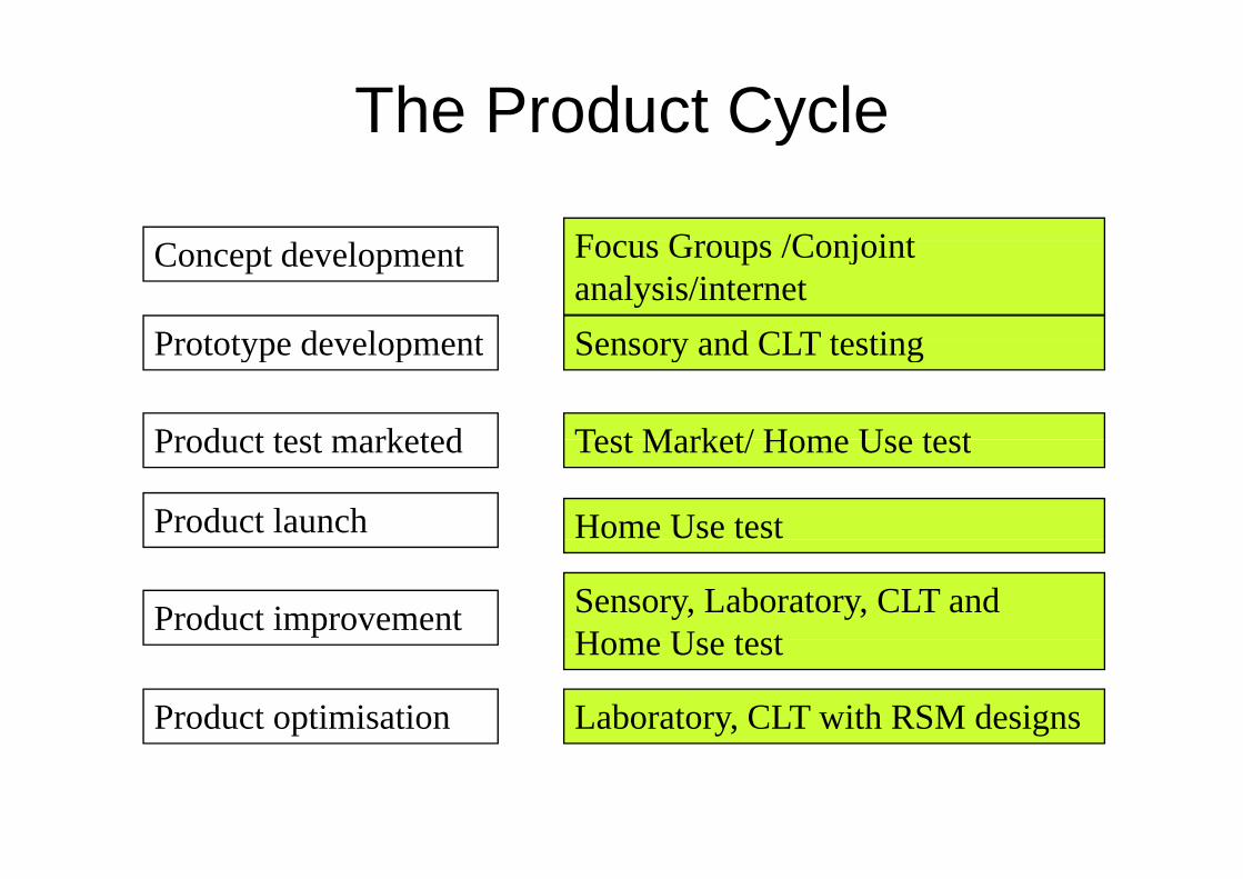
The Product Cycley
F G /C j i tConcept development
Prototype development
Focus Groups /Conjoint analysis/internetSensory and CLT testingPrototype development
Product test marketed
Sensory and CLT testing
Test Market/ Home Use testProduct test marketed
Product launch
Test Market/ Home Use test
Home Use test
Product improvement Sensory, Laboratory, CLT and Home Use test
Product optimisation
Home Use test
Laboratory, CLT with RSM designs

Hal MacFie TrainingHal MacFie Training
• Statistical Training for Sensory Professionals• Multivariate capabilityp y• Work inside Excel• Cheap enough to give license as part of course• Cheap enough to give license as part of course
feeCompatible with Office particularly PowerPoint• Compatible with Office, particularly PowerPoint
• Good Help• Tutorials

www halmacfie comwww.halmacfie.com
Anne Hasted

Specialised Computer TrainingSpecialised Computer Training Facilities
Cheaper than hotels
Easier to deal with easier to cancelEasier to deal with, easier to cancel

Location: MediaTek Training Facilities 90 Broad Street90 Broad Street
11th Floor New York, NY 10004
Entrance Training Room
E-mail area Break area

Hands on CoursesHands on Courses• Sensory statistics• Sensory statistics
– Anova, Non parametric, PCA, GPA cluster, Discriminant and Canonical Variates, PLS,
• Preference Mapping and Consumer Testing– Anova, PCA, Cluster, PCA, Internal Preference
M i E t l P f i PLSMapping, External Preference mapping, PLS• Since 2002, for each course
2 public offerings per year and approximately 3 in– 2 public offerings per year and approximately 3 in-house courses per year
• France, UK, Belgium, Ireland, Sweden, , , g , , ,Switzerland, USA, Israel, Mexico, Brazil, South Africa, China, Thailand, Australia

It is important to relax before you do a course in a new country!

Hands on FormulaHands on FormulaL t 45 i t 1 h• Lecture 45 mins to 1 hour
• Hands on exercising with fully worked solutions 30fully worked solutions 30 mins
• Attendees save their work on to a CD at the end of the course
• Should be able to redo• Should be able to redo exercises in 6 months to remind themselves of how to conduct and interpret the data

XLSTAT featuresXLSTAT features
• Sitting inside Excel means easy access
• Data input in many stats packages is complex
• Messages appear when you hover over

XLSTAT featuresXLSTAT features
• Multiple plotting is easy with labels

XLSTAT featuresXLSTAT features
60
• Coloring up the labels is easy
Royal Gala
40
50
gd
Braeburn
Top Red Pink Lady
Golden Delicious
Johnson's Red
20
30
E_Ye
llow
bac
kg
Sun Gold
Braeburn
Fuji
Granny Smith
Gibson's Green
0
10
0 10 20 30 40 50 60 70 800 10 20 30 40 50 60 70 80
E_Green backgd

XLSTAT featuresXLSTAT features• After a PCA shows three components large, it is
easy to do a quick 3d bubble plotScree plot
Factor scores:
Observation F1 F2 F3
8
10
12
14
16
enva
lue
60
80
100
e va
riabi
lity
(%)
Observation F1 F2 F3Gibson's Green 0.675 5.228 -0.905Johnson's Red 5.210 -1.449 -0.965Golden Delicious -0.854 2.352 -0.923Granny Smith -5.812 0.429 2.305Pink Lady -2.154 -3.632 -0.922
Gibson's Green
6
0
2
4
6
F1 F2 F3 F4 F5 F6 F7 F8 F9
axis
Eige
0
20
40
Cum
ulat
ive Fuji -0.807 1.414 -0.828
Top Red 2.902 0.450 4.990Braeburn -0.339 -0.278 -3.088Royal Gala 5.517 -1.942 0.154Sun Gold -4.338 -2.570 0.180
Golden Delicious
Gibson s Green
2
4
Braeburn
Fuji
Granny Smith Top Red0
2
-10 -5 0 5 10
F2
Johnson's Red
Pink Lady
Royal Gala
Sun Gold
-4
-2
F1
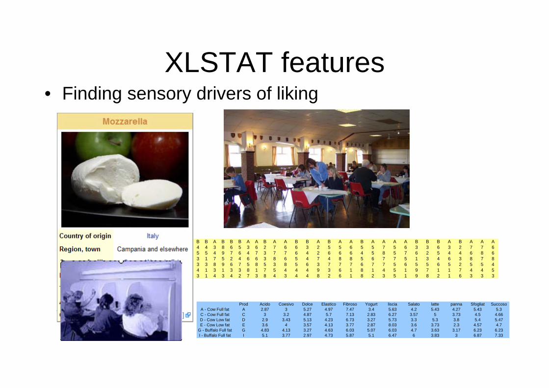
XLSTAT featuresXLSTAT features• Finding sensory drivers of liking
B B A B B B A A B A A B B A B A A B A A A A B B B A B A A A4 4 3 8 6 5 3 6 2 7 6 6 3 2 5 5 6 5 5 7 5 6 3 3 6 3 2 7 7 65 5 4 9 7 6 4 7 3 7 7 6 4 2 6 6 6 4 5 8 5 7 6 2 5 4 4 6 8 63 1 7 5 2 4 6 6 3 8 6 5 4 7 4 8 8 5 6 7 7 5 1 3 4 6 3 8 7 83 3 8 9 6 7 5 8 5 3 8 5 6 3 7 7 7 6 7 7 5 6 5 5 6 5 2 5 5 44 1 3 1 3 3 8 1 7 5 4 4 4 9 3 6 1 8 1 4 5 1 9 7 1 1 7 4 4 53 1 4 3 4 2 7 3 8 4 3 4 4 8 2 6 1 8 2 3 5 1 9 8 2 1 6 3 3 3
Prod Acido Coesivo Dolce Elastico Fibroso Yogurt liscia Salato latte panna Sfogliat SuccosoA - Cow Full fat A 2.87 3 5.27 4.97 7.47 3.4 5.63 4.2 5.43 4.27 5.43 5.3C - Cow Full fat C 3 3.2 4.87 5.7 7.13 2.83 6.27 3.57 5 3.73 4.5 4.66D - Cow Low fat D 2.9 3.43 5.13 4.23 6.73 3.27 5.73 3.3 5.3 3.8 5.4 5.47E - Cow Low fat E 3.6 4 3.57 4.13 3.77 2.87 8.03 3.6 3.73 2.3 4.57 4.7E Cow Low fat E 3.6 4 3.57 4.13 3.77 2.87 8.03 3.6 3.73 2.3 4.57 4.7
G - Buffalo Full fat G 4.83 4.13 3.27 4.63 6.03 5.07 6.03 4.7 3.63 3.17 6.23 6.23I - Buffalo Full fat I 5.1 3.77 2.97 4.73 5.87 5.1 6.47 6 3.83 3 6.87 7.33

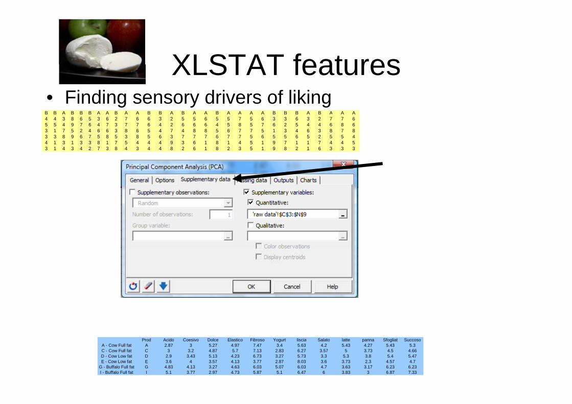
XLSTAT featuresXLSTAT features• Finding sensory drivers of liking
B B A B B B A A B A A B B A B A A B A A A A B B B A B A A A4 4 3 8 6 5 3 6 2 7 6 6 3 2 5 5 6 5 5 7 5 6 3 3 6 3 2 7 7 65 5 4 9 7 6 4 7 3 7 7 6 4 2 6 6 6 4 5 8 5 7 6 2 5 4 4 6 8 63 1 7 5 2 4 6 6 3 8 6 5 4 7 4 8 8 5 6 7 7 5 1 3 4 6 3 8 7 83 3 8 9 6 7 5 8 5 3 8 5 6 3 7 7 7 6 7 7 5 6 5 5 6 5 2 5 5 44 1 3 1 3 3 8 1 7 5 4 4 4 9 3 6 1 8 1 4 5 1 9 7 1 1 7 4 4 53 1 4 3 4 2 7 3 8 4 3 4 4 8 2 6 1 8 2 3 5 1 9 8 2 1 6 3 3 3
Prod Acido Coesivo Dolce Elastico Fibroso Yogurt liscia Salato latte panna Sfogliat SuccosoProd Acido Coesivo Dolce Elastico Fibroso Yogurt liscia Salato latte panna Sfogliat SuccosoA - Cow Full fat A 2.87 3 5.27 4.97 7.47 3.4 5.63 4.2 5.43 4.27 5.43 5.3C - Cow Full fat C 3 3.2 4.87 5.7 7.13 2.83 6.27 3.57 5 3.73 4.5 4.66D - Cow Low fat D 2.9 3.43 5.13 4.23 6.73 3.27 5.73 3.3 5.3 3.8 5.4 5.47E - Cow Low fat E 3.6 4 3.57 4.13 3.77 2.87 8.03 3.6 3.73 2.3 4.57 4.7
G - Buffalo Full fat G 4.83 4.13 3.27 4.63 6.03 5.07 6.03 4.7 3.63 3.17 6.23 6.23I - Buffalo Full fat I 5.1 3.77 2.97 4.73 5.87 5.1 6.47 6 3.83 3 6.87 7.33

XLSTAT featuresXLSTAT features• Finding sensory drivers of liking
Variables (axes F1 and F2: 74.77 %)
B BB
Fibroso1
Observations (axes F1 and F2: 74.77 %)
A
B
BB
B
B
BA
B
BA
A
B
B
A
A B
B
A
BB
A
A
B
B
A
AB
AB B
B
AB
A
AAA A
AB
B
A
B
B
Sfogliat
panna
latteElastico
Dolce
0.25
0.5
0.75
%)
G - Buffalo Full fat D - Cow Low fat
C - Cow Full fat
A - Cow Full fat
0
5
B
B
B
AA
B
B
A
BB
BBB
A
BB
AA
AA
A
B
AB
B
B AB
AB
B
A
AB
B
B
AA A
AB
A
AB
A
AB
AA
B
BB
Succoso
Sfogliat
SalatoYogurt
Acido
0 5
-0.25
0
0.25
F2 (2
0.31
%
I - Buffalo Full fat
-5
0F2
(20.
31 %
)
A
B
A ABB
B
B
B BB
BB A
B
Aliscia
Coesivo
-1
-0.75
-0.5
-1 -0.75 -0.5 -0.25 0 0.25 0.5 0.75 1E - Cow Low fat
-10
5
F1 (54.46 %)
Active variables Supplementary variables
-15 -10 -5 0 5 10
F1 (54.46 %)
Th d i f liki f B ff l d l lThe sensory drivers of liking for Buffalo and cow samples are clear

Xlstat MX Special Sensory ModuleXlstat MX– Special Sensory Module
• Generalised Procrustes Analysis GPA• Preference mapping (External)Preference mapping (External)• Penalty Analysis

Free Choice ProfilingFree Choice Profiling• Each assessor or respondents rates the products using
their own vocabulary• May be generated from lists or using triadic elicitation
(repertory grid )Triadic ElicitationTriadic Elicitation
Which pair of products in this triad are more similar to each other?other?
In what way are they more similar to each other than the third?

Generalized Procrustes AnalysisGeneralized Procrustes Analysis• In Greek mythology Procrustes (the stretcher) also known as Damastes• In Greek mythology, Procrustes (the stretcher), also known as Damastes
(subduer) and Polypemon (harming much), was a bandit from Attica. • iron bed into which he invited every passerby to lie down. • If the guest proved too tall, he would amputate the excess length; if theIf the guest proved too tall, he would amputate the excess length; if the
victim was found too short, he was then stretched out on the rack until he fit. Nobody would ever fit in the bed because it was secretly adjustable: Procrustes would stretch or shrink it upon sizing his victims from afar.
• Procrustes continued his reign of terror until he was captured by Theseus• Procrustes continued his reign of terror until he was captured by Theseus, who "fitted" Procrustes to his own bed and cut off his head and feet (since Theseus was a stout fellow, the bed had been set on the short position). Killing Procrustes was the last adventure of Theseus on his journey from Troezen to AthensTroezen to Athens.
• [edit] Derived meanings• A Procrustean bed is an arbitrary standard to which exact conformity is
forced. Sometimes the term is applied to the pan and scan process offorced. Sometimes the term is applied to the pan and scan process of cropping motion pictures for television and home video.

Generalized Procrustes AnalysisGeneralized Procrustes Analysis
Hotel
•Procrustes continued his reign of terror until he was captured by Theseus, who "fitted" P hi b d d ff hiProcrustes to his own bed and cut off his head and feet (since Theseus was a stout fellow, the bed had been set on the short position). Killing Procrustes was the last p ) gadventure of Theseus on his journey from Troezen to Athens.

GPA analysis averages matrices of different width
DescriptorsDescriptorsAssessor 1
A 2Assessor 2
Assessor 3m
ples
Sam

Application of GPA to the beer dataFRED JOHN KATE SUEoverall opinion overall opinion overall opinion overall opiniondark appearance light appearance dark appearance dark coloramount of head amount of color amount of head light colorlight appearance constant head thick head foamy appearancecarbonated appearance thin,watery head foamy headamount of color long lasting head light appearancelong lasting head frothy headhearty appearance golden colorfizzy appearancefizzy appearance
TOM JILL ANDY SIDoverall opinion overall opinion overall opinion thick appearancelight color pale appearance dark color coats glasscreamy head dark color appearance amount of head holds head for a long timeamount of head light appearance caramel color brown light colordark color carbonated appearance yellow color dark colorgolden color golden color appearance depth of shade amount of headduration of head amount of head overall opinion
fluffy appearancegolden brown appearancegolden-brown appearanceflat appearancebubbly appearance
• First point is that each person derived a different number of attributes• Applied GPA version that has recently become available in XLSTAT which
i ll fi ti t b th irequires all assessor configurations to be the same size

Application of GPA to the rep grid beer data
• There are 8 configurations one for each respondent• There are 8 configurations – one for each respondent• We want to do scaling, rotation and calculate a principal components
analysis on the consensus configuration.

Application of GPA to the rep grid beer data
Note I have only requested two dimensions here

Application of GPA to the beer data
Objects (axes F1 and F2: 76.75 %)
10
LLC
L
L
CB
A L
L
5FREDJOHNKATESUE
GFE
DC
B
A
L
KH
F
E D
C
BA
K
GF
ED
BA
L
K
H G
F
EC
BA
JH G
F
E
DC
BA
L
KH G
ED
CB
A
G
CB
H
FEDC
BA
KH GFED
CBA
0
TOMJILLANDYSIDConsensus
K
J
I
H
J
IGF
IH
J
I
DKJ
I
E
J I
FE KJIH F
ED
K
JI
GJ I
H Consensus
Th iti f h d t th d f
J
-5-5 0 5 10
-- axis F1 (56.61 %) -->
• The position of each product on the consensus and for each respondent is then plotted

Application of GPA to the beer dataVariables (axes F1 and F2: 76.75 %)
1
fred meanfred meanamount of headoverall opinion
overall opinion
kate meankate meankate meankate meankate mean
thick head
amount of headoverall opinion
overall opinion
ld b
overall opinion
sid meansid meansid meansid mean
amount of head
light color
holds head for a long time
0 5
1
fred meanfred mean
hearty appearance
long lasting head
amount of colorlight
dark appearance
j hj hj hfrothy headlong lasting
thin,watery head
light appearance
overall opinionlight
appearancefoamy head
dark appearance
sue meansue meansue meansue meansue meansue meansue meandark colortom meantom meantom meantom mean
duration of head
dark color
amount of headcreamy head
light color
overall opinionbubbly
golden-brown appearancefluffy
appearanceamount of head
carbonated appearance
light appearance
dark color appearance
pale appearance
overall opinion
andy meanandy meanandy meanandy meanandy mean
l l
amount of head
sid meansid meansid meansid meanlight color
coats glass
overall opinion
0
0.5
FREDJOHNKATESUE
fizzy appearancecarbonated appearance
gappearance john meanjohn meanjohn mean
long lasting headconstant head
amount of colorfoamy
appearancelight color
duration of headoverall opinionappearance
flat appearance
appearanceappearance appearancep
depth of shadeyellow color
caramel color brown
dark colordark color
coats glass
thick appearance
-0 5
0TOMJILLANDYSID
golden color
light colorgolden color
golden color appearance
-1
0.5
The position of each variable on the consensus and for each
1-1 -0.5 0 0.5 1
-- axis F1 (56.61 %) -->
• The position of each variable on the consensus and for each respondent is then plotted. This is the plot we use to determine which attributes are used consistently and go in the lexicon.
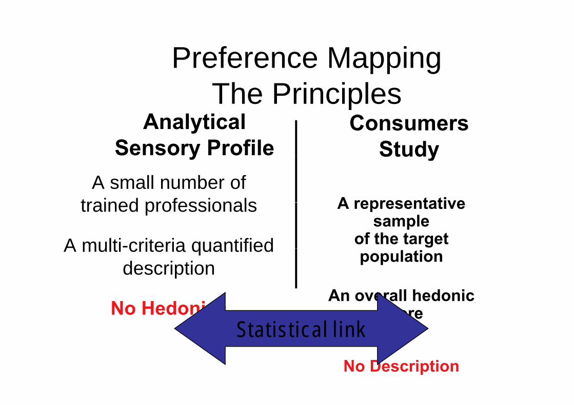
Preference MappingPreference MappingThe Principles
AnalyticalSensory Profile
ConsumersStudy
A small number of trained professionals A representative
y Study
trained professionals
A multi-criteria quantified
A representative sample
of the target A multi criteria quantified description
population
An overall hedonicNo Hedonics
An overall hedonic score
Statistical link
No Description

Preference Mapping
Sensory attributes
AnalyticalSensory Profile
ConsumersStudyThe Application
Hedonic Scores
Expertucts
Sensory attributes Hedonic Scores
ucts p1
0 10
√√ 3
8p
data
Prod
u
Prod
p8
p4√
√8
2
Dataanalysis
scores givenby 1 consumer
p1p3 p c sc
ore
5
10
p4
p3
p2
p5
p6
p7
p8
Hed
onic
0
5
2 0 202
p2
Products' expert mapAxis 2 Axis 1
-2 0-2
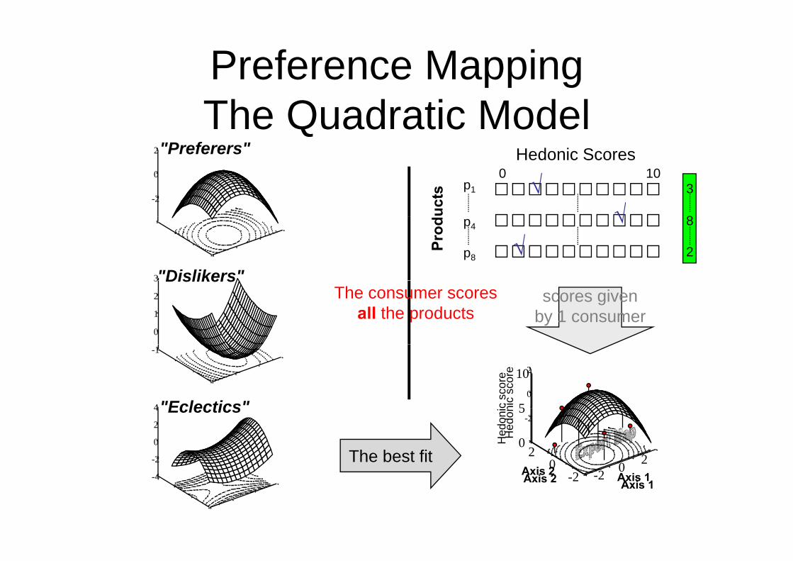
Preference Mapping
2"Preferers"The Quadratic Model
Hedonic Scores
-2
0
2 Preferers Hedonic Scores
ucts p1
0 10
√√ 3
8
3"Dislikers"
Prod
p8
p4√
√8
2
scores givenby 1 consumer
0
1
2
3 DislikersThe consumer scores
all the products
c sc
ore
5
10
4"Eclectics"
-1
0
2
nic
scor
eH
edon
ic
0
5
2 0 202The best fit -2
0
2
4 Eclectics-2
Axis 2
Hed
on
Axis 2 Axis 1-2 0
-2-4 Axis 2 Axis 1

Preference Mapping
Sensory attributes
pp gModelising all the consumers
Consumers
Expertucts
Sensory attributes
Hedonic scores
Consumers
ucts
pdata
Prod
u Hedonic scores
Prod
Dataanalysis
scores givenby 1 consumer
3
43
24
P3 P17p1p3 p c sc
ore
5
10
45678
1
2
3
4
P3 P1
P6
6
0
1
2
3
6
66
7
P8
P4
P1
P67p4
p3
p2
p5
p6
p7
p8
Hed
onic
0
5
2 0 202
6 80123451234
-2
-1
0
1 P8
P4
P7P5
P6
-6 -4 -2 0 2 4 6
-3
-2
-1 56
3
5
6P2
P7P5
5
4
p2
Products' expert mapAxis 2 Axis 1
-2 0-2
-8 -6 -4 -2 0 2 4 6 8
-4-3-2-10
-6 -4 -2 0 2 4 6
-3 P2

Preference Mapping
Sensory attributes
The Quadratic ResultConsumers
Expertucts
Sensory attributes
Hedonic scores
Consumers
ucts
pdata
Prod
u Hedonic scores
Prod
Dataanalysis
p1p3 p
p4
p3
p2
p5
p6
p7
p8
p2
Products' expert map

Consumer preferences andanalytical sensory description
A i 2Axis 1
(34.31 %)
Axis 2(30.36 %)

Consumer preferences andanalytical sensory description
3
4
POAFPLPF
50%
50%
60%
GreasyGreasyShinyShiny
1
2
PANC PFCF20% 30% 60%
H tH t
OdorousOdorous
0
PCRC
PPCF PCOF40%
70%
Axi
s 2
(30.
56 %
)
ColorColor
HeterogeneousHeterogeneous
-2
-1PCRC
PFDFPANF
PKSF
80%
RtdPORtdPOMatMat
GrainyGrainy
FirmFirmCompactCompact
StickySticky
-3
PPDC
PKSF
SmoothSmooth
FirmFirmClearClear
-5 -4 -3 -2 -1 0 1 2 3 4 5-4
Axis 1(32.91 %)

size 359 242 605Class cluster 1 clister 2 overallGibson's Green 5.059 4.304 4.760J h ' R d 4 608 8 232 6 064
We transpose and collect the ll i t Johnson's Red 4.608 8.232 6.064
Golden Delicious 6.876 7.125 6.958Granny Smith 6.263 3.756 5.260Pink Lady 6.046 4.860 5.573Fuji 4.469 6.712 5.378Top Red 2.889 6.662 4.421
overall means into anew table
Top Red 2.889 6.662 4.421Braeburn 5.893 4.704 5.420Royal Gala 3.892 6.683 5.028Sun Gold 7.071 4.493 6.043
Select cluster meansSelect cluster means as pref data
Regress on the first 2
PC’s.
No need for preliminary transformation as wetransformation as we have already done it.
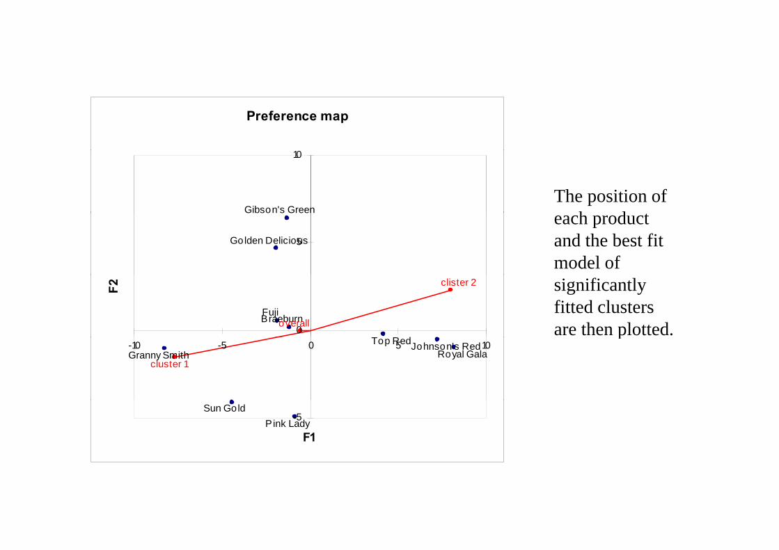
Preference map
The position of h dGibson's Green
10
each product and the best fit model of
Golden Delicious
Gibson s Green
5
significantly fitted clusters are then plotted.
Braeburn
T R d
Fujioverall
clister 2
0
F2
pRoyal Gala
Top RedGranny Smith
Johnson's Red
cluster 1
-10 -5 0 5 10
Sun GoldPink Lady-5
F1

S51
Contour plot
S31
S36
S41
S46
80%-100%
S11
S16
S21
S26F2 60%-80%
40%-60%
20%-40%
0%-20%
S1
S6
F1
The need for two products is clear in the contour plot

Mean Drop/Penalty AnalysisMean Drop/Penalty Analysis• Consumers make simple rating of product attributes p g p
using diagnostic scales
Di ti “J t b t Ri ht” JAR lDiagnostic “Just about Right” JAR scales
1 Much too Weak
2 Too Weak
3 OK Just about Right3 OK Just about Right
4 Too Strong
5 Much too Strong•If an attribute is not at its optimum level does it have anIf an attribute is not at its optimum level does it have an impact on product liking?

Mean Drop/Penalty AnalysisMean Drop/Penalty Analysis
1
Percentages for the JAR levels
1
Percentages for the JAR levels (collapsed)
0 5
0.6
0.7
0.8
0.9
% 0 5
0.6
0.7
0.8
0.9
%
0.1
0.2
0.3
0.4
0.5%
0.1
0.2
0.3
0.4
0.5%
0Flavour JAR Garlic JAR Sweetness JAR Saltiness JAR
1 2 3 4 5
0Flavour JAR Garlic JAR Sweetness JAR Saltiness JAR
Too little JAR Too much

Mean Drop for Flavour on AMean Drop for Flavour on AMean Drop
Mean(Liking)
Mean Drop
7.0008.0009.000
3 0004.0005.0006.000
15% 35% 50%
0.0001.0002.0003.000 15% 35% 50%
Too little JAR Too much
Th i th t th i t h flThe consensus is that there is too much flavour

Mean Drop for Flavour on AMean Drop for Flavour on AMean drops vs %p
Flavour JAR
2.5
3
Garlic JAR
Flavour JAR
1.5
2ro
ps
Saltiness JAR
Sweetness JAR
Sweetness JAR
Garlic JAR
0
0.5
1
Mea
n d
Saltiness JAR
-1
-0.50 10 20 30 40 50 60 70
%
Th i th t th i t h fl d t littl G li
%
Too little Too much
The consensus is that there is too much flavour and too little Garlic

Multiple Factor Analysis (MFA)Multiple Factor Analysis (MFA)
• A new method to provide a map of several tables of data on the same samples from pdifferent sources and with different numbers of variablesnumbers of variables
• The weighting of the tables makes it possible to ensure the tables with more variables do not weight too heavily in the g yanalysis.

MFA Graphicp
Table 1 Table 2 Table 3Table 1
PCA MCA PCA or MCAPCA or MCA PCA or MCA
E1 E2 E3E1 E2 E3
/E2/E1 /E2/E1/E3
APCA
A B
C D

Loire Wine dataLoire Wine dataPE
LATI
IL ST1
ST2
ST3
ST4
ST5
ION
1
ION
2
ION
3
AK
E1
AK
E2
AK
E3
AK
E4
AK
E5
AK
E6
AK
E7
AK
E8
AK
E9
AK
E10
STE1
STE2
STE3
STE4
ID AP P
SOI
RES
RES
RES
RES
RES
VIS
VIS
VIS
SHA
SHA
SHA
SHA
SHA
SHA
SHA
SHA
SHA
SHA
TAS
TAS
TAS
TAS
2EL Saumur Mil1 3.074 3 2.714 2.28 1.96 4.321 4 3.269 3.407 3.308 2.885 2.32 1.84 2 1.65 3.259 2.963 3.2 2.963 2.107 2.429 2.51CHA Saumur Mil1 2.964 2.821 2.375 2.28 1.68 3.222 3 2.808 3.37 3 2.56 2.44 1.739 2 1.381 2.962 2.808 2.926 3.036 2.107 2.179 2.6541FON Bourgueuil Mil1 2.857 2.929 2.56 1.96 2.077 3.536 3.393 3 3.25 2.929 2.769 2.192 2.25 1.75 1.25 3.077 2.8 3.077 3.222 2.179 2.25 2.6431VAU Chinon Mil2 2.808 2.593 2.417 1.913 2.16 2.893 2.786 2.538 3.16 2.88 2.391 2.083 2.167 2.304 1.476 2.542 2.583 2.478 2.704 3.179 2.185 2.51DAM Saumur Ref 3.607 3.429 3.154 2.154 2.04 4.393 4.036 3.385 3.536 3.36 3.16 2.231 2.148 1.762 1.6 3.615 3.296 3.462 3.464 2.571 2.536 2.7862BOU B il R f 2 857 3 111 2 577 2 04 2 077 4 464 4 259 3 407 3 179 3 385 2 8 2 24 2 148 1 75 1 476 3 214 3 148 3 321 3 286 2 393 2 643 2 8572BOU Bourgueuil Ref 2.857 3.111 2.577 2.04 2.077 4.464 4.259 3.407 3.179 3.385 2.8 2.24 2.148 1.75 1.476 3.214 3.148 3.321 3.286 2.393 2.643 2.8571BOI Bourgueuil Ref 3.214 3.222 2.962 2.115 2.04 4.143 3.929 3.25 3.429 3.5 3.038 2.2 2.385 1.826 1.476 3.25 3.222 3.385 3.393 2.607 2.607 2.7783EL Saumur Mil1 3.12 2.852 2.5 2.2 2.185 4.214 3.857 3.077 3.654 3.077 2.52 2.32 2.444 2.08 1.905 3.28 3.16 2.962 3.25 2.179 2.63 2.778DOM1 Chinon Mil1 2.857 2.815 2.808 1.923 2.074 4.037 3.893 3.28 3.357 3.346 3 2.04 2.125 1.875 1.524 3.148 2.893 3.308 3.286 2.286 2.407 2.7411TUR Saumur Mil2 2.893 3 2.571 1.846 1.68 3.704 3.407 3.111 3.222 3.259 2.926 2.04 2.042 2 1.773 3.077 2.704 2.778 2.893 2.357 2.25 2.7044EL Saumur Mil2 3.25 3.286 2.714 1.926 1.962 3.857 3.643 3.259 3.607 3.385 2.889 2.115 2.16 1.955 1.571 3.286 3.036 3.222 3.321 2.429 2.571 2.893PER1 Saumur Mil2 3.393 3.179 2.769 2.038 1.92 4.714 4.5 3.321 3.481 3.385 2.962 2 2.2 2.042 1.545 3.321 3.071 3.143 3.357 2.429 2.607 2.821
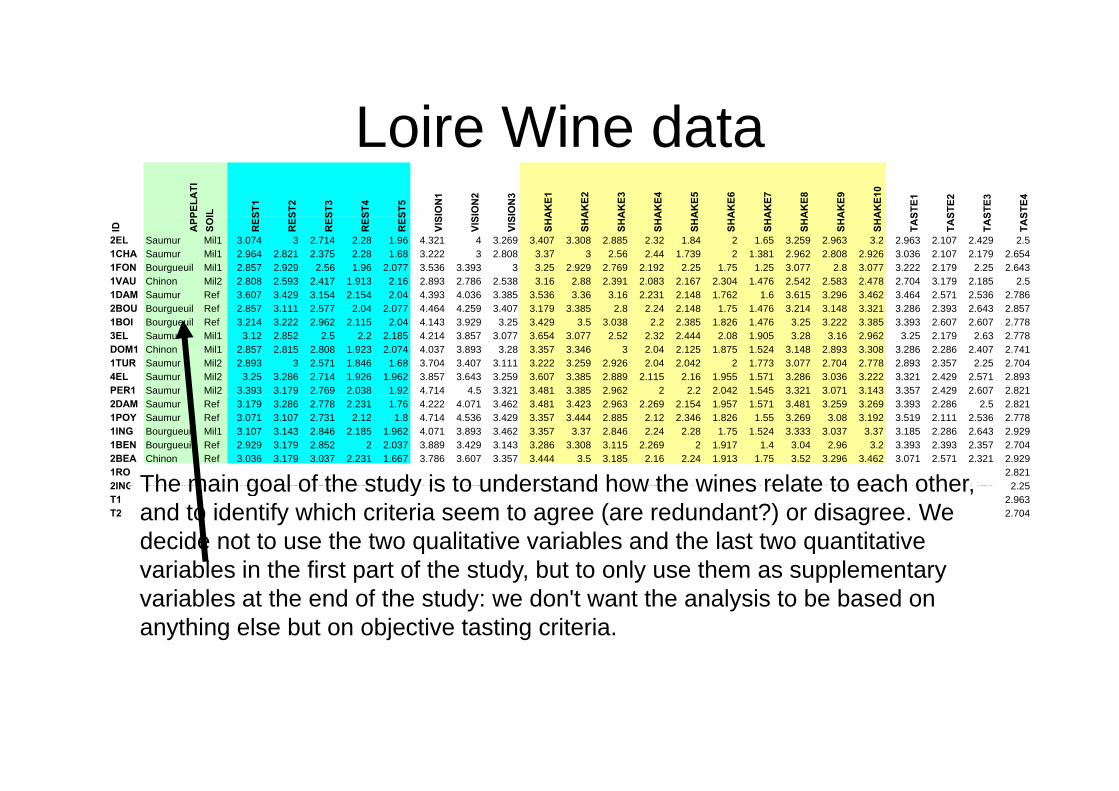
The data correspond to the tasting of 21 wines from the Loire region in France by 36 experts. The data set comprises 21 observations
2DAM Saumur Ref 3.179 3.286 2.778 2.231 1.76 4.222 4.071 3.462 3.481 3.423 2.963 2.269 2.154 1.957 1.571 3.481 3.259 3.269 3.393 2.286 2.5 2.8211POY Saumur Ref 3.071 3.107 2.731 2.12 1.8 4.714 4.536 3.429 3.357 3.444 2.885 2.12 2.346 1.826 1.55 3.269 3.08 3.192 3.519 2.111 2.536 2.7781ING Bourgueuil Mil1 3.107 3.143 2.846 2.185 1.962 4.071 3.893 3.462 3.357 3.37 2.846 2.24 2.28 1.75 1.524 3.333 3.037 3.37 3.185 2.286 2.643 2.9291BEN Bourgueuil Ref 2.929 3.179 2.852 2 2.037 3.889 3.429 3.143 3.286 3.308 3.115 2.269 2 1.917 1.4 3.04 2.96 3.2 3.393 2.393 2.357 2.7042BEA Chinon Ref 3.036 3.179 3.037 2.231 1.667 3.786 3.607 3.357 3.444 3.5 3.185 2.16 2.24 1.913 1.75 3.52 3.296 3.462 3.071 2.571 2.321 2.9291ROC Chinon Mil2 3.071 2.926 2.741 2 1.88 3.679 3.393 3.192 3.37 3.36 2.963 2.308 1.917 2 1.429 3.25 2.92 2.88 3.071 2.393 2.321 2.8212ING Bourgueuil Mil1 2 643 2 786 2 536 1 889 1 808 2 607 2 536 2 444 2 889 2 8 2 5 1 962 2 111 2 08 1 318 2 68 2 308 2 556 2 179 2 25 1 964 2 25
y p pand 31 dimensions. The 31 dimensions can grouped into 6 categories:- the first 2 qualitative variables are related to the geography
2ING Bourgueuil Mil1 2.643 2.786 2.536 1.889 1.808 2.607 2.536 2.444 2.889 2.8 2.5 1.962 2.111 2.08 1.318 2.68 2.308 2.556 2.179 2.25 1.964 2.25T1 Saumur Mil4 3.696 3.192 2.833 1.826 2.385 4.321 4 3.333 3.737 3.08 2.833 1.773 2.44 2.292 1.571 3.437 2.958 2.6 2.963 2.407 2.643 2.963T2 Saumur Mil4 3.708 2.926 2.52 2.04 2.667 4.321 4.107 3.259 3.727 2.885 2.6 2.083 2.609 2.174 1.65 3.095 3.136 2.545 3.333 2.571 2.667 2.704
(appellation and soil);- the next 5 quantitative variables correspond to the olfaction after rest;- the next 3 quantitative variables correspond to visual criteria;- the next 10 quantitative variables correspond to the olfaction after shaking;
th t 9 tit ti i bl d t th t t- the next 9 quantitative variables correspond to the taste;- the last 2 quantitative variables correspond to global ratings.
Loire Wine dataLoire Wine dataPE
LATI
IL ST1
ST2
ST3
ST4
ST5
ION
1
ION
2
ION
3
AK
E1
AK
E2
AK
E3
AK
E4
AK
E5
AK
E6
AK
E7
AK
E8
AK
E9
AK
E10
STE1
STE2
STE3
STE4
ID AP P
SOI
RES
RES
RES
RES
RES
VIS
VIS
VIS
SHA
SHA
SHA
SHA
SHA
SHA
SHA
SHA
SHA
SHA
TAS
TAS
TAS
TAS
2EL Saumur Mil1 3.074 3 2.714 2.28 1.96 4.321 4 3.269 3.407 3.308 2.885 2.32 1.84 2 1.65 3.259 2.963 3.2 2.963 2.107 2.429 2.51CHA Saumur Mil1 2.964 2.821 2.375 2.28 1.68 3.222 3 2.808 3.37 3 2.56 2.44 1.739 2 1.381 2.962 2.808 2.926 3.036 2.107 2.179 2.6541FON Bourgueuil Mil1 2.857 2.929 2.56 1.96 2.077 3.536 3.393 3 3.25 2.929 2.769 2.192 2.25 1.75 1.25 3.077 2.8 3.077 3.222 2.179 2.25 2.6431VAU Chinon Mil2 2.808 2.593 2.417 1.913 2.16 2.893 2.786 2.538 3.16 2.88 2.391 2.083 2.167 2.304 1.476 2.542 2.583 2.478 2.704 3.179 2.185 2.51DAM Saumur Ref 3.607 3.429 3.154 2.154 2.04 4.393 4.036 3.385 3.536 3.36 3.16 2.231 2.148 1.762 1.6 3.615 3.296 3.462 3.464 2.571 2.536 2.7862BOU B il R f 2 857 3 111 2 577 2 04 2 077 4 464 4 259 3 407 3 179 3 385 2 8 2 24 2 148 1 75 1 476 3 214 3 148 3 321 3 286 2 393 2 643 2 8572BOU Bourgueuil Ref 2.857 3.111 2.577 2.04 2.077 4.464 4.259 3.407 3.179 3.385 2.8 2.24 2.148 1.75 1.476 3.214 3.148 3.321 3.286 2.393 2.643 2.8571BOI Bourgueuil Ref 3.214 3.222 2.962 2.115 2.04 4.143 3.929 3.25 3.429 3.5 3.038 2.2 2.385 1.826 1.476 3.25 3.222 3.385 3.393 2.607 2.607 2.7783EL Saumur Mil1 3.12 2.852 2.5 2.2 2.185 4.214 3.857 3.077 3.654 3.077 2.52 2.32 2.444 2.08 1.905 3.28 3.16 2.962 3.25 2.179 2.63 2.778DOM1 Chinon Mil1 2.857 2.815 2.808 1.923 2.074 4.037 3.893 3.28 3.357 3.346 3 2.04 2.125 1.875 1.524 3.148 2.893 3.308 3.286 2.286 2.407 2.7411TUR Saumur Mil2 2.893 3 2.571 1.846 1.68 3.704 3.407 3.111 3.222 3.259 2.926 2.04 2.042 2 1.773 3.077 2.704 2.778 2.893 2.357 2.25 2.7044EL Saumur Mil2 3.25 3.286 2.714 1.926 1.962 3.857 3.643 3.259 3.607 3.385 2.889 2.115 2.16 1.955 1.571 3.286 3.036 3.222 3.321 2.429 2.571 2.893PER1 Saumur Mil2 3.393 3.179 2.769 2.038 1.92 4.714 4.5 3.321 3.481 3.385 2.962 2 2.2 2.042 1.545 3.321 3.071 3.143 3.357 2.429 2.607 2.8212DAM Saumur Ref 3.179 3.286 2.778 2.231 1.76 4.222 4.071 3.462 3.481 3.423 2.963 2.269 2.154 1.957 1.571 3.481 3.259 3.269 3.393 2.286 2.5 2.8211POY Saumur Ref 3.071 3.107 2.731 2.12 1.8 4.714 4.536 3.429 3.357 3.444 2.885 2.12 2.346 1.826 1.55 3.269 3.08 3.192 3.519 2.111 2.536 2.7781ING Bourgueuil Mil1 3.107 3.143 2.846 2.185 1.962 4.071 3.893 3.462 3.357 3.37 2.846 2.24 2.28 1.75 1.524 3.333 3.037 3.37 3.185 2.286 2.643 2.9291BEN Bourgueuil Ref 2.929 3.179 2.852 2 2.037 3.889 3.429 3.143 3.286 3.308 3.115 2.269 2 1.917 1.4 3.04 2.96 3.2 3.393 2.393 2.357 2.7042BEA Chinon Ref 3.036 3.179 3.037 2.231 1.667 3.786 3.607 3.357 3.444 3.5 3.185 2.16 2.24 1.913 1.75 3.52 3.296 3.462 3.071 2.571 2.321 2.9291ROC Chinon Mil2 3.071 2.926 2.741 2 1.88 3.679 3.393 3.192 3.37 3.36 2.963 2.308 1.917 2 1.429 3.25 2.92 2.88 3.071 2.393 2.321 2.8212ING Bourgueuil Mil1 2 643 2 786 2 536 1 889 1 808 2 607 2 536 2 444 2 889 2 8 2 5 1 962 2 111 2 08 1 318 2 68 2 308 2 556 2 179 2 25 1 964 2 25The main goal of the study is to understand how the wines relate to each other2ING Bourgueuil Mil1 2.643 2.786 2.536 1.889 1.808 2.607 2.536 2.444 2.889 2.8 2.5 1.962 2.111 2.08 1.318 2.68 2.308 2.556 2.179 2.25 1.964 2.25T1 Saumur Mil4 3.696 3.192 2.833 1.826 2.385 4.321 4 3.333 3.737 3.08 2.833 1.773 2.44 2.292 1.571 3.437 2.958 2.6 2.963 2.407 2.643 2.963T2 Saumur Mil4 3.708 2.926 2.52 2.04 2.667 4.321 4.107 3.259 3.727 2.885 2.6 2.083 2.609 2.174 1.65 3.095 3.136 2.545 3.333 2.571 2.667 2.704
The main goal of the study is to understand how the wines relate to each other, and to identify which criteria seem to agree (are redundant?) or disagree. We decide not to use the two qualitative variables and the last two quantitative variables in the first part of the study but to only use them as supplementaryvariables in the first part of the study, but to only use them as supplementary variables at the end of the study: we don't want the analysis to be based on anything else but on objective tasting criteria.
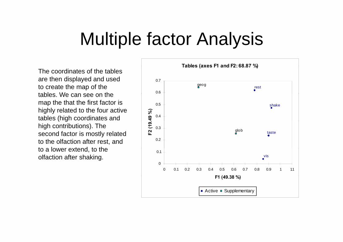
Multiple factor AnalysisMultiple factor AnalysisTables (axes F1 and F2: 68 87 %)Tables (axes F1 and F2: 68.87 %)
restgeog
0.6
0.7
The coordinates of the tables are then displayed and used to create the map of the tables We can see on the
shake
0.4
0.5
.49
%)
tables. We can see on the map the that the first factor is highly related to the four active tables (high coordinates and
tasteglob
0.2
0.3
F2 (1
9.
( ghigh contributions). The second factor is mostly related to the olfaction after rest, and to a lower extend to the
vis
0
0.1
0 0.1 0.2 0.3 0.4 0.5 0.6 0.7 0.8 0.9 1 1.1
F1 (49 38 %)
to a lower extend, to the olfaction after shaking.
F1 (49.38 %)
Active Supplementary

Multiple factor Analysisp yThe next chart shows the observations with the centroids of the two
Observations (axes F1 and F2: 68.87 %)centroids of the two qualitative variables. We can see that the T1 and T2 wines are very close, and isolated from the other
T2
T1
4
isolated from the other wines. They are highly related to the second factor, which, as we saw earlier, is highly related to Rest5 The
T1
2
3
%)
highly related to Rest5. The 1DAM wine has the highest coordinate on the first axis.
PER14EL
3EL1VAU
0
1F2
(19.
49 %
2ING1ROC
2BEA1BEN
1ING 1POY2DAM
1TUR DOM11BOI2BOU 1DAM
1FON
2EL-1
0
1CHA
-2-5 -4 -3 -2 -1 0 1 2 3 4
F1 (49.38 %)F1 (49.38 %)

The Future Path PLSThe Future – Path PLS
• PATH PLS is now released• Enab;es complex pathways for relationsEnab;es complex pathways for relations
between sensory categories and emotional and brand image attributes toemotional and brand image attributes to be built and the goodness of fit tested.

Possible Path model for Pref mappingPossible Path model for Pref mapping
D hiT t Cl t
Appearance
sensory DemographicsTaste Clusters
Appearance
Flavour/aroma
S
Flavour/aroma
ConsumerSensory Consumer Hedonics
Texture

SummarySummary
• Easy to use and input data• Inside Excel writes results to ExcelInside Excel, writes results to Excel• Useful Plotting• Excellent Multivariate suite• MX provides a uniquely useful resource to• MX provides a uniquely useful resource to
sensory and consumer scientists• On-going innovation (Path-PLS) keeps
momentum
![GTHandbook-final-edits-newThe thermodynamic path over which the gas turbine engine operates is the Brayton Cycle (Figure 1). The compressor [C] ingests and compresses ambient air to](https://static.fdocuments.net/doc/165x107/5e6a89ab41d8f5438502f590/gthandbook-final-edits-new-the-thermodynamic-path-over-which-the-gas-turbine-engine.jpg)


