THE USE OF RECURRENT NEURAL NETWORKS IN CONTINUOUS …

3

1

2

3

1

2

Mike Hochberg is now at Nuance Communications, 333 Ravenswood Avenue, Building110, Menlo Park, CA 94025, USA.

Steve Renals is now at the Department of Computer Science, University of She�eld,She�eld S1 4DP, UK.

This chapter was written in 1994. Further advances have been made such as: context-dependent phone modelling; forward-backward training and adaptation using linear inputtransformations.

This chapter describes a use of recurrent neural networks (i.e., feedback is incorpo-rated in the computation) as an acoustic model for continuous speech recognition.The form of the recurrent neural network is described along with an appropriate pa-rameter estimation procedure. For each frame of acoustic data, the recurrent networkgenerates an estimate of the posterior probability of of the possible phones given theobserved acoustic signal. The posteriors are then converted into scaled likelihoodsand used as the observation probabilities within a conventional decoding paradigm(e.g., Viterbi decoding). The advantages of using recurrent networks are that theyrequire a small number of parameters and provide a fast decoding capability (relativeto conventional, large-vocabulary, HMM systems) .

Most { if not all { automatic speech recognition systems explicitly or implicitlycompute a (equivalently, etc.) indicating how well aninput acoustic signal matches a speech model of the hypothesised utterance. Afundamental problem in speech recognition is how this score may be computed,

159

Cambridge University Engineering Department,

Trumpington Street, Cambridge, CB2 1PZ, U.K.

score distance, probability,

Tony Robinson, Mike Hochberg

and Steve Renals

ABSTRACT

1 INTRODUCTION

THE USE OF RECURRENT

NEURAL NETWORKS IN

CONTINUOUS SPEECH

RECOGNITION

7

4

4

1 2 T

�

W W

�

Throughout this chapter, the terms Pr and indicate the probability mass and theprobability density function, respectively.

p

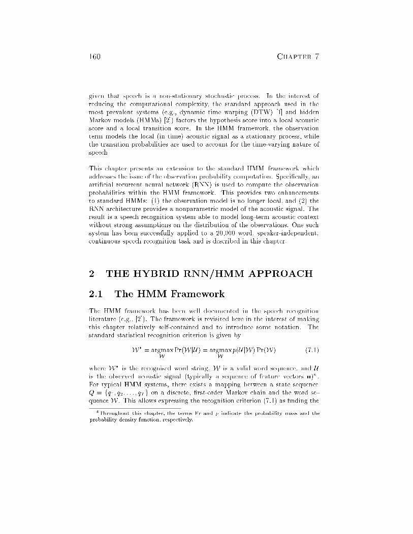
given that speech is a non-stationary stochastic process. In the interest ofreducing the computational complexity, the standard approach used in themost prevalent systems (e.g., dynamic time warping (DTW) [1] and hiddenMarkov models (HMMs) [2]) factors the hypothesis score into a local acousticscore and a local transition score. In the HMM framework, the observationterm models the local (in time) acoustic signal as a stationary process, whilethe transition probabilities are used to account for the time-varying nature ofspeech.

This chapter presents an extension to the standard HMM framework whichaddresses the issue of the observation probability computation. Speci�cally, anarti�cial recurrent neural network (RNN) is used to compute the observationprobabilities within the HMM framework. This provides two enhancementsto standard HMMs: (1) the observation model is no longer local, and (2) theRNN architecture provides a nonparametric model of the acoustic signal. Theresult is a speech recognition system able to model long-term acoustic contextwithout strong assumptions on the distribution of the observations. One suchsystem has been successfully applied to a 20,000 word, speaker-independent,continuous speech recognition task and is described in this chapter.

The HMM framework has been well documented in the speech recognitionliterature (e.g., [2]). The framework is revisited here in the interest of makingthis chapter relatively self-contained and to introduce some notation. Thestandard statistical recognition criterion is given by

= argmaxPr( ) = argmax ( ) Pr( ) (7.1)

where is the recognised word string, is a valid word sequence, andis the observed acoustic signal (typically a sequence of feature vectors ) .For typical HMM systems, there exists a mapping between a state sequence

= on a discrete, �rst-order Markov chain and the word se-quence . This allows expressing the recognition criterion (7.1) as �nding the

p

Q q ; q ; : : :; q

W WjU UjW W

W W U

f gW

u

160

2 THE HYBRID RNN/HMM APPROACH

2.1 The HMM Framework

Chapter 7

=1

1

1

Q

T

t

t t t t

t t

t t

m

qm qm qm

��

�

maximum a posteriori (MAP) state sequence of length , i.e.,

= argmax Pr( ) ( ) (7.2)

Note that the HMM framework has reduced the primary modelling requirementto stationary, local (in time) components; namely the observation terms ( )and transition terms Pr( ). There are a number of well known methodsfor modelling the observation terms. Continuous density HMMs typically useGaussian mixture distributions of the form

( ) = ( ; � ) (7.3)

Recently, there has been work in the area of hybrid connectionist/HMM sys-tems. In this approach, nonparametric distributions represented with neuralnetworks have been used as models for the observation terms [3, 4].

Context is very important in speech recognition at multiple levels. On a shorttime scale such as the average length of a phone, limitations on the rate ofchange of the vocal tract cause a blurring of acoustic features which is knownas co-articulation. Achieving the highest possible levels of speech recognitionperformance means making e�cient use of all the contextual information.

Current HMM technology primarily approaches the problem from a top-downperspective by modelling phonetic context. The short-term contextual in uenceof co-articulation is handled by creating a model for all su�ciently distinctphonetic contexts. This entails a trade o� between creating enough modelsfor adequate coverage and maintaining enough training examples per contextso that the parameters for each model may be well estimated. Clustering andsmoothing techniques can enable a reasonable compromise to be made at theexpense of model accuracy and storage requirements (e.g., [5, 6]).

Acoustic context in HMMs is typically handled by increasing the dimensionalityof the observation vector to include some parameterisation of the neighbour-ing acoustic vectors. The simplest way to accomplish this is to replace thesingle frame of parameterised speech by a vector containing several adjacentframes along with the original central frame. Alternatively, each frame can beaugmented with estimates of the temporal derivatives of the parameters [7].

T

Q q q p q :

p qq q

p q c u � ; :

j j

jj

j N

u

u

u

161Recurrent Networks

2.2 Context Modelling

Y

X

However, this dimensionality expansion quickly results in di�culty in obtain-ing good models of the data. Multi-layer perceptrons (MLPs) have been sug-gested as an approach to model high-order correlations of such high-dimensionalacoustic vectors. When trained as classi�ers, MLPs approximate the posteriorprobability of class occupancy [8, 9, 10, 11, 12]. For a full discussion of thisresult to speech recognition, see [13, 4].

Including feedback into the MLP structure gives a method of e�ciently incor-porating context in much the same way as an in�nite impulse response �lter canbe more e�cient than a �nite impulse response �lter in terms of storage andcomputational requirements. Duplication of resources is avoided by processingone frame of speech at a time in the context of an internal state as opposed toapplying nearly the same operation to each frame in a larger window. Feed-back also gives a longer context window, so it is possible that uncertain evidencecan be accumulated over many time frames in order to build up an accuraterepresentation of the long term contextual variables.

There are a number of possible methods for incorporating feedback into a speechrecognition system. One approach is to consider the forward equations of astandard HMM as recurrent network-like computation. The HMM can thenbe trained using the maximum likelihood criterion [14] or other discriminativetraining criteria [15, 16, 17]. Another approach is to use a recurrent networkonly for estimation of the emission probabilities in an HMM framework. Thisis similar to the hybrid connectionist-HMM approach described in [3] and isthe approach used in the system described in this chapter.

The form of the recurrent network used here was �rst described in [18]. Thepaper took the basic equations for a linear dynamical system and replaced thelinear matrix operators with non-linear feedforward networks. After mergingcomputations, the resulting structure is illustrated in �gure 1. The currentinput, ( ), is presented to the network along with the current state, ( ). Thesetwo vectors are passed through a standard feed-forward network to give theoutput vector, ( ) and the next state vector, ( + 1). De�ning the combinedinput vector as ( ) and the weight matrices to the outputs and the next state

t t

t tt

u x

y x

z

162

2.3 Recurrent Networks for PhoneProbability Estimation

Chapter 7

u(t)

x(t+1)x(t)

Timedelay

y(t)

1

ii

j j

ii

i

i t t

i

The recurrent network used for phone probability estimation.

as and , respectively:

( ) =1( )( )

(7.4)

( ) =exp( ( ))

exp( ( ))(7.5)

( + 1) =1

1 + exp( ( ))(7.6)

The inclusion of \1" in ( ) provides the mechanism to apply a bias to thenon-linearities. As is easily seen in (7.4){(7.6), the complete system is no morethan a large matrix multiplication followed by a non-linear function.

A very important point to note about this structure is that if the parameters areestimated using certain training criteria (see section 4), the network outputs areconsistent estimators of class posterior probabilities. Speci�cally, the outputs( ) are interpreted as

( ) = Pr( = (0)) (7.7)

The softmax non-linear function of (7.5) is an appropriate non-linearity for es-timating posterior probabilities as it ensures that the values are non-negativeand sum to one. Work on generalised linear models [19] also provides theoret-ical justi�cation for interpreting ( ) as probabilities. Similarly, the sigmoidalnon-linearity of (7.6) is the softmax non-linearity for the two class case and

t tt

y tt

t

x tt

t

y t

y t q i u ; : : : ; u ; :

y t

�

j

W V

z u

x

W z

W z

V z

z

x


24

35

P

Figure 1

0 0.2 0.4 0.6 0.8 10.5

0.55

0.6

0.65

0.7

0.75

0.8

x(2)

x(10

)

i

Projection of recurrent network state space trajectory onto twostates.

is appropriate if all state units are taken as probability estimators of hiddenindependent events.

In the hybrid approach, ( ) is used as the observation probability within theHMM framework. It is easily seen from (7.7) that the observation probabilityis extended over a much greater context then is indicated by local models asshown in (7.3). The recurrent network uses the internal state vector to builda representation of past acoustic context. In this fashion, the states of therecurrent network also model dynamic information. Various techniques used innon-linear dynamics may be used to describe and analyse the dynamical be-haviour of the recurrent net. For example, di�erent realisations of the networkshow a variety of behaviours (e.g., limit cycles, stable equilibriums, chaos) forzero input operation of the network (i.e., ( ) = ). For example, limit cycledynamics for a recurrent network are shown in �gure 2. The �gure shows theprojection onto two states of the network state vector over seven periods.

y t

tu 0

164 Chapter 7

Figure 2

u(t)

x(t+1)x(t)

Timedelay

y(t)PowerPitchVoicing

Mel scale FFTsh ow

m iy

Speech waveform Preprocessor Recurrent net Markov model Word string

"show me ... "

Overview of the hybrid RNN/HMM system.

The basic hybrid RNN/HMM system is shown in �gure 3. Common to most

recognition systems, speech is represented at the waveform, acoustic feature,phone probability and word string levels. A preprocessor extracts acoustic vec-tors from the waveform which are then passed to a recurrent network whichestimates which phones are likely to be present. This sequence of phone ob-servations is then parsed by a conventional hidden Markov model to give themost probable word string that was spoken. The rest of this section will discussthese components in more detail.

Mapping the waveform to an acoustic vector is necessary in speech recognitionsystems to reduce the dimensionality of the speech and so make the modellingtask tractable. The choice of acoustic vector representation is guided by theform of the acoustic model which will be required to �t this data. For exam-ple, the common use of diagonal covariance Gaussian models in HMM systemsrequires an acoustic vector that has independent elements. However, the con-nectionist system presented here does not require that the inputs be orthogonal,and hence a wider choice is available. The system has two standard acousticvector representations, both of which give approximately the same performance:

, a twenty channel power normalised mel-scaled �lterbank representationMEL+


3 SYSTEM DESCRIPTION

3.1 The Acoustic Vector Level

Figure 3

augmented with power, pitch and degree of voicing, and , twelfth orderperceptual linear prediction cepstral coe�cients plus energy.

Another feature used for describing the acoustic processing is the ordering ofthe feature vectors. In systems which use non-recurrent observation modelling,this property is ignored. With a recurrent network, the vector ordering { orequivalently, the direction of time { makes a di�erence in the probability es-timation process. In the experiments described later in this chapter, resultsare reported for systems using both forward and backward (in-time) trainedrecurrent networks.

Figure 4 shows the input and output representation of the recurrent networkfor a sentence from the TIMIT database. The top part of the diagram showsthe acoustic features. The top twenty channels represent the power atmel-scale frequencies up to 8 kHz. The bottom three channels represent thepower, pitch and degree of voicing. Some features, like the high frequencyfricative energy in /s/ and /sh/ and the formant transitions are clearly visible.The lower part of the diagram shows the output from the recurrent network.Each phone has one horizontal line with the width representing the posteriorprobability of the phone given the model and acoustic evidence. The vowelsare placed at the bottom of the diagram and the fricatives at the top. As theTIMIT database is hand aligned, the dotted vertical lines show the boundariesof the known symbols. The identity of these hand aligned transcriptions is givenon the top and bottom line of the diagram. Further information concerning thisrepresentation can be obtained from [20].

The complete sentence is \She had your dark suit in greasy wash water all year".Some of the phone labels may be read from the diagram directly; for example,the thick line in the bottom left is the initial silence and is then followed by a/sh/ phone half way up the diagram. Indeed, by making \reasonable" guessesand ignoring some of the noise, the �rst few phones can be read o� directly as/sh iy hv ae dcl d/ which is correct for the �rst two words. Thus, the problemof connected word recognition can be rephrased as that of �nding the maximumlikelihood path through such a diagram while taking into account lexical andgrammatical constraints.

PLP

MEL+

166

3.2 The Phone Probability Level

Chapter 7

Input and output of the recurrent network for a TIMIT sentence\she had your dark suit in greasy wash water all year".


Figure 4

5

1 1

1 1

=1

11

1

11

1

11

11

1

1 1

=1

11

11

1

11

1

11

11

5

tt

t tt

s

st s

st s

s s

st s

s ss

t tt

s

ss s

s

ss

ss

ss

ss

ss

s s

s

�

�

�

�

�

�

�

�

�

This computation is consistent with the MLPhybrid approach to computing scaled like-lihoods [13].

The decoding criterion speci�ed in (7.1) and (7.2) requires the computation ofthe likelihood of the data given a phone (state) sequence. Using the notation

= , the likelihood is given by

( ) = ( ) (7.8)

In the interest of computational tractability and ease of training, standardHMMs make the assumptions of observation independence and that the Markovprocess is �rst order, i.e., ( ) = ( ). The recurrent hybridapproach, however, makes the less severe assumption that ( ) =( ) which maintains the acoustic context in the local observationmodel. Manipulation of this results in an expression for the observation likeli-hood given by

( ) = ( )Pr( )

Pr( )(7.9)

The computation of (7.9) is straightforward. The recurrent network is used toestimate Pr( ). Because ( ) is independent of the phone sequence,it has no e�ect on the decoding process and is ignored. The one remaining issuein computing the scaled local likelihood is computation of Pr( ). Thesimplest solution is to assume Pr( ) = Pr( ) where Pr( ) is determinedfrom the relative frequency of the phone in the training data . Althoughthis works well in practice, it is obviously a wrong assumption and this areadeserves further investigation.

Equation (7.2) speci�ed the standard HMM recognition criterion, i.e., �ndingthe MAP state sequence. The scaled likelihoods described in the previoussection are used in exactly the same way as the observation likelihoods for astandard HMM system. Rewriting (7.9) in terms of the network outputs and

; : : : ;

p q p q ; :

p q ; p qp q ;

p q ;

p q pq

q:

q p

qq q q

q

j j

j jj

j

j jj

j

j j

jj

u u u

u u u

u u u

u u

u u

u u uu

u

u u u

u

u

168

3.3 Posterior Probabilities to ScaledLikelihoods

3.4 Decoding Scaled Likelihoods

Y

Y

Chapter 7

t

=1

1Q

T

t

t tq

t

��

making the assumptions stated above gives

= argmax Pr( )( )

Pr( )(7.10)

The non-observation constraints (e.g., phone duration, lexicon, language model,etc.) are incorporated via the Markov transition probabilities. By combiningthese constraints with the scaled likelihoods, we may use a decoding algorithm(such as time-synchronous Viterbi decoding or stack decoding) to compute theutterance model that is most likely to have generated the observed speechsignal.

Training of the hybrid RNN/HMM system entails estimating the parametersof both the underlying Markov chain and the weights of the recurrent network.Unlike HMMs which use exponential-family distributions to model the acous-tic signal, there is not (yet) a uni�ed approach (e.g., EM algorithm [21]) tosimultaneously estimate both sets of parameters. A variant of Viterbi trainingis used for estimating the system parameters and is described below.

The parameters of the system are adapted using Viterbi training to maximisethe log likelihood of the most probable state sequence through the trainingdata. First, a Viterbi pass is made to compute an alignment of states toframes. The parameters of the system are then adjusted to increase the likeli-hood of the frame sequence. This maximisation comes in two parts; (1) max-imisation of the emission probabilities and (2) maximisation of the transitionprobabilities. Emission probabilities are maximised using gradient descent andtransition probabilities through the re-estimation of duration models and theprior probabilities on multiple pronunciations. Thus, the training cycle takesthe following steps:

1. Assign a phone label to each frame of the training data. This initial labelassignment is traditionally done by using hand-labelled speech (e.g., theTIMIT database).

2. Based on the phone/frame alignment, construct the phone duration modelsand compute the phone priors needed for converting the RNN output toscaled likelihoods.

Q q qy t

q:j


4 SYSTEM TRAINING

Y

t

1

t

q

i tt

3. Train the recurrent network based on the phone/frame alignment. Thisprocess is described in more detail in section 4.1.

4. Using the parameters from 2. and the recurrent network from 3., applyViterbi alignment techniques to update the training data phone labels andgo to 2.

We generally �nd that four iterations of this Viterbi training are su�cient.

Training the recurrent network is the most computationally di�cult process inthe development of the hybrid system. Once each frame of the training datahas been assigned a phone label, the RNN training is e�ectively decoupledfrom the system training. An objective function which insures that the net-work input-output mapping satis�es the desired probabilistic interpretation isspeci�ed. Training of the recurrent network is performed using gradient meth-ods. Implementation of the gradient parameter search leads to two integralaspects of the RNN training described below; (1) computation of the gradientand (2) application of the gradient to update the parameters.

As discussed in earlier sections, the recurrent network is used to estimate theposterior probability of a phone given the input acoustic data. For this to bevalid, it is necessary to use an appropriate objective function for estimatingthe network weights. An appropriate criterion for the softmax output of (7.5)is the cross-entropy objective function. For the case of Viterbi training, thisobjective function is equivalent to the log posterior probability of the alignedphone sequence and is given by

= log ( ) (7.11)

It has been shown in [9] that maximisation of (7.11) with respect to the weightsis achieved when ( ) = Pr( = ).

E y t :

y t q i uj

170

4.1 Training the RNN

X

RNN Objective Function

Chapter 7

6

6

ij ij

i

The reader is directed to [23] for the details on the error back-propagation computations.

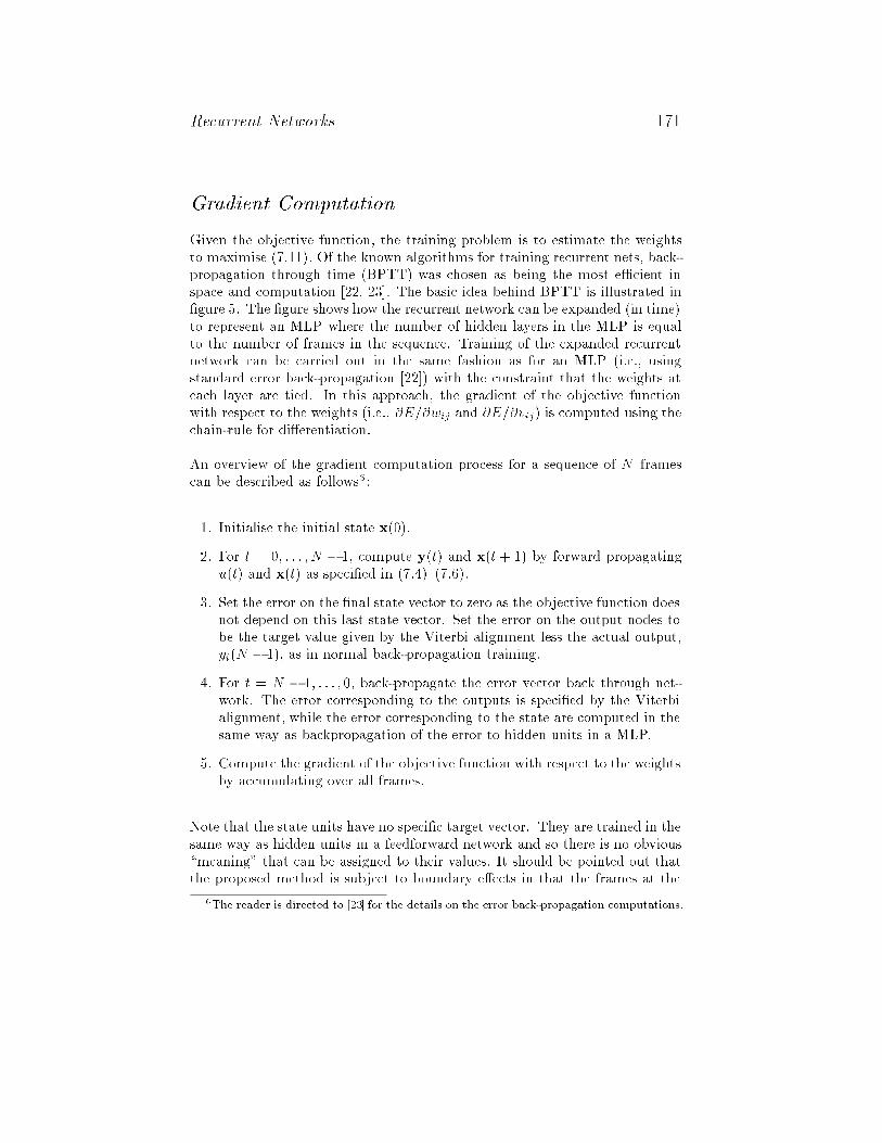
Given the objective function, the training problem is to estimate the weightsto maximise (7.11). Of the known algorithms for training recurrent nets, back-propagation through time (BPTT) was chosen as being the most e�cient inspace and computation [22, 23]. The basic idea behind BPTT is illustrated in�gure 5. The �gure shows how the recurrent network can be expanded (in time)to represent an MLP where the number of hidden layers in the MLP is equalto the number of frames in the sequence. Training of the expanded recurrentnetwork can be carried out in the same fashion as for an MLP (i.e., usingstandard error back-propagation [22]) with the constraint that the weights ateach layer are tied. In this approach, the gradient of the objective functionwith respect to the weights (i.e., and ) is computed using thechain-rule for di�erentiation.

An overview of the gradient computation process for a sequence of framescan be described as follows :

1. Initialise the initial state (0).

2. For = 0 1, compute ( ) and ( + 1) by forward propagating( ) and ( ) as speci�ed in (7.4){(7.6).

3. Set the error on the �nal state vector to zero as the objective function doesnot depend on this last state vector. Set the error on the output nodes tobe the target value given by the Viterbi alignment less the actual output,( 1), as in normal back-propagation training.

4. For = 1 0, back-propagate the error vector back through net-work. The error corresponding to the outputs is speci�ed by the Viterbialignment, while the error corresponding to the state are computed in thesame way as backpropagation of the error to hidden units in a MLP.

5. Compute the gradient of the objective function with respect to the weightsby accumulating over all frames.

Note that the state units have no speci�c target vector. They are trained in thesame way as hidden units in a feedforward network and so there is no obvious\meaning" that can be assigned to their values. It should be pointed out thatthe proposed method is subject to boundary e�ects in that the frames at the

@E=@w @E=@v

N

t ; : : : ; N t tu t t

y N

t N ; : : : ;

�

�

�

x

y x

x


Gradient Computation

u(0)

x(0)

u(N-1)

x(N)

u(1)

x(1) x(2) x(N-1)

y(0) y(1) y(N-1)

( )

( )

n

n

ij

7

7

( ) ( )

( )

( +1)( ) ( )

( ) ( )

( )

( )( )

( 1)

( 1)( )

( )

( )

( )

(0) ( )

( ) ( ) ( ) (0) 2

n nij

nij

nij

nij

nij

@E

@W

nij

nij

n

nij

nn

nij

nn

nij

n

n n= N

�

�

1

1 1 �

The expanded recurrent network.

The term is relative to neural networks, not standard HMM acoustic modellingtechniques.

large

end of a bu�er do not receive an error signal from beyond the bu�er. Althoughmethods exist to eliminate these e�ects (e.g., [23]), in practice it is found thatthe length of the expansion (typically 256 frames) is such that the e�ects areinconsequential.

There are a number of ways in which the gradient signal can be employed tooptimise the network. The approach described here has been found to be themost e�ective in estimating the large number of parameters of the recurrent

network. On each update, a local gradient, , is computed fromthe training frames in the th subset of the training data. A positive step

size, � , is maintained for every weight and each weight is adjusted by thisamount in the direction of the smoothed local gradient, i.e.,

=+ � if 0

� otherwise(7.12)

The local gradient is smoothed using a \momentum" term by

~=

~+ (1 ) (7.13)

The smoothing parameter, , is automatically increased from an initial valueof = 1 2 to = 1 1 by

= ( ) (7.14)

@E =@Wn

W

WW W >

W W:

@E

@W�

@E

@W�

@E

@W:

�� = � =N

� � � � e

�

�

�

� �

172

8<:

Weight Update

Chapter 7

Figure 5

( 1)

( 1)

( )

( )

n

n

ij

n

n

ij

�

�( +1)

( ) ~

1 ( )

nij

nij

@E

@W

@E

@W

�nij

where is the number of weight updates per pass through the training data.The step size is geometrically increased by a factor if the sign of the local gra-dient is in agreement with the averaged gradient, otherwise it is geometricallydecreased by a factor 1 , i.e.,

� =� if 0

� otherwise(7.15)

In this way, random gradients produce little overall change.

This approach is similar to the method proposed by Jacobs [24] except thata stochastic gradient signal is used and both the increase and decrease in thescaling factor is geometric (as opposed to an arithmetic increase and geometricdecrease). Considerable e�ort was expended in developing this training pro-cedure and the result was found to give better performance than the othermethods that can be found in the literature. Other surveys of \speed-up"techniques reached a similar conclusion [25, 26].

The recurrent network structure applied within the HMM framework providesa powerful model of the acoustic signal. Besides the obvious advantages ofincreased temporal context modelling capability and minimal assumptions onthe observation distributions, there are a number of less apparent advantagesto this approach. Four such advantages are described in this section.

Connectionist model combination refers to the process of merging the outputsof two or more networks. The original motivation for model merging with thehybrid system came from analysis of the recurrent network. Unlike a standardHMM, the recurrent network structure is time asymmetric. Training a networkto recognise forward in time will result in di�erent dynamics than training torecognise backwards in time. As di�erent information is available to both pro-cesses, it seems reasonable that better modelling can be achieved by combiningboth information sources.

N�

=�

W� W >

W:


5 SPECIAL FEATURES

5.1 Connectionist Model Combination

8<:

=1

( )

( )

=1

( )

=1

( )

i

K

k

ki

ki

K

k

k

i

ii

i

i

K

k

ki

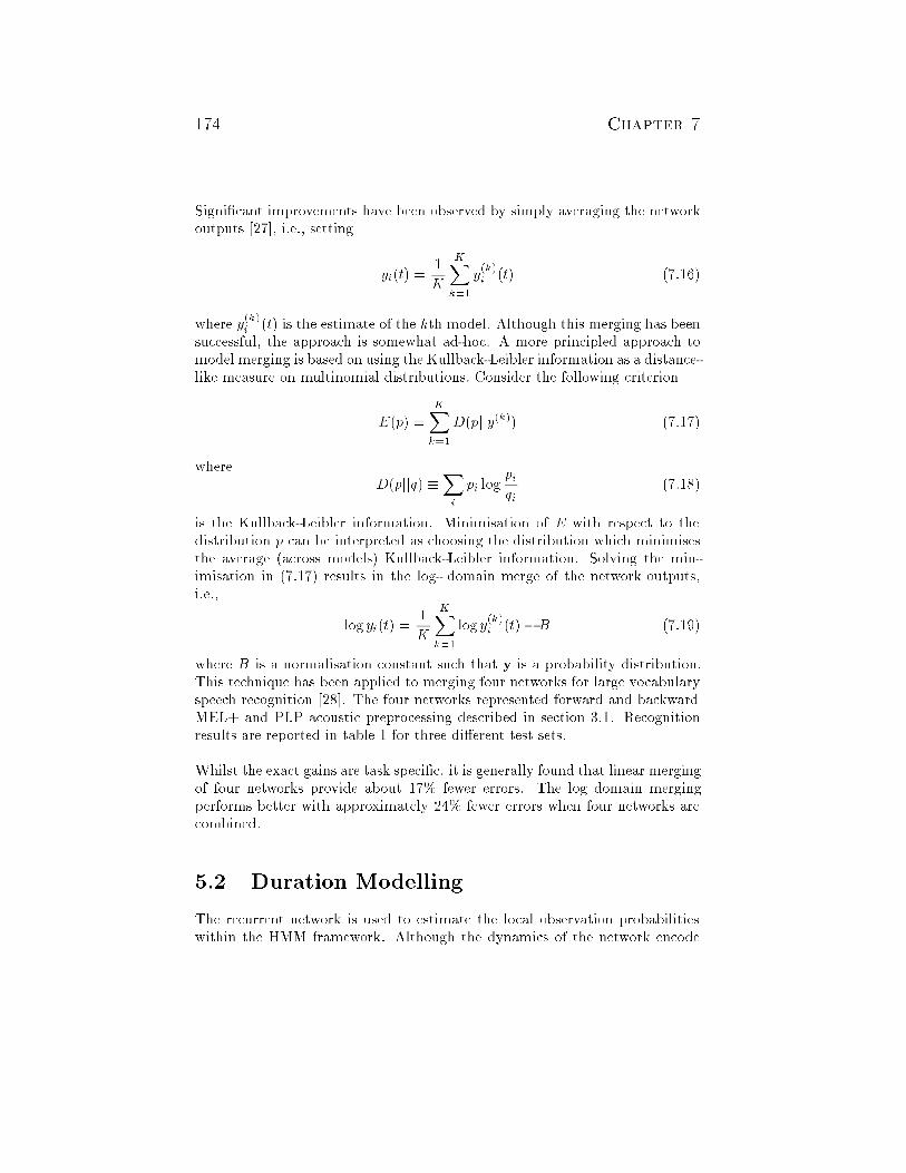
Signi�cant improvements have been observed by simply averaging the networkoutputs [27], i.e., setting

( ) =1

( ) (7.16)

where ( ) is the estimate of the th model. Although this merging has beensuccessful, the approach is somewhat ad-hoc. A more principled approach tomodel merging is based on using the Kullback-Leibler information as a distance-like measure on multinomial distributions. Consider the following criterion

( ) = ( ) (7.17)

where( ) log (7.18)

is the Kullback-Leibler information. Minimisation of with respect to thedistribution can be interpreted as choosing the distribution which minimisesthe average (across models) Kullback-Leibler information. Solving the min-imisation in (7.17) results in the log- domain merge of the network outputs,i.e.,

log ( ) =1

log ( ) (7.19)

where is a normalisation constant such that is a probability distribution.This technique has been applied to merging four networks for large vocabularyspeech recognition [28]. The four networks represented forward and backwardMEL+ and PLP acoustic preprocessing described in section 3.1. Recognitionresults are reported in table 1 for three di�erent test sets.

Whilst the exact gains are task speci�c, it is generally found that linear mergingof four networks provide about 17% fewer errors. The log domain mergingperforms better with approximately 24% fewer errors when four networks arecombined.

The recurrent network is used to estimate the local observation probabilitieswithin the HMM framework. Although the dynamics of the network encode

y tK

y t

y t k

E p D p y

D p q pp

q

Ep

y tK

y t B

B

jj

jj �

�

y

174

5.2 Duration Modelling

X

X

X

X

Chapter 7

8

8

1

t t

� N � N� �

Merging results for the ARPA 1993 spoke 5 development test, 1993spoke 6 development test, and the 1993 hub 2 evaluation test. All tests utiliseda 5,000 word vocabulary and a bigram language model and were trained usingthe SI-84 training set.

This is not necessarily the case for phone recognition where the network training criterionand the actual task are more closely linked.

Word Error Rate %Merge Type spoke 5 spoke 6 H2

17.3 15.0 16.217.1 15.1 16.517.8 15.5 16.116.9 14.4 15.217.3 15.0 16.015.2 11.4 13.413.4 11.0 12.6

some segmental information, explicit modelling of phone duration improves thehybrid system's performance on word recognition tasks .

Phone duration within the hybrid system is modelled with a hidden Markovprocess. In this approach, a Markov chain is used to represent phone dura-tion. The duration model is integrated into the hybrid system by expandingthe phone model from a single state to multiple states with tied observationdistributions, i.e.,

( = ) = ( = ) (7.20)

for and states of the same phone model.

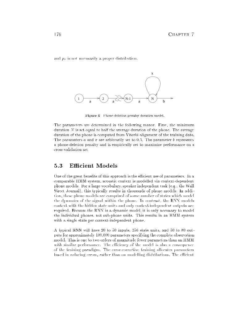
Choice of Markov chain topology is dependent on the decoding approach. De-coding using a maximum likelihood word sequence criterion is well suited tocomplex duration models as found in [29]. Viterbi decoding, however, resultsin a Markov chain on duration where the parameters are not hidden (given theduration). Because of this, a simple duration model as shown in �gure 6 isemployed. The free parameters in this model are (1) the minimum duration ofthe model, , (2) the value of the �rst 1 state transitions, , (3) the self-transition of the last state , and (4) the exit transition value, . The durationscore generated by this model is given as

=0 if

if(7.21)

p q i p q j

i j

N N ax b

p� < N;

a bx � N

j j

�

�

u u


�

Table 1

Forward Mel+

Forward PLP

Backward Mel+

Backward PLP

Average

Uniform Merge

Log-Domain

1 2 N-1 Na a a

x

b

�

Phone-deletion penalty duration model.

and is not necessarily a proper distribution.

The parameters are determined in the following manor. First, the minimumduration is set equal to half the average duration of the phone. The averageduration of the phone is computed from Viterbi alignment of the training data.The parameters and are arbitrarily set to 0 5. The parameter representsa phone-deletion penalty and is empirically set to maximise performance on across-validation set.

One of the great bene�ts of this approach is the e�cient use of parameters. In acomparable HMM system, acoustic context is modelled via context-dependentphone models. For a large vocabulary, speaker independent task (e.g., the WallStreet Journal), this typically results in thousands of phone models. In addi-tion, these phone models are comprised of some number of states which modelthe dynamics of the signal within the phone. In contrast, the RNN modelscontext with the hidden state units and only context-independent outputs arerequired. Because the RNN is a dynamic model, it is only necessary to modelthe individual phones, not sub-phone units. This results in an HMM systemwith a single state per context-independent phone.

A typical RNN will have 20 to 50 inputs, 256 state units, and 50 to 80 out-puts for approximately 100,000 parameters specifying the complete observationmodel. This is one to two orders of magnitude fewer parameters than an HMMwith similar performance. The e�ciency of the model is also a consequenceof the training paradigm. The error-corrective training allocates parametersbased in reducing errors, rather than on modelling distributions. The e�cient

p

N

a x : b

176

5.3 E�cient Models

Chapter 7

Figure 6

representation of the acoustic model results in a number of desirable properties,e.g., fast decoding.

The task of decoding is to �nd the maximum likelihood word sequence giventhe models and acoustic evidence. The time synchronous Viterbi algorithmprovides an e�cient means of performing this task for small vocabularies (e.g.,less than 1000 words) and short span language models (e.g., bigrams). However,with larger vocabularies and longer span language models a simple exhaustivesearch is not possible and the issue of e�cient decoding becomes critical to theperformance of the system.

A search procedure based on stack decoding [30, 31] has been adopted. Thissearch procedure may be regarded as a reordered time-synchronous Viterbidecoding and has the advantage that the language model is decoupled fromthe search procedure. Unlike time-synchronous Viterbi decoding, the Markovassumption is not integral to the search algorithm. Thus, this decoder architec-ture o�ers a exible platform for single-pass decoding using arbitrary languagemodels. The operation of the algorithm is described in some detail in [32, 33].Discussed below are some new approaches to pruning that have been developedto take advantage of hybrid system properties.

Two basic pruning criteria are used to reduce the computation required in de-coding. based pruning is similar to the various types of pruningused in most decoders and is based on the acoustic model likelihoods.

based pruning is speci�c to systems which employ a local posterior phoneprobability estimator.

Likelihood based methods are used to compute the envelope and also to set amaximum stack size. These rely on the computation of an estimate of the leastupper bound of the log likelihood at time t, . This is an updated estimateand is equal to the log likelihood of the most probable partial hypothesis attime . The size of the envelope is set heuristically and is dependent on theaccuracy of the estimate of . The second pruning parameter is used

t

Likelihood

Poste-

rior

lub(t)

lub(t)


5.4 Decoding

Search Algorithm

Pruning

Decoding performance on the Wall Street Journal task using a 20,000word vocabulary and a trigram language model. Accuracy and CPU time (inmultiples of realtime on an HP735) are given with respect to varying the like-lihood envelope and the posterior-based phone deactivation pruning threshold.The maximum stack size was set to be 31.

to control the maximum number of hypotheses in a stack. This parametermay be regarded as adaptively tightening the envelope, while ensuring thathypotheses are still extended at each time (subject to the overall envelope).

A second pruning method has been developed to take advantage of the connec-tionist probability estimator used in the hybrid system. The phone posteriorsmay be regarded as a local estimate of the presence of a phone at a particu-lar time frame. If the posterior probability estimate of a phone given a frameof acoustic data is below a threshold, then all words containing that phoneat that time frame may be pruned. This may be e�ciently achieved usinga tree organisation of the pronunciation dictionary. This process is referredto as . The posterior probability threshold used tomake the pruning decision may be empirically determined in advance using adevelopment set and is constant for all phones.

This posterior-based approach is similar to the likelihood-based channel-bankapproach of Gopalakrishnan et al. [34], which used phone-dependent thresholds.However, that system incurred a 5{10% relative search error to obtain a factorof two speedup on large vocabulary task. This new approach is extremely e�ec-tive. On a 20K trigram Wall Street Journal task, phone deactivation pruningcan result in close to an order of magnitude faster decoding, with less than 2%relative search error (see table 2).

20K Trigram, Trained on SI-84Pruning Parameters si dt s5 Nov '92Envelope Threshold Time %Error Time %Error

10 0.000075 16.1 12.1 15.7 12.610 0.0005 4.3 12.2 3.9 12.910 0.003 1.4 14.3 1.3 14.98 0.0 46.8 12.5 50.4 12.68 0.000075 5.4 12.2 4.9 12.88 0.0005 1.7 12.6 1.5 13.68 0.003 0.6 15.0 0.6 15.8

M

phone deactivation pruning

178 Chapter 7

Table 2

This section provides a concise description of the di�erences between the hy-brid RNN/HMM and standard HMM approaches. It should be pointed out thatmany of the capabilities attributed to the recurrent network can also be rep-resented by standard HMMs. However, the incorporation of these capabilitiesinto standard HMMs is not necessarily straightforward.

The parameters of the recurrent network are estimated with a discriminativetraining criterion. This leads to a mechanism for estimation of the posteriorprobability for the phones given the data. Standard HMM training utilises amaximum likelihood criterion for estimation of the phone model parameters.The recurrent network requires substantially fewer parameters because discrim-inative training focuses the model resources on decision boundaries instead ofmodeling the complete class likelihoods.

One of the main bene�ts of the recurrent network is that it relaxes the con-ditional independence assumption for the local observation probabilities. Thisresults in a model which can represent the acoustic context without explic-itly modeling phonetic context. This has positive rami�cations in terms of thenumber of required parameters and the complexity of the search procedure.

The second main assumption of standard HMMs is that the observation distri-butions are from the exponential family (e.g., multinomial, Gaussian, etc.) ormixtures of exponential family distributions. The recurrent network, however,makes much fewer assumptions about the form of the acoustic vector distribu-tion. In fact, it is quite straightforward to use real-valued and/or categoricaldata for the acoustic input. In theory, a Gaussian mixture distribution and arecurrent network can both be considered nonparametric estimators by allow-ing the size (e.g., number of mixtures or state units, respectively) to increasewith additional training data. However, because standard HMMs employ max-imum likelihood estimation there is the practical problem of su�cient data toestimate all the parameters. Because the recurrent network shares the stateunits for all phones, this data requirement is less severe.


6 SUMMARY OF VARIATIONS

6.1 Training Criterion

6.2 Distribution Assumptions

There are a number of practical advantages to the use of a recurrent network in-stead of an exponential family distribution. The �rst, mentioned in section 6.1,is that the number of required parameters is much fewer than standard sys-tems. In addition, section 5.4 shows that the posterior probabilities generatedby the network can be used e�ciently in the decoding { both for computinglikelihoods and pruning state paths (similar to fast-match approaches whichare add-ons to standard systems). Of course, a major practical attraction ofthe approach is that it is very straightforward to map the recurrent network tostandard DSP architectures.

A hybrid RNN/HMM system has been applied to an open vocabulary task;namely the 1993 ARPA evaluation of continuous speech recognition systems.The hybrid system employed context-independent phone models for a 20,000word vocabulary with a backed-o� trigram language model. Forward and back-ward in time and recurrent networks were merged to generate theobservation probabilities. The performance of this simple system (17% worderror rate using less than a half million parameters for acoustic modelling) wassimilar to that of much larger, state-of-the-art HMM systems. This system hasrecently been extended to a 65,533 word vocabulary and the simplicity of thehybrid approach resulted in decoding with minimal search errors in only 2.5minutes per sentence.

Recurrent networks are able to model speech as well as standard techniquessuch as hidden Markov models based on Gaussian mixture densities. Recur-rent networks di�er from the HMM approach in making fewer assumptions onthe distributions of the acoustic vectors, having a means of incorporating longterm context, using discriminative training, and providing a compact set ofphoneme probabilities which may be e�ciently searched for large vocabularyrecognition. There are also practical di�erences such as the fact that the train-ing of the systems is slower than the HMM counterpart, but this is made up forby faster execution at recognition time. The RNN system also has relatively

MEL+ PLP

180

6.3 Practical Issues

7 A LARGE VOCABULARY SYSTEM

8 CONCLUSION

Chapter 7

few parameters, and these are used in a simple multiply and accumulate loop sohardware implementation is more plausible. In summary, recurrent networksare an attractive, alternative statistical model for use in the core of a largevocabulary recognition system.

Two of the authors, T.R. and S.R., held U. K. Engineering and Physical Sci-ences Research Council Fellowships. This work was supported in part by ES-PRIT project 6487, WERNICKE. For the reported experiments, the pronunci-ation dictionaries were provided by Dragon Systems and the language modelswere provided by MIT Lincoln laboratories.

[1] H. F. Silverman and D. P. Morgan, \The application of dynamic pro-gramming to connected speech recognition," , vol. 7,pp. 6{25, July 1990.

[2] L. R. Rabiner, \A tutorial on hidden Markov models and selected applica-tions in speech recognition," , vol. 77, pp. 257{286,February 1989.

[3] N. Morgan and H. Bourlard, \Continuous speech recognition using multi-layer perceptrons with hidden Markov models," in , pp. 413{416, 1990.

[4] S. Renals, N. Morgan, H. Bourlard, M. Cohen, and H. Franco, \Connec-tionist probability estimators in HMM speech recognition,"

, vol. 2, Jan. 1994.

[5] F. Jelinek and R. Mercer, \Interpolated estimation of Markov source pa-rameters from sparse data," , pp. 381{397,1980.

[6] K.-F. Lee,. Boston: Kluwer Academic Publishers, 1989.

IEEE ASSP Magazine

Proceedings of the IEEE

Proc. ICASSP

IEEE Trans-

actions on Speech and Audio Processing

Pattern Recognition in Practice

Automatic Speech Recognition: The Development of the

SPHINX System


Acknowledgements

REFERENCES

[7] S. Furui, \Speaker-independent isolated word recognition using dynamicfeatures of speech spectrum,"

, vol. 34, pp. 52{59, Feb. 1986.

[8] E. B. Baum and F. Wilczek, \Supervised learning of probability distri-butions by neural networks," in(D. Z. Anderson, ed.), American Institute of Physics, 1988.

[9] J. S. Bridle, \Probabilistic interpretation of feedforward classi�ca-tion network outputs, with relationships to statistical pattern recogni-tion," in(F. Fougelman-Soulie and J. He�rault, eds.), pp. 227{236, Springer-Verlag,1989.

[10] H. Bourlard and C. J. Wellekens, \Links between Markov models and mul-tilayer perceptrons,"

, vol. 12, pp. 1167{1178, Dec. 1990.

[11] H. Gish, \A probabilistic approach to the understanding and training ofneural network classi�ers," in , pp. 1361{1364, 1990.

[12] M. D. Richard and R. P. Lippmann, \Neural network classi�ers estimateBayesian a posteriori probabilities," , vol. 3, pp. 461{483, 1991.

[13] H. Bourlard and N. Morgan,. Kluwer Academic Publishers, 1994.

[14] J. S. Bridle, \ALPHA-NETS: A recurrent `neural' network architecturewith a hidden Markov model interpretation," ,vol. 9, pp. 83{92, Feb. 1990.

[15] J. S. Bridle and L. Dodd, \An Alphanet approach to optimising inputtransformations for continuous speech recognition," in ,pp. 277{280, 1991.

[16] L. T. Niles and H. F. Silverman, \Combining hidden Markov models andneural network classi�ers," in , pp. 417{420, 1990.

[17] S. J. Young, \Competitive training in hidden Markov models," in, pp. 681{684, 1990. Expanded in the technical report CUED/F-

INFENG/TR.41, Cambridge University Engineering Department.

[18] A. J. Robinson and F. Fallside, \Static and dynamic error propagationnetworks with application to speech coding," in

(D. Z. Anderson, ed.), American Institute of Physics, 1988.

IEEE Transactions on Acoustics, Speech,

and Signal Processing

Neural Information Processing Systems

Neuro-computing: Algorithms, Architectures and Applications

IEEE Transactions on Pattern Analysis and Machine

Intelligence

Proc. ICASSP

Neural Computation

Continuous Speech Recognition: A Hybrid

Approach

Speech Communication

Proc. ICASSP

Proc. ICASSP

Proc.

ICASSP

Neural Information Pro-

cessing Systems

182 Chapter 7

[19] P. McCullagh and J. A. Nelder, . London: Chap-man and Hall, 1983.

[20] T. Robinson, \The state space and \ideal input" representations of recur-rent networks," in , pp. 327{334,John Wiley and Sons, 1993.

[21] A. P. Dempster, N. M. Laird, and D. B. Rubin, \Maximum likelihood fromincomplete data via the EM algorithm (with discussion),"

, vol. B39, pp. 1{38, 1977.

[22] D. E. Rumelhart, G. E. Hinton, and R. J. Williams, \Learning internal rep-resentations by error propagation," in

(D. E.Rumelhart and J. L. McClelland, eds.), ch. 8, Cambridge, MA: BradfordBooks/MIT Press, 1986.

[23] P. J. Werbos, \Backpropagation through time: What it does and how todo it," , vol. 78, pp. 1550{1560, Oct. 1990.

[24] R. A. Jacobs, \Increased rates of convergence through learning rate adap-tation," , vol. 1, pp. 295{307, 1988.

[25] W. Schi�mann, M. Joost, and R. Werner, \Optimization of the backprop-agation algorithm for training multilayer perceptrons," tech. rep., Univer-sity of Koblenz, 1992.

[26] T. T. Jervis and W. J. Fitzgerald, \Optimization schemes for neural net-works," Tech. Rep. CUED/F-INFENG/TR144, Cambridge University En-gineering Department, Aug. 1993.

[27] M. M. Hochberg, S. J. Renals, A. J. Robinson, and D. J. Kershaw, \Largevocabulary continuous speech recognition using a hybrid connectionist-HMM system," in , pp. 1499{1502, 1994.

[28] M. M. Hochberg, G. D. Cook, S. J. Renals, and A. J. Robinson, \Con-nectionist model combination for large vocabulary speech recognition," in

(J. Vlontzos, J.-N. Hwang, andE. Wilson, eds.), pp. 269{278, IEEE, 1994.

[29] T. H. Crystal and A. S. House, \Segmental durations in connected-speechsignals: Current results," , vol. 83, pp. 1553{1573, Apr.1988.

Generalised Linear Models

Visual Representations of Speech Signals

J. Roy. Statist.

Soc.

Parallel Distributed Processing: Ex-

plorations in the Microstructure of Cognition. Vol. I: Foundations.

Proc. IEEE

Neural Networks

Proc. of ICSLP-94

Neural Networks for Signal Processing IV

J. Acoust. Soc. Am.


[30] L. R. Bahl and F. Jelinek, \Apparatus and method for determining a likelyword sequence from labels generated by an acoustic processor." US Patent4,748,670, May 1988.

[31] D. B. Paul, \An e�cient A* stack decoder algorithm for continuous speechrecognition with a stochastic language model," in , vol. 1,(San Francisco), pp. 25{28, 1992.

[32] S. J. Renals and M. M. Hochberg, \Decoder technology for con-nectionist large vocabulary speech recognition," Tech. Rep. CUED/F-INFENG/TR.186, Cambridge University Engineering Department, 1994.

[33] S. Renals and M. Hochberg, \E�cient search using posterior phone prob-ability estimates," in , pp. 596{599, 1995.

[34] P. S. Gopalakrishnan, D. Nahamoo, M. Padmanabhan, and M. A. Picheny,\A channel-bank-based phone detection strategy," in , vol. 2,(Adelaide), pp. 161{164, 1994.

Proc. ICASSP

Proc. ICASSP

Proc. ICASSP

184 Chapter 7

THE USE OF RECURRENT NEURAL NETWORKS IN CONTINUOUS …

Documents

Transcript of THE USE OF RECURRENT NEURAL NETWORKS IN CONTINUOUS …