The Use of Rasch Modeling To Improve Standard Setting

Practical Assessment, Research, and Evaluation Practical Assessment, Research, and Evaluation

Volume 11 Volume 11, 2006 Article 2

2006

The Use of Rasch Modeling To Improve Standard Setting The Use of Rasch Modeling To Improve Standard Setting

Robert G. MacCann

Gordon Stanley

Follow this and additional works at: https://scholarworks.umass.edu/pare

Recommended Citation Recommended Citation MacCann, Robert G. and Stanley, Gordon (2006) "The Use of Rasch Modeling To Improve Standard Setting," Practical Assessment, Research, and Evaluation: Vol. 11 , Article 2. DOI: https://doi.org/10.7275/sbnk-w656 Available at: https://scholarworks.umass.edu/pare/vol11/iss1/2

This Article is brought to you for free and open access by ScholarWorks@UMass Amherst. It has been accepted for inclusion in Practical Assessment, Research, and Evaluation by an authorized editor of ScholarWorks@UMass Amherst. For more information, please contact [email protected].

https://scholarworks.umass.edu/pare

https://scholarworks.umass.edu/pare/vol11

https://scholarworks.umass.edu/pare/vol11/iss1/2

https://scholarworks.umass.edu/pare?utm_source=scholarworks.umass.edu%2Fpare%2Fvol11%2Fiss1%2F2&utm_medium=PDF&utm_campaign=PDFCoverPages

https://scholarworks.umass.edu/pare/vol11/iss1/2?utm_source=scholarworks.umass.edu%2Fpare%2Fvol11%2Fiss1%2F2&utm_medium=PDF&utm_campaign=PDFCoverPages

mailto:[email protected]

A peer-reviewed electronic journal.

Copyright is retained by the first or sole author, who grants right of first publication to the Practical Assessment, Research & Evaluation. Permission is granted to distribute this article for nonprofit, educational purposes if it is copied in its entirety and the journal is credited.

Volume 11 Number 2, January 2006 ISSN 1531-7714

The Use of Rasch Modeling To Improve Standard Setting Robert G. MacCann and Gordon Stanley Board of Studies, NSW Australia

This paper examines four ways in which Rasch modeling may be used to improve standard setting. The first three methods are applied to the Angoff procedure and the fourth is an example of bookmarking. Using an actual data set taken from the New South Wales School Certificate test in Mathematics, worked examples are provided that show how informative data may be provided to the judges, both before and after they Angoff-rate the test items. In addition, an example of bookmarking is given, along with a variant of the latter known as item mapping. The application of non Rasch IRT procedures to standard setting is also discussed.

Standard setting is now a fundamental goal for reporting educational outcomes in many education systems around the world. It is in widespread use across the US in state testing systems and is used in the UK. In Australia, it is used in all the Year 10 and Year 12 examinations in the New South Wales (NSW) education system (Board of Studies NSW, 2003). The two most popular procedures for standard setting are the Angoff method (Angoff, 1971) and a newer procedure, the Bookmark method (Mitzel, Lewis, Patz and Green, 2001).

Standard setting involves a systematic set of

procedures that identifies a common judgement as to the cut score required for a given level of proficiency. It would be naïve to think that such procedures identify a “true” standard which separates proficiency from non-proficiency. Standards are in an obvious sense arbitrary, being influenced by the perceived characteristics of the examinees, the educational experiences and values of the particular judges and the expectations of the society from which the judges are drawn. The arbitrary nature of standards, however, does not

mean they are capricious, and does not negate the educational benefits that may flow from their establishment. The most important requirement of such standard-setting procedures is that of consistency—once consensus among the judges is reached, the procedures should classify the same type of students as being proficient across different occasions, test instruments, judging panels and so on.

While the Angoff method was originally

conceived as a one-stage test-centered process, it has now typically developed into a multi-stage procedure in which the judges make independent judgements and then discuss their initial decisions. This group discussion process has been advocated by several researchers (for example, Jaeger, 1982; Norcini, Lipner, Langdon and Strecker, 1987; Morrison, Busch and D’Arcy, 1994; Berk, 1996). In the discussion phase it is customary to provide the judges with data on the accuracy of their initial decisions. Providing the judges with such data has been suggested by Popham (1978), Linn (1978), Cross, Impara, Frary and Jaeger (1984), and

1

MacCann and Stanley: The Use of Rasch Modeling To Improve Standard Setting

Published by ScholarWorks@UMass Amherst, 2006

Practical Assessment Research & Evaluation, Vol. 11, No. 2 2 MacCann & Stanley, Rasch Standard Setting Norcini, Shea and Kanya (1988). There is a natural affinity between IRT models and many standard-setting procedures, with a shared view of a continuum of achievement and a probabilistic definition of mastery on an item. Both van der Linden (1982) and Kane (1987) have discussed the similarities between IRT models and Angoff standard-setting procedures.

Given that standard setting in certification has

high stakes for individuals, there is considerable interest in understanding the process and in finding ways to reduce variability in standard setting from occasion to occasion (MacCann and Stanley, 2004). Using a data set taken from a state-wide standard-setting operation, this paper will illustrate some ways in which Item Response Theory (IRT) can be used to provide feedback to help judges in both the Angoff and Bookmarking procedures.

THE SCHOOL CERTIFICATE MATHEMATICS PROGRAM

To show the ways in which Rasch modeling can

be used to improve standard setting, data based on a multi-stage Angoff procedure will be analysed. The test comprised 50 short items, which were dichotomously scored—0 for a wrong answer, 1 for the correct answer. The test items came from the School Certificate Mathematics external test program, which tests the fundamental knowledge and skills of students in Year 10 in New South Wales (generally of age 15-16 years). Approximately 78,000 students attempt this compulsory test, but the analyses below were based on a simple random sample of 10,000 students. This program uses a three-stage Angoff procedure with six experienced teacher-judges to allocate each student to one of six performance bands. The highest band, Band 6, which generally corresponds to the top 3-10% of students, will be used for the purposes of illustration in this paper.

ITEM RESPONSE THEORY IRT developed from the initial work of Lord

(1952, 1953) on latent trait models and the independent development by Rasch of the one-

parameter model (Rasch, 1960, 1966). In contrast to Classical Test Theory (CTT), IRT uses relatively strong assumptions but produces a measurement scale that has a number of advantages over CTT and now holds a central place in educational measurement theory. For expositions of IRT and the various models that have been developed see Lord (1980), Hambleton, Swaminathan and Rogers (1991), van der Linden and Hambleton (1997), Embretson and Reise (2000).

In the NSW education system, the one-

parameter Rasch model is widely used to analyse tests. The Rasch model software package employed in this paper is RUMM—Rasch Unidimensional Measurement Models (Andrich, Sheridan, Lyne and Luo, 2000). The Rasch model is the simplest of the IRT models, having only one parameter to describe an item—its difficulty. In addition, each person has one parameter to describe their performance—their ability.

The RUMM software accepts the usual type of

data file where the student records are in rows and the test items are in columns. Applying the appropriate mathematical modeling to this data matrix, the software produces a person ability estimate for each student, and an item difficulty estimate for a test item. These estimates are on the logit scale (log odds units), a scale arbitrarily centred on zero for the difficulty of the test items, and theoretically ranging from minus infinity to plus infinity. (In practice most estimates fall in the –4 to +4 range.)

The relationship between total score and ability in logits

For the case of all items being compulsory (as

they are in School Certificate Mathematics), and for the one parameter logistic model, the total score is a sufficient statistic for estimating a student’s ability level (Andersen, 1973). This implies that every examinee on the same total score will receive the same ability estimate. The relationship between the total score and the ability estimate is shown below in Figure 1.

2

Practical Assessment, Research, and Evaluation, Vol. 11 [2006], Art. 2

https://scholarworks.umass.edu/pare/vol11/iss1/2DOI: https://doi.org/10.7275/sbnk-w656

Practical Assessment Research & Evaluation, Vol. 11, No. 2 3 MacCann & Stanley, Rasch Standard Setting

-5

-4

-3

-2

-1

0

1

2

3

4

5

6

0 5 10 15 20 25 30 35 40 45

Total score

Abi

lity

(logi

ts)

Figure 1: Conversion from total score to ability in logits

A conversion table like this should be obtainable from all reputable Rasch software packages. Note that the conversion is relatively linear for a large part of the mark range, but increases sharply in the upper mark range. A few marks total score difference in the upper mark range results in a larger ability difference than would occur for the same total score difference near the middle of the distribution. Similarly, the conversion decreases sharply at the bottom of the mark range. For students scoring full marks (50), or zero marks, ability estimates are hard to justify, although some software packages give such estimates.

This conversion between total score and ability

(and vice versa) is frequently used in the procedures to follow.

ANGOFF PROCEDURES

In the Angoff method, a panel of judges is

assembled which is representative of the community that works with and interprets the standards. In the NSW system, this comprises six experienced teachers. For the traditional Angoff method, each judge works through the test items independently, estimating the probability of success on each item for the candidates under consideration. In practice, rather than express the task in terms of

probabilities, the judges are usually asked to envisage a group of such candidates and to estimate the proportion of the group who would succeed on the item. This results in a series of Angoff-ratings for each judge. When these ratings are regarded as final, they are summed over all the items in the test to produce a total cut score for the judge. A final total cut score is obtained by averaging across the judges’ total cut scores. This is the Angoff method in its basic state.

This basic procedure has typically evolved into a

multi-staged process in most systems. Whereas the judges work independently in the first stage described above, in the later stages the judges usually collaborate and receive some form of feedback on the accuracy of their judgements. Thus, the judges usually get to modify their judgements before they become final and are summed over items and averaged across judges. In addition, material is often provided to help the judges formulate an image of the desired candidates who are proficient at the given level. For example, if the system has been in operation for some years, “Standards Packages” on CD-Rom may be made available for the judges to study. These typically contain test items from previous years showing the success rates obtained by candidates near the total cut score.

3




In the sections below, it will be shown how

Rasch modeling can assist the judges in forming and modifying their Angoff-ratings.

Data which assists the judges to make item probability estimates

This section deals with the Angoff procedures

and illustrates the type of information that could be given to the judges before they give Angoff probability ratings to each item. Firstly, the test is analysed via IRT to produce item difficulty estimates and person ability estimates. The relationship between a total score on the 50 items and person ability is given in Figure 1. From this figure, given a total score, an ability can be determined. Then given the person ability and the difficulty of the item, the probability of success on item j by person i is given by

)(1

1jie

Pij βθ −−+= . (1)

where iθ is the ability of person i, and jβ is the

difficulty of item j. (Note that there are other forms of this

equation. For example, it is sometimes written

)(1

1jiaDij

eP

βθ ′−′−+= ,

where D is a scaling constant, a is a common

level of discrimination for all items and their product may be termed the scaling factor. By letting

ii aD θθ ′= and jj aD ββ ′= , the scaling factor is absorbed into the ability and difficulty scale to create the simpler form of Equation 1.)

From Equation 1 a table can be generated

which shows how students on a particular total score would be expected to perform on each item, as in Table 1 below. This table could be provided

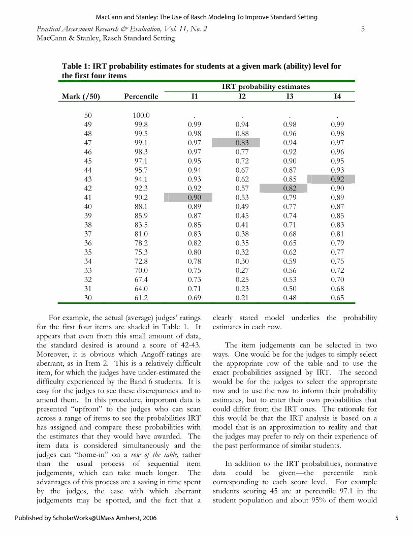
to the judges before they attempt their Angoff ratings. To save space, it is shown here for a range of total scores surrounding the expected cut score and only for the first four items in the test. It gives the probability that students at a given score level would correctly answer the item. No probability estimates are given for a perfect score of 50 as this represents a ceiling that may distort the value of any attempted estimate.

For example, according to the IRT model, of

the students scoring 45 (/50) on the total test, about 95% would be expected to be correct on Item 1, but only 72% would be expected to be correct on Item 2. In addition to providing information of students’ expected performance on an item, this also provides a means of comparing the difficulty of the items at different ability levels. Clearly Item 2 is generally a much more difficult item than Item 1.

Comparing Item 1 with Item 3 gives little

difference in the probability levels for students on a score of 47 (97% versus 94%), but this difference increases at lower ability levels. For example, for students on a score of 42, 92% are predicted to be correct on Item 1 but only 82% on Item 3.

In the approach considered here, Table 1 would

be presented “upfront” to the judges. They would scan the Item 1 probability column and encircle the probability that best matched their Angoff-rating for Item 1. They would repeat this process for several items. If the encircled probabilities tended to fall on the same row, then they could stop when they were satisfied that the row reflected the standard of which they are thinking. Some judges may need only a small number of comparisons before settling on a row, while others may need to cover most of the items before then choosing the row that best fits the pattern of encircled probabilities. Once a row is tentatively chosen, the remaining items can be dealt with more quickly, as a confirmatory check, rather than performing Angoff ratings in isolation.

4




Table 1: IRT probability estimates for students at a given mark (ability) level for the first four items

IRT probability estimates Mark (/50) Percentile I1 I2 I3 I4

50 100.0 . . . . 49 99.8 0.99 0.94 0.98 0.99 48 99.5 0.98 0.88 0.96 0.98 47 99.1 0.97 0.83 0.94 0.97 46 98.3 0.97 0.77 0.92 0.96 45 97.1 0.95 0.72 0.90 0.95 44 95.7 0.94 0.67 0.87 0.93 43 94.1 0.93 0.62 0.85 0.92 42 92.3 0.92 0.57 0.82 0.90 41 90.2 0.90 0.53 0.79 0.89 40 88.1 0.89 0.49 0.77 0.87 39 85.9 0.87 0.45 0.74 0.85 38 83.5 0.85 0.41 0.71 0.83 37 81.0 0.83 0.38 0.68 0.81 36 78.2 0.82 0.35 0.65 0.79 35 75.3 0.80 0.32 0.62 0.77 34 72.8 0.78 0.30 0.59 0.75 33 70.0 0.75 0.27 0.56 0.72 32 67.4 0.73 0.25 0.53 0.70 31 64.0 0.71 0.23 0.50 0.68 30 61.2 0.69 0.21 0.48 0.65

For example, the actual (average) judges’ ratings

for the first four items are shaded in Table 1. It appears that even from this small amount of data, the standard desired is around a score of 42-43. Moreover, it is obvious which Angoff-ratings are aberrant, as in Item 2. This is a relatively difficult item, for which the judges have under-estimated the difficulty experienced by the Band 6 students. It is easy for the judges to see these discrepancies and to amend them. In this procedure, important data is presented “upfront” to the judges who can scan across a range of items to see the probabilities IRT has assigned and compare these probabilities with the estimates that they would have awarded. The item data is considered simultaneously and the judges can “home-in” on a row of the table, rather than the usual process of sequential item judgements, which can take much longer. The advantages of this process are a saving in time spent by the judges, the ease with which aberrant judgements may be spotted, and the fact that a

clearly stated model underlies the probability estimates in each row.

The item judgements can be selected in two

ways. One would be for the judges to simply select the appropriate row of the table and to use the exact probabilities assigned by IRT. The second would be for the judges to select the appropriate row and to use the row to inform their probability estimates, but to enter their own probabilities that could differ from the IRT ones. The rationale for this would be that the IRT analysis is based on a model that is an approximation to reality and that the judges may prefer to rely on their experience of the past performance of similar students.

In addition to the IRT probabilities, normative

data could be given—the percentile rank corresponding to each score level. For example students scoring 45 are at percentile 97.1 in the student population and about 95% of them would

5



Practical Assessment Research & Evaluation, Vol. 11, No. 2 6 MacCann & Stanley, Rasch Standard Setting be expected to be correct on Q1 but only 72% on Q2, according to the IRT model. Such a table could be presented without the column giving the percentile rank. Reid (1991) has argued that the use of normative data in standards-setting needs to be carefully handled. Once the judges see the normative data, it may prove to be a dominant factor that biases the item judgements. On the other hand, Wiliam (1996) points out the danger that test-centered standards-setting procedures may lose touch with what students can actually do, resulting in set standards that are quite difficult to achieve. The total cut score equivalents of each item judgement

In this section, the judges have Angoff-rated

each item but have not yet summed the items to get a total cut score. Here feedback is given on the equivalent total cut score for each item. When the judges estimate a probability of success for an item, they are, in effect, setting an ability level. The item has a known difficulty level obtained from the IRT analysis and the judges are estimating a probability of success for cut score level type students. The estimated ability of the students at this cut score level is obtained by rearranging Equation 1 so that the person ability is a function of the probability of success on the item, giving:

⎟⎟⎠

⎞⎜⎜⎝

⎛ −−=

ij

ijji P

P1lnβθ . (2)

where ln is the natural logarithm (logarithm to the base e).

The person ability is then converted to an equivalent total score on the test by using a conversion table similar to that graphed in Figure 1. For example, an ability of 2 logits translates to an expected total score of 41.4. This allows the generation of Table 2 below, which shows the expected total cut scores for the first 25 items.

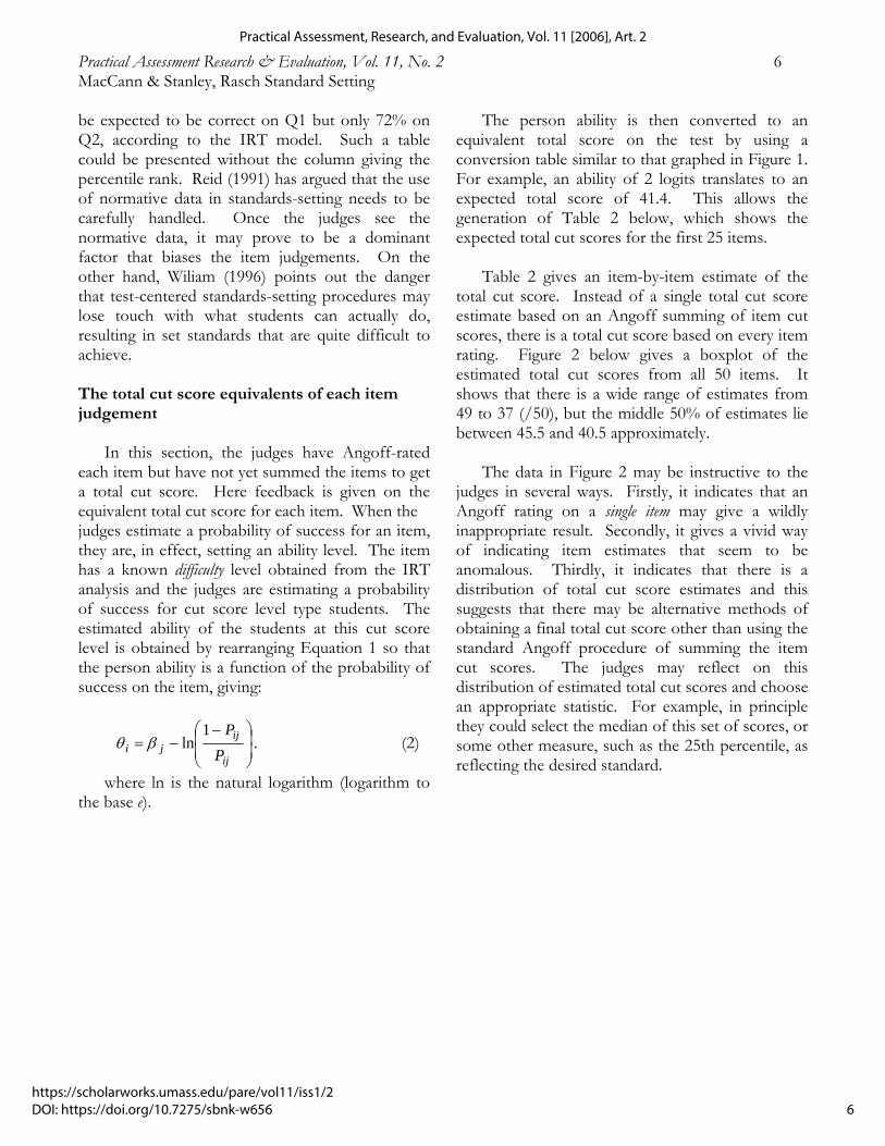
Table 2 gives an item-by-item estimate of the

total cut score. Instead of a single total cut score estimate based on an Angoff summing of item cut scores, there is a total cut score based on every item rating. Figure 2 below gives a boxplot of the estimated total cut scores from all 50 items. It shows that there is a wide range of estimates from 49 to 37 (/50), but the middle 50% of estimates lie between 45.5 and 40.5 approximately.

The data in Figure 2 may be instructive to the

judges in several ways. Firstly, it indicates that an Angoff rating on a single item may give a wildly inappropriate result. Secondly, it gives a vivid way of indicating item estimates that seem to be anomalous. Thirdly, it indicates that there is a distribution of total cut score estimates and this suggests that there may be alternative methods of obtaining a final total cut score other than using the standard Angoff procedure of summing the item cut scores. The judges may reflect on this distribution of estimated total cut scores and choose an appropriate statistic. For example, in principle they could select the median of this set of scores, or some other measure, such as the 25th percentile, as reflecting the desired standard.

6




Table 2: A total cut score estimate based on each item Item Judges’ Angoff

rating IRT ability matching

Angoff rating

Corresponding total cut score

1 0.91 2.005 41.4 2 0.82 3.315 46.8 3 0.83 2.133 42.1 4 0.92 2.329 43.1 5 0.98 2.731 44.9 6 0.64 2.863 45.4 7 0.76 1.902 40.8 8 0.87 1.523 38.4 9 0.83 2.750 45.0

10 0.99 4.268 48.6 11 0.73 3.243 46.6 12 0.85 3.437 47.1 13 0.85 2.742 45.0 14 0.91 1.606 38.9 15 0.87 2.644 44.6 16 0.90 4.639 49.0 17 0.73 2.573 44.3 18 0.78 3.351 46.9 19 0.99 3.490 47.3 20 0.98 3.340 46.9 21 0.94 1.593 38.9 22 0.99 1.963 41.2 23 0.96 2.278 42.9 24 0.98 3.342 46.9 25 0.97 2.182 42.4

50

49

48

47

46

45

44

43

42

41

40

39

38

37

3635

Figure 2: Boxplot of the estimated Total Cut Scores – each item providing a Cut Score

7



Practical Assessment Research & Evaluation, Vol. 11, No. 2 8 MacCann & Stanley, Rasch Standard Setting Feedback to the judges on the accuracy of their probability ratings

In the standard Angoff procedure, the item cut

scores are summed to give a total cut score. This total cut score can be converted into a person ability measure via a conversion table, as shown in Figure 1. In addition, an item difficulty estimate in logits is available for each item from the IRT analysis.

Then Equation 1 can be used to estimate the

probability of success on each item and compare it with the judges’ estimated probability of success (the Angoff rating). This is shown in Table 3 below for the first 30 items.

Such a table can be presented in item order (as

shown) above or sorted in order of the discrepancy between the IRT probability and the judges’ probability. The latter would clearly show the judges the items where their judgements were most discrepant from the results of the IRT model. Most Angoff procedures in recent times are multi-stage. This statistical feedback would give the judges a chance to rethink some of their ratings in the second stage. For example, Item 16 (shaded in the table) is a very difficult item according to the IRT analysis, with a difficulty rating of 2.44 logits. The predicted IRT probability of success was only 0.55 for the Band 6 marginal students on this item. However, the judges expected the high-level Band 6 students to perform well on the item, with an average probability of success rating of 0.90. This discrepancy is an indicator to the judges to closely re-examine this item and attempt to determine why it proved to be so difficult in general, and to the high ability Band 6 group, and to adjust their ratings accordingly.

BOOKMARKING PROCEDURES A newer method of standard setting which does

not involve item by item judgements is the Bookmark method (Mitzel et al, 2001). In this procedure the test is analysed by IRT to produce item difficulty estimates and person ability

estimates. A criterion probability is then set such that, for students conceived to be at the marginal cut score level, two-thirds of the group would be expected to succeed on the item. The task of the judges is to search through the test for this item—the one with a probability of success of 0.667 for students at the cut score. This probability is termed the response probability (RP) and is commonly set at two-thirds (Reckase, 2000; Mitzel et al., 2001; Buckendahl, Smith, Impara and Plake, 2002).

A second important concept is the bookmark

difficulty location (BDL). Given the difficulty of an item in logits and the response probability, one can determine the ability level required for a probability of success on an item equal to the response probability. This ability level is the BDL. Note that although this measure is called a difficulty location, it is defined as an ability level (the ability and difficulty being measured on the same scale). The BDL is calculated for each item, and is used to rank the items in order in a booklet starting from the lowest BDL (corresponding to easy items) to the highest BDL (corresponding to difficult items).

To calculate the BDL for the Rasch model, Equation 2 is used. Substituting the response probability (RP) gives the BDL for a particular item:

⎟⎠⎞

⎜⎝⎛ −

−=RP

RPBDL jj1lnβ . (3)

That is jjBDL β= + constant. For example, for a response probability of two-

thirds, putting RP = 2/3 in Equation 3 gives

69315.0+= jjBDL β . However, other response probabilities can be

used. Wang (2003) advocates a response probability of 0.5 which (substituting RP = 0.5 into Equation 3) gives

jjBDL β= , (4) with a constant of zero.

8




Table 3: Comparison of Judges’ and IRT probability estimates

Probability of being correct for ability at the

cut score Item IRT item

difficulty Judges’ estimate

IRT estimate Difference

1 -0.288 0.91 0.95 -0.040 2 1.821 0.82 0.69 0.125 3 0.582 0.83 0.89 -0.061 4 -0.136 0.92 0.94 -0.019 5 -1.161 0.98 0.98 0.002 6 2.280 0.64 0.59 0.055 7 0.758 0.76 0.87 -0.108 8 -0.349 0.87 0.95 -0.085 9 1.141 0.83 0.82 0.018

10 -0.327 0.99 0.95 0.039 11 2.231 0.73 0.60 0.135 12 1.702 0.85 0.72 0.134 13 1.007 0.85 0.84 0.015 14 -0.687 0.91 0.96 -0.057 15 0.772 0.87 0.86 0.002 16 2.442 0.90 0.55 0.353 17 1.561 0.73 0.74 -0.011 18 2.066 0.78 0.64 0.146 19 -1.105 0.99 0.98 0.013 20 -0.324 0.98 0.95 0.025 21 -1.188 0.94 0.98 -0.037 22 -2.632 0.99 0.99 -0.005 23 -0.857 0.96 0.97 -0.012 24 -0.468 0.98 0.96 0.022 25 -1.185 0.97 0.98 -0.012 26 1.630 0.85 0.73 0.119 27 -0.338 0.87 0.95 -0.084 28 -0.178 0.88 0.94 -0.060 29 -0.537 0.93 0.96 -0.026 30 -0.861 0.92 0.97 -0.054

In the one parameter (Rasch) model, as the

BDL is equal to the item difficulty plus a constant, it will rank the items in the same order as the item difficulty. (With a response probability of 0.5, the BDL is exactly equal to the item difficulty.) For other IRT models, the BDL will not necessarily rank the items in the same order as the item difficulty.

To see why this is the case, consider a 2-parameter IRT model where differing levels of item discrimination are modeled. Consider the item characteristic curves of two items with the same difficulty value but with different discrimination values. Suppose that a two-thirds probability of success on the item with the higher discrimination (steeper slope) is reached at an ability to the right of where the two curves cross. Then on the item with

9



Practical Assessment Research & Evaluation, Vol. 11, No. 2 10 MacCann & Stanley, Rasch Standard Setting the relatively shallow slope (lower discrimination), one must move further to the right along the ability scale before a two-thirds probability of success is obtained. Thus, this item would have a higher BDL than the more discriminating item, even though the two items had equal difficulty values.

High ability students would tend to find the less

discriminating item more difficult than the other item, while low ability students would tend to find the less discriminating item easier than the other item.

Booklet of sorted items

A BDL value is calculated for every item and

the items are sorted in ascending order by this measure and printed in a booklet. Judges work through the booklet until they come to an item in which they consider the marginal candidates would have a two-thirds probability of success. An example of part of such a booklet is shown below in Figure 3. In addition to the sorted items, other information could also be provided to the judges, depending on the philosophies of the standard-setting organisation.

For example, the judges could be supplied with

the proportion correct of the total candidature on the item as an easily understood indicator of the item’s easiness. This norm-referenced data is often useful to the judges. However, although there is usually a close inverse relationship between an item’s proportion correct and the BDL they will not necessarily arrange the items in the same order. In addition, one could supply the estimated total cut score that would correspond to the marginal candidate ability. Systems which stress the criterion-referenced nature of the standards-setting may wish to omit the proportion correct and the estimated total cut score so that the judges’ decisions are based solely on their mental image of the marginal candidates and their experience of how such students would typically perform on such an item.

In Figure 3, a judge has placed the bookmark

between Item 9 and Item 17. This reflects the judgement that on Item 9, the target marginal students would be expected to succeed with greater than two-thirds probability. However on Item 17,

the marginal students would be expected to succeed with two-thirds or less probability.

Table 4 shows a subset of the items in

ascending order of BDL, based on the response probability of two-thirds. As noted before, there are some minor inconsistencies between the proportion correct and the BDL (the latter giving the same order as the IRT difficulty)—for example, Item 2 is slightly more difficult than Item 49 according to the IRT difficulties, but 23% of the candidature were correct on Item 2 compared to 22% on Item 49. The corresponding total cut score is obtained from the BDL by using the conversion table shown in Figure 1.

In practice, each judge would place a bookmark

independently in the first stage of the standard setting. Then usually there would be consultation between judges and an opportunity to change the bookmark position for each judge. To obtain a single bookmark position and total cut score, the BDLs just above each judge’s bookmark are averaged across judges, and this average (in logits) is then converted to a total cut score by the Figure 1 conversion table. Item Mapping

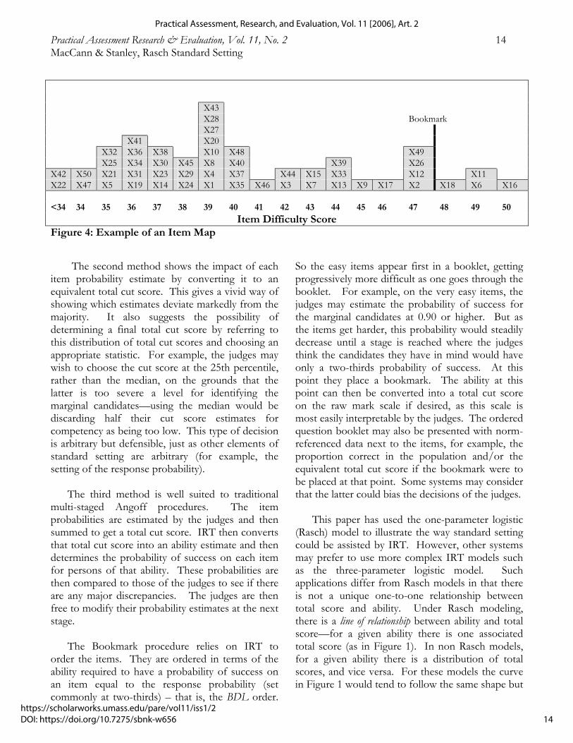
A variant of the bookmarking procedure is

called item mapping, in which a histogram visual display is used to present the data in a more compact format. As presented by Wang (2003), this technique uses the one parameter (Rasch) model, using the item difficulties to order the items, with a response probability of 0.5. This use of the Rasch model with an RP of 0.5 simplifies matters conceptually as it removes any need for the concept of the BDL. In this case the BDLs are equal to the item difficulties (see Equation 4), so the whole process can be explained to the judges in terms of the item difficulties. This procedure uses the item difficulty data from Table 4, but instead of presenting it as a table, it is presented as a histogram. A linear transformation is applied to the item difficulties to transform them into an arbitrary scale, but one that seems more meaningful to the judges than the logit scale. At the same time this transformation is used to coarsen the

10



Practical Assessment Research & Evaluation, Vol. 11, No. 2 11 MacCann & Stanley, Rasch Standard Setting scale by clumping some adjacent item difficulties into the one value, so that the histogram fits onto a single page. For example, the item difficulties presented in Table 4 were first multiplied by 4, and then 40 was added to this product. The resulting transformed difficulties were then rounded to the nearest integer. They are then plotted as a histogram as shown in Figure 4, with the height of the columns being the number of test items on the rounded difficulty value, and with the item ID numbers being shown in each column.

The judges are able to scan the columns of the histogram, noting the items in each column, and determine the column where the marginal band candidates are considered to have a 50:50 chance of being correct on such items (RP=0.5). Once a judge has tentatively placed a bookmark, this sets an ability level. Given this ability level, the probability of success of the marginal band candidates on nearby items can be found from Equation 1 and given to the judge as additional information to help confirm the judgement.

This procedure requires that the judges be

familiar with the items, so that a booklet that sorted the items in IRT difficulty order, as in Figure 3, would still seem a desirable requirement. With items of similar difficulty printed next to each other in the booklet, the judges would not have to turn pages of the test to locate items that appear together in the one histogram column.

Can the item mapping procedure be used with

response probabilities other than 0.5? It can, but the explanation of the process to the judges is more complicated with BDLs being used instead of item difficulties. Instead of linearly transforming the item difficulties, it is the BDLs that are transformed. For example in Table 4, a BDL column corresponding to a response probability of two-thirds is given, immediately to the right of the item difficulties column. These BDL values can be linearly transformed and presented as a histogram similar to that in Figure 4. The judges then attempt to find the column where the probability of success on the items in the column is two-thirds for the marginal band candidates.

CONCLUSIONS This paper has indicated four ways in which

IRT could be used to improve standard setting. The first three methods are consistent with an Angoff multi-staged approach while the last method and a variant use the bookmarking technique. In each case, some useful norm-referenced data has been added to the IRT data. Whether or not this additional data is acceptable in some educational systems may depend on the extent to which standards are emphasised independently of performance. Such educational systems may wish to suppress this norm-referenced data, or to introduce it at a different stage. For these methods to be of use, it is important that a representative sample of student data is available at the time when judging is taking place. In systems where time pressure in reporting results is an issue, these procedures may not be practicable.

The first method is used to provide data before

the judges make (or endorse) Angoff item probability estimates. Before a single judgement has been made, the judges are supplied with a table showing all the total scores and, for each score, the probability of success on every item for the candidates gaining that score. In this technique, the judges are forming a mental image of the marginal candidates and are focusing on rows of data, which seem to reflect the item probability estimates that such a group would be expected to obtain. This has several appealing features. It is probably quicker than the normal item by item Angoff ratings. It demonstrates the differences in item difficulty (as shown by the differences in probability of success) at different points of the scale. It provides IRT probabilities of success based on a clearly stated model, rather than judges estimates, which can be quite fallible. For evidence of the possible inaccuracy of such estimates see Bejar, 1983; Mills and Mellican, 1988; Shepard, 1995; Goodwin, 1999. At the same time, if the educational system is such that it prefers to leave the final decision on the probability estimates to the judges, the data provided may be used to inform the judges’ decisions rather that dictate it. The judges would then use the data as a guide in submitting their own probability estimates.

11




Q9 Proportion correct = 0.32 Estimated cut score = 40.4

Evaluate 2

212 ⎟⎠⎞

⎜⎝⎛ .

………………………………………………………………………………………………………..

JUDGES SET BOOKMARK HERE

Q17 Proportion correct = 0.26 Estimated cut score = 42.8 Susan is paid an allowance of 25 cents per kilometre (km) to drive to and from work. She lives 17 km from work and works 4 days a week. Calculate her allowance for one week. ………………………………………………………………………………………………………..

Q26 Proportion correct = 0.25 Estimated cut score = 43.1

131222 =+X . Find the value of X. ………………………………………………………………………………………………………

Q12 Proportion correct = 0.25 Estimated cut score = 43.5 Peter’s grandmother was 42 years old when Peter was born. His grandmother was three times his age when she retired. How old was Peter when his grandmother retired? ……………………………………………………………………………………………………….

Figure 3 :Example layout of items arranged in order of ability at which P=0.667 and the selection of a bookmark

12




Table 4: A subset of the items arranged in BDL order (RP=0.667) and showing estimated Total Cut Scores

Item Proportion correct

IRT item difficulty

BDL value (RP = 0.667)

Corresponding Total Cut Score

30 0.70 -0.861 -0.168 23.8 23 0.70 -0.857 -0.164 23.8 38 0.68 -0.767 -0.074 24.7 14 0.67 -0.687 0.006 25.5 29 0.65 -0.537 0.156 26.9 45 0.63 -0.494 0.199 27.3 24 0.63 -0.468 0.225 27.5 8 0.61 -0.349 0.344 28.7

27 0.60 -0.338 0.355 28.8 10 0.60 -0.327 0.366 28.9 20 0.60 -0.324 0.369 28.9 1 0.59 -0.288 0.405 29.2

43 0.58 -0.244 0.449 29.6 28 0.57 -0.178 0.515 30.2 4 0.57 -0.136 0.557 30.6

35 0.56 -0.114 0.579 30.8 48 0.55 -0.064 0.629 31.2 37 0.54 0.008 0.701 31.9 40 0.53 0.043 0.736 32.2 46 0.47 0.323 1.016 34.5 44 0.46 0.384 1.077 35.0 3 0.43 0.582 1.275 36.6 7 0.40 0.758 1.451 37.9

15 0.39 0.772 1.465 38.0 39 0.36 0.897 1.590 38.8 13 0.34 1.007 1.700 39.6 33 0.34 1.029 1.722 39.7 9 0.32 1.141 1.834 40.4

17 0.26 1.561 2.254 42.8 26 0.25 1.630 2.323 43.1 12 0.25 1.702 2.395 43.5 49 0.22 1.803 2.496 43.9 2 0.23 1.821 2.514 44.0

18 0.19 2.066 2.759 45.0 11 0.19 2.231 2.924 45.6 6 0.16 2.280 2.973 45.8

16 0.17 2.442 3.135 46.3

13




X43 X28 Bookmark X27 X41 X20 X32 X36 X38 X10 X48 X49 X25 X34 X30 X45 X8 X40 X39 X26 X42 X50 X21 X31 X23 X29 X4 X37 X44 X15 X33 X12 X11 X22 X47 X5 X19 X14 X24 X1 X35 X46 X3 X7 X13 X9 X17 X2 X18 X6 X16 <34 34 35 36 37 38 39 40 41 42 43 44 45 46 47 48 49 50

Item Difficulty Score

Figure 4: Example of an Item Map

The second method shows the impact of each item probability estimate by converting it to an equivalent total cut score. This gives a vivid way of showing which estimates deviate markedly from the majority. It also suggests the possibility of determining a final total cut score by referring to this distribution of total cut scores and choosing an appropriate statistic. For example, the judges may wish to choose the cut score at the 25th percentile, rather than the median, on the grounds that the latter is too severe a level for identifying the marginal candidates—using the median would be discarding half their cut score estimates for competency as being too low. This type of decision is arbitrary but defensible, just as other elements of standard setting are arbitrary (for example, the setting of the response probability).

The third method is well suited to traditional

multi-staged Angoff procedures. The item probabilities are estimated by the judges and then summed to get a total cut score. IRT then converts that total cut score into an ability estimate and then determines the probability of success on each item for persons of that ability. These probabilities are then compared to those of the judges to see if there are any major discrepancies. The judges are then free to modify their probability estimates at the next stage.

The Bookmark procedure relies on IRT to

order the items. They are ordered in terms of the ability required to have a probability of success on an item equal to the response probability (set commonly at two-thirds) – that is, the BDL order.

So the easy items appear first in a booklet, getting progressively more difficult as one goes through the booklet. For example, on the very easy items, the judges may estimate the probability of success for the marginal candidates at 0.90 or higher. But as the items get harder, this probability would steadily decrease until a stage is reached where the judges think the candidates they have in mind would have only a two-thirds probability of success. At this point they place a bookmark. The ability at this point can then be converted into a total cut score on the raw mark scale if desired, as this scale is most easily interpretable by the judges. The ordered question booklet may also be presented with norm-referenced data next to the items, for example, the proportion correct in the population and/or the equivalent total cut score if the bookmark were to be placed at that point. Some systems may consider that the latter could bias the decisions of the judges.

This paper has used the one-parameter logistic

(Rasch) model to illustrate the way standard setting could be assisted by IRT. However, other systems may prefer to use more complex IRT models such as the three-parameter logistic model. Such applications differ from Rasch models in that there is not a unique one-to-one relationship between total score and ability. Under Rasch modeling, there is a line of relationship between ability and total score—for a given ability there is one associated total score (as in Figure 1). In non Rasch models, for a given ability there is a distribution of total scores, and vice versa. For these models the curve in Figure 1 would tend to follow the same shape but

14



Practical Assessment Research & Evaluation, Vol. 11, No. 2 15 MacCann & Stanley, Rasch Standard Setting would resemble a scatterplot, with multiple abilities for each total score.

In such cases, the total score scale can be often

replaced by the ability scale for the methods presented in this paper. For example, the probability data in Table 1 could be generated using a non Rasch model, but the far left column would be replaced by an ability scale. The judges could still encircle the appropriate probability estimates and find the row that best expressed the desired standard of achievement. This would then define a standard in terms of the ability scale. If desired, this scale could be linearly transformed to a scale more closely resembling the raw mark scale. Similarly for the Table 2 method, the corresponding total cut score could be removed and replaced by a linearly transformed ability scale.

The procedure based on the Table 3 data,

however, is incompatible with non Rasch models. After summing the Angoff ratings, a total cut score on the raw mark scale is obtained. There is no one-to-one relationship between this cut score and ability—this cut score could be associated with many ability scores, depending on the particular items on which a student was correct. Having said this, a conversion between the raw mark scale and the ability scale can always be obtained through approximate methods (e.g. equating percentiles in the ability and raw score distributions). As the judges generally understand and prefer a raw mark scale, some systems may wish to convert to the raw mark scale, even though it is against the spirit of non Rasch models.

A second issue concerns Angoff standard

setting with constructed response items. There are Rasch models that accommodate constructed response items (for example, Andrich’s extended logistic model in the RUMM software package; Master’s (1982) partial credit model). These models give a one-to-one relationship between total score and ability, as shown in Figure 1. On a constructed response item the Angoff judges estimate a cut score as a mark, rather than as a probability. Despite this difference, useful IRT data can be provided to the judges from such packages. For example, a table similar to Table 1 can be constructed with the total mark and percentile

columns, but with the probabilities for each item replaced by expected scores (which are obtained from the software). Suppose for example that Item 1 had a maximum possible score of 10. Then the table might show that students gaining a total score on the test of 85 (/100) had an expected score of 7.8 (/10) on Item 1. The judges could encircle the expected score for Item 1 that is closest to their cut score, and then repeat the process for Item 2 etc until they were confident of selecting the appropriate row that best reflected the pattern of encircled cut scores. This row then gives the total cut score.

The bookmarking method may also be

performed with constructed response items, with Rasch or non Rasch models. Whereas multiple choice or dichotomously scored items appear only once in the ordered test booklet, constructed response items appear several times depending on the number of score points available. Associated with each score point is a BDL—such an item with score points of 0, 1, 2, 3 would appear three times in the booklet, once for each non zero score point. The BDL for 1 would appear first in the booklet, the BDL for 2 would appear at a more difficult location, and the BDL for 3 would appear at the most difficult location of the three points. Suppose the response probability is two-thirds. Then the BDL for a score point in a polychotomous item is the ability level required to have a two-thirds probability of gaining that score or above.

The Bookmark procedure has an advantage

over the Angoff method in that it avoids the item by item judgements that can be tedious and difficult for the judges. However there are some technical issues to consider in this procedure, relating to the choice of the response probability and the choice of IRT model. As the Bookmark procedure involves an ordering of the items, Beretvas (2004) has shown how the choice of IRT model and response probability may affect the rank order in which the items would be presented (the BDL). In Beretvas’ data set, Spearman correlations between bookmark difficulty locations were computed for various combinations of IRT model and response probability. These were generally above 0.90 but did not give perfect agreement. Given that there is often considerable variation in where judges set

15



Practical Assessment Research & Evaluation, Vol. 11, No. 2 16 MacCann & Stanley, Rasch Standard Setting their bookmarks, with the final cut score being the average of the logit values, it is likely that the effect of slightly differing rank orders of the items would not have a great effect on the cut score. However, this would be a useful area for future research.

REFERENCES

Andersen, E.B. (1973). A goodness of fit test for the

Rasch model. Psychometrika, 38, 123-140. Andrich, D., Sheridan, B., Lyne, A. and Luo, G. (2000).

RUMM: a Windows-based item analysis employing Rasch unidimensional measurement models. Perth: Murdoch University.

Angoff, W.H. (1971). Scales, norms and equivalent

scores. In R.L. Thorndike (Ed.), Educational Measurement. (2nd ed.). Washington, D.C.: American Council on Education.

Bejar, I. (1983). Subject matter experts’ assessment of

item statistics. Applied Psychological Measurement, 7, 303-310.

Beretvas, S.N. (2004). Comparison of bookmark

difficulty locations under different item response models. Applied Psychological Measurement, 28, 25-47.

Berk, R. (1996). Standard setting: the next generation.

Applied Measurement in Education, 9, 215-235. Board of Studies NSW (2003). The standards-setting

operation: handbook for judges. Board of Studies NSW, Sydney.

Buckendahl, C.W., Smith, R.W., Impara, J.C. and Plake,

B.S. (2002). A comparison of Angoff and bookmark standard setting methods. Journal of Educational Measurement, 39, 253-263.

Cross, L.H., Impara, J.C., Frary, R.B. and Jaeger, R.M.

(1984). A comparison of three methods for establishing minimum standards on the National Teacher Examinations. Journal of Educational Measurement, 21, 113-130.

Embretson, S.E. and Reise, S.P. (2000). Item response theory

for psychologists. Mahwah, NJ: Lawrence Erlbaum Associates, Publishers.

Goodwin, L.D. (1999). Relations between observed

item difficulty levels and Angoff minimum passing

levels for a group of borderline candidates. Applied Measurement in Education, 12, 13-28.

Hambleton, R.K., Swaminathan, H. and Rogers, H.J.

(1991). Fundamentals of item response theory. Newbury Park: Sage.

Jaeger, R. (1982). An Iterative Structured Judgment

Process for Establishing Standards on Competency Tests of Theory and Application. Educational Evaluation and Policy Analysis, 4, 461-475.

Kane, M.T. (1987). On the use of IRT models with

judgmental standard setting procedures. Journal of Educational Measurement, 24, 333-345.

Lord, F.M. (1952). A theory of test scores. Psychometric

Monograph, No. 7. Lord, F.M. (1953). The relation of test scores to the trait

underlying the test. Educational and Psychological Measurement, 13, 517-548.

Lord, F.M. (1980). Applications of item response theory to

practical testing problems. Hillsdale, NJ: Lawrence Erlbaum Associates.

Linn, R. (1978). Demands, cautions and suggestions for

setting standards. Journal of Educational Measurement, 15, 301-308.

MacCann, R.G. and Stanley, G. (2004). Estimating the

standard error of the judging in a modified-Angoff standards setting procedure. Practical Assessment Research & Evaluation. http://pareonline.net/

Masters, G.N. (1982). A Rasch model for partial credit

scoring. Psychometrika, 47, 149-174. Mills, C.N. and Melican, G.J. (1988). Estimating and

adjusting cutoff scores: Future of selected methods. Applied Measurement in Education, 1, 261-275.

Mitzel, H.C., Lewis, D.M., Patz, R.J. and Green, D.R.

(2001). The bookmark procedure: psychological perspectives. In G. J. Cizek (Ed.), Setting performance standards (pp. 249-281). Mahwah, NJ: Lawrence Erlbaum.

Morrison, H., Busch, J. and D'Arcy, J. (1994). Setting

reliable national curriculum standards: a guide to the Angoff procedure. Assessment in Education, 1, 181-199.

16



Practical Assessment Research & Evaluation, Vol. 11, No. 2 17 MacCann & Stanley, Rasch Standard Setting Norcini, J., Lipner, R., Langdon, L. and Strecker, C.

(1987). A comparison of three variations on a standard-setting method. Journal of Educational Measurement, 24, 56-64.

Norcini, J., Shea, J. and Kanya, D. (1988). The effect of

various factors on standard setting. Journal of Educational Measurement, 25, 57-65.

Popham, W. (1978). As always provocative. Journal of

Educational Measurement, 15, 297-300. Rasch, G. (1960/1980). Probabilistic models for intelligence

and attainment tests. University of Chicago Press, Chicago, Illinois.

Rasch, G. (1966). An item analysis which takes

individual differences into account. British Journal of Mathematical and Statistical Psychology, 19, 49-57.

Reckase, M.D. (2000). Survey and evaluation of recently

developed procedures for setting standards on educational tests. In Student performance standards on the National Assessment of Educational Progress: Affirmation and improvements. Washington, DC: National Assessment Governing Board.

Reid, J. (1991). Training judges to generate standard-setting data. Educational Measurement: Issues and Practice, 10, 11-14.

Shepard, L.A. (1995). Implications for standard setting

of the National Academy of Education evaluation of the National Assessment of Educational Progress achievement levels. Proceedings of Joint Conference on Standard Setting for Large-scale Assessments, pp 143-160. Washington, D.C.: NAGB and the NCES.

van der Linden, W.J. (1982). A latent trait method for

determining intrajudge consistency in the Angoff and Nedelsky techniques of standard setting. Journal of Educational Measurement, 4, 295-308.

van der Linden, W.J. and Hambleton, R.K. (Eds.)

(1997). Handbook of modern item response theory. New York: Springer.

Wang, N. (2003). Use of the Rasch IRT model in

standard setting: an item-mapping method. Journal of Educational Measurement, 40, 231-253.

Wiliam, D., (1996). Meanings and consequences in

standard setting. Assessment in Education, 3, 287-307.

Citation

MacCann, Robert G. & Gordon Stanley (2006). The use of Rasch modeling to improve standard setting. Practical Assessment Research & Evaluation, 11(2). Available online: http://pareonline.net/getvn.asp?v=11&n=2

Authors Dr Robert MacCann is Head, Measurement and Research Services, within the NSW Board of Studies, Sydney Australia. Dr Gordon Stanley is President of the NSW Board of Studies, Adjunct Professor, School of Policy and Practice, in the Faculty of Education and Social Work, University of Sydney and Emeritus Professor of Psychology, University of Melbourne.

Contact

Dr Robert MacCann, Head, Measurement & Research Services, Board of Studies NSW GPO Box 5300, Sydney 2001 Australia [email protected]

Descriptors

Standard setting; modified Angoff procedures; item response theory; Rasch modeling, judging feedback.

17



http://pareonline.net/getvn.asp?v=11&n=2

The Use of Rasch Modeling To Improve Standard Setting

Documents

Transcript of The Use of Rasch Modeling To Improve Standard Setting