The U.S. Dollar Safety Premium

The U.S. Dollar Safety Premium

Matteo Maggiori∗

Current draft: March 2013

Abstract

I show that the US dollar earns a safety premium versus a basket of foreign currencies

and that this premium is particularly high in times of global financial stress. These

findings support the view that the dollar acts as the reserve currency for the

international monetary system and that it is a natural safe haven in times of crisis,

when a global flight to quality toward the reserve currency takes place. During such

episodes, investors are willing to earn negative expected returns as compensation

for holding safe dollars. I estimate the time varying dollar safety premium by using

instrumental variable techniques to condition information down.

JEL classification: F31, G12, G15.

Keywords: Exchange Rates, Reserve Currency, Exorbitant Privilege, Cur-

rency Returns, Time-varying Risk.

∗New York University, Stern School of Business, NBER, and CEPR. [email protected] would like to thank the members of my PhD committee for advice well beyond their duties: NicolaeGarleanu, Pierre-Olivier Gourinchas, Martin Lettau, Maurice Obstfeld, and Andrew Rose. I would alsolike to thank: Richard Clarida, Nicolas Coeurdacier, Yesol Huh, Ralph Koijen, Hayne Leland, HannoLustig, Anna Pavlova, Helene Rey, Andreas Stathopoulos, Jerry Tsai, Adrien Verdelhan, and seminarparticipants at the AFA meeting, UNC Junior Faculty Roundtable, Joint Berkeley-Stanford PhD Seminar,LBS PhD Transatlantic Conference, UC Berkeley, NYU Volatility Institute Conference. I gratefullyacknowledge the financial support of the White Foundation and the UC Berkeley Institute for Businessand Economics Research.

The international monetary system has long been characterized by the existence of a

reserve currency: first it was gold, then the British pound sterling, and most recently the

United States dollar. Conventional wisdom is that the reserve currency plays a special

role in the international monetary system by acting as a safe asset during periods of rare,

but intense, crisis. During such episodes a global flight to quality takes place: investors

look for safe assets in international financial markets, concentrating their demand on

short-term liabilities denominated in the reserve currency. The reserve currency should

therefore, on average, earn a safety premium: the compensation that investors require

to short this currency and invest in a basket of foreign currencies. This premium should

vary over time and, in particular, be highest in times of global financial stress.

I document that this is exactly the role played by the US dollar during the modern

floating exchange rate period (1973-2010). Figures 12-13 plot my estimates of the dollar

safety premium. Periods of crisis are highlighted. The dollar safety premium is on average

1% on an annual basis. It increased to as much as 52% following the collapse of Lehman

Brothers in October 2008.

The recent global financial crisis has been a painful reminder of the economic logic

behind my results. The preceding period had been characterized by buoyant financial

markets, low risk premia and an expanding world economy. The dollar had been on

a depreciating trend since 2002 and the US was a large external debtor. During the

crisis, and especially at the time of the Lehman Brothers default, the dollar experienced

a knee-jerk appreciation. At the time, market commentary emphasized the global search

for safe assets, which culminated in extraordinary demand for short-term US liabilities.

Surprisingly this happened despite the US being a substantial international debtor with

a worsening fiscal position and the US economy being among the worst hit by the global

crisis. After June 2009, as the most acute phase of the crisis faded and markets began

to stabilize, the dollar started to depreciate. In the words of the US Secretary of the

Treasury, Timothy F. Geithner:1

“Over the last two and a half years, you have seen a period when the world

was most concerned about the potential risk of global depression, was most

concerned about the possibility of systemic collapse; you saw the world seek

the safety of the risk-free asset of the United States. The dollar generally

rose over that period of time, and as the world has become progressively more

confident some of those safe-haven flows have been reversed.”

These facts can be interpreted in terms of the dollar safety premium. When a shock,

1CNBC interview on November 11, 2010.

1

such as the Lehman Brothers collapse, hits the economy, the dollar safety premium

increases on impact as investors demand more dollars. This causes a dollar appreciation

on impact to the point of overshooting:2 to generate a high safety premium the dollar

appreciates to such an extent that it is expected to depreciate in the future. The expected

negative return from holding dollars is the compensation for its safety. As the shock

fades, investor demand for the dollar decreases, thus triggering a dollar depreciation and

a reduction in the dollar safety premium.

To estimate the dollar safety premium I first formalize the exchange rate dynamics

in terms of risk premia (Section I). The theory section of this paper is intentionally

minimalist so that the identification in the data is not strictly model dependent and

its implications encompass a larger set of theoretical structural models. To estimate

the dollar returns I employ a novel dataset of currency returns and a new measure of

financially weighted exchange rates. I estimate the time varying dollar safety premium by

employing techniques on information conditioning and instrumental variables developed

in the empirical asset pricing literature (Campbell (1987), Harvey (1989), Duffee (2005)).

Despite conventional wisdom on the role of the reserve currency during crises being

widely discussed in the financial press3 and the clear importance of the subject for the

global economy, relatively little academic literature has been devoted to the topic. The

importance of the reserve currency during times of crisis was first noted by Bagehot (1873)

in his treatise on London money markets. Triffin (1960) emphasized the possibility that

the key country, which runs large deficits in its aim to supply currency to the rest of the

world, could fall victim to a run on its currency in times of global stress.

In the context of more recent studies, this paper contributes to the literature on the

role of the dollar in the international monetary system. This literature has investigated

whether dollar denominated assets offer lower returns than comparable foreign currency

assets, and whether this return differential is predictable. Gourinchas and Rey (2007a,b)

find a positive and predictable return differential and call it the US “exorbitant privilege”.

Curcuru, Dvorak, and Warnock (2008, 2009), and Lane and Milesi-Ferretti (2009) show

that systematic bias in revisions to the US balance of payments data leads to an

overestimation of the return differential. More recently, Forbes (2010), Habib (2010)

and revised estimates from Gourinchas and Rey (Gourinchas, Govillot, and Rey (2010))

find a positive return differential.

2This effect is reminiscent of the famous Dornbusch overshooting (Dornbusch (1976)). However, theeffect here is caused by changes in the risk premium that are absent from the Dornbusch model. Riskpremium effects to the level of the exchange rate were introduced by Obstfeld and Rogoff (1998).3For a recent example from the Financial Times: “traders have long been using the US dollar as a proxy

for risk appetite: its decline a signal that markets were relaxed about global economic growth, and itsrise a gauge of haven flows as sentiment deteriorated” (article by Jamie Chisholm on October 11, 2010).

2

The main difficulty in accurately estimating returns for long time spans is the coarse

detail that national statistics provide on the nature of assets held across borders. Even

within asset categories such as equity, foreign direct investment (FDI), and bonds, there

exists substantial cross-sectional heterogeneity that could swamp any international asset

return differential.

By focusing on the US currency return (i.e. the return differential between US and

rest of the world (RoW) risk-free bonds). With a simple theoretical decomposition, I

show that this return is a direct component of the return differential of any other asset

class (equities, FDI, corporate bonds). The advantage of focusing on the currency return

is that I can use assets that are comparable across countries and for which returns are

accurately measured. Clearly this return differential does not strictly imply a return

differential for the US external position; that will depend on the exact composition of the

assets held in the US external account. However, should there be a return differential

between comparable US and RoW assets, then it should exist irrespective of whether the

assets are actually held in the US external account or not.

I estimate the conditional dollar safety premium instead of focusing on unconditional

returns, as is done in the literature discussed above. In fact, I show that the unconditional

dollar safety premium, while positive, is not statistically significant. This is not surprising

given the low mean returns and the volatility of exchange rates. Nor is it uncommon: it is

a feature shared by many other risk premia in finance, including the equity risk premium.

However, the hypothesis that the dollar acts as a key currency for the global financial

system has the conditional implication that its safety premium should increase during

times of global financial stress. Testing this conditional statement, I provide significant

statistical evidence in favor of a positive dollar safety premium, particularly in times of

crisis.

Authors have advanced a variety of possible explanations for the return differential:

the superior ability of the US to time its investments compared to the RoW (Curcuru et al.

(2009)), US exorbitant privileges (Gourinchas and Rey (2007a)), and the superior financial

development of the US (Caballero, Farhi, and Gourinchas (2008), Mendoza, Quadrini, and

Rıos Rull (2009), Forbes (2010), Maggiori (2011)). In this paper I suggest a simple risk

based rationalization of the return differential. A portfolio that is short dollars and long

a basket of foreign currencies earns an average positive return to compensate for the risk

of negative returns in times of crisis, when the dollar appreciates due to the global flight

to quality toward the reserve currency. Such a portfolio is risky, because it has a negative

payoff in the bad states of the world. Time variation in this risk premium generates

predictable movements in dollar returns.

3

This paper is also related to the literature on the failure of the Uncovered Interest

Parity (UIP) condition and the carry trade. Fama (1984) documents systematic deviations

from the UIP condition, stating that the exchange rate movement should offset the interest

rate differential, so that returns from currency speculation are zero. Among a vast

empirical literature, important recent contributions are Lustig and Verdelhan (2007),4

Burnside, Eichenbaum, Kleshchelski, and Rebelo (2011) and Lustig et al. (2010, 2011),

who estimate asset pricing models of currency returns with systematic deviations from

UIP. The dollar safety premium estimated in this paper is also a deviation from UIP. The

focus of this paper, however, is different from the UIP or carry trade literature: I am

interested in the time series properties of the dollar safety premium, while this literature

is mainly focused on the cross section of currency returns. I estimate a conditional asset

pricing model, while the papers above focus on unconditional moments.5 Within the UIP

literature the most closely related papers are Cumby (1988), who estimates conditional

covariances of bilateral currency returns with US consumption, and Lustig, Roussanov,

and Verdhelan (2010), who estimate a countercyclical dollar risk premium using the

average forward rate on a basket of foreign currencies and US industrial production

growth.

I Theory

Consider a two country world: US and RoW. By simple no-arbitrage asset pricing,

there exist two stochastic discount factors (SDF), one for each country, such that

1 = Et[Λt+1Rt+1]; 1 = Et[Λ∗t+1R

∗t+1],

where Λt+1 is the US SDF, and Rt+1 is any US asset return. RoW variables are denoted

by ∗. The exchange rate is defined as the US price of RoW currency and denoted Et (a

decrease in the exchange rate is a US dollar appreciation).

Proposition 1. Assume no arbitrage and that all assets are traded internationally, then

there exist two SDFs such that

Λt+1 = Λ∗t+1

EtEt+1

. (1)

A simple proof is relegated to Appendix A. The economic logic behind the proposition

is provided by Backus, Foresi, and Telmer (2001) and Brandt, Cochrane, and Santa-Clara

4See also Burnside (2011) and Lustig and Verdelhan (2011).5Papers on the cross sections of currency returns most commonly sort currencies into portfolios based on

the level of their interest rates. This sorting is close to a model where the only conditioning informationis the interest rate.

4

(2006). US and RoW agents agree on the prices of all assets that they can trade. Under

complete markets, the span of assets covers the entire state space so that agents agree on

all possible prices. Under this condition, the SDF of each country is unique and obeys

the relationship in equation (1). However, if markets are not complete agents need only

agree on the prices of assets that can actually be traded. For each country there exists an

infinite set of valid SDFs. Equation (1) does not need to hold between any two arbitrary

SDFs. However, the equation can be considered a definition for SDFs in one country

given a choice of SDF in the other country. For simplicity I assume here that markets are

complete.

In this setting it is possible to derive an intuitive decomposition of the expected excess

return of investing in a RoW asset by shorting a US asset.

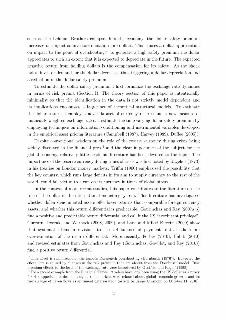
Proposition 2. Assume that asset returns, SDFs and the exchange rate are jointly log-

normally distributed. Then the expected excess return in dollars of the RoW asset over

the US asset is

Et[r∗t+1 + ∆et+1 − rt+1] +

1

2V art(r

∗t+1 + ∆et+1)−

1

2V art(rt+1) = (2)

−Covt(m∗t+1, r∗t+1) + Covt(mt+1, rt+1)︸︷︷︸

domestic risk

+Covt(r∗t+1,∆et+1)− Covt(mt+1,∆et+1)︸︷︷︸

exchange rate risk

.

The simple derivation is in Appendix A. Lower cases denote natural logarithms. The

LHS is the expected excess log return plus Jensen’s inequality terms due to the use

of logarithms. The RHS shows that the risk premium can be decomposed into four

components:

• −Covt(m∗t+1, r∗t+1): RoW asset risk premium over the RoW risk-free rate, expressed

in RoW currency;

• −Covt(mt+1, rt+1): US asset risk premium over the US risk-free rate, expressed in

dollars;

• Covt(r∗t+1,∆et+1): RoW asset is riskier for US investors if it pays higher when the

dollar depreciates; and

• −Covt(mt+1,∆et+1): dollar currency safety premium.

Intuitively consider the case of RoW and US equities. A US investor who buys RoW

equities by selling US equities will earn the RoW equity premium, pay the US equity

premium, and earn/pay a compensation for foreign exchange risk.

5

The first two terms on the RHS of equation (2) are typical of closed economy analysis.

Flight to quality, in that setting, is manifested as the increase in the risk premium of

riskier assets (say, equities) in times of economic stress. The last two terms add the

international dimension to the analysis of flight to quality: the exchange rate. In this

light, global flight to quality toward the dollar is manifested as an increase in the risk

premium of investing in RoW currency by funding in dollars in times of economic stress.

The last term on the RHS of equation (2) is identified to be the dollar safety premium

($SPt) by observing that in the case of the US and RoW risk-free rate, equation (2)

reduces to

$SPt ≡ r∗f,t+1 + Et[∆et+1]− rf,t+1 +1

2V art(∆et+1) = −Covt(mt+1,∆et+1). (3)

The dollar safety premium is positive if the dollar appreciates when the SDF increases.

Logically, the dollar is safe if it appreciates in times of economic stress. Those times

are characterized by high marginal utility growth, and therefore a high SDF. The safety

premium is closely related to the deviation from uncovered interest parity (UIP). The UIP

condition can be stated in logs as Et[r∗f,t+1 + ∆et+1 − rf,t+1] = 0 . Therefore, up to the

Jensen’s inequality term 12V art(∆et+1) the currency risk premium is the deviation from

UIP.

The last step to make the above equations operational is to specify the functional

form of the SDFs in equation (1). Mt+1 = At − BtRwt+1 (A > 0, B > 0) is the unique

US SDF lying in the payoff space: it consists of a long position in the US risk-free rate

(At/Rf,t+1) and a short position in the world equity portfolio expressed in dollars (Bt). If

one identifies the world equity portfolio to be the market portfolio, the above SDF yields

the CAPM. By substituting the log approximation mt+1 = at− btrwt+1 to Mt+1 in equation

(3), the dollar safety premium reduces to

$SPt = −Covt(mt+1,∆et+1) = btCovt(rwt+1,∆et+1). (4)

There are two possible sources of time variation of the risk premium: time varying price of

risk (bt), and time varying quantity of risk (covariance). Furthermore, the two variations

could amplify each other (synchronous) or smooth each other (asynchronous). The

challenge is that the conditional covariance is not observable and needs to be estimated.

6

II Data

I build indices for the dollar currency return versus a basket of foreign currencies

(the RoW currency), as well as comparable indices for stock market returns at monthly

frequency for the period from January 1970 to March 2010.

I use the Morgan Stanley Capital International (MSCI) Barra indices to measure

stock market returns. These indices are weighted by the equity market capitalization of

each component country. The MSCI-Barra indices are widely used both in the financial

industry and in academia (Fama and French (1998)) to measure international stock

returns. They are particularly suited to this paper because they only include stocks

that can actually be traded by foreigners and are adjusted to make returns comparable

across countries’ different accounting and legal systems. I use a World index that includes

23 developed and 22 emerging countries, and a Developed index that only includes the

developed countries.6 The two indices are identical for the period 1970-1987 as the

emerging countries are assigned a zero weight, and progressively differ for the period

1988-2010 as the emerging countries’ market capitalization increases. Figure 1 plots the

two total return7 equity indices.

For both the Developed and World indices I build US dollar spot exchange rate indices,

shown in Figure 2. These are market capitalization8 weighted exchange rate indices. For

example, the dollar exchange rate corresponding to the World index measures the value

of the dollar versus a basket of currencies, where the weight of each bilateral exchange

rate9 corresponds to the weight of the country in the equity World index excluding the

United States.

Financially weighted exchange rates are a notable improvement over the trade

weighted or equally weighted exchange rates more commonly used in the literature to

analyze broad movements in currency values. Lane and Shambaugh (2010) show that

trade weighted indices are insufficient to understand the financial impact of currency

movements and argue for financial exchange rates. They build financial exchange rates

6The “Developed index” corresponds to the MSCI Barra World index. The “World index” is built byusing the MSCI Barra World index for the period 1970-1987 and the MSCI Barra All Country Worldindex for the period 1988-2010. All indices are available on the MSCI Barra website and from Datastream.7These indices include dividend payouts.8The capitalization here refers to the equity market, which is particularly suited to this papers as it

makes equity and currency returns comparable. In general, it would be desirable to have a foreignexchange market capitalization weighted exchange rate, where the weight of each currency correspondsto its share of transactions in the foreign exchange market. Unfortunately, the foreign exchange marketis over-the-counter and, therefore, the necessary data is not readily available.9The data for bilateral spot exchange rates is from MSCI-Barra and is available from Datastream.

MSCI-Barra collects the data from Reuters’ multi contributors pages and WM-Reuters exchange rateservice.

7

for each country based on the currency composition of its foreign assets and liabilities.

Their exchange rates, although similar in spirit, differ from those employed here. To the

best of my knowledge, I am the first to use market capitalization based exchange rates.

To measure the dollar currency returns I first build estimates of the bilateral interest

rate differential between each country in the sample and the US, then weight each of these

differentials using the same MSCI-Barra weights as above. One would hope that such data

for the modern floating period 1973-2010 would be readily available and commonly shared

among papers in the literature. Surprisingly this is not the case. I detail the methods used

to build bilateral interest rate differentials in a separate note, “Note on New Estimates

of Currency Returns”. The resulting dataset is more extensive both in terms of the

currencies (53) and the time span (1970-2010) covered. Figure 3 shows the time series of

the interest rate differential indices for the World and the Developed indices.

The use of World and Developed countries weighted indices for both equity and

currency returns minimizes concerns about sovereign credit risk and investors’ access to

these assets for trading purposes. In particular, Emerging Markets have relatively little

weight in the World index until recent years, and all the results in this paper are robust

to focusing only on the more financially developed countries included in the Developed

index.

III Empirical Identification

To estimate the dollar safety premium in equation (4), I employ the instrumental

variable approach pioneered by Campbell (1987) and Harvey (1989). I follow most closely

the approach in Duffee (2005), who estimates the conditional covariance between US

consumption and US stock returns.

To lighten the notation I suppress the superscript w from the equity returns. The

covariance in equation (4) can be expressed as

rt+1 = Et[rt+1] + ηrt+1; ∆et+1 = Et[∆et+1] + ηet+1; (5)

Covt(rt+1,∆et+1) = Et[ηrt+1η

et+1]. (6)

This leads to a three stage procedure. The zero stage regressions are classic predictive

regressions of the type run by Campbell and Shiller (1988), and Fama (1984):

rt+1 = αrYrt + εrt+1; (7)

∆et+1 = αeYet + εet+1. (8)

8

where (Y rt , Y

et ) are vectors of predictive variables, such as the dividend-price ratio and the

interest rate differential. These regressions are dubbed zero stage regressions to distinguish

them from the first and second stage regressions typical of the GMM-IV setup that follows.

The role of the zero stage is to extract the predictable element (the time t expectation)

in equation (5) from stock returns and exchange rate changes.

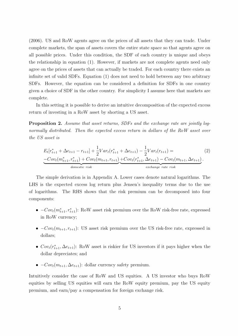
Denote the product of the residuals in equations (7-8) as Cov(rt+1,∆et+1) ≡ εrt+1εet+1.

The tilde is to stress that this is an ex-post estimate of the covariance and a time t + 1

object. The first stage regression projects this ex-post covariance on a set of instruments

Zt to obtain an estimate of the time t conditional covariance:

Cov(rt+1,∆et+1) = αzZt + ξt+1; (9)

Cov(rt+1,∆et+1) = αzZt. (10)

The choice of instruments is detailed in Section A . The conditional covariance (equation

(10)) is the estimate of the unobservable conditional covariance in equation (6).

The second stage regression estimates the model in equation (4) with instrumental

variables:

r∗f,t+1 + ∆et+1 − rf,t+1 +1

2V ar(∆et+1) = d0 + [d1 + d2bt]Cov(rt+1,∆et+1) + ωt+1, (11)

where V ar(∆et+1) ≡ (εet+1)2 is the ex-post estimate of the variance of the exchange rate,

and bt some observable proxy for the price of risk. This setup is quite flexible. For d2 = 0,

the only source of time variation in the dollar safety premium is the time variation of the

covariance. For d2 6= 0 a time varying price of risk also contributes to the time variation

of the dollar safety premium.

I estimate the first stage regression using OLS and allow for both heteroskedasticity

and serial correlation by using the Newey-West variance covariance matrix. To test the

hypothesis of time variation in the conditional covariance I use the asymptotically valid

χ2 test that all coefficients, except the constant, are jointly zero. However, I also report

the F test because of its prominent role in instrumental variable analysis.10 The zero

and second stage regressions are estimated jointly using GMM. This allows the second

stage standard errors to not only incorporate uncertainty deriving from the first stage

estimation (as it is standard in IV settings), but also the uncertainty deriving from the

zero stage estimation. The details of the GMM estimation are discussed in Appendix B.

10The χ2 and F test are asymptotically equivalent. In small samples the F test has wider confidenceintervals. However, in this paper the sample length and the number of restrictions are such that therejection regions are approximately identical for the two tests.

9

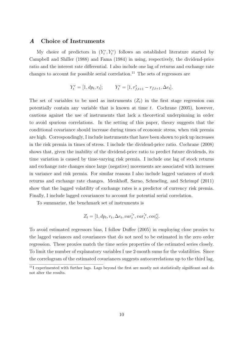
A Choice of Instruments

My choice of predictors in (Y rt , Y

et ) follows an established literature started by

Campbell and Shiller (1988) and Fama (1984) in using, respectively, the dividend-price

ratio and the interest rate differential. I also include one lag of returns and exchange rate

changes to account for possible serial correlation.11 The sets of regressors are

Y rt = [1, dpt, rt]; Y e

t = [1, r∗f,t+1 − rf,t+1,∆et].

The set of variables to be used as instruments (Zt) in the first stage regression can

potentially contain any variable that is known at time t. Cochrane (2005), however,

cautions against the use of instruments that lack a theoretical underpinning in order

to avoid spurious correlations. In the setting of this paper, theory suggests that the

conditional covariance should increase during times of economic stress, when risk premia

are high. Correspondingly, I include instruments that have been shown to pick up increases

in the risk premia in times of stress. I include the dividend-price ratio. Cochrane (2008)

shows that, given the inability of the dividend-price ratio to predict future dividends, its

time variation is caused by time-varying risk premia. I include one lag of stock returns

and exchange rate changes since large (negative) movements are associated with increases

in variance and risk premia. For similar reasons I also include lagged variances of stock

returns and exchange rate changes. Menkhoff, Sarno, Schmeling, and Schrimpf (2011)

show that the lagged volatility of exchange rates is a predictor of currency risk premia.

Finally, I include lagged covariances to account for potential serial correlation.

To summarize, the benchmark set of instruments is

Zt = [1, dpt, rt,∆et, var′rt , var

′et , cov

′t].

To avoid estimated regressors bias, I follow Duffee (2005) in employing close proxies to

the lagged variances and covariances that do not need to be estimated in the zero order

regression. These proxies match the time series properties of the estimated series closely.

To limit the number of explanatory variables I use 2-month sums for the volatilities. Since

the correlogram of the estimated covariances suggests autocorrelations up to the third lag,

11I experimented with further lags. Lags beyond the first are mostly not statistically significant and donot alter the results.

10

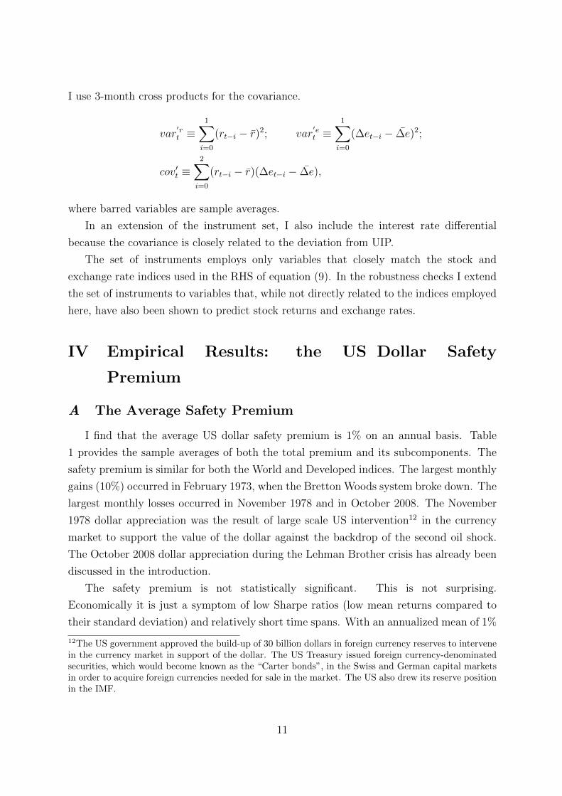
I use 3-month cross products for the covariance.

var′rt ≡

1∑i=0

(rt−i − r)2; var′et ≡

1∑i=0

(∆et−i − ∆e)2;

cov′t ≡2∑

i=0

(rt−i − r)(∆et−i − ∆e),

where barred variables are sample averages.

In an extension of the instrument set, I also include the interest rate differential

because the covariance is closely related to the deviation from UIP.

The set of instruments employs only variables that closely match the stock and

exchange rate indices used in the RHS of equation (9). In the robustness checks I extend

the set of instruments to variables that, while not directly related to the indices employed

here, have also been shown to predict stock returns and exchange rates.

IV Empirical Results: the US Dollar Safety

Premium

A The Average Safety Premium

I find that the average US dollar safety premium is 1% on an annual basis. Table

1 provides the sample averages of both the total premium and its subcomponents. The

safety premium is similar for both the World and Developed indices. The largest monthly

gains (10%) occurred in February 1973, when the Bretton Woods system broke down. The

largest monthly losses occurred in November 1978 and in October 2008. The November

1978 dollar appreciation was the result of large scale US intervention12 in the currency

market to support the value of the dollar against the backdrop of the second oil shock.

The October 2008 dollar appreciation during the Lehman Brother crisis has already been

discussed in the introduction.

The safety premium is not statistically significant. This is not surprising.

Economically it is just a symptom of low Sharpe ratios (low mean returns compared to

their standard deviation) and relatively short time spans. With an annualized mean of 1%

12The US government approved the build-up of 30 billion dollars in foreign currency reserves to intervenein the currency market in support of the dollar. The US Treasury issued foreign currency-denominatedsecurities, which would become known as the “Carter bonds”, in the Swiss and German capital marketsin order to acquire foreign currencies needed for sale in the market. The US also drew its reserve positionin the IMF.

11

and volatility of 8%, and using the standard formula σ/√T , it would take T ≥ 64 years to

detect statistical significance! This feature is shared by many risk premia in finance.13 For

example the US equity premium14 for the same period is also not statistically significant,

with a t-statistic of only 1.04.

Figures 4-5 show that the mean US dollar safety premium is fairly volatile across

different choices of samples, but remains positive throughout. Figure 4 plots the mean

safety premium for a rolling window with a fixed end in March 2010 (i.e. start-year to

March 2010). The highest safety premium (2% and above) is achieved when the sample

starts in the years 1983-1986.

A safety premium around 2% is comparable with the results in Lustig et al. (2010) and

Menkhoff et al. (2011), whose sample starts in 1983. Since these papers use an equally

weighted basket of currencies versus the dollar, in this section I also report results for

an equally weighted index. Figure 5 plots the mean safety premium for a reverse rolling

window with a fixed start in March 1970 (i.e. March 1970 to end-year). The recent crisis

decreases the mean premium by about 0.2%, but does not alter the overall results.

B Predictability of Currency and Equity Returns: Zero Stage

Regressions

While the dataset covers the period from 1970 to 2010, in the benchmark econometric

estimation I start the sample in January 1975 in order to eliminate possible concerns

about the inclusion of the pre-floating exchange rate period or the period immediately

following the break-down of the Bretton Woods system (December-March 1973).

Table 2 contains the results of the zero stage regressions. It re-establishes what are

by now classic results from previous studies using the new dataset. The regression in

equation (7) confirms not only the failure of the UIP condition, a coefficient different

from -1, but also the carry trade phenomenon, a positive coefficient. The deviation from

UIP is stronger for the Developed index than the World one, both in terms of point

estimate and statistical significance. This is due to the inclusion in the World index

of emerging market currencies, which have smaller deviations from UIP (Bansal and

Dahlquist (2000)).15 The regression in equation (8) confirms the predictability of stock

13It leads Cochrane (2005) to conclude that “this is a pervasive, simple, but surprisingly underappreciatedproblem in empirical asset pricing”.14Computed using the MSCI-Barra US equity Index and the 1-month US Libor rate.15A separate UIP regression that uses an emerging market exchange rate index, not reported here,confirms this result.

12

returns from the dividend-price ratio.16

Figures 6-7 plot the ex post estimate of the covariance Cov(rt+1,∆et+1) obtained as

the product of the residuals of zero order regressions.

C Time Varying Conditional Covariances: First Stage

Regressions

The first stage regression results in Table 3 show that the covariance is time varying

and predictable. The covariance predictability is robust to the choice of a subset of

instruments or to the addition of the interest rate differential, with the χ2 statistic rejected

at the 1% level in all cases. The most substantial drop in predictability occurs when the

lagged volatilities are excluded from the instrument set. The inclusion of the interest rate

differential in the set of instruments does not help to predict the covariance.

Furthermore, Panel B details that in a univariate regression where the interest rate

differential is the only instrument it has a negative coefficient. Theory actually predicts

a positive coefficient, as a high interest rate differential with the RoW should make the

dollar safer, thus increasing the covariance. In analogous univariate regressions for the

other instruments, I confirm that their relationship with the covariance has the sign

predicted by theory. While full results from univariate regressions are omitted in the

interest of space, the sign predictions and results are summarized in Table 4.

Kleibergen (2002) suggests that F statistics above 10 minimize concerns of weak

instruments. For this reason, while the χ2 test is the asymptotically efficient one, I

also report the F test. The F statistics of the first stage regressions with the full set of

instruments are above 10 and provide support for a strong identification.17

Figures 8-9 plot the conditional covariance estimated using the full set of instruments.

Periods of crisis are highlighted. The covariance has a substantial degree of time variation

and spikes in times of crisis. The global financial crisis of 2007-09, and in particular

the October 2008 Lehman default, is by far the most dramatic event in my sample, as

would be expected. Large increases in the covariance also occur during previous periods

of crisis or financial stress, such as the collapse of LTCM and the Russian default in

August-September 1998, the Worldcom and Enron scandals of the summer of 2002, the

16In unreported robustness checks I varied the set of forecasting variables included in each of the zerostage regressions. The results of the paper are robust to these variations. The results are also robust toincluding only a constant in the zero stage regressions, so that the sample average is used to form theexpectations.17While Kleibergen (2002) has been a seminal contribution to the analysis of IV under weak instruments,the set-up considered in this paper is more complex than standard IV analysis because of the presenceof zero stage regressions (noted by Duffee (2005)). The full description of the properties of more generalGMM settings under weak instruments is a work in progress in the econometrics literature.

13

terrorist attacks on Septermber 11, the first Gulf war, the stock market crash of 1987,

and the second OPEC oil shock of November 1978, to cite a few. A complete list of these

events is included in Table 6.

One datapoint that needs further attention is the stock market crash of 1987. The

econometric procedure estimates an increase in the conditional covariance in November

after the October crash, while Figures 6-7 show that on impact (in October 1987) the

ex-post covariance is negative. This could simply be due to the difference between the

ex-ante covariance and its ex-post realization: the agents’ ex-ante expectations about the

risk premium need not be exact period by period. A less favorable interpretation is that

while the model does well, on average, in predicting the covariance, it does not fit the

1987 episode correctly. This is a valid concern, and it is not econometrically possible to

distinguish between the two. However, I want to stress that the χ2 tests are automatically

penalized for this large residual.

There are three notable periods of lower covariance. The covariance trends down

during the early part of the 1990s in conjunction with the “great moderation” and the

associated decrease in risk premia (Lettau, Ludvigson, and Wachter (2008)). The lowest

covariance is achieved during the Dotcom boom market of 1999. The “calm before the

storm” of the boom years 2003-07 is noticeable in a decrease of the volatility of the

covariance.

While the list of crises examined mostly includes obvious episodes, there is a valid

concern of overfitting the story by only looking for crises that are evidenced in the graph.

To alleviate this concern, I note that all episodes considered here, with the exception of

the Latin America debt crisis of the early 1980s and the Dotcom bust of April 2001, match

those identified by Bloom’s (2009) research on volatility shocks.

Figures 10-11 show the 95% confidence interval around the estimated conditional

covariance. The covariance is mostly positive and, in particular, is statistically above

zero during episodes of crisis. The mean covariance is 3.58 × 10−4 for the World index

and 3.49 × 10−4 for the Developed index, and statistically significant at the 1% level in

both cases.18

D Time Varying US Dollar Safety Premium: Second Stage

Regressions

Table 5 reports the estimates of equation (11) under the assumption that the

covariance is the only source of time variation in the dollar safety premium (i.e. d2 = 0).

18These refer to the t-tests for the intercept in the first stage regressions where all other regressors havebeen de-meaned.

14

The covariance has a statically significant and positive association with ex post dollar

returns. This confirms not only that the covariance is related to the dollar safety premium,

but also that increases in the covariance are increases in the dollar safety premium. Under

the full set of instruments, the estimated price of risk (d1) is around 12 and statistically

significant at the 1% level for both the Developed and the World indices. This estimate,

while not directly comparable, is close to the “plausibility range” of 5-10 for prices of risk

from theoretical models. It is much lower than the prices of risk estimated by standard

consumption models, but this is not entirely surprising since I am using market returns

in the discount factors rather than the far less volatile consumption measures.

Table 5 also shows that the estimated constant d0 is not statistically significant. Since

the constant could have picked up any approximation error due to imposing a log-linear

model to the data, this alleviates concerns that the model is misspecified.

Figures 12-13 plot the estimated dollar safety premium. The premium varies

substantially over time, from lows of -2% during the boom years of 2003-07 to highs

of 52% and 48% for the World and Developed indices, respectively, during October 2008.

The premium is at approximately 10% during many of the crisis episodes considered here.

During these episodes investors are willing to forgo substantial expected returns in order

to benefit from the safety of the dollar. This is the price evidence of a global flight to

quality toward the dollar.

By exploring the results for subsets of the instruments it becomes clear that a strong

driver of the results are the lagged volatilities. Once they are excluded from the instrument

set the first stage predictability drops substantially (Table 3) and the second stage

regression loses significance (Table 5). This suggests that volatility or uncertainty shocks

play a large role in the global flight to quality toward the dollar. In fact, as noted in

the previous section, almost all of the spikes in the dollar safety premium correspond to

the uncertainty shocks in Bloom (2009). This opens possible new directions for future

theoretical work on the topic. The exclusion of lagged equity returns and exchange

rate changes also deteriorates the second stage regressions, but there is no corresponding

deterioration in the first stage predictability. The results are robust, but overall weakened,

by the inclusion of the interest rate differential or the exclusion of lagged covariances and

the dp ratio from the instrument set.

In the benchmark estimates, I started the sample in January 1975 in order to exclude

the early period of adjustment to floating exchange rates (1973-1975). By including this

earlier period, Figures 14-15 interestingly highlight two more time periods (see Table

6): the first OPEC crisis and the Arab-Israeli War in December 1973, and the Franklin

National debacle of September-October 1974.

15

The above results provide evidence that the conditional CAPM can explain the time

series behavior of the US dollar returns versus a basket of foreign currencies. Lettau,

Maggiori, and Weber (2011) find that by allowing variation in both the price of risk

and the covariances in good and bad times CAPM can also price the cross-section of

currency returns. In both the time series and the cross-section it is crucial for the empirical

performance of CAPM to correctly account for the time variation in expected returns

present in the data.

V Conclusion

I have shown that the US dollar earns a safety premium versus a basket of foreign

currencies and that this premium is particularly high in times of crisis. These findings

support the view that the US dollar acts as reserve currency in the international monetary

system and that it is a natural safe haven during crises, when a global flight to quality

toward the reserve currency takes place.

These findings open new avenues for research to explore what constitutes a reserve

currency and the drivers behind its role in the monetary system. They suggest the

need to incorporate currency risk premia in the study of global imbalances and external

adjustment models more generally.

The dollar safety premium shown here is a primitive of the valuation channel of

external adjustment pioneered by Obstfeld and Rogoff (1995) and analyzed by the

subsequent literature.19 In this light, note that the risk premium view of the role of the

reserve currency stresses that US investors earn a premium on their currency investments

abroad as a compensation for risk: the risk of large negative payoffs due to an appreciating

dollar precisely in times of crisis. It would be incorrect to infer that the dollar, or US

investors, earn a free lunch. While the dollar safety premium might facilitate the US

external deficit adjustment and my results suggest a “run to” the dollar at times of crisis,

a serious consideration of the inherent riskiness prevents us from simply brushing off

Triffin’s concerns that eventually larger US deficits could lead to an inversion of the dollar

safety premium and a “run from” the dollar during a crisis.

19Obstfeld and Rogoff (2005), Gourinchas and Rey (2007b), Mendoza et al. (2009), Pavlova and Rigobon(2008, 2010).

16

References

Backus, D. K., S. Foresi, and C. I. Telmer (2001). Affine term structure models and theforward premium anomaly. The Journal of Finance 56 (1), 279–304.

Bagehot, W. (1873). Lombard Street: A Description of the Money Markets. Henry S.King and Co., London.

Bansal, R. and M. Dahlquist (2000). The forward premium puzzle: Different tales fromdeveloped and emerging economies. Journal of International Economics 51 (1), 115–144.

Bloom, N. (2009). The impact of uncertainty shocks. Econometrica 77 (3), 623–685.

Brandt, M., J. Cochrane, and P. Santa-Clara (2006). International risk sharing isbetter than you think, or exchange rates are too smooth. Journal of MonetaryEconomics 53 (4), 671–698.

Burnside, C. (2011). The forward premium is still a puzzle. American Economic Review,forthcoming .

Burnside, C., M. Eichenbaum, I. Kleshchelski, and S. Rebelo (2011). Do peso problemsexplain the returns to the carry trade? Review of Financial Studies 24 (3), 853 –891.

Caballero, R. J., E. Farhi, and P. O. Gourinchas (2008). An equilibrium model of globalimbalances and low interest rates. American Economic Review 98 (1), 358–393.

Campbell, J. (1987). Stock returns and the term structure. Journal of financialeconomics 18 (2), 373–399.

Campbell, J. and R. Shiller (1988). Stock prices, earnings, and expected dividends.Journal of Finance 43 (3), 661–676.

Cochrane, J. (1996). A cross-sectional test of an investment-based asset pricing model.Journal of Political Economy 104 (3), 572.

Cochrane, J. H. (2005). Asset Pricing: (Revised ed.). Princeton University Press.

Cochrane, J. H. (2008, July). The dog that did not bark: A defense of return predictability.Review of Financial Studies 21 (4), 1533–1575.

Cumby, R. (1988). Is it risk? explaining deviations from uncovered interest parity. Journalof Monetary Economics 22 (2), 279–299.

Curcuru, S. E., T. Dvorak, and F. E. Warnock (2008, November). Cross-Border returnsdifferentials. Quarterly Journal of Economics 123 (4), 1495–1530.

Curcuru, S. E., T. Dvorak, and F. E. Warnock (2009). Decomposing the U.S. externalreturns differential. Journal of International Economics .

Dornbusch, R. (1976). Expectations and exchange rate dynamics. The Journal of PoliticalEconomy 84 (6), 1161.

Duffee, G. (2005). Time variation in the covariance between stock returns andconsumption growth. The Journal of Finance 60 (4), 1673–1712.

17

Fama, E. (1984). Forward and spot exchange rates. Journal of Monetary Eco-nomics 14 (3), 319–338.

Fama, E. and K. French (1998). Value versus growth: The international evidence. Journalof finance 53 (6), 1975–1999.

Ferson, W. and S. Foerster (1994). Finite sample properties of the generalized methodof moments in tests of conditional asset pricing models. Journal of FinancialEconomics 36 (1), 29–55.

Forbes, K. J. (2010). Why do foreigners invest in the united states? Journal ofInternational Economics 80 (1), 3 – 21.

Gourinchas, P. O., N. Govillot, and H. Rey (2010). Exorbitant privilege and exorbitantduty. Unpublished manuscript, UC Berkeley, London Business School and Ecole deMines .

Gourinchas, P. O. and H. Rey (2007a). From world banker to world venture capitalist: USexternal adjustment and the exorbitant privilege. In G7 Current Account Imbalances,NBER Clarida Editor .

Gourinchas, P. O. and H. Rey (2007b). International financial adjustment. Journal ofPolitical Economy 115 (4), 665–703.

Habib, M. M. (2010). Excess returns on net foreign assets: the exorbitant privilege froma global perspective. Unpublished manuscript, ECB .

Harvey, C. (1989). Time-varying conditional covariances in tests of asset pricing models.Journal of Financial Economics 24 (2), 289–317.

Kleibergen, F. (2002). Pivotal statistics for testing structural parameters in instrumentalvariables regression. Econometrica 70 (5), 1781–1803.

Lane, P. and G. Milesi-Ferretti (2009). Where did all the borrowing go? A forensicanalysis of the US external position. Journal of the Japanese and InternationalEconomies 23 (2), 177–199.

Lane, P. and J. Shambaugh (2010). Financial exchange rates and international currencyexposures. American Economic Review 100 (1), 518–540.

Lettau, M., S. Ludvigson, and J. Wachter (2008). The declining equity premium: Whatrole does macroeconomic risk play? Review of Financial Studies 21 (4), 1653–1687.

Lettau, M., M. Maggiori, and M. Weber (2011). Conditional currency risk premia.Unpublished manuscript, UC Berkeley .

Lustig, H., N. Roussanov, and A. Verdelhan (2011). Common risk factors in currencymarkets. Review of Financial Studies, forthcoming .

Lustig, H., N. Roussanov, and A. Verdhelan (2010). Countercyclical currency risk premia.Unpublished manuscript, UCLA, Wharton and MIT .

Lustig, H. and A. Verdelhan (2007). The cross section of foreign currency risk premia andconsumption growth risk. American Economic Review 97 (1), 89–117.

18

Lustig, H. and A. Verdelhan (2011). The cross-section of foreign currency risk premia andUS consumption growth risk: A reply. American Economic Review, forthcoming .

Maggiori, M. (2010). A note on currency returns. Unpublished manuscript, UC Berkeley .

Maggiori, M. (2011). Financial intermediation, international risk sharing, and reservecurrencies. Unpublished manuscript, UC Berkeley .

Mendoza, E. G., V. Quadrini, and J. V. Rıos Rull (2009). Financial integration, financialdevelopment, and global imbalances. Journal of Political Economy 117 (3), pp. 371–416.

Menkhoff, L., L. Sarno, M. Schmeling, and A. Schrimpf (2011). Carry trades and globalforeign exchange volatility. Journal of Finance.

Obstfeld, M. and K. Rogoff (1995). The intertemporal approach to the current account.

Obstfeld, M. and K. Rogoff (1998). Risk and exchange rates. Unpublished manuscript,UC Berkeley and Harvard University .

Obstfeld, M. and K. S. Rogoff (2005). Global current account imbalances and exchangerate adjustments. Brookings Papers on Economic Activity 2005 (1), 67–123.

Pavlova, A. and R. Rigobon (2008). Equilibrium portfolios and external adjustment underincomplete markets. Unpublished manuscript, LBS and MIT .

Pavlova, A. and R. Rigobon (2010). An asset-pricing view of external adjustment. Journalof International Economics 80 (1), 144 – 156.

Triffin, R. (1960). Gold and the dollar crisis; the future of convertibility. Yale UniversityPress, New Haven.

19

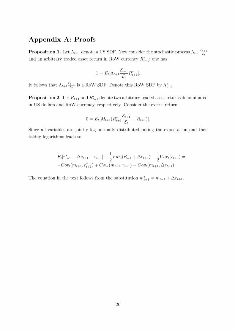
Appendix A: Proofs

Proposition 1. Let Λt+1 denote a US SDF. Now consider the stochastic process Λt+1Et+1

Etand an arbitrary traded asset return in RoW currency R∗t+1; one has

1 = Et[Λt+1Et+1

EtR∗t+1].

It follows that Λt+1Et+1

Et is a RoW SDF. Denote this RoW SDF by Λ∗t+1.

Proposition 2. LetRt+1 andR∗t+1 denote two arbitrary traded asset returns denominated

in US dollars and RoW currency, respectively. Consider the excess return

0 = Et[Mt+1(R∗t+1

Et+1

Et−Rt+1)].

Since all variables are jointly log-normally distributed taking the expectation and then

taking logarithms leads to

Et[r∗t+1 + ∆et+1 − rt+1] +

1

2V art(r

∗t+1 + ∆et+1)−

1

2V art(rt+1) =

−Covt(mt+1, r∗t+1) + Covt(mt+1, rt+1)− Covt(mt+1,∆et+1).

The equation in the text follows from the substitution m∗t+1 = mt+1 + ∆et+1.

20

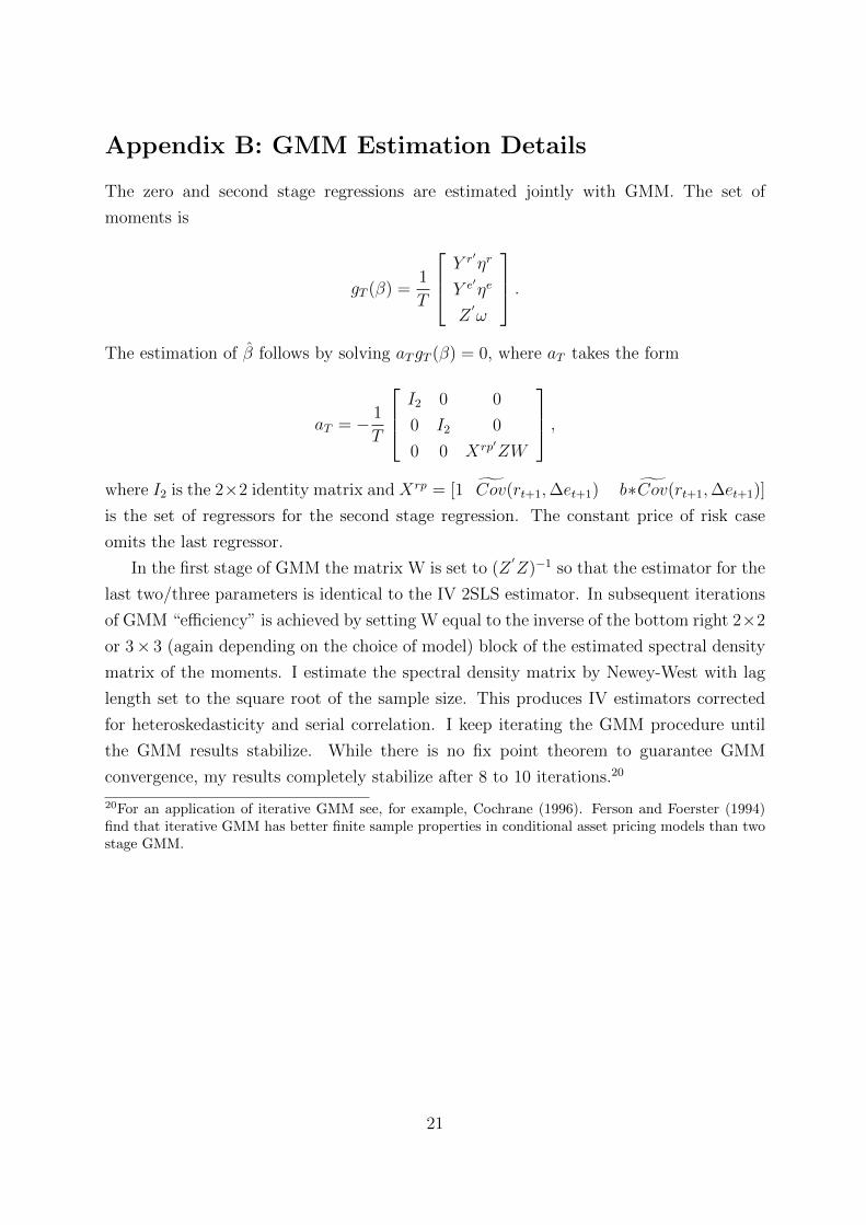
Appendix B: GMM Estimation Details

The zero and second stage regressions are estimated jointly with GMM. The set of

moments is

gT (β) =1

T

Y r′ηr

Y e′ηe

Z′ω

.The estimation of β follows by solving aTgT (β) = 0, where aT takes the form

aT = − 1

T

I2 0 0

0 I2 0

0 0 Xrp′ZW

,where I2 is the 2×2 identity matrix and Xrp = [1 Cov(rt+1,∆et+1) b∗Cov(rt+1,∆et+1)]

is the set of regressors for the second stage regression. The constant price of risk case

omits the last regressor.

In the first stage of GMM the matrix W is set to (Z′Z)−1 so that the estimator for the

last two/three parameters is identical to the IV 2SLS estimator. In subsequent iterations

of GMM “efficiency” is achieved by setting W equal to the inverse of the bottom right 2×2

or 3× 3 (again depending on the choice of model) block of the estimated spectral density

matrix of the moments. I estimate the spectral density matrix by Newey-West with lag

length set to the square root of the sample size. This produces IV estimators corrected

for heteroskedasticity and serial correlation. I keep iterating the GMM procedure until

the GMM results stabilize. While there is no fix point theorem to guarantee GMM

convergence, my results completely stabilize after 8 to 10 iterations.20

20For an application of iterative GMM see, for example, Cochrane (1996). Ferson and Foerster (1994)find that iterative GMM has better finite sample properties in conditional asset pricing models than twostage GMM.

21

Table 1: US Dollar Mean Safety Premium

World Developed Equally WghtMean 0.98% 0.99% 1.18%Stand. Dev 8.06% 8.26% 7.16%Max 10.34% 10.33% 10.21%Max Date Feb-73 Feb-73 Feb-73Min -9.15% -9.16% -8.36%Min Date Nov-78 Nov-78 Oct-08Subcomponents∆e 0.72% 1.12% -2.20%r∗f − rf -0.05% -0.45% 3.13%

Statistics are for monthly currency returns from January 1970 to March 2010. The mean and standard

deviations are annualized, while the Max and Min realizations are on a monthly basis. The Max and Min

date refer to the month when the highest and lowest returns occurred, respectively. The subcomponents ∆e,

and r∗f − rf are the mean log exchange rate change and interest rate differential for each index.

22

Table 2: Zero Stage Regressions: Equity Returns and Exchange Rate Changes

World DevelopedEquity Returns rt+1 rt+1

const. 0.0463 0.0448[2.41] [2.34]

dpt 0.0106 0.0102[2.03] [1.95]

rt 0.1259 0.1227[1.68] [1.67]

R2 0.0238 0.0228Exchange Rate Changes ∆et+1 ∆et+1

const. 0.0004 0.0013[0.29] [1.01]

r∗f,t+1 − rf,t+1 0.1072 0.1330[1.96] [2.22]

∆et 0.0526 0.0415[0.99] [0.81]

R2 0.0133 0.0169

Top panel: regression of the one month return of the equity index on a constant, the logarithm of the

dividend-price ratio for the equity index and the lagged equity index return (see equation (7)). The

explanatory variables are lagged one month. The regression results are provided for both the World and

Developed equity indices. Bottom panel: regression of the one month logarithmic exchange rate change

for the currency index on a constant, the interest rate differential for the currency index and the lagged

logarithmic exchange rate change for the currency index (see equation (8)). The explanatory variables are

lagged one month. The regression results are provided for both the World and Developed currency indices.

The regressions are for the period January 1975-March 2010: 423 observations. The estimates are OLS

and the standard errors are Newey-West with 4 lags. The t-statistic is reported in square brackets.

23

Table 3: First Stage Regressions

Panel A: Exploring covariance predictabilityWorld Developed

Instruments F − Stat χ2 − Stat χ2 p− val F − Stat χ2 − Stat χ2 p− valAll 15.76 94.56 (0.0000) 15.38 92.29 (0.0000)ex dp ratio 14.03 70.16 (0.0000) 13.18 65.88 (0.0000)ex covariance 17.10 85.52 (0.0000) 15.65 78.27 (0.0000)ex volatilities 5.12 20.46 (0.0004) 4.11 16.42 (0.0025)ex return & exch. rate chg. 19.70 78.78 (0.0000) 19.15 76.61 (0.0000)cum int. diff. 14.12 98.85 (0.0000) 13.49 94.44 (0.0000)

Panel B: DetailsWorld Developed

Coeff. × 104 χ2 − Stat χ2 p− val Coeff. × 104 χ2 − Stat χ2 p− valint. diff. -0.60 1.20 (0.2725) -0.44 0.45 (0.5021)

-[1.10] -[0.67]

Panel A: regression of the cross product of residuals from the zero stage regressions for the currency and equity

indices on the set of instruments (see equation (9)). The set of instruments (All) includes: a constant, the

dividend-price ratio for the equity index, the one month lagged return for the equity index, the lagged one-month

return for the equity index, the lagged one-month exchange rate change for the currency index, the lagged two-

month variances for the equity and currency indices, and the lagged three-month covariance of the equity and

currency indices. Robustness checks are performed by excluding subsets of the instruments. For example, the “ex

dp ratio” line reports the regression results for the set of instruments excluding the equity index dividend-price

ratio. The “cum int. diff.” line reports the regression results adding to the set of instruments the interest

rate differential for the currency index. The F-statistic and the Wald χ2 statistic are reported for the null

hypothesis that all coefficients, except the constant, are jointly zero. The p-value for the Wald χ2 test is reported

in parenthesis. Panel B: regression of the cross product of residuals from the zero stage regressions for the currency

and equity indices on a constant and the interest rate differential for the currency index. The point estimate for

the coefficient on the interest rate differential and the corresponding t-statistic, in square brackets, are reported

in addition to the Wald χ2 statistic and corresponding p-value as described above. The regressions are for the

World and Developed equity and currency indices for the period April 1975-March 2010: 420 observations. The

estimates are OLS and the standard errors are Newey-West with lag set at the square root of the sample length

(20 month).

24

Table 4: Instruments Theoretical Sign Predictions

Instrument Definition Predicted Sign(αz) αz

dpt dividend price ratio + +var

′rt lagged equity return volatility + +

var′et lagged exchange rate volatility + +

r∗f,t+1 − rf,t+1 interest rate differential + -rt lagged equity return - -∆et lagged exchange rate change - -Cov′t lagged covariance +/- +

The table reports the set of instruments used in the first stage regressions. The column “Predicted Sign

(αz)” reports the sign that theoretical reasoning predicts for each instrument in the first stage regression.

The theoretical reasoning underlying each sign prediction is discussed in Section IV.C. The column “αz”

reports the estimated sign of each instrument in a first stage regression using the entire set of instruments,

including the interest rate differential. The estimated signs are identical for the World and Developed

indices.

25

Table 5: Second Stage Regressions

World Developedd0 d1 d0 d1

All -0.0028 12.0672 -0.0031 12.4887-[1.45] [3.19] -[1.51] [3.17]

ex dp ratio -0.0042 16.3391 -0.0041 15.4557-[1.59] [2.55] -[1.55] [2.46]

ex covariance -0.0031 13.1771 -0.0035 13.7937-[1.56] [3.16] -[1.64] [3.14]

ex volatilities -0.0005 3.6559 -0.0006 3.8685-[0.22] [0.82] -[0.27] [0.79]

ex return & exch. rate chg. -0.0009 4.6295 -0.0012 5.6272-[0.44] [1.07] -[0.54] [1.21]

cum int. diff. 0.0001 10.2047 0.0006 9.4118[0.03] [2.54] [0.34] [2.28]

Results for the second stage regressions for the case of no time variation in the price of risk. The LHS

variable is the US dollar safety premium: the monthly logarithmic return of investing in the currency index

while funding in US dollars plus the Jensen’s inequality term. The RHS regressors are a constant and the

estimated, in the first stage, conditional covariance between the equity and currency indices returns. See

equation (11) for details. Robustness checks are performed by varying the set of instruments included in the

first stage regressions and, therefore, the resulting estimated covariance that is used as a regressor in the

second stage regression reported here. The set of instruments (All) includes: a constant, the dividend-price

ratio for the equity index, the lagged one-month return for the equity index, the lagged one-month exchange

rate change for the currency index, the lagged two-month variances for the equity and currency indices,

and the lagged three-month covariance of the equity and currency indices. The “ex dp ratio” line, for

example, reports the regression results for the set of instruments excluding the equity index dividend-price

ratio. The “cum int. diff.” line reports the regression results, adding to the set of instruments the interest

rate differential for the currency index. The standard errors are computed using GMM to jointly estimate

the zero, and second stage regressions. The standard errors are based on the Newey-West estimate of the

spectral density matrix in GMM, with lag set to the square root of the sample size (20 lags here), and are

corrected for the uncertainty deriving from using estimated regressors from the zero and first stage. See

Appendix B for details of the estimation.

26

Table 6: Episodes of Crisis

Event PeriodOPEC I, Arab-Israeli War December 1973Franklin National September-October 1974OPEC II, Fed currency Intervention November 1978Iran Hostage Crisis November 1979Silver Wednesday, US-Iran Military Intervention March 1980Latam defaults Early 1980s*1987 crash - Black Monday October 1987Gulf War I September-October 1990Asian Crisis November 1997Russian, LTCM default August-September 1998Dotcom Bust April 2001*9/11 terrorist attack September 2001Worldcom, Enron bankruptcy July-September 2002Credit Cruch, Lehman Default Aug. 2007-Mar. 2009, Oct. 2008

All but episodes marked by * are from Bloom (2009). Bloom uses the US VXO implied volatility index,

backdated using realized volatility, and selects the events as “those with stock-market volatility more than

1.65 standard deviations above the Hodrick Prescott detrended (filter multiplier set at 129,600) mean of the

stock-market volatility series”. The * episodes are added to the list of crises to account for two well known

historical events absent from the list in Bloom (2009). I split the March 1980 event that Bloom completely

attributed to the Iran hostage crisis into two: the November 1979 start of the crisis and the March 1980 US

military intervention that also coincided with the panic following the cornering of the silver market by the

Hunt brothers. Two events from Bloom’s list are not present here. The October-August 1982 “Monetary

policy turning point” has been replaced by the more general label of “Latam defaults” crises to highlight the

protracted period of high volatility without necessarily singling out the monthly evolution of events. The

“Gulf War II” event of March 2003 has been omitted since there was no evidence in my time series of a

market reaction.

27

Figure 1: Equity Total Return Indices: World and Developed

The indices are total return, capital gains plus dividends. The World index includes 23 developed and 22

emerging countries. The Developed index only includes the 23 developed countries. The indices are stock

market capitalization weighted using the MSCI Barra weights. Both indices include the United States.

The two indices are identical for the period 1970-1987 as the emerging countries are assigned a zero

weight, and progressively differ for the period 1988-2010 as the emerging countries’ market capitalization

increases. The Developed index corresponds to the MSCI Barra World index. The World index is built

by using the MSCI Barra World index for the period 1970-1987 and the MSCI Barra All Country World

index for the period 1988-2010. The data are monthly Dec 1969-Mar 2010.

28

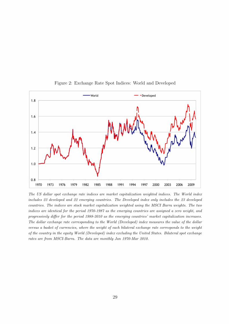
Figure 2: Exchange Rate Spot Indices: World and Developed

The US dollar spot exchange rate indices are market capitalization weighted indices. The World index

includes 23 developed and 22 emerging countries. The Developed index only includes the 23 developed

countries. The indices are stock market capitalization weighted using the MSCI Barra weights. The two

indices are identical for the period 1970-1987 as the emerging countries are assigned a zero weight, and

progressively differ for the period 1988-2010 as the emerging countries’ market capitalization increases.

The dollar exchange rate corresponding to the World (Developed) index measures the value of the dollar

versus a basket of currencies, where the weight of each bilateral exchange rate corresponds to the weight

of the country in the equity World (Developed) index excluding the United States. Bilateral spot exchange

rates are from MSCI-Barra. The data are monthly Jan 1970-Mar 2010.

29

Figure 3: Interest Rate Differential Indices: World and Developed

The interest rate differential indices between the Rest of the World and the US are market capitalization

weighted indices. The World index includes 23 developed and 22 emerging countries. The Developed

index only includes the 23 developed countries. The indices are stock market capitalization weighted

using the MSCI Barra weights. The two indices are identical for the period 1970-1987 as the emerging

countries are assigned a zero weight, and progressively differ for the period 1988-2010 as the emerging

countries’ market capitalization increases. The World (Developed) index measures the weighted interest

rate differential between the US and the countries included in the index, where the weight of each bilateral

interest rate differential corresponds to the weight of the country in the equity World (Developed) index

excluding the United States. Bilateral interest rate differentials are from Maggiori (2010). The data are

monthly Jan 1970-Mar 2010.

30

Figure 4: Mean US Dollar Safety Premium Rolling Window: Start Date to 2010

Plots the average US dollar safety premium for three indices: World, Developed, and Equally Weighted.

The average is taken over a window with a rolling start date and a fixed end date in March 2010.

Therefore, the datapoint for January 1970 is the average for the period Jan 1970-Mar 2010 and the

datapoint for February 1970 is the average for the period Feb 1970-March 2010. The safety premium in

each month is computed as the sum of the logarithmic interest rate differential, the logarithmic exchange

rate change, and the Jensen’s inequality term. The World index includes 23 developed and 22 emerging

countries. The Developed index only includes the 23 developed countries. The indices are stock market

capitalization weighted using the MSCI Barra weights. The two indices are identical for the period 1970-

1987 as the emerging countries are assigned a zero weight, and progressively differ for the period 1988-

2010 as the emerging countries’ market capitalization increases. The Equally weighted index includes all

the 55 countries in the World index and assigns equal weight to each country. The data are monthly Jan

1970-Mar 2010.

31

Figure 5: Mean US Dollar Safety Premium Reverse Rolling Window: 1970 to End Date

Plots the average US dollar safety premium for three indices: World, Developed, and Equally Weighted.

The average is taken over a window with a fixed start date in January 1970 and a rolling end date.

Therefore, the datapoint for March 2010 is the average for the period Jan 1970-Mar 2010 and the

datapoint for February 2010 is the average for the period Feb 1970-Feb 2010. The safety premium in

each month is computed as the sum of the logarithmic interest rate differential, the logarithmic exchange

rate change and the Jensen’s inequality term. The World index includes 23 developed and 22 emerging

countries. The Developed index only includes the 23 developed countries. The indices are stock market

capitalization weighted using the MSCI Barra weights. The two indices are identical for the period 1970-

1987 as the emerging countries are assigned a zero weight, and progressively differ for the period 1988-

2010 as the emerging countries’ market capitalization increases. The Equally weighted index includes all

the 55 countries in the World index and assigns equal weight to each country. The data are monthly Jan

1970-Mar 2010.

32

Figure 6: Ex Post Covariance Cov(rt+1,∆et+1): World Index

The ex post covariance is the product of the residuals of the zero stage regressions:

Cov(rt+1,∆et+1) ≡ εrt+1εet+1, where {εrt+1, ε

et+1} are the residuals of the regressions in equations (7-8).

The zero stage regressions point estimates are obtained by OLS. The resulting time series, the ex-post

covariance, is monthly January 1975-March 2010: 423 observations. The World indices for equity and

currency returns are used in the zero stage regression to estimate the residuals, and consequently the ex

post covariance.

33

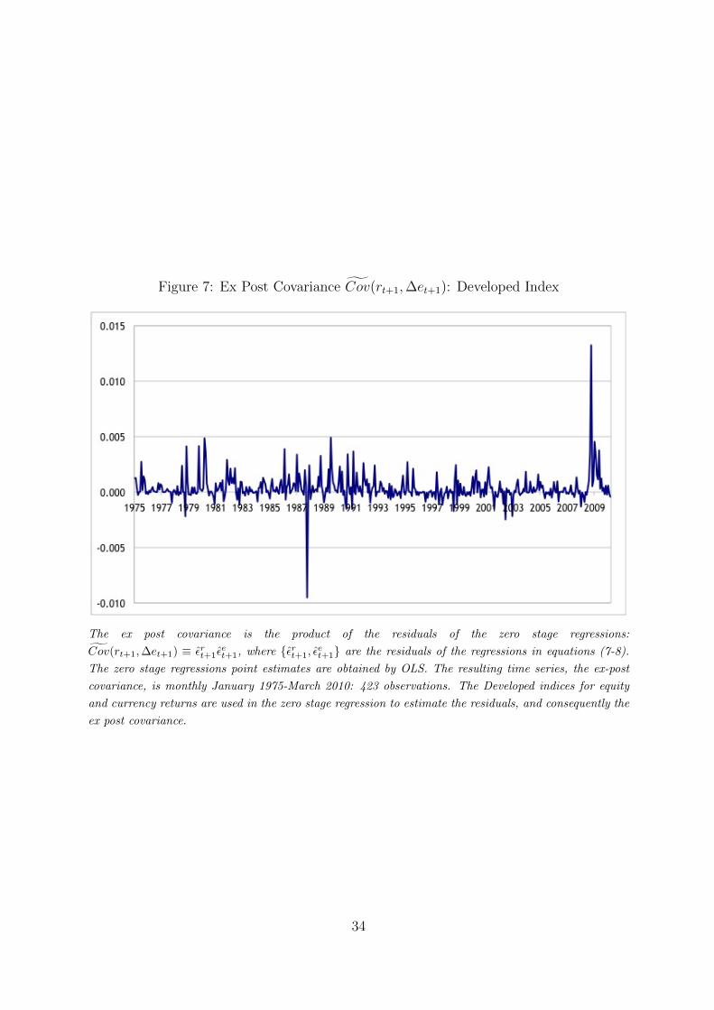
Figure 7: Ex Post Covariance Cov(rt+1,∆et+1): Developed Index

The ex post covariance is the product of the residuals of the zero stage regressions:

Cov(rt+1,∆et+1) ≡ εrt+1εet+1, where {εrt+1, ε

et+1} are the residuals of the regressions in equations (7-8).

The zero stage regressions point estimates are obtained by OLS. The resulting time series, the ex-post

covariance, is monthly January 1975-March 2010: 423 observations. The Developed indices for equity

and currency returns are used in the zero stage regression to estimate the residuals, and consequently the

ex post covariance.

34

Figure 8: Conditional Covariance Cov(rt+1,∆et+1): World Index

The conditional covariance is the fitted value of the first stage regression in equation (9). The first stage

regresses the ex post covariance obtained from the zero stage regressions on a set of instruments. The set

of instruments includes: a constant, the dividend-price ratio for the equity index, the lagged one-month

return for the equity index, the lagged one-month exchange rate change for the currency index, the lagged

two-month variances for the equity and currency indices, and the lagged three-month covariance of the

equity and currency indices. The regression uses the OLS estimator for the World equity and currency

indices for the period April 1975-March 2010: 420 observations.

35

Figure 9: Conditional Covariance Cov(rt+1,∆et+1): Developed Index




return for the equity index, the lagged one-month exchange rate change for the currency index, the lagged


equity and currency indices. The regression uses the OLS estimator for the Developed equity and currency


36

Figure 10: 95% Confidence Band for Conditional Covariance: World Index




return for the equity index, the lagged one-month exchange rate change for the currency index, the

lagged two-month variances for the equity and currency indices, and the lagged three-month covariance

of the equity and currency indices. The regression uses the OLS estimator for the World equity and

currency indices for the period April 1975-March 2010: 420 observations. The confidence band for the

estimate is based on the two sided 95% t-statistic with Newey-West estimates of the standard errors. The

Newey-West lag length is set at the square root of the sample length (20 month).

37

Figure 11: 95% Confidence Band for Conditional Covariance: Developed Index




return for the equity index, the lagged one-month exchange rate change for the currency index, the

lagged two-month variances for the equity and currency indices, and the lagged three-month covariance

of the equity and currency indices. The regression uses the OLS estimator for the Developed equity and

currency indices for the period April 1975-March 2010: 420 observations. The confidence band for the

estimate is based on the two sided 95% t-statistic with Newey-West estimates of the standard errors. The

Newey-West lag length is set at the square root of the sample length (20 month).

38

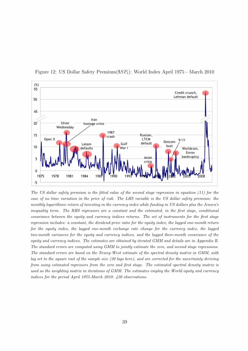
Figure 12: US Dollar Safety Premium($SPt): World Index April 1975 - March 2010

The US dollar safety premium is the fitted value of the second stage regression in equation (11) for the

case of no time variation in the price of risk. The LHS variable is the US dollar safety premium: the

monthly logarithmic return of investing in the currency index while funding in US dollars plus the Jensen’s

inequality term. The RHS regressors are a constant and the estimated, in the first stage, conditional

covariance between the equity and currency indices returns. The set of instruments for the first stage

regression includes: a constant, the dividend-price ratio for the equity index, the lagged one-month return

for the equity index, the lagged one-month exchange rate change for the currency index, the lagged


equity and currency indices. The estimates are obtained by iterated GMM and details are in Appendix B.

The standard errors are computed using GMM to jointly estimate the zero, and second stage regressions.

The standard errors are based on the Newey-West estimate of the spectral density matrix in GMM, with

lag set to the square root of the sample size (20 lags here), and are corrected for the uncertainty deriving

from using estimated regressors from the zero and first stage. The estimated spectral density matrix is

used as the weighting matrix in iterations of GMM. The estimates employ the World equity and currency


39

Figure 13: US Dollar Safety Premium($SPt): Developed Index April 1975 - March 2010

The US dollar safety premium is the fitted value of the second stage regression in equation (11) for

the case of no time variation in the price of risk. The LHS variable is the US dollar safety premium:

the monthly logarithmic return of investing in the currency index while funding in US dollars plus the

Jensen’s inequality term. The RHS regressors are a constant and the estimated, in the first stage,

conditional covariance between the equity and currency indices returns. The set of instruments for

the first stage regression includes: a constant, the dividend-price ratio for the equity index, the lagged

one-month return for the equity index, the lagged one-month exchange rate change for the currency

index, the lagged two-month variances for the equity and currency indices, and the lagged three-month

covariance of the equity and currency indices. The estimates are obtained by iterated GMM and details are

in Appendix B. The standard errors are computed using GMM to jointly estimate the zero, and second

stage regressions. The standard errors are based on the Newey-West estimate of the spectral density

matrix in GMM, with lag set to the square root of the sample size (20 lags here), and are corrected for

the uncertainty deriving from using estimated regressors from the zero and first stage. The estimated

spectral density matrix is used as the weighting matrix in iterations of GMM. The estimates employ the

Developed equity and currency indices for the period April 1975-March 2010: 420 observations.

40

Figure 14: US Dollar Safety Premium($SPt): World Index January 1971 - March 2010

The US dollar safety premium is the fitted value of the second stage regression in equation (11) for the

case of no time variation in the price of risk. The LHS variable is the US dollar safety premium: the

monthly logarithmic return of investing in the currency index while funding in US dollars plus the Jensen’s

inequality term. The RHS regressors are a constant and the estimated, in the first stage, conditional

covariance between the equity and currency indices returns. The set of instruments for the first stage

regression includes: a constant, the dividend-price ratio for the equity index, the lagged one-month return

for the equity index, the lagged one-month exchange rate change for the currency index, the lagged


equity and currency indices. The estimates are obtained by iterated GMM and details are in Appendix B.

The standard errors are computed using GMM to jointly estimate the zero, and second stage regressions.

The standard errors are based on the Newey-West estimate of the spectral density matrix in GMM, with

lag set to the square root of the sample size (20 lags here), and are corrected for the uncertainty deriving

from using estimated regressors from the zero and first stage. The estimated spectral density matrix is

used as the weighting matrix in iterations of GMM. The estimates employ the World equity and currency

indices for the period January 1971-March 2010: 471 observations.

41

Figure 15: US Dollar Safety Premium($SPt): Developed Index January 1971 - March2010

The US dollar safety premium is the fitted value of the second stage regression in equation (11) for

the case of no time variation in the price of risk. The LHS variable is the US dollar safety premium:

the monthly logarithmic return of investing in the currency index while funding in US dollars plus the

Jensen’s inequality term. The RHS regressors are a constant and the estimated, in the first stage,

conditional covariance between the equity and currency indices returns. The set of instruments for

the first stage regression includes: a constant, the dividend-price ratio for the equity index, the lagged

one-month return for the equity index, the lagged one-month exchange rate change for the currency

index, the lagged two-month variances for the equity and currency indices, and the lagged three-month

covariance of the equity and currency indices. The estimates are obtained by iterated GMM and details are

in Appendix B. The standard errors are computed using GMM to jointly estimate the zero, and second

stage regressions. The standard errors are based on the Newey-West estimate of the spectral density

matrix in GMM, with lag set to the square root of the sample size (20 lags here), and are corrected for

the uncertainty deriving from using estimated regressors from the zero and first stage. The estimated

spectral density matrix is used as the weighting matrix in iterations of GMM. The estimates employ the

Developed equity and currency indices for the period January 1971-March 2010: 471 observations.

42

The U.S. Dollar Safety Premium

Documents

Transcript of The U.S. Dollar Safety Premium