The Unscrambler® Appendices: Method References - … · The Unscrambler® Appendices: Method...
45
The Unscrambler® Appendices: Method References This document details the algorithms used in The Unscrambler® 9.6, as well as some statistical measures and formulas. The last section provides some bibliographical references for the methods implemented in The Unscrambler. Contents Notations Used in The Unscrambler................................................................................................................... 3 Model Equations and Algorithms ....................................................................................................................... 4 MLR Equation and Algorithm .......................................................................................................................... 4 MLR Model Equation................................................................................................................................... 5 MLR Algorithm ............................................................................................................................................ 5 Other Methods Based On MLR .................................................................................................................... 5 PCA Equation and Algorithm ........................................................................................................................... 5 PCA Model Equation ................................................................................................................................... 5 PCA Algorithm............................................................................................................................................. 5 Stop criterion in PCA ................................................................................................................................... 6 PCR Equation and Algorithm............................................................................................................................ 7 PCR Model Equation .................................................................................................................................... 7 PCR Algorithm ............................................................................................................................................. 7 PLS Equation and Algorithms ........................................................................................................................... 8 PLS Model Equation .................................................................................................................................... 8 PLS1 Algorithm............................................................................................................................................ 8 PLS2 Algorithm.......................................................................................................................................... 10 Stop criterion in PLS2 ................................................................................................................................ 11 N-PLS Equation and Algorithm ...................................................................................................................... 11 N-PLS Model Equation .............................................................................................................................. 12 tri-PLS Algorithms ..................................................................................................................................... 12 Data Centering, Interactions and Squares ....................................................................................................... 15 Data Centering ................................................................................................................................................ 15 Interactions And Squares................................................................................................................................. 16 Generating Interactions And Squares From Raw Data ............................................................................... 16 How To Make Predictions With Interactions And Squares ........................................................................ 17 Interactions And Squares in Analysis of Effects ........................................................................................ 18 Computation of Main Results ........................................................................................................................... 18 Residuals, Variances and RMSE Computations.............................................................................................. 18 Degrees of Freedom ................................................................................................................................... 18 Calculation of Residuals ............................................................................................................................. 19 Individual Residual Variance Calculations................................................................................................. 19 Total Residual Variance Calculations ........................................................................................................ 20 Explained Variance Calculations................................................................................................................ 20 RMSEC and RMSEP Formula ................................................................................................................... 21
Transcript of The Unscrambler® Appendices: Method References - … · The Unscrambler® Appendices: Method...

The Unscrambler® Appendices: Method References
This document details the algorithms used in The Unscrambler® 9.6, as well as some
statistical measures and formulas.
The last section provides some bibliographical references for the methods implemented
in The Unscrambler.
Contents
Notations Used in The Unscrambler................................................................................................................... 3
Model Equations and Algorithms ....................................................................................................................... 4 MLR Equation and Algorithm .......................................................................................................................... 4
MLR Model Equation ................................................................................................................................... 5 MLR Algorithm ............................................................................................................................................ 5 Other Methods Based On MLR .................................................................................................................... 5
PCA Equation and Algorithm ........................................................................................................................... 5 PCA Model Equation ................................................................................................................................... 5 PCA Algorithm ............................................................................................................................................. 5 Stop criterion in PCA ................................................................................................................................... 6
PCR Equation and Algorithm ............................................................................................................................ 7 PCR Model Equation .................................................................................................................................... 7 PCR Algorithm ............................................................................................................................................. 7
PLS Equation and Algorithms ........................................................................................................................... 8 PLS Model Equation .................................................................................................................................... 8 PLS1 Algorithm............................................................................................................................................ 8 PLS2 Algorithm.......................................................................................................................................... 10 Stop criterion in PLS2 ................................................................................................................................ 11
N-PLS Equation and Algorithm ...................................................................................................................... 11 N-PLS Model Equation .............................................................................................................................. 12 tri-PLS Algorithms ..................................................................................................................................... 12
Data Centering, Interactions and Squares ....................................................................................................... 15 Data Centering ................................................................................................................................................ 15 Interactions And Squares................................................................................................................................. 16
Generating Interactions And Squares From Raw Data ............................................................................... 16 How To Make Predictions With Interactions And Squares ........................................................................ 17 Interactions And Squares in Analysis of Effects ........................................................................................ 18
Computation of Main Results ........................................................................................................................... 18 Residuals, Variances and RMSE Computations.............................................................................................. 18
Degrees of Freedom ................................................................................................................................... 18 Calculation of Residuals ............................................................................................................................. 19 Individual Residual Variance Calculations................................................................................................. 19 Total Residual Variance Calculations ........................................................................................................ 20 Explained Variance Calculations ................................................................................................................ 20 RMSEC and RMSEP Formula ................................................................................................................... 21

The Unscrambler® Appendices: Method References
2 © Copyright CAMO Software AS
SEP and Bias .............................................................................................................................................. 21 Studentized Residuals ................................................................................................................................. 22 Weighting of individual segments in Cross Validation .............................................................................. 22
Two-Variable Statistics Computations ............................................................................................................ 22 Regression Statistics ................................................................................................................................... 22 Correlation Coefficient ............................................................................................................................... 23 RMSED and SED ....................................................................................................................................... 23
Descriptive Statistics Computations ................................................................................................................ 23 Standard Deviation ..................................................................................................................................... 23 Histogram Statistics .................................................................................................................................... 24 Percentiles .................................................................................................................................................. 24
Effects Computations ...................................................................................................................................... 25 Significance Testing Computations ................................................................................................................. 25
Standard Error of the B-coefficients ........................................................................................................... 25 t-values ....................................................................................................................................................... 25 F-ratios........................................................................................................................................................ 26 p-values ...................................................................................................................................................... 26 Multiple Comparisons ................................................................................................................................ 26 Comparison with a Scale-Independent Distribution (COSCIND) .............................................................. 26 Higher Order Interaction Effects (HOIE) ................................................................................................... 27
Leverage Calculations ..................................................................................................................................... 27 High Leverage and Outlier Detection.............................................................................................................. 28 Warning Limits and Outlier Warnings ............................................................................................................ 29 Hotelling T2 Computations ............................................................................................................................. 31 Deviation in Prediction .................................................................................................................................... 32 Classification Statistics ................................................................................................................................... 32
Sample to Model Distance .......................................................................................................................... 32 Model Distance ........................................................................................................................................... 33 Discrimination Power ................................................................................................................................. 33 Modeling Power ......................................................................................................................................... 34 Class Membership Limits ........................................................................................................................... 34
Computation of Transformations ..................................................................................................................... 35 Smoothing Methods ........................................................................................................................................ 35 Normalization Equations ................................................................................................................................. 35 Spectroscopic Transformation Equations ........................................................................................................ 36 Multiplicative Scatter Correction Equations ................................................................................................... 36 Added Noise Equations ................................................................................................................................... 37 Differentiation Algorithm................................................................................................................................ 37
Mixture and D-Optimal Designs ....................................................................................................................... 38 Shape of the Mixture Region ........................................................................................................................... 38
Notations .................................................................................................................................................... 38 Simplex Region .......................................................................................................................................... 38 Upper/Lower Bound Consistency............................................................................................................... 38
Computation of Candidate Points for a D-Optimal Design ............................................................................. 39 D-Optimal Selection of Design Points ............................................................................................................ 39
Bibliographical References ................................................................................................................................ 40 About Statistics and Multivariate Data Analysis ............................................................................................. 40 About Martens’ Uncertainty Test .................................................................................................................... 41 About Three-way Data and Tri-PLS ............................................................................................................... 42 About Experimental Design ............................................................................................................................ 42 About Numerical Algorithms .......................................................................................................................... 43
Index .................................................................................................................................................................... 43

The Unscrambler® Appendices: Method References
© Copyright CAMO Software AS 3
Notations Used in The Unscrambler The tables below list the general notation and the nomenclature used throughout this
manual.
General notation
Symbol Description
v Scalar variable
[ ]v = v v vN1 2 … (1:N) Vector, line or column, with N elements
ν ι The ith element in the vector v
vT Vector v transposed
(1:I, 1:J) Matrix with I rows and J columns
m M i jij = ( , )
The ith element in the jth column of M. As a general rule, the parenthesis notation is used in connection with “named” matrices (eg. DescMean), whereas the index notation is used where needed for readability (eg. xik instead of xRaw(i, k) ).
M M( , j)(j) = •
The jth column vector in M
MT
The matrix M transposed
T (i, j)k The ith element in the jth column of the kth slice of a 3-dimensional matrix T
Nomenclature
Symbol Description
a, A Principal component (PC) number and No. of PCs
b0 ,b0 Intercept (single, vector)
b, b, B Regression coefficients (estimated) ***
C 0 if model is un-centered, 1 if model is centered
d Number of degrees of freedom
Ea X-residuals for a model using (a) PCs
f, Fa Y-residuals for a model using (a) PCs
h, H Leverages of samples (single, matrix)
i, I Sample number and No. of samples
j, J Y-variable number and No. of Y-variables
k, K X-variable number and No. of X-variables
N Number of elements
p, P X-Loadings (vector, matrix)
q, Q Y-Loadings (vector, matrix)
ß B-coefficient (exact)
t, T Scores (vector, matrix)
u, U Preliminary scores (vector, matrix)

The Unscrambler® Appendices: Method References
4 © Copyright CAMO Software AS
Symbol Description
w, W X-Loading weights (vector, matrix)
x, x
Mean value in x or X
x, x, X x-values (single, vector, matrix)
y, y
Mean value in y or Y
$y
Predicted value of y
y, y, Y y-values (single, vector, matrix)
Model Equations and Algorithms The equations used in the different analysis methods are shown here.
The Unscrambler contains the algorithms for MLR, PCA, PCR, and PLS.
For further reading about algorithms and computations in general we refer you to the
texts by Golub and Press (see section The D-optimal selection of a design point is based
on the algorithm DOPT (MILLER and NGUYEN, 1994).
The FORTRAN algorithm DOPT is used to D-optimally select a number of design
points from a set of candidate points. The design points are chosen so that the
determinant of X'X is maximized (X is the design point matrix).
DOPT:
1. Start with a default set of design points, or else generate a random set.
2. Calculate X'X for the selected points.
3. As long as there is improvement do:
a. Find the selected point and unselected candidate point
which will improve the X'X determinant the most.
b. Exchange the points, and calculate new X'X.
Bibliographical References).
MLR Equation and Algorithm
MLR is used as common basis for three analysis methods used in The Unscrambler:
• Multiple Linear Regression;
• Analysis of Effects;
• Response Surface Analysis.

The Unscrambler® Appendices: Method References
© Copyright CAMO Software AS 5
MLR Model Equation
The general model equation, which relates a response variable to several predictors by
means of regression coefficients, has the following shape:
y x x x fK K= + + + + +β β β β0 1 1 2 2…
or, in matrix notation : y = X b + f.
MLR Algorithm
The SVD (Singular Value Decomposition) algorithm is the most widely used algorithm
to compute the estimated regression coefficients for MLR.
Other Methods Based On MLR
Analysis of Effects and Response Surface are based on MLR computations, and
algorithms will not be shown explicitly for these methods here.
PCA Equation and Algorithm
The algorithms used in The Unscrambler for PCA, PCR and PLS are described in
“Multivariate calibration” by Martens & Næs (Wiley 1991, ISBN 0471930474). The
following descriptions of the PCA, PCR and PLS algorithms are reproduced from the
book, with the permission of John Wiley & Sons Ltd.
PCA Model Equation
The general form of the PCA model is:
X T P ET= ⋅ +
Usually the PCA model is centered, which gives:
X 1 x T P Emean (A) (A)
T
(A)= ⋅ + ⋅ +
Another way to put this is:
x x t p eik mean k ia ka ik A
a
A
= + +=∑, ( )
1
PCA Algorithm
The PCA computations implemented in The Unscrambler are based on the NIPALS
algorithm.

The Unscrambler® Appendices: Method References
6 © Copyright CAMO Software AS
The NIPALS algorithm for PCA
The algorithm extracts one factor at a time. Each factor is obtained iteratively by
repeated regressions of X on scores $t to obtain improved $p and of X on these $p to
obtain improved $t . The algorithm proceeds as follows:
Pre-scale the X-variables to ensure comparable noise-levels. Then center the X-
variables, e.g. by subtracting the calibration means ′x , forming X0. Then for factors a =
1, 2, ..., A compute $ta and $p
a from Xa-1:.
Start:
Select start values. e.g. $t a = the column in Xa-1 that has the highest remaining sum of
squares.
Repeat points i) to v) until convergence.
i) Improve estimate of loading vector $p a for this factor by projecting the matrix Xa-1 on
$t a , i.e.
$ ($ $ $′ = ′ ′p t t ) t X-1
a a a a a-1
ii) Scale length of $pa to 1.0 to avoid scaling ambiguity:
$ $ ( $ $ ) .p p p pa a a a= ′ −0 5
iii) Improve estimate of score $t a for this factor by projecting the matrix Xa-1 on $p a:
$ $ ( $ $ )t X p p pa a 1 a a a= ′−
−1
iv) Improve estimate of the eigenvalue $τ a:
$ $ $τ a a a= ′t t
v) Check convergence: If $τa minus $τ
a in the previous iteration is smaller than a certain
small pre-specified constant, e.g. 0.0001 times $τa, the method has converged for this
factor. If not, go to step i).
Subtract the effect of this factor:
X X t pa a a a= − ′−1
$ $
and go to Start for the next factor
Stop criterion in PCA
Some users of Unscrambler versions prior to 7.5 have reported that the stop criterion has
been too loose in some situations compared to e.g. Matlab results. As a result, in The
Unscrambler 7.5 and later versions the stop criterion has been changed to ||told-t|| < 1.e-
12, giving more strict orthogonality in scores and loadings. The maximum number of
iterations has been changed as well, from 50 to 100.

The Unscrambler® Appendices: Method References
© Copyright CAMO Software AS 7
PCR Equation and Algorithm
PCR is based on PCA and MLR.
PCR Model Equation
The general form of the PCR model is:
X T P ET= ⋅ + and y T b f= ⋅ +
where the decomposition of the X matrix is computed using PCA and the b-coefficients
are computed using MLR.
PCR Algorithm
PCR is performed as a two step operation:
4. First X is decomposed by PCA, see PCA Algorithm.
5. Then the principal components regression is obtained by
regressing y on the $t ’s.
A Principal Component Regression of J different Y-variables on K X-variables is
equivalent to J separate principal component regressions on the same K X-variables (one
for each Y-variable). Thus we here only give attention to the case of one
single Y-variable, y.
The principal component regression is obtained by regressing yyyy on the $t ’s obtained from
the PCA of X. the regression coefficients $b for each y can according to equation (1) be
written
(1) $ $ $b Pq=
where X-loadings
{ }$ $ , , , , , , ,P p and= = =ka
k K a A1 2 1 2K K
represent the PCA loadings of the A factors employed, and Y-loadings
$ ( $ , , $ )q q q A= ′1 K
are found the usual way by least squares regression of y on $T from the model y=Tq+f.
Since the scores in $T are uncorrelated, this solution is equal to
$ ( ( $ )) $q diag T y= ′−
11τ a
Inserting this in (1) and replacing $T by XP$ , the PCR estimate of b can be written as
$ $ ( ( $ )) $b P diag P X ya
= ′ ′1 τ
which is frequently used as definition of the PCR (Gunst and Mason, 1979).

The Unscrambler® Appendices: Method References
8 © Copyright CAMO Software AS
When the number of factors A equals K, the PCR gives the same $b as the MLR. But the
X-variables are often intercorrelated and somewhat noisy, and then the optimal A is less
than K:
In such cases MLR would imply division by eigenvalues $τa close to zero, which makes
the MLR estimate of b unstable. In contrast PCR attains a stabilized estimation of b by
dropping such unreliable eigenvalues.
PLS Equation and Algorithms
PLS decomposes X and Y simultaneously. It is found in two versions:
• PLS2 is the most general and handles several Y-variables
together;
• PLS1 is a simplification of the PLS algorithm made
possible in the case of only one Y-variable.
PLS Model Equation
The general form of the PLS model is:
X T P ET= ⋅ + and FBTY +⋅=
PLS1 Algorithm
Orthogonalized PLSR algorithm for one Y-variable: PLS1.
Calibration:
C 1C 1C 1C 1 The scaled input variables X and y are first centered, e.g.
X X x and y y0 0
1 1= − ′ = − y
Choose Amax to be higher than the number of phenomena expected in X.
For each factor a = 1,..., Amax perform steps C 2.1 - C 2.5:
C 2.1C 2.1C 2.1C 2.1 Use the variability remaining in y to find the loading weights wa, using LS and
the local 'model'
X y w Ea 1 a 1 a− −= ′ +
and scale the vector to length 1. The solution is
$w X ya a 1 a 1
c= ′ − −
where c is the scaling factor that makes the length of the final $wa equal to 1,
i.e.

The Unscrambler® Appendices: Method References
© Copyright CAMO Software AS 9
ca 1 a 1 a 1 a
= ′ ′− − − −−( ) .y X X y
1
0 5
CCCC 2.22.22.22.2 Estimate the scores $ta using the local 'model'
X t w Ea− = ′ +1 a a$
C 2.4C 2.4C 2.4C 2.4 Estimate the chemical loading qa using the local ‘model’
y t fa 1 a a
q− = +$
which gives the solution
$ $ $ $qa a 1 a a a= ′ ′−y t t t
C 2.5C 2.5C 2.5C 2.5 Create new X and y residuals by subtracting the estimated effect of this factor:
$ $ $E X t p= − ′−a 1 a a
$ $ $f y t q= −−a 1 a a
Compute various summary statistics on these residuals after a factors, summarizing $eik
over objects i and variables k, and summarizing $fi over i objects (see Chapters 4 and 5).
Replace the former X a−1 and ya−1 by the new residuals $E and $f and increase a by 1, i.e.
set
X Ea = $
y fa= $
a = a + 1
C 3C 3C 3C 3 Determine A, the number of valid PLS factors to retain in the
calibration model.
C 4C 4C 4C 4 Compute $b0 and $b for A PLS factors, to be used in the predictor $
$ $y X b= +1 0b
(optional, see P4 below)
$ $ ( $ $ ) $b W P W q= ′ −1
$ $b y0= − ′x b
Prediction:
Full predictionFull predictionFull predictionFull prediction
For each new prediction object i = 1,2,... perform steps P1 to P3, or alternatively, step
P4.
P1P1P1P1 Scale input data xi like for the calibration variables. Then compute

The Unscrambler® Appendices: Method References
10 © Copyright CAMO Software AS
′ = ′ − ′x x xi,0 i
where x is the center for the calibration objects.
For each factor a = 1 ... A perform steps P 2.1 - P 2.2.
P 2.1P 2.1P 2.1P 2.1 Find $ti,a according to the formula in C 2.2 i.e.
$ $ti,a i,a 1 a= ′ −x w
P 2.2P 2.2P 2.2P 2.2 Compute new residual x x pi,a i,a 1 ia a
t= − ′−$ $
If a < A, increase a by 1 and go to P 2.1. If a = A, go to P 3.
P 3P 3P 3P 3 Predict yi by $ $ $y y t qi ia a
a 1
A
= +=∑
Compute outlier statistics on xiA and $t i (Chapters 4 and 5).
Short predictionShort predictionShort predictionShort prediction
P 4P 4P 4P 4 Alternatively to steps P 1 - P 3, find $y by using $b0 and $b in C 4,
i.e.
$ $ $y bi 0= + ′x b
i
Note that P and Q are not normalized. T and W are normalized to 1 and orthogonal.
PLS2 Algorithm
Simultaneous PLSR calibration for several Y-variables: PLS2.
If we replace vectors y, f, and q in the PLS1 algorithm by matrices Y(dim I*J), F(dim
I*J) and Q(dim J*A), the calibration in PLS2 is almost the same as for the
orthogonalized PLS1.
The exceptions are that ya−1 in C 2.1 is replaced by a temporary Y-score for this factor,
$ua and that two extra steps are needed between C 2.4 and C 2.5:
C 2.1C 2.1C 2.1C 2.1 Use the temporary Y-factor $ua that summarizes the remaining variability in Y,
to find the loading-weights $wa by LS, using the local 'model'
X u w Ea 1 a a− = ′ +$
and scale the vector to length 1. The LS solution is
$ $w X u
a a 1 ac= ′−

The Unscrambler® Appendices: Method References
© Copyright CAMO Software AS 11
where c is the scaling factor that makes the length of the final $wa equal to 1, i.e.
ca a 1 a 1 a
= ′ ′− −−( $ $ ) .u X X u 5
The first time this step is encountered, $ua has been given some start values, e.g. the
column in Ya−1 with the largest sum of squares.
The following two extra stages are then needed between C 2.4 and C 2.5:
C 2.4bC 2.4bC 2.4bC 2.4b
Test whether convergence has occurred, by e.g. checking that the elements have no
longer changed meaningfully since the last iteration.
C 2.4cC 2.4cC 2.4cC 2.4c
If convergence is not reached, then estimate temporary factor scores u a using the 'model'
Y u q Fa 1 a a− = ′ +$
giving the LS solution
$ $ ( $ $ )u Y q q qa a 1 a a a= ′−
−1
and go to C 2.1.
If convergence has been reached, then go to step 2.5.
The expression for $B is the same in this PLS2 algorithm as in the PLS1 algorithm, i.e.
$ $ ( $ $ ) $B W P W Q= ′ ′−1
and
′ = ′ − ′b y x B0
$
Stop criterion in PLS2
Some users of Unscrambler versions prior to 7.5 have reported that the stop criterion has
been too loose in some situations compared to e.g. Matlab results. As a result, in The
Unscrambler 7.5 and later versions the stop criterion has been changed to ||told-t|| < 1.e-
12, giving more strict orthogonality in scores and loadings. The maximum number of
iterations has been changed as well, from 50 to 100.
N-PLS Equation and Algorithm
N-PLS or tri-PLS is the new method that allows you to build a model where a matrix of
responses (Y) is expressed as a function of a 3-way array of predictors.

The Unscrambler® Appendices: Method References
12 © Copyright CAMO Software AS
N-PLS Model Equation
The general form of the N-PLS model is:
(2) (1) TX T (W W ) E= ⋅ +o and FBTY +⋅=
where X is unfolded to a matrix and o is the Khatri-Rao product (columnwise
Kronecker product).
tri-PLS Algorithms
The tri-PLSR algorithm for one or several Y-variables using three-way X (tri-PLS1 and
tri-PLS2 regression) is given hereafter.
Note: Step numbering has been adjusted so as to be consistent with the numbering in the
PLS1 and PLS2 algorithms.
For tri-PLS1, the matrix Y has only one column. Below the three-way X(dim I*K*L)
has been rearranged to a matrix X with I rows and KL columns (unfolded/matricized).
Calibration:
C 1C 1C 1C 1 The scaled input variables X and Y are first centered, i.e.
0 0X X - 1x' and Y Y - 1y= =
Choose Amax to be higher than the number of phenomena expected in X.
For each factor a = 1,..., Amax perform steps C 2.1 - C 2.5:
C 2.1C 2.1C 2.1C 2.1 Use the variability remaining in Y to find the loading weights wa, using LS
and the local 'model' below. For each component there is a weight vector for the first
variable mode, w(1)(dim K*A) and one for the second variable mode w
(2)(dim L*A)
(2) (1)
0 a a aX u (w w )' E= ⊗ +
Scale the weight vectors to length 1. This model is a trilinear model similar to the two-
way bilinear analogue. The solution is obtained from a one-component PCA model of
the matrix Z(dim K*L) which is the ‘inner’ product of X and u. Hence the element k,l of
Z is the inner product of u and the column in X with variable mode 1 index k and
variable mode 2 index l. The normalized score vector of the one-component PCA model
of Z is equal to (1)
aw and the loading vector to (2)
aw . From the two weight vectors, a
combined weight vector wa applicable for the rearranged X data, is defined as
(2) (1)
a a aw w w )= ⊗ .
This is the Kronecker tensor product which is a larger matrix formed from all possible
products of elements of (1)
aw with those of (2)
aw .

The Unscrambler® Appendices: Method References
© Copyright CAMO Software AS 13
The first time this step is encountered, $ua has been given some start values, e.g. the
column in Ya−1 with the largest sum of squares.
C 2.2C 2.2C 2.2C 2.2 Calculate the scores $ta using the local 'model'
X t w Ea− = ′ +1 a a$
which has the solution
a 0 at X w=
C 2.4C 2.4C 2.4C 2.4 Estimate the chemical loading qa using the local ‘model’
a-1 a aˆY t q F= +
which gives the solution
a a-1 a a aˆ ˆ ˆq Y 't / t ' t= .
Subsequently aq is normalized to length 1 (unlike in two-way PLS regression).
C 2.4cC 2.4cC 2.4cC 2.4c Estimate factor scores u a using the 'model'
Y u q Fa 1 a a− = ′ +$
giving the LS solution
$ $ ( $ $ )u Y q q qa a 1 a a a= ′−
−1
C 2.4dC 2.4dC 2.4dC 2.4d Test whether convergence has occurred by e.g. checking that the elements
have no longer changed significantly since the last iteration. For tri-PLS1 where there is
only one Y-variable, convergence is reached immediately after first iteration when ua is
initialized as ya-1. The stopping criterion may be 10-6, or less, as desired.
Check convergence: if | ua – ua-1 | < criterion, convergence has been reached. Then go to
step 2.5 else go to C 2.1.
C 2.5aC 2.5aC 2.5aC 2.5a Determine inner-relation regression coefficients for estimating ua from ta. Due to non-orthogonal X-scores include all scores from 1 to a.
inner -1
a 1-a 1-a 1-a aˆ ˆ ˆ ˆ ˆb =(T 'T ) T 'u
Note that there is a unique set of a inner relation coefficients for each component.
Hence, for all components these are held in a matrix (dim A*A) which has zeros on each
lower triangular part.

The Unscrambler® Appendices: Method References
14 © Copyright CAMO Software AS
C 2.5bC 2.5bC 2.5bC 2.5b Calculate core array. The core array is used for building the X model to obtain
X-residuals. This model is a so-called Tucker structure where the core is used to relate
the scores and weights using the model
(2) (1)
1 a a 1-a 1-a aˆ ˆ ˆX =T G (W W )' E− ⊗ +
The core is determined in a least squares sense from
1
a 0 aˆvecG =(S'S) S'vecX E− +
where vecGa is the core array Ga(dim a*a*a) rearranged to a vector and vecX0 is defined
likewise. The matrix S is defined as
(2) (1)
1-a 1-a 1 aˆS =W W T −⊗ ⊗
Note that X-residuals are not used in the algorithm, but only for diagnostic purposes.
C 2.5cC 2.5cC 2.5cC 2.5c Create new y-residuals by subtracting the estimated effect of this factor
a-1 1-a 1-a,a aˆ ˆ ˆ ˆF = Y T B q'−
Replace the former Ya-1 by the new residuals F and increase a by 1, i.e. set
aˆY = F
a = a + 1
C 3C 3C 3C 3 Determine A, the number of valid PLS factors to retain in the calibration
model.
C 4C 4C 4C 4 Compute 0
B and B for A PLS factors, to be used in the predictor
0ˆ ˆ ˆY=B XB+
(optional, see P4 below)
inner ˆˆ ˆ ˆB=WB Q
and
0ˆ ˆB Y' X'B= −
Note that Q and W are normalized to 1 and orthogonal.
Prediction:
Full predictionFull predictionFull predictionFull prediction

The Unscrambler® Appendices: Method References
© Copyright CAMO Software AS 15
The three-way X(dim I*K*L) is rearranged to a matrix X with I rows and KL columns
(unfolded/matricized).
Perform steps P1 to P4, or alternatively, step P5.
P1P1P1P1 Scale input data X like for the calibration variables. Then compute
0X X - 1x'=
where x is the center for the calibration objects.
P2P2P2P2 Find T according to the formula
T XW=
P3P3P3P3 Predict Y by
ˆˆ ˆ ˆY = TBQ'
P4P4P4P4 Calculate X-residuals
(2) (1)
0ˆˆ ˆ ˆE = X -TG(W W )'⊗
Compute outlier statistics on xiA and $ti (Chapters 4 and 5).
ShortShortShortShort predictionpredictionpredictionprediction
P5P5P5P5 Alternatively to steps P1 – P4, find Y by using 0B and B in C 4, i.e.
0ˆ ˆ ˆY=B XB+
Data Centering, Interactions and Squares Data centering and computation of interactions and squares are done automatically in
The Unscrambler, according to the formulas given in the sections that follow.
Data Centering
The center value is either 0 (origo) or the x- or y-variable mean:

The Unscrambler® Appendices: Method References
16 © Copyright CAMO Software AS
xCent xRaw
yCent yRaw
( , ) ( , )
( , ) ( , )
1
01
1
01
1
1
k
Ii k
j
Ii j
i
I
i
I
=
=
=
=
∑
∑
if model center is origo
if model center is mean
if model center is origo
if model center is mean
Interactions And Squares
PCA, PCR, PLS, MLR, Classification, Prediction, Response Surface and Analysis of
Effects are based on X-Variable Sets which may include Interaction and Square effects.
These special X-variables are not stored together with the raw data in your table; they
are generated “on the fly” from your data selection, each time you make a new model.
Generating Interactions And Squares From Raw Data
In all cases, except Analysis of Effects, interaction and square effects are calculated
from standardized main predictor variables (X-variables). If xAB is the interaction term
of variables A and B, and xA2 is the square term of variable A, then:
( ) ( )x (i) = WeightI&S(A) x CentI&S(A) WeightI&S(B) x CentI&S(B)AB i,A i,B⋅ − ⋅ ⋅ −
( )( )x (i) WeightI&S(A) x CentI&S(A)A i,A
2
2 = ⋅ −
where
CentI& S(k)1
Ix
C
i,k
i {calibrationsamples}
=∈∑
and
( )WeightI& S(k)
1
1
I 1x CentI& S(k)
c
i,k
2
i {calibrationsamples}
=
−−
∈∑
The standardized main variables are only used in calculating the interaction and square
effects. The analysis is otherwise based on raw data values of the main variables.
Centering and weighting options specific to each analysis (used in PLS, PCR, PCA and
Response Surface) are applied to the data, according to user choice, after the interaction
and square effects have been generated.

The Unscrambler® Appendices: Method References
© Copyright CAMO Software AS 17
How To Make Predictions With Interactions And Squares
The strategy varies depending on the type of model to be used.
Predictions From PCR And PLS Models
The Unscrambler takes care of predictions from PCR or PLS models with the Predict
task. If the X-Variable Set your regression model is based on, contains any interactions
and squares, you will get correct results provided that you select the same X-Variable
Set for prediction.
SIMCA Classification
The same applies to a Classification with PCA models based on an X-Variable Set
containing interactions and squares.
Predictions from MLR and Response Surface Models
MLR and Response Surface models, on the other hand, cannot be used for automatic
predictions. If you want to predict response values for new samples, you have to do it
manually, using a prediction equation based on the regression coefficients (B-
coefficients). If the source model contains any interaction and square effects, you have
to generate these variables from your raw data using the CentI&S and WeightI&S values
stored together with the model results.
In practice, here is how to do it:
1- Build your model and save it.
2- Import the regression coefficients (stored in matrices B0 and B of your model result
file) into a new data table.
3- Import the CentI&S and WeightI&S matrices from your model result file into
another data table.
4- Copy those numbers to a worksheet (e.g. Excel), and prepare a formula for
computing the interactions and squares from your raw data. Use the equations given
above for XAB and XA2.
5- Prepare a prediction formula which combines the imported regression coefficients
and the values of the main X-variables, of XAB and XA2.
Note: In Response Surface analysis, the main predictor variables are centered before
calculating the B-coefficients. The same must be done to main variables which are used
in prediction.

The Unscrambler® Appendices: Method References
18 © Copyright CAMO Software AS
Interactions And Squares in Analysis of Effects
Analysis of Effects uses coded levels of the X-variables instead of raw values (see
section Descriptive Statistics Computations). Interaction and square effects are
calculated directly from the coded values, without any standardization.
Computation of Main Results This section gives the principles and formulas applied in the main computations performed by The
Unscrambler: various result matrices and warnings.
Residuals, Variances and RMSE Computations
Residuals are computed as the difference between measured values and fitted values,
and are thereafter combined into various kinds of error measures. Variances and
RMSEC/RMSEC are the most commonly used.
In The Unscrambler, variances are usually computed with a correction for the number of
residual degrees of freedom.
Degrees of Freedom
The residual Degrees of Freedom (d.f.) are taken into account in the computation of
conservative variance estimates.
The number of Degrees of Freedom varies according to the context. The table below
explains how the Degrees of Freedom are determined in The Unscrambler.
Degrees of Freedom
Degrees of
freedom
Equation
d 1 [ ]( )1
KK I KC a m ax I C , Kc c− − ⋅ −
d 2 I c
d 3 IK a
Kpr
−
d 4 I C ac − −
d 5 I pr
d 6 [ ]( )1
IKI KC a max I C, K
c
c c− − ⋅ −
d 7 K a−
d 8 ( )( )1
IJ I C a
c
c − −

The Unscrambler® Appendices: Method References
© Copyright CAMO Software AS 19
d 9 J
d10 K
Note: Not all statistical and multivariate data analysis packages correct the variation in
the data for degrees of freedom. And there are different ways of doing it. The variances
calculated in The Unscrambler may therefore differ somewhat from other packages. You
may multiply the result by the adequate “d” factor if you wish to get the uncorrected
variance.
Calculation of Residuals
The residuals are calculated as the difference between the actual value and the predicted
or fitted value.
f y y i I j Jij ij ij C, ,( $ ) ,Cal C al , == − =1 1K K
Residuals are calculated for X (Eix) and Y(Fiy).
Individual Residual Variance Calculations
Residual variance is defined as the mean squared residual corrected for degrees of
freedom. Residual variances are calculated for models incorporating an increasing
number of PCs, a = 0…A.
Replace elements in the equations below with the correct combination as found (CV =
Cross Validation; TS = Test Set validation; LC = Leverage Correction):
Elements of the individual Residual Variance calculations
Description ResVar CV & TS
LC n, N R
Variance per X-variable
calibration samples
ResXCalVar d2 d2 i, IC Eix
Variance per X-variable
validation samples
ResXValVar d3 d1 i, Ipr Eix
Variance per Y-variable
calibration samples
ResYCalVar d2 d2 i, IC Fiy
Variance per Y-variable
validation samples
ResYValVar d5 d2 i, Ipr Fiy
Variances per samples in X
calibration samples
ResXCalSamp d10 d10 k, K Eix
Variances per samples in X
validation samples
ResXValSamp d7 d10 k, K Eix
Variances per samples in Y ResYCalSamp d9 d9 j, J Fiy

The Unscrambler® Appendices: Method References
20 © Copyright CAMO Software AS
calibration samples
Variances per samples in Y
validation samples
ResYValSamp d9 d9 j, J Fiy
MLR: Variance per Y-variable
calibration samples
ResYCalVar d4 d4 i, IC Fiy
MLR: Variances per samples in Y
calibration samples
ResYCalSamp d8 d8 j, J Fiy
ResVar(a, z)1
d
R
(1 H )
a
2
i
2=
−=∑n
N
1
The term ( )1 H i
2
− is used only when the calibration samples are leverage corrected. For
cross validation and test set this equation is used:
ResVar(a, z)1
dR a
2==∑n
N
1
Total Residual Variance Calculations
The total residual variance is calculated from the residual variance for a PCs, a = 0…A.
ResTot(a, )1
NResVar(a, n)
n 1
N
• ==∑
The different cases of Total Residual Variance matrices are listed below.
Elements of the Total Residual Variance calculations
ResTot n,N ResVar
ResXCalTot k, K ResXCalVar
ResXValTot k, K ResXValVar
ResYCalTot j, J ResYCalVar
ResYCalTotCVS j, J ResYCalVar for each CVS segment
ResYValTot j, J ResYValVar
ResYValTotCVS j, J ResYCalVar for each CVS segment
Explained Variance Calculations
The explained variance for PC a is expressed in %, and is calculated from the residual
variance as:

The Unscrambler® Appendices: Method References
© Copyright CAMO Software AS 21
( )
( )
V
V a
V a V a
V V a V a
V a V a
a A
Exp
Exp
Res Res
ResRes Res
Res Res
,
if
if
,
( )
( )
( ) ( )
( ) ( ) ( )
( ) ( )
0 0
1
0
0
1 0
1 0
1
=
=
− −
− − >
− − ≤
= K
where VRes is any of the residual variance matrices listed in Individual Residual Variance
Calculations and VExp is the corresponding explained variance matrix.
Cumulative explained variances after a PCs are also computed, according to the
following equation:
( ) ( ) ( )
( )V a
V V
VExp cum
s s a
s
,
Re Re
Re
=−
0
0
They are also expressed as a percentage.
RMSEC and RMSEP Formula
The Root Mean Square Error is calculated for the prediction or validation samples
(RMSEP) and for the calibration samples (RMSEC).
RMSEC (all validation methods):
RMSEC1
yWeightResYCalVar=
RMSEP (leverage correction and test set validation):
RMSEP1
yWeightResYValVar=
RMSEP (cross validation):
RMSEPItot yWeights2
Fiys(i, j)2
i 1
Is
s 1
Nseg=
=∑
=∑
1 1
SEP and Bias
Bias is the average value of the difference between predicted and measured values.

The Unscrambler® Appendices: Method References
22 © Copyright CAMO Software AS
Bias = −=∑1
1I
y yi i
i
I
( $ )
SEP (Standard Error of Prediction) is the standard deviation of the prediction residuals.
SEP Bias=−
− −=∑1
12
1I
y yi i
i
I
( $ )
Studentized Residuals
Residuals can be expressed raw, or studentized. Studentization takes into account the
standard deviation and sample leverage, so that studentized residuals can be compared to
each other on a common scale.
rf
hi I j Jij
ij
j i
=−
=,
$,
Cal , =
σ 11 1K K
Weighting of individual segments in Cross Validation
With the assumption that the validation should reflect the prediction error for future
samples, one has to decide whether samples that are kept out in the current segment
should be re-centered and/or re-weighted based on mean and standard deviation for the
samples in the segment.
The Unscrambler has in previous versions both re-centered and re-weighted in each
cross validation segment, which is a rather conservative approach. The re-weighting is
particularly conservative for small (heterogeneous) data sets. Without discussing in more
detail which approach is conceptually the best one, we have removed the re-weighting in
version 7.5 (and later versions). The effect is that the explained cross validation variance
is slightly increased, thus being less conservative.
Two-Variable Statistics Computations
Various statistics can be calculated for two data vectors plotted against each other.
Regression Statistics
The regression statistics are calculated for 2D scatter plots. The Least Squares method is
used to fit the elements to the regression line y = ax + b, where a is the slope and b is the
offset (or intercept).

The Unscrambler® Appendices: Method References
© Copyright CAMO Software AS 23
( )Slope =
⋅ −
−
∑∑∑∑∑
N y x y x
N x x22
( )Offset Slope= − ⋅∑∑1
Ny x
( )Bias =1
Ny x−∑
Correlation Coefficient
The correlation rk k1 2between two variables k1 and k2 is calculated as:
rx x x x
I S k S kk k Kk k
ik k ik ki S
x x
k
1 2
1 1 2 2
11
1 2
1 2=− ⋅ −
− ⋅ ⋅=∈∑ ( ) ( )
( ) ( ) ( ), for K
Note that rkk ≡ 1 when k1 = k2.
RMSED and SED
The Root Mean Squared Error of Deviation is calculated for general 2D scatter plots,
and is the same measure as RMSEC and RMSEP.
( )RMSED1
Iy xi i
2
i 1
I
= −=∑
( )SED =1
N -1Biasy x− −∑ 2
Descriptive Statistics Computations
Samples and variables can be described by some common statistical measures.
Standard Deviation
The standard deviation of the population from which the values are extracted can be
estimated from the data, according to the following formula.

The Unscrambler® Appendices: Method References
24 © Copyright CAMO Software AS
S kI
x x k Kx
k
ik ki
I
( ) ( )=−
− ==∑
1
112
1
for K
The precision of sample groups is calculated as the standard deviation of the samples in
the group.
Histogram Statistics
Skewness and kurtosis are two statistical measures of the asymmetry and flatness,
respectively, of an empirical (i.e. observed) distribution.
Skewness
Distributions with a skewness of 0 are symmetrical. Distributions with a positive
skewness have a longer tail to the right. Distributions with a negative skewness have a
longer tail to the left.
( )
( )Skewness =
−
−
=
=
∑
∑
1
1
3
1
2
1
3
Nx x
Nx x
ii
N
ii
N
Kurtosis
The reference value for kurtosis is 0; it is the value for the normal distribution N(0,1).
( )
( )Kurtosis =
−
−
−=
=
∑
∑
1
13
4
1
2
1
4
Nx x
Nx x
ii
N
ii
N
Distributions with a kurtosis larger than 1 are more pointed in the middle. Distributions
with a kurtosis smaller than 1 are flatter or have thicker tails; this is also the case for
symmetrical bi-modal distributions.
Percentiles
The “u-percentile” of an x-variable k is defined as “the qth sample in the sorted vector of
the Ig samples for x-variable k” in a group g, where q = u⋅Ig.

The Unscrambler® Appendices: Method References
© Copyright CAMO Software AS 25
For example, the 25% percentile in a population of 100 samples is the (0.25⋅100)th = 25th smallest sample.
The percentiles calculated in The Unscrambler are the following:
• 0% percentile: MinimumMinimumMinimumMinimum
• 25% percentile: Lower QuartileLower QuartileLower QuartileLower Quartile
• 50% percentile: MedianMedianMedianMedian
• 75% percentile: Upper QuaUpper QuaUpper QuaUpper Quartilertilertilertile
• 100% percentile: MaximumMaximumMaximumMaximum.
Effects Computations
Analysis of Effects is based on multiple linear regression (MLR).
The effects are computed as twice the MLR regression coefficients, B. These regression
coefficients are based on the coded design data, ie. Low=-1 and High=+1.
Thus, the interpretation of a main effectmain effectmain effectmain effect is as follows:
the average change in the response variable when the design variable goes from Low to High.
Significance Testing Computations
Significance testing is used together with MLR-based methods to assess the significance
of the estimated b-coefficients. The following results are calculated.
Standard Error of the B-coefficients
( )b : =
b b : =
0
T
S
T
S
1 k S
T
S
bSTDError0 x X X x
bSTDError X X
( ) $
( , ) $ ( ) ,( )
jI
j J
j k j J k K
j
C
j kk
= +
− = =
−
−
σ
σ
11
1 1
1
1
K
K K
where σ = RMSECal(j)
t-values
The Unscrambler® Appendices: Method References
26 © Copyright CAMO Software AS
b jj
jj J
b b j kj k
j kj J k Kk
0
1
1
1 1
: ( , )( )
( )
: ( , , )( , )
( , )
tFpValues0B0
bSTDError0
tFpValuesB
bSTDError
t - values ,
t - values , ,
= =
− = = =
K
K K
F-ratios
b j j j J
b b j k j k j J k Kk
0
2
1
2
1
1 1
: ( , ) ( , )
: ( , , ) ( , , ) ,
tFpValues0 tFpValues0
tFpValues tFpValues
F - values t - values ,
F - values t - values , =
= =
− = =
K
K K
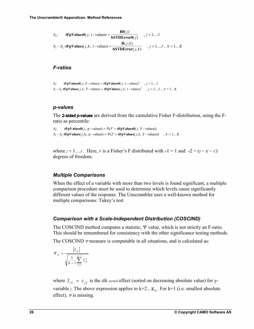
p-values
The 2222----sided psided psided psided p----valuesvaluesvaluesvalues are derived from the cumulative Fisher F-distribution, using the F-
ratio as percentile:
b j F j
b b j F j k k Kk
0
1 1
: ( , ) ( ( , ))
: ( , , ) ( ( , , ))
tFpValues0 tFpValues0
tFpValues tFpValues
p - values P F - values
k p - values P F - values ,
= >
− = > = K
where j = 1…J . Here, F is a Fisher’s F distributed with ν1 = 1 and ν2 = (I − K − C) degrees of freedom.
Multiple Comparisons
When the effect of a variable with more than two levels is found significant, a multiple
comparison procedure must be used to determine which levels cause significantly
different values of the response. The Unscrambler uses a well-known method for
multiple comparisons: Tukey’s test.
Comparison with a Scale-Independent Distribution (COSCIND)
The COSCIND method computes a statistic, Ψ value, which is not strictly an F-ratio.
This should be remembered for consistency with the other significance testing methods.
The COSCIND Ψ measure is computable in all situations, and is calculated as:
Ψ jk
jk
jn
n
k
z
kz
=
− =
−
∑
~
~1
1
2
1
1
where ~ ~z zj k j k= is the kth sorted effect (sorted on decreasing absolute value) for y-
variable j. The above expression applies to k=2...KE. For k=1 (i.e. smallest absolute
effect), Ψ is missing.

The Unscrambler® Appendices: Method References
© Copyright CAMO Software AS 27
The approximated p-values are calculated by Cochran’s approximation:
pValEff ( , , ) betai , ,, ...
j k kk
k
j J
k K
jk
COSCIND ,
= ⋅ −−
+−
=
=1
1
2
1
2
1
11
1
12Ψ
K
Here, betai(α, β, x) is the incomplete beta function.
Higher Order Interaction Effects (HOIE)
The F-ratio is found by:
FValEffX X
( , , )( )
,( )
j k Fb
Sj J k Kjk
jk
kk
E HOIE , HOIE, j
2
S
T
S
= =⋅
= =−
2
11 1K K
where
SI K C
f j JjB E
ij
i
HOIE
2
Cubesamples
, ,
{}
=− −
=∈∑1
12K
Leverage Calculations
The leverage of an object, a sample or a variable, describes its influential X-
“uniqueness” or its actual contribution to the calibration model. A leverage close to zero
indicates that the corresponding sample or variable had very little importance for the
calibration model.
For MLR, sample leverages are computed according to the following equation:
( )hI
i IiC
i i C= +−1
11
x X X xST
ST
S S , =, , K
For projection methods, sample and variable leverages are computed according to the
following equations:
Sample leverages are stored in the Hi matrix.
H1
I
t
t ti
ia
2
a
T
aa 1
A
= +=∑
Leverages of X-variables are stored in the Hk matrix.

The Unscrambler® Appendices: Method References
28 © Copyright CAMO Software AS
Hw
w wk
ik
2
a
T
aa 1
A
==∑
The validation method Leverage CorrectionLeverage CorrectionLeverage CorrectionLeverage Correction uses the leverages to estimate the prediction
error without actually performing any predictions. The correction is done by correcting
the y-residuals f with the sample leverage hi:
ff
1 hij
corrected ij
i
=−
Thus, the higher the leverage hi, the larger 1/(1-hi), and extreme samples will have
larger prediction residuals than average ones. This is a way to take into account the
influence these samples may have on the model.
High Leverage and Outlier Detection
Outlying samples or variables and unusually high leverages are detected in all analyses.
The tests listed in the table below are calculated where they are appropriate:

The Unscrambler® Appendices: Method References
© Copyright CAMO Software AS 29
Tests for leverage and outlier detection
Tests Equation
Leverage limit Hi( , )a i ha
C> 1
Ratio of Calibrated to Validated multiple correlation MultCorrCal
MultCorrVal
( , )
( , )
a j
a jC> 3
Statistical condition number limit γ > C4
Ratio of Calibrated to Validated explained variance ExpXCalTot
ExpXValTot
( )
( )
a
aC< 5
Total explained variance ExpXCalTot(a) < C6
Ratio of Validated to Calibrated multiple correlation MultCorrVal
MultCorrCal
( , )
( , )
a j
a jC> 7
Sample Outlier limit, Calibration Eix
ResXCalVar
( , , )
( , )
i k a
a kC> 8
Sample Outlier limit, Validation Eix
ResXValVar
( , , )
( , )
i k a
a kC> 9
Variable Outlier limit, Calibration ResYCalVar
ResYCalTot
( , )
( )
a j
aC> 10
Variable Outlier limit, Validation ResYValVar
ResYValTot
( , )
( )
a j
aC> 11
Ratio of Validated to Calibrated explained variance ExpXValTot
ExpXCalTot
( )
( )
a
aC< 12
Exchange X and Y in the matrices above according to the context in which the leverage
and outlier detection is done.
The constants “C” that are used as test limits are set in the Warning Limits dialog available
in all model dialogs from the Task menu. A warning is given when the calculated value
is higher/lower than the limit.
All issued warnings are found in the Outlier List.
Warning Limits and Outlier Warnings
The warning limits in The Unscrambler are listed in the table hereafter. In principle,
more than one limit may be applied for each test formula to distinguish between degrees
of severity, eg. “badly described” vs. “very badly described”. However, only one
constant is used to keep things as simple as possible.

The Unscrambler® Appendices: Method References
30 © Copyright CAMO Software AS
Constants in The Unscrambler
Constant Default value
Allowed
range
Comment
C1 3.0 2 − 10 Leverage limit
C2 6% 0% − 15% Residual variance increase limit
C3 2.0 1.5 − 5.0 Ratio of Calibrated to Validated multiple correlation
C4 50 10 − 1000 Statistical condition number limit
C5 0.5 0.2 − 0.7 Ratio of Calibrated to Validated residual variance
C6 20% 5% − 90% Total explained variance
C7 1.3 1.0 − 3.0 Ratio of Validated to Calibrated multiple correlation
C8 3.0 2 − 10 Sample Outlier limit, Calibration
C9 2.6 2 − 10 Sample Outlier limit, Validation
C10 3.0 2 − 10 Variable Outlier limit, Calibration
C11 3.0 2 − 10 Variable Outlier limit, Validation
C12 0.75 0.5 − 1.0 Ratio of Validated to Calibrated residual variance
C13 3.0 2 - 10 Individual Value Outlier, Calibration
C14 2.6 2 - 10 Individual Value Outlier, Validation
The table below shows which object warning each warning limit is used in. It also shows
upon which samples (cal/val) and variables the test is based. The sequence is as shown
in the user dialog for Warning Limits (PLS1).
Object warnings and warning limits
Constant Cal. Samples
Val. Samples
X Y Object Warnings (OW)
C1 X X 100,102
C8 X X X 121,123,102
C9 X X X 122,124
C13 X X X 130,140
C14 X X X 131,141
C10 X X X 150,160
C11 X X X 151,161
C6 X X X X 152,153,162,163
C5 X X 170,171
C12 X X 172,173
C2 X X X 180,181
C3 190
C4 200,201,202,205
C7 191

The Unscrambler® Appendices: Method References
© Copyright CAMO Software AS 31
The next table shows which warning limit is used in connection with which analysis.
Warning limits and analyses
Const. STA PCA PCR PLS MLR AoE RS PRE CLA
C1 � � � � �
C2 � � �
C3 �
C4 � �
C5 � � � �
C6 � � � �
C7 �
C8 � � � � � �
C9 � � � � �
C10 � � � � � �
C11 � � � �
C12 � � � �
C13 � � � � � �
C14 � � � � �
Hotelling T2 Computations
The Hotelling statistic is a multivariate t-statistic, and for an object i, it is given by
Var ta$ ( )
where Var ta$ ( ) is the estimated variance of ta. There is a relationship between T2 and the
F-statistic given by the expression
F T I I A A Ii≈ − −2 2 1* ( ) / ( )
which is F distributed with A and I-A degrees of freedom
I = Total number of observations in the model training set
A = Used number of components in the model
Then, for an observation i, this observation is outside the critical limit if
T A I I I A Fi critical
2 2 1> − − ⋅( ) / ( ) ,α

The Unscrambler® Appendices: Method References
32 © Copyright CAMO Software AS
The α value is commonly set to 0.05. The confidence region for a two-dimensional score
plot is an ellipse with axis
( $ ( ) ( ) / ( ( ))), ,
.Var t F I I Ia I⋅ ⋅ − −−2 2
2 0 52 1 2α
where a is [1 2] for the (1,2) score plot.
The T2 statistic for each sample and each PC, together with the critical limits are stored
in the result file.
Deviation in Prediction
The Unscrambler gives you an estimate of how reliable the predicted values are. This
estimate is calculated as
yD eviation = ResYValV arR esXValSamp
ResXValTotH i +
1
I
a 1
I
pred
cal cal
+
−
+
1
Note: The deviation calculated here is based on an approximation of the theoretical
variance of predictions under certain assumptions. It has recently been improved from a
previous formula (implemented in earlier versions of The Unscrambler) to make it more
robust.
You will find a detailed reference about this equation in De Vries and Ter Braak,
“Prediction Error in Partial Least Squares Regression: A Critique on the Deviation used
in The Unscrambler”, see Bibliographical References for details.
Classification Statistics
Various statistics are calculated in SIMCA classification to distinguish between
members and non-members of the different classes.
Sample to Model Distance
The distance from sample i to the model m is calculated as the orthogonal distance from
the sample down to the different classes defined by their principal components.

The Unscrambler® Appendices: Method References
© Copyright CAMO Software AS 33
New Samples
The distance of new samples to the class model m is computed as
S (m,i) ResXCal ( , i)i new,m= a
Calibration Samples
The distance of calibration samples from model q projected onto model m is computed
as
( )S (m, i)1
dEix i, ki
7q,m
2
= ∑
The distance of each sample i in model q to the class m is computed as
ModelDist (m, i) d ResXCal (a, i)q q,m= ⋅
where
( )
[ ]q m: d
d
d
K a I
I K CK amax I C, K
q m : d 1
7
6
q
q q
= = =−
− − −
≠ =
Model Distance
The model distance is the distance between pairs of classes in the classification. The
distance between two models, q and m, is calculated as follows:
( ) ( )
( ) ( )ModelDistance(q,m)
1
KS m,k
1
KS q,k
1
KS m,k
1
KS q, k
q
q
2
mk 1
Kq
m
2
k 1
Km
m
m
2
q
q
2
k 1
Kq
k 1
Km=
+
+
= =
==
∑ ∑
∑∑
where
( )S m kq , is the standard deviation for variable k when fitting samples from model q onto
model m, as an example.
( ) ( )
( ) ( )
q m: S m, k ResXCal a, k
q m: S m, k1
dEix i, k
q
2
q
2
3
2
i 1
I
= =
≠ ==∑
Discrimination Power
The discrimination power expresses how well a variable discriminates between different
classes. The discrimination power for variable k between model q and m (fitting samples
from model q onto model m) is computed as

The Unscrambler® Appendices: Method References
34 © Copyright CAMO Software AS
( ) ( )( ) ( )
DiscrPowerS m, k S m, k
S m, k S q, k
q
2
m
2
m
2
q
2=
+
+
Modeling Power
The modeling power describes the relevance of variable for one class. The modeling
power for variable k in model m is computed as
( )( )
ModelPower 1ResXCalVar a, k
ResXCalVar 0, k= −
Class Membership Limits
Two limits are used to decide whether a sample belongs to a certain class or not.
Leverage Limit
New samples are found to be within the leverage limits for a class model if
cI
a 13 HiClass(m)
+⋅≤
Sample to Model Distance Limit, Smax
The sample to model distance limit Smax for classifying new samples is calculated
differently depending on the validation method used for the class model m:
Leverage correction: ),1(F(m)S (m)S crit0max CAI −−=
Cross validation: ),1(F(m)S (m)S crit0max calI=
Test set: ),1(F(m)S (m)S crit0max TestI=
Where S0 is the average distance within the model:
( ) ( )S m ResXValTot a0 =
and C = 1 for centered models,
0 otherwise

The Unscrambler® Appendices: Method References
© Copyright CAMO Software AS 35
Computation of Transformations This chapter contains the formulas for most transformations implemented in The
Unscrambler. For some simple transformations (e.g. Average) not listed here, lookup the
corresponding menu option (e.g. Modify - Transform - Reduce (Average)) using the Index
tab in the Unscrambler Help System.
Smoothing Methods
The Unscrambler offers two kinds of smoothing; Moving Average and Savitzky-Golay
smoothing.
Moving Average Smoothing
For each point of the curve, a moving average is computed as the average over a
segment encompassing the current point. The individual values are replaced by the
corresponding moving averages.
Savitzky-Golay Smoothing
The Savitzky-Golay algorithm fits a polynomial to each successive curve segment, thus
replacing the original values with more regular variations. You can choose the length of
the segment (right and left of each point) and the order of the polynomial. Note that a
first-order polynomial is equivalent to a moving average.
The complete algorithm for Savitzky-Golay smoothing can be found in Press,
Tewkolsky, Vetterling and Flannery (see Bibliographical References for details).
Normalization Equations
The Unscrambler contains three normalization methods: mean, maximum, and range
normalization.
Mean Normalization
( ) ( )( )
X i , kX i , k
X i ,=
•
Maximum Normalization
( ) ( )( )( )
X i, kX i, k
max X i,=
•

The Unscrambler® Appendices: Method References
36 © Copyright CAMO Software AS
Range Normalization
( ) ( )( ) ( )
X i, kX i, k
max i, min i,=
• − •
Spectroscopic Transformation Equations
Transformations often needed for spectra are given here.
Reflectance to Absorbance Transformation
We assume that the instrument readings R (Reflectance) or T (Transmittance) are
expressed in fractions between 0 and 1. The readings may then be transformed to
apparent Absorbance (Optical Density) according to this equation.
M i kM i k
new( , ) log(( , )
)=1
Absorbance to Reflectance Transformation
An absorbance spectrum may be transformed to Reflectance/ Transmittance according to
this equation.
M i knewM i k( , ) ( , )= −10
Reflectance to Kubelka-Munk Transformation
A reflectance spectrum may be transformed into Kubelka-Munk units according to this
equation.
M i kM i k
M i knew ( , )
( ( , ))
( , )=
−⋅
1
2
2
Multiplicative Scatter Correction Equations
Multiplicative Scatter Correction (MSC) is a specific transformation for spectra. It
consists in fitting a separate regression line to each sample spectrum, expressed as a
function of the average value for each wavelength; the a and b coefficients of that
regression line are then used to correct the values of each sample.
Full MSC:
M i kM i k a
bnew ( , )( , )
=−
Common Offset: M i k M i k anew ( , ) ( , )= −

The Unscrambler® Appendices: Method References
© Copyright CAMO Software AS 37
Common Amplification:
M i kM i k
bnew ( , )( , )
=
Added Noise Equations
Proportional and additive noise can be added to selected variables. Proportional noise is
typically noise that affects the instrumental amplification. Additive noise is typically
noise that affects the measurement signal.
The formula for adding noise is
M i k M i kPN
N N ANnew ( , ) ( , ) , ) ( , )= ⋅ + ⋅
+1
1000 1 0
where
PN = Level of proportional noise in % AN = Level of additive noise N(m,s) = randomly distributed value with m = mean and s = standard deviation.
The amount of additive noise (AN) depends on the level of the measurement value. You
may calculate this value by
ANP
M i k= ⋅%
( , )100
where
P% is the level of approximate additive noise in percent.
Differentiation Algorithm
The differentiation of a curve (i.e. computing derivatives of the underlying function)
requires that the curve is continuous (no missing values are allowed in the Variable Set
that is to be differentiated).
Savitzky-Golay Differentiation
The Savitzky-Golay algorithm fits a polynomial to each successive curve segment, thus
replacing the original values with more regular variations. You can choose the length of
the segment (right and left of each point) and the order of the polynomial. Note that a
first-order polynomial is equivalent to a moving average.
The complete algorithm for Savitzky-Golay differentiation can be found in Press,
Tewkolsky, Vetterling and Flannery (see Bibliographical References for details).

The Unscrambler® Appendices: Method References
38 © Copyright CAMO Software AS
Mixture and D-Optimal Designs This chapter addresses the case of non-orthogonal designs, for which the shape of the
experimental region is essential in determining which points to include in the design.
Shape of the Mixture Region
The combinations of levels of mixture variables are always located on a simplex.
Depending on the nature of the ranges of variations and additional multi-linear
constraints, the mixture region may either be a simplex, or have a more complex shape.
Notations
The notations below are used in this section to express formulas and algorithms.
Notations for mixtures
Symbol
Description
q, Q Mixture variable no. and no. of mixture variables
U Upper bound of a variable
L Lower bound of a variable
MixSum Mixture sum of the mixture variables
Simplex Region
If the following criterion is true and there are no multi-linear constraints, then the
mixture region is a simplex:
For every U q
MixSum U Lq ii q
− ≤≠∑
Upper/Lower Bound Consistency
The mixture region is said to be inconsistent if any of the variables’ upper or lower
bounds are unattainable because of other variables constraints. If an inconsistent mixture
region is non-empty, it can be made consistent by lowering inconsistent upper bounds
and raising inconsistent lower bounds until they touch the region border.

The Unscrambler® Appendices: Method References
© Copyright CAMO Software AS 39
The region is non-empty if
U MixSumq∑ > and L MixSumq∑ <
If the region is empty by the first criteria, the user is asked to raise the upper constraints
of some of variables. If the region is empty by the second criteria, the user must lower
the lower constraints of some variables.
Multi-linear constraints are checked for consistency by running the CONVRT algorithm
to generate extreme vertex points. If there are inconsistent constraints, the algorithm will
return an error code.
Computation of Candidate Points for a D-Optimal Design
Generating candidate points for D-optimal design is based on the algorithms CONVRT
and CONAEV (CORNELL, 1990).
The CONVRT algorithm determines the extreme vertices mixture regions with linear
constraints. The CONAEV algorithm calculates the centroids of all N-dimensional
surfaces of the region, where 0<N<Q. The centroid points are calculated as the average
(mean) of the extreme vertices on the design region surface associated with the centroid
point.
D-Optimal Selection of Design Points
The D-optimal selection of a design point is based on the algorithm DOPT (MILLER
and NGUYEN, 1994).
The FORTRAN algorithm DOPT is used to D-optimally select a number of design
points from a set of candidate points. The design points are chosen so that the
determinant of X'X is maximized (X is the design point matrix).
DOPT:
6. Start with a default set of design points, or else generate a random set.
7. Calculate X'X for the selected points.

The Unscrambler® Appendices: Method References
40 © Copyright CAMO Software AS
8. As long as there is improvement do:
a. Find the selected point and unselected candidate point
which will improve the X'X determinant the most.
b. Exchange the points, and calculate new X'X.
Bibliographical References This chapter contains bibliographical references for the methods and algorithms used in
The Unscrambler.
About Statistics and Multivariate Data Analysis
• Albano C, Dunn III W, Edlund U, Johansson E, Nordén B,
Sjöström M, Wold S, Four levels of pattern recognition,
Anal. Chim. Acta, 1978, 103, 429 - 443
• Beebe KR, Kowalski BR, An introduction to multivariate
calibration and analysis, Anal. Chem., 1987, 57(17) 1007A - 1017A
• Box GEP, Hunter WG, Hunter JS, “Statistics for
experimenters”, Wiley & Sons Ltd, New York, 1978
• Brown SD, Blank TB, Sum ST, Weyer LG, Chemometrics,
Anal. Chem., 1994, 66, 315R - 359R
• De Vries S, Ter Braak Cajo JF, Prediction error in partial
least squares regression: a critique on the deviation used in
The Unscrambler, Chemometrics and Intelligent
Laboratory Systems, 1993, 30, 239 - 245
• Deming SN, Palasota JA, Nocerino JM, The geometry of
multivariate object preprocessing, Jour. Chemometrics,
1993, 7, 393 - 425
• Draper NR, Smith H, “Applied regression analysis”, John
Wiley & Sons, Inc, New York, 1981
• Esbensen K, “Multivariate Data Analysis - In Practice”,
ISBN 82-993330-3-2, CAMO Process AS, Oslo, 5th
Edition 2002
• Fisher RA, The use of multiple measurements in
taxonomic problems, Ann. Eugenics, 1936, 7, 179 - 188
• Forina M, Drava G, Boggia R, Lanteri S, Conti P,
Validation procedures in near-infrared spectrometry, Anal.
Chim. Acta, 1994, 295, 1-2, 109 - 118
• Frank IE, Friedman JH, A statistical view of some
chemometrics tools, Technometrics, 1993, 35, 109 - 148

The Unscrambler® Appendices: Method References
© Copyright CAMO Software AS 41
• Geladi P, Kowalski BR, Partial least-squares regression: a
tutorial, Anal. Chim. Acta, 1986, 185, 1 - 17
• Golub GH, Loan CF van, “Matrix Computation”, The John
Hopkins University Press, London, 1989, 2nd ed
• Höskuldsson A, PLS regression methods, Jour.
Chemometrics., 1988, 2, 211 - 228
• Jackson JE, “A User’s Guide to Principal Components”,
Wiley & Sons Inc., New York, 1991
• Johnson RA, Wichern DW, “Applied multivariate
statistical analysis”, 1988, Prentice-Hall, 607 p
• Manne R, Analysis of two partial least squares algorithms
for multivariate calibration, Chemom. Intell. Lab. Syst.,
1987, 2, 187 - 197
• Mardia KV, Kent JT, Bibby JM, “Multivariate Analysis”,
Academic Press Inc, London, 1979
• Martens H, Næs T, “Multivariate Calibration”, John Wiley
& Sons, Inc, Chichester, 1989
• Massart PL, Vandegiste BGM, Deming SN, Michotte Y,
Kaufman L, “Chemometrics: A text book”, Elsevier Publ.,
Amsterdam, 1988
• Wold S, Cross-validatory estimation of the number of
components in factor and principal components models,
Technometrics, 1978, 20(4), 397 - 405
• Wold S, Esbensen K, Geladi P, Principal component
analysis - A tutorial, Chemom. Intell. Lab. Syst., 1987, 2, 37 - 52
• Wold S, Pattern recognition by means of disjoint principal
components models, Pattern recognition, 1976, 8, 127 - 139
About Martens’ Uncertainty Test
• EFRON B., - 1982 -, The Jackknife, the Bootstrap and Other Resampling Plans, Society for Industrial and
Applied Mathematics, Philadelphia, Pennsylvania, ISBN 0-
89871-179-7
• MARTENS H., MARTENS M., - 1999 -, Modified Jack-
knife Estimation of Parameter Uncertainty in Bilinear
Modelling (PLSR), Food Quality and Preference.
• MARTENS H,. MARTENS M., - 1999 -, Validation of PLS Regression models in sensory science by extended

The Unscrambler® Appendices: Method References
42 © Copyright CAMO Software AS
cross-validation), PLS’99 (Proceedings, International
Symposium on PLS Methods, Paris Oct. 5-6, 1999.
• WESTAD F., BYSTRÖM M., MARTENS H., - 1999 -, Modified Jack-knifing in multivariate regression for
variable selection and model stability, NIR-99
(Proceedings, International Symposium on NIR
Spectroscopy, Verona June 13-18, 1999.
• WESTAD F., - 1999 -, Relevance and Parsimony in
Multivariate Modelling, Ph.D. Thesis, University NTNU
Trondheim, Trondheim, Norway.
About Three-way Data and Tri-PLS
• Bro R., “Multiway calibration. Multilinear PLS”, in
Journal of Chemometrics 10 (1):47-61, 1996
• Bro R., - 1998 -, Multi-way analysis in the food industry.
Models, algorithms and applications - PhD thesis,
University of Amsterdam, Netherlands
• Bro R., Smilde A. K. and de Jong S., “On the difference
between low-rank and subspace approximation: improved
model for multi-linear PLS regression”, in Chemom. Intell.
Lab. Syst. 58 (1):3-13, 2001
• Bro R. and Smilde A. K., “Centering and scaling in
component analysis”, in Journal of Chemometrics 17:16-
33, 2003
• Kiers H. A. L., “Towards a standardized notation and
terminology in multiway analysis”, in Journal of
Chemometrics 14 (3):105-122, 2000
• Sanchez E. and Kowalski B. R., “Tensorial calibration: I.
first-order calibration”, in Journal of Chemometrics 2:247-
263, 1988
About Experimental Design
• Box GEP, Hunter WG, Hunter JS, “Statistics for
experimenters”, Wiley & Sons Ltd, New York, 1978
• Carlson R, “Design and optimization in organic synthesis”,
Elsevier, Amsterdam, 1992
• Cornell J. A., - 1990 -, Experiments with Mixtures, John
Wiley & Sons, Inc., 2nd ed., 632p.
• Esbensen K, “Multivariate Data Analysis - In Practice”,
ISBN 82-993330-3-2, CAMO Process AS, Oslo, 5th
Edition 2002
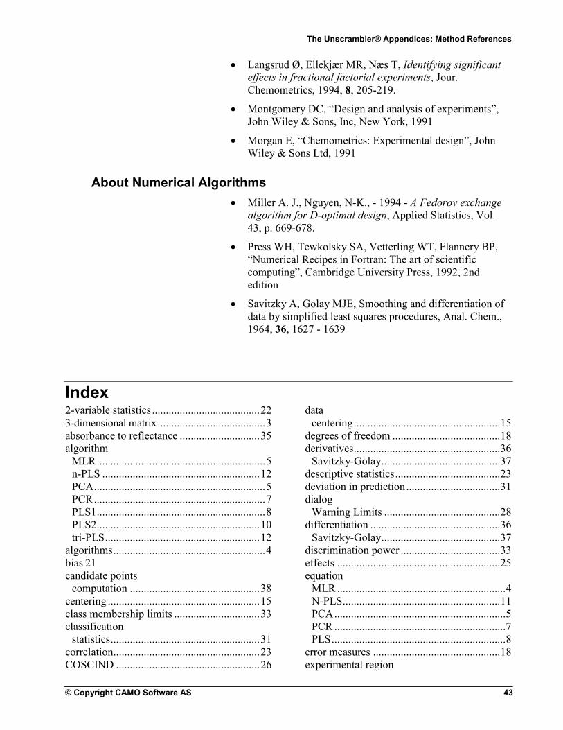
The Unscrambler® Appendices: Method References
© Copyright CAMO Software AS 43
• Langsrud Ø, Ellekjær MR, Næs T, Identifying significant
effects in fractional factorial experiments, Jour.
Chemometrics, 1994, 8, 205-219.
• Montgomery DC, “Design and analysis of experiments”,
John Wiley & Sons, Inc, New York, 1991
• Morgan E, “Chemometrics: Experimental design”, John
Wiley & Sons Ltd, 1991
About Numerical Algorithms
• Miller A. J., Nguyen, N-K., - 1994 - A Fedorov exchange
algorithm for D-optimal design, Applied Statistics, Vol.
43, p. 669-678.
• Press WH, Tewkolsky SA, Vetterling WT, Flannery BP,
“Numerical Recipes in Fortran: The art of scientific
computing”, Cambridge University Press, 1992, 2nd
edition
• Savitzky A, Golay MJE, Smoothing and differentiation of
data by simplified least squares procedures, Anal. Chem.,
1964, 36, 1627 - 1639
Index 2-variable statistics ....................................... 22
3-dimensional matrix ....................................... 3
absorbance to reflectance ............................. 35
algorithm
MLR ............................................................. 5
n-PLS ......................................................... 12
PCA .............................................................. 5
PCR .............................................................. 7
PLS1 ............................................................. 8
PLS2 ........................................................... 10
tri-PLS ........................................................ 12
algorithms ....................................................... 4
bias 21
candidate points
computation ............................................... 38
centering ....................................................... 15
class membership limits ............................... 33
classification
statistics ...................................................... 31
correlation ..................................................... 23
COSCIND .................................................... 26
data
centering ..................................................... 15
degrees of freedom ....................................... 18
derivatives ..................................................... 36
Savitzky-Golay ........................................... 37
descriptive statistics ...................................... 23
deviation in prediction .................................. 31
dialog
Warning Limits .......................................... 28
differentiation ............................................... 36
Savitzky-Golay ........................................... 37
discrimination power .................................... 33
effects ........................................................... 25
equation
MLR ............................................................. 4
N-PLS ......................................................... 11
PCA .............................................................. 5
PCR .............................................................. 7
PLS ............................................................... 8
error measures .............................................. 18
experimental region

The Unscrambler® Appendices: Method References
44 © Copyright CAMO Software AS
shape for mixtures ...................................... 37
explained variance ........................................ 20
f-ratio ............................................................ 25
higher order interaction effects .................... 26
histogram
statistics ...................................................... 23
HOIE ............................................................ 26
Hotelling T2 ................................................. 30
interaction and square effects ....................... 16
interaction effects ......................................... 16
interactions ................................................... 16
Kubelka-Munk ............................................. 35
kurtosis ......................................................... 24
leverage .................................................. 27; 28
lower bound .................................................. 38
maximum normalization .............................. 35
mean normalization ...................................... 35
MLR
algorithm ...................................................... 5
equation ........................................................ 4
model
equations ...................................................... 4
model distance .............................................. 32
modeling power ............................................ 33
moving average ............................................ 34
MSC ............................................................. 36
multiple comparisons ................................... 26
multiplicative scatter correction ................... 36
NIPALS algorithm ......................................... 6
noise
added .......................................................... 36
normalization ................................................ 34
n-PLS
algorithm .................................................... 12
N-PLS
equation ...................................................... 11
outlier
list ............................................................... 28
outlier detection ............................................ 28
outlier warnings ............................................ 29
OW 29
PCA
algorithm ...................................................... 5
equation ........................................................ 5
PCR
algorithm ...................................................... 7
equation ........................................................ 7
percentiles ..................................................... 24
PLS
equation ........................................................ 8
PLS1
algorithm ...................................................... 8
PLS2
algorithm .................................................... 10
preliminary scores ............................................ 3
p-value .......................................................... 26
range normalization ...................................... 35
reflectance to absorbance ............................. 35
reflectance to Kubelka-Munk ....................... 35
regression
statistics ...................................................... 22
residual variance ........................................... 19
residuals ................................................. 18; 19
ResYCalSamp ............................................... 19
ResYValSamp .............................................. 19
RMSEC .................................................. 18; 21
RMSED ........................................................ 23
RMSEP .................................................. 18; 21
root mean square error .................................. 21
root mean squared error of deviation .......... See
RMSED
Savitzky-Golay ...................................... 34; 37
scalar ............................................................... 3
scores
preliminary .................................................... 3
SED ............................................................... 23
SEP 21
Si 32
significance testing ....................................... 25
SIMCA ......................................................... 31
simplex region .............................................. 37
singular value decomposition ......................... 5
skewness ....................................................... 24
smoothing ..................................................... 34
moving average .......................................... 34
Savitzky-Golay ........................................... 34
spectroscopic transformations ...................... 35
square effects ................................................ 16
standard
error of deviation ........................................ 23
error of prediction ...................................... 21
error of the B-coefficients .......................... 25
standard deviation ......................................... 23
studentized residuals ..................................... 22

The Unscrambler® Appendices: Method References
© Copyright CAMO Software AS 45
SVD ................................................................ 5
total residual variance ................................... 20
tri-PLS
algorithm .................................................... 12
t-values ......................................................... 25
upper bound .................................................. 38
variances ....................................................... 18
vector............................................................... 3
warning limits ............................................... 29
Warning Limits dialog .................................. 28