THE UNOBSERVED RETURNS FROM

ENTREPRENEURSHIP∗

Sarada†

Duke University

July 2013

Abstract

This paper resolves a longstanding empirical puzzle: that most entrepreneurs persist de-

spite lower initial earnings and earnings growth. I hypothesize that expenditure is a better

measure of self-employment returns than reported income, suffering from fewer biases. Us-

ing 38 years of longitudinal data, I find that while individuals report earning 26.2% less in

self-employment, their expenditures are 4.5% higher than in their observed alternative. This

increase comes from those who persist in self-employment, where expenditure is no different

upon initial entry but grows by 0.8% with each additional year of survival. Savings are also

higher for those who persist where wealth goes up by $25,000 with each additional year of sur-

vival. The combined findings of increased expenditure and savings that coincide with time in

self-employment indicate higher earnings for those who remain so. These gains do not appear

∗I am very grateful to Roger Gordon for the invaluable advice and guidance he has given me. I would alsolike to thank Prashant Bharadwaj, Steve Bond, Tiffany Chou, Wes Cohen, Julie Cullen, Scott Dyreng, Silke Forbes,Youjin Hahn, Campbell Harvey, Leora Klapper, Craig McIntosh, Karthik Muralidharan, Philip Neary, Paul Niehaus,Manju Puri, David Robinson, Therese Scharlemann, Oana Tocoian, Annette Vissing-Jorgensen, Christopher Woodruff,Nicolas Zeibarth, an anonymous referee, participants at the 2013 NBER SI, the Northwestern Searle Conference andseminar participants at UCSD, University of Iowa, Claremont McKenna College and Duke University for their helpfulcomments. Finally, I would like to thank the Kauffman Foundation for their generous support. The opinions andconclusions expressed in this paper, and all remaining errors are solely mine.†sarada.x@duke.edu; 100 Fuqua Drive, Durham, NC 27708; (919) 660 7964; http://people.duke.edu/∼sx19/

1

to be offset by higher uncertainty. In studying the consumption and wealth dynamics prior to

entry, I find that the switch into self-employment is not driven by sudden gains (or losses) in

wealth. This lends further credence to the use of changes in expenditure and wealth to proxy

for changes in self-employment earnings. The findings in this paper are consistent with stan-

dard occupational choice models and show that for those who make the choice, the decision

to remain self-employed can be rationalized using just financial motivations. Other findings

are that hours worked also grow with time in self-employment, and that post-self-employment,

labor market outcomes vary by skill level.

Keywords: Occupational choice; self-employment; entrepreneurship; consumption; savings

JEL Classification: E21, E24, E26, H26, J2

Total Word Count: 20,867 (including abstract, text, footnotes, appendix, references, tables

and figures)

2

1 Introduction

Entrepreneurial activity is a key generator of economic development. Individuals and firms in-

volved in such undertakings innovate on both the product and process margins, creating new tech-

nologies and organizational novelties. Entrepreneurs are willing to internalize the risk involved

in implementing new ideas, thereby bringing about positive externalities. The macroeconomic

returns to entrepreneurial activity are clear; entrepreneurs modernize, create employment, bring

about positive spillovers, and engender economic growth. However, these positive returns do not

translate quite so seamlessly at the microeconomic, individual level.

While standard occupational choice models (Jovanovic (1982), Roy (1951)) predict, that indi-

viduals will attach themselves to the employment type wherein their skills are best compensated,

empirical evidence seems to suggest otherwise. It is not clear that individuals engaging in en-

trepreneurial activity always yield higher, or even equivalent returns to what they could otherwise

receive in wage employment. Specifically, Hamilton (2000) finds that in her tenth year, the me-

dian self-employed individual makes 35 percent less than her wage-employed counterpart. This

finding gives rise to the question: what, if not financial returns, propels individuals to remain

self-employed?

The literature currently proposes a few explanations to rationalize the curious observation, that

individuals choose self-employment despite the low returns. These explanations can be broadly

categorized into heterogeneity in individual preferences over employment types, risk and time, and

differences in beliefs (Camerer and Lovallo, 1999; Cooper et al., 1988; Hamilton, 2000; Blanch-

flower et al., 2001; Moskowitz and Vissing-Jørgensen, 2002; Puri and Robinson, 2013). In other

words, rather than just maximizing wealth in the safest possible way, the self-employed may sim-

ply prefer working for themselves, have a higher risk tolerance or be over-optimistic.

In this paper, I employ data from the Panel Study of Income Dynamics (PSID) and show, with-

out alluding to any preference arguments, that this empirical puzzle can be explained by measuring

3

the returns to self-employment using household expenditure and savings, rather than reported earn-

ings. The findings are easily rationalized within standard occupational choice models of wealth

maximizing agents (Jovanovic (1982), Roy (1951)). Using 38 years of longitudinal data, I find that

while individuals report earning 26.2 percent less in self-employment than in wage-employment,

they in fact consume 4.5 percent more. This 4.5 percent expenditure increase comes from those

who persist in self-employment where expenditure upon initial entry is the same as before but

grows by 0.85 percent with each additional year survived. Individuals also save more in self-

employment with average wealth being $138,000 higher than in wage-employment. Once again,

persistence in self-employment is the driver of this finding with wealth being no different upon

initial entry, but increasing by $25,000 with each additional year. Since income can only be used

in two ways, to consume and to save, the combined findings of higher expenditure and savings

provides compelling evidence for increased earnings in self-employment.

The results above are derived by having changes in household expenditure surrogate for changes

in the true financial return from work, which for the self-employed, does not equal reported earn-

ings. Self-reported income is not a reliable measure of the financial returns to self-employment

for a variety of reasons, ranging from tax avoidance and the misclassification of income in survey

data, to failure in capturing expected future gains.1 Expenditure on the other hand, captures all

avenues of current financial gains and the permanent income hypothesis tells us that, so long as

future gains are anticipated and credit markets function, they should reflect in current expendi-

ture. Furthermore, unlike income, there is no incentive to systematically misreport expenditure for

survey purposes.

While this is not the first paper to use household expenditure in the study of self-employment

earnings (see Pissarides and Weber (1989) and Hurst et al. (2010)), my approach differs from

prior work. I estimate individual fixed effects over 38 years of longitudinal data, which allows

me to compare the expenditure and wealth patterns of the same individual in self-employment to

1Section 3 details four specific sources of this mis-measurement.

4

herself in other states. Thus, I do not rely on cross-sectional comparisons of reported income and

expenditure between wage and salary workers to infer self-employment earnings. Consequently,

I do not need to make assumptions about income elasticities. In fact, I largely do away with the

use of reported income, aside from showing that for the self-employed it is wildly inaccurate. This

approach allows me to answer, at least in part, what the financial returns from self-employment are

for those who make the switch, and in particular, persist. One obvious limitation to bear in mind

is that I only observe realized outcomes and cannot observe counterfactual earnings had one not

entered self-employment. Regardless, the results are striking and show that those who persist in

self-employment are financially better off than they were prior to entry.

In addition to the findings on increased expenditure and savings, the empirics also show that

individuals who move into self-employment do not experience significant increases in uncertainty,

in either expenditure or savings. Insofar as increased variance in expenditure and savings capture

volatility in business earnings, this finding indicates that the self-employed are not necessarily

trading off higher earnings with higher risk. In fact, the results in this paper confirm Moskowitz

and Vissing-Jørgensen (2002)’s finding that business owners highly concentrate their investments

within their own businesses. However, increased expenditure and savings at no observable cost in

realized uncertainty, suggests that the risk-return tradeoff may not be as difficult to rationalize as

previously thought.

This paper also finds, consistent with previous work (Hurst et al. (2010), Puri and Robinson

(2013)), that the self-employed work longer hours. What is especially interesting and up until

now undocumented, is the finding that this increase in work hours also accrues from time in self-

employment; upon entry, hours worked are about six percent lower, but with each additional year

of persistence grows by 1.15 percent. This suggests that with each additional year of survival,

one receives positive news about the viability of their business, which then induces more effort,

especially since the returns to effort are fully internalized by the entrepreneur.

While the results on expenditure, savings and uncertainty indicate that those who choose to

5

remain self-employed are financially better off, this increase in hours worked constrains the inter-

pretation that overall utility also goes up. However, given the previous literature on non-pecuniary

returns,2 one could argue that those who choose to persist in self-employment are better off, both

financially and non-financially.

Since the majority of those who try self-employment leave within 3 years, it is useful to look

at their economic outcomes, especially since this paper seeks to document the returns from self-

employment. The results show that post self-employment, low skilled workers suffer from worse

labor market outcomes, while high skilled workers appear to experience wage gains.This suggests

the presence of “necessity” and “opportunity” entrepreneurs, where the former group suffers from

weak labor market outcomes both in and out of self-employment, while the latter group enters

voluntarily and has the potential to reap subsequent wage gains from self-employment experience.

This paper is one of few (Evans and Leighton, 1989), to look at self-employment returns in

a long panel setting, which enables the tracking of individuals over time and across employment

spells. The three main contributions of the paper are that first, I propose a variety of avenues for

earnings amongst the self-employed that may evade reported income which enables me to define

the total financial return to self-employment. Second, I theoretically describe how this newly

defined total financial return maps to consumption and savings, and use these new measures to

estimate the financial returns from self-employment. Third, I exploit 38 years of longitudinal data

to study a variety of features relating to pre, during and post self-employment outcomes.

The rest of the paper is organized as follows. The next section goes over predictions from

two relevant occupational choice models. Section 3 documents the various avenues for financial

gains in self-employment, defines the total return to self-employment and then explains how this

return maps to changes in household expenditure and savings. Section 4 describes demographic,

employment and expenditure data from the PSID, and presents summary statistics. Section 5,

2More recent work by Hurst and Pugsley (2010) convincingly shows that business owners do in fact enjoy non-pecuniary benefits.

6

outlines my estimation strategies and discuss the empirical findings. Lastly, section 6 posits some

implications that arise from the empirical findings, and concludes.

2 Theoretical Predictions

In this section, I focus on two occupational choice models that describe the decision wealth max-

imizing individuals make when attaching themselves to a given occupation. The first model is a

“matching model” proposed in Roy (1951), and the second model is a “learning model” proposed

in Jovanovic (1982). While I will not formally develop the arguments in these two models, the

predictions from both are so intuitive that they can be summarized in a few sentences. In his 1951

work entitled, “Some Thoughts on the Distribution of Earnings,” Roy, without alluding to a single

equation, lucidly outlines an occupational choice model. Roy’s model predicts that when individ-

uals have unobserved time invariant, sector specific skills of which they are fully aware, they will

accordingly attach themselves to the sector wherein they have a comparative advantage. Thereby,

matching themselves to the employment type in which they will yield the highest financial return.3

Jovanovic’s model on the other hand begins from the premise that individuals have imperfect infor-

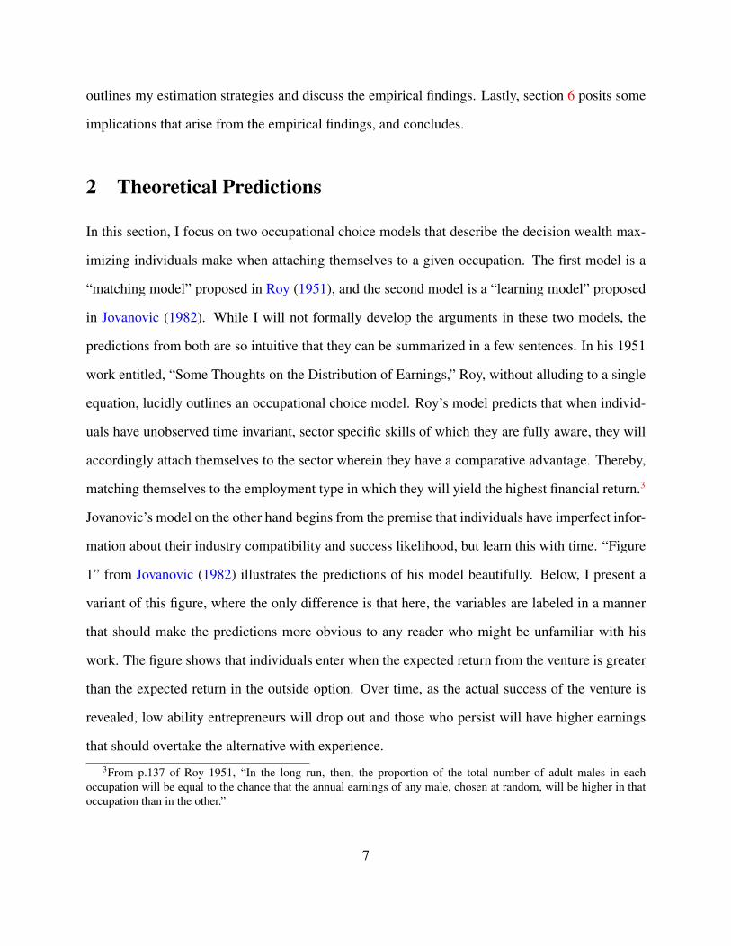
mation about their industry compatibility and success likelihood, but learn this with time. “Figure

1” from Jovanovic (1982) illustrates the predictions of his model beautifully. Below, I present a

variant of this figure, where the only difference is that here, the variables are labeled in a manner

that should make the predictions more obvious to any reader who might be unfamiliar with his

work. The figure shows that individuals enter when the expected return from the venture is greater

than the expected return in the outside option. Over time, as the actual success of the venture is

revealed, low ability entrepreneurs will drop out and those who persist will have higher earnings

that should overtake the alternative with experience.

3From p.137 of Roy 1951, “In the long run, then, the proportion of the total number of adult males in eachoccupation will be equal to the chance that the annual earnings of any male, chosen at random, will be higher in thatoccupation than in the other.”

7

“Figure 1” from Jovanovic (1982)

Simply put, these models imply that when individuals seek to maximize wealth, the empirical

researcher should observe that they are better off financially in the employment choice they vol-

untarily choose and persist in. In a longitudinal assessment of outcomes, we should observe that

over the long run, individuals will persist in the employment type wherein they have a comparative

advantage, resulting in higher financial gains as compared to that in the feasible alternative. How-

ever, as described in Jovanovic (1982), if individuals do not have perfect information about their

industry compatibility, but are able to learn over time, we should then see some individuals enter-

ing self-employment and then leaving once they learn where their skills are better compensated.4

Those remaining in self-employment should continue to be financially better off.

The empirical results presented in this paper are consistent with both these models. While in-

tuitive, this result is not not easily obtained. The key innovation in establishing this consistency

between the theories described here and the empirics, is my use of fixed effects estimations and

of changes in household expenditures and wealth, rather than reported earnings. In the next sec-

4For the truly low skilled, this may even mean returning to unemployment or employment with very low returnssince these might be the only options available to them. It is important to bear in mind that there will be empiricaldifferences in post-self-employment outcomes for those who enter voluntarily (i.e. those who have competitive outsideoptions) versus those who enter involuntarily.

8

tion, I will go into detail on what the financial returns to self-employment are, and how income

maps to expenditure and savings, which I then argue are superior measures of the returns to self-

employment.

3 The total financial return to self-employment, and expendi-

ture as its measure

In this section, I detail reasons for why household expenditure is a more accurate representation of

the returns to self-employment, than reported earnings. Before I delve into this discussion, I will

first document the avenues for compensation in self-employment that may evade reported earnings

(section 3.1), and then explain how these avenues can manifest in expenditures. The remainder of

this section will describe how expenditure maps to income, thereby warranting its use as a proxy

for earnings in the empirical estimations.

Self-employed individuals are financially compensated in multiple ways. Some of these are

easily observed while others are less obvious, and yet others are totally unobserved in any report

of earnings, be they personal or business. Reported personal and business income are the easily

observed components of self-employment earnings. However, unlike most wage employees, the

self-employed have in addition, a variety of ways to compensate themselves. Here I will discuss the

four main avenues for additional compensation. These four avenues include: tax evasion, different

forms of income, reclassification of employment, and human capital accumulation. Tax evasion is

simply the phenomenon of understating income to avoid tax payments, while the use of different

forms of income is more subtle yet still unlikely to appear as self-employment earnings in survey

data. Reclassification of employment occurs when exceptional entrepreneurs get bought-out or

fully incorporate, thereby reclassifying as wage-employed (or retired), prior to receiving the bulk

of their payout. Human capital accumulation refers to the possibility of gaining skills, even from

failed entrepreneurial ventures, that may result in increases in productivity and earnings in post

9

self-employment wage work. These four thus far unobserved (or at least, less well measured) av-

enues for financial returns to self-employment render reported earnings a less effectual measure of

the true monetary returns to entrepreneurship. Each of these four components is more thoroughly

described below, and section 3.3 expounds on how using expenditure captures these additional

avenues for gains that elude reported income.

3.1 Four additional avenues for compensation

3.1.1 Tax evasion

That the self-employed understate income and overstate expenditures has been widely acknowl-

edged in both the tax enforcement and self-employment literatures. As documented in Andreoni et

al. (1998) and Slemrod (2007), reported income is not a good measure of the true financial returns

to self-employment due to the different avenues for reporting, or lack thereof, available to the self-

employed but not the wage employed. The self-employed have a greater degree of discretion than

the wage employed in where and whether to report income and expenses. So long as tax rates on

earnings are positive, business owners have an incentive to underreport their business income. An-

dreoni et al. (1998) find that taxpayers who have derived income from farms or sole proprietorships

tend to understate their taxes by considerably more than other taxpayers. They find, using 1985

US data, that sole-proprietors are likely to understate taxes between between 16 and 39 percent,

depending on occupation. More recent evidence from Slemrod (2007) corroborates this finding.

Slemrod reports that wage income is underreported by 1 percent, while business income is under-

reported by between 18 and 57 percent,5 depending on the business classification, with non-farm

proprietor income having both the largest tax gap and the highest rate of underreporting.

The study of tax evasion as it relates to returns in self-employment long predates the current

wave of papers on self-employment, and was first formally studied in this specific context by Pis-

5Excluding farm businesses.

10

sarides and Weber (1989). In their paper, the authors estimate the relationship between income

and consumption for the wage-employed, and use the coefficients obtained on income to predict

consumption for the self-employed. The difference between this predicted and observed consump-

tion is attributed to tax evasion amongst the self-employed. Using this methodology, the authors

conclude that on average, self-employment income in the UK is 1.55 times greater than that which

is reported. Using a similar strategy, but this time with US data, Hurst et al. (2010) find a 30

percent difference between predicted and actual consumption amongst the self-employed, which

they attribute to underreporting. While these two papers formally address the problem of tax eva-

sion, many papers, including both Hamilton (2000) and Moskowitz and Vissing-Jørgensen (2002),

acknowledge and attempt to account for this in their respective estimations.6

In this paper, I neither attempt to estimate the degree of tax evasion nor seek to attribute the

observed difference between income and expenditures solely to tax evasion. Instead, I propose

reasons, including but not exclusive to tax evasion, for why income is a weak measure and then

proceed to measure the returns to, and characterize the environment of, self-employment using

expenditures. It is my use of this new measure to rationalize the risk-return tradeoff being made

in the decision to persist in self-employment that, to the best of my knowledge, distinctly sets this

paper apart from other work in the literature.

3.1.2 Different forms of income and retained earnings

Another source of mis-measurement arises since the self-employed have the ability to pay them-

selves in different, less easily quantifiable forms. For example, the entrepreneur may choose to

retain her earnings within the business, especially if she learns that the venture has good prospects.

If the business is incorporated, the entrepreneur has the option of pumping liquidity back into the

6 Hamilton (2000) argues that one of the alternative measures he uses, “Equity Adjusted Earnings” is not reportedto tax authorities and may therefore suffer less from underreporting issues while Moskowitz and Vissing-Jørgensen(2002) add a 20 percent underreporting adjustment to total corporate profits in their estimations.

11

business and rather than draw a salary, compensate herself instead in firm shares.7 She can declare

a very low value for these firm shares on which she will pay current income tax. As the business

matures and she cashes these shares, she will only pay capital gains taxes (substantially lower than

income tax) on the appreciated value of those shares.8 Business owners may also receive income

through dividends, interest, annuities, rents and royalties. These various different forms of income

are also known as investment incomes and are not necessarily imputed into a business owner’s

salary income.

Note that the premise here is different from that of tax evasion. Having access to different

compensation mechanisms is independent of whether or not individuals deliberately underreport

earnings. In fact, much of the income discussed in this section is indeed reported on tax returns,

but not in a way that shows up as easily as self-employment income. If an individual cannot be

tracked for a long enough time and/or we cannot with confidence parse out the origin of their non-

wage income, as empirical researchers we may never fully observe and correctly classify these

additional avenues for financial gains. As such, most datasets, even long panel surveys like the

PSID, may not track individuals for a sufficiently large number of years so as to enable us to

qualify all financial gains from self-employment. Furthermore asset returns in this dataset are for

the most part agglomerated across all sources, be they business or personal. Since we may not

be able to confidently identify the provenance of the income source, it then becomes difficult to

consider these returns as business income. As a result, any reported income statistic we observe,

may be an underestimate.

7This example, where the entrepreneur can pay herself in firm shares, only relates to incorporated businesses. Inthe case of sole proprietorships and partnerships, earnings can be retained in the anticipation that they will yield ahigher return if reinvested in the business. When these returns are realized and cashed out by the business owner,everything is taxed as ordinary income so long as the business is not incorporated.

8Note that there are also special capital gains provisions for small businesses with capital gains taxed at half of thestandard rate, but capital losses treated as ordinary losses that become fully deductible up to a reasonably high limit.

12

3.1.3 Reclassification of employment type

A third source of mis-measurement emerges when firms that perform particularly well incorpo-

rate,9 get bought out, merge with other firms, or become publicly listed. When this happens,

the successful entrepreneurs who founded these firms may no longer appear in the data as self-

employed. Instead they take on job titles such as CEO or director, or become board members.

This results in them being reclassified as wage-employed or retired in the data after some time.

When evaluating the longer term returns to self-employment, this could lead to underestimation

since the most successful self-employed individuals are those who are most likely to be reclassi-

fied as wage-employees so as to ensure accountability to either shareholders or firm partners. Some

entrepreneurs may even choose to retire (or receive a “golden parachute” if bought out) upon re-

alizing high levels of success. Whether an individual is reclassified as wage-employed or retires

as a result of entrepreneurial success, the financial return they reap will be missed in the empirics,

especially if a lump sum payout occurs upon the sale or public listing of the firm at which point

these individuals no longer appear as self-employed in the data. While this may not impact the

vast majority of small businesses, the omitted financial returns may be sufficiently high such that

not accounting for this will unduly bias downward the returns to entrepreneurship.

3.1.4 Human Capital Accumulation

A fourth issue to consider is that the returns to self-employment may manifest beyond those periods

when an individual is self-employed. It is conceivable that individuals gain some skills when they

run their own business even if the venture eventually fails. Wage-workers are generally subject to

performing specific tasks while the self-employed, in order to run all aspects of their businesses

9From a survey perspective, it is unclear whether founders of incorporated firms will report themselves as employ-ees (CEO) or as self-employed. Ideally the returns to entrepreneurship (or being a business owner) should include allfirm founders, regardless of incorporation status. Since incorporated entities are usually the more successful ones, ifsome fraction of incorporated firm founders do not report themselves as being self-employed, the results in this paperare then most likely providing a lower bound for the true returns to entrepreneurship.

13

have to multi-task. Consider the following two scenarios. Scenario 1: Take an accountant working

for a wage at a firm who only needs to have expertise in the specific tasks she is required to perform.

When this same individual owns her own accounting business instead, she has to acquire (or is at

least exposed to) the various different managerial and organizational skills that are necessary to

run her business. Even if the business were to go bust, the individual is still in possession of the

multi-faceted skills she had picked up. As such, the wage-employee who attempts entrepreneurial

activity becomes a “jack-of-all-trades” (Lazear, 2004). Upon returning to wage-employment, these

new skills in addition to those she originally had, could cause her marginal productivity to be

different, presumably higher all else equal. Scenario 2: In this case individuals may already posses

multi-faceted capabilities and enter self-employment simply to signal to future employers that they

are able to or are at least familiar with managing a business which will hopefully alter their wage

path. This effect changes the true return to self-employment to a more lasting one that survives

beyond one’s tenure in self-employment. This argument is akin to that of investment in education

so as to boost future employment returns. If in fact this is the case, and ever having entered self-

employment influences future wage outcomes positively then one need not be much less risk averse

to justify entry into self-employment.10

3.2 Putting it all together: What are the financial returns to self-employment?

Given the avenues documented so far, what then are the financial returns to self-employment?

Below I specify the total financial return to self-employment for individual i at time t, denoted by

10This complementarity between self-employment and future returns in employment most likely holds for the highlyskilled, rather than unskilled workers. Anecdotally, tech companies in the likes of Silicon Valley see “failed” highskilled entrepreneurs as assets, while the “failed” self-employed gardener probably has less of a market value for hisself-employment experience. Owning a business signals different things to different employers. The results in thepaper suggest that high skilled individuals are more likely to either gain human capital or signal quality that is valuedby future employers, while low skilled individuals, if anything, perform much worse in post-self-employment wagework.

14

Rse,i,t.

Rse,i,t = Di,t + Ui,t + ∆Bi,t + E(HCwe,i,t) (1)

where Di,t is declared earnings, including reported salary/wage and reported investment earnings,

that are subject to income tax. Ui,t is undeclared earnings. This includes underreported earnings,

overstated business expenses and the value of personal consumption that is deducted as a busi-

ness expense. ∆Bi,t is the change in business value between between periods t − 1 and t, and

E(HCwe,i,t) is the annuity value of the expected gain (or loss) in future wage employment that is

attributed to the incremental experience in self-employment.

From this very simple equation, it is clear that most datasets surveying both personal and

business income will not capture the full financial return to self-employment accurately. Di,t can

be identified with some confidence, but for sole proprietors and partnerships, it is still difficult to

attribute the investment income components as returns from self-employment. Disposable income

then becomes even harder to pin down since to the empirical researcher using survey data, it isn’t

clear what tax rate an individual faces, even on just the declared portion of earnings. Needless

to say, Ui,t is completely omitted from any reported information. The IRS does provide some

estimates of underreporting, but the ranges are large (see section 3.1.1) and more importantly,

for any given individual, it is impossible to tell where in this range they may fall. ∆Bi,t is to

some extent observable in survey data. Various datasets, including PSID, SIPP and NSSBF11

amongst others, collect information on business value less business debt. The problem here is that

businesses are notoriously hard to value, especially in their nascent stages. The entrepreneur may

have private information on the viability of her business investments. Therefore simply looking

at the current reported market value, which is the number observed by the empirical researcher, is

not necessarily commensurate with the true present value of the business. Lastly, while HCwe,i,t is

11PSID: Panel Study of Income Dynamics, SIPP: Survey of Income and Program Participation, NSSBF: National-Survey of Small Business Finances

15

not observed for an individual when self-employed, the empirical researcher can attempt to parse

this out in longitudinal data. Evans and Leighton (1989) allude to this by showing that on average

self-employment experience is not associated with lower returns in future wage work. However,

skills acquired from self-employment that are compensated in future wage work have largely been

ignored as an avenue of financial returns within the literature.

While in this section, I have gone into significant detail on the various modes for financial

returns in self-employment, parsing them out in the empirics is beyond the scope of the paper.

Rather, the point of discussing them is to first, document the financial returns to self-employment

and second, to sketch the logic for why a new measure is necessary. The next subsection goes into

how expenditure captures more information on the financial state of the self-employed than any

other measure we currently have.

3.3 How does expenditure capture the financial returns to self-employment?

Ideally, the empirical researcher would like to observe each component of the financial returns to

self-employment from equation (1). However, this is not easily feasible, and even in the hypo-

thetical situation that it were, one would need to follow individuals for a long enough period of

time, in order to capture some of these returns that do not manifest immediately. I propose that

household expenditure, and in particular, the longitudinal dynamics of household expenditure, will

capture much more information on the financial returns to self-employment than any other measure

currently at our disposal.12

First, unlike that for reported income,13 there is no incentive for individuals to systemati-

cally misreport household expenditures (Meyer and Sullivan, 2003), particularly for survey pur-

12These other available measures include reported personal and business income from survey data, W-2 filings forself-employment earnings and tax filings for business income.

13It is reasonable to assume that methods used to underreport income for tax purposes will lead to an underreportingfor purposes of the survey, since maintaining consistency across tax filings and survey responses involves easier recalland avoids any perceived tax enforcement complications that the responded may be apprehensive of.

16

poses.14,15,16

Second, expenditures capture all the various avenues for both realized and anticipated financial

gains. I justify the use of expenditure as a reflection of current income since according to the per-

manent income hypothesis, current consumption (expenditure) is a reflection of contemporaneous

income and expected future income (Friedman, 1957; Hall, 1978). New information about future

income that arises during entry into self-employment shows up both as an unexpected change in

income and consumption. The change in consumption should theoretically equal some fraction of

the present value of the change in future income, and will be equal to the change in current income

only when this change is permanent. Therefore, measurement aside, income and consumption

measure the same thing, but in different ways.17 and the distinction between the two is based on

measurement per se.

Below I provide an informal sketch of how income maps to consumption in any given period

and then walk through how, and to what extent changes in consumption can be attributed to changes

in self-employment earnings. I will begin from the premise that consumption in any given period

is a function of income (both labor and non-labor), wealth and expectations about future earnings.

14The measure of expenditure used in this paper mainly comprises of food, rent and imputed rent. These basiccomponents of expenditure are especially unlikely to suffer for misreporting incentives, unlike large purchases suchas fine jewelry and luxury boats, which the respondent may deem as risky to report if they were in fact underreportingincome. See section 4.2 for a more detailed description of the expenditure measure.

15Issues of recall may be an issue, but so long as this isn’t a systematic problem amongst the self-employed in away that is different from that for the wage-employed, this is not of great concern.

16However, there still exists the possibility that expenditure for the self-employed may occur in part through businessexpenses. For example, transport charges, food consumed during work hours, conferences in resorts etc are notreported as personal expenses, but rather as business expenses. This then leads to an understatement of expenditure forthe self-employed. I partly address this issue in section 4.2, by looking at how budget shares of the various elementsin the expenditure measure change upon switching from wage to self-employment.

17One qualification: if the loss in income during self employment was anticipated, then expenditure was alreadylower prior to self-employment, and remains lower on entry to self-employment even though earnings in fact fall withself-employment. The two measure the same thing only if entry into self-employment was unanticipated, occurring inresponse to some flash of insight about a potential new business. Empirically, I do not find evidence for precautionarychanges in consumption or savings, prior to entry into self-employment. This is consistent with unanticipated entryinto self-employment on average.

17

In any given period, the following identity must hold:

Cit = Iit +Nit − Sit (2)

where Cit is consumption, Iit is after-tax labor income, Nit is after-tax non-labor income and Sit

is savings, for individual i at time t. Sit > 0 implies a net increase in wealth and Sit < 0 implies

borrowing, either from an external source, or from one’s own previous stock of wealth.

For simplicity, consider a household with only one individual who is a self-employed adult. Iit

here will comprise of observed income, unobserved income and the realized change in business

value (reflected in Di,t, Ui,t and ∆Bi,t from equation (1)). Any expectations of future gains (or

losses) should turn up in Sit. These expectations of future gains or losses can be both employment

related (future business gains from retained earnings and potential human capital gains as reflected

in Bi,t and E(HCwe,i,t) from equation (1)) and non-employment related (expected inheritances,

legal settlements etc. and returns from various non-self-employment/ business related assets and

investments). Sit < 0, or dissaving can also result from consumption smoothing of existing stocks

of wealth.

From the simple sketch above, two things are clear. First, consumption will capture current

and expected financial gains (or losses) from employment. This is especially important for self-

employment given the serious weaknesses standard income measures suffer from for this particular

subset of the labor market. This makes consumption more useful in measuring the returns to self-

employment. On the flip side, it is clear that consumption levels in any given period are determined

by factors beyond just current and future labor income. Current consumption is a function of

current and future labor income, current and future non-labor income, and pre-existing wealth.

While consumption captures all these factors, only the first two, current and future labor income,

can be attributed to self-employment. As such, it is not obvious how exactly labor income maps to

current consumption levels.

18

Given this complication, how then can one empirically relate consumption to gains (or losses)

that are specific to returns from self-employment? I will argue here that looking at changes in,

rather than levels of, consumption will connect the financial returns to self-employment and con-

sumption with less contamination from the non-labor components described above. The equation

below illustrates this:

∆Ci,t = ∆Ii,t + ∆Ni,t −∆Semp,i,t −∆Snon−emp,i,t (3)

where ∆ implies a change in the variable between period t and period t − 1 when the individual

is self-employed at t wage-employed at t − 1. Here, I have further disaggregated savings into

changes that are employment related, ∆Semp,i,t, and savings that are not related to employment,

but rather to changes external wealth sources, ∆Snon−emp,i,t. Under some empirically testable

assumptions, looking at how consumption changes with employment type can be more precisely

related to financial returns from that employment type.

Assume for a moment that entry into self-employment is unanticipated, based on some flash

of insight, and is not driven by changes (or expected changes) in wealth. In this case, as I explain

below, both ∆Ni,t and ∆Snon−emp,i,t should be zero, and the entirety of ∆Ci,t can be attributed

to returns, both realized and expected, from self-employment. The permanent income hypothesis

tells us that, so long as non-labor income and wealth changes were anticipated at the start of time

t − 1 then the associated behavioral changes in consumption/savings should have been updated

at the start of that period and remain the same between periods t − 1 and t. This implies that

so long as changes in non-wage income and wealth are anticipated and unrelated to entry into

self-employment, then the impact of Ni and Snon−emp,i should be the same in periods t and t −

1. This then results in ∆Ni,t and ∆Snon−emp,i,t being zero. Since entry into self-employment

is unanticipated, the entirety of the change in consumption can then be attributed to changes in

19

self-employment income, ∆Ii,t and ∆Semp,i,t.

The scenario outlined above is the only one wherein ∆Ci,t can be perfectly attributed to self-

employment earnings. While the assumption that entry into self-employment is unanticipated

while changes in non-labor income are fully anticipated is restrictive, it is somewhat testable.

In the empirics, I test for changes in consumption and wealth prior to entry into self-employment

and show that on average, the data is consistent with these assumptions. As such, we can with

some degree of confidence, attribute changes in consumption that coincide with the switch into

self-employment, to returns from self-employment, especially after the more volatile early years.

In light of the avenues for financial returns described above, what then should we expect to

empirically observe when using expenditure to measure the returns to self-employment? In the

absence of credit constraints, and only accounting for unobservable income sources, we expect to

see the earnings difference between the wage and the self employment shrink when using expendi-

ture rather than income. Specifically, given that individuals have to sink some of their own wealth

into their personal businesses, we could in effect see an initial dip in expenditure upon entry into

self-employment and then a faster growth rate in expenditure that follows. Furthermore, in each

year while self-employed, one learns that one’s business hasn’t failed, leading to positive news and

a further increase in expenditure.

The sections that follow describe the demographic and expenditure data, and the empirics that

seek to understand the returns from self-employment.

4 PSID Data

This section provides a description of both the cross sectional and longitudinal environment of

self-employment. I use data from the Panel Study of Income Dynamics (PSID) which is a dy-

namic longitudinal database (unbalanced panel) that tracks a nationally representative sample of

individuals and families across time. In this paper, I use data from 1968 - 2005, covering a span of

20

38 years with data from 34 specific time periods (1968 - 1997, 1999, 2001, 2003, 2005). Between

1968 and 1996, surveys were conducted annually and then biennially after. This dataset contains

vast amounts of economic and demographic data, and detailed information on income sources and

amounts, employment, family composition changes, and residential location. The longitudinal

nature of the data and the availability of a wide variety and quantity of income and employment

information renders this dataset ideal for addressing the hypothesis outlined above. The unit of

observation for wage and employment variables is at the individual level. Specifically, the current

analysis only uses household heads since the data on employment and income variables are far

more detailed, and therefore useful, for this subset of individuals. Expenditure is measured at the

household level since this is the level at which it is available for most of the panel.18 In this paper, I

limit the study to both male and female household heads participating in the labor force19and with

non-zero earnings, between the ages of 18 and 62. 20

The final sample considered includes 2314221 unique individuals of whom 4261 have ever been

self employed. Of these 4261 individuals, 3373 have switched either in (2951), or out (2851), of

self-employment in the time they appear in the PSID. Each individual appears in the data for an

average of 16.5 years. 18.5 percent of the sample has engaged in self-employment at some point

in the course of being surveyed by the PSID. Individuals are classified as being “self-employed” if

they report only working for themselves in any given period.22 These individuals spend on average

18In studying occupational choice with respect to tolerance towards risk, Rosen and Willen (2002) find using thePSID that results don’t change substantively when using the income of just the household head versus that of the entirefamily, showing that results are not very sensitive to changes in the definition of income.

19Individuals in agriculture and mining are excluded since these industries face distortionary incentives that maybias the results.

20Sixty two is the minimum retirement age at which individuals can draw on social security, which may alter theirbehavior, particularly with regards the decision to be self-employed.

21This is the relevant sample in consideration. Most estimations use considerably less observations than that in thefull sample. This is due to limitations in data availability for the full set of controls.

22In the analysis, I do not treat individuals who report being both self and wage employed specially. Thus, incomparing wage and self-employment these individuals are treated as if they are wage-employed; i.e. in regressions,when the self-employed take on a dummy value of 1, both the wage-employed and the wage and self-employed takeon values of 0. Slightly over 1 percent of observations enter this category and 5 percent of individuals have ever beenin this category.

21

6 years in self employment with the majority (68.32 percent) appearing as self-employed for 3

years or less. About 11 percent of these individuals who have ever been self employed 23 remain

in self-employment for 10 years or more. 24

4.1 Summary Statistics

Table I provides a summary of various productivity and demographic characteristics in two cross

sections, 1984 and 2005, and across the full panel. It is interesting to look at how the environment

of self-employment compares across two snapshots in time and to the panel of those who ever

enter. The 1984 characteristics displayed in columns 1 and 2 are similar to those found in Hamilton

(2000).25 Specifically, in the 1984 cross section, the self-employed have a higher average level of

potential labor market experience, longer average job tenure, work longer hours, and are more

likely to be white, married and have completed higher education than wage-employees. In 2005,

most of these patterns continue to persist, but the magnitude of the differences between the wage

and self-employed appear to have shrunk, especially for higher education and work hours.

Even though about twenty percent of the population tries self employment (see above) while

only ten percent are self-employed at any given time, the longitudinal characteristics of the self-

employed have been less thoroughly explored in the literature. In columns 5 and 6 of table I, I

provide some summary statistics that describe those who have ever attempted self-employment.

As with the cross section, individuals who try self-employment are more likely to be white, mar-

ried, male and college educated, and work longer hours than those who don’t. However, unlike

that in the cross section, those who ever attempt self-employment look very similar to those who

23i.e. of the 18.5 percent who ever try self-employment. This amounts to 470 individuals.24Table A.1 in the appendix shows the breakdown of time spent in self-employment for those who ever appear as

such in the PSID.25Particularly, comparing the summary statistics from the PSID in 1984 yields similar averages to those in Hamilton

(2000). This helps in establishing the external validity of the results. Even though the two datasets, SIPP and PSID,are different where the PSID over samples low income households, baseline characteristics across the two datasetsare very similar. This is especially important since I do not use longitudinal weights as they aren’t computed for theentire time period. In addition, given the dynamic nature of both the PSID panel and the population comprising theUS economy, it is not clear to me how to fruitfully employ these longitudinal weights.

22

don’t in terms of experience and average tenure. This implies that of all individuals to try self-

employment, the more experienced are the ones to persist. This observation loosely indicates that

entrepreneurial success, at least in terms of survival, is positively correlated with experience. An-

other notable feature not included in table I, is that individuals who have ever been self-employed

hold a larger number of jobs (5.3 vs 3.8) over their tenure in the PSID than those who have only ever

try wage-employment. Of those who try self-employment, highly educated individuals (i.e. col-

lege graduates and up) are most likely to survive in self-employment, while high school dropouts

are the most likely to drop out.26The data also shows that individuals who are wage-employed in

any given period are the least likely to enter self employment the next period, with a transition

probability of 2.28 percent. Individuals who are either unemployed or not in the labor force have

a 3.3 percent likelihood of engaging in self-employment in the following period, while individuals

who are already self employed have a 73 percent probability of staying on. Those individuals who

are both simultaneously self and wage employed in a given period have a 26 percent likelihood of

moving fully into self-employment in the next period.27

4.2 The expenditure measure from the PSID

Ideally, the empirical researcher would like to measure the total dollar amount spent in a household

in any given year. However, the PSID only collects expenditure information for a small number

of variables across the entire panel. Expenditure data on food, both at home and away, and rent

is consistently collected for the entire survey length (with gaps in 1973, 1988 and 1989). These

variables can themselves be useful proxies for overall expenditure patterns. In fact, a number of

papers studying consumption use just the sum of food expenditures at home and away (Hall and

Mishkin (1982), Altonji and Siow (1987) and Pissarides and Weber (1989) to name a few). How-

ever, the dynamics of food consumption may differ in a critical manner from that of non-durable

26See appendix, table A.227See appendix, table A.3

23

consumption and it is unclear to what degree food expenditures generalize to total expenditures

(Skinner (1987), Blundell et al. (2004)). In addition, food expenditures are fairly income inelastic

and as such, using food alone may understate the degree to which consumption responds to income

changes.28 Therefore, I use a more representative measure of consumption as proposed in Skinner

(1987).29

4.2.1 Construction of the main expenditure measure

In order to exploit the maximal number of years possible, I measure expenditure a la Skinner

(1987), where expenditure is a linear combination of food expenditures (at home and away), rent

and housing value. In Skinner’s paper, these inputs explain over 70 percent of variation in expen-

diture. Skinner (1987) provides a simple technique to estimate total household expenditure using

the limited available expenditure components in the PSID. The technique involves regressing vari-

ous expenditure components from the PSID on total expenditure as computed from the Consumer

Expenditure Survey (CEX). The main estimating equation I use (Table 1, Column 3 in Skinner

(1987)) is as follows:30

Cit = 2.25FoodHomeit + 3.401FoodOutit + 1.702Rentit + 0.125HomeV alueit (4)

This equation simply says, that every $1 of food consumed at home, represents $2.25 of actual

consumption for the average household. The same logic applies to the remaining variables, where

every dollar of expenditure on food eaten outside, rent and of the reported home value, respectively

represent $3.401, $1.702 and $0.125 of actual expenditure. The coefficients in equation 4 are what I

28Looking at just food expenditures alone also suffers from potentially understating true consumption if homeproduction substitutes for purchases and vice versa. See Aguiar and Hurst (2005).

29An alternative possible way to get at a more representative measure of consumption is proposed in Blundell et al.(2004).

30This particular specification from Skinner (1987) enables me to maximally exploit the time dimension of the PSIDpanel. All years for which consumption data is collected, contains information on these variables. This is not the casefor the other specifications in Skinner (1987) which include utilities and the number of automobiles (a durable good).

24

use in computing my main measure of expenditure and are exactly those found in Table 1, column

3 of Skinner (1987).31 These estimates are stable over time (Guo (2010)) and explain up to 78

percent32 of the total variation in expenditure. Guo (2010) repeats Skinner’s exercise for the years

1980 - 2003 and finds that the original variables continue to be relevant.33

To test for robustness, I compute expenditure using the various combinations proposed by

Skinner. The simplest version of expenditure used in this paper is the (un-weighted) sum of the

dollar value of food eaten at home and away. Results for the main estimating equations from

section 5 hold across all the different measures of expenditure (table A.5).

4.2.2 Robustness of the expenditure measure to self-employment

The claim in this paper, that expenditure suffers less from measurement issues than income, rests

on two mechanical yet important assumptions. The first is that expenditure is not systematically

mis-measured/ mis-reported in the same way income is,34 and second, that the self-employed (or

those who are ever self-employed) are not simply different in how their consumption changes with

income.

Looking at how the budget share of each expenditure component changes upon entry into self-

employment will to some extent address the first assumption. Table A.4 (appendix) shows how

the budget share35 of each of the individual expenditure component changes with entry into self-

employment. The results indicate that budget share changes are tiny in magnitude, if at all, for

each individual expenditure component. This provides some evidence that the first assumption,

31Note: I did not redo any of the estimations linking PSID consumption variables to the CEX. Instead, I borrowthese coefficients from Skinner (1987) and rely on Guo (2010)’s work which shows that these coefficients are stableacross time.

32i.e. the R-squared value from the estimations in Table 1, column 3 of Skinner (1987)33Guo (2010) also finds that more than 80 percent of the variance in total non-durable expenditure is sufficiently

explained by three expenditure components (food, utilities, and transportation), and that the estimated coefficients aswell as predicative power are highly stable for this period.

34One particular concern is that individuals reclassify certain consumption goods, like food out, as a home expenseonce they switch into self-employment (or the other way round, it is not clear what direction the bias may go in).

35Budget share of component i, BSi = dollar value of i / total projected household expenditure.

25

that consumption is not systematically misreported, holds.36

To test the second assumption, that the self-employed aren’t just different from the onset, I look

at how individuals who ever become self-employed respond to changes in income as compared

to those who never do. The rationale underlying this test is as follows: those wage employed

individuals who never try self-employment are a good baseline comparison group since they suffer

least from income reporting biases. As such, it is worth comparing individuals before, during and

after their stint in self-employment to those who are only ever wage-employed to get a better sense

for how similar or different they might be. Figure I shows that across the income distribution,

those who are ever self-employed display very similar responses to income changes, both before

and after their self-employment spells, to those who are only ever wage-employed.37 The figure

also clearly indicates that consumption is distinctly less responsive to income changes while in

self-employment than in any other state. This strongly suggests serious measurement issues in

reported earnings for the self-employed.38

The analyses described above lend credibility to the expenditure measure used in this paper.

Both the budget share results and the analysis of how expenditure responds to income are sensible

and intuitive, suggesting that the proposed expenditure measure is a reasonable and representative

one.

4.3 The wealth measure from the PSID

The PSID provides information on total wealth and its components for a limited number of years.

In this paper I use seven waves of wealth information from the PSID supplemental wealth files,

36The budget share analysis is clearly detailed in the appendix, section 7.1.37With the exception of those who leave self-employment and return to wage employment in the 75th income per-

centile. This observation is in fact consistent with the reclassification hypothesis in section 3.1.3. The most successfulself-employed who then return to wage-employment most likely have income sources that are also not as easily mea-sured in reported earnings. It then seems reasonable that expenditures are less responsive to income changes for thisgroup due to inaccurate measurement of income for this group.

38Under the assumption that expenditure is not systematically mis-measured, as supported by the budget shareanalysis.

26

including data from 1984, 1989, 1994, 1999, 2001, 2003 and 2005. The final sample includes

14844 unique individuals of whom 3223 have ever been self-employed and 2787 have switched

into (1477) or out of self-employment (1847).

Total wealth (in 1990 dollars) is the sum of one’s, equity in real estate, business value,39 vehicle

value, equity in stock, transaction account balances, value of other assets and IRA, less debt. Debt40

includes the dollar value of the main home mortgage, vehicle loan, credit card charges, student

loans, medical or legal bills and loans from relatives.

5 Results

Below I outline the main form of the estimating equations used in this paper.

log(Yit) = Ai +Bt + β1SEi,t + β2SE ∗ Y earsi,t + β3Xi,t + εit (5)

where Yi,t is the dependent variable of interest for individual i at time t. The main dependent

variables in this paper are labor income, household expenditure and wealth.41 SEi,t is a dummy

that takes on the value 1 if individual i is self employed at time t and 0 for all other periods one

participates in the labor force. SE ∗ Y earsi,t is the interaction between being self-employed and

current tenure in self-employment. Current tenure in self employment is the running sum of the

number of years one appears as self-employed in the PSID.42 Xi,t are controls for experience,43

39This is the reported value, and the associated survey question is: “If you sold the business and paid off any debtson it, how much would you realize on it?”

40 Note that both total wealth and debt are computed in the PSID. The PSID also reports each disaggregated com-ponent of wealth and debt.

41Since wealth takes on both positive and negative values, they are not log transformed. Instead the main estimationsare in levels and robustness tests use a cube root transformation to normalize the data.

42This running sum is computed regardless of the self-employment spell. For example, if an individual appears asself-employed in 1985 and then wage-employed in 1986-1990 and then again as self-employed in 1991, SE∗Y earsi,twill take on the value 2 in 1991.

43Or more accurately, potential labor market experience. This variable is constructed as the difference between ageand education since I do not observe true employment experience.

27

experience squared, education, race,44 marital status, spouse’s income and family composition. Ai

and Bt are individual and time fixed effects respectively.

In interpreting the results from these estimations, one should bear in mind that there will be

selection on various margins, both positive and negative that determine who leaves and who stays

on in self-employment. However, the purpose of this paper is to evaluate the returns from self-

employment and for this purpose, selection will not bias the coefficients.

5.1 Main results

5.1.1 Expenditure vs. Income

Table II reports the results for the impact of self-employment on income and expenditure. The fixed

effects results in columns 1 and 4 are estimated off switchers,45 and show that individuals report

earning 26.2% less labor income in self-employment but consume 4.5% more.46,47,48Column 5

shows that this increase comes from stayers where expenditure is not different upon initial entry

into self-employment but grows by 0.85 percent with each additional year (relative to that in wage

employment).49,50 Comparing the expenditure estimations with and without fixed effects (column

5 to 6), clearly shows that individual specific unobservables51, such as wealth, determine entry into

44Education and race do not vary with time and are only included in the non-fixed effects estimations.45Who switch either into or out of self-employment from some other state of labor force participation.46Note that the number of observations in columns 1 to 3 are smaller than that in columns 4 though 6. This is

because, labor income reported in time t links to actual earnings in time t − 1, while consumption is reported fortime t at time t. The results are very similar when the sample is restricted. However, I shall report the unrestrictedexpenditure results since the rest of the analysis will proceed using just expenditure and the larger sample size willincrease precision.

47Note also that the number of individuals in the estimations are about half that in the total sample used. This is dueto data availability for the various controls.

48Note that the estimations control for the log of the spouses wage. This imposes that only households with positivespousal wages are included. Estimations using untransformed spouse wage show that the coefficient on self-employedbecome even stronger. This makes sense since consumption is probably more responsive to income changes of themain earner when there is no secondary earner.

49Adding the interaction term, “SE*Years in SE” results in the insignificance of the “Self-employed” dummy whichsuggests that the 4.5% average expenditure increase in self-employment is accrued with time in self-employment.

50Reported income also grows with each additional year, but at a slower pace of 0.6% (column 2). At this growthrate, it would take close to 40 years for reported income to catch up to that in wage-employment.

51That covary positively with self-employment.

28

self-employment.52,53

Robustness tests using various definitions including the most basic measure, food expenditures,

are shown in table A.5.54,55,56 The estimations show that the main expenditure result discussed here

is robust to differences in measurement.

5.1.2 Wealth

Table III shows how wealth changes with self-employment. Column 1 shows that those who switch

into self-employment, experience an average wealth increase of $137,576. As with expenditure,

all the action comes from stayers. Column 2 shows that wealth does not change upon entry into

self-employment but increases by $24,469 with each additional year of persistence.57 Comparing

column 1 to column 3 (and 6 to 4) confirms positive selection on individual specific unobserv-

ables, such as ability, into self-employment. Columns 4 to 6 look at how wealth changes when

business value is excluded from the total wealth measure. Comparing the coefficients in columns 4

and 1 shows, consistent with Moskowitz and Vissing-Jørgensen (2002), that wealth is highly con-

centrated in the business.The results show that non-business related wealth increases by $37084

with self-employment, on average. Here as well, the action comes from persistence, with non-

52See Evans and Jovanovic (1989), Quadrini (2000), Gentry and Hubbard (2000), Hurst and Lusardi (2004) for adiscussion on wealth and entry into self-employment.

53Comparing the income estimations with and without fixed effects (column 2 to 3) indicates a negative covariancebetween between self-employment and individual specific unobservables that determine reported labor income.

54Robustness tests also control for hours worked (columns 1 and 2 in table A.5), since an increase in hours workedmay result in the substitution of expenditure for home production a la Aguiar and Hurst (2005). The coefficients doin fact become smaller when controlling for hours which is consistent with the idea that some portion of increasedexpenditure in self-employment results from substitution away from home production due to higher hours worked.

55Table A.7 drops all individuals who were only in self-employment for 1 year, since there is a large exit rate afteryear 1 as shown in table A.1. The results don’t change.

56Columns 6 and 7 in table A.5 use the underreporting adjustment proposed in Pissarides and Weber (1989) tounderstand if that adjustment alone is sufficient to close the gap. The results show that this adjustment is not sufficient.

57Since wealth takes on positive and negative values, log transforming the data would not make sense. I discuss levelresults here to facilitate interpretation. Robustness tests in table A.6 apply a cube root transformation (to normalize thedistribution) to the data. Estimations using this transformed data confirms that wealth increases with self-employment.One difference as compared to the level estimations is that business related wealth increases immediately upon entryinto self-employment and continues to grow with time. Consistent with the level estimations, non-business relatedwealth does not change upon entry and grows with time. These findings should be interpreted bearing in mind thelong lag between the survey years collecting wealth information.

29

business wealth remaining unchanged upon initial entry into self-employment and then increasing

by $11540 with each additional year in self-employment.

From these results, it does not appear that the self-employed are simply substituting consump-

tion for savings. Instead, both business related and non-business savings increase for those who

survive in self-employment. Increased business investment with time suggests that self-employed

individuals reinvest wealth into their firms, especially as they gain new information about how

likely it is to succeed as it survives. While wealth is highly concentrated in the business, the self-

employed do not remain fully undiversified, and increasingly invest in non-business related assets

as their businesses succeed.

5.1.3 Variance in expenditure and wealth

Showing that average consumption and savings are higher in self-employment provides a very

reasonable financial rationalization for the decision to remain so. However, to better understand

the risk-return tradeoff in self-employment, one must look at the degree of uncertainty faced by

the entrepreneur. While the greatest risk faced by the self-employed is that of failure, where the

payoff can be zero or even negative (Hall and Woodward, 2010) , none of the estimations in this

section are intended to capture this. Instead the goal of this paper is to understand what the returns

from self-employment are, and as such I seek to understand the uncertainties realized by those who

persist in self-employment. To do this, I look at the conditional heteroskadasticity, or the variance

in the unpredictable components, of expenditure and savings as they relate to self-employment.

Specifically, I use the residuals obtained from column 3, table II, column 2, table III and column

2, table A.6, and on each of these residuals, separately run the following estimation:

uit2 = Ai +Bt + θ1SEit + θ2SEit/Tenureit + θ3Xit + ηit (6)

30

where uit2 is the squared residual from the relevant estimation and SEit/Tenureit is intended to

capture the resolution of variance with time in self-employment.

The results from table IV show that uncertainty in expenditure is not statistically different in

self-employment as compared to that in the alternative. When looking at how variance in wealth

relates to self-employment, the level estimations in column 2 indicate an increase. However, cor-

recting for the right skew in the data (using a cube root transformation) results in the insignificance

of the coefficient on the self-employment dummy as shown in column 3. Comparing the level

estimations in column [2] to the transformed wealth results in column [3] suggests that while vari-

ance may increase for the wealthiest of the self-employed, most individuals do not appear to be

exposed. 58 Variance in wealth less business value (not shown), both in level terms and cube-root

transformed is not statistically different in self-employment than in other states, either.

The results here relate to the finding in Moskowitz and Vissing-Jørgensen (2002), that en-

trepreneurial investment is highly concentrated despite a seemingly worse risk-return tradeoff. To

the extent that volatility in business returns trickle into variance in expenditure and savings, the

combined findings of higher expenditure and savings in self-employment, alongside weak evi-

dence for offsetting increases in uncertainty suggests thinking through the conventional wisdom

on the risk-return tradeoff in business ownership, in particular, for those who persist.59,60 However,

it should be noted that the expenditure measure used in this paper is partly comprised rudimentary

goods (food) which are likely the first components of consumption that are smoothed, and may

therefore be less impacted by volatility in earnings. Consequently, the variance in expenditure

results should be interpreted as capturing volatility in the most basic levels of consumption, and

58Re-running all estimations and omitting negative wealth observations in level terms yields the same coefficientsigns as in column 2. Log transforming wealth (which drops negatives and zeros), in line with the cube root transfor-mation, does not show increased uncertainty in wealth.

59Business owners have private information on their true business earnings and the riskiness of their ventures. Thisknowledge will manifest in their expenditure and savings decisions but may be difficult to capture when using othermethods of business valuation. In addition, the use of longitudinal rather than cross sectional data, may be drivingsome of the differences found here.

60See Kartashova (2011) for further discussion on the robustness of the “private-equity premium puzzle” to varioustime periods.

31

not on more discretionary aspects, such as vacations and luxury purchases. Measurement error in

reported consumption in the PSID could also bias downward the impact of self-employment on

uncertainty in consumption. The wealth measure suffers less from these potential measurement is-

sues.61 The results, however, still suggest that realized uncertainty in self-employment is not high

enough to be captured in these estimations.

5.2 Secondary results

5.2.1 What happened before self-employment?

The expenditure and wealth analysis done thus far presumes that entry into self-employment is

unanticipated. Therefore, any increase in expenditure and savings comes from either new rev-

enue or from expectations of future success. However, if individuals anticipate entry into self-

employment, they may then change their behavior and cut back on expenditures prior to entering.

Alternatively, entry into self-employment could be endogenous to changes in wealth, where some

cash windfall such as an inheritance or lottery winnings induces both entry into self-employment

and increases in consumption. The tests here are intended to address the possibilities described

above, since the use of changes in consumption and savings as proxies for changes in labor income

is predicated on the assumption that these are solely attributable to employment related earning

changes as described in section 3.3.

In order for the results on expenditure and savings changes to be interpreted as resulting from

financial gains in self-employment, it must be the case that neither expenditure, nor wealth is

substantially different just prior to entry into self-employment as compared to all other periods

prior to self-employment. Columns 2, 3, 5, 6, 8 and 9 in table V show that neither expenditure

nor wealth (both business and non-business related) are statistically different in the one and two

years prior to entry into self-employment as compared to all other prior years. These results do not

61However, wealth data is not available continuously across the panel and is available across 7 waves, in 4 year andthen 2 year intervals, which might make capturing variance over short intervals difficult.

32

suggest anomalous changes in expenditure behavior or wealth prior to entry into self-employment.

This lends credibility to the use of changes in expenditure and wealth as surrogates for labor income

changes associated with self-employment.

Columns 1, 4 and 7 compare expenditure and wealth in all periods prior to entry into self-

employment to all those periods after entry (including those while in self-employment and after

leaving). The results from columns 1 and 7 show that expenditure and non-business related wealth

before and after self-employment are not significantly different for those who make the attempt.

Column 7 shows that business related wealth is significantly lower in those years prior to entry into

self-employment even when accounting for those periods after self-employment. This is consistent

with substantial increases in business related wealth62 for those who remain in self-employment.

Given the findings of increased consumption and savings while self-employed (from tables II and

III ), the results in columns 1 and 7 indicate a drop in both expenditure and non-business related

wealth for “failures”. To get a better sense of what happens to these leavers, the next section looks

at post self-employment outcomes.

5.2.2 What happens after self-employment?

Table A.1 shows that about 70% of individuals who try self-employment leave within three years.

What happens to these individuals once they leave? This section explores whether these so called

“failed” entrepreneurs do better or worse after self employment than they did before. It is important

to note that none of this discussion will causally identify the impact of self-employment on subse-

quent labor market outcomes. Ultimately, individuals enter self-employment for different reasons,

some out of their own volition and others for lack of choice. This selection into self-employment

makes it very difficult to identify the impact of self-employment on wage outcomes. The results

presented here nonetheless provide some insight into what these outcomes look like.

The estimations in table VI look at the economic outcomes of those who ever try self-employment

62Either from true increases in business value or from business owners over-estimating the reported business value.

33

after they leave. Column 1 includes all individuals who ever try self-employment and the “After

SE” variable takes on a value of 1 in all time periods after entry into self-employment where one

does not appear as self-employed (including being wage-employed, unemployed and leaving the

labor force). Columns 2, 3 and 4 include only those periods where one is wage-employed, both

before and after self-employment. Column 1 shows that those who leave, regardless of whether

they go back to wage work, are unemployed or leave the labor force, spend on average 5% less

after having left self-employment than they did prior to ever having entered. Column 2 shows that

those who leave self-employment and return to wage work spend on average 3.8% less after having

left self-employment than they did while in wage-work, prior to entry into self-employment.

This latter result is better understood by looking at the wage earnings for these individuals.

Column 3 shows that individuals who leave self-employment and return to wage work make on av-

erage 25% less than they did in wage work prior to entering self employment. Column 4 however,

shows that these losses are greatest for individuals with low education and experience. Future wage

employment seems to rebound to earlier levels for individuals with approximately a high school

degree and 10 years of experience in the labor market. In fact, a college educated individual with

10 years of experience does not suffer any observable losses from having tried self-employment,

and earns 15% more in subsequent wage work than before.63

These findings indicate that the returns to skills gained in self-employment differ by initial

human capital as measured by education and experience. There could well be “necessity” and

“opportunity” entrepreneurs, the former who suffer from weak labor market outcomes altogether,

and do not enter of their own volition, and the latter who make the choice. The results suggest

that for those making the choice, and presumably have reasonable outside wage options due to

their skill level, attempting self-employment could lead to human capital accumulation that is

compensated in future wage work (Evans and Leighton (1989), Lazear (2004)).

63Since the counterfactual wage path is not observed, we should be careful in interpreting this number.

34

5.2.3 Do people work more while self-employed?

In order to have a better sense for how self employment impacts utility, it is important to not

only evaluate how individuals fare financially but also how much they work for these financial

rewards. Column 1 in table VII shows that individuals work on average 3.2 percent more per year

in self-employment than wage-employment. Column 2 shows that this increase in hours worked

comes from time spent in self-employment. In fact, hours worked drops by 6.4% upon entry into

self-employment and then grows by 1.15% with each additional year. One explanation for this

finding is that the marginal return to each hour worked increases as an individual learns about

the viability of their venture. Alternatively, this finding could simply reflect that those who spend

very short amounts of time in self-employment may simply be between jobs or taking time off

by working privately and therefore put in less time when they initially appear as self-employed in

the data. A third interpretation of this finding is that the more hardworking entrepreneurs are the

ones to survive and succeed. Comparing the estimate in column 3 to column 2 which controls for

individual fixed effects implies a positive covariance between the choice to become self-employed

and work hours.

5.3 Interpreting the results

The combined findings of higher expenditure and savings with no offsetting increases in realized

uncertainty, suggests that the decision to persist in self-employment can be rationalized using just

financial returns. That expenditure, savings and hours worked grow with time in self-employment

indicates that each additional year of survival brings forth good news in terms of venture viability

which induces more hard work resulting in further financial gains. There is no evidence that these

findings are mechanically induced from a cut in expenditure prior to entry into self-employment.

Those who leave self-employment fare differently, depending on skill level. Post self-employment,

low skilled workers suffer from worse labor market outcomes, while high skilled workers appear

35

to experience wage gains.64

Overall, the results suggest that those who choose to remain in self-employment are financially

better off as such. The increase in work hours makes the impact on utility less clear, but given

the prior literature on non-pecuniary returns, one could argue that the self-employed are better off

altogether. Evidence from post self-employment outcomes suggests the presence of “necessity”

and “opportunity” entrepreneurs, where the former group suffers from weak labor market outcomes

while the latter group potentially gains from experience in self-employment.

6 Conclusion

This paper sheds some new insight on the returns from self-employment. The literature has for

many years viewed the decision to persist in self-employment as anomalous, due to the low ob-

served earnings and high risk exposure faced by business owners. In light of this, the decision

to persist has primarily been rationalized, using heterogeneity in preferences and beliefs. The

main result of this paper shows that this empirical puzzle can be resolved by simply using a better

measure of financial returns, than reported income. The empirical analysis finds that individuals

experience higher consumption and savings levels with no offsetting increases in uncertainty while

self-employed relative to wage-employment. In fact, these results are driven by those who per-

sist, for whom consumption and savings grow with time in self-employment. With each additional

year, the self-employed also work more, suggesting that the return from effort also grows with

time. The combined findings of increased expenditure and savings suggests financial betterment

from self-employment. The higher work hours constrains a clear interpretation with regards utility.

However, given previous work on non-pecuniary returns, one could argue that for those who make

the choice to persist, self-employment has a positive impact on overall well-being.

These results present a few of implications that deserve further attention. First, a substantial

64Not causally attributable to self-employment.

36

part of the discrepancy between expenditure and reported earnings could well be driven by tax

avoidance. This then implies that consumption is being subsidized for the self-employed. If this

is in fact the case, then we would be better served understanding whether the positive externalities

generated by them is sufficient to justify this. Second, the findings in this paper have serious

implications for the measurement of income inequality. The self-employed comprise about 10%

of the labor market at any given time and largely appear to earn less than the wage employed.

Given the discrepancy between reported earnings and actual financial well being, this could lead

to underestimating income inequality.

While I do not go into welfare analyses, the findings in this paper suggest seriously rethink-

ing how the returns to self-employment are measured. The expenditure, savings and uncertainty

results call into question the prevailing interpretations within the literature on whether individuals

optimally select into self-employment given the risk-return tradeoff.

Author affiliation: Duke University, Fuqua School of Business

37

7 Appendix

Figure A.1: Kernel Density Plot of Annual Earnings in 1984

Figure A.2: Kernel Density Plot of Expenditure in 1984

Note: The figures above are a snapshot of the income and expenditure distributions for the wage and self-employed at a single point in time, 1984.

Figure 1 shows that the income distributions in 1984 using the PSID display the same pattern as that from the SIPP in 1984, as shown in Hamilton

(2000).

38

Figure A.3: Kernel Density Plot of Annual Earnings in 2005

Figure A.4: Kernel Density Plot of Expenditure in 2005

Note: The figures above show that the the income and expenditure distributions in 2005 are very similar to those in 1984 as displayed in Figures 1

and 2. Snapshots of various other points in time display a similar pattern.

39

Figures A.1 and A.3 above provide a graphical depiction of the puzzle that motivates this paper.

These figures show the distribution of annual labor income for the wage and self-employed in 1984

and 2005. In both years, the self-employment wage distribution is centered to the left of that for

wage-employment and is more positively skewed. Figures A.2 and A.4 show that the opposite

pattern holds for expenditures, where the self-employment expenditure distribution is centered to

the right of that for wage-employment.65 Using a Kolmogorov-Smirnov test for the differences

in the distributions, I find that the distributions of annual labor income and expenditures for the

self-employed are significantly different, at the 1 percent level, from those of the wage-employed

in both 1984 and 2005. These figures re-establish the puzzle that majority of the self-employed

earn less than the seemingly available alternative in wage employment. Household expenditures

on the other hand, paint a very different picture of the financial welfare of the self-employed, at

least in the cross section.

65As an aside, note how consumption inequality has increased in 2005 as compared to that in 1984 (skewness infigure 3 vs figure 6). This is consistent with in Aguiar and Bils (2011) who show that the CEX does not pick thisincrease in consumption inequality up due to measurement error.

40

Table A.1: Summary of time spent in self-employment

[1] [2] [3]Years In Self Employment

Number of individuals Percentage

1 1794 42.12 683 16.033 434 10.194 291 6.835 173 4.066 150 3.527 98 2.38 94 2.219 74 1.7410 47 1.111 62 1.4612 50 1.1713 43 1.0114 39 0.9215 47 1.116 29 0.6817 23 0.5418 16 0.3819 20 0.4720 17 0.421 16 0.3822 10 0.2323 13 0.3124 8 0.1925 6 0.1426 7 0.1627 6 0.1428 5 0.1229 2 0.0530 2 0.0531 1 0.0233 1 0.02

Total 4261 100

Note: Column 2 counts the number of individuals who have ever been self-employed for the corresponding number of years in column 1. Column 3 divides column 2 by the total number of individuals who have ever tried self-employment.

41

Table A.2: Education and Time in SE

Table A.3: Transition Probabilities

42

Tabl

eA

.4:B

udge

tSha

res

[1]

[2]

[3]

[4]

[5]

[6]

[7]

[8]

Bud

get

shar

e:

Food

at

Hom

eBud

get

shar

e:

Food

Out

Bud

get

shar

e:

Rent

Bud

get

shar

e:

Hom

e Va

lue

Bud

get

shar

e:

Food

at

Hom

eBud

get

shar

e:

Food

Out

Bud

get

shar

e:

Rent

Bud

get

shar

e:

Hom

e Va

lue

Sel

f Em

ploy

ed-0

.002

310.

0018

7**

-0.0

0399

*0.

0561

-0.0

0481

***

0.00

153*

*-0

.000

176

0.05

97[0

.001

48]

[0.0

0084

9][0

.002

26]

[0.0

431]

[0.0

0130

][0

.000

700]

[0.0

0200

][0

.037

4]SE*

Year

s in

SE

-0.0

0058

0**

-7.7

5E-0

50.

0008

84**

*0.

0008

67[0

.000

238]

[0.0

0015

4][0

.000

288]

[0.0

0719

]Ex

perien

ce0.

0001

28-0

.000

116

-0.0

0453

***

0.05

53**

*0.

0001

37-0

.000

114

-0.0

0455

***

0.05

53**

*[0

.000

440]

[0.0

0022

4][0

.000

739]

[0.0

117]

[0.0

0044

0][0

.000

224]

[0.0

0074

0][0

.011

7]Ex

perien

ce S

q-5

.03E

-06

2.15

E-06

0.00

0114

***

-0.0

0140

***

-5.4

5E-0

62.

09E-

060.

0001

15**

*-0

.001

40**

*[4

.08e

-06]

[2.0

8e-0

6][6

.56e

-06]

[0.0

0011

6][4

.06e

-06]

[2.0

7e-0

6][6

.56e

-06]

[0.0

0011

6]M

arried

-0.0

109

0.00

138

-0.0

247*

0.52

4***

-0.0

110.

0013

8-0

.024

7*0.

524*

**[0

.008

11]

[0.0

0505

][0

.013

7][0

.162

][0

.008

10]

[0.0

0505

][0

.013

7][0

.162

]Lo

g sp

ouse

Wag

e-0

.001

18**

*0.

0012

8***

-0.0

0084

8**

-0.0

0549

-0.0

0118

***

0.00

128*

**-0

.000

850*

*-0

.005

49[0

.000

235]

[0.0

0012

0][0

.000

387]

[0.0

0579

][0

.000

235]

[0.0

0012

0][0

.000

387]

[0.0

0579

]Fa

mily

Siz

e0.

0116

***

-0.0

0452

***

-0.0

0985

***

0.03

98**

*0.

0116

***

-0.0

0452

***

-0.0

0985

***

0.03

97**

*[0

.000

427]

[0.0

0020

6][0

.000

720]

[0.0

121]

[0.0

0042

7][0

.000

206]

[0.0

0072

1][0

.012

1]

Indi

vidu

al F

ixed

Effec

tsYe

sYe

sYe

sYe

sYe

sYe

sYe

sYe

sTi

me

Fixe

d Ef

fect

sYe

sYe

sYe

sYe

sYe

sYe

sYe

sYe

s

Obs

erva

tions

73,9

1673

,916

73,9

1663

,728

73,9

1673

,916

73,9

1663

,728

R-sq

uare

d0.

170.

040.

121

0.17

80.

169

0.04

0.12

10.

178

No.

Ind

ivid

uals

11,7

0011

,700

11,7

0010

,171

11,7

0011

,700

11,7

0010

,171

Not

e: D

epen

dent

var

iabl

eis

the

budg

et s

hare

of th

e co

nsum

ptio

n co

mpo

nent

spe

cifie

d in

eac

h co

lum

n. F

or e

xam

ple,

in c

olum

n 1,

the

bud

get

shar

e of

foo

d at

hom

e is

exp

endi

ture

of fo

od a

t ho

me

in 1

990

dolla

rs d

ivid

ed b

y to

tal p

roje

cted

hou

seho

ld e

xpen

ditu

re (

as c

ompu

ted

a la

Ski

nner

198

7: 2

.25*

Food

at

Hom

e +

3.4

01 F

ood

Out

+ 0

.125

3 H

ome

Valu

e +

1.7

02 A

nnua

l Ren

t) in

199

0 do

llars

. S

tand

ard

erro

rs a

re in

par

enth

eses

. All

stan

dard

err

ors

are

hete

rosk

adas

tic c

onsi

sten

t.

43

7.1 Budget Shares

Interpreting the budget share results:

Before ever becoming self-employed, those who eventually do so spend on average (in 1990

dollars):

• Food at home: 4033.255 (BS: 19.8%)

• Food out: 1018.356 (BS: 5%)

• Rent: 1667.218 (BS: 8.2%)

• Home value: 41282.91 (200%)

• Average consumption in 1990 dollars is: 20384.46

Relative to the results in table A.4, this tells us (roughly) that when an individual switches from

wage into self-employment:

• Share of food at home does not change immediately but on average goes from 19.8% to

19.3%

• Share of food out changes immediately from 5% to 5.187%. Over time this averages to

5.15%

• Rent and home value shares do not change observably.

What does this mean? This means holding income constant, consumption changes are ex-

tremely small due to the possible reclassification of food out as a home expense. Basically the

tiny changes in budget shares upon entry into SE indicate that reporting of consumption is largely

consistent between wage and self-employment.

44

Tabl

eA

.5:I

ncom

ean

dE

xpen

ditu

reR

obus

tnes

s

[1]

[2]

[3]

[4]

[5]

[6]

[7]

Expe

nditu

re  

Expe

nditu

reExpe

nditu

re  (v2)

Expe

nditu

re  (v3)

Total  Foo

dAn

nual  Income

Annu

al  Income

Sel

f Em

ploy

ed0.0362***

-­‐0.0986**

0.0190*

0.00117

0.0104

-­‐0.0759***

-­‐0.111***

[0.00817]

[0.0389]

[0.0106]

[0.0168]

[0.00960]

[0.0217]

[0.0250]

SE*

Year

s in

SE

0.00690***

0.00827***

0.00303**

0.00852**

[0.00181]

[0.00265]

[0.00141]

[0.00351]

SE*

Year

s of

Sch

ool

0.0101***

[0.00295]

Annu

al  Hou

rs  W

orked

0.0637***

0.0637***

[0.00424]

[0.00424]

Expe

rien

ce0.0191***

0.0199***

0.0210***

0.0259***

0.0216***

0.0394***

0.0396***

[0.00259]

[0.00260]

[0.00252]

[0.00433]

[0.00290]

[0.00439]

[0.00440]

Expe

rien

ce S

q-­‐0.000487***

-­‐0.000486***

-­‐0.000477***

-­‐0.000519***

-­‐0.000541***

-­‐0.00118***

-­‐0.00118***

[2.42e-­‐05]

[2.42e-­‐05]

[2.41e-­‐05]

[4.30e-­‐05]

[2.54e-­‐05]

[5.15e-­‐05]

[5.20e-­‐05]

Mar

ried

0.248*

0.247*

0.242*

0.213

0.185***

0.0477***

0.0476***

[0.131]

[0.131]

[0.140]

[0.182]

[0.0546]

[0.0142]

[0.0142]

Log

spou

se W

age

0.0248***

0.0247***

0.0236***

0.0271***

0.0172***

0.00462

0.0047

[0.00187]

[0.00187]

[0.00208]

[0.00323]

[0.00165]

[0.00572]

[0.00572]

Fam

ily S

ize

0.0626***

0.0625***

0.0542***

0.0637***

0.0933***

0.00924**

0.00922**

[0.00251]

[0.00252]

[0.00255]

[0.00423]

[0.00278]

[0.00423]

[0.00423]

Individu

al  Fixed

 Effe

ctsYes

Yes

Yes

Yes

Yes

Yes

Yes

Time  Fixed  Effects

Yes

Yes

Yes

Yes

Yes

Yes

Yes

Obs

erva

tions

69,104

69,104

42,798

27,076

74,009

69,115

69,115

R-sq

uare

d0.214

0.214

0.28

0.182

0.123

0.069

0.07

No.

Ind

ivid

uals

10,789

10,789

8,584

7,128

11,717

9,717

9,717

Note:  Dep

ende

nt  variable  is  the  log  of  expen

diture  (various  versio

ns)  in  1990  dollars.  Expen

diture  in  colum

ns  [1

]  and

 [2]  is  the

 same  as  th

at  used  

througho

ut  th

e  pape

r  so  far  (i.e.  the

 weighted  sum  of  foo

d  at  hom

e,  fo

od  out,  ren

t  and

 impu

ted  rent).  Expe

nditu

re  in  colum

n  [3],  v2,  uses  w

eights  

prop

osed

 in  Skinn

er  1987  and  compu

tes  e

xpen

diture  usin

g    fo

od  at  h

ome  and  ou

tside,  hom

e  value,  ann

ual  ren

t  and

 veh

icles  o

wne

d.    Expen

diture  in  

column  [4],  v3,  uses  w

eights  propo

sed  in  Skinn

er  1987  and  compu

tes  e

xpen

diture  usin

g  food

 at  h

ome  and  ou

tside,  hom

e  value,  ann

ual  ren

t,  utilitie

s    and  vehicles  owne

d.  Colum

n  [5]  is  the

 simple  sum  of  foo

d  at  hom

e  and  aw

ay.  In  columns  [6

]  and

 [7],  the  labo

r  incom

e  measure  of  the

 hou

seho

ld  head  

is  adjusted

 by  the  average  un

derrep

ortin

g  estim

ate  (1.55)  from

 Pissarides  and

 Web

er  (1

989).  Stand

ard  errors  are  in  paren

theses.  A

ll  standard  errors  

are  he

teroskadastic  con

sistent.  

45

Table A.6: Wealth Cube Root Transformed

[1] [2] [3] [4] [5] [6]

Wealth  Transformed

Wealth  Transformed

Wealth  Transformed

Wealth-­‐Business  Transformed

Wealth-­‐Business  Transformed

Wealth-­‐Business  Transformed

Self Employed 7.565*** 5.357*** 15.66*** 2.748*** 1.315 8.418***[1.016] [1.159] [0.662] [0.840] [0.984] [0.577]

SE*Years in SE 0.521*** 0.338**[0.153] [0.138]

Age 0.403 0.4 0.977*** 0.351 0.349 0.962***[0.401] [0.401] [0.0168] [0.387] [0.387] [0.0161]

HS Dropout -­‐10.39*** -­‐9.587***[0.536] [0.521]

HS Graduate -­‐2.925*** -­‐2.686***[0.389] [0.371]

College Grad 5.370*** 5.460***[0.575] [0.549]

Grad Sch 7.340*** 7.535***[0.683] [0.652]

Married 8.286* 8.110* 10.51*** 7.732* 7.618* 10.01***[4.302] [4.362] [3.881] [4.379] [4.421] [3.833]

Log spouse Wage 0.348 0.362 2.961*** 0.317 0.326 2.881***[0.233] [0.233] [0.178] [0.218] [0.219] [0.172]

Family Size 1.671*** 1.686*** 0.415*** 1.709*** 1.719*** 0.387***[0.217] [0.215] [0.136] [0.204] [0.204] [0.131]

White 5.838*** 5.524***[0.602] [0.592]

Black -­‐3.568*** -­‐3.458***[0.636] [0.623]

Constant -­‐45.24*** -­‐44.04***[4.295] [4.228]

Individual  Fixed  Effects Yes Yes No Yes Yes NoTime  Fixed  Effects Yes Yes Yes Yes Yes Yes

Observations 19,850 19,850 19,850 19,850 19,850 19,850R-squared 0.156 0.158 0.301 0.157 0.158 0.284No. Individuals 7,402 7,402 7,402 7,402

Note:  Dependent  variable  is  the  cube  root  of  wealth  in  1990  dollars.  The  wealth  measure  in  columns  [1]  to  [3]  is  the  sum  of  the  value  of    business,  checking  and  savings,  stocks  and  bonds,  other  assets,  vehicles,  annuity  and  IRAs  (1999  onward)  and  home  equity  less  debt.  The  wealth  measure  in  columns  [4]  to  [6]    is  the  same  as  that  in  the  previous  columns,  but  less  business  value.    Standard  errors  are  in  parantheses.  All  standard  errors  are  heteroskadastic  consistent.  Ommited  education  category  is  college  dropouts,  and  omitted  race  category  is  "other".

46

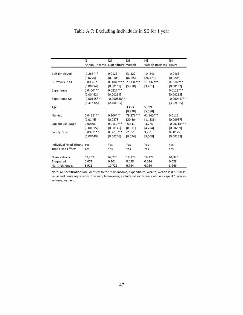
Table A.7: Excluding Individuals in SE for 1 year

[1] [2] [3] [4] [5]Annual Income Expenditure Wealth Wealth-­‐Business Hours

Self Employed -­‐0.288*** 0.0123 51,822 -­‐14,546 -­‐0.0465**[0.0270] [0.0103] [82,651] [26,473] [0.0205]

SE*Years in SE 0.00661* 0.00817*** 23,334*** 11,732*** 0.0102***[0.00354] [0.00165] [5,910] [3,201] [0.00182]

Experience 0.0400*** 0.0217*** 0.0123***[0.00462] [0.00264] [0.00255]

Experience Sq -­‐0.00115*** -­‐0.000538*** -­‐0.000417***[5.41e-­‐05] [2.40e-­‐05] [3.32e-­‐05]

Age 3,453 5,999[8,290] [5,580]

Married 0.0462*** 0.206*** 78,876*** 61,140*** 0.0116[0.0146] [0.0575] [20,404] [11,536] [0.00967]

Log spouse Wage 0.00505 0.0159*** -­‐6,441 -­‐3,775 -­‐0.00718***[0.00615] [0.00146] [8,311] [4,274] [0.00239]

Family Size 0.00971** 0.0615*** -­‐2,851 3,751 0.00175[0.00440] [0.00246] [8,074] [3,508] [0.00283]

Individual  Fixed  Effects Yes Yes Yes Yes YesTime  Fixed  Effects Yes Yes Yes Yes Yes

Observations 63,237 67,778 18,129 18,129 64,323R-squared 0.072 0.201 0.038 0.054 0.028No. Individuals 8,911 10,725 6,754 6,754 8,946

Note:  All  specifications  are  identical  to  the  main  income,  expenditure,  wealth,  wealth  less  business  value  and  hours  regressions.  The  sample  however,  excludes  all  individuals  who  only  spent  1  year  in  self-­‐employment.  

47

References

Aguiar, Mark A and Mark Bils, “Has Consumption Inequality Mirrored Income Inequality?,”

Technical Report, National Bureau of Economic Research 2011.

Aguiar, Mark and Erik Hurst, “Consumption versus Expenditure,” Journal of Political Economy,

2005, 113 (5), pp. 919–948.

Altonji, Joseph G. and Aloysius Siow, “Testing the Response of Consumption to Income Changes

with (Noisy) Panel Data,” The Quarterly Journal of Economics, 1987, 102 (2), pp. 293–328.

Andreoni, James, Brian Erard, and Jonathan Feinstein, “Tax Compliance,” Journal of Eco-

nomic Literature, 1998, 36 (2), pp. 818–860.

Blanchflower, David G., Andrew Oswald, and Alois Stutzer, “Latent entrepreneurship across

nations,” European Economic Review, 2001, 45 (4-6), 680 – 691.

Blundell, Richard, Luigi Pistaferri, and Ian Preston, “Imputing consumption in the PSID using

food demand estimates from the CEX,” The Institute for Fiscal Studies, UCL (University College

London), The Institute for Fiscal Studies, 2004.

Camerer, Colin and Dan Lovallo, “Overconfidence and Excess Entry: An Experimental Ap-

proach,” The American Economic Review, 1999, 89 (1), pp. 306–318.

Cooper, Arnold C., Carolyn Y. Woo, and William C. Dunkelberg, “Entrepreneurs’ perceived

chances for success,” Journal of Business Venturing, 1988, 3 (2), 97 – 108.

Evans, David S and Boyan Jovanovic, “An estimated model of entrepreneurial choice under

liquidity constraints,” The Journal of Political Economy, 1989, pp. 808–827.

Evans, David S. and Linda S. Leighton, “Some Empirical Aspects of Entrepreneurship,” The

American Economic Review, 1989, 79 (3), pp. 519–535.

48

Friedman, Milton, A Theory of the Consumption Function number frie57-1. In ‘NBER Books.’,

National Bureau of Economic Research, Inc, June 1957.

Gentry, William M and R Glenn Hubbard, “Tax policy and entrepreneurial entry,” The Ameri-

can Economic Review, 2000, 90 (2), 283–287.

Guo, Sheng, “The superior measure of PSID consumption: An update,” Economics Letters, 2010,

108 (3), 253 – 256.

Hall, Robert E., “Stochastic Implications of the Life Cycle-Permanent Income Hypothesis: The-

ory and Evidence,” The Journal of Political Economy, 1978, 86 (6), pp. 971–987.

and Frederic S. Mishkin, “The Sensitivity of Consumption to Transitory Income: Estimates

from Panel Data on Households,” Econometrica, 1982, 50 (2), pp. 461–481.

and Susan E. Woodward, “The Burden of the Nondiversifiable Risk of Entrepreneurship,” The

American Economic Review, 2010, 100 (3), pp. 1163–1194.

Hamilton, Barton H., “Does Entrepreneurship Pay? An Empirical Analysis of the Returns of

Self-Employment,” The Journal of Political Economy, 2000, 108 (3), pp. 604–631.

Hurst, Erik and Annamaria Lusardi, “Liquidity constraints, household wealth, and en-

trepreneurship,” Journal of political Economy, 2004, 112 (2), 319–347.

and Ben Pugsley, “The Non Pecuniary Benefits of Small Business Ownership,” University of

Chicago, working paper, 2010.

, Geng Li, and Benjamin Pugsley, “Are Household Surveys Like Tax Forms: Evidence from

Income Underreporting of the Self Employed,” Working Paper 16527, National Bureau of Eco-

nomic Research November 2010.

49

Jovanovic, Boyan, “Selection and the Evolution of Industry,” Econometrica: Journal of the

Econometric Society, 1982, pp. 649–670.

Kartashova, Katya, “The private equity premium puzzle revisited,” Technical Report, Bank of

Canada Working Paper 2011.

Lazear, Edward P., “Balanced Skills and Entrepreneurship,” The American Economic Review,

2004, 94 (2), pp. 208–211.

Meyer, Bruce D. and James X. Sullivan, “Front Matter,” The Journal of Human Resources, 2003,

38.

Moskowitz, Tobias J. and Annette Vissing-Jørgensen, “The Returns to Entrepreneurial Invest-

ment: A Private Equity Premium Puzzle?,” The American Economic Review, 2002, 92 (4), pp.

745–778.

Pissarides, Christopher A and Guglielmo Weber, “An expenditure-based estimate of Britain’s

black economy,” Journal of Public Economics, 1989, 39 (1), 17–32.

Puri, Manju and David T Robinson, “The Economic Psychology of Entrepreneurship and Fam-

ily Business,” Journal of Entrepreneurship and Management, 2013.

Quadrini, Vincenzo, “Entrepreneurship, saving, and social mobility,” Review of Economic Dy-

namics, 2000, 3 (1), 1–40.

Rosen, Harvey and Paul Willen, “Risk, Return and Self-Employment,” Chicago/Priceton Uni-

versity Discussion Paper, July 2002.

Roy, Andrew Donald, “Some thoughts on the distribution of earnings,” Oxford economic papers,

1951, pp. 135–146.

50

Skinner, Jonathan, “A superior measure of consumption from the panel study of income dynam-

ics,” Economics Letters, 1987, 23 (2), 213 – 216.

Slemrod, Joel, “Cheating Ourselves: The Economics of Tax Evasion,” The Journal of Economic

Perspectives, 2007, 21 (1), pp. 25–48.

51

8 Tables

Table I: Summary Statistics

[1] [2] [3] [4] [5] [6]

Paid Employees

Self Employed

Paid Employees

Self Employed

Only attempted wage-emp

Ever attempted self-emp

Experience 17.08 20.82 19.97 23.82 19.17 19.96(total years in labor force) [11.42] [10.80] [11.28] [10.68] [12.17] [11.5]Tenure 10.78 13.43 5.47 6.42 9.06 9.30(average years in each job) [7.73] [12.97] [5.48] [6.29] [6.91] [6.95]HS Drop 0.15 0.15 0.10 0.11 0.22 0.18(proportion of sample) [0.36] [0.36] [0.30] [0.31] [0.41] [0.39]HS Grad 0.35 0.24 0.35 0.33 0.35 0.29(proportion of sample) [0.47] [0.43] [0.47] [0.47] [0.48] [0.45]College Drop 0.27 0.28 0.27 0.24 0.25 0.26(proportion of sample) [0.45] [0.45] [0.44] [0.43] [0.43] [0.44]College Grad 0.12 0.17 0.15 0.14 0.10 0.14(proportion of sample) [0.32] [0.37] [0.36] [0.35] [0.29] [0.34]Grad School 0.11 0.17 0.08 0.12 0.08 0.12(proportion of sample) [0.31] [0.38] [0.27] [0.33] [0.26] [0.33]White 0.62 0.83 0.55 0.63 0.55 0.72(proportion of sample) [0.48] [0.37] [0.49] [0.48] [0.50] [0.45]Married 0.64 0.79 0.56 0.68 0.58 0.69(proportion of sample) [0.48] [0.41] [0.49] [0.47] [0.49] [0.46]Male 0.78 0.91 0.72 0.84 0.72 0.85(proportion of sample) [0.42] [0.29] [0.45] [0.37] [0.45] [0.36]Annual Hours Worked 1891 2190 2079 2097 1952 2109(average hours worked annually) [575.23] [865.28] [721.94] [963.09] [646] [838]Observations 4063 425 5571 707 16414 4261

Columns [1] to [4]: Summary of means in the cross sections, 1984 and 2005. Sample standard deviations in parentheses. Note that the number of observations for tenure in colum 1 is 2846, column 2 is 340, column 3 is 5115 and column 4 is 665. Experience and Annual hours worked are estimated off approximately (within 30 observations) the number of observations denoted in the "observations" row. All other variables are estimated from exactly the number of obsevations denoted in the "observations" row. Columns [5] and [6]: Summary of panel means. "Ever attempted self-employment" refers to individuals who have at some point appeared as self-employed in the PSID. "Only attempted wage employment" refers to individuals who have appeared as wage employed at some point in the PSID, but never as self-employed.

Panel Summary (1968-2005)

1984 2005

Cross Sectional Summary

52

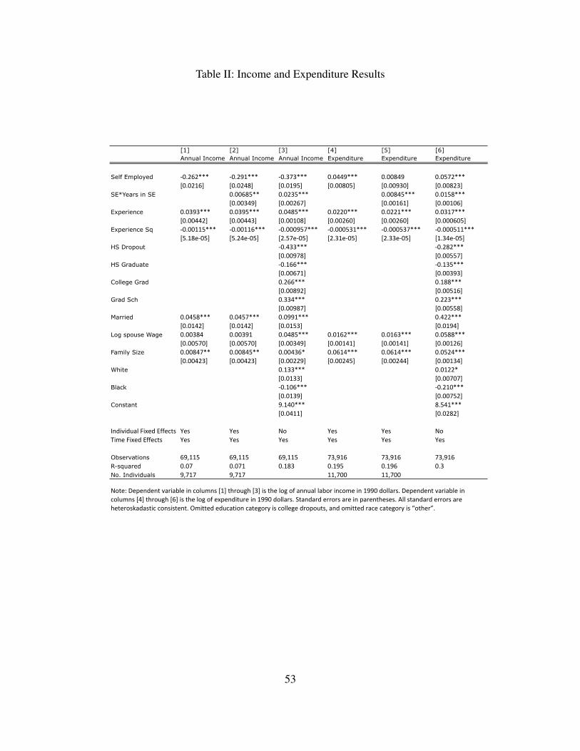
Table II: Income and Expenditure Results

[1] [2] [3] [4] [5] [6]Annual Income Annual Income Annual Income Expenditure Expenditure Expenditure

Self Employed -­‐0.262*** -­‐0.291*** -­‐0.373*** 0.0449*** 0.00849 0.0572***[0.0216] [0.0248] [0.0195] [0.00805] [0.00930] [0.00823]

SE*Years in SE 0.00685** 0.0235*** 0.00845*** 0.0158***[0.00349] [0.00267] [0.00161] [0.00106]

Experience 0.0393*** 0.0395*** 0.0485*** 0.0220*** 0.0221*** 0.0317***[0.00442] [0.00443] [0.00108] [0.00260] [0.00260] [0.000605]

Experience Sq -­‐0.00115*** -­‐0.00116*** -­‐0.000957*** -­‐0.000531*** -­‐0.000537*** -­‐0.000511***[5.18e-­‐05] [5.24e-­‐05] [2.57e-­‐05] [2.31e-­‐05] [2.33e-­‐05] [1.34e-­‐05]

HS Dropout -­‐0.433*** -­‐0.282***[0.00978] [0.00557]

HS Graduate -­‐0.166*** -­‐0.135***[0.00671] [0.00393]

College Grad 0.266*** 0.188***[0.00892] [0.00516]

Grad Sch 0.334*** 0.223***[0.00987] [0.00558]

Married 0.0458*** 0.0457*** 0.0991*** 0.422***[0.0142] [0.0142] [0.0153] [0.0194]

Log spouse Wage 0.00384 0.00391 0.0485*** 0.0162*** 0.0163*** 0.0588***[0.00570] [0.00570] [0.00349] [0.00141] [0.00141] [0.00126]

Family Size 0.00847** 0.00845** 0.00436* 0.0614*** 0.0614*** 0.0524***[0.00423] [0.00423] [0.00229] [0.00245] [0.00244] [0.00134]

White 0.133*** 0.0122*[0.0133] [0.00707]

Black -­‐0.106*** -­‐0.210***[0.0139] [0.00752]

Constant 9.140*** 8.541***[0.0411] [0.0282]

Individual  Fixed  Effects Yes   Yes   No   Yes   Yes   NoTime  Fixed  Effects Yes   Yes   Yes   Yes   Yes   Yes  

Observations 69,115 69,115 69,115 73,916 73,916 73,916R-squared 0.07 0.071 0.183 0.195 0.196 0.3No. Individuals 9,717 9,717 11,700 11,700

Note:  Dependent  variable  in  columns  [1]  through  [3]  is  the  log  of  annual  labor  income  in  1990  dollars.  Dependent  variable  in  columns  [4]  through  [6]  is  the  log  of  expenditure  in  1990  dollars.  Standard  errors  are  in  parentheses.  All  standard  errors  are  heteroskadastic  consistent.  Omitted  education  category  is  college  dropouts,  and  omitted  race  category  is  “other”.  

53

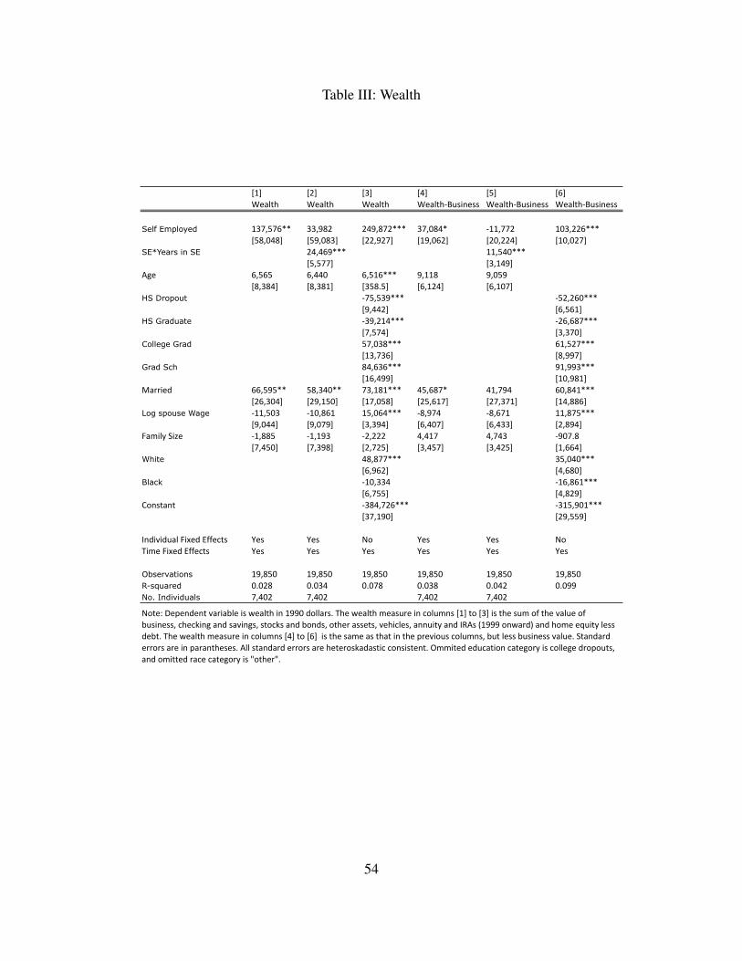
Table III: Wealth

[1] [2] [3] [4] [5] [6]Wealth Wealth Wealth   Wealth-­‐Business Wealth-­‐Business Wealth-­‐Business

Self Employed 137,576** 33,982 249,872*** 37,084* -­‐11,772 103,226***[58,048] [59,083] [22,927] [19,062] [20,224] [10,027]

SE*Years in SE 24,469*** 11,540***[5,577] [3,149]

Age 6,565 6,440 6,516*** 9,118 9,059[8,384] [8,381] [358.5] [6,124] [6,107]

HS Dropout -­‐75,539*** -­‐52,260***[9,442] [6,561]

HS Graduate -­‐39,214*** -­‐26,687***[7,574] [3,370]

College Grad 57,038*** 61,527***[13,736] [8,997]

Grad Sch 84,636*** 91,993***[16,499] [10,981]

Married 66,595** 58,340** 73,181*** 45,687* 41,794 60,841***[26,304] [29,150] [17,058] [25,617] [27,371] [14,886]

Log spouse Wage -­‐11,503 -­‐10,861 15,064*** -­‐8,974 -­‐8,671 11,875***[9,044] [9,079] [3,394] [6,407] [6,433] [2,894]

Family  Size -­‐1,885 -­‐1,193 -­‐2,222 4,417 4,743 -­‐907.8[7,450] [7,398] [2,725] [3,457] [3,425] [1,664]

White 48,877*** 35,040***[6,962] [4,680]

Black -­‐10,334 -­‐16,861***[6,755] [4,829]

Constant -­‐384,726*** -­‐315,901***[37,190] [29,559]

Individual  Fixed  Effects Yes Yes No   Yes Yes No  Time  Fixed  Effects Yes Yes Yes Yes Yes Yes

Observations 19,850 19,850 19,850 19,850 19,850 19,850R-squared 0.028 0.034 0.078 0.038 0.042 0.099No. Individuals 7,402 7,402 7,402 7,402

Note:  Dependent  variable  is  wealth  in  1990  dollars.  The  wealth  measure  in  columns  [1]  to  [3]  is  the  sum  of  the  value  of    business,  checking  and  savings,  stocks  and  bonds,  other  assets,  vehicles,  annuity  and  IRAs  (1999  onward)  and  home  equity  less  debt.  The  wealth  measure  in  columns  [4]  to  [6]    is  the  same  as  that  in  the  previous  columns,  but  less  business  value.  Standard  errors  are  in  parantheses.  All  standard  errors  are  heteroskadastic  consistent.  Ommited  education  category  is  college  dropouts,  and  omitted  race  category  is  "other".  

54

Table IV: Variance in expenditure and wealth

[1] [2] [3]Residual Squared Expenditure

Residual Squared Wealth

Residual  Squared  Wealth  (trans)

Self Employed 9.89E-­‐05 4.972e+11* -­‐5.786[0.00511] [2.891e+11] [58.90]

SE/Tenure 0.0115 -­‐5.909e+11* 23.62[0.00736]

Experience -­‐0.00393***[0.00145]

Experience Sq 8.44e-­‐05***[1.10e-­‐05]

Age 5.71E+10 17.97[3.573e+10] [13.28]

Married -­‐0.139* 7.28E+10 -­‐73.62[0.0714] [6.707e+10] [47.14]

Log spouse Wage -­‐0.00231*** -­‐4.73E+10 -­‐4.779[0.000791] [3.801e+10] [7.942]

Family Size -­‐0.0015 -­‐1.09E+10 -­‐11.23*[0.00121] [2.003e+10] [6.144]

Individual  Fixed  Effects Yes Yes YesTime  Fixed  Effects Yes Yes Yes

Observations 73,916 19,850 19,850R-squared 0.007 0.002 0.004No. Individuals 11,700 7,402 7,402

Note: Dependent variables are the squared residuals from the main fixed effects expenditure regression(column [5] of Table 5), wealth regression(column [2] of Table 6) and wealth transformed regression (column [2] of Table 13). Standard errors are in parentheses. All standard errors are heteroskadastic consistent.

55

Tabl

eV

:Pre

caut

iona

ryB

ehav

ior

[1]

[2]

[3]

[4]

[5]

[6]

[7]

[8]

[9]

Expe

nditu

reExpe

nditu

reExpe

nditu

reWealth

 Wealth

Wealth

Wealth

-­‐BusinessWealth

-­‐BusinessWealth

-­‐Business

Before  SE

-­‐0.005

88-­‐5.117***

-­‐0.981

[0.0109]

[1.334]

[1.129]

Two  Year  Prec

-­‐0.018

40.811

0.695

[0.0139]

[2.811]

[2.805]

One

 Year  P

rec

-­‐0.018

3.756

3.671

[0.0133]

[2.562]

[2.524]

Log  Spou

se  W

age

0.0214***

0.0193***

0.0195***

0.569

0.417

0.324

0.543

0.701

0.61

[0.00278]

[0.00532]

[0.00532]

[0.514]

[1.609]

[1.593]

[0.457]

[1.640]

[1.626]

Family  Size

0.102***

0.0923***

0.0922***

2.011***

3.084***

3.004***

2.227***

2.837***

2.757***

[0.00403]

[0.00763]

[0.00762]

[0.485]

[0.999]

[1.004]

[0.427]

[0.991]

[0.997]

Marrie

d0.187**

00

10.67

00

7.112

00

[0.0918]

[0]

[0]

[11.58]

[0]

[0]

[11.36]

[0]

[0]

Individu

al  Fixed

 Effe

cts

Yes

Yes

Yes

Time  Fixed  Effects

Yes

Yes

Yes

Observatio

ns23,370

8,553

8,553

5762

1264

1264

5762

1264

1264

R-­‐squared

0.207

0.177

0.177

0.143

0.12

0.123

0.154

0.114

0.118

No.  Individu

als

2,883

1,716

1,716

1973

757

757

1973

757

757

Note:  Dep

ende

nt  variable  in  colum

ns  [1

]  -­‐  [3

]  is  log  of  total  expen

ditures,  colum

ns  [4

]  -­‐  [6

]  is  w

ealth

 cub

e  root  transformed

 and

 colum

ns  [7

]  -­‐  [9

]  is  w

ealth

 less  

busin

ess  v

alue

 cub

e  root  transformed

.  All  de

pend

ent  variables  are  in  1990  do

llars.  Colum

ns  1,  4  and

 7  includ

e  all  observatio

ns  before,  during  and  after  S

E.  "B

efore  

SE"  takes  on  a  du

mmy  value  of  1  fo

r  all  pe

riods  prio

r  to  en

terin

g  SE  fo

r  the

 first  tim

e  for  ind

ividuals  who

 eventually  sw

itch  into  SE  and  a  0  in  all  pe

riods  th

ereafter,  

includ

ing    while  se

lf-­‐em

ployed

 and

 after  leaving  self-­‐em

ploymen

t.  Co

lumns  2,  3,  5,  6,  8  and

 9  only  includ

e  ob

servations  from

 those  years  p

rior  to  en

try  into  se

lf-­‐em

ploymen

t.  "O

ne  Year  P

rec"  ta

kes  o

n  a  du

mmy  value  of  1  in  th

e  on

e  year  prio

r  to  en

try  into  SE.  "T

wo  Year  Prec"  ta

kes  o

n  a  du

mmy  value  of  1  in  each  of  th

e  tw

o  years  p

rior  to  en

try  into  SE.    Stand

ard  errors  are  in  parantheses.  A

ll  standard  errors  a

re  heteroskadastic  con

sistent.

56

Table VI: Switching Out of Self-Employment

[1] [2] [3] [4]Expenditure Expenditure Annual  Income Annual  Income

A3er  SE -­‐0.0520*** -­‐0.0382** -­‐0.256*** -­‐0.664***[0.0161] [0.0174] [0.0286] [0.139]

A3er  SE*Yrs  Sch 0.0307***[0.0105]

Experience 0.0212*** 0.0338***[0.00399] [0.00737]

Experience Sq -­‐0.000495*** -­‐0.00111***[5.55e-­‐05] [0.000107]

Log spouse Wage 0.0277*** 0.0279*** -­‐0.00835 -­‐0.00815[0.00379] [0.00402] [0.00710] [0.00708]

Family Size 0.100*** 0.102*** 0.00341 0.00254[0.00488] [0.00478] [0.00865] [0.00856]

Individual  Fixed  Effects Yes Yes Yes YesTime  Fixed  Effects Yes Yes Yes Yes

ObservaMons 15,292 12,751 13,008 12,983R-­‐squared 0.188 0.222 0.08 0.083Number  of  id 2,354 2,137 1,960 1,953

Note:  Dependent  variable  in  columns  [1]  and  [2]  is  the  log  of  expenditure  in  1990  dollars.  Dependent  variable  in  columns  [3]  and  [4]  is  the  log  of  the  household  head's  annual  income  in  1990  dollars.  Fixed  effects  (FE)  are  at  the  individual  level.  ''A3er  SE''  takes  on  a  value  of  1  in  all  years  a3er  an  individual  first  enters  self-­‐employment  but  does  not  appear  self-­‐employed.  Column  [1]  includes  all  individuals  regardless  of  whether  they  return  to  wage  employment  or  if  they  leave  the  labor  force.  Columns  [2],  [3]  and  [4]  only  include  those  Mme  periods  when  one  returns  to  wage  work.    Standard  errors  are  in  parentheses.  All  standard  errors  are  heteroskadasMc  consistent.  

57

Table VII: Hours Worked

[1] [2] [3]Hours Hours Hours

Self Employed 0.0320*** -0.0642*** -0.0119[0.0110] [0.0182] [0.0124]

SE*Years in SE 0.0115*** 0.00958***[0.00170] [0.000765]

Experience 0.0126*** 0.0123*** 0.00793***[0.00244] [0.00243] [0.000677]

Experience Sq -0.000432*** -0.000426*** -­‐0.000237***[3.23e-05] [3.21e-05] [1.63e-05]

Married 0.0133 0.0134 0.0304***[0.00969] [0.00967] [0.00950]

Log spouse Wage -0.00804*** -0.00799*** 0.0015[0.00228] [0.00228] [0.00159]

Family Size 0.000452 0.000385 0.00403***[0.00271] [0.00270] [0.00143]

HS Dropout -­‐0.0484***[0.00636]

HS Graduate -­‐0.0112***[0.00408]

College Grad 0.0181***[0.00476]

Grad Sch -­‐0.00557[0.00555]

White 0.0156**[0.00766]

Black -­‐0.0442***[0.00829]

Constant 7.574***[0.0226]

Individual  Fixed  Effects Yes Yes NoTime  Fixed  Effects Yes Yes Yes

Observations 70,233 70,233 70,233R-squared 0.026 0.027 0.034No. Individuals 9,756 9,756

Note:  Dependent  variable  is  the  log  of  annual  hours  worked.  Standard  errors  are  in  parentheses.  All  standard  errors  are  heteroskadastic  consistent.  Omitted  education  category  is  college  dropouts,  and  omitted  race  category  is  “other”.  

58

9 Figures

Figure I: Responsiveness of Expenditure to Reported Income

Notes: This graph plots the responsiveness of expenditure to reported income (household head’s labor income) by income quartile as defined by

wage-earners who have never attempted self-employment. The graph shows that prior to entering self-employment (triangular points), those who

eventually do, display expenditure responses to changes in reported income that are almost identical to that of individuals who are only ever wage-

employed (square points). Once in self-employment, expenditure becomes substantially less responsive to reported income (circular points). Upon

returning to wage-employment (diamond points), expenditure responses once again mirror that of those who are only ever wage employed (square

points), with the exception of those corresponding to the 75th percentile. The premise underlying this graph is that wage-employed individuals

are least plagued by income measurement problems, and therefore serve as the baseline for comparison. This graph indicates that those who try

self-employment respond to income changes in a very similar manner to those who are only ever wage-employed, except for those periods when

they are self-employed. This suggests that income measurement in self-employment, rather than differences in preferences and behaviors, is what

drives this difference in responsiveness. The quartiles are defined by cutting household head’s labor income (in 1990 dollars) into the 25th, 50th

and 75th quartiles using only individuals who have ever been wage employed between 1968 - 1997. These quartile values are then applied to those

who have “ever been self-employed” where observations are split into“being wage employed prior to self employment” (triangular points), “being

59

self-employed” (circular points) and “being wage-employed after first entry into self-employment” (diamond points). The points in the plot are

obtained from running regressions of the log of consumption against the log of head’s annual income (both in 1990 dollars including individual and

time fixed effects) for the four separate categories described above, by income quartiles as defined above. All coefficients from these estimations

are significant at the five percent level, and most are significant at the one percent level.

60