THE SOURCES OF PRODUCTIVITY CHANGE IN THE MANUFACTURING

SECTORS OF THE U.S. ECONOMY

by

Christopher J. O’Donnell

Centre for Efficiency and Productivity Analysis,

The University of Queensland, Brisbane 4072, Australia

First Version: 30 August 2011

This Version: 14 September 2011

Abstract: The U.S. Bureau of Labor Statistics measures productivity change using an

index formula that fails a transitivity test. This means the Bureau is likely to report

productivity changes even when outputs and inputs in different (non-adjacent) periods

are identical. I use alternative formulas that a) satisfy all economically-relevant tests

from index theory and b) can be decomposed into measures of technical change and

efficiency change. I find the main sources of productivity change are scale and mix

efficiency change. This supports the view that most firms are technically efficient and

rationally change their production plans in response to changes in prices.

KEYWORDS: Data Envelopment Analysis, Malmquist Index, Lowe Index, Färe-

Primont Index, Geometric Young Index, Mix Efficiency

1. Introduction

Well-known drivers of productivity change include technical change and changes in measures

of technical and scale efficiency (e.g., Nishimizu and Page (1982)). Technical change is

essentially a measure of movements in the production frontier associated with changes in the

stock of scientific knowledge and/or other characteristics of the production environment.

Technical efficiency change is a measure of movements towards or away from the frontier,

almost always associated with the adoption of new technologies and/or changes in the number

of errors made during the production process. Scale efficiency change is a measure of

movements around the frontier surface, often in response to changes in relative prices and/or

other production incentives.

There are at least two reasons for wanting to identify the drivers of productivity change.

First, all other things being equal, productivity growth that is driven by technical progress

and/or increases in technical efficiency will always be associated with higher net returns.

However, as I explain later in the paper, productivity growth that is driven by increases in

scale efficiency will often be associated with lower net returns. Thus, identifying the technic-

al change and efficiency change components of productivity change is critically important for

determining whether productivity growth is associated with higher or lower net returns (and

welfare). Second, different policies will generally have different effects on the different

components of productivity change. For example, research and development (R&D) policies

can be expected to have a larger effect on rates of technical change than on levels of scale

efficiency. Similarly, policies designed to move firms1 closer to the best-practice frontier

(e.g., education and training programs) or increase levels of scale efficiency (e.g., changes in

taxes and subsidies) are unlikely to increase productivity if firms are already fully technically

efficient and operating at an optimal scale.

1 The term ‘firms’ is used generically in reference to decision-making units (e.g., individuals, industries, states,

regions, countries).

2

In an influential2 paper in the American Economic Review, Färe et al. (1994) use data

envelopment analysis (DEA) to estimate and decompose the Malmquist productivity index of

Caves, Christensen and Diewert (1982a, p. 1404). DEA estimation and decomposition of

Malmquist indexes is now widespread in the productivity literature (Lovell (2003, p. 438)).

This is unfortunate because, except in restrictive special cases, DEA estimates of Malmquist

indexes are unreliable measures of productivity change. To demonstrate, later in this paper I

provide an example where a firm is able to produce the same output using fewer inputs and

yet the DEA estimate of the Malmquist index indicates that productivity is unchanged.

The widespread use of DEA to estimate Malmquist indexes can be attributed to three

main factors. First, it can be computed without the need for price data – all that is needed is

an estimate of the production technology. However, there are now at least two other indexes

that can also be used to measure productivity change without the need for price data – a

Hicks-Moorsteen index3 proposed by Bjurek (1996) and a Färe-Primont index4 proposed by

O'Donnell (2011). Like the Malmquist index, these productivity indexes require an estimate

of the production technology. In the simple example mentioned above, where a firm produc-

es the same output using less input, DEA estimates of the Hicks-Moorsteen and Färe-Primont

indexes quite sensibly indicate that productivity has increased.

Second, Färe et al. (1994) show that the Malmquist index can be decomposed into a

measure of technical change and a measure of technical efficiency change. Indeed, until

recently it seemed that the Malmquist index was the only productivity index that could be

exhaustively decomposed into the measures of technical change and efficiency change that

policy-makers need. However, O'Donnell (2008) has recently demonstrated that all theoreti-

cally-meaningful productivity indexes can be exhaustively decomposed into such measures.

2 The paper has been cited more than 660 times since 1996 (Scopus). 3 The name ‘Hicks-Moorsteen’ has been used by Färe, Grosskopf and Roos (1996), Briec and Kerstens (2004)

and Briec and Kerstens (2011). This usage derives from the fact that the index is the geometric average of two productivity indexes that Diewert (1992, p. 240) attributes to Hicks (1961) and Moorsteen (1961). However, Nemoto and Goto (2005) refer to the index as a Hicks-Moorsteen-Bjurek index.

4 I refer to the O'Donnell (2011) index as a ‘Fare-Primont’ index because it can be written as the ratio of two

indexes defined by Färe and Primont (1995, p. 36, 38).

3

In the simple example mentioned above, the estimated increases in the Hicks-Moorsteen and

Färe-Primont indexes can be fully attributed to increases in scale and mix efficiency (i.e.,

economies of scale and scope). Grifell-Tatjé and Lovell (1995) argue that, irrespective of

how it is estimated, the Malmquist index ignores productivity changes associated with

changes in scale. Later in this paper I provide evidence that DEA estimates of the Malmquist

index may also fail to capture productivity changes associated with changes in scope (i.e.,

changes in output mix and input mix).

Finally, Lovell (2003, p. 438) attributes the popularity of the Malmquist index in part to

the fact that DEA linear programs for computing and/or decomposing it have been incorpo-

rated into at least two software packages. The DEAP 2.1 software is especially popular

because it is available free-of-charge. In this paper I develop DEA linear programs for

computing and decomposing Hicks-Moorsteen and Färe-Primont indexes. These linear

programs have recently been incorporated into an edition of the DPIN 3.0 software that is

also available free-of-charge.

Within the large class of productivity indexes that can be broken into recognizable

components, some indexes are more reliable than in others. For example, the Färe-Primont

index can be used to make reliable multi-lateral and multi-temporal comparisons (i.e., com-

parisons involving many firms and time periods) but the Hicks-Moorsteen index can only be

used to make reliable binary comparisons (i.e., comparisons involving only two firms or two

time periods). This is because the Hicks-Moorsteen index fails the transitivity test of Fisher

(1922). Transitivity means that a direct comparison of the productivity of two firms/periods

will yield the same estimate of productivity change as an indirect comparison through a third

firm/period. To illustrate the importance of transitivity, later in this paper I consider a simple

case where a firm uses the same inputs to produce the same outputs in two different periods.

A direct comparison of the two observations plausibly yields a Hicks-Moorsteen index value

of one, indicating that productivity is unchanged, but an indirect comparison through a third

4

observation yields a value of 1.18, indicating that productivity has increased by 18%. In

contrast, direct and indirect comparisons using the Färe-Primont index yield index values of

one.

If prices are available then the menu of available productivity indexes expands to include

Törnqvist and Fisher indexes. The Törnqvist index is widely used in the growth accounting

literature where it is better known as the Solow residual (see Timmer, O'Mahony and van Ark

(2007, p. 65)). It is also used by the Bureau of Labor Statistics (BLS) to measure manufactur-

ing sector productivity growth. The Fisher index is used by several statistical agencies,

including the US Department of Agriculture (USDA) and the Australian Bureau of Agricul-

tural and Resource Economics (ABARE), to measure farm sector productivity growth.

Unfortunately, neither of these two indexes is transitive, so they can only be used to make

binary comparisons. To make multi-lateral or multi-temporal comparisons, it is common to

compute transitive versions of the Törnqvist and Fisher indexes using a geometric averaging

procedure due to Elteto and Koves (1964) and Szulc (1964). However, although they may be

transitive, these so-called Törnqvist-EKS and Fisher-EKS indexes5 fail another fundamentally

important property of index numbers – the identity axiom. The identity axiom says that if

two firms produce the same outputs using the same inputs then the index should take the

value one (i.e., indicate that the firms are equally productive). In this paper I provide an

example where two firms choose exactly the same output-input combinations but the Fisher-

EKS and Törnqvist-EKS indexes take values ranging from 0.97 to 1.17. In contrast, the Färe-

Primont index satisfies both the identity axiom and the transitivity test and takes the value

one. If prices are available then at least two other indexes also satisfy the identity axiom and

the transitivity test and so can also be used for multi-lateral and multi-temporal comparisons.

One of these is the Lowe productivity index proposed by O'Donnell (2010b), and the other is

a Geometric Young index that has not yet received any attention in the productivity literature.

5 The Fisher-EKS index is also known simply as the EKS index (e.g., Fox (2003)). The Tornquist-EKS index

was first proposed by Caves, Christensen and Diewert (1982b, p. 78) and is also known as the CCD index or the generalized Theil-Törnqvist index (e.g., Pilat and Rao (1996, p. 119)).

5

In this paper I compute Färe-Primont, Lowe and Geometric Young productivity indexes

for eighteen manufacturing sectors of the US economy for the period 1987 to 2008. I also

decompose the Färe-Primont index into various technical change and efficiency change

components. Until now, the Färe-Primont productivity index has only been computed and

decomposed using Bayesian econometric methods (see O'Donnell (2011)). An advantage of

the Bayesian approach is that it is possible to draw valid finite-sample inferences concerning

rates of productivity growth and measures of technical change, technical efficiency change

and scale-mix efficiency change. However, it is difficult to estimate levels of (and, for that

matter, changes in) pure scale efficiency (i.e., the productivity gains associated with changes

in scale alone) and pure mix efficiency (i.e., the gains associated with changes in scope

alone). The Lowe productivity index has only ever been decomposed using DEA methodol-

ogy (see O'Donnell (2010b)). In this paper I develop similar DEA methodology for compu-

ting and decomposing Färe-Primont indexes. The DEA approach has been chosen over the

Bayesian approach, not just because it can be used to identify levels of pure scale and mix

efficiency, but because it doesn’t require any explicit assumptions about random variables

representing statistical noise. Such assumptions are unnecessary because DEA implicitly

assumes that all noise effects are zero. Because there are no noise effects, DEA side-steps an

endogeneity problem6 that often arises in the econometric estimation of multiple-input mul-

tiple-output technologies.

The structure of the paper is as follows. In Section 2 I present several productivity index

number formulas, three of which – the Färe-Primont, Lowe and Geometric Young indexes –

satisfy all economically-relevant axioms and tests from index number theory. These three

indexes are members of a class of “multiplicatively-complete” productivity indexes. In

Section 3 I outline the relationship between profitability change, productivity change and

changes in relative prices. Among other things, I explain why falls in productivity are often

associated with higher net returns. In Section 4 I explain that all multiplicatively-complete 6 See Atkinson, Cornwell and Honerkamp (2003, p. 288).

6

productivity indexes can be decomposed into a measure of technical change and several

measures of efficiency change. The efficiency measures include a measure of overall produc-

tive efficiency and several measures of technical, scale and mix (or scope) efficiency. In

Section 5 I show how all of these components can be estimated using DEA methodology.

Among other things, I reveal that DEA estimates of Hicks-Moorsteen and Färe-Primont MFP

indexes can be viewed as Fisher and Lowe MFP indexes but with support (or shadow) prices

used in place of observed market prices. In Section 6 I use BLS data to estimate levels of

MFP and efficiency in US manufacturing. In Section 7 I summarize the paper and suggest

directions for further research.

2. Measuring Multi-factor Productivity Change

The productivity of a single-output single-input firm is almost always defined as the output-

input ratio7. O'Donnell (2008) generalizes this concept to the multiple-output multiple-input

case by formally defining productivity to be the ratio of an aggregate output to an aggregate

input. Consider a dataset containing observations on N firms over T time periods and let

1( ,..., )it it Jitq q q and 1( ,..., )it it Kitx x x denote the output and input vectors of firm i in period

t. O'Donnell (2008) defines the multi-factor productivity8 (MFP) of the firm as

/it it itMFP Q X where ( )it itQ Q q is an aggregate output, ( )it itX X x is an aggregate

input, and Q(.) and X(.) are non-negative non-decreasing linearly-homogeneous aggregator

functions. With this definition, the index that compares the MFP of firm i in period t with the

MFP of firm h in period s is

(1) ,,

,

/ /

/ /hs itit it it it hs

hs iths hs hs it hs hs it

QMFP Q X Q QMFP

MFP Q X X X X

where , /hs it it hsQ Q Q and , /hs it it hsX X X are output and input quantity indexes respective-

7 It is also possible to define productivity as the output minus the input. However, this alternative measure is

generally regarded as unsatisfactory because it is sensitive to units of measurement. 8 O'Donnell (2008) uses the term total factor productivity (TFP) instead of multi-factor productivity (MFP).

Statistical agencies such as the BLS often prefer the latter terminology in view the fact that multiple, but not all, factors of production are accounted for in the analysis.

7

ly. Equation (1) expresses MFP growth as a measure of output growth divided by a measure

of input growth, which is how most economists define productivity change (e.g., Jorgenson

and Griliches (1967)).

Productivity indexes that can be written in terms of aggregate quantities as in equation (1)

are said to be multiplicatively-complete (O'Donnell (2008)). An example of a multiplicative-

ly complete MFP index is the Hicks-Moorsteen index (e.g., Briec and Kerstens (2011, p.

768)):

(2)

1/2

,

( , , ) ( , , ) ( , , ) ( , , )

( , , ) ( , , ) ( , , ) ( , , )O hs it O it it I hs hs I hs it

hs itO hs hs O it hs I it hs I it it

D x q s D x q t D x q s D x q tMFP

D x q s D x q t D x q s D x q t

where ( , , ) max { 0:OD x q t x can produce q in period t} and ( , , )ID x q t

max { 0: x can produce q in period t} are the Shephard (1953) output and input dis-

tance functions representing the period-t production technology. The output and input aggre-

gator functions underpinning the Hicks-Moorsteen index are ( )Q q

1/ 2( , , ) ( , , )O hs O itD x q s D x q t and 1/ 2

( ) ( , , ) ( , , ) .I hs I itX x D x q s D x q t One of the attractive

features of the Hicks-Moorsteen index is that can be computed without having to collect price

data. Thus, it can be used in non-competitive industries where input and output prices may be

unavailable. However, it can only be computed by assuming (or estimating) a functional

representation of the production technology. A related index that also requires knowledge of

the production technology is the output-oriented9 Malmquist MFP index (e.g., Caves et al.

(1982a, p. 1404), Färe et al. (1994, p. 70)):

(3) 1/ 2

,

( , , ) ( , , ).

( , , ) ( , , )O it it O it it

hs itO hs hs O hs hs

D x q s D x q tMFP

D x q s D x q t

Except in restrictive special cases, this index cannot be expressed in terms of aggregate

quantities (i.e., it is not multiplicatively complete) nor as an output index divided by an input

index (i.e., it is not a recognizable measure of MFP change). One special case is when the

technology is input-homothetic and exhibits constant returns to scale (CRS). In this case, the

9 An analogous input-oriented Malmquist productivity index is also available.

8

Hicks-Moorsteen and Malmquist MFP indexes both collapse to the same combined measure

of technical change and technical efficiency change (Färe et al. (1996)). A second special

case is when the technology exhibits CRS and there is no technical change. In this case it is

easily shown that the Hicks-Moorsteen and Malmquist MFP indexes both collapse to a

measure of technical efficiency change. These special cases suggest that the output-oriented

Malmquist MFP index is an unreliable measure of productivity change unless the production

technology exhibits CRS. In empirical practice, it is common to impose the CRS assumption

even if the true technology exhibits variable returns to scale (VRS).

To illustrate the importance of multiplicative completeness, consider two firms that have

access to the same single-input single-output production technology. Suppose that Firm A

uses 6 units of input to produce 6 units of output, while Firm B uses 4 units of input to pro-

duce 3 units of output. If productivity is defined as the output-input ratio then the MFP of

Firm A is 6/ 6 1,AMFP the MFP of Firm B is 3/ 4 0.75,BMFP and the index that

compares the MFP of the two firms (using Firm A as the reference firm) is

/ 0.75/1 0.75.AB B AMFP MFP MFP All multiplicatively-complete MFP indexes will take

the value 0.75, indicating that Firm B is 25% less productive than Firm A. However, the

Malmquist MFP index will take a value that depends on the assumed (or estimated) form of

the production technology. Four cases are illustrated in panels a) to d) in Figure 1. Panel a)

depicts a case where the technology (the solid curve) exhibits variable returns to scale (VRS)

and both firms are fully technically efficient – in this case the Malmquist MFP index takes the

value one, indicating that both firms are equally productive. Panel b) depicts a case where the

technology exhibits decreasing returns to scale (DRS) and Firm B is only producing 60% of

the output that is feasible using 4 units of input – in this case the Malmquist index takes a

value 0.6. Panel c) depicts a case where the technology exhibits increasing returns to scale

(IRS) and Firm A is only producing 75% of the output that is feasible using 6 units of input –

in this case the Malmquist index takes a value 1.33. Finally, panel d) depicts a case where

9

the technology exhibits CRS, Firm B is only producing 56.25% of the output that is feasible

using 4 units of input and Firm A is only producing 75% of the output that is feasible using 6

units of input – in this case the Malmquist index takes a value 0.5625/0.75 = 0.75, indicating

(correctly) that Firm B is 25% less productive than Firm A. This last panel illustrates that if

the technology exhibits CRS and there is no technical change then the Malmquist and Hicks-

Moorsteen indexes are both equal to a measure of technical efficiency change (i.e., the second

special case mentioned above).

Different non-negative non-decreasing linearly-homogeneous aggregator functions yield

different multiplicatively-complete MFP indexes. Examples of aggregator functions and

associated productivity indexes that can be used for binary comparisons (i.e., comparisons

involving only two observations) are presented in Table 1. In this table,

1( ,..., ) 0it it Jitp p p and 1( ,..., ) 0it it Kitw w w are vectors of output and input prices, and

1( ,..., ) 0it it Kitr r r and 1( ,..., ) 0it it Kits s s are vectors of income and cost shares.

O’Donnell (2008) refers to the aggregator functions in the first three rows of Table 1 as

Laspeyres, Paasche and Fisher functions because they yield output and input quantity indexes

that are well-known by those names. The aggregator functions in rows four and five are

referred to in this paper as Malmquist-hs and Malmquist-it functions because they yield the

firm-specific (and/or period-specific) Malmquist output and input quantity indexes of Caves

et al. (1982a, p. 1399-1400). The aggregator functions in row six are the geometric averages

of the Malmquist-hs and Malmquist-it functions and are referred to in this paper as Hicks-

Moorsteen functions because they yield the Hicks-Moorsteen MFP index defined by equation

(2). Finally, the aggregator functions in rows seven and eight yield quantity indexes that

have received little, if any, attention in the productivity literature. In this paper I refer to them

as Törnqvist functions because their geometric averages, given in the last row, yield well-

known Törnqvist output, input and productivity indexes.

Index formulas are often selected according to whether or not they satisfy certain axioms

10

and tests. In the case of the input quantity index , ( ) / ( ) ( , ),hs it it hs hs itX X x X x X x x for

example, the economically-relevant10 axioms and tests are11:

A.1 Monotonicity axiom: ( , ) ( , )hs it hs grX x x X x x if it grx x and ( , ) ( , )hs it gr itX x x X x x if

.gr hsx x

A.2 Linear homogeneity axiom: ( , ) ( , )hs it hs itX x x X x x for 0.

A.3 Identity axiom: ( , ) 1.it itX x x

A.4 Homogeneity of degree 0 axiom: ( , ) ( , )hs it hs itX x x X x x for 0.

A.5 Commensurability axiom: ( , ) ( , )hs it hs itX x x X x x where is a diagonal matrix

with diagonal elements strictly greater than 0.

A.6 Proportionality axiom: ( , )hs hsX x x for 0.

T.1 Transitivity test: , , , .hs it hs gr gr itX X X

T.2 Time-space reversal test: , ,1/hs it it hsX X

Axiom A.1 (monotonicity) says that the index increases with increases in any element of the

comparison vector itx and with decreases in any element of the base (or reference) vector

.hsx Axiom A.2 (linear homogeneity) says that a proportionate increase in the comparison

vector will cause the value of the index to increase by the factor of proportionality. Axiom

A.3 (identity) says that if the comparison and base vectors are identical then the index number

is equal to one. Axiom A.4 (homogeneity of degree 0) says that multiplication of the compar-

ison and reference vectors by the same constant will leave the index number unchanged.

Axiom A.5 (commensurability) says the index number is robust to changes in units of mea-

surement. Axiom A.6 (proportionality) says that if the reference vector is proportionate to

the base vector then the index number is equal to the factor of proportionality. Test T.1

(transitivity) says the index number that directly compares the inputs of a comparison

10 Other index number tests listed by Eichhorn (1976, p. 248-249) are mathematically convenient but are not

directly relevant to the economic measurement of quantity change or productivity change. 11

Let jitx denote the j-th element of .itx The notation hs itx x means that jhs jitx x for all 1,...,j J and there

exists at least one value 1,...,j J where .jhs jitx x

11

firm/period with the inputs of a base firm/period is identical to the index number computed

when the comparison is made through an intermediate firm/period. Finally, Test T.2 (time

and space reversal) says that the index comparing the inputs of a comparison firm/period with

the inputs of a base firm/period is the inverse of the index obtained when the input vectors are

interchanged. Output quantity indexes and MFP indexes must satisfy an analogous set of

commonsense axioms and tests.

To illustrate the practical relevance of these axioms and tests, consider an industry in

which firms use two inputs to produce a single output. Hypothetical price and quantity data

for four firms in two periods are given in Table 2. Observe that firms 1 to 3 have chosen the

same input-output combinations in period 2 as they chose in period 1. Thus, MFP indexes

should indicate that these three firms were just as productive in period 2 as they had been in

period 1 (i.e., the identity axiom should ensure 1, 2 1i iMFP for 1, 2,3).i Also observe that

firm 4 produced the same output in both periods, but used a smaller input vector in period 2

than it had used in period 1 (it used the same amount of input 2, but 20% less of input 1).

With this reduction in input use, MFP indexes should indicate that firm 4 was more produc-

tive in period 2 than in period 1 (i.e., the monotonicity axiom should ensure that 41,42 1).MFP

Table 3 reports Malmquist, Hicks-Moorsteen, Fisher and Törnqvist indexes measuring

MFP change for each of the four firms. Both the Malmquist and Hicks-Moorsteen index

values were obtained by assuming the technology can be represented by the CRS log-distance

function12 1 2ln ( , , ) ln 0.6 0.2 ln (1 0.2 )ln 0.OD x q t q t x t x The first three rows of Table

3 illustrate that the Malmquist, Hicks-Moorsteen, Fisher and Törnqvist indexes all satisfy the

identity axiom (i.e., 1, 2 1i iMFP for 1, 2,3)i and the fourth row illustrates that they satisfy

the monotonicity axiom (i.e., 41,42 1).MFP However, the last three rows demonstrate that all

four indexes fail the transitivity test (i.e., 11,12 11,41 41,12).MFP MFP MFP This has important

implications for national statistical agencies such as the BLS. The BLS uses a chained

12 The associated log-input distance function is 1 2ln ( , , ) 0.2 ln (1 0.2 ) ln 0.6 ln 0.ID x q t t x t x q

12

Törnqvist formula to compute measures of MFP change for each of the major sectors of the

US economy. A chained index that compares the MFP of sector i in period 1 with the MFP

of sector i in period 3, for example, is computed as 1, 2 2, 3.i i i iMFP MFP The fact that the

Törnqvist formula fails the transitivity test means that the BLS could easily measure increases

or decreases in productivity even when input and output levels (i.e., levels of productivity) in

non-adjacent periods are exactly the same.

All the MFP indexes listed in Table 2 fail the transitivity test. This means they are only

suitable for making comparisons involving two observations (where there are no opportuni-

ties for chaining). Of course, most empirical applications involve comparisons across more

than two firms and/or time periods. In these applications it is common to construct transitive

MFP indexes using a geometric averaging procedure proposed by Elteto and Koves (1964)

and Szulc (1964). To be specific, if ,hs itMFP is any intransitive index then a transitive index

can be computed as:

(4) 1

, , ,1 1

.N T NT

EKShs it hs gr gr it

g r

MFP MFP MFP

Unfortunately, this solution to the transitivity problem comes at the expense of the identity

axiom. This is evident from the shaded cells in the first two rows of Table 3 – even though

firms 1 and 2 chose the same input-output combinations in each period, the Fisher-EKS and

Törnqvist-EKS indexes take values ranging from 0.97 to 1.17.

When computing index numbers, it is important to hold the aggregator functions Q(.) and

X(.) fixed from one binary comparison to the next. Only then will all the economically-

relevant axioms and tests from index number theory be satisfied. Unfortunately, this impor-

tant requirement is rarely met in practice. For example, the Laspeyres quantity index 11,12Q is

implicitly computed using the aggregator function 11( )Q q p q and the Laspeyres index

21,22Q is implicitly computed using the (different) aggregator function 21( ) .Q q p q This

empirical practice is arguably no better or worse than using a Laspeyres index formula to

make one binary comparison and using a Törnqvist formula to make the next. An alternative

13

and more satisfactory approach is to use fixed-weight indexes of the type presented in Table

4. In this table, 0t is a representative time period and 0 ,p 0 ,w 0,q 0,x 0r and 0s are fixed

vectors of representative prices, quantities and shares. O'Donnell (2010b) refers to the MFP

index in the first row of Table 4 as a Lowe MFP index because the component output and

input quantity indexes have been attributed by Balk (2008, p. 6, 68) to Lowe (1823). Current-

ly, the MFP index in the second row can only be traced back as far as O’Donnell (2011b). In

this paper I refer to it as a Färe-Primont MFP index because the component output and input

quantity indexes can be traced further back to Färe and Primont (1995, p. 36, 38). The MFP

index in the third row of Table 4 does not appear to have received any attention in the produc-

tivity literature. In this paper I refer to it as a Geometric Young index because price analo-

gues of the component output and input quantity indexes are known by that name (e.g., IMF

(2004, p. 10)). All three indexes satisfy axioms A.1 to A.6 and tests T.1 and T.2 listed above.

The fact that they satisfy the identity axiom and the transitivity test is evident from the results

reported in the last three columns of Table 3 – observe that 1, 2 1i iMFP for 1,2,3i (i.e., the

identity axiom is satisfied) and 11,12 11,41 41,12MFP MFP MFP (i.e., the transitivity test is

satisfied). The index numbers in these columns have been computed using sample means as

representative prices, quantities and shares. The Färe-Primont indexes have been computed

using the same CRS Cobb-Douglas distance functions that were used earlier in this section to

estimate the Malmquist and Hicks-Moorsteen indexes.

Three final comments are in order regarding the fixed-weight MFP indexes defined in

Table 4. The first concerns the choice of the representative vectors 0 ,p 0 ,w 0,q 0,x 0r and

0.s Commonsense suggests that these vectors should be representative of the prices, quanti-

ties and shares faced by all firms/periods involved in the analysis (i.e., all observations that

are to be compared). For this reason, O'Donnell (2010b) recommends using the sample mean

vectors13 ,p ,w ,q ,x r and s as representative vectors. These mean vectors may also be

13 Note that if 0p and 0w are set equal to the arithmetic means of observed output and input price vectors and

there are only two observations in the dataset then the Lowe output and input quantity indexes are binary

14

representative of the data in a different (not necessarily larger) sample that may become

available at a different point in time. Statistical tests (e.g., Wald) can be used to assess

whether the mean of one sample is representative of the data in a second sample.

The second comment concerns the problem of choosing between different fixed-weight

index number formulas. An idea that is implicit in the construction of most indexes, includ-

ing the indexes in Table 4, is that aggregate quantities should be computed using a simple

mathematical function that attaches different weights to different outputs and inputs, and that

the weights should reflect the relative importance, or value, of the outputs and inputs to the

decision-maker. Lowe indexes are constructed by choosing linear weighting functions and by

choosing prices as measures of value, Färe-Primont indexes are constructed using non-linear

weighting functions and normalized shadow (or support) prices14 as measures of value, and

Geometric Young indexes are constructed using log-linear weighting functions and income

and cost shares as measures of value. Numerous alternative fixed-weight indexes can be

constructed using other non-negative non-decreasing and linearly homogenous functional

forms (e.g., generalized Leontief, generalized linear, constant elasticity of substitution) and

other measures of value (e.g., elasticities of output response, marginal rates of transformation

and substitution, even carbon footprints). The choice between different fixed-weight formu-

las is a subjective choice that may be less important in some empirical contexts than in others.

For example, if the production technology is of the Cobb-Douglas form and if markets are

perfectly competitive (so that elasticities of output response are equal to normalized income

and cost shares) then the theoretical Färe-Primont and Geometric Young indexes will be

identical.

Finally, it is important to recognize that the problem of measuring productivity change is

quite distinct from the problem of explaining productivity change – as the simple examples in

this section demonstrate, it is possible to measure the change in an output-input ratio without

Marshall-Edgeworth indexes, named after Marshall (1887) and Edgeworth (1925).

14 This will become clear in Section 5.

15

needing to explain why firms might choose some output-input combinations over others (i.e.,

it is possible to measure productivity change without needing to explain why some firms

might be more or less productive than others). This is important for national statistical

agencies such as the BLS, because theoretically-plausible fixed-weight indexes are all-too-

often abandoned by such agencies in favor intransitive changing-weight indexes on the

grounds that they do not account for firm responses to changes in prices. For example, before

1995 the BLS used fixed-weight output indexes to compute productivity indexes for the

business and non-farm business sectors of the US economy. However, in 1996 it abandoned

these indexes on the grounds that “fixed weights do not take into account the effects [on

quantities] of changing relative prices” (Dean, Harper and Sherwood (1998, p. 187)). This is

unfortunate – firm responses to changes in relative prices are not directly relevant to the

problem of measuring productivity change. However, as we shall see in the next section,

firm responses to changes in relative prices (and other production incentives) are a key to

explaining productivity change.

3. Profitability Change

Let itR and itC denote the total revenue and total cost of firm i in period t. Associated with

the aggregate output and input quantities itQ and itX are the implicit aggregate prices

/it it itP R Q and / .it it itW C X Thus, profitability can be written /it it itPROF R C

/ .it it it itP Q W X Furthermore, the index that compares the profitability of firm h in period s

with the profitability of firm i in period t can be written (O'Donnell (2010a, p. 531))

(5) , ,

, , ,, ,

hs it hs itit it it hs hshs it hs it hs it

hs it it hs hs hs it hs it

P QPROF P Q W XPROF TT MFP

PROF W X P Q W X

where , /hs it it hsP P P is an output price index, , /hs it it hsW W W is an input price index, and

, , ,/hs it hs it hs itTT P W is a terms-of-trade index measuring output price change relative to input

price change. Equation (5) reveals that profitability change can be deterministically decom-

16

posed into the product of a terms-of-trade index and an MFP index. This simple decomposi-

tion has several important implications for the measurement of productivity and profitability

change. First, if profitability remains constant (e.g., in perfectly competitive industries) then

productivity change can be measured as the inverse of the change in the terms-of-trade:

, , ,1 1/ .hs it hs it hs itPROF MFP TT Second, if output prices change at the same rate as input

prices then profitability change can be attributed entirely to productivity change:

, , ,1 .hs it hs it hs itTT PROF MFP Finally, if the rate of growth in outputs is the same as the

rate of growth in inputs then profitability change can be attributed entirely to price change:

, , ,1 .hs it hs it hs itMFP PROF TT

O'Donnell (2010a) uses equation (5) to help explain the sources of productivity change in

industries/sectors comprising rational profit-maximizing firms. Figure 2 depicts key compo-

nents of this equation in two-dimensional aggregate quantity space. In this figure, the curve

passing through points E, K and G is a production frontier that envelops all aggregate-input

aggregate-output combinations that are technically feasible in period t. In aggregate quantity

space, the MFP at any point is the slope of the ray from the origin to that point. For example,

the MFP at point A is the slope of the ray passing through point A (i.e.,

A slope 0A / )it it itMFP Q X MFP while the maximum productivity possible using the

available technology is the slope of the ray passing through point E (i.e., E slope 0EMFP

maximum MFP). The straight line passing through point K in Figure 1 is an isoprofit line

with slope /it itW P (the inverse of the terms of trade) and intercept * /it itP (normalized

maximum profit). Observe that, for this technology, the point that maximizes profit at aggre-

gate prices itP and itW will coincide with the point of maximum productivity (point E) if and

only if the maximum MFP possible using the technology equals the inverse of the terms of

trade (i.e., the slope of the ray 0E equals the slope of the isoprofit line). This equality be-

tween the terms-of-trade and maximum productivity is a characteristic of perfectly competi-

tive industries where, of course, normalized maximum profits are zero (i.e., the isoprofit line

17

passes through the origin). Importantly, any rational efficient profit-maximizing firm will be

drawn away from the point of maximum productivity (point E) in response to an improve-

ment in the terms of trade, to a point such as K or G. The resulting inequality between the

terms-of-trade and the level of maximum productivity is a characteristic of non-competitive

industries and, in such cases, normalized maximum profits are strictly non-zero. Point G is

the profit-maximizing solution in the limiting case where all inputs are relatively costless.

For rational efficient firms, the economically-feasible region of efficient production is the

region of decreasing returns to scale between points E and G. It is clear from Figure 2 that

levels of profit and productivity will change as rational efficient profit-maximizing firms

move optimally between points E and G in response to changes in the terms of trade.

This simple analysis extends to more general technologies and to industries where firms

maximize any benefit function that is increasing in net returns (e.g., the expected utility of

profits). Among other things, it provides a rationale for microeconomic reform programs

designed to increase levels of competition in output markets – changes in the terms of trade

that result from increased competition will tend to drive firms/industries towards points of

maximum productivity. Of course, these considerations are only relevant to explaining

changes in MFP, not to measuring them – productivity is a quantity concept and, as I demon-

strated in Section 2, it is reasonably straightforward to measure productivity change using

only quantity data without making any assumptions concerning market structure or the

behavioral objectives of firms.

4. Technical Change and Efficiency Change

O'Donnell (2008) demonstrates that any multiplicatively-complete MFP index can be exhaus-

tively decomposed into any number of measures of technical change and efficiency change.

The simplest of these decompositions is given by equation (7) below and involves a plausible

measure of technical change and a single measure of efficiency change. The technical change

18

component is the change in the maximum productivity possible using the production technol-

ogy (i.e., the change in the position of point E in Figure 2). The efficiency change component

is the change in what O’Donnell (2008) refers to as MFP efficiency (MFPE). MFP efficiency

is an overall measure of productive efficiency defined as the difference between observed

MFP and the maximum MFP possible using the technology (i.e., the difference between MFP

at points A and E in Figure 2). Mathematically, the MFP efficiency of firm i in period t is

(6) */it it tMFPE MFP MFP

where * * */t t tMFP Q X denotes the maximum MFP possible using the technology available

in period t. A similar equation holds for firm h in period s: */ .hs hs sMFPE MFP MFP Thus,

with some simple algebra the MFP index defined by equation (1) can be decomposed as

(7) *

, *.it t it

hs iths s hs

MFP MFP MFPEMFP

MFP MFP MFPE

This simple decomposition is useful whenever points of maximum productivity exist (e.g., for

technologies of the type represented in Figure 2). If points of maximum productivity do not

exist (e.g., if everywhere the technology exhibits increasing returns to scale) then alternative

measures of technical change and overall efficiency change are still available – see, for

example, O'Donnell (2010a, p. 538).

The efficiency change component on the right-hand side of equation (7) can be further

decomposed into measures of technical efficiency change, scale efficiency change and mix

efficiency change. Concepts and measures of technical efficiency and scale efficiency will be

familiar to most economists and are widely used in the performance measurement literature –

see, for example, Coelli et al. (2005). However, O’Donnell’s (2008) concepts and measures

of mix efficiency are relatively new. In the same way that scale efficiency is a measure of the

potential productivity improvement associated with economies of scale, mix efficiency is a

measure of the potential productivity improvement associated with economies of scope. Mix

efficiency should not be confused with well-known concepts of allocative efficiency – mix

efficiency is a productivity (i.e., quantity) concept while allocative efficiency is a cost, reve-

19

nue or profit (i.e., value) concept.

Figure 3 illustrates relationships between input-oriented measures of technical, mix and

allocative efficiency in the K = 2 input case. In this figure, the curve passing through points

B, R and U is an isoquant that envelopes all input combinations that can produce a given

output vector. Also in this figure, inputs have been aggregated using the simple linear aggre-

gator function15 1 1 2 2 it it itX x x where 1 0 and 2 0. The dashed lines passing

through points A, B, R and U are iso-aggregate-input lines with slopes 1 2/ and intercepts

2/ ,itX 2/ ,itX 2/itX

and 2ˆ /itX respectively. The solid line that is tangent to the iso-

quant at point R is an isocost line with slope equal to the negative of the factor price ratio and

intercept equal to normalized minimum cost. For the firm operating at point A, minimizing

input use while holding the input mix fixed involves a move from point A to point B, and a

decrease in the aggregate input from itX to ;itX minimizing cost without any restrictions on

input mix involves a move to point R and a decrease in the aggregate input to ;itX

and

minimizing aggregate input use without any restrictions on the input mix involves a move to

point U and a further decrease in the aggregate input to ˆ .itX Associated measures of effi-

ciency are:

(8) / ,it it itITE X X

(9) /it it itCAE X X

and

(10) ˆ / .it it itIME X X

The measure of efficiency given by equation (8) is an input-oriented measure of technical

efficiency attributed to Farrell (1957), the measure given by (9) is a well-known measure of

cost-allocative efficiency (see, for example, Coelli et al. (2005, p. 53)), and the measure

given by (10) is the measure of input-oriented mix efficiency defined by O'Donnell (2008).

To further illustrate relationships between these and other measures of efficiency, Figure 4

15 Any non-negative, non-decreasing linearly homogeneous functions could have been used as aggregator

functions for purposes of this illustration, including any of the input aggregator functions listed in Tables 1 and 4.

20

maps the points A, B and U from Figure 3 into aggregate quantity space. In this figure, the

curve passing through points B and D is a mix-restricted frontier enveloping all (aggregates

of) technically-feasible output-input combinations that have the same output mix and input

mix as the firm operating at point A. The curve passing through points U and E is an unre-

stricted frontier that envelops all (aggregates of) output-input combinations that are feasible

when all restrictions on output mix and input mix are relaxed (this unrestricted frontier is the

frontier depicted earlier in Figure 2). It is clear from Figure 4 that measures of efficiency can

be viewed as measures of MFP change: for example, the Farrell (1957) input-oriented meas-

ure of technical efficiency defined by (8) is a measure of the increase in MFP as the firm

moves from point A to point B (i.e., A B BA/ ),itITE MFP MFP MFP while the O'Donnell

(2008) input-oriented measure of mix efficiency defined by (10) is the increase in MFP as the

firm moves from point B to point U (i.e., B U UB/ ).itIME MFP MFP MFP Three other

measures of efficiency that are illustrated in Figure 4 are

(11) /

/t t

tt t

Q XISE

Q X

(12) *

/it itit

it

Q XRME

MFP

and

(13) *

/.it it

itt

Q XISME

MFP

The measure of efficiency given by (11) is a common measure of input-oriented scale effi-

ciency (see, for example, Balk (1998, p. 21)), the measure given by (12) is the measure of

residual mix efficiency defined by O'Donnell (2008), and the measure given by (13) is the

measure of input-oriented scale-mix efficiency defined by O'Donnell and Nguyen (2011).

Residual mix efficiency is a measure of the increase in MFP as a firm moves from a point of

maximum productivity on a mix-restricted frontier to a point of maximum productivity on the

unrestricted frontier (e.g., in Figure 4, D E ED/ ),itRME MFP MFP MFP while input-oriented

scale-mix efficiency measures the increase in MFP as a firm moves from a technically-

21

efficient point on a mix-restricted frontier to a point of maximum productivity on the unre-

stricted frontier (e.g., in Figure 4, B E EB/ ).itISME MFP MFP MFP Further details concern-

ing these and other input- and output-oriented measures of efficiency are available in

O'Donnell (2008) and O'Donnell (2010b).

It is evident, both mathematically and from Figure 4, that the O’Donnell (2008) measure

of MFP efficiency can be decomposed into several economically-meaningful components.

For example, it it itMFPE ITE ISME it it itITE ISE RME or, in terms of Figure 4,

BA EB BA UB EU.itMFPE MFP MFP MFP MFP MFP It follows that the MFP index given

by equation (1) can be decomposed progressively more finely as

(14) * *

, * *.t it it t it it it

hs its hs hs s hs hs hs

MFP ITE ISME MFP ITE ISE RMEMFP

MFP ITE ISME MFP ITE ISE RME

An analogous output-oriented decomposition is (O'Donnell (2008); O'Donnell (2010b))

(15) * *

, * *t it it t it it it

hs its hs hs s hs hs hs

MFP OTE OSME MFP OTE OSE RMEMFP

MFP OTE OSME MFP OTE OSE RME

where itOTE is the Farrell (1957) measure of output-oriented technical efficiency, itOSE is a

common measure of output-oriented scale efficiency (see, for example, Balk (1998, p. 23)),

and itOSME is the O'Donnell (2010b) measure of output-oriented scale-mix efficiency. In the

next section I discuss linear programming methods for estimating these components.

5. Estimating and Decomposing MFP Indexes Using DEA

Estimating the components of MFP change involves estimating production frontiers of the

type depicted in Figures 1 to 4. In this paper I estimate these frontiers using non-parametric

DEA. DEA is non-parametric in the sense that it doesn’t involve any error terms, so it

doesn’t involve any assumptions about the parameters (e.g., means and variances) of the

distributions of those error terms. The term non-parametric should not be interpreted to mean

that DEA is devoid of any assumptions concerning the functional form of the production

22

frontier – DEA is underpinned by the assumption that the frontier is locally linear (O'Donnell

(2010a)). The term ‘locally linear’ refers to the fact that if firm i in period t is technically

efficient (i.e., on the frontier) then in the neighborhood of the point ( , )it itq x (i.e., locally) the

frontier takes the form it itq x (i.e., is linear). Alternative representations of this

locally-linear technology include (local) output and input distance functions. For example,

the (local) output distance function representing the technology available in period t is

(O'Donnell (2010a, p. 542))

(16) ( , , ) ( ) /( )O it it it itD x q t q x

where and are non-negative. Restrictions can be imposed on to reflect different

assumptions about returns to scale. For example, the restriction 0 will ensure the

technology exhibits local CRS, while the restriction 0 will ensure the technology exhi-

bits local non-increasing returns to scale (NIRS).

In practice it is common to break the dataset into sub-samples in such a way that all obser-

vations in each sub-sample are observations on firms that operate in the same production

environment. Each sub-sample is then used to estimate a separate frontier. For example, if

the period-s production environment is thought to differ from the period-t production envi-

ronment then it is usual practice to use observations from period s to estimate a so-called

period-s frontier, and to use observations from period t to estimate a separate period-t frontier.

Of course, if all firms are thought to face the same production environment in all time periods

(i.e., there is “no technical change”) then all observations in the dataset are used to estimate a

single frontier. In the remainder of this paper I use tM to denote the number of observations

used to estimate the frontier in period t.

O'Donnell (2010a) observes that the standard output-oriented DEA problem involves se-

lecting values of the unknown parameters in (16) in order to minimize

1 1( , , ) .it O it itOTE D x q t If the technology is permitted to exhibit VRS then the only con-

straints that need to be satisfied are 0, 0 and ( , , ) 1O it itD x q t for all tM observa-

23

tions. Unfortunately, this constrained optimization problem has an infinite number of solu-

tions. The usual way forward is to identify a unique solution by setting 1.itq With this

additional constraint the DEA problem takes the form of a linear program (LP):

(17) 1 1

, ,( , , ) min : ; 1; 0; 0O it it it it itD x q t OTE x X Q q

where Q is a tJ M matrix of observed outputs, X is a tK M matrix of observed inputs,

and ι is an 1tM unit vector.

The output-oriented LP (17) is most often used in empirical contexts where inputs are re-

garded as fixed. An analogous input-oriented problem is used when outputs are regarded as

fixed. In the input-oriented case, the production technology available in period t is

represented by the (local) input distance function (O'Donnell (2010a, p. 542))

(18) ( , , ) ( ) /( ).I it it it itD x q t x q

The input-oriented DEA problem is to maximize 1( , , )it I it itITE D x q t subject to the con-

straints 0, 0 and ( , , ) 1I it itD x q t for all tM observations. In this case, a unique

solution is identified by setting 1.itx Thus, the input-oriented DEA problem is

(19) 1

, ,( , , ) max : ; 1; 0; 0 .I it it it it itD x q t ITE q Q X x

In the remainder of this section I explain how variants of problems (17) and (19) can be used

to estimate aggregate quantities, levels of efficiency, and maximum MFP. These level

measures can then be used to estimate the productivity indexes defined in Tables 1 and 4 and

to decompose them into the measures of efficiency change identified above in Section 4.

5.1 Estimating Aggregate Outputs and Inputs

If prices are available then computing the aggregate outputs and inputs associated with

Laspeyres, Paasche, Lowe, Fisher and Geometric Young indexes is straightforward. Howev-

er, estimating Malmquist-hs, Malmquist-it, Hicks-Moorsteen and Färe-Primont aggregate

quantities involves estimating (the reciprocals of) distances from different data points to the

24

production frontier. In the Malmquist-hs case, for example, estimates of ( , , )it O hs itQ D x q s

and ( , , )it O it hsX D x q s are obtained by solving the following variants of LPs (17) and (19):

(20) 1

, ,( , , ) min : ; 1; 0; 0O hs it hs itD x q s x X Q q

and

(21) 1

, ,( , , ) max : ; 1; 0; 0 .I it hs hs itD x q s q Q X x

Estimates of itQ and itX for all 1,...,i N and 1,...,t T can then be computed as

(22) ( ) /( )it it hs hs hs hsQ q x and

(23) ( ) /( )it it hs hs hs hsX x q

where ,hs hs and hs are the values of , and that solve (20) and ,hs hs and hs

are the values of , and that solve (21). The subscripting on these parameters reflects

the fact that the distance functions (16) and (18) are only locally linear, so the parameters may

vary from one observation to the next. The same values ,hs ,hs ,hs ,hs hs and hs are

used to construct itQ and itX for all 1,...,i N and 1,...,t T in order to meet the require-

ment that the aggregator functions be held fixed (see Section 2) 16.

It is useful at this point to note that the first-order partial derivatives of output and input

distance functions with respect to outputs and inputs can be interpreted as revenue- and cost-

deflated output and input shadow prices (e.g., Färe and Grosskopf (1990, p. 124), Grosskopf,

Margaritis and Valdmanis (1995, p. 578)). For example, consider the shadow prices ob-

tained by evaluating the first-order partial derivatives of ( , , ) ( ) /( )O hs it it hsD x q s q x and

( , , ) ( ) /( )I it hs it hsD x q s x q at the parameter values that solve LPs (20) and (21):

(24) * ( , , ) / /( )hs O hs it it hs hs hs hsp D x q s q x and

(25) * ( , , ) / /( ).hs I it hs it hs hs hs hsw D x q s x q

These two equations suggest that the Malmquist-hs aggregate quantities defined by (22) and

(23) could be computed using the aggregator functions

16 Econometric estimation (i.e., stochastic frontier analysis) is less complicated because the distance function

takes a parametric form and the parameters do not vary from one neighbourhood to the next (i.e., the aggre-gator function is fixed by design). For an example of such an aggregator function, see footnote 12.

25

(26) *( ) hsQ q q p (Malmquist-hs) and

(27) *( ) .hsX x x w (Malmquist-hs)

Furthermore, comparing equations (26) and (27) with the Laspeyres aggregator functions in

Table 1 suggests that DEA estimates of Malmquist-hs indexes can be computed as Laspeyres

indexes but with the shadow prices defined by (24) and (25) used in place of observed prices.

Indeed, this is the method I use to compute Malmquist-hs indexes in this paper. Similarly,

DEA estimates of Malmquist-it and Färe-Primont indexes are computed as Paasche and Lowe

MFP indexes but with appropriate estimated shadow prices used in place of observed and

representative prices. Specifically, estimates of Malmquist-it and Färe-Primont indexes are

obtained by first solving the following linear programs:

(28) 1

, ,( , , ) min : ; 1; 0; 0O it hs it hsD x q t x X Q q

(29) 1

, ,( , , ) max : ; 1; 0; 0I hs it it hsD x q t q Q X x

(30) 10 0 0 0 0

, ,( , , ) min : ; 1; 0; 0OD x q t x X Q q

and

(31) 10 0 0 0 0

, ,( , , ) max : ; 1; 0; 0ID x q t q Q X x

where t0 defines the observations that are used to estimate the representative frontier. In a

slight abuse of notation, let ,it ,it ,it ,it it and it denote the solutions to LPs (28) and

(29), and let 0 , 0 , 0, 0, 0 and 0 denote the solutions to LPs (30) and (31). In this

paper, Malmquist-it and Färe-Primont aggregate outputs are computed using the following

aggregator functions:

(32) *( ) itQ q q p (Malmquist-it)

(33) *( ) itX x x w (Malmquist-it)

(34) *0( )Q q q p (Färe-Primont) and

(35) *0( )X x x w (Färe-Primont)

where

(36) * ( , , ) / /( )it O it hs hs it it it itp D x q t q x

(37) * ( , , ) / /( )it I hs it hs it it it itw D x q t x q

26

(38) *0 0 0 0 0 0 0 0 0( , , ) / /( )Op D x q t q x and

(39) *0 0 0 0 0 0 0 0 0( , , ) / /( ).Iw D x q t x q

Finally, Hicks-Moorsteen aggregate quantities are the geometric averages of the Malmquist-

hs and Malmquist-it aggregate quantities (so Hicks-Moorsteen aggregates can be computed as

Fisher aggregates but with shadow prices used instead of observed prices).

5.2 Estimating Levels of Efficiency and Maximum MFP

Irrespective of the aggregator functions chosen (i.e., irrespective of the MFP index chosen),

estimates of output- and input-oriented technical efficiency can be obtained by solving LPs

(17) and (19). In practice, it is common to solve the following dual problems:

(40) 1

,( , , ) min : ; ; 1; 0it O it it it itOTE D x q t q Q X x

and

(41) 1

,( , , ) min : ; ; 1; 0it I it it it itITE D x q t Q q x X

where is an 1tM vector. As they stand, these particular LPs allow the technology to

exhibit variable returns to scale. To estimate levels of technical efficiency under a CRS

assumption it is necessary to delete the constraint 1 from both LPs. Estimates of output-

and input-oriented scale efficiency can then be computed as /CRSit it itOSE OTE OTE and

/CRSit it itISE ITE ITE where CRS

itOTE and CRSitITE denote technical efficiency estimates com-

puted under the CRS assumption.

Estimating levels of output- and input-oriented mix efficiency is less straightforward. For

example, estimating the input-oriented measure defined by equation (10) involves estimating

it it itX X ITE (the minimum aggregate input capable of producing itq when the input mix

is held fixed) and ˆitX (the minimum aggregate input capable of producing ).itq Estimating

itX is simple enough using the solution to the technical efficiency problem (41) and the

estimate of itX obtained in Section 5.1. Estimating ˆitX is slightly more difficult. To esti-

mate this aggregate quantity it is convenient to first write LP (41) in the form

(42) , ,

/ min ( )/ ( ): ; ; ; 1; 0 .it it it it it itx

ITE X X X x X x Q q x X x x

27

The equivalence of (41) and (42) is easily established by noting that if itx x then linear

homogeneity of the input aggregator function ensures that ( ) / ( ) ( ) / ( )it it itX x X x X x X x

. The formulation (42) is convenient because the constraint itx x makes it explicit that

consideration is only being given to feasible input vectors that can be written as scalar mul-

tiples of itx (i.e., the input mix is being held fixed). If the mix constraint is deleted then LP

(42) becomes

(43) , ,

ˆ / min ( ) / ( ) : ; ; 1; 0it it it itx

X X X x X x Q q x X

or

(44) ,

ˆ min ( ) : ; ; 1; 0 .it it NTx

X X x Q q x X

For any input aggregator function that is linear in inputs, problem (44) is a linear program that

gives the minimum aggregate input that firm i in period t could use to produce its output

vector. The output-oriented analogue of LP (44) is

(45) ,

ˆ max ( ) : ; ; 1; 0 .it itq

Q Q q q Q X x

For any output aggregator function that is linear in outputs, problem (45) gives the maximum

aggregate output that firm i in period t could produce using its input vector. The Laspeyres,

Paasche and Lowe output and input aggregator functions are given in Tables 1 and 4, and the

empirical versions of the Malmquist-hs, Malmquist-it and Färe-Primont output aggregator

functions are given by equations (26), (27) and (32) to (35). All of these aggregator functions

are linear in outputs or inputs. Geometric Young aggregator functions are nonlinear functions

of outputs and inputs so LPs (44) and (45) cannot be used to estimate levels of pure mix

efficiency associated with the Geometric Young productivity index.

Finally, for all aggregator functions (including Geometric Young functions), the maxi-

mum MFP in period t can be computed as * max max / .t i it i it itMFP MFP Q X All other

measures of efficiency defined in Section 4 can then be computed residually:

*/ ,it it tMFPE MFP MFP / ,it it itOSME MFPE OTE /it it itISME MFPE ITE and itRME

/it itOSME OSE / .it itISME ISE

28

5.3 Zero Shadow Prices and Measures of MFP Change

In many DEA applications it is often the case that one or more (not all) estimated shadow

prices are equal to zero. In such cases, variations in associated outputs and inputs will not be

reflected in Malmquist, Hicks-Moorsteen or Färe-Primont estimates of output, input or

productivity change (in effect, those outputs and inputs are estimated to be of no value to the

firm). To illustrate, Table 5 presents DEA estimates of the components of 41,42MFP computed

using the hypothetical data presented earlier in Table 2. Parametric estimates of 41,42MFP

were previously reported in the fourth row of Table 3. To enable comparisons with the

results reported in that table, the DEA estimates reported in Table 5 were computed under a

CRS assumption. Observe from the first row in Table 5 that the Malmquist-hs, Hicks-

Moorsteen and Färe-Primont indexes all indicate (correctly) that firm 4 was more productive

in period 2 than in period 1 (i.e., 41,42 1).MFP MFP However, the estimated Malmquist-

it index takes the value one. The estimated Malmquist productivity index defined by (3) is

not reported in Table 5 but it also takes the value one (this estimate was obtained using the

DEAP 2.1 software). These implausible findings are both due to the fact that the DEA

estimate of the cost-deflated shadow price of input 1 is zero, so the 20% reduction in input 1

is not reflected in measures of input change (estimated cost-deflated shadow prices are

reported in the bottom half of Table 5).

In this illustrative example, the fact that estimated Malmquist-it index is biased means that

the estimated Hicks-Moorsteen index (the geometric average of the Malmquist-hs and Malm-

quist-it indexes) is also biased. In practice, if any estimated shadow prices are zero (and if

this is regarded as implausible) then the constraints 0 and 0 in problems (20), (21)

and (28) to (31) can be replaced with the constraints a and b where 0a and

0b are subjective measures of relative value17. In the case of Färe-Primont indexes, if any

elements of 0 and 0 are equal to zero then a less subjective solution to the zero-shadow-

17 In the DEA literature these types of restrictions are known as “weight restrictions” – see Allen et al. (1997).

29

price problem is to replace 0 and 0 with sample averages of the solutions to the output-

and input-oriented technical efficiency problems (17) and (19).

Finally, observe from Table 5 that the (unbiased) Malmquist-hs and Färe-Primont index-

es both indicate that firm 4 was 15% more productive in period 2 than in period 1. Input-

oriented decompositions of both indexes indicate (correctly) that this improvement in produc-

tivity was due to a change in input mix (i.e., 41,42 41,42 1.15).MFPE IME

6. The Components of MFP Change in US Manufacturing

This section reports estimates of productivity change in the manufacturing sectors of the US

economy over the period 1987 to 2008. The data were drawn from the sectoral MFP database

compiled by the BLS (2010). This particular database contains observations on one output

and five inputs (capital, labor, energy, materials and services) in eighteen sectors classified at

the 3-digit level in the North American Industrial Classification System (NAICS). The

output (Q) is the real value of total production (i.e., the real value of total “sales” plus

changes in inventories) less any production that is consumed within the sector. Capital (K) is

assumed to be proportional to the stock of physical assets (including equipment, structures,

inventories and land). Stocks of depreciable assets are measured using the perpetual invento-

ry method. Labor (L) is measured as hours worked. The BLS obtains its data on energy (E),

materials (M) and services (S) inputs from the Bureau of Economic Analysis (BEA) input-

output “use” tables. Output and input values are measured in billions of current dollars and

prices are reported in the form of prices indexes with base 2005 = 100. More details concern-

ing the construction of the dataset are provided by Gullickson (1995).

6.1 Revenues, Costs and Cost Shares

Average revenues, costs and cost shares in each of the eighteen sectors are reported in Table

6. To improve readability, the maximum values in each column are shaded green while the

30

minimum values are shaded yellow (the same shading conventions will also be used in other

tables presented below). The shaded entries in the first column, for example, reveal that the

Food, Beverage and Tobacco Products sector was on average the largest sector by value

($451.1b) and the Apparel and Leather and Applied Products sector was the smallest ($53b).

The shaded entries in the eighth row reveal that the Chemical Products sector spent signifi-

cantly more on capital and energy than any other sector (an average of $84b on capital and

$17.2b on energy). The shaded entries in the second last column reveal that materials pur-

chases accounted for 72% of costs in the Petroleum and Coal Products sector but only ac-

counted for 28% of costs in the Computer and Electronic Products sector. The sample

average cost shares reported in the last row of Table 6 are used in this paper as representative

shares for purposes of computing Geometric Young indexes: 0 (0.13,0.28,0.03,0.42,s s

0.15) . Lowe indexes are computed using the sample average input price vector

0 (96.6,76.6,74.9,89.9,83.1)w w while Färe-Primont indexes are computed using the

estimated shadow input prices *0 (0.87,0.66,0.07,0.37,0.64) .w

6.2 MFP Change

Estimates of MFP change are sometimes sensitive to the choice of index formula and, in the

case of some index formulas (e.g., Hicks-Moorsteen and Färe-Primont), to different assump-

tions concerning the production technology and/or the nature of technical change. In this

paper I seek to avoid any restrictive and empirically-untested assumptions about the technol-

ogy and so I estimate Malmquist, Hicks-Moorsteen and Färe-Primont indexes using VRS LPs

that allow for both technical progress and regress (i.e., only data from period t are used to

estimate the production frontier in period t). These different index formulas nevertheless

yield quite different estimates of productivity change in some sectors. For example, Figure 5

presents alternative MFP indexes for the Petroleum and Coal Products sector18. Associated

18 Activity in this sector is based around the transformation of crude petroleum and coal into usable products .

The dominant activity is petroleum refining.

31

output and input quantity indexes are presented in Figure 6. For this sector, the chained

Törnqvist MFP index (the BLS measure of MFP change) is highly correlated with the Färe-

Primont and Lowe indexes (the correlation coefficients are 0.97 and 0.99 respectively) but

poorly correlated with the Fisher-EKS index (the correlation coefficient is only 0.07). Large

differences between the Törnqvist and Geometric Young indexes in the period 2003 to 2005

can be traced back to the treatment of changes in the energy, materials and services inputs19.

For example, in 2003 the sector used 1% more capital, 1% less labor, 85% less energy, 15%

less materials and 83% less services inputs than it had used in 2002 (see Figure 6). The

associated Törnqvist input quantity index can be decomposed as X K L

E M S = (1.00)(1.00)(0.98)(0.90)(0.96) = 0.85, indicating a 15% decrease in input

use, while the Geometric Young input quantity index can be decomposed as X K L

E M S = (1.00)(1.00)(0.95)(0.94)(0.77) = 0.68, indicating a 32% decrease in input

use. It is evident that the difference between these two index values is largely due to the

measure of change in the services input (the Törnqvist measure is S = 0.96 while the Geo-

metric Young measure is S = 0.77). This can be traced back even further to the cost-share

weights assigned to the services input – the binary Törnqvist index assigns the services input

a weight of 2% (this is representative of the services cost share in the sector in 2002 and

2003) while the multi-lateral and multi-temporal Geometric Young index assigns a much

larger weight of 15% (this is representative of the services cost share in all sectors in all time

periods, as discussed in Section 6.1).

In the remainder of this section I focus on Färe-Primont, Lowe and Geometric Young

estimates of MFP change. I largely ignore the Hicks-Moorsteen, Fisher and Törnqvist index-

es because, for comparisons involving more than two sectors or more than two time periods,

they are theoretically-implausible (see Section 2).

19 Large changes in these inputs coincided with changes in U.S. state and federal government legislation,

including the 1998 Petroleum Refinery Initiative (a Clinton Administration initiative to ensure compliance with the Clean Air Act), various pieces of legislation in the early 2000s that led to the phasing out of methyl tertiary butyl ether (MTBE) as an oxygenate (and its replacement with ethanol), and the 2005 US Energy Policy Act which, among other things, mandated the end of a 2% oxygenate rule.

32

Index numbers that compare MFP in 2008 with MFP in 1987 are presented in Table 7.

Interpretation of the entries in this table is straightforward. For example, the Färe-Primont

estimate reported in the seventh row indicates that MFP in the Petroleum and Coal Products

sector increased by 9.7% between 1987 and 2008 (MFP = 1.097). All four indexes (BLS,

Färe-Primont, Lowe and Geometric Young) indicate that some of the smallest increases in

productivity occurred in the Food, Beverage and Tobacco Products sector (less than 4%) and

the Nonmetallic Mineral Products sector (less than 7%). All four indexes also indicate that

the highest rate of MFP growth occurred in the Computer and Electronics Products sector

(more than 800%). A comparison of the four indexes suggests that the BLS (index) may be

slightly understating rates of productivity growth in the Primary Metals Sector (NAICS code

331) and slightly overstating rates of productivity growth in the Textile and Textile Products

Mills (313, 314), Plastics and Rubber Products (326), Nonmetallic Mineral Products (327)

and Furniture and Related Products (337) sectors.

6.3 Technical Change and Efficiency Change

Färe-Primont estimates of the technical change and efficiency change components of MFP

change over the period 1987 to 2008 are presented in Table 8. The estimated technical

change component of any MFP index will depend on the assumptions that are made about the

production technology. The Färe-Primont estimates reported in Table 8 are obtained under

the assumption that the production technology exhibits VRS and that in any given period all

sectors have access to the same production possibilities set. This second assumption means

that all sectors must experience the same estimated rate of technical change – in Table 8,

MFP* = 1.041, which equates to an average rate of technical progress of

*ln ln(1.041) /(2008 1987)MFP 0.00189 or 0.189% per annum. The production

possibilities set is also permitted to both expand and contract, which means “technical

progress” can take place in some periods and “technical regress” can take place in others.

33

Again, the interpretation of the entries in Table 8 is straightforward. For example, the

estimates reported in the seventh row indicate that MFP in the Petroleum and Coal Products

sector increased by 9.7% due to the combined effects of technical progress (4.1%) and effi-

ciency improvement (5.4%) (i.e., MFP =MFP* × MFPE = 1.041 × 1.054 = 1.097). The

remaining entries in the seventh row reveal that all of this efficiency improvement was due to

improvements in scale-mix efficiency (i.e., MFPE =ITE × ISME = 1 × 1.054 = 1.054).

Observe that the Apparel and Leather and Applied Products sector experienced a 21.4% fall

in productivity on the back of a 24.4% fall in efficiency (i.e., MFP =MFP* × MFPE =

1.041 × 0.756 = 0.786). All of the 24.4% fall in efficiency in this sector was also due to

changes in scale and input mix (i.e., MFPE =ITE × ISME = 1 × 0.756 = 0.756). In

contrast, the Computer and Electronics sector experienced an eight-fold increase in productiv-

ity due to improvements in both technical efficiency (324.8%) and scale and mix efficiency

(240.8%) (i.e., MFP =MFP* × ITE × ISME = 1.041 × 3.248 × 2.408 = 8.136).

6.4 Levels of Productivity and Efficiency

If index numbers are properly constructed within the aggregate quantity framework of

O’Donnell (2008) then it is possible to estimate levels of productivity and efficiency. Such

estimates are both spatially- and temporally comparable and can provide important additional

insights into the drivers of productivity and efficiency change. To illustrate, Figure 7 presents

Färe-Primont estimates of levels of MFP in selected sectors. Among other things, this figure

reveals that the eight-fold improvement in productivity in the Computer and Electronic

Products sector reported earlier in Table 8 was enough to make the sector only slightly more

productive than the Food, Beverage and Tobacco Products sector had been in 1987. Earlier in

this section the Food, Beverage and Tobacco Products sector had been identified as a sector

that had experienced a very slow rate of productivity growth. Figure 7 now reveals that this

may simply have been due to the fact that the sector was already one of the most productive

34

manufacturing sectors in the economy. If these relatively high levels of productivity are

interpreted within the theoretical framework presented in Section 3 then it would seem that

the Food, Beverage and Tobacco Products manufacturing sector was one of the most com-

petitive sectors in the U.S. economy throughout the sample period. Conversely, the low

levels of productivity in the Computer and Electronic Products sector in 1987 suggest that

this sector was uncompetitive at that time.

Further insights into productivity change in the Computer and Electronic Products sector

can be gleaned from the estimated levels of MFP and efficiency presented in Figure 8. This

figure reveals that the sector experienced three reasonably distinct phases of productivity

growth: between 1987 and 1993 productivity increased by 46.9% on the back of a 48.6%

increase in scale and mix efficiency (MFP =MFP* × ITE × ISME = 0.974 × 1.015 ×

1.486 = 1.469); between 1993 and 2001 productivity increased by a further 195% due mainly

to a 206.6% increase in technical efficiency (MFP =MFP* × ITE × ISME = 1.013 ×

3.066 × 0.95 = 2.95); and between 2001 and 2008 productivity increased by a further 87.8%

due mainly to a 70.6% increase in scale-mix efficiency (MFP =MFP* × ITE × ISME =

1.055 × 1.044 × 1.706 = 1.878). In the 21-year period from 1987 to 2008 the Computer and

Electronic Products sector changed from being the least productive manufacturing sector in

the U.S. economy (with MFP =MFP* × ITE × ISME = 0.786 × 0.308 × 0.415 = 0.101) to

being the most productive (with MFP =MFP* × ITE × ISME = 0.818 × 1 × 1 = 0.818).

As another example, Figure 9 presents estimated levels of MFP and efficiency in the Ap-

parel and Leather and Applied Products manufacturing sector. This sector is relatively labor-

intensive and has contracted significantly over the last two decades in the face of growing

competition from low-wage foreign suppliers – between 1987 and 2006, output fell by 68%

and input use fell by 70%. Figure 9 reveals that the sector remained fully technically efficient

throughout this period. The largest change in productivity occurred in 2007 when productivi-

ty fell by 24.5% on the back of a 26% fall in scale-mix efficiency (MFP =MFP* × ITE ×

35

ISME = 1.022 × 1 × 0.74 = 0.756). Like many sectors, the main driver of productivity

change in the Apparel and Leather and Applied Products manufacturing sector has been scale

and mix efficiency change

Finally, Table 9 reports estimated productivity and efficiency levels in each sector in

2008. This table reveals that in 2008 most sectors were highly technically efficient but

somewhat scale-mix inefficient. Rational efficient firms will optimally adjust their scale and

input mix (and, therefore, levels of scale-mix efficiency) in response to changes in production

incentives (e.g., changes in relative prices). Thus, the relatively low levels of scale-mix

efficiency reported in Table 9 may not require a government policy response.

6.5 Summary Snapshot

A final snapshot of productivity change in US manufacturing is provided in Figure 10. This

figure plots estimated data points (i.e., estimated Färe-Primont aggregate output-input combi-

nations) and estimated production frontiers for 1987 (blue) and 2008 (red). The labels in this

figure are color-coded references to NAICS codes and industries (e.g., the blue label “311,

312 Food” identifies the aggregate output-input combination of the Food Beverage and

Tobacco Products sector in 1987). Data points are labeled in this way if and only if they lie

on the frontier (i.e., if and only if they are fully technically and mix efficient; they are not

necessarily fully scale or MFP efficient). Each frontier is a DEA estimate of an unrestricted

frontier of the type depicted in Figure 2. Only one frontier is depicted for 1987 (and only one

for 2008) because in any given period all sectors were assumed to have access to the same

production possibilities set. Observe from Figure 10 that:

the 1987 and 2008 frontiers are very similar, even though no restrictions were placed on

the nature of technical change (technical progress, technical regress and biased technical

change were all permitted);

the difference between the two frontiers in the region of the two points of maximum

36

productivity (“Food” in 1987 and “Computers” in 2008) is negligible (this difference cor-

responds to an average rate of technical progress of only 0.189% per annum);

in the region of the data points represented in the sample20, the estimated frontiers are

typical of technologies that exhibit constant returns to scale, even though no restrictive

assumptions were made about returns to scale;

the Food, Beverage and Tobacco Products sector was the largest manufacturing sector in

both 1987 and 2008;

the Furniture and Related Products sector was the smallest sector in 1987 but the Apparel

and Leather and Applied Products sector was the smallest sector in 2008; and

the Computer and Electronics Products sector experienced the largest increase in produc-

tivity over the sample period, and by 2008 it had become the most productive sector in

the economy (the dotted green line in Figure 10 traces out the path taken by this sector on

its way to the 2008 frontier; MFP levels in 1993 and 2001 are marked on this dotted line

because in earlier discussion these years were identified as break-points in three reasona-

bly distinct phases of productivity growth);

7. Conclusion

Improvements in productivity are an important pre-condition for sustainable improvements in

standards of living. The most basic requirement for effective policy-making in this area is the

accurate measurement of productivity change. Unfortunately, most statistical agencies

measure productivity change using index number formulas that fail commonsense axioms and

tests. For example, the BLS measures US manufacturing sector productivity change using a

chained Törnqvist formula that fails a transitivity test, while the USDA measures agricultural

productivity change using a Fisher-EKS formula that fails an identity axiom. These failures

mean that it is possible, even likely, that these agencies will report inter-temporal and/or

20 At the points on the boundaries of these regions (e.g., points representing the “Food” and “Furniture” sectors

in 1987) the frontiers become vertical or horizontal – this is an artifact of DEA methodology.

37

inter-spatial changes in productivity even when levels of inputs and outputs are exactly the

same. In this paper I identify three alternative index formulas that satisfy all economically-

relevant axioms and tests from index number theory, including the identity axiom and the

transitivity test. These indexes are a Lowe index proposed by O'Donnell (2010b), a Färe-

Primont index proposed by O'Donnell (2011), and a Geometric Young index that, as far as I

know, has not previously been used to measure productivity change.

A second requirement for good policy-making is identification of the economic drivers

of productivity change. In practice, this involves breaking theoretically-plausible MFP

indexes into components that have unambiguous economic interpretations. O’Donnell (2008)

shows how most, if not all, meaningful MFP indexes can be exhaustively decomposed into

three intrinsically different components – a technical change component that measures

movements in the production frontier, a technical efficiency change component that measures

movements towards or away from the frontier, and a scale-mix efficiency change component

that measures movements around the frontier surface. Identifying the scale-mix efficiency

change component is especially important for policy-makers because productivity declines

that are driven by falls in scale-mix efficiency are often associated with increases in net

returns. Unlike some other decomposition methodologies, the O’Donnell (2008) methodolo-

gy does not require strong assumptions concerning the structure of the production technology,

and does not require any assumptions concerning either the degree of competition in product

markets or the optimizing behavior of firms. In this paper I use the methodology (and quanti-

ty data, not price data) to compute and decompose Färe-Primont MFP indexes.

The choice of index number formula matters – the theoretically-plausible Färe-Primont

index numbers reported in this paper and the theoretically-implausible chained Törnqvist

index numbers reported by the BLS would lead policy-makers to draw qualitatively different

conclusions about productivity change in several sectors. For example, the BLS finds that

productivity in the Machinery (NAICS code 333) and Electrical Equipment, Appliances and

38

Components (335) sectors fell by 4.5%, and 9.4% respectively over the sample period,

whereas I estimate that productivity in these sectors increased by 9.9% and 13.5% respec-

tively.

Alongside the Färe-Primont MFP indexes I report coherent estimates of the components

of productivity change. These estimates are coherent in the sense that they combine to form a

recognizable MFP index. I estimate that US manufacturers experienced technical progress at

an average annual rate of only 0.189%. I find that by the end of the sample period most

sectors were highly technically efficient but somewhat scale-mix inefficient. Importantly,

relatively low levels of scale-mix efficiency (and therefore productivity) do not necessarily

warrant a government policy response. My empirical results support the view that most US

firms are technically efficient and that they simply change the structure of their operations

(i.e., scale and input mix and, therefore, levels of scale and mix efficiency) in response to

changes in (expected) prices.

The MFP indexes and decomposition methods discussed in this paper can be applied in

other empirical contexts. Estimates of the components of productivity change are likely to be

of particular interest to policy-makers who have been asked to develop policy responses to

measured productivity “slowdowns”. In this context, there are at least two opportunities for

further research. First, it would be useful to compute measures of reliability (e.g., standard

errors) for the many estimated components of productivity change. If this is done using

econometric methods (e.g., stochastic frontier analysis) then it would also be straightforward

and useful to test assumptions concerning both the structure of the technology (e.g., constant

returns to scale) and the nature of technical change (e.g., no technical regress). Second, it is

common to estimate reduced-form relationships between MFP indexes and collections of

variables that are known to influence economic activity (e.g., levels of R&D expenditure,

education, prices). This paper presents researchers with interesting opportunities for estimat-

ing relationships between the individual components of productivity change and the variables

39

that plausibly influence just those components (e.g., relationships between the technical

change component and R&D expenditure, between the technical efficiency change compo-

nent and education, and between the scale efficiency change component and prices). Esti-

mated relationships of this type may provide interesting new insights into the costs and

benefits of specific government policies and programs.

Table 1. Productivity Indexes for Binary Comparisons

Output Aggregator Function Input Aggregator Function Productivity Index

Lasypeyres ( ) hsQ q q p ( ) hsX x x w ,it hs hs hs

hs iths hs it hs

q p x wMFP

q p x w

Paasche ( ) itQ q q p ( ) itX x x w ,it it hs it

hs iths it it it

q p x wMFP

q p x w

Fisher 1/ 2( ) hs itQ q q p p q 1/ 2

( ) hs itX x x w w x 1/ 2

,it hs it it hs hs hs it

hs iths hs hs it it hs it it

q p q p x w x wMFP

q p q p x w x w

Malmquist-hs ( ) ( , , )O hsQ q D x q s ( ) ( , , )I hsX x D x q s ,

( , , ) ( , , )

( , , ) ( , , )O hs it I hs hs

hs itO hs hs I it hs

D x q s D x q sMFP

D x q s D x q s

Malmquist-it ( ) ( , , )O itQ q D x q t ( ) ( , , )I itX x D x q t ,

( , , ) ( , , )

( , , ) ( , , )O it it I hs it

hs itO it hs I it it

D x q t D x q tMFP

D x q t D x q t

Hicks-Moorsteen 1/ 2

( ) ( , , ) ( , , )O hs O itQ q D x q s D x q t 1/ 2( ) ( , , ) ( , , )I hs I itX x D x q s D x q t

1/ 2

,

( , , ) ( , , ) ( , , ) ( , , )

( , , ) ( , , ) ( , , ) ( , , )O hs it O it it I hs hs I hs it

hs itO hs hs O it hs I it hs I it it

D x q s D x q t D x q s D x q tMFP

D x q s D x q t D x q s D x q t

Törnqvist-hs ( ) exp( ln )hsQ q r q ( ) exp( ln )hsX x s x ,

exp ln ln

exp ln lnhs it hs hs

hs iths hs hs it

r q s xMFP

r q s x

Törnqvist-it ( ) exp( ln )itQ q r q ( ) exp( ln )itX x s x ,

exp ln ln

exp ln lnit it it hs

hs itit hs it it

r q s xMFP

r q s x

Törnqvist 1/ 2( ) exp( ln )exp( ln )hs itQ q r q r q 1/ 2

( ) exp( ln )exp( ln )hs itX x s x s x ,

exp 0.5( ) ln 0.5( ) ln

exp 0.5( ) ln 0.5( ) lnhs it it hs it hs

hs iths it hs hs it it

r r q s s xMFP

r r q s s x

41

Table 2. Example Data

Table 3. Selected MFP Indexes

Observation Firm Period q it x 1it x 2it p it w 1it w 2it

1 1 1 30 60 120 3 6 12

2 2 1 20 60 30 2 6 3

3 3 1 20 20 60 2 2 6

4 4 1 10 50 20 1 5 2

5 1 2 30 60 120 2 2 6

6 2 2 20 60 30 2 2 6

7 3 2 20 20 60 2 2 6

8 4 2 10 40 20 2 2 6

Index True Malmquist Hicks-Moorst. Fisher Törnqvist Fisher-EKS Törnqvist-EKS Lowe Fare-Primont Geo. Young

MFP 11,12 1 1 1 1 1 0.973 0.983 1 1 1

MFP 21,22 1 1 1 1 1 1.163 1.166 1 1 1

MFP 31,32 1 1 1 1 1 1 1 1 1 1

MFP 41,42 > 1 1.069 1.069 1.153 1.151 1.369 1.321 1.041 1.069 1.087

MFP 11,41 ? 1.450 1.450 0.830 0.851 0.908 0.907 1.057 1.234 1.093

MFP 41,12 ? 0.810 0.810 1.125 1.122 1.072 1.083 0.946 0.810 0.915

MFP 11,41 × MFP 41,1 MFP 11,12 =1 1.175 1.175 0.934 0.955 1 1 1 1 1

Table 4. Productivity Indexes for Multi-lateral and Multi-temporal Comparisons

Output Aggregator Input Aggregator Productivity Index

Lowe 0( )Q q q p 0( )X x x w 0 0,

0 0

it hshs it

hs it

q p x wMFP

q p x w

Färe-Primont 0 0( ) ( , , )OQ q D x q t 0 0( ) ( , , )IX x D x q t 0 0 0 0

,0 0 0 0

( , , ) ( , ,

( , , ) ( , ,O it I hs

hs itO hs I it

D x q t D x q tMFP

D x q t D x q t

Geometric Young 0( ) exp( ln )Q q r q 0( ) exp( ln )X x s x

0 0,

0 0

exp ln ln

exp ln lnit hs

hs iths it

r q s xMFP

r q s x

Table 5. Selected Indexes Comparing Firm 4 in Period 2 with Firm 4 in Period 1.

True Malmquist-hs Malmquist-it Hicks-Moorst. Fare-Primont

> 1 1.15 1 1.07 1.15

1 1 1 1 1

< 1 0.87 1 0.93 0.87

1 1 1 1

> 1 1.15 1 1.07 1.15

1 1 1 1

1 1 1 1

1 1 1 11.15 1 1.07 1.15

1 1 1 11 1 1 1

1.15 1 1.07 1.151.15 1 1.07 1.15

0.1 0.10 0

0.05 0.050.1 0.1

0.015 0.0150.02 0.02

0.050.010.01

41,42 42 41/MFP MFP MFP

41,42 42 41/Q Q Q

41,42 42 41/X X X* * *

1,2 2 1/MFP MFP MFP

41,42 42 41/MFPE MFPE MFPE

41,42 42 41/OTE OTE OTE

41,42 42 41/OSE OSE OSE

41,42 42 41/OME OME OME

41,42 42 41/OSME OSME OSME

41,42 42 41/ITE ITE ITE

41,42 42 41/ISE ISE ISE

41,42 42 41/IME IME IME

41,42 42 41/ISME ISME ISME

it1it2iths

1hs

2hs01020

43

Table 6. Average Values and Shares by Manufacturing Sector: 1987-2008.

Table 7. Indexes comparing MFP in 2008 with MFP in 1987 (1987 = 1)

Q K L E M S K L E M S1. Food, Beverage & Tobacco Prod. 311, 312 451.1 63.9 69.7 10.6 244.3 62.6 0.14 0.15 0.02 0.54 0.142. Textile & Textile Product Mills 313, 314 68.5 6.2 18.0 1.8 35.9 6.7 0.09 0.26 0.03 0.52 0.103. Apparel & Leather & Applied Prod. 315, 316 53.0 6.0 16.8 0.9 18.2 11.2 0.12 0.33 0.02 0.31 0.224. Wood Products 321 76.1 6.4 19.1 2.1 39.5 9.0 0.09 0.25 0.03 0.52 0.115. Paper Products 322 137.6 21.5 30.9 7.7 61.3 16.3 0.15 0.23 0.05 0.45 0.126. Printing & Related Support Activ. 323 88.1 6.3 29.9 1.6 34.8 15.5 0.07 0.34 0.02 0.40 0.177. Petroleum & Coal Products 324 243.9 48.7 12.4 2.0 175.6 5.2 0.18 0.06 0.01 0.72 0.038. Chemical Products 325 365.5 84.0 70.8 17.2 121.6 71.8 0.23 0.19 0.05 0.34 0.209. Plastics & Rubber Products 326 143.0 20.4 35.2 3.9 63.5 20.0 0.14 0.25 0.03 0.44 0.1410. Nonmetallic Mineral Products 327 76.1 12.8 24.2 5.6 21.5 12.0 0.17 0.32 0.07 0.28 0.1511. Primary Metals 331 124.6 14.6 31.6 10.2 50.0 18.2 0.11 0.26 0.08 0.40 0.1412. Fabricated Metal Products 332 216.3 30.9 73.1 4.3 71.7 36.3 0.14 0.34 0.02 0.33 0.1613. Machinery 333 225.7 26.3 74.4 2.3 86.0 36.7 0.12 0.34 0.01 0.37 0.1614. Computer & Electronic Products 334 301.5 31.7 106.8 3.6 85.2 74.1 0.10 0.35 0.01 0.28 0.2515. Electrical Equip, Appl & Comp. 335 95.2 15.4 27.1 1.1 39.3 12.4 0.16 0.29 0.01 0.41 0.1316. Transportation Equipment 336 425.6 39.2 120.9 4.2 206.1 55.2 0.09 0.29 0.01 0.48 0.1317. Furniture & Related Products 337 60.0 6.1 21.6 0.7 22.6 9.0 0.10 0.36 0.01 0.38 0.1518. Miscellaneous Manufacturing 339 95.4 16.6 34.1 1.0 26.2 17.5 0.17 0.35 0.01 0.28 0.18All Sectors 180.4 25.4 45.4 4.5 78.0 27.2 0.13 0.28 0.03 0.42 0.15

Sector Revenues and Costs ($b) Cost SharesNAICS Code

SectorNAICS Code

BLSFäre-

PrimontLowe

Geom. Young

1. Food, Beverage & Tobacco Prod. 311, 312 1.025 1.024 1.016 1.0352. Textile & Textile Product Mills 313, 314 1.196 1.179 1.166 1.1353. Apparel & Leather & Applied Prod. 315, 316 0.926 0.786 0.952 1.4824. Wood Products 321 0.980 0.970 0.959 0.9385. Paper Products 322 1.107 1.130 1.104 1.1316. Printing & Related Support Activ. 323 1.109 1.059 1.111 1.0827. Petroleum & Coal Products 324 1.165 1.097 1.118 1.2868. Chemical Products 325 1.106 1.053 1.130 1.2319. Plastics & Rubber Products 326 1.123 1.112 1.114 1.12110. Nonmetallic Mineral Products 327 1.069 1.055 1.048 1.05411. Primary Metals 331 1.126 1.219 1.138 1.19512. Fabricated Metal Products 332 1.124 1.133 1.116 1.10613. Machinery 333 0.955 1.099 0.988 0.89414. Computer & Electronic Products 334 8.342 8.136 8.301 8.08215. Electrical Equip, Appl & Comp. 335 0.906 1.135 1.017 0.91216. Transportation Equipment 336 1.087 1.149 1.080 1.07317. Furniture & Related Products 337 1.070 1.059 1.063 1.05018. Miscellaneous Manufacturing 339 1.458 1.481 1.474 1.468

44

Table 8. MFP Change, Technical Change and Efficiency Change: 1987-2008 (%)

Table 9. Levels of Productivity and Efficiency: 2008

SectorNAICS Code

MFP MFP* MFPE ITE ISE IME ISME

1. Food, Beverage & Tobacco Prod. 311, 312 1.024 1.041 0.985 1 1 1 0.9852. Textile & Textile Product Mills 313, 314 1.179 1.041 1.133 1 1.135 1.188 1.1333. Apparel & Leather & Applied Prod. 315, 316 0.786 1.041 0.756 1 1.110 1.275 0.7564. Wood Products 321 0.970 1.041 0.932 1 1 0.964 0.9325. Paper Products 322 1.130 1.041 1.085 1.04221 1.00422 1.049 1.0416. Printing & Related Support Activ. 323 1.059 1.041 1.018 1 1 1.041 1.0187. Petroleum & Coal Products 324 1.097 1.041 1.054 1 1 1.063 1.0548. Chemical Products 325 1.053 1.041 1.012 1 1 1.021 1.0129. Plastics & Rubber Products 326 1.112 1.041 1.068 1.05974 0.999 1.012 1.00810. Nonmetallic Mineral Products 327 1.055 1.041 1.014 0.941 0.908 1.067 1.07711. Primary Metals 331 1.219 1.041 1.172 1.029 1.001 1.145 1.13812. Fabricated Metal Products 332 1.133 1.041 1.088 0.954 1.017 1.141 1.14113. Machinery 333 1.099 1.041 1.056 0.952 0.996 1.108 1.10914. Computer & Electronic Products 334 8.136 1.041 7.819 3.248 1.632 1.840 2.40815. Electrical Equip, Appl & Comp. 335 1.135 1.041 1.091 1 1 1.103 1.09116. Transportation Equipment 336 1.149 1.041 1.104 1 1 1.118 1.10417. Furniture & Related Products 337 1.059 1.041 1.017 1 0.898 0.887 1.01718. Miscellaneous Manufacturing 339 1.481 1.041 1.423 1.043 1.057 1.266 1.365

SectorNAICS Code

MFP MFP* MFPE ITE ISE IME ISME

1. Food, Beverage & Tobacco Prod. 311, 312 0.805 0.818 0.985 1 1 1 0.9852. Textile & Textile Product Mills 313, 314 0.716 0.818 0.875 1 1 1 0.8753. Apparel & Leather & Applied Prod. 315, 316 0.459 0.818 0.561 1 1 1 0.5614. Wood Products 321 0.755 0.818 0.923 1 1 0.964 0.9235. Paper Products 322 0.802 0.818 0.981 1 1 0.993 0.9816. Printing & Related Support Activ. 323 0.758 0.818 0.927 1 1 0.957 0.9277. Petroleum & Coal Products 324 0.725 0.818 0.887 1 1 0.894 0.8878. Chemical Products 325 0.750 0.818 0.917 1 1 0.926 0.9179. Plastics & Rubber Products 326 0.703 0.818 0.860 0.885 0.991 0.981 0.97110. Nonmetallic Mineral Products 327 0.678 0.818 0.829 0.941 0.908 0.912 0.88111. Primary Metals 331 0.783 0.818 0.958 1 1 0.968 0.95812. Fabricated Metal Products 332 0.723 0.818 0.884 0.920 0.982 0.963 0.96113. Machinery 333 0.724 0.818 0.885 0.952 0.996 0.932 0.92914. Computer & Electronic Products 334 0.818 0.818 1 1 1 1 115. Electrical Equip, Appl & Comp. 335 0.802 0.818 0.981 1 1 1 0.98116. Transportation Equipment 336 0.766 0.818 0.937 1 1 0.949 0.93717. Furniture & Related Products 337 0.673 0.818 0.823 1 0.847 0.887 0.82318. Miscellaneous Manufacturing 339 0.693 0.818 0.848 1 0.869 0.859 0.848

Figure 1. Alternative Single-Input Single-Output Production Frontiers

Figure 2. Productivity, Profitability and the Terms of Trade (Source: O’Donnell (2008)).

Aggregate Input

0

G

E

K

A itQ

itX

*tQ

*tX

isoprofit

* /it itP

frontier

Aggregate Output

Output

Input 0 1 2 3 4 5 6 7

B

A

8 –

7 -

6 -

5 -

4 -

3 -

2 -

1 -

-

a)

Output

Input 0 1 2 3 4 5 6 7

B

A

8 –

7 -

6 -

5 -

4 -

3 -

2 -

1 -

-

b)

Input 0 1 2 3 4 5 6 7

B

A

8 -

7 -

6 -

5 -

4 -

3 -

2 -

1 -

-

Output

c)

Input 0 1 2 3 4 5 6 7

B

A

8 -

7 -

6 -

5 -

4 -

3 -

2 -

1 -

-

Output

d)

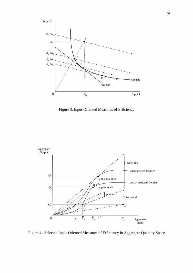
46

Figure 3. Input-Oriented Measures of Efficiency

Figure 4. Selected Input-Oriented Measures of Efficiency in Aggregate Quantity Space

A

Aggregate Output

Aggregate Input

0

B

itX *tX

E *tQ

itQ

technical

pure scale

pure mix

D

U

scale-mix

itXˆitX

unrestricted frontier

mix-restricted frontier

itX

itQ

residual mix

A

0

B

Input 1

U

R

2/itX

Input 2

2itx

2/itX

2/itX

2ˆ /itX

1itx

isoquant

isocost

47

Figure 5. Productivity Change in the Petroleum and Coal Products Sector: 1987-2008.

Figure 6. Output and Input Change in the Petroleum and Coal Products Sector: 1987-2008.

0.6

0.8

1

1.2

1.4

1.6

1.8

2

2.219

87

1989

1991

1993

1995

1997

1999

2001

2003

2005

2007

Fare‐Primont

Lowe

Geometric Young

Chained Hicks‐Moorst.

Chained Fisher

Chained Tornqvist

Fisher‐EKS

Tornqvist‐EKS

0

0.5

1

1.5

2

2.5

3

1987

1989

1991

1993

1995

1997

1999

2001

2003

2005

2007

∆Q

∆K

∆L

∆E

∆M

∆S

48

Figure 7. Productivity Change in Selected Sectors: 1987-2008.

Figure 8. Levels of Productivity and Efficiency in the Computer and Electronic Products

Sector: 1987-2008.

0

0.1

0.2

0.3

0.4

0.5

0.6

0.7

0.8

0.9

119

87

1989

1991

1993

1995

1997

1999

2001

2003

2005

2007

Food Beverage & Tobacco Products

Apparel & Leather & Applied Products

Petroleum & Coal Products 

Chemical Products 

Computer & Electronic Products 

0

0.1

0.2

0.3

0.4

0.5

0.6

0.7

0.8

0.9

1

1987

1989

1991

1993

1995

1997

1999

2001

2003

2005

2007

MFPMFP*MFPE = MFP/MFP* = ITE x ISMEITEISMEMFPMFP*MFPE = MFP/MFP* = ITE x ISME

49

Figure 9. Levels of Productivity and Efficiency in the Apparel and Leather and Applied Products Sector: 1987-2008.

Figure 10. Estimated (Unrestricted) Production Frontiers: 1987 and 2008.

0

0.1

0.2

0.3

0.4

0.5

0.6

0.7

0.8

0.9

119

87

1989

1991

1993

1995

1997

1999

2001

2003

2005

2007

MFP

MFP*

MFPE = MFP/MFP* = ITE x ISME

ITE

ISME

0 0.5 1 1.5 2 2.5 3

1987

2008

2.5

2

1.5

1

Q

x

1993

2001

337  Furniture

321  Wood

311, 312 Food

315, 316 Apparel313, 314 Textiles

335 Electrical

334 Computers

311, 312 Food

50

REFERENCES

Allen, R., A. Athanassopoulos, R. G. Dyson and E. Thanassoulis (1997). "Weight restrictions

and value judgements in Data Envelopment Analysis: Evolution, development and

future directions." Annals of Operations Research 73: 13-34.

Atkinson, S. E., C. Cornwell and O. Honerkamp (2003). "Measuring and Decomposing

Productivity Change: Stochastic Distance Function Estimation Versus Data

Envelopment Analysis." Journal of Business and Economic Statistics 21(2): 284-294.

Balk, B. M. (1998). Industrial Price, Quantity, and Productivity Indices: The Micro-

Economic Theory and an Application. Boston, Kluwer Academic Publishers.

Balk, B. M. (2008). Price and Quantity Index Numbers: Models for Measuring Aggregate

Change and Difference. New York, Cambridge University Press.

Bjurek, H. (1996). "The Malmquist Total Factor Productivity Index." Scandinavian Journal

of Economics 98(2): 303-313.

BLS (2010). "Manufacturing Sector and NIPA-level Manufacturing Industries KLEMS

Multifactor Productivity Tables by Industry." United States Department of Labor.

http://www.bls.gov/mfp/mprdload.htm (accessed December 2, 2010).

Briec, W. and K. Kerstens (2004). "A Luenberger-Hicks-Moorsteen Productivity Indicator:

Its Relation to the Hicks-Moorsteen Productivity Index and the Luenberger

Productivity Indicator." Economic Theory 23(4): 925-939.

Briec, W. and K. Kerstens (2011). "The Hicks-Moorsteen Productivity Index Satisfies the

Determinateness Axiom." Manchester School 79(4): 765-775.

Caves, D. W., L. R. Christensen and W. E. Diewert (1982a). "The Economic Theory of Index

Numbers and the Measurement of Input, Output, and Productivity." Econometrica

50(6): 1393-1414.

51

Caves, D. W., L. R. Christensen and W. E. Diewert (1982b). "Multilateral Comparisons of

Output, Input, and Productivity Using Superlative Index Numbers." The Economic

Journal 92(365): 73-86.

Coelli, T. J., D. S. P. Rao, C. J. O'Donnell and G. E. Battese (2005). An Introduction to

Efficiency and Productivity Analysis. New York, Springer.

Dean, E. R., M. J. Harper and M. S. Sherwood (1998). "Productivity Measurement With

Changing-Weight Indices of Outputs and Inputs". Industry Productivity: International

Comparison and Measurement Issues: OECD Proceedings: 183-215.

Diewert, W. E. (1992). "Fisher Ideal Output, Input, and Productivity Indexes Revisited."

Journal of Productivity Analysis 3: 211-248.

Edgeworth, F. Y. (1925). Papers Relating to Political Economy. Volume I. London,

Macmillan.

Eichhorn, W. (1976). "Fisher's Tests Revisited." Econometrica 44(2): 247-256.

Elteto, O. and P. Koves (1964). "On a Problem of Index Number Computation Relating to

International Comparison." Statisztikai Szemle 42: 507-518.

Färe, R. and S. Grosskopf (1990). "A Distance Function Approach To Price Efficiency."

Journal of Public Economics 43(1990): 123-126.

Färe, R., S. Grosskopf, M. Norris and Z. Zhang (1994). "Productivity Growth, Technical

Progress, and Efficiency Change in Industrialized Countries." American Economic

Review 84(1): 66-83.

Färe, R., S. Grosskopf and P. Roos (1996). "On Two Definitions of Productivity." Economics

Letters 55: 169-274.

Färe, R. and D. Primont (1995). Multi-output Production and Duality: Theory and

Applications. Boston, Kluwer Academic Publishers.

52

Farrell, M. J. (1957). "The Measurement of Productive Efficiency." Journal of the Royal

Statistical Society, Series A (General) 120(3): 253-290.

Fisher, I. (1922). The Making of Index Numbers. Boston, Houghton Mifflin.

Fox, K. J. (2003). "An Economic Justification for the EKS Multilateral Index." Review of

Income and Wealth 49(3): 407-413.

Grifell-Tatjé, E. and C. A. K. Lovell (1995). "A Note on the Malmquist Productivity Index."

Economics Letters 47(2): 169-175.

Grosskopf, S., D. Margaritis and V. Valdmanis (1995). "Estimating output substitutability of

hospital services: A distance function approach." European Journal of Operational

Research 80(1995): 575-587.

Gullickson, W. (1995). "Measurement of productivity growth in U.S. manufacturing."

Monthly Labor Review 118(7): 13-27.

Hicks, J. R. (1961). "Measurement of Capital in Relation to the Measurement of Other

Economic Aggregates" in Lutz, F. A. and D. C. Hague (eds.) The Theory of Capital.

London, Macmillan.

IMF (2004). Producer Price Index Manual: Theory and Practice. Washington, D.C.,

published for the ILO, IMF, OECD, UNECE and World Bank by the International

Monetary Fund.

Jorgenson, D. W. and Z. Griliches (1967). "The Explanation of Productivity Change." The

Review of Economic Studies 34(3): 249-283.

Lovell, C. A. K. (2003). "The Decomposition of Malmquist Productivity Indexes." Journal of

Productivity Analysis 20: 437-458.

Lowe, J. (1823). The Present State of England in Regard to Agriculture, Trade and Finance.

London, Longman, Hurst, Rees, Orme and Brown.

53

Marshall, A. (1887). "Remedies for Fluctuations of General Prices." Contemporary Review

51: 355-375. .

Moorsteen, R. H. (1961). "On Measuring Productive Potential and Relative Efficiency." The

Quarterly Journal of Economics 75(3): 151-167.

Nemoto, J. and M. Goto (2005). "Productivity, efficiency, scale economies and technical

change: A new decommposition analysis of TFP applied to the Japanese prefectures."

Journal of the Japanese and International Economies 19(4): 617-634.

Nishimizu, M. and J. M. Page (1982). "Total Factor Productivity Growth, Technological

Progress and Technical Efficiency Change: Dimensions of Productivity Change in

Yugoslavia, 1965-1978." The Economic Journal 92(368): 920-936.

O'Donnell, C. J. (2008). "An Aggregate Quantity-Price Framework for Measuring and

Decomposing Productivity and Profitability Change." Centre for Efficiency and

Productivity Analysis Working Papers WP07/2008. University of Queensland.

http://www.uq.edu.au/economics/cepa/docs/WP/WP072008.pdf.

O'Donnell, C. J. (2010a). "Measuring and Decomposing Agricultural Productivity and

Profitability Change." Australian Journal of Agricultural and Resource Economics

54(4): 527-560.

O'Donnell, C. J. (2010b). "Nonparametric Estimates of the Components of Productivity and

Profitability Change in U.S. Agriculture." Centre for Efficiency and Productivity

Analysis Working Papers WP02/2010. University of Queensland.

http://www.uq.edu.au/economics/cepa/docs/WP/WP022010.pdf.

O'Donnell, C. J. (2011). "Econometric Estimation of Distance Functions and Associated

Measures of Productivity and Efficiency Change." Centre for Efficiency and

Productivity Analysis Working Papers WP01/2011. University of Queensland.

http://www.uq.edu.au/economics/cepa/docs/WP/WP012011.pdf.

54

O'Donnell, C. J. and K. Nguyen (2011). "An Econometric Approach to Estimating Support

Prices and Measures of Productivity Change in Public Hospitals." Centre for

Efficiency and Productivity Analysis Working Papers WP03/2011. University of

Queensland. http://www.uq.edu.au/economics/cepa/docs/WP/WP032011.pdf.

Pilat, D. and D. S. P. Rao (1996). "Multilateral Comparisons of Output, Productivity and

Purchasing Power Parities in Manufacturing." Review of Income and Wealth 42(2):

113-130.

Shephard, R. W. (1953). Cost and Production Functions. Princeton, Princeton University

Press.

Szulc, B. J. (1964). "Indices for Multi-regional Comparisons." Prezeglad Statystyczny

(Statistical Review) 3: 239-254.

Timmer, M. P., M. O'Mahony and B. van Ark (2007). "Growth and productivity accounts

from EU KLEMS: An overview." National Institute Economic Review 200(1): 64-78.