The underground economy in the Czech Republic: dynamic ...
39
The underground economy in the Czech Republic: dynamic general equilibrium modeling and policy analysis Martial Dupaigne * 27th February 2001 Abstract This paper studies the issue of tax evasion in the context of the un- derground economy. A dynamic general equilibrium model is built where individual households and entrepreneurs decide rationally whether to go underground and under-report their earnings. These behaviors affect tax revenues, which are used to finance productive public services. This model is applied to the Czech Republic, because transition economies face admittedly high public investment needs but also large problems in the tax collection process. When deep parameters are calibrated on this econ- omy, the predicted relative size of the underground economy lies around 15% of measured GDP in the long-run, which is in the upper band of current estimates for this country. In this framework, we first evaluate how the design of the tax system – as described by tax rates, tax mix between direct and indirect taxes and the efficiency of fraud detection – affects the relative size of the underground economy, measured and total output and aggregate welfare in the long-run. Our second experiment is to identify the effects of an underground economy on the transition process, by comparing our model economy to a benchmark where agents have no access to an underground technology. We find that the underground economy significantly decreases the speed of adjustment. The model also predicts that the relative size of the un- derground economy should rise in the beginning of the transition process, and then eventually return to its long-run level. 1 Introduction Underground activities are as widely spread around the world as taxes are. Wherever taxes are collected, tax non-compliance is a crucial issue policymak- ers. This is specially the case in developing economies, where very few public * CEPREMAP, 142 rue du Chevaleret, F-75013 Paris, and EUREQua, Universit´ e de Paris I. This research is undertaken with support from the European Union’s Phare ACE Program, Contract P97-8226-R. The content of the publication is the sole responsibility of the author and it in no way represents the view of the Commission or its services. The author owes much to P-Y H´ enin for numerous discussions on the topic and thanks Christophe Hurlin for his input on the subject. 1
Transcript of The underground economy in the Czech Republic: dynamic ...

The underground economy in the Czech Republic:
dynamic general equilibrium modeling and policy
analysis
Martial Dupaigne ∗
27th February 2001
AbstractThis paper studies the issue of tax evasion in the context of the un-
derground economy. A dynamic general equilibrium model is built whereindividual households and entrepreneurs decide rationally whether to gounderground and under-report their earnings. These behaviors affect taxrevenues, which are used to finance productive public services.
This model is applied to the Czech Republic, because transition economiesface admittedly high public investment needs but also large problems in thetax collection process. When deep parameters are calibrated on this econ-omy, the predicted relative size of the underground economy lies around15% of measured GDP in the long-run, which is in the upper band ofcurrent estimates for this country.
In this framework, we first evaluate how the design of the tax system –as described by tax rates, tax mix between direct and indirect taxes and theefficiency of fraud detection – affects the relative size of the undergroundeconomy, measured and total output and aggregate welfare in the long-run.
Our second experiment is to identify the effects of an undergroundeconomy on the transition process, by comparing our model economy toa benchmark where agents have no access to an underground technology.We find that the underground economy significantly decreases the speedof adjustment. The model also predicts that the relative size of the un-derground economy should rise in the beginning of the transition process,and then eventually return to its long-run level.
1 Introduction
Underground activities are as widely spread around the world as taxes are.Wherever taxes are collected, tax non-compliance is a crucial issue policymak-ers. This is specially the case in developing economies, where very few public
∗CEPREMAP, 142 rue du Chevaleret, F-75013 Paris, and EUREQua, Universite de ParisI. This research is undertaken with support from the European Union’s Phare ACE Program,Contract P97-8226-R. The content of the publication is the sole responsibility of the authorand it in no way represents the view of the Commission or its services. The author owes muchto P-Y Henin for numerous discussions on the topic and thanks Christophe Hurlin for hisinput on the subject.
1

services and infrastructures are available. In these countries, the marginal re-turn to public capital is very high and under-reported tax-base is likely to betaken away from its socially most valuable uses.
Central and Eastern European economies experience different problems. Af-ter the transition from centrally planned to market economies, the quality ofpublicly provided services and infrastructures may matter more than their quan-
tity. But more specifically, tax collection seems really difficult in these countriesused to off–market transactions and direct state controls over many economicprocesses. Countries in transition are therefore confronted with the potentialvicious circle of large underground economies: inefficient tax collection calls forincreases in average tax rates, which incite businesses to go underground andreduce the fiscal base, and so on.
The literature dealing with the underground economy is now substantial.Basically, much macroeconomic work consists in various attempts to measurethe relative size of hidden output relative to reported output (see for examplethe ‘Controversy: on the use of the “hidden economy” estimates’, EconomicJournal, june 1999, vol. 109, or papers cited in Schneider and Enste [2000]).Beside econometric methodological issues, Thomas [1999] among others hasquestioned the relevance of these studies to guide economic policy.
Loayza [1996] provides an interesting theoretical macroeconomic model link-ing the size of the underground economy to growth, through the accumulationof public capital. Asea [1996] however points the lack of microeconomic foun-dations of the labor share devoted to both sectors.
A number of microeconomic studies of the underground economy addressthese issues. On the theoretical side, a specific literature has grown up from theearly tax evasion model of Allingham and Sandmo [1972]. Sandmo [1981], Jung,Snow and Trandel [1994] or Trandel and Snow [1999] analyze the individualdecision to participate to the underground economy as part of the gamble agentsplay when they under-report their income. On the empirical side, Lemieux,Fortin and Frechette [1994] and Fortin, Lacroix and Montmarquette [2000] usesurvey results to quantify the effects of economic policies.
In this paper, we try to connect these distinct strands of literature and tobuild a micro-founded dynamic general equilibrium model able to evaluate dif-ferent economic policies. As such, it follows Fortin, Marceau and Savard [1997]and Piggott and Whalley [1998] who have developed applied general equilib-rium models, respectively calibrated on Cameroon and Canada. Beside numer-ous specifications differences, the main originality of our model with respect totheirs lies in its explicit dynamic dimension. In addition to long–run experi-
2

ments, this dimension allows to carry on transition-specific exercises focusingon the accumulation of private and public capital.
The main results we obtain are the following. First, individual labor sup-ply tradeoffs give rise to a Laffer curve, i.e. a non-monotonic relation between(marginal) tax rates and fiscal revenues. This non-monotonicity is purely dueto this form of tax evasion, as can be seen from a control experiment in an un-derground activity–free economy. We also show that optimal public investmentrules are affected. Second, the design of the tax system, as witnessed by thefiscal mix between direct and indirect taxes, affects the relative size of the un-derground economy. Intuitively, this should be the case if underground activitydoes not escape sales taxes (VAT) as easily as income taxes. Third, the exis-tence of the underground economy slows down the transition currently takenplace in transition economies, as exemplified by the Czech Republic. Hence thelong–run (in)efficiency of informal sectors is not the only thing that matter.
2 A dynamic general equilibrium model of the un-derground economy
2.1 Tax evasion and labor supply behavior
Early static models of tax evasion, following Allingham and Sandmo [1972]or Yitzhaki [1974], have studied the under-reporting of a given level of actualincome. Agents play a gamble in order to evade part of their true tax liability, atthe cost of a penalty if they get detected. Sandmo [1981] has shifted attentiontowards labor supply. He considers an unofficial sector when income under-reporting is possible, next to the official sector where it is not (for examplebecause both employers and employees declare income). According to this view,the only motivation driving agents to participate to the underground part ofthe economy is to evade existing taxes and regulations, including income tax,regulations, license fees, red tape and so on.
Labor supply issues justify a dynamic setup as soon as wealth effects exertinfluence on employment rates (or average work length) and on participationchoices to either of the two sectors. Dynamic extensions of existing static modelscannot however be performed in a straightforward manner in a representativeagent framework. In fact, labor supply and consumption/savings decision areindividually taken ex ante, before the tax agency tries to detect frauds, on thebasis of expected utility - a weighted sum of the utility level if under-reportingis not detected and of the utility level is fraud is known and penalties are
3

incurred. Ex post wealth would differ though,1 between households who didparticipate into the underground economy but did not get caught and thosewho also participate in this unofficial sector and had to pay the associatedpenalties.2
In this paper, we will follow Kesselman [1989], Fortin et al. [1997] and Fortinet al. [2000] and assume that agents participating to the underground sector canavoid detection (with probability 1),3 through a costly process of camouflage.As a consequence, participation choices to the informal sector do not dependupon preferences regarding risk any longer. Only earnings differential matter:an individual household rationally works in the unregistered activity as long asits marginal unofficial income, net from concealment costs, exceeds the after-taxhourly wage rate.
Next we describe what are the earnings gained in both sectors.
2.2 Technology and incomes in the registered and undergroundactivities
The registered activity
Firms operating in the registered part of the economy have access to a constantreturns-to-scale technology, with regard to private inputs – per-capita labor Ht
and capital stock Kt. We assume that the public sector has a (positive) externaleffect on the output of these private firms. Such productive public services canbe interpreted as education facilities, transport infrastructures or simply theaccess to a legal system enforcing property rights and private contracts.
The productive nature of public services is a required dimension to avoid thetrivial result that an underground sector is welfare-improving, since it decreasesthe tax-induced distortions.4 Here, an increase in the share of the undergroundeconomy decreases the overall tax burden, but also the amount of productivepublic expenditures. Following Loayza [1996], we consider that the size ofthe underground economy may exert a second negative effect, because publicservices are subject to congestions from the two types of activities, registered
1In such cases, it is commonly assumed in the representative agent literature that house-holds have access to an insurance device, so that the ex post wealth level remains constantbetween the two types of agents. See Rogerson [1988] for an illustration regarding the unem-ployment risk.
2P-Y Henin has pointed out an alternative way to get rid of this wealth heterogeneityproblem: if penalties on detected defrauding agents are payed in consumption goods once theagents have taken their savings as well as their consumption decisions, agents will only differin ex post utility levels.
3On the survey Fortin et al. [2000] ran in Quebec, only 1.2% of households effectivelyworking in the underground economy declare having been caught by the tax agency.
4Barro [1990] and Easterly [1993] elaborate on these points in endogenous growth frame-works.
4

and unregistered. At the difference of Loayza [1996] however, participationchoices of individuals are considered in this model.
The production function of the representative firm active in the registeredactivity writes:
Yt = F(Γt, Ht, Kt, Gt, Yt
)= ΓtH
α1t K1−α1
t
{Gt
(Yt+Yt)φ
}α2 (1)
with 0 < α1 < 1 and 0 < α2 < 1. Variables with the superscript ‘ ˜ ’ denotethose related to the unofficial sector. Since α2 > 0, the level of public servicesrelative to output that agents take as given, Gt
(Yt+Yt)φ, has a positive external
effect on the output of the registered activity. The parameter φ is used tocompare the prediction of the model when productive public services are subjectto congestion (φ > 0) and when they are not (φ = 0). Finally, Γt denotes anexogenous productivity term which will be used to model the catch-up of adeterministic trend γt
x.
The unregistered activity
As already mentioned, the unregistered activity has to be disguised in orderto avoid detection by tax agencies. The earnings which should be consideredwhen deciding to enroll in this unofficial activity are therefore the earningsnet of these decoy costs. We assume that the net output of the unregisteredactivity only depends on the quantity of labor used and exhibits decreasingreturns-to-scale:
Yt = B (η, t) Hσt , 0 < σ < 1. (2)
In this expression, the exogenous productivity term B (η, t) ≡ γtx b(η) is used
to scale the efficiency of the unregistered activity relatively to the official one.Due to decoy costs, it depends negatively on the enforcement effort of the taxagency η, which we assume to be an institutional parameter. It also evolvesover time, so that the average product of labor follows the same deterministictrend in both activities.
The underground activity does not benefit from the positive external effectof public expenditures because of its illegal status.
We give two arguments to justify that the underground activity does not useany capital input. The first one is that physical capital input would make theunderground activity visible, and therefore detectable. Alternatively, if theseactivities use capital input as well as labor, the net earnings function (2) requiresthat the costs of avoid detection also increases with Kt such that the marginalproduct of capital is exactly equal to the marginal costs of avoiding detectionwhen one more unit of capital is operated in the underground economy.
5

Our second argument is an empirical one. Using a survey in Quebec,Lemieux et al. [1994] find that the earnings in the underground activity area concave function of hours, whereas earnings in the official activity are linear,as it is the case when the hourly wage rate is constant. Hence, Lemieux et al.[1994] advocate the use of an earning function of the type considered here.5
Due to the decreasing returns-to-scale, the underground activities raise prof-its (even in equilibrium). We make the usual assumption that these profits willeventually benefit to the households. However, the households does not takethe level of profit as given when they determine the amount of time allocatedto the underground activity. In other words, the representative households isassumed, for simplicity of exposition, to act as a shareholder in the official ac-tivity but as an entrepreneur in the underground activity. But the decisionrules that we obtain under this assumption remain fully compatible with analternative market interpretation where any household simultaneously sells itslabor on the undeclared labor market, gets the unofficial wage, and finally buyslabor to run its unregistered activity, earning the profits.
This underground activity differs from household production because itsoutput can be, and is, sold on a market.
2.3 The financing of productive public services
The productive public services are financed through a proportional (distorting)tax hitting official incomes at rate T I and a linear consumption tax at rateTC . The income tax rate is the same for labor and capital income, but capitalincome gets a tax credit under the form of a depreciation allowance T IδKKt.
The existence of an unregistered activity raises the specific issue of tax onintermediate consumption. What is called a consumption tax is in fact a value–
added tax, because taxes payed on the goods used as intermediate consumptionin the production process of the registered activity are deductible. On the con-trary, the unregistered activity cannot take advantage of this tax exemption.As a consequence, the underground activity is partially and indirectly taxed.In the model, we assume that, in the underground activity, intermediate con-sumption represents a fixed proportion θ of output Yt. Hence, the fiscal revenueof this activity writes TCθYt.
Public expenditures are twofold. First, public investment Xt is accumulated5Piggott and Whalley [1998] use a similar function to describe the underground supply
and self-supply of services. In their calibrated exercise related to Canada in 194, they set theelasticity of this supply function to .6.
6

into a stock of public capital which depreciates at rate δG:
Gt = (1− δG)Gt−1 + Xt. (3)
For reasons that will become apparent in the calibration section, public expen-ditures also finance lump-sum transfers to households Tt in this model economy.A balanced-budget requirement writes:6
Xt + Tt = T I [wtHt + rtKt + πt]− T IδKKt + TCCt + TCθYt (4)
At every date t, expression (4) gives the amount of per-capita public in-vestment and transfers induced by the equilibrium on labor, capital, and goodmarkets.
2.4 Relative prices
As long as the same (composite) good is supplied by both activities, the after-tax relative price of one unit of good supplied by the regular activity to one unitof good supplied by the underground activity must be one. For that reason,we label in what follows Ct the aggregate flow of consumption regardless of theactivity that did produce the good consumed. This flow can be disentangled expost between the consumption of irregularly produced goods, which equal theproduction level Yt, and the consumption of regularly produced goods, Ct− Yt.
However, this ‘law of one price’ should prevail whether the good is usedfor consumption or for investment. But consumption is taxed, whereas invest-ment is not. Consequently, interior solutions on consumption and investment —outcomes where goods produced from both activities are simultaneously con-sumed and accumulated — are incompatible; either the output of the regularactivity is never consumed or the output of the underground activity is neveraccumulated. We retain the latter equilibrium.
2.5 The equilibrium
The economy is inhabited by a large number of identical infinitely-living house-holds. The population size is constant and normalized to unity. We distinguishvariables over which the household has control to their aggregate counterpartsby using lower-case and upper case letters respectively.
Given the tax rates T I and TC and public transfers Tt, the hourly wagerate in the official activity wt and the (gross) rental price of capital rt, thevalue of aggregate state variables st = (At, Bt) and its initial stock of physical
6This paper does not consider the issue of tax-financing vs debt-financing. In spite ofthe distortions induced by the tax system, we believe that we are ‘too’ close to Ricardianequivalence for that distinction to matter.
7

capital k0, every household chooses consumption plans ct and hours of workin the official ht and unofficial economy ht in order to maximize the expecteddiscounted value of utility, subject to sequences of budget constraints:
max{ct,ht,ht}
E0
{+∞∑t=0
βt U[ct, ht, ht
]}
s.t.
kt+1 ≤ (1− δK)kt + T IδKkt −(1 + TC
)ct
+(1− T I
)[wtht + rtkt + πt]
+ (1− θ)(1 + TC
)B(η, t)hγ
t + Tt
ct ≥ 0, t = 0, ...,+∞0 ≤ ht ≤ 1,
0 ≤ ht ≤ 1
given k0 ≥ 0.
The first-order conditions of the household’s program write:
∂U(·)∂ht
=1− T I
1 + TCwt
∂U(·)∂ct
(5)
∂U(·)∂ht
= (1− θ)σ Bt hσ−1t
∂U(·)∂ct
(6)
∂U(·)∂ct
= β Et
{[1 +
(1− T I
)(rt+1 − δK)
] ∂Ut+1
∂ct+1
}(7)
The following transversality condition holds:
limt→∞E0
{βt ∂U(·)
∂ctKt+1
}= 0. (8)
Given tax rates, wages and prices, the representative firm operating in theofficial activity chooses the per-capita quantities of labor Ht and capital Kt
that maximize its profit:
max{Ht,Kt}
πt = F(At, Ht, Kt, Gt, Ht
)− wtHt − rtKt
The first-order conditions of this optimization problem write:
∂F (·)∂Ht
= wt (9)
∂F (·)∂Kt
= rt (10)
A competitive equilibrium of this economy is a set of individual decisionsrules
{c (st, kt, Kt) , h (st, kt, Kt) , h (st, kt, Kt)
}, a set of aggregate decision rules{
C (st, Kt) , H (st, Kt) , H (st, Kt)}
and a set of price functions {w (st, Kt) , r (st, Kt)}such that:
8

i) the optimality conditions of the household’s program, (5) to (8), are satisfied,
ii) the optimality conditions of the firm’s program, (9) and (10), are satisfied,
iii) the balanced-budget rule (4) is verified,
iv) individual and aggregate decisions are consistent,
c (st, Kt, Kt) = C (st, Kt) ∀st ∀Kt
h (st, Kt, Kt) = H (st, Kt) ∀st ∀Kt
h (st, Kt, Kt) = H (st, Kt) ∀st ∀Kt
v) the good market, the capital market and the labor markets are cleared:
Ct + Kt+1 − (1− δK)Kt + Gt = F(At, Ht, Kt, Gt, Ht
)+ (1− θ)BtH
γt
kt = Kt
2.6 Calibration
Functional forms
We have already presented the production function of the registered and un-registered activity. We also consider a Cobb-Douglas utility function:
U[ct, ht, ht
]= a log (ct) + (1− a) log
(1− ht − ht
).
Parameter values
We set the value of structural parameters of this model based on a priori in-formation and to match some recent observations on Czech National Accounts.The parameters values are summarized in table 1.
Table 1: Calibration
TC T I γx α1 α2 δK δG σ θ a β
.25 .232 1.006 .58 .05 .03 .03 .65 .32 .401 .98
The proportional tax rate on consumption TC is set to 25%, which is theaverage share of indirect taxes in measured consumption over the 1993–1998sample. The tax rate on income T I includes direct taxes as well as social securitycontributions. They average 23.2% of measured income over the sample. Theshare of public investment to GDP is fixed to 6.4% (these number were takenform the OECD [2000] report). This means that public spending are 5 times as
9

large as public investment alone. We have modelled this discrepancy as a lump–sum transfer to household. The numbers we use imply a 30% transfer-to-GDPratio.
In the registered activity, the elasticity of output with respect to labor, α1,is equal to the share of labor income in output, which averages 58%. The valueretained for α2, the elasticity of public capital, is .05 (Hurlin [2000]). Sensitivityanalysis will be performed over this parameter value.
It is fairly uneasy to pin down a value for the growth factor of the Harrod-neutral technical progress. Because this is the only source of (deterministic)growth in this model, γx determines the long-run growth rate of output, con-sumption and capital. However, the observed per capita counterparts of thesevariables do not display balanced growth and constant growth rates. For ex-ample, over the sample 1993–1998, the annual growth rate of real per-capitaoutput averages 3%, with a peak of 6.5% from 1994 to 1995 and a throughof −2.8% from 1997 to 1998. We retain the value γx = 1.006, which imply aquarterly growth rate of .6%, slightly below the sample average but still abovethe usual calibrations for Western-European countries.
The depreciation rate of the private capital stock δK is equal to .03, asimplied by the average investment-capital ratio (given γx). Following Cooleyand Prescott [1995], the depreciation rate of the public capital stock is fixed tothe same value than that of private capital δG = δK .
The weight of consumption flows in the temporal utility function, a, ischosen such that H, the average share of the time endowment allocated toregistered labor, matches its empirical counterpart .33.7
In the underground activity, the elasticity of earnings with respect to under-ground labor σ is given the value .65, which is the point estimate obtained onQuebec data in Lemieux et al. [1994]. Of course, this value is subject to cautionand the robustness of our results is tested. A survey related to undergroundlabor supply is currently run is the Czech and Slovak republics as part of aPhare-ACE Program. The estimation procedure of Lemieux et al. [1994] willbe replicated on these data, once available.
The second parameter related to the underground activity is θ, the fixedcoefficient of intermediate consumption in the production function. Once again,no direct measure of this parameter is available. We however have two referencevalues. The first one is the share of intermediate consumption in market outputin the Czech Republic, which averages 72% over the sample. We expect thisfigure to be an upper bound, because the intermediate consumption is morecostly in the unregistered activity, due to the non-deductible consumption tax.
7In this computation, the time endowment is 70 hours a week.
10

Our second value is taken from the Quebec survey: according to these data,total income from the unregistered activity would be 27% higher that totalconsumption of underground goods. This discrepancy can be interpreted as theshare of underground output which is used to buy regular goods for intermediateconsumption motives. θ = .27 is our benchmark value in the quantitativeexercises undertaken in the following.
Finally, the psychological discount factor is set to .98, which implies a long-run real interest rate of 5%.
2.7 Sensitivity analysis
We have mentioned how uneasy it was to pin down values for the ‘deep’ param-eters of the underground activity, because of a lack of observation to rely upon.Sensitivity analysis shows how the model-predicted size of the undergroundeconomy varies along with α2, the elasticity of declared output with respectto public services, σ, the elasticity of labor in the undeclared activity, and θ,the proportion of underground intermediate consumption. These three valuesmatter for interior solutions of our problem since they appear in the arbitrageequation (11), which simply says that households modify their participationchoices until the marginal product revenues of both activities are equal:
1− T I
1 + TCα1 Γt Hα1−1
t K1−α1t
{Gt
(Yt + Yt)φ
}α2
= (1− θ)σ Bt Hσ−1t (11)
Two numbers are used to measure the size of the underground economy. Thefirst one is the ratio of the unregistered output Yt to the registered output Yt.This ratio is the theoretical counterpart of the relative size of the shadow econ-omy as percentage points of GDP, which is the most commonly used measurein empirical work (see Schneider and Enste [2000] for example). Our secondmeasure is the share of hours devoted to the unregistered activity Ht in totalhours worked Ht + Ht.
Congestion
Figures 1 and 2 respectively display the implied size of the underground econ-omy when public capital is subject to congestion and when it is not. The firstnoticeable feature is that congestion discourages participation into the officialactivity; for any value of the parameter studied, both measures of the size ofthe underground economy are greater when the productive services providedby public capital are subject to congestion (φ = 1) than when they are not
11

(φ = 0). However the quantitative discrepancy remains limited. For our bench-mark value (indicated with a grey line on any displayed panel), 17.8% of totalwork time is allocated to work in the unregistered activity, which productionamounts to 17.4% of registered output when public capital is subject to con-gestion. These numbers become respectively 16% and 15.4% when φ = 0.
Figure 1: Size of underground output — congestion case φ = 1
Share of undeclared output
0.02 0.04 0.06 0.08 0.1
0.15
0.16
0.17
0.18
0.19
α2
% o
f GN
P
Sensitivity to α2
0.5 0.6 0.7 0.8 0.9
0
0.1
0.2
σ
% o
f GN
P
Sensitivity to σ
0.2 0.4 0.60.15
0.16
0.17
0.18
0.19
θ
% o
f GN
P
Sensitivity to θ
Share of undeclared hours
0.02 0.04 0.06 0.08 0.1
0.16
0.18
0.2
α2
% o
f tot
al h
ours
Sensitivity to α2
0.5 0.6 0.7 0.8 0.9
0
0.05
0.1
0.15
0.2
σ
% o
f tot
al h
ours
Sensitivity to σ
0.2 0.4 0.6
0.1
0.15
0.2
θ
% o
f tot
al h
ours
Sensitivity to θ
The asymmetry explaining the positive effect of congestion on the under-ground economy lies in the access to the productive public services, which isstrictly restricted to the declared activity. This is clearly a very strong assump-tion, since many public infrastructures (roads, bridges, etc.) are open to alltypes of users. Should the unofficial activity have access to part of the publiccapital, congestion would decrease its productivity the same way as it affectsthe productivity of registered firms. Hence, congestion would not alter the rel-ative productivity of the registered and unregistered activity as much as it doesin the situation we consider. The comparison of numbers displayed in figures 1and 2 can therefore be interpreted as upper bounds of the effect of congestionof publicly provided productive services on our model economy.
12

Figure 2: Size of underground output — no congestion case φ = 0
Share of undeclared output
0.02 0.04 0.06 0.08 0.10.12
0.14
0.16
0.18
α2
% o
f GN
P
Sensitivity to α2
0.5 0.6 0.7 0.8 0.9
0
0.1
0.2
σ
% o
f GN
P
Sensitivity to σ
0.2 0.4 0.6
0.14
0.15
0.16
0.17
θ
% o
f GN
P
Sensitivity to θ
Share of undeclared hours
0.02 0.04 0.06 0.08 0.1
0.14
0.16
0.18
α2
% o
f tot
al h
ours
Sensitivity to α2
0.5 0.6 0.7 0.8 0.9
0
0.05
0.1
0.15
0.2
σ
% o
f tot
al h
ours
Sensitivity to σ
0.2 0.4 0.6
0.1
0.15
0.2
θ
% o
f tot
al h
ours
Sensitivity to θ
Parameters
α2, the elasticity of declared output with respect to public services, affectsthe size of the underground economy in a similar fashion to congestion. Thehigher α2, the higher the marginal product revenue in the registered activity,at no cost. Hence, a greater contribution of public capital to output inciteshouseholds to supply labor to the official activity, yielding a decrease in therelative size of the underground economy.
One might expect the effects of variation in σ, the elasticity of labor in theundeclared activity, to be reversed, since an increase in σ rises the reward toparticipate to the underground economy in (11). Figures 1 and 2 however showa large decrease in both measures of the size of the underground economy as σ
takes higher values.This counterintuitive finding is a by-product of the calibration procedure
described above: the weight of leisure in the static utility function a has beenset residually in order to match the average share of the time endowment al-located to registered work H. Hence, H, which is a control variable of themodel, must remain fixed throughout our experiments on σ. It implies thatthe marginal product of labor in the registered activity is determined indepen-
13

dently of σ. From equation (11), this means that the marginal productivity inthe unregistered activity has to remain constant when the elasticity of outputwith respect to labor varies. Due to decreasing returns, this implies that hoursworked in the unregistered activity H get lower as σ increases. When σ is 30%higher than in our benchmark calibration, the only value of H simultaneouslycompatible with the equality of marginal productivity and H = .33 is actuallyvery close to 0.
It must be noted however that fixing a from total hours of work H + H issimply not feasible, since we do not have yet any quantitative measure of timespent in undeclared activities in the Czech or Slovak Republics.
Finally, parameter θ describes which share of output in the unregisteredsector was bought from the regular sector to serve as intermediate consumption.It is also equal to one minus the share of undeclared output that effectivelyrewards underground workers. Straightforwardly from (11), the larger is θ, thesmaller the incentive to participate to the unregistered activity and its relativeshare.
3 Policy analysis
3.1 An increase in the efficiency of the fraud detection
The existence of an underground economy, as any form of tax evasion, raisesthe issue of the funding of the tax agency. Slemrod [1990] recalls the ‘claimof every IRS commissioner that each additional budget dollar allocated to theIRS will return on the order of ten dollars in increased revenues’. In the initialtax compliance literature, Slemrod and Yitzhaki [1987] stress that the socialmarginal benefit of strengthening enforcement, to which the social cost of extraenforcement should be compared, lies in ‘the value to risk-averse taxpayers ofpaying the required expected tax payment in a less risky manner, which occursbecause the higher probability of detection deters tax evasion gambling’.
Households in our model do not face the kind of uncertainty emphasized inthis literature, since they engage in a costly decoy activity that prevents theirunofficial work and income from being detected. Similarly, we do not modelthe detection process and the marginal cost of increasing tax compliance (bydecreasing the amount of time allocated to the unregistered sector).
We can however proxy an increase in the efficiency with which the taxagency would discover which agents work in the undeclared sector as a decreasein the parameter b (η) (which is equivalent to an increase in the enforcementeffort parameter η). This parameter describes the relative factor productivity
14

of the unregistered activity, once decoy costs are taken into account. If the taxagency becomes more efficient, these costs become larger, diminishing the netproduct of participating to the underground economy.
Figures 3 and 4 present the increase in welfare, measured in terms of long–run (declared) consumption, that would be achieved if b(η) was divided bytwo, for different values of parameters α2, σ and θ.8 For example, the leftpanel reads as follow: when α2 = .05, our benchmark value (grey line), therepresentative agent would be as well–off in the long–run if b(η) was half as largeas in the reference calibration or if official consumption increased permanentlyby nearly 6%. In other words, if total hours were to remain relatively constant,total consumption increase by around 5 percent forever when the undergroundactivity is less productive, which is a very large percentage.
Figure 3: An increase in the enforcement efficiency — congestion case φ = 1
0.02 0.04 0.06 0.08 0.1
5
5.5
6
6.5
7
α2%
of s
tead
y−st
ate
cons
umpt
ion Sensitivity to α
2
0.5 0.6 0.7 0.8 0.9
0
2
4
6
σ% o
f ste
ady−
stat
e co
nsum
ptio
n Sensitivity to σ
0.2 0.4 0.63
4
5
6
7
θ% o
f ste
ady−
stat
e co
nsum
ptio
n Sensitivity to θ
Figure 4: An increase in the enforcement efficiency — no congestion case φ = 0
0.02 0.04 0.06 0.08 0.14.5
5
5.5
6
α2%
of s
tead
y−st
ate
cons
umpt
ion Sensitivity to α
2
0.5 0.6 0.7 0.8 0.9
0
2
4
6
σ% o
f ste
ady−
stat
e co
nsum
ptio
n Sensitivity to σ
0.2 0.4 0.6
3
4
5
6
7
θ% o
f ste
ady−
stat
e co
nsum
ptio
n Sensitivity to θ
These numbers can be interpreted as measures of the welfare gain fromdiscouraging the underground economy through an apparently costless bettertax enforcement system. Note that from a social point of view however, any risein η – any decrease in b (η) – would be welfare decreasing if hours worked in
8We recall these notations: α2 denotes the elasticity of declared output with respect topublic services, σ is the elasticity of labor in the undeclared activity and θ is the proportionof underground intermediate consumption.
15

both activities remained unchanged. But the improved enforcement efficiencylowers the relative marginal revenue of the underground activity, yielding higherparticipation to the registered sector and lower participation to the undergroundone. Fiscal revenues and public investment therefore rise, and the external effectof public capital further stimulates registered output. Finally, the increase inregistered output does more than offset the decrease in underground outputin our experiments — the net variation of total output is around 3%. Still,this does not mean that the government should increase the resources allocatedto the tax agency, because we do not take the additional costs of improvedenforcement into account.
The gains vary along with some key parameter values. Our sensitivity anal-ysis concerns the parameter describing the production technology in the un-derground sector, σ and θ, as well as the elasticity of registered output withrespect to public capital α2.
• α2: The left panel of figure 3 shows that the welfare gains of an improve-ment of the enforcement system are increasing with α2. The higher α2,the more productive are public spending. The decrease in the share of theunderground economy illustrated in figure 1 raises fiscal revenue, publicinvestment, registered output and finally increases welfare.
• σ: The lower the returns to scale in the underground activity, the higherare the welfare gain from a more efficient enforcement system – the higherare the welfare costs due to the underground economy. Conversely, if un-registered activity has access to a very efficient production technology,discouraging households to participate to this sector is not welfare im-proving. Recall also that the size of the underground economy lowers asσ increases. At the limit case, an improvement of the enforcement systemdoes not make the representative better off, simply because virtually nounderground activity exists in the first place.
• θ: The share of unregistered production that really evades all kinds oftaxes is 1− θ. When θ is high, this share is low. Hence, the added fiscalrevenues from a policy that discourages underground activity are smaller.
3.2 Reforms of the tax system: the tax level
Given an institutional fraud detection efficiency,9 we now study the interac-tions between the tax system and the underground economy. Taxation and tax
9Given also institutional levels of corruption and bureaucratic requirements, which impor-tance is pointed out in Johnson, Kaufmann and Zoido-Lobaton [1998].
16

evasion form a vicious circle: high tax rates favor tax evasion, which erodesfiscal revenues and make higher tax rates necessary, etc. In this model economywith productive public capital, the following trade-off also arise: a decrease inthe tax burden will motivate agents to register in the official part of the econ-omy but will also decrease the availability of publicly provided services and theincitations to participate to the formal sector.
To pursue the quantitative evaluation of the relationship between the taxsystem and the size of the underground economy,10 we compute for differentincome and consumption tax rates the equilibrium resulting from rational be-havior of households and firms. We are then able to predict how these variationsin the tax level affect our model economy and the well-being of its ‘inhabitants’.In particular, total output and aggregate welfare, depicted in figures 5 and 7,sound useful indicators of the overall effect of these fiscal policies.
In the literature on optimal fiscal policy, a general result is that the welfare ofthe representative agent is maximized when the public investment rate is equalto the elasticity of output with respect to public capital, named α2 and equalto .05 in this paper. We can test the robustness of this result in an environmentwhere agents are able to evade part of their tax liability. Starting from low levelof taxes and public investment, does an increase in the tax rates remains welfareimproving if it leads more households to work in the unregistered activity? Toanswer this question, we keep the transfers-to-regular output ratio constantwhen tax rates vary.11 Therefore, the balanced-budget requirement translatesmodifications in the tax rates to the rate of public investment, as shown in thelower-right panel.
The income tax rate T I
Figure 5 shows that both measures of the relative size of the undergroundeconomy exhibit a U-shape when the income tax rate increases. We already haveemphasized the two opposite effects. An increase in the income tax rate distortsthe relative net products of working in the registered and unregistered activity.Provided that fiscal revenues increase, more public capital is accumulated and
10The issue of taxation when an underground economy exist has been studied in Jung et al.[1994] and Trandel and Snow [1999]. Sandmo [1990] and Kleven, Richter and Sørensen [2000]have considered another type of tax-escaping commodity, home produced services.
11We alternatively have kept the public investment-to-regular output ratio constant. Inthis case, the relative size of lump-sum transfers financed through distortive taxes is theadjustment variable that ensures the balance of budget. Results from this alternative exerciseare straightforward: the lower the tax rate, the higher the welfare. The less lump-sum transfersare financed with proportional taxes the better. In fact, aggregate welfare is in this casemaximized when tax rates are null, meaning that the (given) public investment rate is financedthrough negative lump-sum transfers, which is lump-sum taxation.
17

its external effect raises the productivity of labor in the registered firm. Due tothe decreasing returns to public services, the former effect dominates the latterfor large values of T I , that is for large public capital stocks. For an income taxrate twice as large as the current Czech income tax rate (vertical grey line),households spend in equilibrium half of their total working time participatingto the underground activity.
In the middle panel, we display total output and hours worked in twoeconomies, one with underground production (black dotted line) and one with-out (grey dotted line).12 In both cases, total output is non-monotonic anddisplays an inverse U-shape. As T I rises, more and more resources are devotedto the funding of public productive services, at decreasing returns to scale. Thefiscal wedge becomes larger, distorting the consumption-leisure decisions, aswitnessed by the decrease in total hours worked. When existing, these distor-tions increase the relative size of the underground economy, which is less efficientthan the registered one for high level of public capital: households work longerhours but total output is lower. Obviously, aggregate welfare would always behigher if agents had no access to the underground technology. This does notmean that the underground economy is not able to diminish fiscal distortions,but that these distortions are lower than the profitability of public investment.
The two lower panels handle the issue of the ‘optimal’ income tax rate. Theincome tax rate that maximizes the aggregate welfare in the steady state isequal to 19%, which is less than the current rate (vertical grey line). For thistax rate, the ratio of public investment to registered output13 attains 4.09% foran elasticity of declared output to public capital α2 equal to 5% (horizontal greyline).14 Hence, this experiment suggests that the existence of an undergroundproduction slightly biases downwards the optimal income tax rate in this modeleconomy.
The macroeconomic implications of fiscal evasion can be illustrated using therelation between fiscal revenues and the income tax rate, for a given consump-tion tax rate, which are displayed in figure 6. The left panel shows that botheconomies, with (model economy) or without access to the unofficial activity(benchmark economy), exhibit Laffer curves i.e. a non-monotonic relationshipbetween (marginal) income tax rates and fiscal revenues. However, the incometax rate beyond which any increase in T I actually induces losses in fiscal rev-
12Agents in both economies have the same preferences and endowment. Parameter valuesfor T I , T C , α1, α2 and a are the same in both experiments. In the benchmark economy, theonly technology agents have access to is production function (1).
13This ratio is greater than the ratio of public investment to total output.14The finding that the public investment to output ratio differs from the elasticity of public
capital is not an artifact from the grid used on T I .
18

Figure 5: Variations in the income tax rate when TC = 25%
Congestion case φ = 1
0.15 0.2 0.25 0.3 0.350.15
0.2
0.25
0.3
Share of unregistered output
0.15 0.2 0.25 0.3 0.35
0.15
0.2
0.25
0.3
Share of unregistered hours
0.15 0.2 0.25 0.3 0.351.3
1.4
1.5
1.6
1.7Total output
0.15 0.2 0.25 0.3 0.35
0.34
0.36
0.38
0.4
0.42
Total hours
0.15 0.2 0.25 0.3 0.35−14
−12
−10
−8
TI
Aggregate welfare
w/o unofficial activityw/ unofficial activity
0.15 0.2 0.25 0.3 0.35
0.05
0.1
0.15
TI
Rate of public investment
No congestion case φ = 0
0.15 0.2 0.25 0.3 0.35
0.15
0.2
0.25
Share of unregistered output
0.15 0.2 0.25 0.3 0.35
0.15
0.2
0.25
Share of unregistered hours
0.15 0.2 0.25 0.3 0.35
1.4
1.5
1.6
1.7
Total output
0.15 0.2 0.25 0.3 0.35
0.34
0.36
0.38
0.4
0.42
Total hours
0.15 0.2 0.25 0.3 0.35
−12
−10
−8
−6
TI
Aggregate welfare
w/o unofficial activityw/ unofficial activity
0.15 0.2 0.25 0.3 0.35
0.05
0.1
0.15
TI
Rate of public investment
19

enues is very different in the two considered specification. In the benchmarkeconomy, this rate is below 40% which might not seem a large number. Butwhen fiscal evasion through underground production occurs, the upper limiton the income tax rate is as low as 25%. It means that at the current rate, adecrease in the fiscal base would more than offset any rise of income the taxrate.
The right panel shows that the same qualitative results hold when the shareof public transfers to measured output, Tt
Yt, is held constant. As compared to
the previous situation, added fiscal revenues now finance public capital accumu-lation. Therefore, output of the registered sector continues to grow for highervalues of T I , and so does the fiscal base. Fiscal distortions exceed productivitygains when the income tax rate exceeds 50%. In the model economy, the Laffercurve is also shifted to the right: public capital accumulation raises the relativemarginal product of the official activity, and therefore make underground workless profitable, ceteris paribus.
Figure 6: The Laffer curve — Variations in the income tax rate
Congestion case φ = 1
0.1 0.2 0.3 0.4 0.5 0.60.3
0.35
0.4
0.45
0.5
0.55
0.6
TI
fisca
l rev
enue
s
Constant rate of public investment
w/o unofficial activityw/ unofficial activity
0.2 0.3 0.4 0.5 0.60.3
0.4
0.5
0.6
0.7
TI
fisca
l rev
enue
s
Constant rate of public transfers
w/o unofficial activityw/ unofficial activity
No congestion case φ = 0
0.1 0.2 0.3 0.4 0.5 0.60.3
0.35
0.4
0.45
0.5
0.55
0.6
TI
fisca
l rev
enue
s
Constant rate of public investment
w/o unofficial activityw/ unofficial activity
0.2 0.3 0.4 0.5 0.60.3
0.4
0.5
0.6
0.7
TI
fisca
l rev
enue
s
Constant rate of public transfers
w/o unofficial activityw/ unofficial activity
The consumption tax rate TC
Figure 7 concerns variations in the consumption tax rate TC . A rise in the con-sumption tax rate has the same qualitative effect on the underground economythan the rise in the income tax rate. However, we find in this model that both
20

indicators of the size of the underground economy respond much less to varia-tions in TC than to variations in T I . Part of the explanation would be that theunregistered activity escapes less to the consumption tax than to the incometax, because intermediate consumption of the unregistered activity cannot callfor a tax exemption.
The other difference between the response to variations in income tax rateslies in the nature of distorted choice. Both taxes distorts the consumption–leisure decisions, since they diminish the amount of goods that can be boughtwith the product of a marginal hour of work. But the consumption tax alsoputs a wedge between the additional work time required to consume a marginalunit of good15 and the additional work time required to invest in a marginalunit of good. This means that the consumption tax favors investment and ahigh level of private capital, yielding greater levels of registered output, rela-tive to consumption. Investment brings no demand to the unregistered firms,explaining that their output grows much more slowly with TC than with T I .
The consumption tax rate that maximizes steady-state aggregate welfare,24.5%, is close to the current rate. Contrary to the experiment on the incometax rate, the share of public investment in declared output for this value of TC
is 6.12%, above the elasticity of public capital α2. Hence, the optimal level ofconsumption tax rate appears to be higher when part of the production avoidstaxation.
The relation between fiscal revenues and the consumption tax rate TC ,the income tax rate being fixed, is displayed in figure 8. Conversely to theprevious experiment, it does not display a hump when agents do not haveaccess to the underground activity: increasing the consumption tax rate alwayspay in the benchmark economy. We have however seen that participation tothe underground sector increases with TC for such levels of taxation. Hence, aLaffer curve also occurs with respect to the consumption tax rate in our modeleconomy. The peak is attained for very large values of TC though: around 50%when the share of public investment in measured output is held constant (leftpanels) and nearly 80% when it varies with fiscal revenues, the share of publictransfers being fixed.
We should now discuss the assumption that output from both activities areperfect substitutes as consumption goods — recall that they are not when usedas intermediate consumption or public investment. As mentioned in section2.4, this implies the equality of after-tax prices of one unit of output from the
15Regardless of the activity that did produce that marginal unit of good. Remember thatin equilibrium, after-tax prices are the same.
21

Figure 7: Variations in the consumption tax rate when T I = 23.2%
Congestion case φ = 1
0.2 0.25 0.3 0.35
0.16
0.18
0.2
0.22
Share of unregistered output
0.2 0.25 0.3 0.350.16
0.18
0.2
0.22Share of unregistered hours
0.2 0.25 0.3 0.35
1.3
1.4
1.5
1.6
1.7
Total output
0.2 0.25 0.3 0.35
0.36
0.38
0.4
0.42
Total hours
0.2 0.25 0.3 0.35
−11
−10
−9
−8
TC
Aggregate welfare
w/o unofficial activityw/ unofficial activity
0.2 0.25 0.3 0.35
0.020.040.060.08
0.10.120.14
TC
Rate of public investment
No congestion case φ = 0
0.2 0.25 0.3 0.35
0.14
0.16
0.18
0.2
Share of unregistered output
0.2 0.25 0.3 0.35
0.16
0.18
0.2
Share of unregistered hours
0.2 0.25 0.3 0.35
1.4
1.6
1.8
Total output
0.2 0.25 0.3 0.35
0.36
0.38
0.4
0.42
Total hours
0.2 0.25 0.3 0.35
−10
−9
−8
−7
TC
Aggregate welfare
w/o unofficial activityw/ unofficial activity
0.2 0.25 0.3 0.35
0.020.040.060.08
0.10.120.14
TC
Rate of public investment
22

Figure 8: The Laffer curve — Variations in the consumption tax rate
Congestion case φ = 1
0.2 0.4 0.6 0.8
0.4
0.5
0.6
0.7
0.8
0.9
1
TC
fisca
l rev
enue
s
Constant rate of public investment
w/o unofficial activityw/ unofficial activity
0.2 0.4 0.6 0.8
0.4
0.6
0.8
1
TC
fisca
l rev
enue
s
Constant rate of public transfers
w/o unofficial activityw/ unofficial activity
No congestion case φ = 0
0.2 0.4 0.6 0.80.4
0.5
0.6
0.7
0.8
0.9
1
TC
fisca
l rev
enue
s
Constant rate of public investment
w/o unofficial activityw/ unofficial activity
0.2 0.4 0.6 0.8
0.4
0.6
0.8
1
TC
fisca
l rev
enue
s
Constant rate of public transfers
w/o unofficial activityw/ unofficial activity
registered activity and one unit of output from the unregistered activity. Hence,the consumption tax does not distort the relative price between these two typesof goods. It would not either affect labor allocation if unregistered output didfully escape taxation (if θ were equal to 0). In this case, it would only affectthe consumption-leisure trade-off.
If both type of output were imperfect substitutes for consumption, anyincrease in the consumption tax rate would increase the after-tax relative priceof the official good in terms of unofficial good. Similarly, the (real) net rewardfor one hour spent working in the unregistered activity would rise relatively tothe reward in the registered activity. Underground labor supply should thereforeshift up.
3.3 Reforms of the tax system: the tax mix
The previous analysis suggests that the income and consumption tax have dif-ferent quantitative effects in an economy with an underground sector. FollowingCaragata and Giles [2000], we investigate if the repartition of total tax revenuesbetween the two type of taxes matter. Specifically, we change the steady-stateshare of total tax revenues brought by the income tax keeping total tax revenues
as a share of registered output,T I(Y−δkK)+T C(C+θY )
Y , constant.In this exercise and in contrast with the two previous one, neither total pub-
lic spending nor public investment vary, when expressed in terms of declared
23

Figure 9: Variations in the tax mix
Congestion case φ = 1
0 0.2 0.4 0.6 0.8 1
0.1
0.15
0.2
0.25
0.3
0.35
0.4
weight of the income tax
Share of unregistered output
0 0.2 0.4 0.6 0.8 1
0.1
0.15
0.2
0.25
0.3
0.35
weight of the income tax
Share of unregistered hours
0 0.2 0.4 0.6 0.8 1
1.2
1.4
1.6
1.8
2
weight of the income tax
Total output
w/o unofficial activityw/ unofficial activity
0 0.2 0.4 0.6 0.8 1
−10
−5
0
5
weight of the income tax
Aggregate welfare
w/o unofficial activityw/ unofficial activity
No congestion case φ = 0
0 0.2 0.4 0.6 0.8 1
0.1
0.15
0.2
0.25
0.3
0.35
0.4
weight of the income tax
Share of unregistered output
0 0.2 0.4 0.6 0.8 1
0.1
0.15
0.2
0.25
0.3
0.35
weight of the income tax
Share of unregistered hours
0 0.2 0.4 0.6 0.8 1
1.2
1.4
1.6
1.8
2
weight of the income tax
Total output
w/o unofficial activityw/ unofficial activity
0 0.2 0.4 0.6 0.8 1
−10
−5
0
5
weight of the income tax
Aggregate welfare
w/o unofficial activityw/ unofficial activity
24

output. What is affected by this policy is the relative distortions caused by theincome and consumption tax, for a given amount of fiscal revenue. Figure 9shows that an income tax is more distorting and less efficient than a consump-tion tax in our model economy with underground production as well as in thebenchmark one.
The policy recommendation one could draw from this representative agentmodel would be to modify the structure of the tax system to enlarge the shareof fiscal revenue raised from the consumption tax. The desirability of this policyis however heavily subject to caution once redistribution issues are considered.It is widely believed that indirect taxation, such as a consumption tax, areregressive because wealthy people save a greater portion of their income thando low income households. For this reason, reducing the weight of the incometax in total fiscal revenues would shift part of the tax burden from rich to poorhouseholds, and may sacrifice too much equity on efficiency grounds.16
4 The underground economy along the transition
4.1 Transitional dynamics
Central and eastern european countries are still in a transition stage. Al-though they have shifted from centrally-planned economies to market-orientedeconomies, it remains hard to presume that they have attained their long-runbalanced growth path. On the contrary, these countries might rather be consid-ered as still converging to this long-run situation from a lower level of economicdevelopment.
Three kinds of initial conditions matter in the model described in the firstsection: the level of private and public physical capital, and the factor produc-tivity level. We successively study the transitional dynamics from these threedimensions.17
A low quantity of private physical capital
The first analysis we conduct is the transitional dynamics from a low initialcondition regarding the physical capital stock. In this case, the transition pathdescribes the accumulation process and its effect on both the official and unof-ficial sector. This exercise is similar in spirit to those undertaken in Christiano
16Piggott and Whalley [1998] present a reverse argument. According to them, broadeningthe VAT base induces a rise in underground production, which is undertaken by the poor andsold to the rich.
17It should be noted that these analysis could not be undertaken in partial equilibriumframeworks, since they involve modifications in relative prices after changes in the economicenvironment, taking into account decisions of both firms and households.
25

[1989], King and Rebelo [1993] or Canova and Ravn [2000].Figure 10 reports the evolution of output and hours, expressed as percentage
deviation from their long–run levels, when the economy starts with a privatecapital stock 1% below its steady–state level. As we did in our study of alter-native fiscal policy, we also display the path of a benchmark economy where noproduction is undeclared (grey lines).
Unsurprisingly, the upper-left and upper-right panels of figure 10 show that,in this model, both measures of the share of the underground economy aretemporarily large when not enough private capital is available. As the arbitragecondition (11) makes clear, the low level of private capital translates in a lower-than-average productivity of labor in the registered activity, which distorts theparticipation trade-off in favor of the unregistered activity.
The initial levels of output in both economies are low (middle-left panel),witnessing the lack of capital in the registered activity and despite a wealtheffect — total hours worked by households are transitory high (middle-rightpanel), as agents wish to accumulate private capital. The initial ‘drop’ in outputin the benchmark economy grey line) exceeds that of the model economy (blackline), because no labor-reallocation between the registered and unregisteredactivity can take place in the former. Because the lack of private capital doesstrike output harder when no underground technology is available, short–rungains exist to let an unregistered production occur.
However, it takes less than five years for the total output to become largerin the benchmark economy than in the model economy. At this stage, therelative deviation of total output has been reduced by a half in the benchmarksimulation. This speed of adjustment is consistent with the evidences in Kingand Rebelo [1993]. With access to an underground technology, the half-life ofoutput becomes longer than 15 years. These figures suggest that the existenceof an underground economy contributes to slow the transitional dynamic ofthis economy, by depriving the government to its ability to finance productivepublic capital and to stimulate the productivity of private factors.
The accumulation dynamics are displayed in the lower-left panel. In termsof private capital, it takes more than five years to fill half of the gap betweenthe initial conditions and the balanced–growth path. Finally, the lower-rightpanel shows that fiscal revenues have decreased during the transitional phase,due to low registered output and high fiscal evasion. After about ten years, thestock of public capital is nearly 1% below its initial level in the model economy,as compared to .5% in the benchmark.
As just emphasized, the gains from an existing underground sector areshortly-lived. In terms of aggregate welfare, the short–run gains are also quite
26
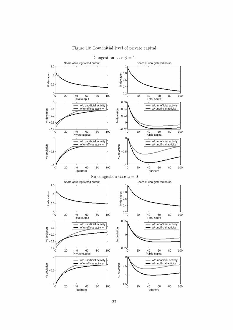
Figure 10: Low initial level of private capital
Congestion case φ = 1
0 20 40 60 80 1000
0.5
1
1.5
% d
evia
tion
Share of unregistered output
0 20 40 60 80 1000.2
0.4
0.6
0.8
1
% d
evia
tion
Share of unregistered hours
0 20 40 60 80 100−0.4
−0.3
−0.2
−0.1
0
% d
evia
tion
Total output
w/o unofficial activityw/ unofficial activity
0 20 40 60 80 100−0.02
0
0.02
0.04
0.06
% d
evia
tion
Total hours
w/o unofficial activityw/ unofficial activity
0 20 40 60 80 100−1
−0.5
0
quarters
% d
evia
tion
Private capital
w/o unofficial activityw/ unofficial activity
0 20 40 60 80 100−1
−0.5
0
quarters
% d
evia
tion
Public capital
w/o unofficial activityw/ unofficial activity
No congestion case φ = 0
0 20 40 60 80 1000
0.5
1
1.5
% d
evia
tion
Share of unregistered output
0 20 40 60 80 1000.2
0.4
0.6
0.8
1
% d
evia
tion
Share of unregistered hours
0 20 40 60 80 100−0.4
−0.3
−0.2
−0.1
0
% d
evia
tion
Total output
w/o unofficial activityw/ unofficial activity
0 20 40 60 80 100−0.05
0
0.05
% d
evia
tion
Total hours
w/o unofficial activityw/ unofficial activity
0 20 40 60 80 100−1
−0.5
0
quarters
% d
evia
tion
Private capital
w/o unofficial activityw/ unofficial activity
0 20 40 60 80 100−1.5
−1
−0.5
0
quarters
% d
evia
tion
Public capital
w/o unofficial activityw/ unofficial activity
27

low compared to the long-run costs. Figure 11 illustrates this intertemporaltrade-off.
Figure 11: Welfare losses along the transitional dynamics
Congestion case φ = 1 No congestion case φ = 0
0 20 40 60 80 100−0.18
−0.16
−0.14
−0.12
−0.1
−0.08
−0.06
−0.04
−0.02
quarters
% o
f ste
ady−
stat
e co
nsum
ptio
n
Low initial condition on private capital
w/o unofficial activityw/ unofficial activity
0 20 40 60 80 100−0.2
−0.15
−0.1
−0.05
0
quarters
% o
f ste
ady−
stat
e co
nsum
ptio
n
Low initial condition on private capital
w/o unofficial activityw/ unofficial activity
A low quantity of public physical capital
Economies in transition from communism may also experience a relatively lowlevels of productive services, because of low initial fiscal revenues. Johnson etal. [1998] argue along these lines that ‘most of the former Soviet Union is stuckin a bad equilibrium with low tax revenue, high unofficial economy as a per-centage of GDP, and low quality of publicly provided services’. The downwardspiral comes from the fact that the quality of public services is what providesthe incentive for firms to register and income tax are requested to finance pub-lic expenditures. Public expenditures are in this exercise endogenous, becausewe add a constant transfers-to-registered output to the balanced-budget re-quirement. We can however impose a low level of public services through theassumption that the initial stock of capital infrastructures is below its long-runlevel. Figure 12 displays the evolution of output and hours when the econ-omy starts with a stock of public infrastructures 1% lower than its steady–statelevel. Once again, the grey lines, where present, describe a benchmark economywithout underground production.
Public and private capital both serve as inputs to the production functionof registered firms. A low quantity of public services and infrastructure doesstimulate participation to the underground activity and yields reduction in totaloutput as did low levels of private capital. Mid-term dynamics however differin the two variants, due to distinct accumulation paths: the decrease in privatecapital is more than 5 times lower than were the reduction in public capital.Households do modify their investment plans as the marginal product revenue of
28

Figure 12: Low initial level of public capital
Congestion case φ = 1
0 20 40 60 80 1000.1
0.15
0.2
0.25
% d
evia
tion
Share of unregistered output
0 20 40 60 80 1000.1
0.12
0.14
0.16
0.18
% d
evia
tion
Share of unregistered hours
0 20 40 60 80 100−0.08
−0.06
−0.04
−0.02
% d
evia
tion
Total output
w/o unofficial activityw/ unofficial activity
0 20 40 60 80 100−0.04
−0.03
−0.02
−0.01
0
% d
evia
tion
Total hours
w/o unofficial activityw/ unofficial activity
0 20 40 60 80 100−0.2
−0.15
−0.1
−0.05
0
quarters
% d
evia
tion
Private capital
w/o unofficial activityw/ unofficial activity
0 20 40 60 80 100−1
−0.5
0
quarters
% d
evia
tion
Public capital
w/o unofficial activityw/ unofficial activity
No congestion case φ = 0
0 20 40 60 80 1000.1
0.15
0.2
0.25
% d
evia
tion
Share of unregistered output
0 20 40 60 80 1000.1
0.15
0.2
0.25
% d
evia
tion
Share of unregistered hours
0 20 40 60 80 100−0.1
−0.08
−0.06
−0.04
% d
evia
tion
Total output
w/o unofficial activityw/ unofficial activity
0 20 40 60 80 100−0.06
−0.04
−0.02
0
% d
evia
tion
Total hours
w/o unofficial activityw/ unofficial activity
0 20 40 60 80 100−0.2
−0.15
−0.1
−0.05
0
quarters
% d
evia
tion
Private capital
w/o unofficial activityw/ unofficial activity
0 20 40 60 80 100−1
−0.8
−0.6
−0.4
−0.2
quarters
% d
evia
tion
Public capital
w/o unofficial activityw/ unofficial activity
29

private capital increase, whereas public investment remained determined by thebalance budget requirement, because we considered constant tax rates. Hence,the negative effect of an initial lack of public capital are by far more moderate,and the transition from this initial condition is quicker.18
Congestion slightly modifies output shares though; this can be best illus-trated in the case of a high initial condition on public physical capital (justreverse the graphs). A high level of public capital Gt induces a raise in totaloutput, which partially offset the positive effect on the ratio of public capital tototal output Gt
Yt+Yt, which is the measure of productive public services. Because
the external effect is less positive when public capital is subject to congestion,the increase in the output of the registered activity is lower when φ = 1 thanwhen φ = 0. Therefore, the share of the underground economy in official outputwould be higher in the congestion case if there were ‘too much’ public capital.Here, we see that Yt
Ytis smaller when φ > 0 than when φ = 0.
Figure 13: Welfare losses along the transitional dynamics
Congestion case φ = 1 No congestion case φ = 0
0 20 40 60 80 100−0.035
−0.03
−0.025
−0.02
−0.015
−0.01
quarters
% o
f ste
ady−
stat
e co
nsum
tion
Low initial condition on public capital
w/o unofficial activityw/ unofficial activity
0 20 40 60 80 100−0.045
−0.04
−0.035
−0.03
−0.025
−0.02
−0.015
quarters
% o
f ste
ady−
stat
e co
nsum
tion
Low initial condition on public capital
w/o unofficial activityw/ unofficial activity
A low total factor productivity
Our third experiment is to assume that the physical capital stock has convergedbut that the total factor productivity (TFP) is below its long-run level. Severalfactors can explain the low level of productivity in transition economies. Thephysical capital stock may still be of a lower quality19 than in the balanced–growth path, even if the quantity of physical capital has converged and despitethe large investment effort that has been taken in both republics in the recentyears — for example, the capital stock in buildings, structures, machinery and
18Canova and Ravn [2000] emphasize the role of taxes in another example of transition, theGerman reunification. In their work, taxes only finance redistributive transfers and have toincrease when the demographic shock occurs.
19The average age of capital could proxy this effect in an empirical exercise.
30

equipment has increased by more than 15% from 1994 to 1997 in the CzechRepublic. Alternatively, the match between education of the labor force andphysical capital may be poor.
Figure 14 displays the evolution of output and hours when firms operatingin both activities start with an exogenous total factor productivity 1% lowerthan its steady–state level, but catching up the deterministic trend γt
x followinga first-order auto-regressive process.
As in the two previous exercises, total output starts from a low initial out-put. Note that the percent deviation from the long–run level of output exceedsmarkedly 1%, which is the discrepancy mechanically implied by a 1% deviationin total factor productivity, Γt. Therefore, smaller factor quantities or factormis-allocation must arise at this stage.
Labor supply is part of the explanation. Because of the transitory low re-ward for labor in the registered activity, households substitute labor intertem-porally and enjoy more leisure today. They also substitute intratemporallytowards the unregistered activity, as the upper-right panel show.
The low level of output has a large negative effect on both private andpublic capital accumulation. Ten years after the negative productivity shock,private and public capital respectively lie 2 and 4% below their long-run values.Needless to say, the relative size of the underground economy is then higherthan average. From that point, the economy experiences a slow recovery whichresembles the mid-term dynamics previously encountered. The existence of anunderground activity slows the transition process.
4.2 A transition scenario
In the previous three exercises, we have described analytically the adjustmentpaths associated with one deviation from the balanced growth path. This meansthat, of the private stock of physical capital, the public stock of capital and thetotal factor productivity, only one state variable were not equal to its balancedgrowth path value. We have however seen how these three state variableswere affecting each other: for example, a lack of private capital was inducinga serious decrease of public capital, away from its long-run value. We havealso emphasized how a typical transition economy, such as the Czech or theSlovak Republic, was currently experiencing low levels of private capital, publicservices and infrastructures and total factor productivity simultaneously.
Hence, we turn to a more descriptive type of exercise. We draw a transitionscenario which results can be interpreted as a weighted sum of the previousthree polar cases: what happens in this model economy when private capital isinitially x% lower than its long-run value, when public capital is y% lower and
31

Figure 14: Low initial level of factor productivity
Congestion case φ = 1
0 20 40 60 80 100−1
0
1
2
3
% d
evia
tion
Share of unregistered output
0 20 40 60 80 100−1
0
1
2
3
% d
evia
tion
Share of unregistered hours
0 20 40 60 80 100−1.5
−1
−0.5
0
% d
evia
tion
Total output
w/o unofficial activityw/ unofficial activity
0 20 40 60 80 100−0.8
−0.6
−0.4
−0.2
0
% d
evia
tion
Total hours
w/o unofficial activityw/ unofficial activity
0 20 40 60 80 100−2
−1.5
−1
−0.5
0
quarters
% d
evia
tion
Private capital
w/o unofficial activityw/ unofficial activity
0 20 40 60 80 100−6
−4
−2
0
quarters
% d
evia
tion
Public capital
w/o unofficial activityw/ unofficial activity
No congestion case φ = 0
0 20 40 60 80 100−2
0
2
4
% d
evia
tion
Share of unregistered output
0 20 40 60 80 100−1
0
1
2
3
% d
evia
tion
Share of unregistered hours
0 20 40 60 80 100−2
−1.5
−1
−0.5
% d
evia
tion
Total output
w/o unofficial activityw/ unofficial activity
0 20 40 60 80 100−1
−0.5
0
% d
evia
tion
Total hours
w/o unofficial activityw/ unofficial activity
0 20 40 60 80 100−3
−2
−1
0
quarters
% d
evia
tion
Private capital
w/o unofficial activityw/ unofficial activity
0 20 40 60 80 100−6
−4
−2
0
quarters
% d
evia
tion
Public capital
w/o unofficial activityw/ unofficial activity
32

Figure 15: Welfare losses along the transitional dynamics
Congestion case φ = 1 No congestion case φ = 0
0 20 40 60 80 100−0.55
−0.5
−0.45
−0.4
−0.35
−0.3
−0.25
−0.2
−0.15
quarters
% o
f ste
ady−
stat
e co
nsum
ptio
n
Low initial condition on factor productivity
w/o unofficial activityw/ unofficial activity
0 20 40 60 80 100−0.7
−0.6
−0.5
−0.4
−0.3
−0.2
quarters
% o
f ste
ady−
stat
e co
nsum
ptio
n
Low initial condition on factor productivity
w/o unofficial activityw/ unofficial activity
total factor productivity z% lower? Were we able to estimate precisely thesediscrepancies, this exercise would have some kind of prospective power. But weunfortunately are not and this experiment remains only illustrative. Anotherobvious limitation is the closed–economy assumption, as compared to the roleof foreign–direct investment in the transition process of Central and EasternEuropean countries.20
The relative deviations from the balanced–growth path we have consideredare the following: 10% on private capital, 2% on public capital and 5% on totalfactor productivity. Figure 16 displays the predicted transition paths as well astheir long–run counterpart.
The upper panels show that the relative size of the underground economyis larger than average, as was the case in any of the three polar experiment. Itis also rising in the first five years of transition. This was the pattern observedin the public capital and factor productivity experiments, but not from a lowinitial condition on private capital. We can therefore predict that the size of thehidden economy should mildly increase in the Czech and Slovak Republics overthe coming years unless unless the lack of private capital is more pronounced(relative to the lack of public capital and to the low TFP) than what we haveassumed. The model also predicts that this rise does not come from a long-runtrend and that the share of unregistered output will eventually decrease.
In terms of welfare, the first years of this transition scenario are very harmfulsince the expected present value of future utility flows is actually decreasing forthe first three years — this means that the representative household wouldbe willing to give up a larger amount of consumption forever rather than to
20Barry, Bradley, Kejak and Vavra [2000] present alternative transition scenarios for theCzech Republic.
33

Figure 16: A transition scenario
Congestion case φ = 1
20 40 60 80 1000.1
0.15
0.2
0.25
quarters
perc
enta
ge p
oint
s
Output share of the underground sector
20 40 60 80 1000.1
0.15
0.2
0.25
quarterspe
rcen
tage
poi
nts
Hours share of the underground sector
0 20 40 60 80 1001
1.5
2
2.5
3
quarters
Total output
path trend
20 40 60 80 1000.35
0.4
0.45
quarters
Total hours
No congestion case φ = 0
20 40 60 80 1000.1
0.15
0.2
0.25
quarters
perc
enta
ge p
oint
s
Output share of the underground sector
20 40 60 80 1000.1
0.15
0.2
0.25
quarters
perc
enta
ge p
oint
s
Hours share of the underground sector
0 20 40 60 80 1001.4
1.6
1.8
2
2.2
2.4
2.6
2.8
quarters
Total output
path trend
20 40 60 80 1000.35
0.4
0.45
quarters
Total hours
34
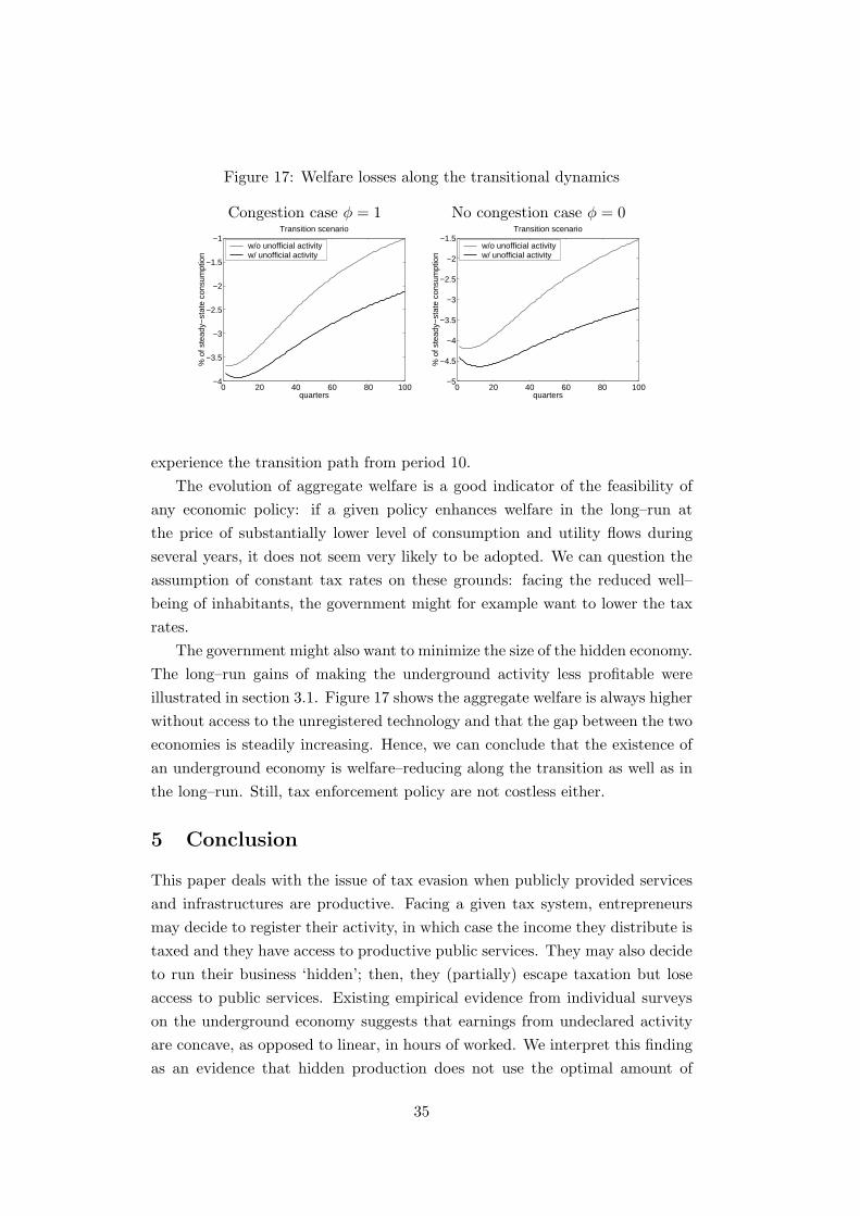
Figure 17: Welfare losses along the transitional dynamics
Congestion case φ = 1 No congestion case φ = 0
0 20 40 60 80 100−4
−3.5
−3
−2.5
−2
−1.5
−1
quarters
% o
f ste
ady−
stat
e co
nsum
ptio
n
Transition scenario
w/o unofficial activityw/ unofficial activity
0 20 40 60 80 100−5
−4.5
−4
−3.5
−3
−2.5
−2
−1.5
quarters
% o
f ste
ady−
stat
e co
nsum
ptio
n
Transition scenario
w/o unofficial activityw/ unofficial activity
experience the transition path from period 10.The evolution of aggregate welfare is a good indicator of the feasibility of
any economic policy: if a given policy enhances welfare in the long–run atthe price of substantially lower level of consumption and utility flows duringseveral years, it does not seem very likely to be adopted. We can question theassumption of constant tax rates on these grounds: facing the reduced well–being of inhabitants, the government might for example want to lower the taxrates.
The government might also want to minimize the size of the hidden economy.The long–run gains of making the underground activity less profitable wereillustrated in section 3.1. Figure 17 shows the aggregate welfare is always higherwithout access to the unregistered technology and that the gap between the twoeconomies is steadily increasing. Hence, we can conclude that the existence ofan underground economy is welfare–reducing along the transition as well as inthe long–run. Still, tax enforcement policy are not costless either.
5 Conclusion
This paper deals with the issue of tax evasion when publicly provided servicesand infrastructures are productive. Facing a given tax system, entrepreneursmay decide to register their activity, in which case the income they distribute istaxed and they have access to productive public services. They may also decideto run their business ‘hidden’; then, they (partially) escape taxation but loseaccess to public services. Existing empirical evidence from individual surveyson the underground economy suggests that earnings from undeclared activityare concave, as opposed to linear, in hours of worked. We interpret this findingas an evidence that hidden production does not use the optimal amount of
35

physical capital, or that concealment costs rise with the size of physical capitalused in underground production.
Participation decisions of labor suppliers depend on the earnings differentialbetween the two types of activities. Contrary to the partial equilibrium litera-ture, these earnings — the official and unofficial wage rates — vary to clear thelabor market, for example when the tax system is modified. The relative sizeof the underground economy, at the market clearing equilibrium, reflects theinstitutional characteristics as well as available technologies and preferences.According to a calibration relying on Czech National Accounts, this long–runequilibrium size would be between 15 to 20%, which is in the upper band ofcurrent macro–estimates for this country.
Two kinds of experiments are undertaken in this framework. First, thesteady–state effects of different economic policy regarding the tax system areevaluated.
• We first consider an increase in the efficiency of the fraud detection, whichhalves the gain to participate to the underground sector and therefore hasa social cost. This policy induces a permanent increase in consumptionof more than 5%, but does not take into account any additional fundingfor the tax agency.
• Our second run of policy experiments concerns variations in the tax rates.Two type of linear taxes are introduced: an income tax and a consumptiontax, or VAT. In both cases, endogenous fiscal evasion behaviors shift theLaffer curve, which is the (non–monotonic) relationship between tax ratesand fiscal revenues. For example, the largest fiscal revenues are attainedfor an income tax rate around 40% when agents cannot evade taxes; butit is as low as 25% once entrepreneurs have access to the unregisteredactivity. The conventional wisdom is that an underground productionlimits the tax–induced distortions. When a trade–off between fiscal dis-tortions and financing of productive public services is allowed, an optimallevel of underground production arises. Because of this effects, optimalpublic investment rules are modified: the income tax rate that maximizeswelfare is below the elasticity of (registered) output with respect to publiccapital.
• In a related exercise, we modify the share of fiscal revenues carried bythe income tax. In this representative agent setup, output and aggregatewelfare are maximized when the consumption tax bears all the tax burden,whether agents have access to underground production or not. Efficiencyand equity apparently yield opposite policy recommendations.
36

The second type of experiment we have run is more specific to the transi-tion process. We study the dynamics of our model economy starting from initialconditions below the balanced–growth path. In polar cases when either privatecapital or public capital or factor productivity deviates from its long–run level,we see that the relative size of the underground economy is temporarily higherthan average. Compared to a benchmark economy without underground out-put, the speed of adjustment is also significantly slower. In a second stage, webuild up a transition scenario where the economy simultaneously lacks of privatecapital and public services, and with low factor productivity. This exercise pre-dicts that the relative size of the underground economy should increase duringthe first years of transition and return eventually to the long–run level, unlessthe stock of private physical capital is surprisingly low as compared to publiccapital. It also predicts that aggregate welfare is higher when no undergroundproduction takes place at any horizon of the transition process.
References
Allingham, M.G. and A. Sandmo, Income tax evasion: a theoretical analysis,Journal of Public Economics, 1972, 1, 323–338.
Asea, P.K., The informal sector: baby or bath water?, Carnegie-RochesterConference Series, 1996, 45, 163–171.
Barro, R.J., Government spending in a simple model of endogenous growth,Journal of Political Economy, 1990, 98 (5), S103–S125.
Barry, F., J. Bradley, M. Kejak, and D. Vavra, The Czech economic transition:exploring options using a macrosectoral model, Working Paper, UniversityCollege Dublin January 2000.
Canova, F. and M.O. Ravn, The macroeconomic effects of German unification:real adjustments and the welfare state, Review of Economic Dynamics,2000, 3 (3), 423–460.
Caragata, P.J. and D.E.A. Giles, Simulating the relationship between the hid-den economy and the tax level and tax mix in New Zealand, in G.W. Scullyand P.J. Caragata, editors, Taxation and the limits of government, Boston:Kluwer, 2000.
Christiano, L.J., Understanding Japan’s saving rate: the reconstruction hy-pothesis, Federal Reserve Bank of Minneapolis Quarterly review, 1989, 13(2), 10–25.
37

Cooley, T.F. and E. C. Prescott, Economic growth and business cycles, inT.F. Cooley, editor, Frontiers of business cycle research, Princeton, NJ:Princeton University Press, 1995, chapter 1, pp. 1–39.
Easterly, W., How much do distortions affect growth?, Journal of MonetaryEconomics, 1993, 32, 187–212.
Fortin, B., G. Lacroix, and C. Montmarquette, Are underground workersmore likely to be underground consumers?, Economic Journal, forthcom-ing 2000.
, N. Marceau, and L. Savard, Taxation, wage controls and the informalsector, Journal of Public Economics, 1997, 6, 293–312.
Hurlin, C., La contribution productive des infrastructures: analyses positiveset normatives. PhD dissertation, Universite Paris I 2000.
Johnson, S., D. Kaufmann, and P. Zoido-Lobaton, Regulatory discretion andthe unofficial economy, American Economic Review, May 1998, 88 (2),387–392.
, , J. McMillan, and C. Woodruff, Why do firms hide? Bribes andunofficial activity after communism, Journal of Public Economics, 2000,76, 495–520.
Jung, Y.H., A. Snow, and G.A. Trandel, Tax evasion and the size of theunderground economy, Journal of Public Economics, 1994, 54, 391–402.
Kesselman, J. R., Income tax evasion: an intersectorial analysis, Journal ofPublic economics, 1989, 38, 137–182.
King, R.G and S.T. Rebelo, Transitional dynamics and economic growth in theneoclassical model, American Economic Review, 1993, 83 (4), 908–931.
Kleven, H.J., W.F. Richter, and P.B. Sørensen, Optimal taxation with house-hold production, Oxford Economic Papers, 2000, 52, 584–594.
Lemieux, T., B. Fortin, and P. Frechette, The effect of taxes on labor supplyin the underground economy, American Economic Review, 1994, 84 (1),231–254.
Loayza, N.V., The economics of the informal sector: a simple model and someempirical evidence from Latin America, Carnegie-Rochester ConferenceSeries, 1996, 45, 129–162.
38

OECD, Czech Republic, OECD Economic Studies, February 2000, 2000 (4).
Piggott, J. and J. Whalley, VAT base broadening, self supply, and the informalsector, Working Paper 6349, NBER January 1998.
Rogerson, R., Indivisible labor, lotteries and equilibrium, Journal of MonetaryEconomics, 1988, 21 (1), 3–17.
Sandmo, A., Income tax-evasion, labour supply, and the equity-efficiency trade-off, Journal of Public Economics, 1981, 16, 265–288.
, Tax distortions and household production, Oxford Economic Papers,1990, 42, 78–90.
Schneider, F. and D.H. Enste, Shadow economies: size, causes and conse-quences, Journal of Economic Literature, 2000, 38, 77–114.
Slemrod, J., Optimal taxation and optimal tax systems, Journal of EconomicPerspectives, winter 1990, 4 (1), 157–178.
and S. Yitzhaki, The optimal size of a tax collection agency, ScandinavianJournal of economics, September 1987, 89, 183–192.
Thomas, J., Quantifying the black economy: ‘Measurement without theory’yet again?, Economic Journal, 1999, 109 (456), F381–F389.
Trandel, G.A. and A. Snow, Progressive income taxation and the undergroundeconomy, Economic Letters, 1999, 62, 217–222.
Yitzhaki, S., A note on income tax evasion: a theoretical analysis, Journal ofPublic Economics, 1974, 3, 201–202.
39