University College London

Department of Mathematics

The fluid dynamics

of chocolate fountains

Adam K. Townsend

adamtownsend.com

Supervisor: Dr Helen J. Wilson

M.Sci. Project in Mathematics

March 2012

2

Contents

1 Introduction 5

1.1 Modelling chocolate . . . . . . . . . . . . . . . . . . . . . . . . . . . 5

1.2 Typical values . . . . . . . . . . . . . . . . . . . . . . . . . . . . . . 9

2 The pipe 11

2.1 Newtonian, isothermal model . . . . . . . . . . . . . . . . . . . . . 11

2.2 Power-law fluid . . . . . . . . . . . . . . . . . . . . . . . . . . . . . 14

2.3 Casson’s model . . . . . . . . . . . . . . . . . . . . . . . . . . . . . 17

2.4 Generalised Newtonian fluid model . . . . . . . . . . . . . . . . . . 19

3 The dome 21

3.1 Isothermal Newtonian and power-law models . . . . . . . . . . . . . 21

3.2 Non-isothermal Newtonian model . . . . . . . . . . . . . . . . . . . 33

4 The falling sheet 41

4.1 Inviscid model . . . . . . . . . . . . . . . . . . . . . . . . . . . . . . 41

4.2 Viscous model . . . . . . . . . . . . . . . . . . . . . . . . . . . . . . 50

4.3 The teapot effect . . . . . . . . . . . . . . . . . . . . . . . . . . . . 51

4.4 Concluding remarks on the falling sheet . . . . . . . . . . . . . . . . 55

Bibliography 57

3

4

Chapter 1

Introduction

Chocolate fountains are a popular feature at special events. Melted chocolate ispumped over a series of domes and falls freely between them. In this project wemodel different fluid types over one such dome, and investigate how the fluid behavesin the different regions of the fountain: as it comes up the pipe (chapter 2), as itfalls down the dome (chapter 3), how it leaves the dome, and how it falls freely(chapter 4). When fluid leaves the dome, it is observed that the fluid falls inwardsrather than straight down and we offer an explanation and model for this.

Standard table chocolate fountains, such as in Figure 1.1, have two tiers and asmall pool at the top for chocolate to gather before it travels down the edge andtravels down the first dome. Chocolate is carried from the pool at the bottom ofthe fountain to the top by use of an Archimedes screw, but the existence of thepool at the top serves to remove all rotation in the fluid by the time it falls off.For this reason, and because axisymmetric pipe flows with pressure gradients are anice introduction to the fluid models we will be discussing, we model the pipe asa vertical axisymmetric pipe with a constant pressure gradient. We then continueour mathematical considerations on the dome as the fluid approaches from the top.This model is shown in Figure 1.2.

Experimentally it was observed that in our fountain, the temperature of the chocol-ate remains constant (at 40 ◦C to within one degree) throughout its journey in thefountain so long as the fountain has been running for long enough (about thirtyminutes). Wollny (2005) states that to within one degree, viscosity of chocolateshould fluctuate between 5% and 10%. The much greater influence on viscosity isshear stress, which we consider in following chapters.

1.1 Modelling chocolate

When we consider different fluid models, what we are considering is the relationship(called the constitutive relation) between the stress and velocity gradient tensors

5

MATHM901 The fluid dynamics of chocolate fountains

Figure 1.1: The chocolate fountain we are modelling in action.

Figure 1.2: We model the chocolate fountain as a hemisphere atop a vertical cylindricalpipe, capturing the essence of the problem.

6

Chapter 1. Introduction

within the fluid. Formally, for a stress tensor σ and velocity vector u,

σ = F (∇u,∇u|t<t0 , . . .) ,

where F is a functional which can take a multitude of arguments, possibly including:velocity gradient, temperature, electric fields, time, the scalar shear rate γ (definedbelow), and historical (t < t0) values of all these quantities.

The shear rate tensor, γ, is defined as

γ = ∇u+∇uT

and its scalar counterpart, γ, is defined as

γ =

(1

2∇u : ∇u

)1/2

=

(γabγab2

)1/2

, (1.1)

where γij is the ijth component of γ.

In a generalised Newtonian fluid, the functional F is a function µ of γ alone, andrepresents the viscosity,

σ = µ(γ)γ,

and component-wise,σij = µ(γ)γij,

where σij is the ijth component of σ. It is from this family of models that weshall choose to model chocolate in our chocolate fountain, since the temperaturethroughout the chocolate’s path in the fountain does not change enough to warrantcomplicating the model.

In a simple shear flow in a channel of height y and where the top of the channelis moving with speed u, as in Figure 1.3, the shear rate tensor is simply the scalarvalue

γ = γ =∂u

∂y

and hence for a generalised Newtonian fluid,

σ = µ(γ)γ = f(γ),

for some ‘combined’ function f . It is customary to introduce fluid models in thissimple shear flow first, so this is how we shall proceed.

The simplest fluid model we shall be using is the Newtonian model, where thereis proportionality between stress and strain rate,

σ = µγ,

and our viscosity µ is a constant. We shall be using a representative viscosity ofchocolate at the sort of shear rates we are expecting (about 10 s−1) of 14Pa s. Theviscosity of honey is 10Pa s so this is a sensible value.

7

MATHM901 The fluid dynamics of chocolate fountains

Figure 1.3: Shear flow in a 2D channel of height y with a fixed base and a stressapplied to the top, causing the top to move at a speed u.

In Casson (1959), N. Casson provides a model, originally designed for printing ink,which gives a constitutive equation of

√σ =

{ √µcγ +

√σy if σ ≥ σy√

σy if σ ≤ σy(1.2)

where µc is the Casson plastic viscosity, and σy is the yield stress, given in pipe flowby

σy =rcσwa

(1.3)

where rc is the critical radial value (the value for which we expect plug flow), σw isthe stress upon the pipe wall, and a is the radius of the pipe.

Typical values for chocolate, from industrial experiments (Mongia and Ziegler, 2000),are given in Table 2.1, where we explore this model more. This model, Casson’s

model, was recommended by the International Confectionery Association to modelchocolate from 1973 until 2000, when Aeschlimann and Beckett (2000) found thatat low shear rates, Casson’s model does not fit the experimental rheology datawell. As such it was difficult to find repeatability, and so interpolation data wasrecommended instead. (Sahin and Sumnu, 2006; Afoakwa et al., 2009).

Such interpolation data typically takes the form of a power-law model, where

σ = kγn.

In component form, which we will use both in the pipe and on the dome in thefollowing chapters, this is equivalent to

σij = kγn−1γij (1.4)

where γ is that scalar shear rate defined in equation (1.1). Typical values forchocolate at 40 ◦C are, from industrial experiment (Radosasvljevic et al., 2000),k = 65 and n = 0.3409. Fluids with n < 1, as our chocolate is, are called shear-thinning, and include ceiling paint and tomato ketchup∗ among them. Fluids withn > 1 are called shear-thickening, of which a paste of cornflour and water is the bestknown. Of course, when n = 1, this model is equivalent to the Newtonian model.These relations are shown in Figure 1.4.

∗Ketchup is actually a more special type of shear-thinning fluid, a Bingham fluid.

8

Chapter 1. Introduction

Figure 1.4: Graph of stress against rate of strain for a typical shear-thickening(dark red), Newtonian (orange), shear-thinning (blue) and Bingham fluid(green).

1.2 Typical values

At points in this project, we use experimental data to argue relative size of terms, orto compare expected result with what we observe in the chocolate fountain. Table1.1 lists the typical values found from experiment, and relevant sources.

∗Source: Radosasvljevic et al. (2000)§Source: Keijbets et al. (2009). Experiments done with dark chocolate (50% cocoa), but this

number is representative.‡Source: Wichchukit et al. (2005). Experiments done with milk chocolate at 42 ◦C.¶Source: Daubert et al. (1997). Experiments done with milk chocolate over a temperature

range 25–60 ◦C.

9

MATHM901 The fluid dynamics of chocolate fountains

Pipe radius a 0.02 mDome radius R 0.07 m

Density of chocolate‡ ρ 1270 kgm−3

Surface tension of chocolate§ γs 0.0226 Nm−1

Thermal diffusivity¶ c 6.32× 10−8 m2 s−1

Characteristic dome film thickness H 0.001 mCharacteristic dome velocity U 0.1 m s−1

Typical dome leaving velocity u0 0.1 m s−1

Characteristic sheet film thickness H 0.0015 mGravitational acceleration g 10 m s−2

Drop height ℓ 0.07 mNewtonian apparent viscosity µ 14 Pa s

Power-law flow consistency index∗ k 64.728 Pa sn

Power-law flow behaviour index∗ n 0.3409

Table 1.1: Table of values found experimentally

10

Chapter 2

The pipe

In a chocolate fountain, chocolate is heated at the bottom and is then transportedto the top using an Archimedes spiral (and it is the rotating of the spiral whichcreates the noise associated with running it). Such spirals are difficult to modeland since the rotation of the fluid makes observably minimal difference at the topof the fountain, we model the spiral as a vertical pipe with a constant pressuregradient. This choice of model also allows us to introduce relevant non-Newtonianfluid models within a geometry that is familiar and well-researched.

The radius of the pipe is a, and we will use cylindrical coordinates (r, θ, z) althoughthe axisymmetric nature of the problem will lead us to expect no motion in the θdirection.

2.1 Newtonian, isothermal model

In our first model we model the chocolate as a viscous, incompressible Newtonianfluid, with constitutive equation

σ = µγ

where µ is constant.

The Navier–Stokes equation for a viscous, incompressible Newtonian fluid is

ρDu

Dt= −∇p+ µ∇2u+ F (2.1)

where u is the velocity of the fluid, DDt

= ∂∂t+ u · ∇ is the material derivative, ρ is

the density of the fluid (assumed constant), µ is the viscosity of the fluid and F areexternal body forces (per unit volume).

Incompressibility gives us the continuity equation:

∇ · u = 0.

11

MATHM901 The fluid dynamics of chocolate fountains

In axisymmetric cylindrical polar coordinates, where the only external body forceacting is gravity (downwards), these two equations are equivalent to the followingsystem:

ρ

(∂ur∂t

+ ur∂ur∂r

+ uz∂ur∂z

)= −∂p

∂r+ µ

[1

r

∂

∂r

(r∂ur∂r

)+∂2ur∂z2

− urr2

](2.2)

ρ

(∂uz∂t

+ ur∂uz∂r

+ uz∂uz∂z

)= −∂p

∂z+ µ

[1

r

∂

∂r

(r∂uz∂r

)+∂2uz∂z2

]− ρg (2.3)

1

r

∂

∂r(rur) +

∂uz∂z

= 0. (2.4)

We expect steady flow, so we can say that

∂ur∂t

=∂uz∂t

= 0.

Furthermore by symmetry we only expect flow in the z-direction, so we set

ur = 0 and uz = u(r).

The three equations above then reduce to:

0 = −∂p∂r

(2.5)

0 = −∂p∂z

+ µ

[1

r

∂

∂r

(r∂u

∂r

)]− ρg (2.6)

0 = 0. (2.7)

Equation (2.5) tells us that p = p(z, t) and equation (2.6) is the only thing left tosolve.

We are assuming a constant pressure gradient

∂p

∂z= G = const.

with the boundary conditions

u(a) = 0 no-slip condition (2.8)

∂u

∂r(0) = 0 by symmetry (2.9)

If we letH = −(G+ ρg),

the total pressure gradient including hydrostatic pressure, then equation (2.6) canbe written

−H =µ

r

∂

∂r

(r∂u

∂r

)

12

Chapter 2. The pipe

-0.02 -0.01 0.01 0.02

-0.10

-0.08

-0.06

-0.04

-0.02

Figure 2.1: Velocity profile of a Newtonian fluid, given by (2.10). The pressure gradi-ent G is set to zero, hence we get downwards flow in the pipe. Constantsare from Table 1.1

Rearranging and integrating once with respect to r,

−r2H2µ

+ C = r∂u

∂r.

Rearranging and integrating with respect to r again,

−r2H4µ

+ C ln r +D = u.

Boundary condition (2.8) tells us

D =a2H

4µ− C ln a

and boundary condition (2.9) gives C = 0 and so

u =a2H

4µ− r2H

4µ

and substituting in H gives

u = (r2 − a2)G+ ρg

4µ, (2.10)

our velocity profile for a Newtonian fluid in a pipe with constant pressure head(Poiseuille flow). Note that we shouldn’t be worried that r2−a2 is mostly negative:in the absence of a pressure gradient G, we would, of course, expect fluid to falldown the tube, in the −z-direction. Figure 2.1 shows this velocity profile, in theabsence of a pressure gradient, which is a parabola.

13

MATHM901 The fluid dynamics of chocolate fountains

2.2 Power-law fluid

We consider a power-law fluid travelling up a vertical pipe. The Navier–Stokesequation for a general fluid is

ρDu

Dt= −∇p+∇ · σ + F (2.11)

(which reduces to (2.1) for a Newtonian fluid) where σ is the stress tensor (notethat some authors include the pressure within their definition of the stress tensor).Expanded into cylindrical polar coordinates for an axisymmetric flow, where down-wards gravity is the only external force, this is equivalent to

ρ

(∂ur∂t

+ ur∂ur∂r

+ uz∂ur∂z

)= −∂p

∂r−[1

r

∂

∂r(rσrr)−

σθθr

+∂σrz∂z

](2.12)

ρ

(∂uz∂t

+ ur∂uz∂r

+ uz∂uz∂z

)= −∂p

∂z−

[1

r

∂

∂r(rσzr) +

∂σzz∂z

]− ρg (2.13)

1

r

∂

∂r(rur) +

∂

∂z(uz) = 0. (2.14)

Steady flow demands∂ur∂t

=∂uz∂t

= 0

and by symmetry we expect flow only in the z-direction, so we set

ur = 0 and uz = uz(r).

We now seek to find which components of stress become zero under these velocityassumptions. For a generalised Newtonian fluid, such as the power-law model we’reusing here, if a given component of γ is zero, then the respective component of σis too. For the power-law model, this is explicit in equation (1.4). In cylindricalcoordinates, the components of rate of strain γ for an incompressible fluid are givenby

γrr = 2∂ur∂r

γθθ = 2

(1

r

∂uθ∂θ

+urr

)

γzz = 2∂uz∂z

γrθ = γθr = r∂

∂r

(uθr

)+

1

r

∂ur∂θ

γrz = γzr =∂uz∂r

+∂ur∂z

(2.15)

γθz = γzθ =∂uθ∂z

+1

r

∂uz∂θ

.

Under the assumptions uθ = ur = 0 and uz = uz(r), the only non-zero componentof γ is γrz and so the only non-zero component of σ is σrz = σzr.

14

Chapter 2. The pipe

With this in mind then, equations (2.12)–(2.14) reduce to

0 = −∂p∂r

(2.16)

0 = −∂p∂z

+1

r

∂

∂r(rσzr)− ρg (2.17)

0 = 0. (2.18)

We notate the steady pressure gradient thus,

∂p

∂z= G = const.

and for convenience we add the gravity term to form the pressure head, H,

H = −(G+ ρg).

We are then left to solve∂

∂r(rσzr) = Hr

which after integration with respect to r and rearranging gives

σzr =Hr

2. (2.19)

Note that the constant of integration is set to zero by the boundary condition thatσzr(0) = 0 by symmetry. Introducing the wall stress,

σw =Ha

2,

equation (2.19) is equivalent to

σzr = σwr

a. (2.20)

Equation (1.4) tells usσzr = kγn−1γzr,

and equation (2.15) tells us

γ = γzr =duzdr

, (2.21)

where γ is our scalar shear rate, given by (1.1), and equal to γzr since it is the onlynon-zero component of strain rate.

Substituting this into equation (2.20) gives

k

(duzdr

)n

= σwr

a,

which we can rearrange to find an expression for duz/dr,

duzdr

=(σwka

)1/n

(r)1/n

15

MATHM901 The fluid dynamics of chocolate fountains

-0.02 -0.01 0.01 0.02

-0.04

-0.03

-0.02

-0.01

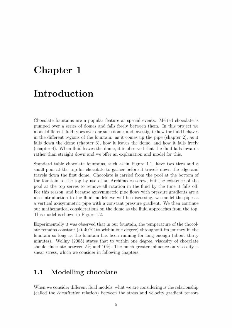
Figure 2.2: Velocity profile of a (shear-thinning) power-law fluid, given by (2.22).Constants are G = 0 (no pressure gradient, hence downward flow) andthe rest from Table 1.1

and then integrating with respect to r and noting the boundary condition uz(a) = 0,gives

uz =(σwka

)1/n r1+1/n − a1+1/n

1 + 1/n. (2.22)

In a Newtonian liquid, k = µ and n = 1 in equation (1.4) and substituting thesevalues into (2.22) gives us

uz =σwµa

r2 − a2

2

=H

2µ

r2 − a2

2

= (r2 − a2)G+ ρg

4µ

which is equivalent to equation (2.10).

Note that from our experimental data, the flow is slower with the power-law model:Figure 2.2 has been plotted with coefficients from the experimentally obtained datain Table 1.1, with the pressure gradient G once again set to zero (hence we getdownwards flow again). Maximum speed in the Newtonian model is 0.098ms−1 andthe maximum speed in the power-law model is 0.047ms−1. The model used herehas n = 1

3< 1: i.e. chocolate is modelled as a shear-thinning fluid. The shape of

the profile we see is somewhat similar to the parabola in the Newtonian case, but isconsiderably flatter at the centre: we see slower plug flow in the centre of the pipe,of width roughly a third of the diameter. Unlike in the Casson case which we shallsee next, however, the flatness in the centre is not totally flat, ∂uz/∂r 6= 0: there isstill some curvature.

16

Chapter 2. The pipe

2.3 Casson’s model

In chapter 1, we introduced Casson’s model, which gives a constitutive equation of

√σ =

{ √µCγ +

√σy if σ ≥ σy√

σy if σ ≤ σy

where µC is the Casson plastic viscosity, and σy is the yield stress, given by

σy =rcσwa

.

Recall equation (2.20):

σzr = σwr

a.

This time we square root this and substitute it into Casson’s model, equation (1.2),

√σwr

a=

√µCγ +

√σy, (2.23)

for σzr > σy. Solving for γzr gives

γzr =

(√σw

ra−√

σy)2

µC

,

or, substituting in equation (2.21),

duzdr

=

(√σw

ra−√

σy)2

µC

. (2.24)

We can integrate this with respect to r to find

uz = −r(8a

√σyrσw

a− 6aσy − 3rσw

)

6aµC

+ c.

Substituting in equation (1.3) for σy,

= −8r3/2r1/2c σw − 6rrcσw − 3r2σw

6aµC

+ c

= − σw2aµC

(8

3r3/2r1/2c − 2rrc − r2

)+ c,

and using the no-slip boundary condition u(a) = 0 we find

uz(r) =

{σw

2aµC

(83

(a3/2 − r3/2

)r1/2c − 2(a− r)rc − (a2 − r2)

)if rc ≤ r ≤ a

u(rc) if 0 ≤ rc < rc.

(2.25)

17

MATHM901 The fluid dynamics of chocolate fountains

Percentage of coarse chocolate powder σy (Pa) µC (Pa s)0 8.01 5.6025 6.64 3.7050 4.63 3.1775 2.79 3.60100 1.92 4.78

Table 2.1: Table of values found for σy and µC by Mongia and Ziegler (2000). Thedifferent chocolate samples were formed with a combination of coarse andfine chocolate powders, the percentages of which are given here.

-0.02 -0.01 0.01 0.02

-0.15

-0.10

-0.05

Figure 2.3: Velocity profile of a Casson fluid, given by (2.25). Constants are G = 0(no upward pressure gradient, hence downwards flow), µC = 4.63 (fromTable 2.1), rc = 6.71× 10−4 and the rest from Table 1.1.

-0.02 -0.01 0.01 0.02

-0.04

-0.03

-0.02

-0.01

Figure 2.4: Velocity profile of a Casson fluid, with the same values as Figure 2.3, butwith rc = 0.005 to emphasise the properties of this fluid model.

18

Chapter 2. The pipe

Mongia and Ziegler (2000) give values for σy and µC, reproduced in Table 2.1.Using this table, we can find an estimate for rc. If we use the value of σy for the50% sample, G = 0 and the values from Table 1.1 then

rc =σya

σw=

4.63× 0.02

1380× 10× 0.02/2= 6.71× 10−4

which is 3.4% of the radius of the pipe, so this is very small. This velocity profile hasbeen illustrated in Figure 2.3, and again in Figure 2.4 but with an artificially largercritical radius of rc = 0.005 to emphasise this property of Casson’s fluid model.With small rc, the profile looks very similar to the parabola seen in the Newtoniancase, with a slight flatness at the centre. With larger rc, it resembles much closerthe power-law profile, with the plug flow in the centre. This time, however, theflatness seen in both large and small rc is truly flat, ∂uz/∂r = 0 in this area.

2.4 Generalised Newtonian fluid model

The procedures for finding velocity profiles in the preceding sections can be gener-alised easily (Wilkinson, 1960).

If we have a constitutive relation

γ = f(σ), (2.26)

for some function f , then for pipe flow this is equivalent to

duzdr

= f(σzr). (2.27)

We can write the shear stress σzr in terms of the wall shear stress, σw, as

σzr = σwr

a.

Substituting this into (2.27) gives

duzdr

= f(σwr

a

),

and integrating with respect to r with the no-slip boundary condition u(a) = 0gives us our general velocity profile,

uz(r) =

∫ a

r

f(σwr

a

)dr. (2.28)

Of course the difficulty with this calculation is where the challenges lie, particularlysince the constitutive equation represented in equation (2.26) is conventionally writ-ten in the inverse, i.e.

σ = F (γ),

where F = f−1.

19

20

Chapter 3

The dome

3.1 Isothermal Newtonian and power-law models

In this section we model movement of chocolate over the dome, being released at aconstant rate from the very top of the dome. The resultant flow is described usinglubrication theory. We model the dome as the top half of a sphere, but show that theanalysis (and result) would work for any smooth shape, since the global curvatureof the dome does not affect the motion of the fluid (mirroring other thin-film flows).

We set up spherical coordinates (r, θ, φ) where θ is the inclination angle, 0 ≤ θ < π,and φ is the azimuthal angle, 0 ≤ φ < 2π. We label the radius of the sphere R andthe film thickness h. We expect axisymmetric flow so h = h(θ). This is summarisedin Figure 3.1.

We use and compare two fluid models: the Newtonian model and the power-lawmodel. We do not explore Casson’s model in this geometry since the algebra wouldbe considerably unwieldy, and we expect little difference between the Casson andpower-law models. The differences in pipe flow between the Casson and power-lawmodels, as seen in Figures 2.2 and 2.4, are very small anyway, and the differencebetween Newtonian and power-law flows (Figure 3.5) on the dome are in themselvesslight, so we expect very little noticable difference between the Casson and power-law models on the dome.

For a general fluid, the Navier–Stokes equation can be written

ρDu

Dt= −∇p+∇ · σ + F (2.11)

where ρ is our (constant) density, u = (ur, uθ, uφ) is our velocity vector, p is pressure,σ is our stress tensor, F = (Fr, Fθ, Fφ) are any external body forces (per unitvolume), and D/Dt is the material derivative.

We expect a steady, axisymmetric flow, so we set uφ = 0 and ∂/∂φ = 0. The

21

MATHM901 The fluid dynamics of chocolate fountains

Figure 3.1: Coordinate setup for the dome problem

Navier–Stokes equations can then be written out in component form as

ρ

[ur∂ur∂r

+uθr

∂ur∂θ

− u2θr

]

= −∂p∂r

−[1

r2∂

∂r

(r2σrr

)+

1

r sin θ

∂

∂θ(σrθ sin θ)−

σθθ + σφφr

]+ Fr (3.1)

ρ

[ur∂uθ∂r

+uθr

∂uθ∂θ

]

= −1

r

∂p

∂θ−

[1

r2∂

∂r

(r2σrθ

)+

1

r sin θ

∂

∂θ(σθθ sin θ) +

σrθr

− σφφ cot θ

r

]+ Fθ

(3.2)

0 = − 1

r sin θ

∂p

∂φ−[1

r2∂

∂r

(r2σrφ

)+

1

r

∂σθφ∂θ

+σrφr

+2σθφ cot θ

r

]+ Fφ (3.3)

and our continuity equation is

0 =1

r

∂

∂r

(r2ur

)+

1

sin θ

∂

∂θ(uθ sin θ) . (3.4)

We seek the form of the σ components, and since in both models that we are using,the stress is a direct function of the shear rate γ, we write out the shear componentsfor a general incompressible fluid, where we expect axisymmetric flow:

γrr = 2

[∂ur∂r

]

γθθ = 2

[1

r

∂uθ∂θ

+urr

]

γφφ = 2

[urr

+uθ cot θ

r

]

γrθ = γθr =

[r∂

∂r

(uθr

)+

1

r

∂ur∂θ

](3.5)

22

Chapter 3. The dome

γrφ = γφr = 0

γθφ = γφθ = 0

Since our fluid models in component form are

σij = µγij, σij = kγn−1γij

where γ =√γabγab/2 (using Einstein summation convention), zero shear rate leads

to zero stress component-wise. Hence the φ-momentum equation (3.3) reduces to

0 = − 1

r sin θ

∂p

∂φ+ Fφ. (3.6)

We now introduce gravity as our only external force, hence

(Fr, Fθ, Fφ) = (−ρg cos θ, ρg sin θ, 0).

This reduces our φ-momentum equation (3.6) to merely saying p = p(r, θ) (whichwe could have expected) and the r- and θ-momentum equations (3.1)–(3.2) become

ρ

[ur∂ur∂r

+uθr

∂ur∂θ

− u2θr

]

= −∂p∂r

−[1

r2∂

∂r

(r2σrr

)+

1

r sin θ

∂

∂θ(σrθ sin θ)−

σθθ + σφφr

]− ρg cos θ (3.7)

ρ

[ur∂uθ∂r

+uθr

∂uθ∂θ

]

= −1

r

∂p

∂θ−[1

r2∂

∂r

(r2σrθ

)+

1

r sin θ

∂

∂θ(σθθ sin θ) +

σrθr

− σφφ cot θ

r

]+ ρg cos θ.

(3.8)

Since this system is too complicated to solve analytically, we have to introduce ascaling which will allow us to neglect comparatively small terms. We rescale ourvariables in the following way

uθ =uθU, ur =

urV, h =

h

H, r =

r −R

H, (3.9)

where hats denote scaled variables. U and V are characteristic speeds in the θ- andr-direction respectively, H is a characteristic film thickness, and R is our already-established sphere radius. Note that our scaling for r is unusual, but it emphasisesthe physical nature of the problem: the fluid occupies the space R ≤ r ≤ R + h,and our scaling converts this into 0 ≤ r ≤ h/H, where h/H ∼ 1.

What this means for our scaling is that

uθ ∼ U, ur ∼ V, h ∼ H, r ∼ R, ∂/∂r ∼ 1/H. (3.10)

The continuity equation (3.4) tells us how these characteristic values interact witheach other. The equation is

0 =1

r

∂

∂r

(r2ur

)+

1

sin θ

∂

∂θ(uθ sin θ) .

23

MATHM901 The fluid dynamics of chocolate fountains

and soRV

H∼ U, (3.11)

where we have substituted our scalings for our variables. Strictly, this comes fromsubstituting our scaled variables (3.9) into the continuity equation, which wouldread

0 =1

Hr +R

1

H

∂

∂r

((R +Hr)2V ur

)+

1

sin θ

∂

∂θ(Uuθ sin θ) ,

and reading off the order of the terms. We will use the less strict approach inour forthcoming arguments, but strict treatment as shown here will give the sameresults. The important part of the equivalence (3.11) is that

V ∼ UH

R

which is very small compared to U , since H/R is small. Of course, this result iswhat we expect: flow is predominantly in the θ-direction.

We intend, then, to look at how each term in equations (3.7)–(3.8) scales, but firstwe must look at how our stresses scale. Recalling that our constitutive relations inthe Newtonian and power-law case are given by

σij = µγij, σij = kγn−1γij,

we look to see how our strains scale. Of course, finding this for the power-law caseimmediately finds this for the Newtonian case (by substituting n = 1 and k = µ),so we concentrate on the power-law case.

Firstly, the scalar strain γ =√γabγab/2 is given by

γ =

{1

2

[(∂ur∂r

)2

+

(1

r

)2 (∂uθ∂θ

)2

+ 2(urr

)2

+

(uθ cot θ

r

)2

+

(r∂

∂r

(uθr

))2

+

(1

r

)2 (∂ur∂θ

)2]}1/2

.

(3.12)

Term-by-term, these terms scale as

[V 2

H2+U2

R2+V 2

R2+U2

R2+R2

H2

U2

R2+U2

R2

]1/2

For the first term, V/H ∼ U/R, and clearly the scalar strain scales predominantlyas

γ ∼(U2

H2

)1/2

=U

H. (3.13)

24

Chapter 3. The dome

Now we look at the non-zero strain components again and see how they predomin-antly scale:

γrr = 2

[∂ur∂r

]∼ V

H∼ U

R

γθθ = 2

[1

r

∂uθ∂θ

+urr

]∼ U

R

γφφ = 2

[urr

+uθ cot θ

r

]∼ U

R

γrθ = γθr =

[r∂

∂r

(uθr

)+

1

r

∂ur∂θ

]∼ U

H

Hence our non-zero stress components scale as

σrr ∼ k

(U

H

)n−1U

R= k

(U

H

)nH

R

σθθ ∼ k

(U

H

)nH

R

σφφ ∼ k

(U

H

)nH

R

σrθ = σθr ∼ k

(U

H

)n

.

So with this in mind we can now rewrite (3.7)–(3.8) and see how each term scales.So, to reiterate, our governing equations are

ρ

[ur∂ur∂r

+uθr

∂ur∂θ

− u2θr

]

= −∂p∂r

−[1

r2∂

∂r

(r2σrr

)+

1

r sin θ

∂

∂θ(σrθ sin θ)−

σθθ + σφφr

]− ρg cos θ (3.14)

ρ

[ur∂uθ∂r

+uθr

∂uθ∂θ

]

= −1

r

∂p

∂θ−

[1

r2∂

∂r

(r2σrθ

)+

1

r sin θ

∂

∂θ(σθθ sin θ) +

σrθr

− σφφ cot θ

r

]+ ρg cos θ.

(3.15)

and these scale, term-by-term, as

ρ

[UV

R+UV

R− U2

R

]= (?)−

[k

R

(U

H

)n

+k

R

(U

H

)n

− Hk

R2

(U

H

)n

+Hk

R2

(U

H

)n]+ (?)

ρ

[U2

R+U2

R

]= (?)−

[k

H

(U

H

)n

+Hk

R2

(U

H

)n

+k

R

(U

H

)n

− Hk

R2

(U

H

)n]+ (?),

where we have marked by (?) those terms which we don’t know the size of. Dividing

25

MATHM901 The fluid dynamics of chocolate fountains

through by ρU2/R gives a non-dimensional scaling,

V

U+V

U− 1 = (?)− 1

Re

[R

H+R

H− 1 + 1

]+ (?) (3.16)

1 + 1 = (?)− 1

Re

[(R

H

)2

+ 1 +R

H− 1

]+ (?), (3.17)

where the Reynolds number Re is given by

Re =ρUR

µ=ρURHn−1

kUn−1=ρU2R

Hk

(H

U

)n

,

since µ = kγn−1 for a power-law fluid. Using the values from Table 1.1, we find forthe Newtonian data, Re = 0.635, and for the power-law data, Re = 2.86. Both ofthese numbers are of the order we expect for slow, viscous fluid.

The dominant terms (over those that we know) in equation (3.16), which representsequation (3.14), are those of order R/H since R/H ≫ 1, V/U ≪ 1 and the Reynoldsnumber is of order 1. In equation (3.1), representing equation (3.15), the term whichdominates is the (R/H)2 term, since (R/H)2 ≫ R/H ≫ 1 and again Re ∼ 1. Thisreduces our equations (3.14)–(3.15) to

0 = −∂p∂r

−[1

r2∂

∂r

(r2σrr

)+

1

r sin θ

∂

∂θ(σrθ sin θ)

]− ρg cos θ (3.18)

0 = −1

r

∂p

∂θ− 1

r2∂

∂r

(r2σrθ

)+ ρg cos θ

= −1

r

∂p

∂θ− ∂σrθ

∂r− 2

rσrθ + ρg cos θ, (3.19)

whose terms scale like

0 = (?)− 1

Re

[R

H+R

H

]+ (?) (3.20)

0 = (?)− 1

Re

[(R

H

)2

+R

H

]+ (?). (3.21)

Our plan for the next stage is to take what remains of the r-momentum equation,equation (3.18), represented by (3.20), integrate it dr to find an expression for p,and then differentiate it dθ to substitute into the θ-momentum equation, equation(3.19), represented by (3.21).

When we integrate equation (3.18) dr, we introduce a scale H into equation (3.20),and so we find that pressure p scales as Re−1R, plus the gravity term. When wedifferentiate this dθ (which offers no scaling) to substitute it into equation (3.19)(at which point we multiply it by 1/r, introducing a scaling of 1/R), this term, nowof size Re−1, will be dwarfed by the Re−1(R/H)2 term, so we discard this term inequation (3.18) and so equations (3.18)–(3.19) become

0 = −∂p∂r

− ρg cos θ (3.22)

0 = −1

r

∂p

∂θ− ∂σrθ

∂r+ ρg sin θ. (3.23)

26

Chapter 3. The dome

So, as mentioned already, the approach from here is to integrate equation (3.22) drto find an equation for p, then differentiate it dθ and substitute that into equation(3.23), which we then try to solve.

Integrating equation (3.22) then gives us

p = −ρgr cos θ + pc,

for some constant pc, with the boundary condition at the surface

p = patm + psurf at r = R + h,

where patm is atmospheric pressure and psurf is pressure due to surface tension γs,given by the Young–Laplace equation

psurf = −γs∇ · n

≈ −γs∂2h

∂s2,

if the free surface h varies slowly along the coordinate s along the cylinder. Ofcourse, here s = rθ, and so

= −γsr2∂2h

∂θ2

= − γs(R + h)2

∂2h

∂θ2

on the surface. Hence we are left with an expression for p,

p = patm + ρg(R + h− r) cos θ − γs(R + h)2

∂2h

∂θ2. (3.24)

Differentiating this dθ,

∂p

∂θ= −ρg(R + h− r) sin θ + ρg cos θ

∂h

∂θ− γs

(R + h)2∂2h

∂θ2+

2γs(R + h)3

∂2h

∂θ2∂h

∂θ

and substituting this into equation (3.23) gives

∂σrθ∂r︸︷︷︸1

= −ρg(R + h− r) sin θ

r︸ ︷︷ ︸2

+ρg cos θ

r

∂h

∂θ︸ ︷︷ ︸3

− γsr(R + h)2

∂2h

∂θ2︸ ︷︷ ︸4

+2γs

r(R + h)3∂2h

∂θ2∂h

∂θ︸ ︷︷ ︸5

− ρg sin θ︸ ︷︷ ︸6

.

(3.25)First comparing the terms with ρg in them (since we don’t know size of g), namelyterms 2, 3 and 6, we find they scale as

ρgH

R,

ρgH

R, ρg

and so clearly term 6 dominates. Comparing the terms without gravity in them,terms 1, 4 and 5, we see they scale as

k

H

(U

H

)n

, −HγsR3

,H2γsR4

. (3.26)

27

MATHM901 The fluid dynamics of chocolate fountains

Figure 3.2: The velocity profiles we find for the spherical dome, equations (3.34) and(3.33), are equivalent to that we would find for viscous fluid travellingdown a flat inclined plane, as shown here.

Of the two terms with γs in them, Hγs/R3 is clearly bigger. For this term to be the

same size as the term on the left-hand side, k/H(U/H)n, this would require

γs ∼kR3

H2

(U

H

)n

.

Using the values from Table 1.1, with our Newtonian data, this would requireγs ≈ 480200Nm−1, and with our power-law data, would require γs ≈ 106705Nm−1.In comparison, Table 1.1 tells us that for chocolate, γs = 0.0226Nm−1, which isconsiderably smaller! Clearly, then, term 1 in (3.26) dominates over the surfacetension terms. So equation (3.25) reduces to

∂σrθ∂r

= −ρg sin θ, (3.27)

i.e. the viscosity term balances with the gravity term.

At this point we see that the curvature of the problem has disappeared—it’s a purebalance of viscosity and gravity. This problem has reduced to what we find fora fluid travelling down an flat inclined plane at an angle θ to the horizontal, asdepicted in Figure 3.2. In other words, the fluid does not experience the curvatureof the substrate. Although we have modelled the dome as a hemisphere, we couldchoose any smooth shape for the dome and the velocity profiles we will find shortlywould still decribe the flow, given that we know the elevation of the local piece.

This, however, should not be surprising. Our film thickness h changes slowly overthe dome, and is tiny compared to the radius of the dome. Furthermore the kindof speeds we expect on the dome are not particularly fast. In fact, we can drawparallels with the shallow water equations from geophysical fluid dynamics, albeitwith some Willy Wonka-type chocolatey ocean.

28

Chapter 3. The dome

We continue with our analysis, however, by recalling that the stress term σrθ isgiven by

σrθ = kγn−1γrθ.

In equation (3.13), we found that γ scaled as U/H, so to leading order, we take thedominant term in equation (3.12) and find

γ =

{1

2

[r∂

∂r

(urr

)]2}1/2

=r√2

∂

∂r

(uθr

)

=1√2

(∂uθ∂r

− uθr

).

The first term here is of order U/H, the second is of order U/R, which is significantlysmaller. So, again, to leading order,

γ =1√2

∂uθ∂r

. (3.28)

Meanwhile, γrθ is given in equation (3.5) as

γrθ =

[r∂

∂r

(uθr

)+

1

r

∂ur∂θ

],

which scales as U/H+V/R, so the second term is comparatively small (since U ≫ Vand H ≪ R), hence we say

γrθ = r∂

∂r

(uθr

)

=

(∂uθ∂r

− uθr

)

=∂uθ∂r

to leading order, by the same analysis that derived equation (3.28).

So then,

σrθ = kγn−1γrθ

= k

(1√2

∂uθ∂r

)n−1∂uθ∂r

= k21−n

2

(∂uθ∂r

)n

,

hence∂σrθ∂r

= kn21−n

2

(∂uθ∂r

)n−1∂2uθ∂r2

.

29

MATHM901 The fluid dynamics of chocolate fountains

So substituting this into equation (3.27), we get

kn21−n

2

(∂uθ∂r

)n−1∂2uθ∂r2

= −ρg sin θ,

or, rewritten,∂2uθ∂r2

+ρg sin θ

kn21−n

2

(∂uθ∂r

)1−n

= 0. (3.29)

It is this equation that we want to solve for on the dome, with boundary equations

u(R) = 0,∂u

∂r(R + h) = 0,

the no-slip condition on the sphere surface and no tangential velocity condition onthe fluid surface respectively. We can introduce a shifted coordinate

Y = r −R

to rewrite equation (3.29) and its boundary conditions as

∂2uθ∂Y 2

+ρg sin θ

kn21−n

2

(∂uθ∂Y

)1−n

= 0. (3.30)

with boundary conditions

u(0) = 0,∂u

∂Y(h) = 0. (3.31)

This equation is too complicated to solve for general n, so we look at the two caseswe are interested in.

In the Newtonian case, k = µ and n = 1 so equation (3.30) becomes

∂2uθ∂Y 2

+ρg sin θ

µ= 0. (3.32)

Integrating this with our boundary conditions (3.31) gives

uθ(Y, θ) =ρg sin θ

2µY (2h− Y ). (3.33)

In the chocolatey power-law case, we introduce values for our variables fromTable 1.1. We round them within experimental error to values which allow ananalytical solution (namely, k = 65, n = 1/3). Doing so, we look to solve

∂2uθ∂Y 2

+ 465 sin θ

(∂uθ∂Y

)2/3

= 0

with the boundary conditions (3.31). Doing so gives

uθ(Y, θ) = 890000(2h− Y )Y(2h2 − 2hY + Y 2

)sin3 θ. (3.34)

30

Chapter 3. The dome

Newtonian Chocolatey power-law

u(Y ) ∝ Y (2h− Y ) Y (2h− Y ) (2h2 − 2hY + Y 2)

Dome

0.2 0.4 0.6 0.8Y�h

u

0.2 0.4 0.6 0.8Y�h

u

Pipe

r

u

r

u

u(Y ) ∝ Y 2 − h2 h−3(Y 4 − h4)

Figure 3.3: Top row : velocity profiles for the dome, equations (3.33) and (3.34) havingfixed h and set θ = π/2, i.e. just as as fluid is about to leave the dome.Bottom row : velocity profiles of half pipe flow, for a pipe of radius h andradial coordinate Y , equations (2.22) and (2.10) respectively. Note howsimilar the Newtonian profiles (left column) and power-law profiles (rightcolumn) are.

Takagi and Huppert (2010) perform this analysis for Newtonian isothermal viscousflows down a cylinder, and find the same velocity profile as we have here. Theystate that flow down a sphere produces the same velocity profile, which we haveshown explicitly.

Having derived these velocity equations, they are, as yet, not in a preferred formsince we don’t have an easy method of measuring our film thickness h at everypoint.

If we fix h and θ, we can plot the velocity profiles, as shown in Figure 3.3, where thevelocity profiles for half a pipe flow, from the previous chapter, have been addedfor comparison.

We can overcome the difficulty of measuring h to find our velocities (3.33) and (3.34)by multiplying them by 2πY and then integrating them dY to find the flux, Q. Theflux is an experimentally controllable quantity: we know how much chocolate weare pouring into the system, and this is something we can match in the Newtonianand power-law cases to compare the two models.

31

MATHM901 The fluid dynamics of chocolate fountains

Y = h

Y = h/2

Y = h/4

Y = h/8

Y = hY = h/2

Y = h/4

Y = h/8

Π

8

Π

4

3Π

8

Π

2

Θ

u

Figure 3.4: Velocities following streamlines at different film thicknesses, as functionsof θ. Newtonian fluid (equation 3.33) in orange, chocolatey power-lawfluid (equation 3.34) in blue. Q = 4.4 × 10−5 as in Figure 3.5, so thesevelocities relate to that figure.

Figure 3.5: Flows on the dome in the Newtonian (orange) and power-law (blue) casesrespectively. Equation plotted is r = R + h(θ) for h defined in equations(3.37) and (3.38). Q = 4.4 × 10−5m3s−1, a typical flux, and the othervalues as in Table 1.1. Of course we are only interested in −π/2 ≤ θ ≤π/2.

32

Chapter 3. The dome

The fluxes, then, are, for the Newtonian case,

Q =

∫ h

0

2πY uθ(Y ) dY =5πρg

12µh4 sin θ, (3.35)

and for the chocolatey power-law case,

Q =

∫ h

0

2πY uθ(Y ) dY = 830000πh6 sin3 θ. (3.36)

If we fix our flux Q, then, we can rearrange these equations to find equations forthe film thickness h(θ): in the Newtonian case,

h(θ) =

(12µQ

5πρg

)1/4

sin−1/4 θ, (3.37)

and in the chocolatey power-law case,

h(θ) =Q1/6

11.73sin−1/2 θ. (3.38)

These equations have been plotted together for fixed Q in Figure 3.5. We can seethat the Newtonian fluid model results in generally thinner films than the chocolateypower law fluid model.

Figure 3.5 is to scale, which is troubling since we do not expect our film flows tobe so thick. The global thickness of the film is ultimately governed by Q, whichwe found by estimating the speed of the flow on the dome. If the no-slip conditionwas not being satisfied on the dome in practice, this would result in higher speedsbeing observed than our theory predicted, causing us to overestimate Q. This isone possible explanation for the excessively thick prediction; of course, our data hascome from different sources and so very accurate results are unlikely.

We can also now use these values of h in our equations for uθ, equations (3.33) and(3.34). These velocities have been plotted as functions of θ in Figure 3.4, at filmthicknesses h, h/2, h/4, h/8. What we can see is that Newtonian fluid (in orange)is faster at varying film thicknesses throughout the majority of flow, which matchesour observation in the pipe, although close to the surface of the dome, it is slower.

3.2 Non-isothermal Newtonian model

In our experiment, the temperature of the chocolate was measured everywhere to be40 ± 0.5 ◦C (the precision of the thermometer was nearest-degree). Source Wollny(2005) suggests that a change of one degree can cause a 5% to 10% change inviscosity, which is not great in our fountain. However, larger fountains are likelyto experience larger changes in temperature and so for completeness we consider aNewtonian fluid with temperature-dependent viscosity,

µ = µ(T (r, θ)

).

33

MATHM901 The fluid dynamics of chocolate fountains

For this section only, we consider working on a cylinder instead of a sphere: theresults we find in the 2D case are analogous to the 3D case, but making this simpli-fication allows us to proceed through some unpleasant integration without havingto resort to computers. And since we are considering this section for completeness,not for practical prediction, simplifying the geometry seems reasonable.

The analytical work is the same up to equation (3.32) although we are careful withthe placement† of µ,

∂

∂r

(µ(T (r, θ))

∂u

∂r

)= −ρg sin θ, (3.39)

which we solve with the no-slip condition on the surface and vanishing tangentialstress on the free surface. However we first scale r by introducing

y =r −R

h, (3.40)

where R is the radius of the cylinder and h = h(θ) is the film thickness, so the fluidoccupies the space 0 ≤ y ≤ 1. This scaling transforms equation (3.39) into

1

h2∂

∂y

(µ∂u

∂y

)= −ρg sin θ, (3.41)

where the partial derivative ∂/∂y is taken at constant θ, which we want to solveusing the initial conditions

u = 0 on y = 0 (no-slip)

∂u

∂y= 0 on y = 1 (kinematic).

Doing so gives us the velocity profile

u = h2ρg sin θ

∫ y

0

1− y

µ(T (y, θ))dy. (3.42)

The streamfunction ψ = ψ(y, θ) in polar coordinates satisfies

u = −∂ψ∂r

= −1

h

∂ψ

∂y

†The Navier–Stokes equation for a general fluid is given in equation (2.11),

ρDu

Dt= −∇p+∇ · σ + F.

For a Newtonian fluid with viscosity µ, the stress tensor σ is given by

σij = µ

(∂ui

∂xj

+∂uj

∂xi

)

where ui is the velocity in the ith direction and xj is the jth direction coordinate. When we takethe divergence of σ with a non-constant µ, we cannot bring it outside the divergence operator aswe have done in (3.32) and so our term remains as (3.39).

34

Chapter 3. The dome

Figure 3.6: Left: Integrating dx from 0 to z (thin, blue), and then integrating dzfrom 0 to a (thick, red), is equivalent to...Right: Integrating dz from x to a (thin, blue), and then integrating dxfrom 0 to a (thick, red).

and we set ψ = 0 on y = 0 to give

ψy = −h3ρg sin θ∫ y

0

1− y

µ(T (y, θ))dy (3.43)

=⇒ ψ = −h3ρg sin θ∫ y

0

∫ y

0

1− y

µ(T (y, θ))dy dy

= −h3ρg sin θ∫ y

0

(1− y)(y − y)

µ(T (y, θ))dy (3.44)

where we’ve used the observation that∫ y

0

∫ y

0dy dy =

∫ y

0

∫ y

ydy dy.

[This observation is more obvious if we relabel y → a, y → z, y → x. Then I’mclaiming that ∫ a

0

∫ z

0

dx dz =

∫ a

0

∫ a

x

dz dx.

Figure 3.6 demonstrates the validity of this.]

Hence the volume flux Q = −ψ(1, θ) is given by

Q = h3ρg sin θ

∫ 1

0

(1− y)2

µ(T (y, θ))dy

=1

3h3ρg sin θ · f, (3.45)

where f = f(θ) represents the fluidity of the fluid film (note this is slightly differentfrom the usual definition of fluidity, 1/µ),

f = 3

∫ 1

0

(1− y)2

µ(T (y, θ))dy. (3.46)

35

MATHM901 The fluid dynamics of chocolate fountains

We can see from this form that, if we note that by definition f ≥ 0 and h ≥ 0,Q/ sin θ ≥ 0, i.e. Q must have the same sign as sin θ: this is intuitively obvious butLeslie et al. (2011) continue with this argument to show that flow flux behaves likethis even when the fluid is not symmetric about the sphere.

This also shows that, given a viscosity model µ = µ(T ), since the flux Q is pre-scribed, (3.45) is the equation which determines the film thickness h.

We introduce the exponential viscosity model for temperature T ,

µ(T ) = exp

(−λ(T − T0)

µ0

)(3.47)

which satisfies µ = µ0, dµ/dT = −λ for T = T0. The constant λ > 0 is prescribedand µ0 is the viscosity of the fluid when T = T0, the uniform temperature of thedome (in the context of the chocolate fountain, we assume that over time the domewarms up to the temperature of the chocolate as it leaves the top of the pipe). Wealso introduce, as in Leslie et al. (2011), the thermoviscosity number V ,

V =λ(T0 − Ta)

µ0

, (3.48)

where Ta is the ambient (uniform) temperature of the air outside. Since µ0 and λ areboth positive, we can use the sign of V to tell which way the temperature gradientgoes. High magnitudes of V correspond to fluids whose viscosities depend heavilyon temperature, or are being strongly heated/cooled, or both; and low magnitudesof V correspond to fluids whose viscosities are less dependent on temperature, or arebeing very weakly heated/cooled, or both. For a temperature difference T0 − Ta =25 ◦C, Balmforth and Craster (2000) give examples of magnitudes: |V | = 1 for wax,|V | = 5 for basaltic lava and |V | = 7 for syrup.

We will be substituting V into equation (3.47) shortly but first we must find anequation that governs the temperature T . Temperature following a fluid particle isgoverned by the heat equation

DT

Dt= c∇2T,

where c is thermal diffusivity, and since we’re looking for steady solutions, we lookto solve

u · ∇T = c∇2T. (3.49)

Our boundary conditions are that on the surface of the sphere y = 0, T = T0 andon the free surface y = 1, we have Newton’s law of cooling:

− k∇T · n = α(T − Ta), (3.50)

where α (≥ 0) represents an empirical surface heat-transfer coefficient, k representsthe fluid’s (constant) thermal conductivity and n is the unit outward normal.

36

Chapter 3. The dome

We now introduce a scaling for T , µ, h and r where hats represent the scaledvariable:

µ = µ0µ, T = Ta + (T0 − Ta)T . (3.51)

If we substitute this scaling into (3.47) and then substitute (3.48) into that we get

µ(T ) = exp(−V (T − 1)). (3.52)

We can write our governing equation (3.49) in component (r, θ) form,

dr

dt

∂T

∂r+

dθ

dt

∂T

∂θ= c

[1

r

∂T

∂r+∂2T

∂r2+

1

r2∂2T

∂θ2

]. (3.53)

For this argument only, we introduce the scalings from the previous section, equation(3.10),

∂r ∼ H, r ∼ R,

where H is a typical film thickness and R is the radius of the sphere. We also nowscale time,

t ∼ τ,

where τ is a typical time that the chocolate spends on the dome before falling off.If we now scale equation (3.53) using this scaling as well as that already introducedin (3.51), we get

1

τ

[dr

dt

∂T

∂r+

dθ

dt

∂T

∂θ

]= c

[1

H(Hr +R)

∂T

∂r+

1

H2

∂2T

∂r2+

1

(Hr +R)2∂2T

∂θ2

],

which scales as1

τ+

1

τ= c

[1

HR+

1

H2+

1

R2

],

where we have divided out the temperature scaling. Rearranging, this is equivalentto

1 + 1 = Fo

[H

R+ 1 +

(H

R

)2], (3.54)

where Fo = cτ/H2 is the non-dimensional Fourier number, which measures theratio of heat conduction rate to the rate of thermal energy storage. Using valuesfor chocolate from Table 1.1 and estimating τ = 1 s, we find Fo = 0.0632, whichmakes the right-hand side of equation (3.53), represented by equation (3.54), com-paratively small to the left hand side. In this case, it reduces (3.53) to saying whatwe already know: the temperature of chocolate does not change while it travelsover the fountain. For material comparison, chocolate’s thermal diffusivity is givenin Table 1.1 as 6.32 × 10−8 m2 s−1. The thermal diffusivity of water at 25 ◦C is1.43× 10−7 m2 s−1 (Blumm and Lindemann, 2003). If we were using water insteadof chocolate, with the same film thickness, the time scale τ would have to be of theorder of 10 s for the Fourier number to be of order 1.

37

MATHM901 The fluid dynamics of chocolate fountains

Since we have already established that this section deals with a case that we do notobserve on our chocolate fountain, but is nonetheless interesting, we will assumethat the Fourier number is of order 10 or higher, allowing the right-hand side todominate and allowing us to continue.

The dominant term from the right-hand-side of equation (3.53) is the second one(order Fo /H2), so this equation reduces to

∂2T

∂r2= 0,

which is equivalent to

∂2T

∂y2= 0,

since r = Hr +R and r = hy +R.

We now drop all hats for convenience. We now have to solve, then,

∂2T

∂y2= 0, (3.55)

and our boundary conditions become y = 0, T = 1 and on the free surface y = 1,

∂T

∂y= −αH

kT

= −BhT (3.56)

where B = α/k is a dimensionalised Biot number (which measures heat transferat the free surface). We solve this by integrating (3.55) twice, and applying theboundary conditions to find

T (y, θ) = 1− Bhy

1 + Bh. (3.57)

We can now put this form of T into our equation for µ, equation (3.52):

µ(T ) = exp(−V (T − 1))

= exp

(BhV y

1 + Bh

)

= exp(Vy) (3.58)

where for brevity we have followed the convention of Leslie et al. (2011) and usedthe notation

V =BhV

1 + Bh. (3.59)

We can now substitute (3.58) into (3.42) to find our velocity profile

u = h2ρg sin θ

∫ y

0

(1− y) exp(−V y) dy.

=h2ρg sin θ

V2

[V − 1 + exp(−Vy)[V(y − 1) + 1]

]. (3.60)

38

Chapter 3. The dome

We can also substitute (3.58) into (3.44) to give an expression for the streamfunction

ψ = −h3ρg sin θ∫ y

0

(1− y)(y − y) exp(−V y) dy

=−h3ρg sin θ

V3

[V2y − V(y + 1) + 2 + exp(−Vy)[V(1− y)− 2]

], (3.61)

and into (3.46) to get the fluidity,

f = 3

∫ 1

0

(1− y)2 exp(−V y) dy

=3

V3

[(V − 1)2 + 1− 2 exp(−V)

]. (3.62)

Having found an expression for the fluidity, we can then work out one for h byrearranging (3.45) to get

h = 3

√3Q

fρg sin θ, (3.63)

although the right-hand side is itself in terms of h, since f = f(V) and

V =BhV

1 + Bh.

Analytic solutions exist for the special case of constant viscosity. If there is no heattransfer to/from the atmosphere at the free surface of the fluid (α = 0, which inturn means B = 0), or the viscosity does not depend on temperature (λ = 0 andhence V = 0) then the fluid has constant viscosity µ = 1 and fluidity f = 1. Thelatter agrees with asymptotic analysis: observe that (3.62) can be expanded aboutV = 0:

f = 1− V4+

V2

20+O(V3) as V → 0.

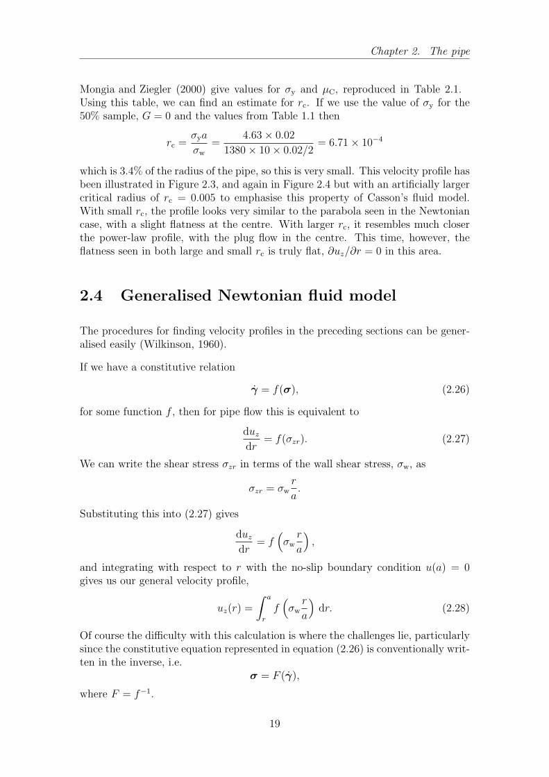
Of course this then reduces equation (3.63) to the 2D equivalent of (3.37), which hasbeen plotted in Figure 3.5 (in orange). Leslie et al. (2011) have found and plottednumerical solutions for B, V 6= 0 (reproduced here in Figure 3.7) and also discussthe cases of B → ∞, V → 0, V → −∞ for further reading.

39

MATHM901 The fluid dynamics of chocolate fountains

Figure 3.7: Film thickness h against θ for differing values of B and V , computed usingnumerical methods. Source: Leslie et al. (2011)

40

Chapter 4

The falling sheet

Flows in liquid sheets with two free surfaces are considerably harder to describethan film flows over solids with only one free surface. The complication lies in threeproperties:

1. two free boundaries,

2. the relation between sheet thickness and distance along the sheet is unknown,

3. the position of the sheet’s trajectory in space is also unknown.

Flows in sheets are nearly irrotational or extensional since both boundaries of thefluid have no shear upon them, and hence velocity and stress in the streamwisedirection does not vary significantly over the sheet cross-section. Viscous effectsin the sheet then mainly come from the normal stress difference. We will look forsteady flows, but more complications in falling sheets come from their naturallyunsteady nature, and how/when they break up.

Furthermore, in our study, the flow is complicated by the shape of the base of thedome, which curves inwards (see Figure 4.11). We will take a look at the differentphenomena in effect on the falling sheet.

4.1 Inviscid model

Chocolate fountains exhibit behaviour where the falling sheet actually falls in-wards instead of straight down (see Figure 4.1). Extensive work, starting withTaylor and Howarth (1959), has been conducted on water bells, such as in Figure4.2, where a jet of water is impacted onto a flat surface (or two jets impacted intoeach other), and the water spreads out in a thin sheet: essentially it is the water-hitting-a-spoon effect which is undesirable when washing up! Surface tension, as weshall see shortly, then pulls the sheet back inwards to form a closed water bell. We

41

MATHM901 The fluid dynamics of chocolate fountains

Figure 4.1: In the chocolate fountain we can see clearly that the sheet falls inwardsonce it has left the dome.

are interested in the mathematics of how the surface tension pulls the axisymmetricsheet back in, since this inward-falling effect is observed in our chocolate fountain.

We proceed by constructing a force balance at right-angles to the stream using themethod of Button (2005), hence overcoming the first problem by choosing coordin-ates which follow the falling sheet’s path.

We start by setting up the geometry of the falling sheet problem with cylindricalcoordinates (r, θ, z). Since the fluid falls from the dome under gravity, we set our zto be pointing downwards; and we assume the flow to be axisymmetric about thevertical and so consider a ‘slice’ of the falling sheet in the (r, z) plane, Figure 4.3.We also define local coordinates along and normal to the sheet, s, n so that u = us.We define the angle φ to be the small angle between the vertical and the sheet, asshown in Figure 4.3.

We consider a fluid element of length dx, width dy and thickness h, as in Figure4.4. This element has two principal radii of curvature: the axisymmetric, RA, andthe meridian, RM , radii, as shown in Figure 4.5. We assume the element is smallenough to approximate the thickness h to be constant within the element. We nowconsider the forces acting on this element:

1. The force due to gravity acting on the element is

Fg = ρgh(cosφ s+ sinφ n)dxdy.

2. The pressure force caused by the difference between the internal and externalpressures, δp, is

Fp = −δp dx dy n.

3. The force due to surface tension is given by

Fs = 2γs dx dy

(1

RA

+1

RM

)n.

42

Chapter 4. The falling sheet

Figure 4.2: A water bell in action. Two jets, approximately 3mm in diameter with thetop jet slightly larger, collide and form a thin spreading sheet of water.Surface tension pulls the sheet inwards until it forms a closed water bell.Photo by John Huang and John Lienhard; source: Huang and Lienhard(1966).

Figure 4.3: Setup of the geometry of our problem; adapted from Button (2005).

Figure 4.4: We consider a fluid element of length dx, width dy and thickness h;adapted from Button (2005).

43

MATHM901 The fluid dynamics of chocolate fountains

Figure 4.5: The fluid element has two principal radii of curvature, RA and RM . Thecircle for which RA is the radius is in the plane normal to the page.

This is since if we take the surface tension γs to be constant along the surface,then immediately the tangential component of the surface force disappearsby symmetry. Noting that there are two surfaces present, the force in theaxisymmetric direction of curvature becomes 2γs dxdy

RA

n and similarly in the

meridian direction the force is 2γs dxdyRM

n. We add these together to give ourresult above.

We balance these forces by the centripetal acceleration experienced by the fluidparticle towards the vertical pipe at any point on the meridian section. This accel-eration is u2

RM

n.

Taking the normal components of the forces and acceleration, and dividing throughby xy, Newton’s second law gives us

2γs

(1

RA

+1

RM

)+ ρgh sinφ− δp =

ρhu2

RM

(4.1)

where ρhxy is the mass of the fluid element which appears on the right-hand-side.We now substitute the geometric identities

RA =r

cosφ

1

RM

= −dφ

ds

into equation (4.1) and we get

2γs

(cosφ

r− dφ

ds

)+ ρgh sinφ− δp+ ρhu2

dφ

ds= 0. (4.2)

We now consider a flow rate argument. Looking down the z-axis, cross-sections ofthe falling sheets are circles of radius rout and rin. If we say that the position of the

44

Chapter 4. The falling sheet

sheet is r = 12(rout − rin), then the thickness of the sheet is h(z) = rout − rin. If the

flow rate is constant at Q, then by continuity, for all z we have

Q =[πr2out(z)− πr2in(z)

]u(z)

= 2πrh(z)u(z)

=⇒ h(z) =Q

2πru

Which if we substitute into our value of h in (4.2), we get

2γs

(cosφ

r− dφ

ds

)+Qρg sinφ

2πru− δp+

ρQu2

2πru

dφ

ds= 0. (4.3)

We now non-dimensionalise our variables by scaling in the following way:

z =z

Lr =

r

Ls =

s

Lu =

u

u0

where u0 is our initial velocity as it leaves the dome and

L =ρQu04πγs

.

Using values from Table 1.1 and the same flux Q as in Figure 3.5, L ≈ 2 cm, whichis roughly how far our fluid falls inwards in experiment, so this is a sensible choicefor us to scale our falling sheet on. This scaling in equation (4.3) gives

cosφ

r− dφ

ds− α + β

sinφ

ur+u

r

dφ

ds= 0 (4.4)

where

α =ρQu0δp

8πγ2sβ =

ρgQ

4πγsu0.

We choose this form of the equation since it is clearer than equation (4.4), andhence our falling sheet, only depends on the parameters α and β. The parameter αaccounts for the effect of the inside-outside pressure difference δp, and β accountsfor gravity.

We are seeking an equation for r as a function of z, r = r(z). We now take allvariables to be dimensionless as we omit the hats for convenience. Equation (4.4)then becomes

cosφ

r− dφ

ds

(ur− 1

)− α + β

sinφ

ur= 0 (4.5)

which, if we then notice that r′(z) = tanφ, this gives us

1

cosφ=

(1 + r′2

)1/2 dφ

ds= r′′ cos3 φ (4.6)

and if we substitute this into equation (4.5) we get the final governing equation forthe shape of the falling sheet:

r′′(u− r) +(1 + r′2

)(1 +

β

ur′)− αr

(1 + r′2

)3/2= 0 (4.7)

45

MATHM901 The fluid dynamics of chocolate fountains

with the initial conditions∗

r(0) = R/L, r′(0) = 0 (4.8)

Now we want to work out the speed u as a function of z and to do this we needto use the inviscid approximation. We assume that the sheet is thin enough thatwe can assume to the velocity to be constant through a cross-section at a givenz. Since the surface of the liquid film is itself a streamline, we can use Bernoulli’s(dimensional) equation for any arbitrary point along a streamline where gravity isconstant:

1

2u2 − gz +

p

ρ= const.

The streamline is also a free surface, so the pressure p is constant, and hence p/ρis constant. The equation then reduces to

u2 − 2gz = const.

How good this inviscid approximation is, is difficult to determine exactly withoutbeing able to measure the speed of the flow reliably throughout its fall. Brunet et al.(2004) use a silicon oil with similar densities and surface tension to chocolate (ρ =970 kgm−3, γs = 0.0204Nm−1) but smaller (but considerably higher than water)viscosity of 0.2Pa s. They were able to measure the speed of the flow as it falls,and plotting the squared speed u2 against z, the results were generally along theline u2 = 2gz. Chocolate, of course, is much more viscous, and we will discuss thismore later.

Since u = u0 at z = 0 when the fluid leaves the dome,

u2 = u20 + 2gz, (4.9)

which if we non-dimensionalise as before, becomes

u2 = 1 + 2βz. (4.10)

We then are left with the complete governing equations (4.7), (4.8) and (4.10) tosolve. Analytically this is only possible where α = β = 0. Although we say laterthat α = 0, since we don’t expect any significant pressure difference δp between theinside and outside of the sheet, we cannot say this for β, since this term representsgravity terms, and the Froude number (U/

√gR), which represents the ratio of

inertial to gravitational forces, is order 1. So we will use the scaling argumentsgiven in Button (2005) and reproduced below.

If we take equation (4.2) and substitute the φ terms for those in equation (4.6)(which come from Y ′(z) = tanφ), we get

2γsr(1 + r′2)1/2

− 2γsr′′

(1 + r′2)3/2+

ρghr′

(1 + r′2)1/2− δp+

ρhu2r′′

(1 + r′2)3/2= 0. (4.11)

∗If we look at Figure 4.1, we can see that the sheet does not fall directly downwards, i.e.r′(0) < 0. We could of course measure the angle here and work out which value of r′(0) we wantto set as the initial condition, but for sake of argument let’s assume ideally that the sheet leavesthe dome vertically.

46

Chapter 4. The falling sheet

We scale r like R = R/L, the scaled radius of the sphere. Now, in this model, whenthe fluid leaves the dome, the fluid falls under gravity, and we will assume the flow isdominated by gravity rather than surface tension. If the fluid is left to fall withoutthe presence of either another dome beneath it or the reservoir at the bottom, thenthe sheet should fall a long distance Z, where Z > R but Z2 ≫ R2. If we performscaling analysis on equation (4.11) in this way and then multiply through by R, wefind that it scales as

2γs(1 +

(RZ

))1/2 − 2γs(RZ

)2(1 +

(RZ

)2)3/2+

ρghR(RZ

)(1 +

(RZ

)2)1/2− δpR+

ρhu2(RZ

)2(1 +

(RZ

)2)3/2∼ 0.

Since (R/Z)2 ≪ 1, this equation, where we have divided through by R, reduces to

2γsR +

ρghRZ − δp ∼ 0,

which represents1

r+ β

r′

r− α = 0

from equation (4.11).

We now argue that the pressure difference between the inside and the outside of thesheet is zero, since the sheet in reality is not continuous enough to form a properseal. So α = 0 and hence equation (4.11) reduces to

r′(z) = −uβ, (4.12)

and substituting in equation (4.10),

r′(z) = −(1 + 2βz)1/2

β.

Which, when integrated with the boundary condition r(0) = R/L (remember z hasbeen scaled here), produces an equation for r,

r(z) =R

L+

1− (1 + 2βz)3/2

3β2. (4.13)

This equation (in dimensional form) has been plotted in Figure 4.6, with datafrom Table 1.1. We can see that it captures the essence of what we see in thefalling sheet, photographed in Figure 4.1, and shows the sheet falling inwards dueto surface tension with slope of the same order we expect. However, this modeldoes not match in all the right places. Firstly, it predicts that the sheet falls inabout 3 cm over the 7 cm drop, when we observe in experiment only about half that.Secondly, we can see in Figure 4.1 that the falling sheet does not start by fallingdirectly down—it falls from the beginning at a slant, and we have lost the abilityto set r′(0) in doing this scaling analysis which reduces the order of the governingequation. We will shortly go on to explain the other effects at work here.

47

MATHM901 The fluid dynamics of chocolate fountains

0.010.02

0.030.04

0.050.06

0.07-

z

0.045

0.050

0.055

0.060

0.065

0.070

r

Figure 4.6: Plot of the dimensionalised form of equation (4.13) with values from Table1.1. We can see that this produces a shape which captures of the essenceof what we see, but falls too far inwards.

4.1.1 Validity of inviscid approximation

Viscous effects are expected to play a part here, as shown by the following calcu-lation. We will compare the energy used in the work done by viscous forces in thefalling fluid, K, with the total energy coming in from the previous stage, E, andshow that viscous effects should be apparent in our analysis of the falling sheet.

Cauchy’s energy equation for energy K in a viscous Newtonian fluid of volume Vand viscosity µ is, generally,

dK

dt= −

∫

V

2µγij γij dV (4.14)

where γij is the ijth component of our rate of strain tensor γ. But

γij =1

2

(∂ui∂xj

+∂uj∂xi

)(4.15)

in coordinates (x1, x2, x3) with respective velocities (u1, u2, u3).

We have worked out from our geometry in equation (4.9) that, in dimensionalisedform,

u2 = u20 + 2gz

in m s−1. Hencedu

dz=

g

(u20 + 2gz)1/2(4.16)

48

Chapter 4. The falling sheet

in s−1. Now the velocity is predominantly vertical, and so we say that the dominantrate of strain tensor is γ33, if we briefly use Cartesian coordinates (x, y, z) with aninverted z component. Hence, plugging equation (4.16) into equation (4.15) we get

γ33 =g

(u20 + 2gz)1/2

in s−1. Now the fluid is incompressible (∇·u = 0) and so γ is traceless (∑

i γii = 0).Hence at best, γ11 = γ22 = −1

2γ33 or at worst, γ11 = −γ33 and γ22 = 0. Taking the

best-case scenario and substituting into equation (4.14) we get

dK

dt= −

∫

V

3µg2

u20 + 2gzdV

= −3µg2∫

V

1

u20 + 2gzdz · xy

= −3

2µg

[log(2gz + u20)

]ℓ0· xy

= −3

2µg log

(2gℓ

u20+ 1

)· xy (4.17)

in J s−1, where xy is∫dx dy and ℓ is the height of the drop.

Compare this to the kinetic energy EK entering the system

EK =1

2ρ

∫

V

u2 dV

=1

2ρ

∫ ℓ

0

(u20 + 2gz

)dz · xy

=1

2ρ(u20ℓ+ gℓ2

)· xy

in Joules, and the potential energy difference EP of the system at the top andbottom

EP =

∫ ℓ

0

ρgz dz · xy

= ρgℓ2

2· xy

also in Joules.

Substituting our values from Table 1.1 into these equations, we find that in a fifthof a second, an estimate for how long it takes chocolate to complete its fall, theenergy absorbed by viscous forces K is equal to 208xy J. The combined kinetic andpotential energy entering the sheet from the dome is E = EK + EP = 101xy J. Sowe see that the viscous forces are expected to contribute highly.

49

MATHM901 The fluid dynamics of chocolate fountains

0.01 0.02 0.03 0.04 0.05 0.06 0.07z

0.05

0.10

0.15

0.20

u

Figure 4.7: Plot of dimensionalised velocity of the sheet as a function of z in the invis-cid (blue, equation 4.10) and viscous (pink, equation 4.18, µ = 10Pa s)cases.

4.2 Viscous model

Gilio et al. (2005) examine 2D falling nonsteady liquid sheets, deriving governingequations through a different (and newer, but less intuitive) method, and discussesviscous effects at the end. The viscous equations are solved numerically using finite-difference methods, and the results are interesting and relevant to our falling sheetof chocolate.

Figure 4.7 plots the velocity of the sheet as a function of z in the inviscid andviscous cases. The inviscid plot is equation (4.10), derived by us. Gilio et al. (2005)give results for both their inviscid and viscous (where they have used a fluid withviscosity 10Pa s, close to our chocolate value of 14Pa s) cases, and we have matchedour inviscid graph with theirs to find the equation governing the viscous velocity,which is remarkably linear and is given in non-dimensional form by

u(z) = 1 + 2.12z. (4.18)

We can substitute this velocity into equation (4.12) to find an equation governingthe position of the viscous sheet in time, namely

r(z) =R

L− z + 1.06z2

β, (4.19)

recalling that these equations are still nondimensional. This has been plotted (indimensional form) in Figure 4.8, alongside the inviscid case for comparison. Whatwe see in this plot is that the viscous sheet does not fall as far inwards as in theinviscid prediction, instead only falling about 1.5 cm inwards over the 7 cm drop:this very closely matches what we observe in running the chocolate fountain.

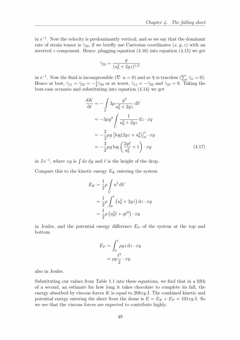
Figure 4.9 shows the profile of the falling sheets in the inviscid and viscous cases forartificially lower and higher surface tensions than that given (and used in Figure4.8) for chocolate. Predictably, higher surface tensions bring the sheet in further.Interestingly, it affects the viscous sheet more than the inviscid sheet, with the

50

Chapter 4. The falling sheet

0.010.02

0.030.04

0.050.06

0.07-

z

0.045

0.050

0.055

0.060

0.065

0.070

r

Figure 4.8: Profile of the falling sheet from the equations derived in the inviscid (blue,equation 4.13) and viscous (pink, equation 4.19, µ = 10Pa s) cases. Theinviscid case is the same as Figure 4.6, and the viscous case has beenmatched from the results in Gilio et al. (2005).

viscous sheet falling further inwards in the higher surface tension case than theinviscid prediction.

4.3 The teapot effect

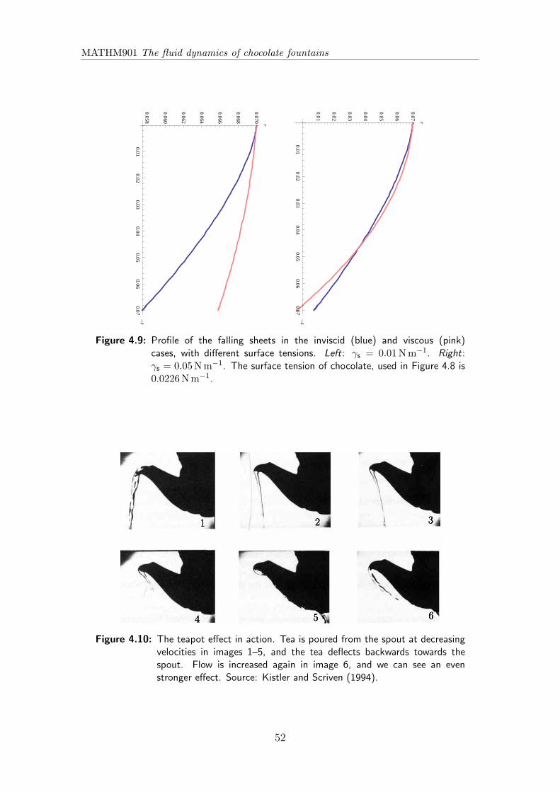
The so-called ‘teapot effect’ was first written about in Reiner (1956), where theterm was coined. The effect is an everyday occurrence and is shown in Figure4.10: when pouring tea from a teapot at fairly slow speeds, the tea has a tendencyto curve backwards and dribble down the spout instead of falling nicely into thecup. The relevance to our chocolate fountain problem is that, as shown in Figure4.11, the dome from which the chocolate falls is curved at the edge, which is aproperty of badly-formed teapots. Of course, in teapots, this falling backwards isnot a phenomenon that we want, although in a chocolate fountain, we do wantthis because it produces the aesthetic of the inward-falling sheet. Considerablework has been done on the teapot effect, summarised nicely in the introduction ofKistler and Scriven (1994), and here we discuss just a few of the explanations.

The analogy is not full, though, since we have no spout and the dome is hollow. Theteapot effect is not 3D and axisymmetric, however, Kistler (1983) derives governingequations for an axisymmetric viscous falling sheet in the same manner as the 2D‘teapot’ case. The physics responsible for the teapot effect is however relevant toboth the teapot and our fountain, so we shall entertain the teapot effect for a fewparagraphs.

51

MATHM901 The fluid dynamics of chocolate fountains

0.010.02

0.030.04

0.050.06

0.07-

z0.058

0.060

0.062

0.064

0.066

0.068

0.070

r

0.010.02

0.030.04

0.050.06

0.07-

z

0.01

0.02

0.03

0.04

0.05

0.06

0.07

r

Figure 4.9: Profile of the falling sheets in the inviscid (blue) and viscous (pink)cases, with different surface tensions. Left: γs = 0.01Nm−1. Right:γs = 0.05Nm−1. The surface tension of chocolate, used in Figure 4.8 is0.0226Nm−1.

Figure 4.10: The teapot effect in action. Tea is poured from the spout at decreasingvelocities in images 1–5, and the tea deflects backwards towards thespout. Flow is increased again in image 6, and we can see an evenstronger effect. Source: Kistler and Scriven (1994).

52

Chapter 4. The falling sheet

Figure 4.11: Relevance of the teapot effect to our chocolate fountain. The edge ofthe dome, from which the chocolate falls, is curved, emphasised by thearrow.

Figure 4.12: What we see when we pour liquid down a slope is that the liquid creepsupwards instead of falling entirely downwards. This contributes to aninwards-falling sheet. Adapted from Kistler and Scriven (1994).

53

MATHM901 The fluid dynamics of chocolate fountains

Figure 4.13: Reiner’s first hypothesis for the teapot effect. ‘Vortices’ are created alongthe fluid path due to the velocity profile, which pushes the fluid towardsthe underside of the body it is flowing around. Adapted from Reiner(1956).

Figure 4.12 shows diagrammatically what we see when we pour liquid down a slopebefore it falls off: the fluid creeps upwards before falling down. Surface tension isresponsible, as we saw in Section 4.1, for the sheet falling inwards. However, it isnot, as Reiner writes, surface tension which is responsible for this creep effect.

Reiner makes two observations about the fluid continuing to move backwards, thefirst of which he offers an explanation for, which we will mention. Figure 4.13 showsthis: that ‘vortices’ are created along the fluid path due to the velocity profile, whichpushes the fluid towards the underside of the body as it flows around.

Keller (1957) gives a different explanation, quoted here:

Qualitatively the explanation is this. When the liquid flows around thelip its velocity is greatest at the lip. By Bernoulli’s principle the pressureis then lowest there. Consequently the surrounding air or other fluidpushes the liquid against the lip by virtue of its atmospheric pressure.This enables the flow to turn the corner. Once the flow has turned thecorner it continues along the underside of the spout rather than fallingbecause the surrounding air supports it. This upside-down flow, althoughunstable, will travel quite far down the spout before its instability resultsin detachment, if the liquid layer is thin. When detachment occurs thejet will fall backwards since its velocity is directed away from the lip.

This explanation is supported with mathematical work considering 2D flow of in-viscid, incompressible fluid leaving a horizontal spout. Once again, we see that theviscosity of the fluid is not a cause of deflection in the flow.

54

Chapter 4. The falling sheet

Figure 4.14: Applying a super-hydrophobic coating to the spout reduces the teapoteffect in experiment. Source: Duez et al. (2009).

Duez et al. (2009) argue that surface wettability is an important factor, follow-ing experiment. They argue that coating the spout of the teapot with a super-hydrophobic surface avoids the teapot effect altogether, as shown in Figure 4.14.Of course, in the chocolate fountain, this could be useful information: to maximisethe teapot effect to produce inwards-falling sheets, one should wet the undersidesof the domes first. This conclusion seems to contradict that of Reiner, who saysthat coating the spout with some water-repelling material didn’t make any differ-ence, hence suggesting that surface tension plays very little part in the dynamicsof the fluid. It cannot be argued that such super-hydrophobic materials as used byDuez et al. were not invented: in Figure 4.14 they have coated the teapots withblack soot, which would have been more prevalent in the time of Reiner.

Ultimately the teapot effect is a complicated phenomenon which is, due to time,beyond the scope of this project to investigate fully. I have only briefly discussedthe physics behind various studies but more rigorous and full analysis could be aproject of its own, particularly since it involves considerable numerical work.

4.4 Concluding remarks on the falling sheet

The falling sheet is a difficult problem because there are a number of differentphenomena acting together. The teapot effect showcases some of these quite nicely.We were able to solve for an inviscid falling sheet by simplifying the problem, butviscous falling sheets require numerical work which, due to time constraints, wehave not been able to undertake. Relevant published papers that have performedthis work have been mentioned.

55

56

Bibliography

J.-M. Aeschlimann and S. T. Beckett. International interlaboratory trials to de-termine the factors affecting the measurement of chocolate viscosity. Journalof Texture Studies, 31(5):541–576, November 2000. ISSN 1745-4603. doi:10.1111/j.1745-4603.2000.tb01019.x. URL http://onlinelibrary.wiley.com/

doi/10.1111/j.1745-4603.2000.tb01019.x/abstract.

Emmanuel Ohene Afoakwa, Alistair Paterson, Mark Fowler, and Joselio Vieira.Comparison of rheological models for determining dark chocolate viscosity. In-ternational Journal of Food Science & Technology, 44(1):162–167, January 2009.ISSN 09505423, 13652621. doi: 10.1111/j.1365-2621.2008.01710.x. URL http://

strathprints.strath.ac.uk/16013/.

N. J. Balmforth and R. V. Craster. Dynamics of cooling domes of visco-plastic fluid. Journal of Fluid Mechanics, 422:225–248, November 2000. ISSN00221120. URL http://resolver.scholarsportal.info/resolve/00221120/

v422inone/225_docdovf.xml.

Jrgen Blumm and Andr Lindemann. Characterization of the thermophys-ical properties of molten polymers and liquids using the flash technique.High Temperatures - High Pressures, 35/36(6):627–632, 2003. doi: 10.1068/htjr144. URL http://thermophysics.ru/pdf_doc/AutoPlay/Docs/

CollectionOfManuscripts/ECTP2005paper104.pdf.

P. Brunet, C. Clanet, and L. Limat. Transonic liquid bells. Physics of Fluids, 16(7):2668, 2004. ISSN 10706631. doi: 10.1063/1.1738650. URL http://link.

aip.org/link/PHFLE6/v16/i7/p2668/s1&Agg=doi.

Eleanor C. Button. The dynamics of water bells. Honours thesis, University ofMelbourne, Mathematics & Statistics, November 2005. URL http://www.ms.

unimelb.edu.au/publications/button.pdf.

N. Casson. A flow equation for pigment-oil suspensions of the printing ink type.In C. C. Mill, editor, Rheology of disperse systems: Proceedings of a conferenceorganized by the British Society of Rheology and held at the University College ofSwansea in September 1957. Pergamon Press, 1959.

C. R. Daubert, J. F. Steffe, and J. R. Lloyd. Electric field effects on the thermal con-ductivity of milk chocolate determined using the mirror image method. Journal

57

MATHM901 The fluid dynamics of chocolate fountains

of Food Process Engineering, 20(1):77–89, February 1997. ISSN 1745-4530. doi:10.1111/j.1745-4530.1997.tb00412.x. URL http://onlinelibrary.wiley.com.

libproxy.ucl.ac.uk/doi/10.1111/j.1745-4530.1997.tb00412.x/abstract.

C. Duez, C. Ybert, C. Clanet, and L. Bocquet. Beating the teapot effect. PhysicalReview Letters, 104:084503, October 2009. URL http://arxiv.org/abs/0910.

3306.

M. Gilio, F. Al-Bender, and J.-P. Kruth. The dynamics of a moving sheet ofliquid, part I: derivation of the 2D equations of motion. European Journalof Mechanics - B/Fluids, 24(5):555–571, October 2005. ISSN 0997-7546.doi: 10.1016/j.euromechflu.2004.12.003. URL http://www.sciencedirect.com/

science/article/pii/S0997754604001311.

C. P. Huang and J. H. Lienhard. The influence of gravity upon the shape of waterbells. Journal of Applied Mechanics, 33(2):457, 1966. ISSN 00218936. doi:10.1115/1.3625072. URL http://adsabs.harvard.edu/abs/1966JAM....33..

457H.

Esther L. Keijbets, Jianshe Chen, Eric Dickinson, and Joselio Vieira. Surfaceenergy investigation of chocolate adhesion to solid mould materials. Journalof Food Engineering, 92(2):217–225, May 2009. ISSN 0260-8774. doi: 10.1016/j.jfoodeng.2008.11.008. URL http://www.sciencedirect.com/science/

article/pii/S026087740800544X.

Joseph B. Keller. Teapot effect. Journal of Applied Physics, 28(8):859–864, August1957. ISSN 00218979. doi: 10.1063/1.1722875. URL http://jap.aip.org.

libproxy.ucl.ac.uk/resource/1/japiau/v28/i8/p859_s1.

S. F. Kistler and L. E. Scriven. The teapot effect: sheet-forming flows with deflec-tion, wetting and hysteresis. Journal of Fluid Mechanics, 263:19–62, 1994. doi:10.1017/S0022112094004027.

Stephan F. Kistler. The fluid mechanics of curtain coating and related viscous freesurface flows with contact lines. PhD thesis, University of Minnesota, November1983.

G. A. Leslie, S. K. Wilson, and B. R. Duffy. Non-isothermal flow of a thin film offluid with temperature-dependent viscosity on a stationary horizontal cylinder.Physics of Fluids, 23(6):062101, 2011. ISSN 10706631. doi: 10.1063/1.3593393.URL http://strathprints.strath.ac.uk/33826/.

Gagan Mongia and Gregory R. Ziegler. The role of particle size distribution ofsuspended solids in defining the flow properties of milk chocolate. Interna-tional Journal of Food Properties, 3(1):137–147, 2000. ISSN 1094-2912. doi:10.1080/10942910009524621. URL http://www.tandfonline.com.libproxy.

ucl.ac.uk/doi/abs/10.1080/10942910009524621.

58

Bibliography

Savina Radosasvljevic, Anna Schlunk, Roger Tanner, and Simin Nasseri. Melt-ing chocolate, February 2000. URL http://web.aeromech.usyd.edu.au/

rheology/snasseri/images/chocolate.pdf.

Markus Reiner. The teapot effect... a problem. Physics Today, 9(9):16, 1956.ISSN 00319228. doi: 10.1063/1.3060089. URL http://www.physicstoday.org/

resource/1/phtoad/v9/i9/p16_s1?isAuthorized=no.

Serpil Sahin and Servit Gulum Sumnu. Physical properties of foods. Springer, 2006.ISBN 9780387307800.

Daisuke Takagi and Herbert E. Huppert. Flow and instability of thinfilms on a cylinder and sphere. Journal of Fluid Mechanics, 647:221, March 2010. ISSN 0022-1120, 1469-7645. doi: 10.1017/S0022112009993818. URL http://65.54.113.26/Publication/26707321/

flow-and-instability-of-thin-films-on-a-cylinder-and-sphere.

Geoffrey Taylor and L. Howarth. The dynamics of thin sheets of fluid. I. Waterbells. Proceedings of the Royal Society of London. Series A. Mathematical andPhysical Sciences, 253(1274):289 –295, December 1959. doi: 10.1098/rspa.1959.0194. URL http://rspa.royalsocietypublishing.org/content/253/1274/

289.abstract.

Sukanya Wichchukit, Michael J. McCarthy, and Kathryn L. McCarthy. Flow be-havior of milk chocolate melt and the application to coating flow. Journal ofFood Science, 70(3):E165–E171, April 2005. ISSN 1750-3841. doi: 10.1111/j.1365-2621.2005.tb07131.x. URL http://onlinelibrary.wiley.com.libproxy.

ucl.ac.uk/doi/10.1111/j.1365-2621.2005.tb07131.x/abstract.

William Lionel Wilkinson. Non-Newtonian fluids: fluid mechanics, mixing and heattransfer. Pergamon Press, 1960.

Klaus Wollny. Determining the yield point and viscosity of chocolate, February2005. URL http://www.mep.net.au/foodlab/FL_7/AN_RLQC_Choco_B.pdf.

59