The Theory of Price Collars: The Linking of Prices in a ...

The Theory of Price Collars: The Linking of Prices in a Market Channel to

Redress the Exercise of Market Power

April 15, 2004

by Li Tian and Ronald W. Cotterill

Food Marketing Policy Center Department of Agricultural and Resource Economics

University of Connecticut Storrs, CT 06269-4021

Tel: (860) 486-2742 Fax: (860) 486-2461

Email: [email protected]

Website: http://www.fmpc.uconn.ed

2

THE THEORY OF PRICE COLLARS: THE LINKING OF PRICES IN A MARKET

CHANNEL TO REDRESS THE EXERCISE OF MARKET POWER

Li Tian and Ronald W. Cotterill

I. Introduction

The marketing channels for many goods involve the production of a raw commodity that is

processed and then distributed to retailers for sale to consumers. Either the processing industry

or the retailing industry or both may exercise substantial market power ultimately against raw

commodity suppliers or consumers, the disorganized (competitive) economic groups at the ends

of the market channel. This paper develops a theory of price collars to regulate pricing in such a

channel. Price collars link raw product, wholesale and retail prices but do not explicitly set such

prices. For example, a wholesale price collar could limit the wholesale price to 140% of the raw

commodity price, and a retail price collar could limit retail price to 130% of the wholesale price.

Note that this policy has 2 instruments that address three prices. Thus the policy cannot

set these prices. This is by design. The policy seeks to preserve a modicum of firm pricing

authority to allow firms to react to cost and demand shifts in the industries. Our theory analyzes

what retail, wholesale and raw commodity prices would be in a post-regulation equilibrium

assuming firms maximize profits. We derive the conditions that must be satisfied to generate an

increase or decrease in each of the three prices in the marketing channel, and show how

equilibrium prices change when a regulatory agency alters the price collars. Although the

agency does not set prices it can manage prices to attain desired policy targets.

This paper is organized as follows: section I is introduction, section II analyzes post-

regulation retail pricing and the implication of retail price leadership for wholesale and raw

product prices. Since wholesale and raw product prices are linked by price collars, we show that

3

retailers also determine those prices when setting retail prices. We derive the qualitative

conditions that are necessary for post-regulation retail, wholesale and raw prices to be higher, the

same, or lower than pre-regulation prices and the formulas for post-regulation equilibrium prices.

Section III analyzes post-regulation wholesale pricing and the implication of wholesale

price leadership for retail and raw product prices. As in the retail pricing section the regulation

links wholesale pricing moves to retail and raw prices. We also derive the formulas for post-

regulation equilibrium prices and qualitative analysis of the difference between pre-and post-

regulation prices.

Section IV recognizes the retailer’s and processor’s profit maximizing moves under

regulation generate different desired equilibrium price vectors. We suggest that under regulation

retailers and processors must bargain and that the resulting equilibrium prices will depend on the

relative bargaining power of retailers and processors.

Section V applies the theory to the fluid milk market in New England where there is

documented market power and excessive margins at the retail. Retailers clearly dominate the

market channel, and our analysis documents that dominance. The intent of a proposed milk price

collar policy in Connecticut is to reduce retail margins by increasing raw (farm) milk prices and

reducing retail prices. Nonetheless the regulatory regime would permit firms to cover their costs

and earn profits, but profits more in line with a competitive rate of return. Section VI concludes

the paper.

II. Pre- and Post-Regulation Prices with Retailer Price Leadership under Regulation

Following Slade (1995) and others we initially assume that each retail firm has a monopoly

based upon geographic location and product differentiation, i.e. the firm’s demand curve for the

4

processed product under analysis is downward sloping. We will relax this assumption to analyze

retail oligopoly pricing of differentiated products. We assume that a supermarket chain applies

category management techniques, i.e. it seeks to maximize the joint profit of all brands it sells in

this category; and we assume that the retail price collar applies to all brands in the processed

product category.

Finally we need specify the nature of vertical competition with processors. Essentially

we assume that retailers regard the wholesale milk prices as a parameter when maximizing

profits. This may be due to one of two possibilities. Processing may be effectively competitive

with a flat supply curve or retailers may play a vertical Nash game, i.e. maintain that their pricing

moves have no effect on a processing oligopoly that feed back through changes in wholesale

price to alter their pricing strategies.

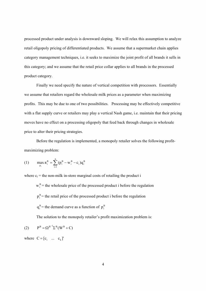
Before the regulation is implemented, a monopoly retailer solves the following profit-

maximizing problem:

(1) Bi

n

1ii

Bi

Bi

Rip

q)cw(pπmaxi

∑=

−−=

where ci = the non-milk in-store marginal costs of retailing the product i

Biw = the wholesale price of the processed product i before the regulation

Bip = the retail price of the processed product i before the regulation

Biq = the demand curve as a function of B

ip

The solution to the monopoly retailer’s profit maximization problem is:

(2) C)(WP BB1BB +ΣΩ=−

where ]'c...c[C ki=

5

+

+=Ω

)ε(1s...εs.........εs...)ε(1s

Bnn

Bn

Bn1

B1

B1n

Bn

B11

B1

B

=ΣBnn

Bn

Bn1

B1

B1n

Bn

B11

B1

B

εs...εs.........εs...εs

Qqs

BiB

i = ; Q is the total quantity for the entire market

Bj

Bi

Bi

BjB

ji qp

pq

ε∂∂

=

After a price collar policy is implemented, the retail price collar, k, is binding because the

policy goal is to lower retail price. A monopoly retailer’s profit maximization problem is now

different. Define a new vector of prices Bi

Bii

Ni wpp)

k11(p −=−= . Now the firm’s retail profit

maximization problem can be restated in Nip as follows:

(3) i

n

1ii

Nii

pq)c(pπmax

iNi

∑=

−=

where iNi p

k1kp −

= . The solution to this new problem when Nip is the new choice variable is:

(4) CP 1N ΣΩ= −

where ]'p...p[P Nn

Ni

N =

+

+=Ω

)ε(1s...εs.........εs...)ε(1s

Nnnn

Nn11

N1nn

N111

6

=ΣNnnn

Nn11

N1nk

N111

εs...εs.........εs...εs

Qqs i

i = ; Q is the total quantity for the entire market

j

Ni

Ni

jNji q

ppq

ε∂∂

=

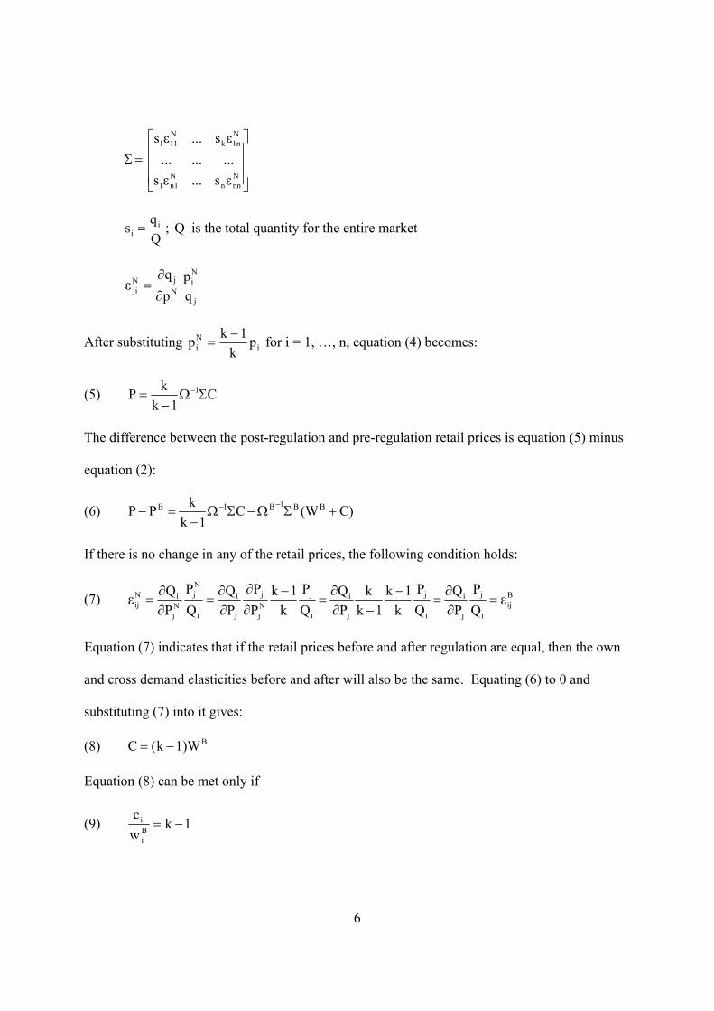
After substituting iNi p

k1kp −

= for i = 1, …, n, equation (4) becomes:

(5) C1k

kP 1ΣΩ−

= −

The difference between the post-regulation and pre-regulation retail prices is equation (5) minus

equation (2):

(6) C)(WC1k

kPP BB1B1B +ΣΩ−ΣΩ−

=−−−

If there is no change in any of the retail prices, the following condition holds:

(7) Bij

i

j

j

i

i

j

j

i

i

jNj

j

j

i

i

Nj

Nj

iNij ε

QP

PQ

QP

k1k

1kk

PQ

QP

k1k

PP

PQ

QP

PQε =

∂∂

=−

−∂∂

=−

∂∂

∂∂

=∂∂

=

Equation (7) indicates that if the retail prices before and after regulation are equal, then the own

and cross demand elasticities before and after will also be the same. Equating (6) to 0 and

substituting (7) into it gives:

(8) B1)Wk(C −=

Equation (8) can be met only if

(9) 1kwc

Bi

i −=

7

for all products, i = 1, …, n. If 1kwc

Bi

i −> , post-regulation retail price is higher. If 1kwc

Bi

i −< ,

post-regulation retail price is lower.

Given that retailers honor the constraint p = kw, the wholesale price and raw milk price

after the regulation is implemented is:

(10) C1k

1W 1ΣΩ−

= −

Assuming the pre-regulation ratio of wholesale and raw price is greater than m, if Bii ww ≥ , then

the post-regulation raw price is also higher. Since processors honor the second price collar, i.e.

w = mr, the raw product price under the retailer leadership case is:

(11) C1)m(k

1R 1ΣΩ−

= −

If one has estimated values of in-store marginal cost and supermarket own price

elasticities of demand then one can simulate the post-regulation equilibrium prices and compare

them to pre-regulation equilibrium prices.

II.1 Generalization to Retail Oligopoly

A more general model of competition among supermarkets chains for shoppers explicitly

incorporates cross–chain substitubility for retail product purchases. We illustrate the implication

of the regulation with the oligopoly case. Assuming general demand function for differentiated

products, a retailer’s profit maximization problem is defined as in equation (1). The only

difference is that the number of brands, n, expands to all brands at different retailers. Assuming

Nash Bertrand pricing among all retailers, we get the following solution for retailer j:

(13) )C(WP jBj

Bj

1Bj

Bj +ΣΩ=

−

8

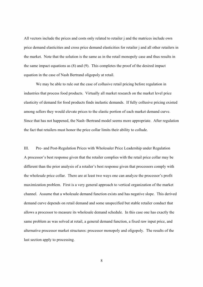
All vectors include the prices and costs only related to retailer j and the matrices include own

price demand elasticities and cross price demand elasticities for retailer j and all other retailers in

the market. Note that the solution is the same as in the retail monopoly case and thus results in

the same impact equations as (8) and (9). This completes the proof of the desired impact

equation in the case of Nash Bertrand oligopoly at retail.

We may be able to rule out the case of collusive retail pricing before regulation in

industries that process food products. Virtually all market research on the market level price

elasticity of demand for food products finds inelastic demands. If fully collusive pricing existed

among sellers they would elevate prices to the elastic portion of each market demand curve.

Since that has not happened, the Nash–Bertrand model seems more appropriate. After regulation

the fact that retailers must honor the price collar limits their ability to collude.

III. Pre- and Post-Regulation Prices with Wholesaler Price Leadership under Regulation

A processor’s best response given that the retailer complies with the retail price collar may be

different than the prior analysis of a retailer’s best response given that processors comply with

the wholesale price collar. There are at least two ways one can analyze the processor’s profit

maximization problem. First is a very general approach to vertical organization of the market

channel. Assume that a wholesale demand function exists and has negative slope. This derived

demand curve depends on retail demand and some unspecified but stable retailer conduct that

allows a processor to measure its wholesale demand schedule. In this case one has exactly the

same problem as was solved at retail, a general demand function, a fixed raw input price, and

alternative processor market structures: processor monopoly and oligopoly. The results of the

last section apply to processing.

9

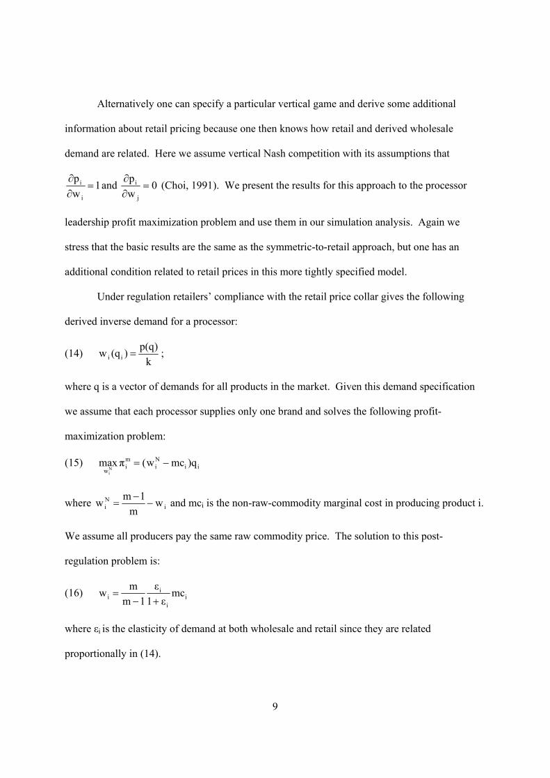
Alternatively one can specify a particular vertical game and derive some additional

information about retail pricing because one then knows how retail and derived wholesale

demand are related. Here we assume vertical Nash competition with its assumptions that

1wp

i

i =∂∂ and 0

wp

j

i =∂∂ (Choi, 1991). We present the results for this approach to the processor

leadership profit maximization problem and use them in our simulation analysis. Again we

stress that the basic results are the same as the symmetric-to-retail approach, but one has an

additional condition related to retail prices in this more tightly specified model.

Under regulation retailers’ compliance with the retail price collar gives the following

derived inverse demand for a processor:

(14) k

)p(q)(qw ii = ;

where q is a vector of demands for all products in the market. Given this demand specification

we assume that each processor supplies only one brand and solves the following profit-

maximization problem:

(15) iiNi

mi

w)qmcw(πmax

Ni

−=

where iNi w

m1mw −

−= and mci is the non-raw-commodity marginal cost in producing product i.

We assume all producers pay the same raw commodity price. The solution to this post-

regulation problem is:

(16) ii

ii mc

ε1ε

1mmw

+−=

where εi is the elasticity of demand at both wholesale and retail since they are related

proportionally in (14).

10

As we know the retailer must comply with the price collar at retail given a pre-determined

wholesale price, the retail price for product i thus must be:

(17) ii

ii mc

ε1ε

1mkmp

+−=

Now let’s state the solution to the processor’s pre-regulation profit maximization

problem:

(18) BiB

ii

BBi

BiB

i gε1

1)mc(rε1

εw+

−++

=

where Biε is the pre-regulation own demand elasticity for processor i, Br is pre-regulation raw

price, imc is the processor i’s marginal cost, and Big is the profit maximizing gross margin at

retail. Adding the retail gross margin to equation (18) gives the pre-regulation profit maximizing

retail price:

(19) BiB

i

Bi

iB

Bi

BiB

iBi

Bi g

ε1ε)mc(r

ε1εgwp

+++

+=+=

In order to examine how wholesale price would change after regulation one needs to

consider the pre- and post-regulation retail prices and corresponding retail demand elasticities.

So let’s first examine the condition for the change in post-regulation retail price. Subtracting

equation (19) from (17) gives:

(20) BiB

i

Bi

iB

Bi

Bi

ii

iBii g

ε1ε)mc(r

ε1εmc

ε1ε

1mkmpp

+−+

+−

+−=−

If there is no change in post-regulation retail price of brand i, then equation (20) is zero and

becomes the following after simplification:

(21) Bii

Bi gmcrmc

1mkm

++=−

or Bi

Bii

Bi wpmcrmc

1mkm

−++=−

11

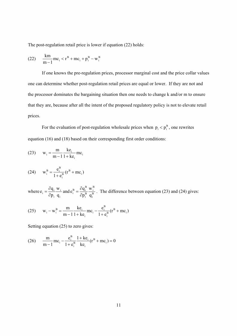
The post-regulation retail price is lower if equation (22) holds:

(22) Bi

Bii

Bi wpmcrmc

1mkm

−++<−

If one knows the pre-regulation prices, processor marginal cost and the price collar values

one can determine whether post-regulation retail prices are equal or lower. If they are not and

the processor dominates the bargaining situation then one needs to change k and/or m to ensure

that they are, because after all the intent of the proposed regulatory policy is not to elevate retail

prices.

For the evaluation of post-regulation wholesale prices when Bii pp < , one rewrites

equation (16) and (18) based on their corresponding first order conditions:

(23) ii

ii mc

ke1ke

1mmw

+−=

(24) )mc(re1

ew iB

Bi

BiB

i ++

=

wherei

i

i

ii q

wpqe∂∂

= and Bi

Bi

Bi

BiB

i qw

pqe∂∂

= . The difference between equation (23) and (24) gives:

(25) )mc(re1

emcke1

ke1m

mww iB

Bi

Bi

ii

iBii +

+−

+−=−

Setting equation (25) to zero gives:

(26) 0)mc(rke

ke1e1

emc1m

mi

B

i

iBi

Bi

i =++

+−

−

12

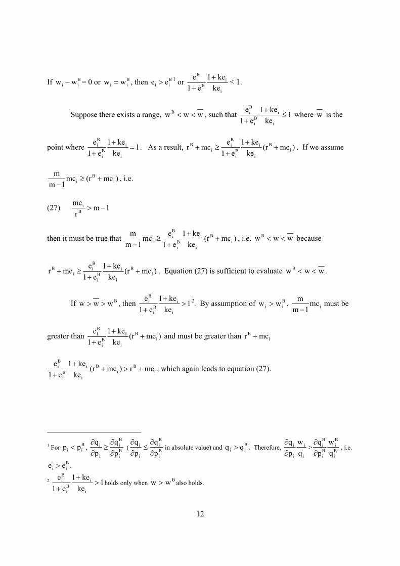
If Bii ww − = 0 or B

ii ww = , then Bii ee > 1 or

i

iBi

Bi

keke1

e1e ++

< 1.

Suppose there exists a range, www B << , such that 1ke

ke1e1

e

i

iBi

Bi ≤

++

where w is the

point where 1ke

ke1e1

e

i

iBi

Bi =

++

. As a result, )mc(rke

ke1e1

emcr iB

i

iBi

Bi

iB +

++

≥+ . If we assume

)mc(rmc1m

mi

Bi +≥

−, i.e.

(27) 1mr

mcB

i −>

then it must be true that )mc(rke

ke1e1

emc1m

mi

B

i

iBi

Bi

i ++

+≥

−, i.e. www B << because

)mc(rke

ke1e1

emcr iB

i

iBi

Bi

iB +

++

≥+ . Equation (27) is sufficient to evaluate www B << .

If Bwww >> , then 1ke

ke1e1

e

i

iBi

Bi >

++

2. By assumption of Bii ww > , imc

1mm−

must be

greater than )mc(rke

ke1e1

ei

B

i

iBi

Bi +

++

and must be greater than iB mcr +

iB

iB

i

iBi

Bi mcr)mc(r

keke1

e1e

+>++

+, which again leads to equation (27).

1 For B

ii pp < , Bi

Bi

i

i

pq

pq

∂∂

≥∂∂

( Bi

Bi

i

i

pq

pq

∂∂

≤∂∂

in absolute value) and Bii qq > . Therefore,

i

i

i

i

qw

pq∂∂

> Bi

Bi

Bi

Bi

qw

pq∂∂

, i.e.

Bii ee > .

2 1ke

ke1e1

e

i

iBi

Bi >

++

holds only when Bww > also holds.

13

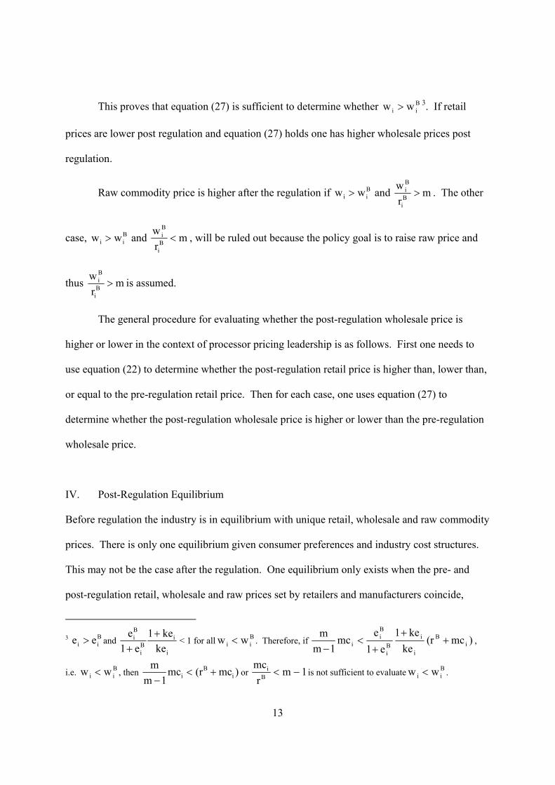
This proves that equation (27) is sufficient to determine whether Bii ww > 3. If retail

prices are lower post regulation and equation (27) holds one has higher wholesale prices post

regulation.

Raw commodity price is higher after the regulation if Bii ww > and m

rw

Bi

Bi > . The other

case, Bii ww > and m

rw

Bi

Bi < , will be ruled out because the policy goal is to raise raw price and

thus mrw

Bi

Bi > is assumed.

The general procedure for evaluating whether the post-regulation wholesale price is

higher or lower in the context of processor pricing leadership is as follows. First one needs to

use equation (22) to determine whether the post-regulation retail price is higher than, lower than,

or equal to the pre-regulation retail price. Then for each case, one uses equation (27) to

determine whether the post-regulation wholesale price is higher or lower than the pre-regulation

wholesale price.

IV. Post-Regulation Equilibrium

Before regulation the industry is in equilibrium with unique retail, wholesale and raw commodity

prices. There is only one equilibrium given consumer preferences and industry cost structures.

This may not be the case after the regulation. One equilibrium only exists when the pre- and

post-regulation retail, wholesale and raw prices set by retailers and manufacturers coincide,

3 B

ii ee > and i

iBi

Bi

keke1

e1e ++

< 1 for all Bii ww < . Therefore, if )mc(r

keke1

e1e

mc1m

mi

B

i

iBi

Bi

i ++

+<

−,

i.e. Bii ww < , then )mc(rmc

1mm

iB

i +<−

or 1mr

mcB

i −< is not sufficient to evaluate Bii ww < .

14

which is unlikely. Retailers and manufacturers most likely will need to engage in some type of

bargaining to find an equilibrium after the regulation.

The bargained equilibrium will lie within intervals: H*L ppp << and H*L www << ,

H*L rrr << where the superscripts L and H stand for high and low and * stands for the post-

regulation bargained equilibrium. The bounds in these intervals are set by the retailer and

processor solutions of the prior two sections. Either the retailer or processor will prefer the high

price vector and the other will prefer the low price vector. If either a retailer or processor is

dominant in the market channel, the equilibrium will be closer to its end of the range of possible

price vectors.

V. Application of the Model to the Southern New England Milk Market

The general theory of price collars can serve any regulatory agency that seeks to restructure raw,

wholesale, and retail prices in a commodity marketing channel for any reason. In this section we

apply the theory to a non-competitive marketing channel. Research on the milk channel in

southern New England gives retail, wholesale and raw milk price and processor marginal cost

(Cotterill, 2003). Data are available for each of the major brands for each supermarket chain;

however in this paper we will analyze the aggregate of “all milk” data for the representative

supermarket and processor to illustrate the theory.

Farmers received $1 per gallon for fluid milk, processing marginal cost was 45 cents per

gallon and processors’ gross margin was 60 cents for a wholesale price of $1.60. This gross

margin is effectively marginal cost plus a competitive return to overhead. The retail price was

$3.10 per gallon.4 Moreover Criner has estimated for the Maine Milk Commission that the in-

4 Prices are rounded to the nearest dime in this illustrative example.

15

store marginal cost for supermarkets is 20 cents (Maine Milk Commission). Others estimate that

a full cost measure, i.e. also covering fixed overhead for supermarkets is 33 to 44 cents per

gallon (Huff, 4/17/03, p.23) and 40 cents per gallon (PMMB, p.17). This means that the net

profit margin in southern New England supermarkets is approximately $1.10 per gallon. This is

an excessive rate of return that has triggered investigation by the Connecticut Attorney General,

legislative hearings in Connecticut and Massachusetts and calls for milk price regulation

including price collar regulation5.

In Connecticut the proposed price collar law would allow a milk regulation board to set

price collars. To date the debate has centered on a k = 1.3 retail price collar and a m = 1.4

wholesale price collar.6 The intent of these price collars is to raise raw (farm) fluid milk prices

and cut retail fluid milk prices to reduce the excessive retail margin without forcing losses on

either retailers or processors. To determine whether the collars will do so and to explore how

changes in the price collar values influence equilibrium prices we start by analyzing the retailer

and processor leadership models. First we will check the qualitative results to see if post

regulation retail prices are lower, and wholesale and process prices are higher in the retailer and

processor leadership models. Then we will simulate the post-regulation price vector for each

model, evaluate the bargaining solution, and determine how the final price solution vector

changes when the Board changes price collar values. This exercise illustrates how the Board can

attain desired target price outcomes.

For the retail leadership model the retail-pricing rule (9) predicts that if the non-milk

marginal cost per gallon of selling milk is less than 30% of the pre-regulation wholesale price

($1.63), i.e. less than 48 cents, then retail price will drop. It is approximately 40-45 cents per

5 See our website http://www.fmpc.uconn.edu. Click on Milk Price Gouging for documentation. 6 See Richard Blumenthal, Connecticut Attorney General, letter to Representative George Wilber, dated January 26, 2004 and the attached draft law http://www.fmpc.uconn.edu. Click on Milk Price Gouging.

16

gallon so retail price is predicted to decline. Since 3.1wp

Bi

Bi > wholesale prices are higher, and

since

4.1rw

B

Bi > raw prices are also predicted to be higher. Given industry cost and pre-regulation

price conditions under retailer leadership model the proposed price collars do move prices in

desired or targeted directions.

For the wholesale price leadership model equation (22) in fact holds for we have:

Bi

Bii

Bi wpmcr60.13.100.451.000.45

4.04.1*3.1mc

1mkm

−++=−++<=−

or 2.0475 < 2.95

This implies that in the processor leadership case retail price will also decline. The relevant

condition to determine how wholesale price will change given retail prices declines is equation

(27):

1m0.4 or00.1

0.45r

mcB

i −=><=

and one has 0.45 > 0.4. Therefore post-regulation wholesale prices are higher than pre-

regulation prices and since:

40.14.1

60.1rw

B

Bi >=

also holds, raw prices are also higher. In conclusion under the processor leadership model the

proposed price collar also move the prices in the desired or targeted direction. Turning now to

the simulation results for the retailer leadership model. The pricing rule for simulating the retail

price of a single product is:

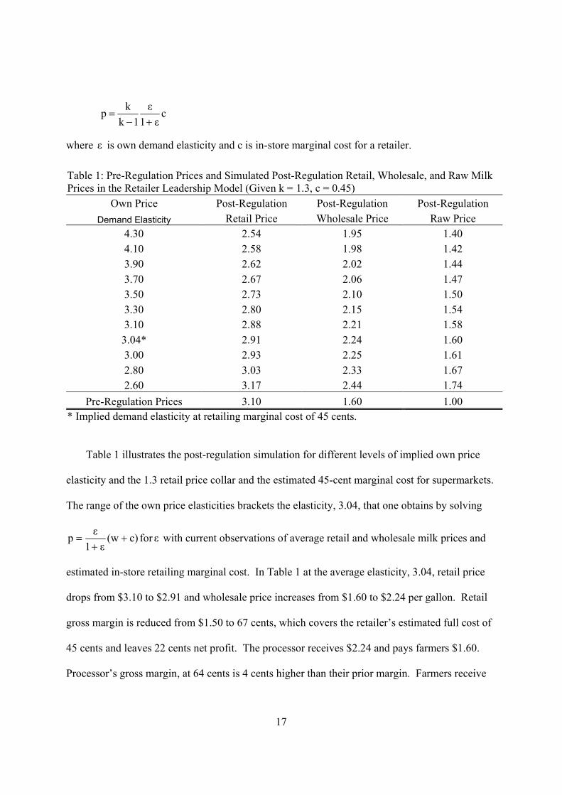
17

cε1

ε1k

kp+−

=

where ε is own demand elasticity and c is in-store marginal cost for a retailer.

Table 1 illustrates the post-regulation simulation for different levels of implied own price

elasticity and the 1.3 retail price collar and the estimated 45-cent marginal cost for supermarkets.

The range of the own price elasticities brackets the elasticity, 3.04, that one obtains by solving

c)(wε1

εp ++

= for ε with current observations of average retail and wholesale milk prices and

estimated in-store retailing marginal cost. In Table 1 at the average elasticity, 3.04, retail price

drops from $3.10 to $2.91 and wholesale price increases from $1.60 to $2.24 per gallon. Retail

gross margin is reduced from $1.50 to 67 cents, which covers the retailer’s estimated full cost of

45 cents and leaves 22 cents net profit. The processor receives $2.24 and pays farmers $1.60.

Processor’s gross margin, at 64 cents is 4 cents higher than their prior margin. Farmers receive

Table 1: Pre-Regulation Prices and Simulated Post-Regulation Retail, Wholesale, and Raw Milk Prices in the Retailer Leadership Model (Given k = 1.3, c = 0.45)

Own Price Post-Regulation Post-Regulation Post-Regulation Demand Elasticity Retail Price Wholesale Price Raw Price

4.30 2.54 1.95 1.40 4.10 2.58 1.98 1.42 3.90 2.62 2.02 1.44 3.70 2.67 2.06 1.47 3.50 2.73 2.10 1.50 3.30 2.80 2.15 1.54 3.10 2.88 2.21 1.58

3.04* 2.91 2.24 1.60 3.00 2.93 2.25 1.61 2.80 3.03 2.33 1.67 2.60 3.17 2.44 1.74

Pre-Regulation Prices 3.10 1.60 1.00 * Implied demand elasticity at retailing marginal cost of 45 cents.

18

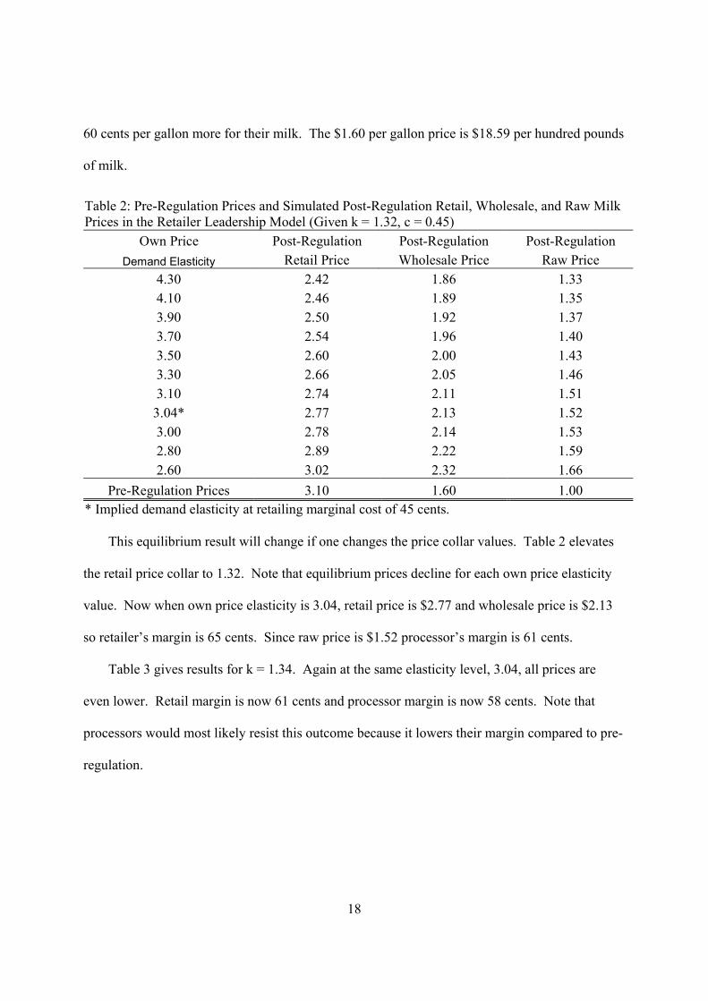
60 cents per gallon more for their milk. The $1.60 per gallon price is $18.59 per hundred pounds

of milk.

This equilibrium result will change if one changes the price collar values. Table 2 elevates

the retail price collar to 1.32. Note that equilibrium prices decline for each own price elasticity

value. Now when own price elasticity is 3.04, retail price is $2.77 and wholesale price is $2.13

so retailer’s margin is 65 cents. Since raw price is $1.52 processor’s margin is 61 cents.

Table 3 gives results for k = 1.34. Again at the same elasticity level, 3.04, all prices are

even lower. Retail margin is now 61 cents and processor margin is now 58 cents. Note that

processors would most likely resist this outcome because it lowers their margin compared to pre-

regulation.



4.30 2.42 1.86 1.33 4.10 2.46 1.89 1.35 3.90 2.50 1.92 1.37 3.70 2.54 1.96 1.40 3.50 2.60 2.00 1.43 3.30 2.66 2.05 1.46 3.10 2.74 2.11 1.51

3.04* 2.77 2.13 1.52 3.00 2.78 2.14 1.53 2.80 2.89 2.22 1.59 2.60 3.02 2.32 1.66


19

Turning now to the processor leadership simulation model wholesale equilibrium prices are

obtained from equation (16):

ii

ii mc

ε1ε

1mmw

+−=

Applying the price collars to this wholesale price gives the corresponding retail and raw prices.

Table 4 gives the equilibrium prices for different wholesale own price demand elasticities, εi. As

in the retail case we compute a calibrated demand elasticity at wholesale for the observed

marginal processing cost and average wholesale price the pre-regulation period. It is 9.06. At

elasticity 9.06 under regulation the processor maximizes profit by setting wholesale price at

$1.77, retail price then is $2.30 and raw price is $1.26. The retailer’s margin is 53 cents, and the

processor’s earns only 51 cents.



4.30 2.31 1.78 1.27 4.10 2.35 1.80 1.29 3.90 2.39 1.83 1.31 3.70 2.43 1.87 1.34 3.50 2.48 1.91 1.36 3.30 2.54 1.96 1.40 3.10 2.62 2.01 1.44

3.04* 2.64 2.03 1.45 3.00 2.66 2.05 1.46 2.80 2.76 2.12 1.52 2.60 2.88 2.22 1.58


20

One could explore the sensitivity of this result to changes in the wholesale price collar, but

the more important insight is that the processor clearly will not prefer this outcome to his pre-

regulation margin of 60 cents. Moreover in the bargaining game with retailers assuming k = 1.3

and retail own price elasticity = 3.04 the processor will readily acquiesce to the retailer’s desired

price vector. In equilibrium retail price will be $2.91. Wholesale price will be $2.24 and raw

price will be 1.60. The processor prefers the retailer’s preferred solution because it gives a 64-

cent processing margin.

This result is concrete proof that retailers dominate the market channel. The source of this

power relative to processors is the much less elastic pricing conditions that retailers enjoy

compared to processors. If a processor raises price of its milk the next best alternative is sitting

on the shelf next to its milk. If a retailer raises the price of all milk in its store the next best

alternative is at some other retail outlet. Consumers are less likely to switch.

Table 4: Pre-Regulation Prices and Simulated Post-Regulation Retail, Wholesale, and Raw Milk Prices in the Processor Leadership Model (Given k = 1.3, m = 1.4, mc = 0.45)

Own Price Demand Post-Regulation Post-Regulation Post-Regulation Elasticity at Wholesale Retail Price Wholesale Price Raw Price

11.56 2.24 1.72 1.23 11.06 2.25 1.73 1.24 10.56 2.26 1.74 1.24 10.06 2.27 1.75 1.25 9.56 2.29 1.76 1.26 9.06* 2.30 1.77 1.26 8.56 2.32 1.78 1.27 8.06 2.34 1.80 1.28 7.56 2.36 1.82 1.30 7.06 2.39 1.83 1.31

Pre-Regulation Prices 3.10 1.60 1.00 * Implied demand elasticity at processing marginal cost of 45 cents.

21

VI. Summary and Conclusion

When a commodity marketing channel becomes severely impacted by non-competitive

pricing at one or more stages one might consider regulation to promote economic efficiency and

redistribute revenue among claimants in the channel including consumers via lower prices. The

theory of price collars developed in this paper links raw product, wholesale and retail prices in a

three-stage channel. Analysis of retail and processor conduct before and after price collar

regulation allows us to determine the conditions that must be met if a particular regulatory

regime is to change retail, wholesale, and raw product prices in particular direction. We analyze

the vertical pricing problem as either retailer or processor leadership and derive the equilibrium

price vectors for both. They are a function of the price collars, marginal costs, and demand

elasticities. Given each firm’s best response in a vertical Nash game we show that the final

equilibrium vector depends on bargaining between the firms.

When we simulate the theory for the fluid milk market in Southern New England we

discover a result that clearly demonstrates retailer dominance. For the price collar parameters

currently being contemplated in the policy debate and for known estimates of retailing

supermarket own price and processor own price elasticities as well as known retail and processor

marginal costs the retail solution dominates the processor solution. Processors have higher

profits if they consent to the retailer’s price offers in the bargaining game. Finally we

demonstrate that the regulation agency can attain different price targets by changing the price

collar value.

This analysis of price collars can be extended in several ways. The theory encompasses

several brands; however the simulation only for an “all milk” aggregate. One could simulate the

theory for multiple brands and assess implications for brand competition. One also needs to

22

evaluate how the regulation would work if processors’ and retailers’ costs are heterogeneous.

Elsewhere we have begun to address this issue through a “meeting the competition” clause that

offers higher cost processors a higher price collar. We also address the cost of serving smaller

accounts (Cotterill, 2003). The theory needs to be expanded to consider the impact of marginal

costs that are functions of output. One could also to evaluate the institutional and legal structure

of price collar regulation. Finally one might evaluate what “effective” is, i.e. what targets

“should” a regulatory agency adopt?

23

REFERENCES

Blumenthal, Richard, Connecticut Attorney General. 2004. “Letter to Representative George Wilber with Attached Proposed Price Collar Law.” January 26. Available at http://www.fmpc.uconn.edu. Click on Milk Price Gouging.

Choi, S. C. (1991). “Price Competition in a Channel Structure with a Common Retailer.

Marketing Science, 10(4), Fall: 271-296. Cotterill, Ronald W. 2003. “Drafting a Connecticut Fair Milk Pricing Law: A Meeting the

Competition Clause that Enhances the Competitive Position of Connecticut Processors and a Small Account Rule that Recognizes the Higher Cost of Supplying Such Accounts.” Food Marketing Policy Center Issue Paper No. 38, May. Available at http://www.fmpc.uconn.edu.

Cotterill, Ronald W. and Tirtha Dhar. 2003. “Oligopoly Pricing with Differentiated Products:

The Boston Fluid Milk Market Channel.” Food Marketing Policy Center, University of Connecticut, Storrs, CT. February 21. Available at http://www.fmpc.uconn.edu. Click on Milk Price Gouging.

Huff, Charles. 2003. “In-Store Milk Handling Costs.” New York State Department of Agriculture & Markets, Division of Milk Control and Dairy Services, Albany, New York. April 17.

Maine Milk Commission. 2002. “Retail Margins.” Maine State Department of Agriculture, Food and Rural Resources, Augusta, Maine. September 29.

Mohl, Bruce. 2003. “Dairy to Raise Milk Price.” Boston Globe, Section E, January 9.

Pennsylvania Milk Marketing Board. 2000. “Findings of Fact and Conclusions of Law General Price Hearing for Milk Marketing Area No.2” Harrisburg, Pennsylvania. August 2.

Slade, M. 1995. “Product Rivalry with Multiple Strategic Weapons: An Analysis of Price and Advertising Competition.” Journal of Economics and Management Strategy, 1995, 4(3), pp. 445 - 76.

The Theory of Price Collars: The Linking of Prices in a ...

Documents

Transcript of The Theory of Price Collars: The Linking of Prices in a ...