Module 4

70

Module 4

The theory of consumer behaviour

Introduction

This module develops tools that help a manager understand the behaviour of individual consumers and the impact of alternative incentives on their decisions. Despite the complexities of human thought processes, managers need a model that explains how individuals behave in the marketplace and in the work environment.

As we have illustrated, consumers’ efforts to get the most for their money are reflected in their individual demand functions. Market-demand curves are simply the aggregates of all individual consumer-demand curves. Since utility is based on individual taste and preferences, each market-demand curve reflects the aggregate market preferences of all consumers in that market. Therefore, a market-demand curve is a powerful signal to producers about what and how much to produce.

The utility approach offers useful insights into consumer behaviour. In this context, consumer preferences, which are subjective, are connected to changes in prices, incomes and other variables in the marketplace, which are objective. This approach, which is referred to as the ordinal approach, requires that combinations of products be ranked in order of preference. The ordinal approach to consumer behaviour (demand analysis) assumes that consumers are able to rank all conceivable bundles of commodities; that is, when confronted with two or more bundles of goods and services, consumers can determine an order of preference among them.

Order of preference does not require consumers to estimate how much utility will be attained from a bundle of goods. Only the ability to rank is fundamental. Furthermore, the degree of preference is irrelevant. It is quite enough for the consumer to think, subjectively and idiosyncratically, that one product or bundle of goods is better than another. In more precise terms, we assume that the consumer’s preference pattern possesses the following properties.

Property 1: Completeness. If an individual can rank any pair of bundles chosen at random from all conceivable bundles, he or she can rank all conceivable bundles. Put differently, for any two bundles, say A and B, either A > B or B > A, or A ~ B.

Property 2: More is better than less. If bundle A contains at least as many units of each good as bundle B, and more units of at least one commodity, A must be preferred to B. If more is better than less, the consumer must view the products under consideration as ‘goods’ instead of ‘bads.’

E5 Managerial Economics

71

Upon completion of this module you will be able to:

Outcomes

explain the essence of ordinal approach to utility analysis.

explain the concept of utility maximisation and consumer’s equilibrium.

describe the applications of indifference curves analysis and apply the analysis to a variety of consumer situations.

explain how individual demand curve is derived from the indifference curve analysis.

explain the concept of attribute approach to consumer choice.

explain the difference between the traditional theory and the attribute approach to consumer choice.

describe the application of the attribute approach in the marketing field and apply this approach to marketing situations.

Terminology

Budget constraint: Determines the combinations of two products that are affordable.

Indifference curve: Combinations of two goods that give the consumer the same level of satisfaction.

Law of diminishing marginal utility:

Less additional satisfaction (utility) is obtained from additional consumption of that product.

Indifference curves Let us consider some implications of these assumptions about preference orderings. Most important, they enable us to generate a graphical description of consumers’ preferences. An indifference curve defines the combinations of two goods (or two bundles of goods) that give the consumer the same level of satisfaction – they are equally preferred. Along an indifference curve, the consumer is indifferent between alternative combinations of goods X and Y. This is shown as the curve labelled I, in Figure 4-1. Bundles A, B, C, and D are all equally preferred combinations of X and Y located on the indifference curve providing the consumer with the same level of satisfaction.

Module 4

72

Figure 4-1

An indifference curve also allows us to compare the satisfaction implicit in bundles that lie along it with those that lie either above or below it. The completeness property of preferences implies that there is an indifference curve that passes through every possible bundle. Therefore, we can represent a consumer’s preference with an indifference map.

I1, I2, and I3, in Figure 4-2, are index values used to denote the order of preference that corresponds to the respective indifference curves.

Figure 4-2

Property 3: Transitivity. Given three bundles of goods (A, B, and C), if an individual prefers A to B and B to C, he must prefer A to C. Similarly, if an individual is indifferent between A and B and between B and C, she or he must be indifferent between A and C. Finally, if she or he is indifferent between A and B and prefers B to C, she or he must prefer A to C. This assumption obviously can be carried over to four or more different bundles.

E5 Managerial Economics

73

Figure 4-3

The assumption of transitive preferences, together with the ‘more is better than less’ assumption, implies that indifference curves (from the same indifference map) cannot cross. To see why, since A and B are on the same indifference curve (I2), A ~ B, in Figure 4-3, and since A and C are on the same indifference curve (I1), A ~ C, the consumer must be indifferent between B and C also. This, however, can happen if these points are on the same indifference curve. This situation implies that the consumer cannot make a choice.

Property 4: Indifference curves are concave from above (convex to the origin). In the preceding discussion, it was seen that indifference curves are concave from above and downward sloping. These characteristics arise from the assumption of diminishing marginal utility that was built into the concept from which the indifference curves were derived; the more of a product you consume, the less will be the additional satisfaction (utility) obtained from additional consumption of that product. Since diminishing marginal utility plays a crucial role in the consumer behaviour model, it must be thoroughly understood.

As previously noted, different combinations of goods can provide equal levels of total utility. When a consumer remains on a particular indifference curve, one commodity can be substituted for the other so that the consumer remains as well off as before. The rate at which a consumer is willing to make such a substitution is a matter of great interest and importance. We call it the marginal rate of substitution (MRSxy) of X for Y, defined as the number of units of Y that must be given up to acquire one additional unit of X while satisfying the condition of constant total utility.

MRSxy, or simply MRS, is measured as the slope of the indifference curve, which is different at each point along the curve. Since each point represents a different combination of goods X and Y, it follows that each combination has a different MRS. Is there a relationship between marginal utility and the marginal rate of substitution? Indeed there is, since the slope of the indifference curve is the direct result of the law of diminishing marginal utility.

Module 4

74

Consider what happens when we move down the indifference curve between any two points. Consumption of Y is reduced by DY unit causing a loss of utility, which is equal to the change in Y, (DY), times the loss of utility associated with this change in Y (marginal utility of Y = MUy). That is, –DY x MUy. But, since total utility is unchanged as we move down the curve, the loss of utility from consuming less Y is precisely offset by a gain from consuming more X, ∆X x MUx:

xy MUXMUY (1)

Rearranging this equation, we get

y

x

MU

MU

X

Y

(2)

The left hand side is the slope of an indifference curve, therefore,

y

x

MU

MUMRS

(3)

The continuously declining MRS is the logical result of the assumption that the marginal utility of a product decreases as we obtain more of it. It follows, then, that the more of a product one has, the more willing one is to trade it for another product.

This willingness to exchange what we value less for what we value more is true whether the owners of the commodities are individuals, firms, or nations. Thus the marginal rate of substitution governs both domestic and foreign trade.

Budget constraint

Indifference curves reflect the consumer’s personal feelings and the relative values regarding the consumption of various combinations of any two products. They show what combinations of X and Y the consumer is willing to accept as equally satisfactory and they are totally independent of the consumer’s income and market prices. Whereas indifference curves show what the consumer is willing to do, income and market prices determine what a consumer is able to do. In other words, the budget constraint determines the combinations of X and Y that are affordable. The consumer’s expenditure on X plus his or her expenditure on Y cannot and does not exceed the consumer’s income. Assuming that the consumer’s income is entirely spent on these two goods, we can write a budget line relationship as follows:

MYPXP yx (4)

where PX and PY are the price of good X and Y, respectively, and M is the income or the budget constraint. Suppose that the available money income is $100, Px = $5, and PY = $10. If the entire $100 is spent on good

E5 Managerial Economics

75

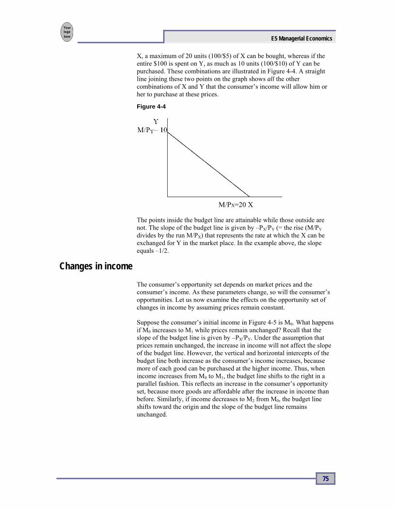
X, a maximum of 20 units (100/$5) of X can be bought, whereas if the entire $100 is spent on Y, as much as 10 units (100/$10) of Y can be purchased. These combinations are illustrated in Figure 4-4. A straight line joining these two points on the graph shows all the other combinations of X and Y that the consumer’s income will allow him or her to purchase at these prices.

Figure 4-4

M/PX=20 X

The points inside the budget line are attainable while those outside are not. The slope of the budget line is given by –PX/PY (= the rise (M/PY divides by the run M/PX) that represents the rate at which the X can be exchanged for Y in the market place. In the example above, the slope equals –1/2.

Changes in income

The consumer’s opportunity set depends on market prices and the consumer’s income. As these parameters change, so will the consumer’s opportunities. Let us now examine the effects on the opportunity set of changes in income by assuming prices remain constant.

Suppose the consumer’s initial income in Figure 4-5 is M0. What happens if M0 increases to M1 while prices remain unchanged? Recall that the slope of the budget line is given by –PX/PY. Under the assumption that prices remain unchanged, the increase in income will not affect the slope of the budget line. However, the vertical and horizontal intercepts of the budget line both increase as the consumer’s income increases, because more of each good can be purchased at the higher income. Thus, when income increases from M0 to M1, the budget line shifts to the right in a parallel fashion. This reflects an increase in the consumer’s opportunity set, because more goods are affordable after the increase in income than before. Similarly, if income decreases to M2 from M0, the budget line shifts toward the origin and the slope of the budget line remains unchanged.

Module 4

76

Figure 4-5

M2/PX M0/PX M1/PX X

Changes in price

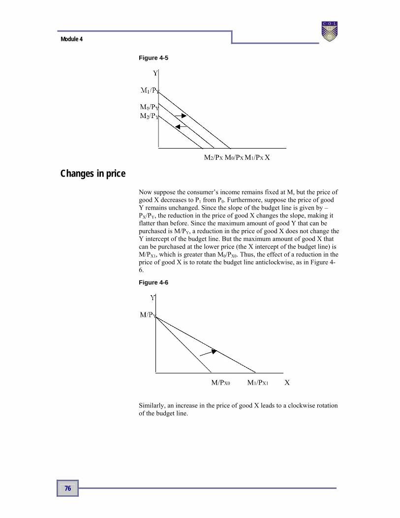
Now suppose the consumer’s income remains fixed at M, but the price of good X decreases to P1 from P0. Furthermore, suppose the price of good Y remains unchanged. Since the slope of the budget line is given by –PX/PY, the reduction in the price of good X changes the slope, making it flatter than before. Since the maximum amount of good Y that can be purchased is M/PY, a reduction in the price of good X does not change the Y intercept of the budget line. But the maximum amount of good X that can be purchased at the lower price (the X intercept of the budget line) is M/PX1, which is greater than M0/PX0. Thus, the effect of a reduction in the price of good X is to rotate the budget line anticlockwise, as in Figure 4-6.

Figure 4-6

M/PX0 M1/PX1 X

Similarly, an increase in the price of good X leads to a clockwise rotation of the budget line.

E5 Managerial Economics

77

Consumer equilibrium

The principal assumption upon which the theory of consumer behaviour rests is that consumers attempt to allocate their limited money incomes to purchase available goods and services so as to maximise their satisfaction (utility). In other words, consumers’ indifference map provides a diagrammatic representation of a consumer’s taste and intensity of desire for different product combinations while the consumer’s purchasing power (and thus ability to satisfy material wants) is reflected by the line of attainable combinations. Putting the two together shows all the desired product combinations on the indifference curves that are also attainable.

As illustrated in Figure 4-7, the point of equilibrium can be located by drawing the budget line on the indifference map for goods X and Y. Since the number of indifference curves upon the indifference map is infinite, one curve will be tangent to the budget line regardless of where the budget line lies. The point of tangency is the point of equilibrium, representing the attainable combination of X and Y that gives the highest level of utility. As indicated in this Figure, the budget line is tangent to the indifference curve, I2, at point E, where the consumer acquires YE units of Y and XE of X. Since indifference curves may not intersect, it is clear that I2 represents the highest level of utility that can be obtained with the budget available. An indifference curve representing a higher level, I3, does not touch the budget line, and hence is unattainable, whereas an indifference curve representing a lower level, I1, intersecting the budget line at two places is inferior to I2. It should not be difficult to see why point E is preferable to any other point on the budget line. For example, point B also exhausts the income, but it clearly offers less utility than point E because it lies on a lower indifference curve.

Figure 4-7

XE X

Note, at the point of tangency between the indifference curve and the budget line, the slope of the indifference curve equals the slope of the budget line, that is,

y

x

P

PMRS

(5)

Module 4

78

The condition for maximising satisfaction requires that the consumer allocate his or her purchasing power so that the marginal rate of substitution of X for Y is equal to the ratio of the price of X to the price of Y. The interpretation of this condition is straightforward. The MRS defines the rate at which the consumer is willing to exchange X for Y. The price ratio (PX/PY) shows the rate at which the consumer can exchange X for Y. Unless the two rates are equivalent, it is possible for the consumer to alter purchases of X and Y and achieve a greater degree of satisfaction.

Suppose that at the current purchase combination, MRS = 4, meaning that the consumer is willing to exchange four units of Y for one more unit of X. If PX = $6 and PY = $2, then the consumer need only give up three units of Y at $2 each to obtain the dollars needed to buy another unit of X. This situation is reflected by point B in Figure 4-7, where the slope of the indifference curve is steeper than the slope of the budget line. This means the consumer is willing to give up more of good Y to get an additional unit of good X than he or she actually has to give up, based on the market. Confronted with these circumstances, it is in the consumer’s interest to consume less of good Y and more of good X. This substitution continues until ultimately the consumer is at point E, in Figure 4-7, where the MRS is equal to the ratio of prices.

In general, then, consumer maximization of satisfaction requires equality between the marginal rate of substitution for any pair of products and the ratio of their prices, otherwise some exchange can be made which will increase consumers’ overall satisfaction.

Demonstration problem

Suppose an individual uses exactly two pats of butter on each piece of toast. If toast costs $0.20/slice and butter costs $0.10/pat, find this individual’s best affordable bundle if she has $12 per month to spend on toast and butter.

Answer:

The individual is willing to exchange one piece of toast for two pats of butter, i.e., MRS = 2. At the same time, the price ratio (Ptoast/Pbutter) = 2. Therefore the individual is already maximising her satisfaction since MRS = (Ptoast/Pbutter). Therefore her $12 budget should be allocated in such a way that for every piece of toast that she consumes she will consume two pats of butter – 60 pats of butter and 30 toasts.

E5 Managerial Economics

79

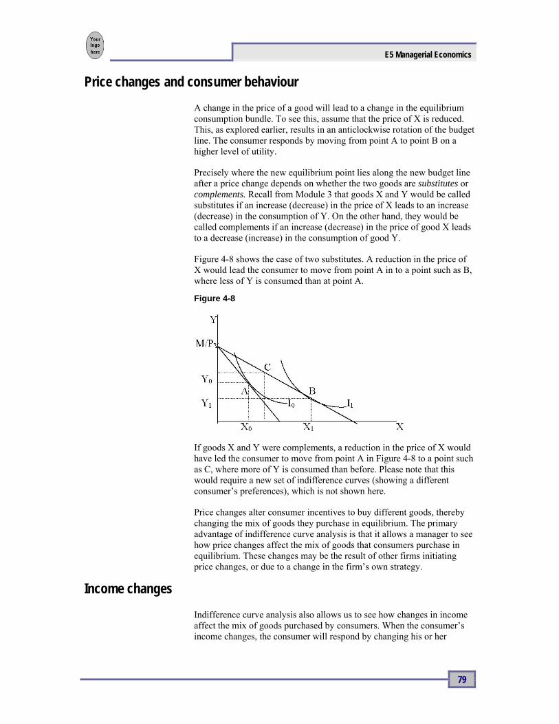
Price changes and consumer behaviour

A change in the price of a good will lead to a change in the equilibrium consumption bundle. To see this, assume that the price of X is reduced. This, as explored earlier, results in an anticlockwise rotation of the budget line. The consumer responds by moving from point A to point B on a higher level of utility.

Precisely where the new equilibrium point lies along the new budget line after a price change depends on whether the two goods are substitutes or complements. Recall from Module 3 that goods X and Y would be called substitutes if an increase (decrease) in the price of X leads to an increase (decrease) in the consumption of Y. On the other hand, they would be called complements if an increase (decrease) in the price of good X leads to a decrease (increase) in the consumption of good Y.

Figure 4-8 shows the case of two substitutes. A reduction in the price of X would lead the consumer to move from point A in to a point such as B, where less of Y is consumed than at point A.

Figure 4-8

If goods X and Y were complements, a reduction in the price of X would have led the consumer to move from point A in Figure 4-8 to a point such as C, where more of Y is consumed than before. Please note that this would require a new set of indifference curves (showing a different consumer’s preferences), which is not shown here.

Price changes alter consumer incentives to buy different goods, thereby changing the mix of goods they purchase in equilibrium. The primary advantage of indifference curve analysis is that it allows a manager to see how price changes affect the mix of goods that consumers purchase in equilibrium. These changes may be the result of other firms initiating price changes, or due to a change in the firm’s own strategy.

Income changes

Indifference curve analysis also allows us to see how changes in income affect the mix of goods purchased by consumers. When the consumer’s income changes, the consumer will respond by changing his or her

Module 4

80

optimal bundle of goods (X and Y). Normally, increases in income, all else remaining constant, will lead to increased demand for the products available to the consumer. We show such a situation in Figure 4-9, where the consumer’s income has increased and that consumer subsequently purchases more of both products available. Note that at the initial prices and income level (M0), and given the consumer’s taste and preference pattern (indicated by the indifference curves), the consumer maximises at point A.

Now suppose the consumer’s income increases to M1 so that his or her budget line shifts out in a parallel fashion. Clearly the consumer can now achieve a higher level of satisfaction than before. This particular consumer finds it in his or her interest to choose bundle B in Figure 4-9, where the indifference curve through point B is tangent to the new budget line.

Figure 4-9

In this case, the quantity demanded of both products has increased as a result of the increase in the consumer’s income. Since income and quantity demanded moved in the same direction, we say that the income effect was positive for both goods. We call such products normal goods.

For some products the income effect is negative, meaning that if income increases, the quantity demanded of those products actually declines. This may happen to a product that is an inferior substitute for some superior product. As people become richer, they tend to switch away from inferior goods to superior substitutes. Conversely, as incomes fall (in a recession, for example), people tend to switch back to the inferior substitutes as they find themselves unable to afford the superior substitutes.

In Figure 4-10 we show the income effect for an inferior good. The product on the horizontal axis, travel by train, is an inferior good, and travel by air is a superior substitute for this particular consumer. Note that when the consumer’s income increases and the budget line moves outward, the quantity demanded of travel by train actually decreases while travel by air increases. This consumer, now able to afford more air travel, substitutes away from the inferior good and in favour of the

E5 Managerial Economics

81

superior good. Looking at this from the opposite perspective, if the consumer’s income were to fall from the higher level to the lower level, the consumer would reduce consumption of the superior good and increase consumption of the inferior good.

Figure 4-10

For any particular product at any particular point in time, some consumers may regard that product as a superior good while others may regard it as an inferior good. This difference in attitude toward a particular product stems from a difference in income levels and/or a different pattern of tastes and preferences.

The income and substitution effects of a price change

We can combine our analysis of price and income changes to gain a better understanding of the effect of a price change on consumer behaviour. The effect of the price change can be thought of as comprising two separate effects, known as the income effect and the substitution effect. When a product’s price falls (and all other things remain unchanged), the consumer experiences an increase in his or her real income. Real income is the purchasing power of money income. When the price of a particular good falls, the consumer can buy the same combination as before and have some money left over. This additional real income can then be spent, both on the product whose price has fallen and on other products. Normally, the income effect of a price reduction causes the consumer to buy a little more of the product in question, but if the product in question is an inferior substitute for some other product, the consumer may reduce purchases of the inferior product (whose price fell) in favour of the other product.

The second part of the price effect is the substitution effect. When the price of a product falls, consumers will tend to substitute in favour of that product because it is now cheaper relative to other substitute products that serve the same need. Thus, when the price of a product falls, all else being kept constant, the consumer would normally buy more of that product, first because his or her real income has increased, and second

Module 4

82

because he or she substitutes toward that product and away from other substitutes that are now relatively more expensive.

Suppose a consumer initially is in equilibrium at point A in Figure 4-11, along the budget line connecting points J and K. Suppose the price of good X decreases so that the budget line rotates anti-clockwise, and becomes the budget line connecting points J and L. The consumer now maximises his or her satisfaction at point C. The movement from A to C is referred to as the total effect. The total effect, however, is composed of substitution and income effects. The substitution effect reflects a movement along an indifference curve, from A to B, thus isolating the effect of a relative price change on consumption: XB – XA. The income effect results from a parallel shift in the budget line; thus it isolates the effect of increases of ‘real income’ on consumption and is represented by the movement from B to C: XC – XB. The total effect of a price decrease, which is what we observe in the marketplace, is the movement from A to C: XC – XA. Therefore, the total effect of a change in consumer behaviour results not only from the effect of a lower relative price of good X (the movement from A to B) but also from the increased real income of the consumer (the movement from B to C).

Figure 4-11

Demonstration problem

Suppose your product is a cyclical product, that is, sales vary directly with the economy. How can this information be useful to you when considering alternative products to include in your store?

Answer:

If you expand your offerings to include more normal goods, you will continue to have an operation that sells more during an economic boom than during a recession. However, if you include in your operation some inferior goods, the demand for these products will increase during bad economic times for normal goods. This is not to say that the optimal mix of products

E5 Managerial Economics

83

involves a 50-50 mix of normal and inferior goods; indeed, the optimal mix will depend on your own risk preference. Therefore, you may be better off diversifying, at least to a degree.

Demonstration problem

Does running a gourmet food store involve a higher level of risk of going out of business than running a supermarket, or vice versa, when the economy heads for a recession?

Answer:

Note that gourmet shops sell almost exclusively normal goods, while supermarkets have a more ‘balanced portfolio’ of normal and inferior goods. This explains why, during recessions, many gourmet shops go out of business while supermarkets do not. This is the case because the outlet that sells low, or even perhaps negative, income elastic products tends to survive and in fact do well in a recession.

Corner solutions

In all the examples considered so far, the optimal consumer basket has been interior, meaning that the consumer consumes positive amounts of both goods. In reality, though, a given consumer will not purchase positive amounts of all available goods. For example, not all consumers own a car or a house. Some consumers may not spend money on tobacco or alcohol. If the consumer cannot find any interior basket at which the budget line will be tangent to an indifference curve, then he or she may find an optimal basket at a corner point, that is, at a basket along an axis, where one of the goods is not purchased at all. If an optimum occurs at a corner point, the budget line may not be tangent to an indifference curve at the optimal basket.

Let’s consider again our consumer who chooses between just two goods, food and clothing. If the consumer’s indifference map is as illustrated in Figure 4-12, no indifference curve is tangent to his or her budget line. At any interior basket on the budget line, such as basket B, the slope of the indifference curve is steeper (more negative) than the slope of the budget line. This means that MRS > PX/PY. In this case, our consumer is willing to exchange more Y for an additional unit of X than he or she has to, based on the market. This is true not only at basket B, but at all baskets on the budget line. The consumer would continue to substitute X for Y, moving along the budget line until he or she reaches the corner point basket C. At basket C the slope of the indifference curve I2 is still steeper than the slope of the budget line; he or she would like to substitute more X for Y if that were possible. But no further substitution is possible because no more X can be purchased beyond basket C. Therefore the optimal choice for this consumer is basket C, because that basket gives the consumer the highest utility possible on the budget line.

Module 4

84

Figure 4-12

CX

Application of indifference curves

Quantity discounts

In many instances sellers offer consumers quantity discounts. We can use indifference curve analysis to understand how such discounts work. Here is an example. Suppose a video/DVD store sells its products according to the following formula. For the purchase of the first eight videos/DVDs the seller charges a price of $15 for each video/DVD. However, a hefty discount is offered on purchase of each additional unit, $10 per video/DVD. Figure 4-13 shows how the quantity discounts affect the consumer’s behaviour assuming that the buyer starts with a fixed budget of $300 to be spent on all goods including video/DVD.

Figure 4-13

As shown in Figure 4-13, in the absence of a quantity discount, each unit sells for $15 and the budget line facing the consumer is represented by JK. The slope of this line is (–15). Point J, the vertical intercept is a point where the buyer buys no video/DVD, and keeps his or her money for other products. The vertical axis can hence be regarded as a composite good (all other goods). Point K, on the other hand, is a point where all $300 is spent on video/DVD. The consumer, however, would choose

E5 Managerial Economics

85

point A, where eight video/DVDs are purchased. Suppose the discount kicks in. The budget line is now represented by the line JAL, a broken line. The upper segment of the budget line (JA) has the slope of (15), whereas the bottom segment (AL) has the slope of (–10), and the consumer will buy the total of 12 videos/DVDs, point B. The quantity discount scheme has induced the consumer to purchase an additional four units.

Voucher versus cash subsidies

Governments in most countries often employ a wide range of publicly subsidised ‘assisted housing’ programmes. One of the main objectives of all of these programmes is to provide access to a primary human requirement for those most in need. For instance in Canada, the current annual cost of housing subsidies is estimated at more than $5 billion. Increasingly, in the allocation of the limited stock of subsidised housing units, the focus is on those high-need, low-income families who have to spend more than 30 per cent of their family income to rent adequate accommodation.

Suppose the consumer (household’s) preferences for housing and other goods are represented by the indifference curves as in Figure 4-14. Let the Y-axis denote the composite good (measured in dollars per month) and X represents the housing units. Assume that this household has a monthly budget of $M and must pay PX for each unit it rents. The budget line is represented by JK. Given the budget line and the indifference curves, equilibrium is found at point A with XA units of housing. The consumer spends ($M – YA) on housing and the rest, YA, on other goods.

Now suppose the government steps in to increase the housing consumption. There are two types of programmes that might be implemented to increase the consumer’s purchases of housing: (a) the subsidy as an additional amount of housing the family receives, coupon (housing voucher) or (b) the subsidy as an additional income, cash subsidy.

Figure 4-14

Module 4

86

If the consumer receives a cash subsidy of $S from the government, the budget line shifts from JK to LN. If the government gives the consumer a voucher also worth $S that can only be spent on housing, the budget line will be represented by JHN. Because the consumer cannot apply the voucher to purchase other goods, the maximum he or she can spend on other goods is still $M, whereas in the case of a cash (income) subsidy, the consumer is free to allocate whatever amount he or she wishes to allocate to housing and other goods. Assuming that the consumer’s preferences are represented by the set of indifference curves I1 and I2, he or she will be indifferent between a cash subsidy and a voucher, and the choice of the programme does not matter. The consumer’s choice will be point B in either case.

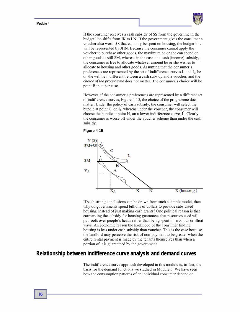
However, if the consumer’s preferences are represented by a different set of indifference curves, Figure 4-15, the choice of the programme does matter. Under the policy of cash subsidy, the consumer will select the bundle at point C, on I4, whereas under the voucher, the consumer will choose the bundle at point H, on a lower indifference curve, I3. Clearly, the consumer is worse off under the voucher scheme than under the cash subsidy.

Figure 4-15

If such strong conclusions can be drawn from such a simple model, then why do governments spend billions of dollars to provide subsidised housing, instead of just making cash grants? One political reason is that earmarking the subsidy for housing guarantees that resources used will put roofs over people’s heads rather than being spent in frivolous or illicit ways. An economic reason the likelihood of the consumer finding housing is less under cash subsidy than voucher. This is the case because the landlord may perceive the risk of non-payment to be greater when the entire rental payment is made by the tenants themselves than when a portion of it is guaranteed by the government.

Relationship between indifference curve analysis and demand curves

The indifference curve approach developed in this module is, in fact, the basis for the demand functions we studied in Module 3. We have seen how the consumption patterns of an individual consumer depend on

E5 Managerial Economics

87

variables that include the prices of substitute goods, the prices of complementary goods, tastes (the shape of indifference curves), and income. We conclude by examining the link between indifference curve analysis and demand curves.

Individual demand

Recall from Module 3 that a market demand curve is a relationship that tells how much of a good the market as a whole wants to purchase at various prices. Suppose we want to generate a demand schedule for a good, X, not for the market as a whole but for only a single consumer. Holding income, preferences, and the prices of all other goods constant, how will a change in the price of shelter affect the amount X the consumer buys? To answer this question, we begin with this consumer’s indifference map, with X on the horizontal axis and the composite good Y on the vertical axis, Figure 4-16(a). The consumer initially is in equilibrium at point A, where income is fixed at M, and prices are PXA and PYA. But when the price of good X falls to the lower level, indicated by PXB (PXB < PXA ), the consumer reaches a new equilibrium at point B. The important thing to notice is that the only change that caused the consumer to move from A to B was a change in the price of good X; income and the price of good Y are held constant in the diagram. When the price of good X is PXA the consumer consumes XA units of good X; when the price falls to PXB, the consumption of X increases to XB.

The panel (b) in Figure 4-16 shows this relationship between the price of good X and the quantity consumed of good X. This consumer’s demand curve for good X indicates that, holding other things constant, when the price of good X is PXA the consumer will purchase XA units of X; when the price of good X is PXB, the consumer will purchase XB units of X.

Module 4

88

Figure 4-16

The line connecting point A to point B in panel (b) represents the demand curve for our consumer. An individual consumer’s demand curve is like the market demand curve in that it tells the quantities the consumer will buy at various prices.

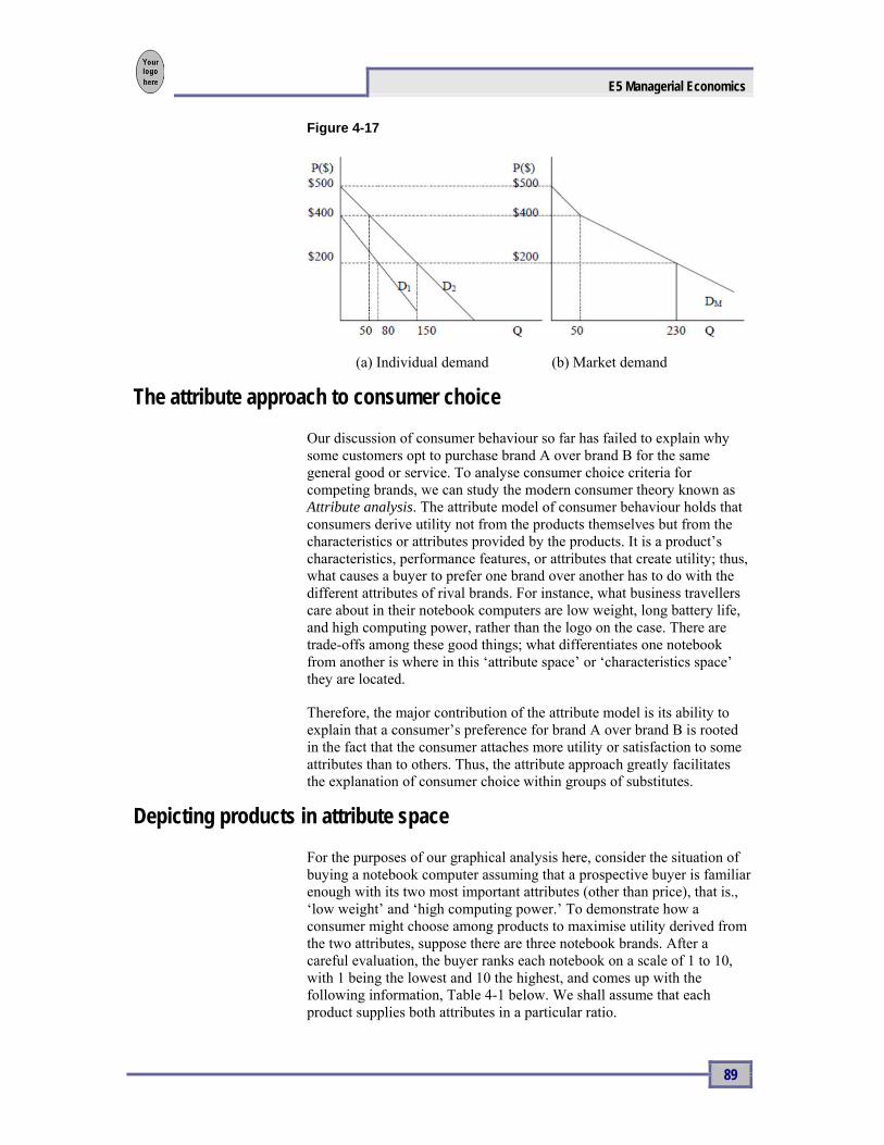
Market demand

The market demand curve is the horizontal summation of individual demand curves and indicates the total quantity all consumers in the market would purchase at each possible price. This concept is illustrated graphically in Figures 4-17(a) and 4-17(b). The curves D1 and D2 represent the individual demand curves of two hypothetical consumers: Individual 1 and Individual 2. When the price is $500, Individual 1 and Individual 2 buy 0 units. Thus, at the market level, 0 units are sold when the price is $500, and this is one point on the market demand curve (labeled DM in Figure 4-17(b)). When the price is $400, Individual 1 buys 50 units (point A) and Individual 2 buys 0 units (point B). Thus, at the market level 50 units are sold when the price is $400, and this is another point (point A + B) on the market demand curve. When the price of good is $200, Individual 1 buys 150 units and Individual 2 buys 80 units; thus, at the market level, 230 units are sold when the price is $200.

E5 Managerial Economics

89

Figure 4-17

(a) Individual demand (b) Market demand

The attribute approach to consumer choice

Our discussion of consumer behaviour so far has failed to explain why some customers opt to purchase brand A over brand B for the same general good or service. To analyse consumer choice criteria for competing brands, we can study the modern consumer theory known as Attribute analysis. The attribute model of consumer behaviour holds that consumers derive utility not from the products themselves but from the characteristics or attributes provided by the products. It is a product’s characteristics, performance features, or attributes that create utility; thus, what causes a buyer to prefer one brand over another has to do with the different attributes of rival brands. For instance, what business travellers care about in their notebook computers are low weight, long battery life, and high computing power, rather than the logo on the case. There are trade-offs among these good things; what differentiates one notebook from another is where in this ‘attribute space’ or ‘characteristics space’ they are located.

Therefore, the major contribution of the attribute model is its ability to explain that a consumer’s preference for brand A over brand B is rooted in the fact that the consumer attaches more utility or satisfaction to some attributes than to others. Thus, the attribute approach greatly facilitates the explanation of consumer choice within groups of substitutes.

Depicting products in attribute space

For the purposes of our graphical analysis here, consider the situation of buying a notebook computer assuming that a prospective buyer is familiar enough with its two most important attributes (other than price), that is., ‘low weight’ and ‘high computing power.’ To demonstrate how a consumer might choose among products to maximise utility derived from the two attributes, suppose there are three notebook brands. After a careful evaluation, the buyer ranks each notebook on a scale of 1 to 10, with 1 being the lowest and 10 the highest, and comes up with the following information, Table 4-1 below. We shall assume that each product supplies both attributes in a particular ratio.

Module 4

90

Table 4-1: Attributes and Prices of Three Brands of Notebook Computers

Attribute Rating

Notebook Brand

Notebook Price

Low Weight

High Computing

Power

Ratio of Low Weight

to High

Computing Power

A $2,500 9 4 2.25

B 2,800 7 6 1.16

C 3,200 5 9 0.55

In Figure 4-18, below, each notebook brand is shown in the attribute space as a ray drawn from the origin. Graphically, the slope of each ray is determined by the ratio of low weight to computing power, as listed in the last column in the table. If the buyer buys notebook A, he or she will travel out along the steepest ray, absorbing the two attributes in the ratio 2.25. The other notebook computers are indicated by the lower rays because these offer the two attributes at lower ratios. If the traveller buys notebook B, he or she will travel along the second steepest ray with the slope of 1.16. Finally, for brand C, the ratio is 0.55.

What determines how far along each ray the buyer could go and how much of each product the buyer can purchase depends on the buyer’s budget (budget constraint). In the case of an indivisible purchase, such as purchase of a car or a notebook computer – the products that are, on the one hand, available only in discrete units and, on the other hand, the price of which are large in relation to the consumer’s income – the consumer is expected to stop at purchasing just one unit of the product: one car and one notebook computer. This, of course, implicitly assumes the buyer’s budget is large enough to permit the purchase of all three brands despite the price differences.

Following this logic, the efficiency frontier, which is the outer boundary of the attainable combinations of attributes, is obtained. It is called ‘efficient’ because only combinations on this frontier allow the consumer to maximise utility. This frontier consists of the points joining the limit points – points A, B, and C – on each product ray. Each point is found by first dividing the buyer’s income by the price of the respective product in order to determine the number of the units of the product, and then multiplying the outcome by the attribute content of each unit. The point depicted along each ray shows the maximum intake of the two attributes that can be obtained by consuming each notebook.

Utility maximisation from attributes

Just as consumers can express preference or indifference between combinations of products, they can express preference of indifference

E5 Managerial Economics

91

between combinations of attributes. At any particular combination of ‘light weight’ and ‘high computing power’, our buyer will be able to express a marginal rate of substitution between the two attributes: at any point, an extra unit of ‘low weight’ will be worth giving up some amount of ‘high computing power.’ These evaluations produce a set of indifference curves expressing the buyer’s tastes and preferences at each possible attribute combination. Since our buyer cannot mix brands but rather needs to choose one notebook brand or another, he or she must be content with the constrained point: A, B, or C, Figure 4-18. Therefore, the efficient frontier is represented by the kinked line ABC. The buyer maximises utility by choosing the notebook brand with the attribute combination on the highest indifference curve attainable, I*.

Of these options, point B allows the buyer to attain the highest indifference curve, I*.

Figure 4-18

Module 4

92

Module summary

Summary

The utility approach to consumer behaviour is grounded upon psychological principles, and is best explained in terms of utility. Conceptually, utility can be measured in cardinal units, as in Module 2, or ordinal approach, as discussed in this module, in which case the consumer is able to rank products in order of preference. Consumer equilibrium is reached when the marginal utility per dollar is the same for all products, or when the slope of the indifference curve and the slope of the budget line are the same. The consumer’s demand curve for a particular product is directly related to the marginal utility of that product. The downward sloping demand curve is due to the law of diminishing marginal utility. In general, the individual’s demand curve consists of two effects, the substitution effect and the income effect. The income effect may be positive or negative depending on the taste and preferences of the consumer. Changes in the consumer’s income will change the quantity demanded at a given price level. The quantity demanded of normal goods will move in the same direction as income, whereas the quantity demanded of inferior goods will move in the opposite direction to income.

The attribute approach to consumer behaviour gives several valuable insights into consumer choice, which are not readily apparent using the product approach. This approach allows the entire range of substitutes available to the consumer to be depicted on the same graph. It is, therefore, able to explain why a consumer buys one brand of a product over another one. Furthermore, this approach can explain why a consumer will purchase combinations of substitute products.

E5 Managerial Economics

93

Assignment

Assignment

1. A consumer has an income of $50. He can choose any combination of product X and product Y for consumption. If price of X (Px) is $5 and price of Y (Py) is $2.50, draw the budget line of the consumer. Find the market rate of substitution. What is the maximum quantity of Y that he can purchase? If the income goes up to $75, then how will the budget line change? Find the maximum quantity of Y that he can purchase with the new budget.

2. A consumer can choose any combination of apples and oranges. A, B, and C are three different points on his indifference curve. If he moves from A to B he gives up two oranges for one apple. If he moves from B to C then he gives up one orange for one apple. Do the consumer’s preferences comply with the diminishing marginal rate of substitution? Explain.

Module 4

94

Assessment

Assessment

1. Consider the problem in question 2. If the price of apples is $0.50 per unit and the price of oranges is $0.25 per unit, then with an income of $10 at which point (among points A, B, and C) will he maximise his welfare? Explain. If welfare is not maximised at any of these points, then explain how he should change his consumption.

2. Prices of food and clothing are currently $10 per unit and $25 per unit respectively. With an income of $500, find the market rate of substitution. Suppose that the consumer’s preference shows that marginal rate of substitution at some point is two units of food for one unit of clothing. Given that the consumer’s indifference curve shows a diminishing marginal rate of substitution, how should the consumer adjust his consumption to maximise utility given the budget constraint?

E5 Managerial Economics

95

Assessment answers 1. Market rate of substitution = 0.5/0.25 = 2, MRS at A = 2

At A the consumer maximises welfare.

2. Market rate of substitution = 25/10 = 2.5

MRS = 2

The consumer can improve welfare by increasing consumption of food and reducing consumption of clothing. Given that her preferences show diminishing MRS, with this change she can reach a point where her preference will be to give up 2.5 units of food for 1 unit of clothing, at which point MRS will be equal to the price ratio, maximising her utility.

Module 4

96

References

References

Baumol, W. J. (1967). Business Behavior, Value and Growth, Rev. Ed. New York: Harcourt Brace Johanovich.

Besanko, D., & Braeutigam, R. (2002). Microeconomics: An Integrated Approach. New York: Wiley & Sons.

Douglas, J. E. (1992). Managerial Economics: Analysis and Strategy. Upper Saddle River, NJ: Prentice Hall.

Lancaster, K. (1971). Consumer Demand: A New Approach. New York: Columbia University.

Pindyck, R. S., & Rubinfeld, D. (2001). Microeconomics, 5th Edition. Upper Saddle River, NJ: Prentice Hall.