The Term Structure of Implied Forward Volatility: … · The Term Structure of Implied Forward...
26
The Term Structure of Implied Forward Volatility: Recovery and Informational Content in the Corn Options Market by Thorsten M. Egelkraut, Philip Garcia, and Bruce J. Sherrick Suggested citation format: Egelkraut, T. M., P. Garcia and B. J. Sherrick. 2003. “The Term Structure of Implied Forward Volatility: Recovery and Informational Content in the Corn Options Market.” Proceedings of the NCR-134 Conference on Applied Commodity Price Analysis, Forecasting, and Market Risk Management. St. Louis, MO. [http://www.farmdoc.uiuc.edu/nccc134].
-
Upload
nguyendung -
Category
Documents
-
view
238 -
download
1
Transcript of The Term Structure of Implied Forward Volatility: … · The Term Structure of Implied Forward...
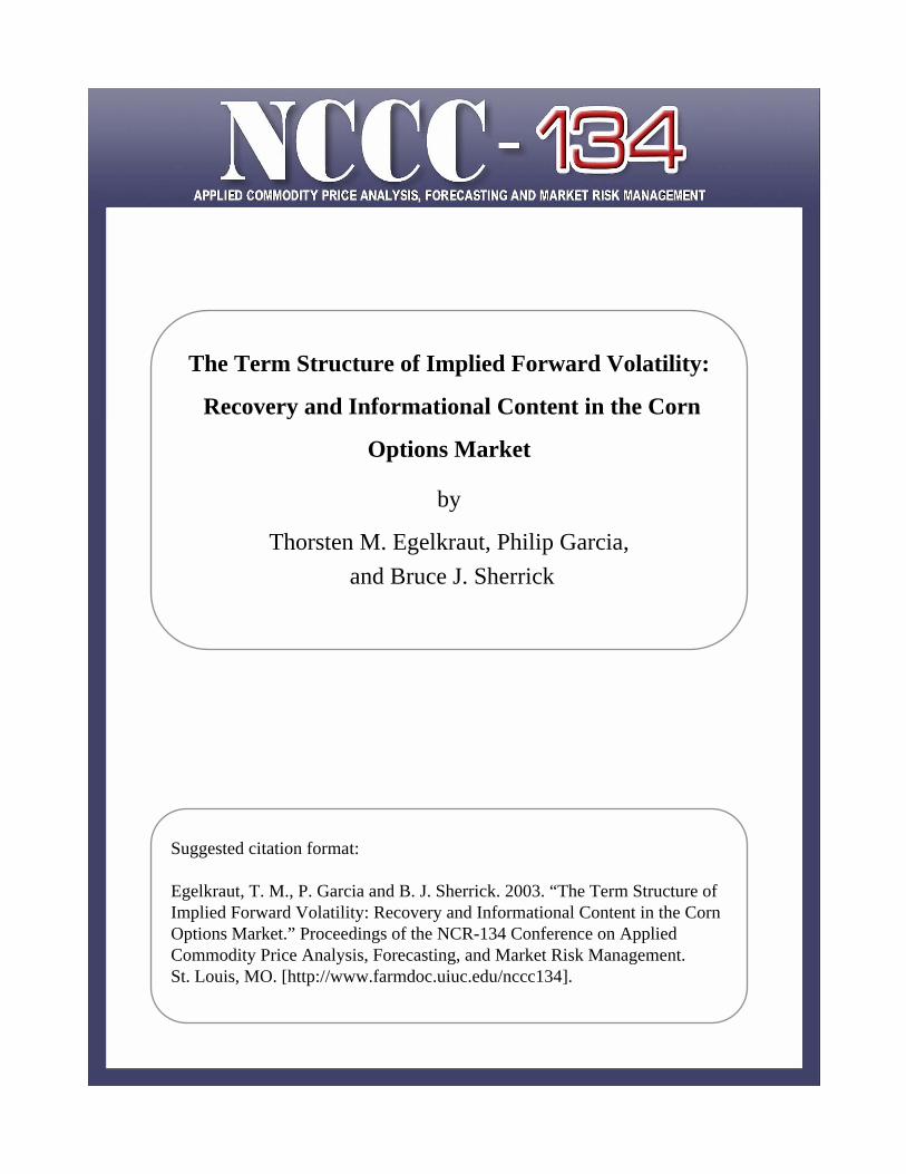
The Term Structure of Implied Forward Volatility:
Recovery and Informational Content in the Corn
Options Market
by
Thorsten M. Egelkraut, Philip Garcia,and Bruce J. Sherrick
Suggested citation format:
Egelkraut, T. M., P. Garcia and B. J. Sherrick. 2003. “The Term Structure of Implied Forward Volatility: Recovery and Informational Content in the Corn Options Market.” Proceedings of the NCR-134 Conference on Applied Commodity Price Analysis, Forecasting, and Market Risk Management. St. Louis, MO. [http://www.farmdoc.uiuc.edu/nccc134].
The Term Structure of Implied Forward Volatility: Recovery and Informational Content in the Corn Options Market
Thorsten M. Egelkraut
Philip Garcia
Bruce J. Sherrick*
Paper presented at the NCR-134 Conference on Applied Commodity Price Analysis, Forecasting, and Market Risk Management
St. Louis, Missouri, April 21-22, 2003
Copyright 2003 by Thorsten M. Egelkraut, Philip Garcia, and Bruce J. Sherrick. All rights reserved. Readers may make verbatim copies of this document for non-commercial
purposes by any means, provided that this copyright notice appears on all such copies.
*Thorsten M. Egelkraut, Philip Garcia, and Bruce J. Sherrick are Graduate Fellow ([email protected]), Professor and T. A. Hieronymus Chair, and Associate Professor in the Department of Agricultural and Consumer Economics, University of Illinois at Urbana-Champaign. The authors are also in the Office of Futures and Options Research.
1
The Term Structure of Implied Forward Volatility: Recovery and Informational Content in the Corn Options Market
Options with different maturities can be used to generate volatility estimates for non-overlapping future time intervals. This paper develops the term structure of volatility implied by corn futures options, and evaluates the informational content of the implied forward volatility as a predictor of subsequent realized volatility. Using data from 1987-2001 and employing a flexible method to obtain the implied forward volatilities, two types of information are examined: 1) the market’s estimate of future realized volatility for the nearby interval of the term structure and, 2) the market’s expectation of the direction and magnitude of change of future realized volatility over time. In contrast to previous research, the results indicate that the implied forward volatilities anticipate the realized volatilities reasonably well. For the nearby interval of the term structure, the implied forward volatilities provide unbiased forecasts and capture a larger portion of the systematic variability in the realized volatilities than forecasts based on historical volatilities. Using information on the direction and magnitude of change in volatility over time, we find that the early-year options forecast volatility about as well as the three-year moving average and better than the naïve forecast, while later-year options and alternative forecasts are less able to predict the direction and magnitude of changing volatility. During this later-year period, the implied forward volatilities tend to over-predict the magnitude of actual volatility. Overall, we find that the term structure of volatility implied by corn futures options contains information on future realized volatility. Keywords: corn options, implied forward volatility, informational content, term structure Introduction Price risk, generally expressed as volatility, has been shown to affect input and output decisions in a variety of economic situations. In a decision-making context, information about future volatility is particularly important to market participants as it permits them to assess alternative allocations of resources in a more relevant framework. In futures markets for example, information about future volatility can provide market participants with an understanding of the relative costs and risks of placing and offsetting hedges during different time periods. Increased volatility can correspond to more frequent margin calls, shortening the time that investors have to respond with new funds, and thereby putting a greater portion of investors’ wealth at risk. Information about future volatility can also provide insight into whether holding a particular commodity, e.g., storing harvested grain, will be consistent with individual risk preferences.1 The needed estimates of future volatility over a particular time period can be obtained from observed options premiums by inverting a theoretical pricing model. However, as the volatility implied in options premiums is only an expected average, market participants still face the risk of not knowing when volatility will be below or above this average. Although not often realized, this important information is also contained in options prices.
Market participants and researchers have largely overlooked the possibility of
decomposing the expected average volatilities implied in options with different maturities into 1 Information about the future volatility in prices might also be used in risk-response econometric analysis.
2
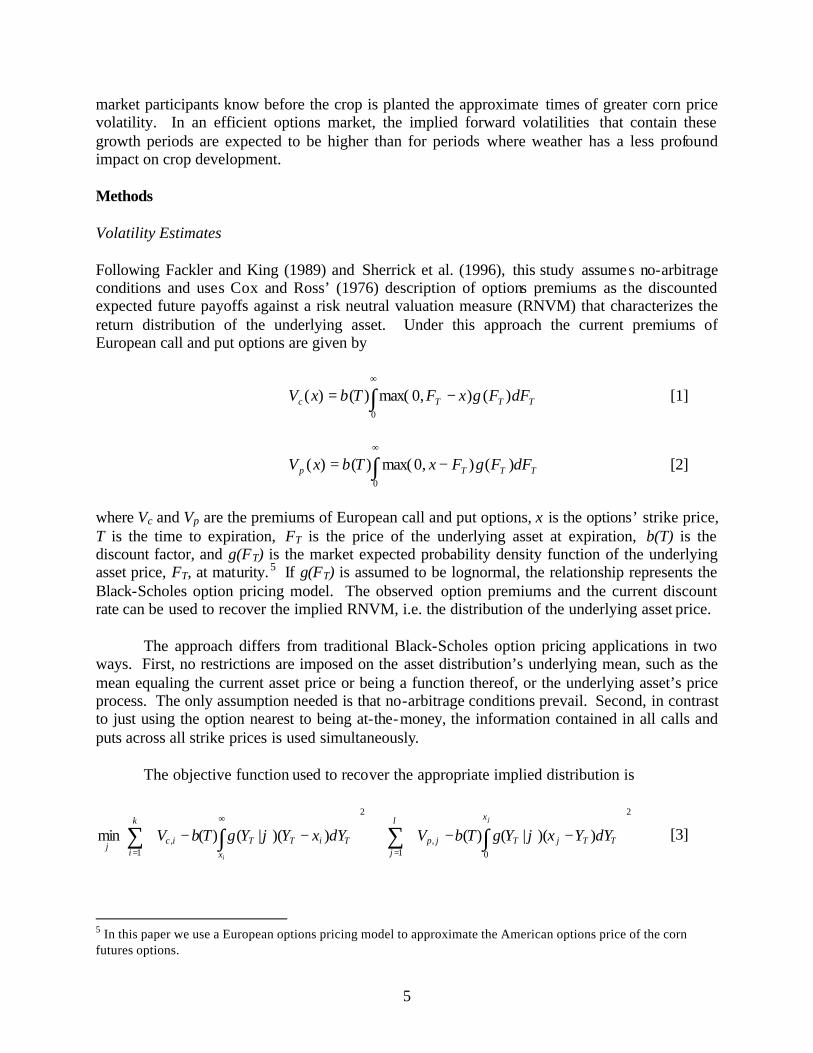
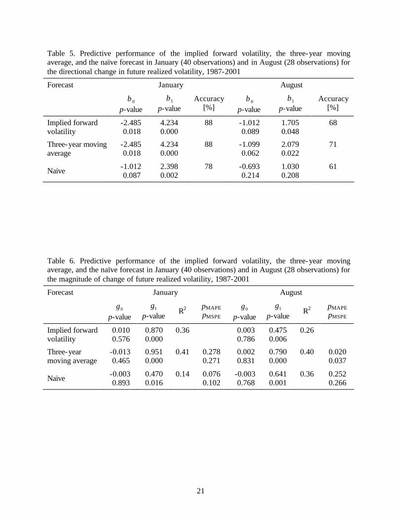
implied forward volatilities. These forward volatilities, also known as forward-forward volatilities, refer to the expected average volatilities between the expiration dates of two options with successive maturities. Figure 1 illustrates this idea for a pair of options. At 0=t , the options expiring at α−= eTt and eTt = , 0>α , imply two different average volatilities,
ασ
−− eTiv 0,
and eTiv −0,σ . These expected average volatilities, however, are not the only information about
future volatility that can be recovered from the options prices. The options prices also hold information about the implied forward volatility,
ee TTifv −−ασ , , over the interval from α−eT to eT .
Using options with several different expirations, market participants can infer an implied forward volatility curve - the term structure of volatility. 2 Hence, the implied volatilities recovered from options prices contain information about the expected average volatilities until expiration, and also the expected average volatilities during non-overlapping time intervals.
This paper identifies a procedure to generate the term structure of volatility implied by
options prices, and evaluates the informational content of futures options on a storable agricultural commodity. Specifically, we investigate the term structure and the ability of the implied forward volatility to predict realized volatility of corn futures prices. As a determinant crop, corn is characterized by a few short, but critical, time periods in its growing cycle during which environmental factors such as weather have a greater impact on yields and price variability than during other periods. Because these critical periods repeat annually, the associated greater volatility provides a natural test of the implied forward volatilities’ forecast ability. In the analysis, we employ a recently advanced method to obtain the implied volatilities which recovers all information about future volatility available from the options prices. Using an extensive data set that begins shortly after trading in agricultural futures options resumed, we allow for the emergence of a flexible term structure and investigate whether information such as the direction or magnitude of future volatility changes can be predicted from the implied forward volatility. Literature At any point in time, an asset’s future price volatility is unknown and must be estimated using either backward- or forward- looking methods. Backward- looking methods forecast future volatility based on statistical measures such as the standard deviation, mean absolute return, or inter-quantile range of a time series of an asset’s returns over a historical period. Future volatility is then predicted using time series models ranging from simple random walk and moving averages to ARCH-type and stochastic volatility models. Forward-looking methods estimate future volatility as the implied volatility obtained from observed option premiums by
2 This term structure is analogous to the yield curve of forward interest rates implied by prices of bonds with similar risk but different maturities. Assuming bonds with identical default risk, no arbitrage conditions imply that from a set of today’s spot interest rates lasting i periods into the future, r0,i, i=1,2,…,m,…,n, the implied forward interest rates between times m and n can be obtained using
( )( )
( )
−
+
+=
−−
11
11
,0
,0,
mn
mm
nn
nmr
rr .
3
inverting a theoretical option pricing model. Since market participants possess all available historic information when pricing options, forward-looking methods should yield better predictions of future volatility than backward- looking methods.
Empirical studies, focusing primarily on financial assets, support this notion. Christensen
and Prabhala (1998) and Fleming (1998) show that the volatility implied by S&P 100 index option premiums dominates historical volatility in predicting future volatility. Examining the forecasting power of the implied volatilities of S&P 500 index futures options Feinstein (1989) and Ederington and Guan (2000) provide further evidence that the implied volatilities outperform historical volatilities. Similar results are obtained by Xu and Taylor (1995) analyzing implied volatilities of PHLX currency options and Jorion (1995) examining volatilities implied by options on foreign currency futures. Day and Lewis (1993) find better performance of the volatilities implied by options on crude oil futures.3 Overall, recent empirical evidence indicates that implied volatilities tend to outperform historical volatilities in predicting future uncertainty.
The original Black and Scholes (1973) option pricing model for European options and the
models developed by Roll (1977), Geske (1979), and Whaley (1981) for American options assume that volatility of the underlying asset, expressed as the standard deviation of its returns, remains constant over the life of the option. However, empirical research shows that the volatility of asset returns varies over time (Fama, 1965; Black, 1976; Merton, 1980; Poterba and Summers, 1986; French et al., 1987). To incorporate time-varying volatility, the original Black and Scholes (1973) model was generalized (Merton, 1973) and alternative option pricing models developed (Cox and Ross, 1976; Hull and White, 1987; Johnson and Shanno, 1987; Scott, 1987; Wiggens, 1987). These models interpret the implied volatility as the average volatility that market participants expect to prevail until option expiration. 4
As different expected average volatilities may be extracted from options differing in
maturity, a term structure of implied volatility unfolds. Previous academic work has analyzed this term structure of future volatility mainly within the framework of mean-reversion. Stein (1989), for example, estimates a mean-reverting process with constant long-run mean and coefficient of mean-reversion to model the volatility implied by S&P 100 index options, and Xu and Taylor (1994) estimate two mean-reverting models for four currency PHLX options prices employing a Kalman filter. Yet, only two studies have decomposed the expected average volatilities implied in options with different maturities into implied forward volatilities (Campa and Chang, 1995; Gwilym and Buckle, 1997).
Assuming rational expectations, Campa and Chang (1995) test the expectations
hypothesis in the term structure of volatility in foreign exchange options by examining whether current long-dated volatility quotes are consistent with future short-dated volatility quotes. 3 Earlier studies by Day and Lewis (1992) and Canina and Figlewski (1993) for S&P 100 index options and Lamoureux and Lastrapes (1993) for individual stocks find no superior performance of implied volatilities compared to historical volatilities and hence conclude that implied volatilities are inefficient. Those results have subsequently been attributed to measurement errors by Jorion (1995), Christensen and Prabhala (1998), and Ederington and Guan (2000). 4 As noted by Stein (1989), this interpretation of implied volatility requires two necessary conditions. First, market participants do not get compensated for bearing volatility risk. Second, the option pricing model is a linear function of volatility.

4
Based on daily volatility quotes in pound, mark, yen, and Swiss franc options from December 1989 to August 1992, Campa and Chang (1995) are unable to reject the expectations hypothesis for most cases. Further, the current differences between long-dated and short-dated volatility quotes predict the direction of future short-rate and long-rate changes correctly. However, Campa and Chang’s (1995) analysis has several limitations. First, the implied forward volatilities are examined only with regard to their internal consistency. No attempt is made to assess their ability to predict actual realized volatilities. Similarly, the direction of future volatility changes refers to changes in the implied volatilities but not to changes in the realized volatilities of the underlying assets. Consequently, the implied term structure of volatility is not evaluated based on the realized term structure of volatility but instead based on its own components. Hence, Campa and Chang’s (1995) results are limited to the data domain of implied volatilities and cannot be generalized to the term structure of realized volatilities of the underlying assets. Second, the analysis was performed on markets characterized by direct volatility quotes with a fixed time to expiration date. While this approach may provide a more direct assessment of the expectations hypothesis, it is atypical of most options markets where premiums rather than volatility are quoted, and the length of the term structure depends on the maturities of the options traded.
While Campa and Chang (1995) study only implied forward volatilities, Gwilym and
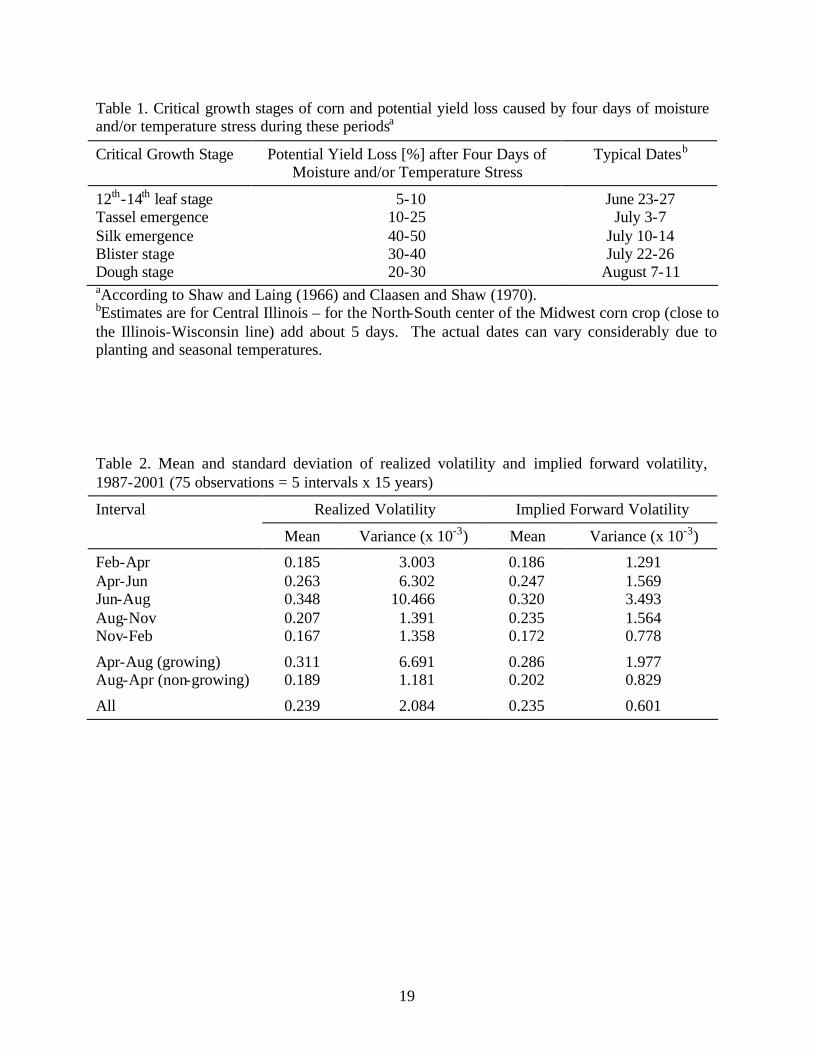
Buckle (1997) examine the implied forward volatilities as predictors of realized volatilities. Using one-month and two-month maturity American options on the FTSE 100 index from June 1993 to September 1995, they compare the implied forward volatility between the two expiration dates with the realized volatility over this period. The implied forward volatility is found to consistently overestimate realized volatility as evaluated by mean absolute and mean squared errors, and to have poor forecasting ability. Because Gwilym and Buckle’s (1997) data are limited to one-month and two-month options, the implied forward volatilities are constrained to one-month intervals, and hence no term structure unfolds. Further, no evaluation of other predictive properties such as the directional change of volatility is conducted. Specific Characteristics of the Corn Market An advantage of using a commodity such as corn to evaluate the implied forward volatilities as predictors of future realized volatility is that researchers (Roll, 1984; Anderson, 1985; and Kenyon et al., 1985) as well as market participants have observed repeating patterns of varying volatilities in agricultural futures markets. Anderson (1985), for example, finds strong seasonality in the volatility of corn, wheat, and soybean futures prices between 1969 and 1980. The periods of higher and lower volatility follow the growing and non-growing cycles of the crops. Corn is a determinant crop, which means the plant grows according to an internal clock and cannot generate new growth to compensate for stress during key growth periods. Hence, periods when moisture and temperature are especially critical to crop development are characterized by greater volatility than periods where weather has a less profound impact on crop growth and future yields. Times particularly critical to corn growth and the potential impact of four days of stress on yields are given in Table 1. The higher volatility during critical periods reflects the greater uncertainty and risk that market participants face during those intervals. As the crop passes through this time and the actual weather is observed, this uncertainty is gradually resolved and the volatility starts to decline. Since these critical growth periods repeat annually,
5
market participants know before the crop is planted the approximate times of greater corn price volatility. In an efficient options market, the implied forward volatilities that contain these growth periods are expected to be higher than for periods where weather has a less profound impact on crop development. Methods Volatility Estimates Following Fackler and King (1989) and Sherrick et al. (1996), this study assumes no-arbitrage conditions and uses Cox and Ross’ (1976) description of options premiums as the discounted expected future payoffs against a risk neutral valuation measure (RNVM) that characterizes the return distribution of the underlying asset. Under this approach the current premiums of European call and put options are given by
∫∞
−=0
)(),0max()()( TTTc dFFgxFTbxV [1]
∫∞
−=0
)(),0max()()( TTTp dFFgFxTbxV [2]
where Vc and Vp are the premiums of European call and put options, x is the options’ strike price, T is the time to expiration, FT is the price of the underlying asset at expiration, b(T) is the discount factor, and g(FT) is the market expected probability density function of the underlying asset price, FT, at maturity.5 If g(FT) is assumed to be lognormal, the relationship represents the Black-Scholes option pricing model. The observed option premiums and the current discount rate can be used to recover the implied RNVM, i.e. the distribution of the underlying asset price.
The approach differs from traditional Black-Scholes option pricing applications in two
ways. First, no restrictions are imposed on the asset distribution’s underlying mean, such as the mean equaling the current asset price or being a function thereof, or the underlying asset’s price process. The only assumption needed is that no-arbitrage conditions prevail. Second, in contrast to just using the option nearest to being at-the-money, the information contained in all calls and puts across all strike prices is used simultaneously.
The objective function used to recover the appropriate implied distribution is
−−+
−− ∑ ∫∑ ∫
==
∞ l
j
x
TTjTjp
k
i xTiTTic
j
i
dYYxYgTbVdYxYYgTbV1
2
0,
1
2
, ))(|()())(|()(min ϕϕϕ
[3]
5 In this paper we use a European options pricing model to approximate the American options price of the corn futures options.
6
where ϕ is the parameter vector for the particular distribution, Vc,i and Vp,j are the observed options premiums, xi and xj are the respective call or put strike prices, and k and l are the number of calls and puts for a particular day. Solving this equation for a specific options maturity yields the most suitable parameter vector. The RNVM can be approximated by a number of distributions. However, Fackler and King (1989) and Sherrick et al. (1996) find that there is little gain in accuracy by using distributions other than the traditional lognormal.
Since the approach yields a different parameter vector for each set of maturities, implied
volatilities can be recovered for different times to expiration. Assuming that variance is additive, those different implied volatilities can be used to calculate the implied forward volatility between two successive expiration dates, α−eT and eT , using
20,
20,, αα
σσσ−− −−− −=
eeee TivTivTTifv 0>α . [4]
The implied forward volatility represents the market’s expectation of the average volatility that will occur during this future interval (Figure 1). This expectation can be annualized as follows
( )ααα
σσ−
−− −×=
−−ee
TTifvTTIFV TTeeee
365,, . [5]
The realized volatility of the underlying futures contract, F, during the period between
two consecutive expiration dates is calculated on daily log returns
)/ln( 1−= ttt FFR . [6] Denoting D as the number of trading days in the interval, α−eT to eT , the mean return µ during this period is estimated by
D
RR
D
tt∑
== 0 , [7]
and the variance of Rt by
( )1
)(0
2
2
−
−=
∑=
D
RRv
D
tt
. [8]
However, in a perfectly efficient futures market R is zero, and hence the realized volatility is
7
D
RD
tt
TTreal ee
∑=
− =−
0
2
, ασ , [9]
which can be expressed in an annualized form by
365,, ×= −− −− eeee TTrealTTREAL αασσ . [10]
Forecast Evaluation Methods The predictive performance of the implied forward volatility is evaluated with respect to alternative predictors of future volatility in order to assess whether market participants incorporate new information into their volatility forecasts. The three-year moving average of past realized volatilities during the respective intervals and the naïve forecast defined as the volatility realized during the time interval in the previous year are chosen as alternative forecasts. Levels of Volatility The implied forward volatility and the alternative forecasts as predictors of future realized volatility are first examined using a simple regression framework
εσαασ ++= FORECASTREAL 10 [11] where REALσ and FORECASTσ refer to the annualized realized and forecasted volatilities. The forecasted volatilities are the implied forward volatility, the three-year moving average, or the naïve forecast. A significant coefficient 1α indicates that the forecast contains information about subsequent realized volatility. A significant constant term 0α indicates an average level of stochastic volatility that the market is unable to predict. In this context, an efficient or unbiased forecast is often characterized by 00 =α and 11 =α which can be tested using equation [11] with an F-test. The differences in accuracy of the three volatility forecasts are further evaluated based on relative forecast errors using the mean absolute percentage error (MAPE) and the mean squared percentage error (MSPE)
( )∑
− −
−−
− −
−− ×−
=ee ee
eeee
TT TTREAL
TTREALTTFORECAST
nMAPE
α α
αα
σ
σσ100
1
,
,, [12]
( )
∑− −
−−
− −
−−
×
−=
ee ee
eeee
TT TTREAL
TTREALTTFORECAST
nMSPE
α α
αα
σ
σσ2
,
,, 1001
. [13]
8
These error measures are then compared using the Modified Diebold Mariano (MDM) test proposed by Harvey, Leybourne, and Newbold, HLN (1997). The procedure involves specifying a cost-of-error function, g(e), of the forecast errors e and testing pair-wise the null hypothesis of equality of expected forecast performance. The test statistic, which HLN (1997) indicate should be compared with the critical values from the Student’s t distribution with (T – 1) degrees of freedom, is computed for one-step ahead forecasts as
( )d
ddT
TMDM T
tt∑
=
−
−=
1
211
, [14]
where dt =g(et,1)-g(et,2), d is the average difference across all years, and the null hypothesis is E(dt)=0. For example, when testing for significant differences of the MAPEs of two forecasts, g(et,1)=|et,1| is the absolute percent forecast error of method 1, g(et,2)=|et,2| is the absolute percent forecast error of method 2, and dt=et,1-et,2 is the difference between the respective absolute percent forecast errors at time t.
HLN (1998) demonstrate that the size of the MDM test is insensitive to contemporaneous
correlation between the forecast errors and that its power declines only marginally with departures from normality. They argue that these characteristics are important since researchers attempting to differentiate between forecasts are often faced with correlated forecasts that possess occasional large errors. This is also the case in our study. Other advantages of the MDM test include its applicability to multiple-step ahead forecast horizons, its non-reliance on an assumption of forecast unbiasedness, and its applicability to cost-of-error functions other than the conventional quadratic loss. HLN (1997) assert that the MDM test constitutes the “best available” method for determining the significance of observed differences in competing forecasts.
Changes in Volatility On a particular trading day, forward volatilities for successive time intervals can be extracted from the options prices. Hence, these premiums contain information about the market’s expectation of future volatilities and about the directional change of those future volatilities over time. For example, following the growing cycle of the crop and observing historical patterns of volatility, the implied forward volatility in the February-April interval might be lower than in April-June interval as the latter displays historically greater realized volatilities than the former. Hence, each trading day a term structure of the implied forward volatility unfolds that reflects not only trader’s expectations about the level of future volatility but also its directional change.
Following Henriksson and Merton (1981) and Henriksson (1984) the accuracy of
predicting directional change is evaluated using the log odds ratio in the regression
( )[ ]( )[ ] ( )iUiziz
100Pr1Pr
log ββ +=
==
[15]
9
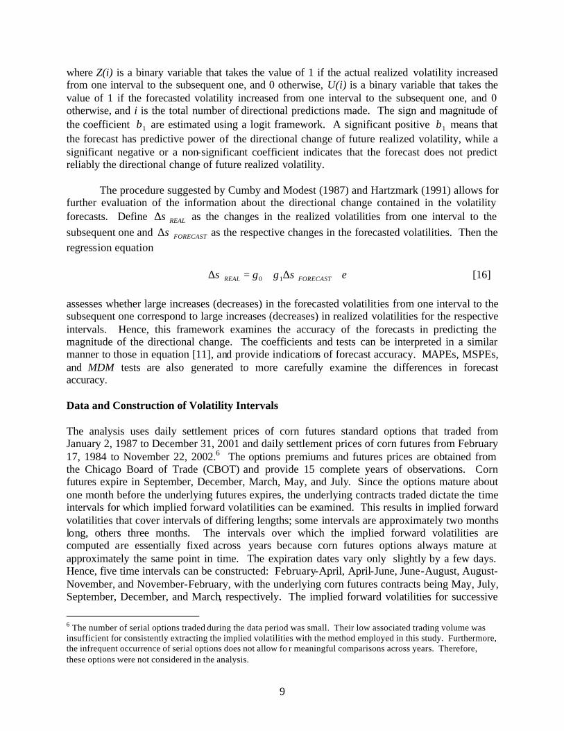
where Z(i) is a binary variable that takes the value of 1 if the actual realized volatility increased from one interval to the subsequent one, and 0 otherwise, U(i) is a binary variable that takes the value of 1 if the forecasted volatility increased from one interval to the subsequent one, and 0 otherwise, and i is the total number of directional predictions made. The sign and magnitude of the coefficient 1β are estimated using a logit framework. A significant positive 1β means that the forecast has predictive power of the directional change of future realized volatility, while a significant negative or a non-significant coefficient indicates that the forecast does not predict reliably the directional change of future realized volatility.
The procedure suggested by Cumby and Modest (1987) and Hartzmark (1991) allows for
further evaluation of the information about the directional change contained in the volatility forecasts. Define REALσ∆ as the changes in the realized volatilities from one interval to the subsequent one and FORECASTσ∆ as the respective changes in the forecasted volatilities. Then the regression equation
εσγγσ +∆+=∆ FORECASTREAL 10 [16]
assesses whether large increases (decreases) in the forecasted volatilities from one interval to the subsequent one correspond to large increases (decreases) in realized volatilities for the respective intervals. Hence, this framework examines the accuracy of the forecasts in predicting the magnitude of the directional change. The coefficients and tests can be interpreted in a similar manner to those in equation [11], and provide indications of forecast accuracy. MAPEs, MSPEs, and MDM tests are also generated to more carefully examine the differences in forecast accuracy. Data and Construction of Volatility Intervals The analysis uses daily settlement prices of corn futures standard options that traded from January 2, 1987 to December 31, 2001 and daily settlement prices of corn futures from February 17, 1984 to November 22, 2002.6 The options premiums and futures prices are obtained from the Chicago Board of Trade (CBOT) and provide 15 complete years of observations. Corn futures expire in September, December, March, May, and July. Since the options mature about one month before the underlying futures expires, the underlying contracts traded dictate the time intervals for which implied forward volatilities can be examined. This results in implied forward volatilities that cover intervals of differing lengths; some intervals are approximately two months long, others three months. The intervals over which the implied forward volatilities are computed are essentially fixed across years because corn futures options always mature at approximately the same point in time. The expiration dates vary only slightly by a few days. Hence, five time intervals can be constructed: February-April, April-June, June-August, August-November, and November-February, with the underlying corn futures contracts being May, July, September, December, and March, respectively. The implied forward volatilities for successive
6 The number of serial options traded during the data period was small. Their low associated trading volume was insufficient for consistently extracting the implied volatilities with the method employed in this study. Furthermore, the infrequent occurrence of serial options does not allow fo r meaningful comparisons across years. Therefore, these options were not considered in the analysis.
10
two-month and three-month intervals can be chronologically stacked. In this manner, a complete and continuous term structure of future volatilities emerges reaching from approximately 6 months up to 12 months into the future, depending on the available maturities of the options traded.
The lognormal distribution is used as the RNVM to extract the implied volatilities from
the corn options premiums. This distribution has been shown to work reasonably well for obtaining the implied volatilities from soybean futures options (Fackler and King, 1989; Sherrick et al., 1996). Furthermore, the lognormal distribution allows for greater degrees of freedom than higher-order distributions because it requires only a two-parameter ϕ vector. The discount factor b(T) is calculated by compounding the corresponding three-month T-Bill rate obtained from the Federal Reserve Board over the time to maturity of the options.
The data are first screened to exclude options that are listed, but did not actually trade;
block trades; and options violating monotonic strike-premium patterns. Furthermore, a minimum of three valid observations is required for each set of options because the parameter vector of the lognormal distribution contains two elements, and using only two observations would yield a system of two equations with two unknowns resulting in a perfect fit with no error. Sets of options consisting entirely of calls or puts are excluded from the analysis as those sets are frequently inconsistent with monotonic volatility patterns. The remaining options in each set are equally weighted when computing the implied volatility using Equation [3]. Finally, the annualized forward volatilities implied by two sets of subsequent options are obtained using Equation [5]. The implied forward volatilities are extracted from sets of options that traded 2 months before the beginning of the interval, i.e. 2 months before the expiration of the options with the shorter maturity. Because the time intervals are either two or three months long, this approach assures non-overlapping observations.
The realized futures price volatilities are calculated using equation [10]. The annualized
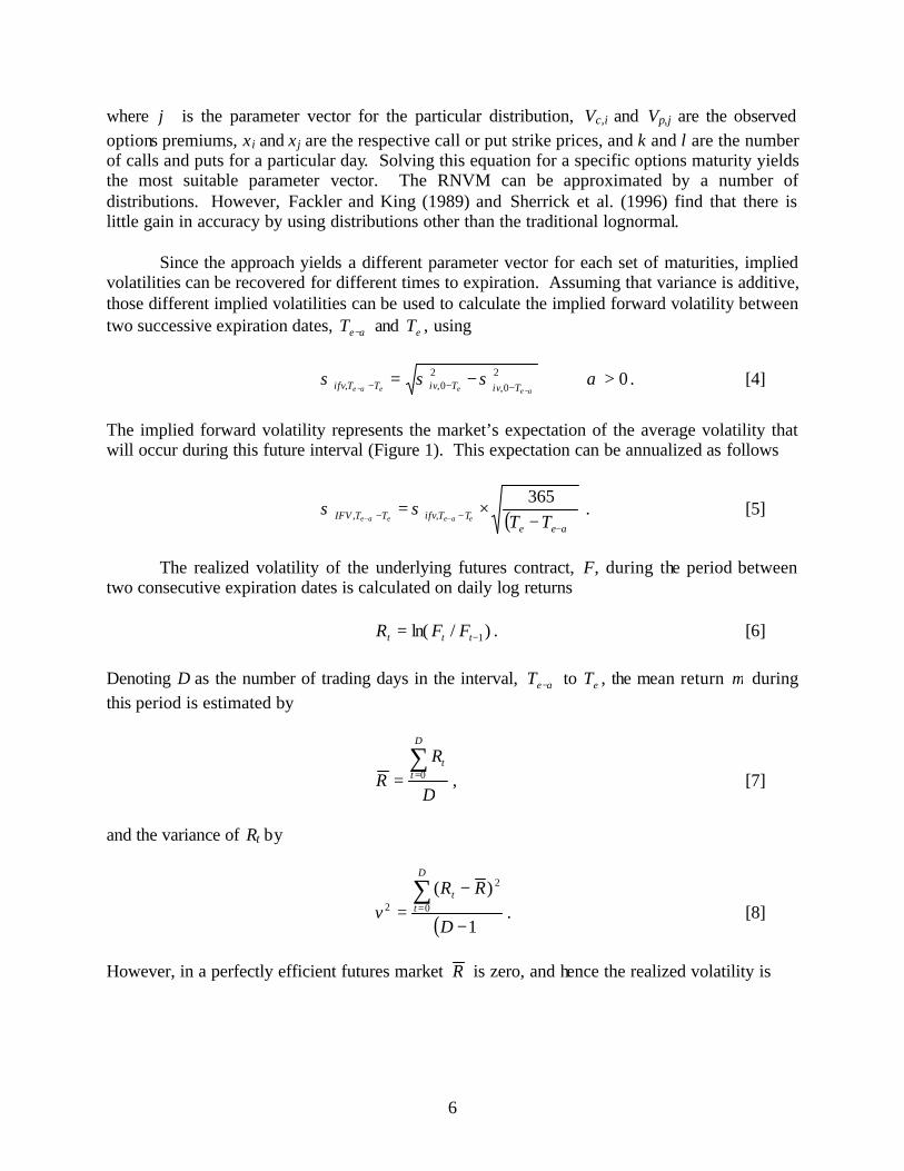
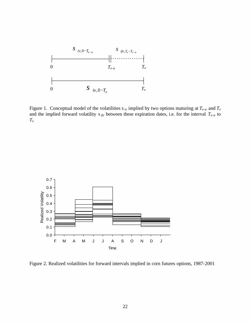
volatilities for the corresponding time intervals are based on the contracts underlying the set of options with the longer time to maturity and are computed around an assumed mean of zero (Equation [9]). Two reasons warrant this approach. First, in an efficient futures market, no arbitrage requires that the mean return from holding futures contracts is zero. Second, Figlewski (1997) cautions that when dealing with short sample periods as is the case in this study, noisy price movements can result in deviations from the true mean and make the estimate, R , very inaccurate. Since the options mature about one month before the futures, all problems usually associated with prices close to maturity of a futures contract are avoided because that period is automatically excluded when calculating the realized volatility. This treatment is important as the time right before the expiration of the futures is usually characterized by high volatility often attributed to traders closing positions to avoid delivery. Analysis and Results General Pattern The realized volatilities for the five intervals are displayed in Figure 2. The graph shows the anticipated repeating patterns of varying volatilities in the corn futures market. The April-June
11
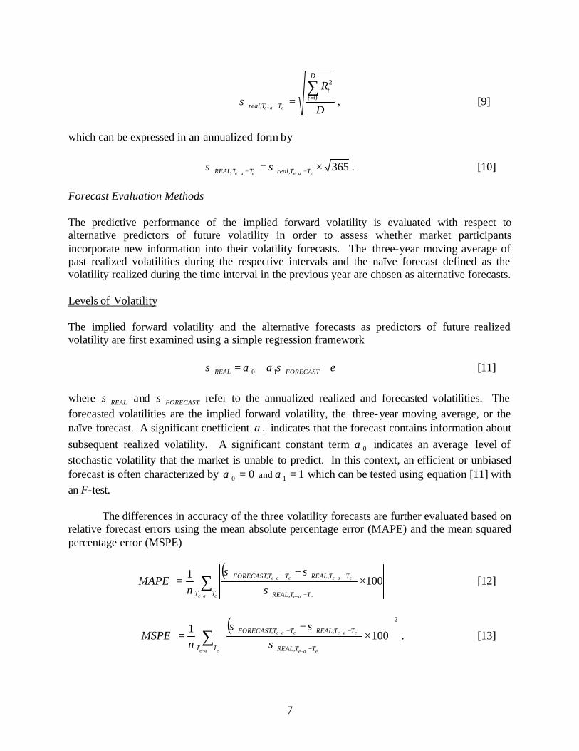
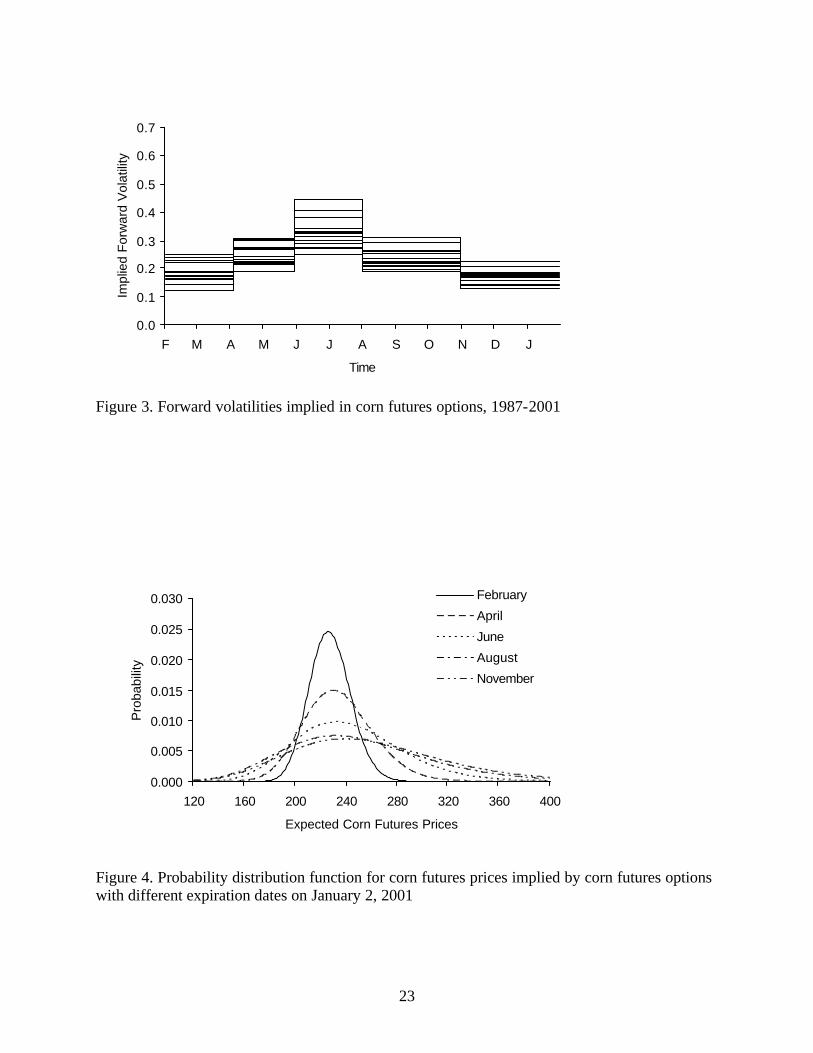
and June-August intervals that cover the majority of the growing cycle tend to display the largest volatilities (Table 2). As the effect of weather uncertainty is the largest during the April-June and June-August intervals, the associated volatility is greater in those intervals than in the harvest interval (August-November) and the storage intervals (November-February and February-April) where weather has less or no impact. The average realized volatility during the growing period exceeds the average volatility of the non-growing period (0.311 vs. 0.189; pt-test,
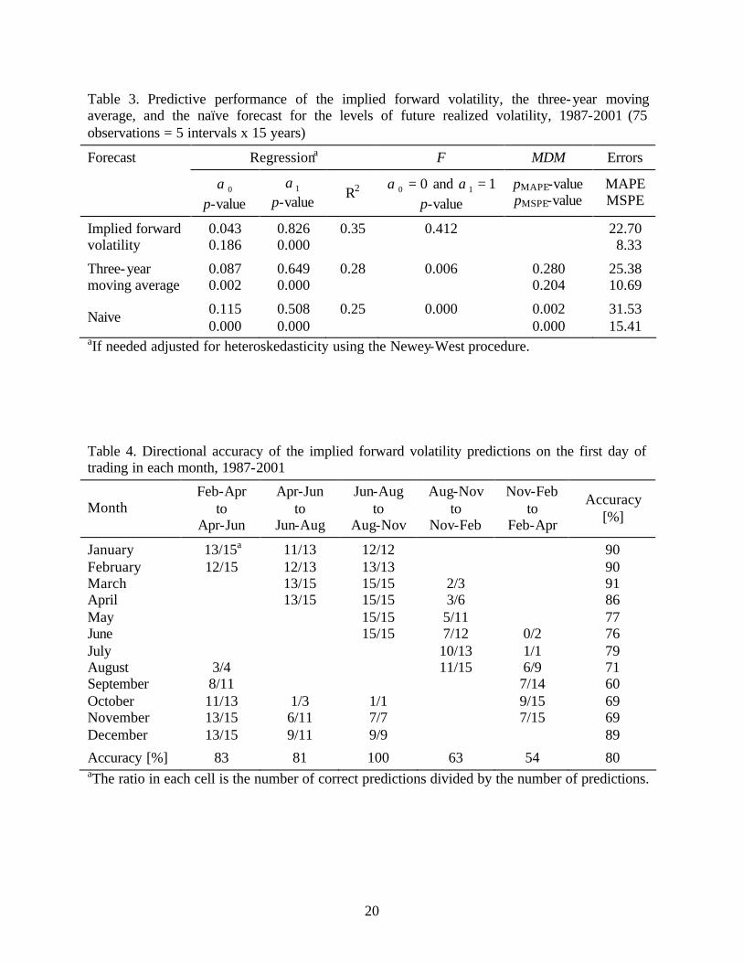
pairwise=0.000) and also displays a greater variance of those volatilities (6.691 x 10⁻³ vs. 1.181 x 10⁻³; pF-test=0.001). Furthermore, during the growing cycle, weather tends to cause more uncertainty during the June-August interval than during the April-June interval (0.348 vs. 0.263; pt-test , pairwise=0.002) because the former contains the more critical periods for crop development (Table 1). The differences in volatility between growing and non-growing intervals and within the growing interval confirm the findings of Anderson (1985). The repeating volatility patterns observed for the realized volatilities are also reflected in the implied forward volatilities (Figure 3). Overall, the graph shows that market participants incorporate the greater impact of weather on corn futures prices during the growing period than during the non-growing period (0.286 vs. 0.202; pt-test , pairwise=0.000). As observed for the realized volatilities, the variance of the implied forward volatilities for the growing period is also greater than during the non-growing period (1.977 x 10⁻³ vs. 0.829 x 10⁻³; pF-test=0.058). Moreover, the implied forward volatilities for the June-August interval are greater than those for the April-June interval (0.320 vs. 0.247; pt-test, pairwise=0.000) indicating that the respective uncertainty associated with the critical growing periods in each time interval is incorporated in options prices. Predictive Performance in Levels The explanatory power of the implied forward volatility and the alternative forecasts regarding future realized volatility is first evaluated with equation [11].7 Differences in forecast accuracy are then examined using the MDM tests. The analysis is based on 75 observations as there are 5 two- and three-month intervals in each of the 15 years. The results in Table 3 show that in terms of R2, the implied forward volatility provides modestly better predictions of future realized volatility (R2=0.35) than the three-year moving average (R2=0.28) and the naïve forecast (R2=0.25). The coefficient estimates for 1α are significant for all forecasts indicating that all have significant explanatory power of future realized volatility. The constant term is not significant for the implied forward volatility (p=0.186). In contrast, the constant is significant for the alternative forecasts. Furthermore, the joint hypothesis 00 =α and 11 =α is rejected by an F-test for the alternative forecasts, but not for the implied forward volatility indicating that the implied forward volatility is a more effective forecast, capturing a larger portion of the systematic variability in the realized volatility.
The magnitude of the forecast errors as measured by the MAPE and MSPE is larger for
alternative forecasts than for the implied forward volatility. These differences are evaluated using the MDM test. The error function g(e) is specified as the absolute percent forecast error
7 To conserve observations, the moving averages for the intervals in 1987-1989 are obtained using 1984-1986 corn futures data.
12
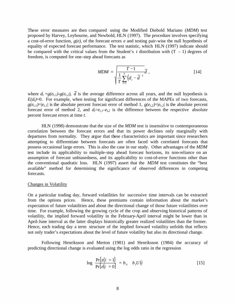
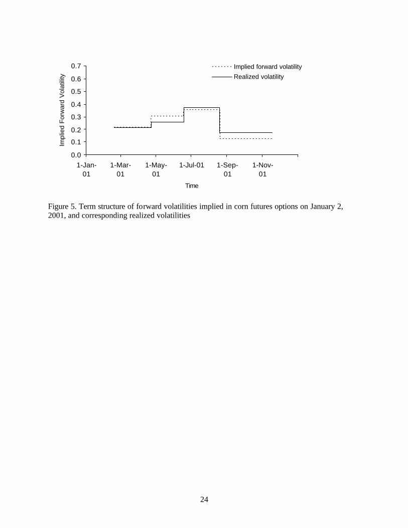
and the squared percent forecast error and tests for statistical significance in the differences of the MAPEs and the MSPEs between the implied forward volatility and each alternative forecast. Significant differences are found for both specifications of the error function in tests between the implied forward volatility and the naïve forecast (Table 3). The differences between the implied forward volatility and the three-year moving average are not significant . These findings indicate that larger differences in forecast ability emerge when less past information is incorporated into making the forecast. Predictive Performance in Changes The term structure of the implied forward volatility is examined for the first trading day of each month. Depending on the expiration dates of the options traded on the first trading day of each month the term structure of forward volatility varies in length within and across years. For example, on January 2, 2001, five option maturities were traded: February, April, June, August, and November. Figure 4 depicts the corresponding distributions implied by these options. The differences in the distributions express the market’s expectation of how the uncertainty in the corn futures market will be resolved over time. The smaller variance of the close-to-maturity options indicates that little uncertainty remains regarding the nearby futures price. The greater variance of the longer-term options reflects the market’s increasing uncertainty regarding the futures price at more distant times. From the five different implied volatilities, the implied forward volatilities for four consecutive intervals, February-April, April-June, June-August, and August-November, can be obtained. The term structure implied by these forward volatilities and the corresponding realized vo latilities for each of those intervals are displayed in Figure 5.8 The small difference in variance between the options expiring in August and in November observed in Figure 4, for example, translates into a small implied forward volatility for the August-November interval in Figure 5, and indicates that market participants expect most of the uncertainty regarding the corn futures price to be resolved by August. Term Structure Implied Across Months The forecasting ability of the implied forward volatilities regarding the directional change from one time interval to the next is first examined by assessing the number of correct directional predictions. In the example of 2001, the implied forward volatilities predict accurately the term structure of the realized volatilities – two successive increases in volatility over the growing intervals followed by a decrease during the harvest interval (Figure 5). Table 4 summarizes the directional accuracy of the implied forward volatility predictions. Vertically, the table illustrates how with successive months the market adds new intervals, so that at each point in time forecasts for several subsequent future intervals are available. On average the implied forward volatilities predict the directional change of the realized volatilities correctly in about 80% of the cases with percentages of correct directional predictions ranging from 60% on the first trading day in September to 91% on the first trading day in March. Table 4 also shows the tendency of the market to provide fewer volatility forecasts for more distant intervals, particularly in August, September, and October. The smaller number of forecasts is a sign of the reduced activity in
8 Note that Figures 4 and 5 are complements, as jointly they capture all information regarding the expected future volatility available from the options prices.
13
options with longer expirations. With reduced trading activity, these more distant options may contain less market information.
Market participants have a better ability to correctly forecast the directional change
earlier in the calendar year: from the second storage interval to the first growing interval (83%); from the first growing interval to the second growing interval (81%); and from the second growing interval to the harvest interval (100%). In contrast, later in the calendar year when volatility differences between the intervals are less pronounced the ability to predict the differences declines: from the harvest interval to the first storage interval (63%); and from the first storage interval to the second storage interval (54%). The high degree of accuracy in predicting the directional change in volatility from the second growing interval to the harvest interval expresses the market’s expectation that most of the weather related uncertainty regarding the final crop size is resolved by mid-August. This result is consistent with recent findings by Egelkraut et al. (2003) who evaluate the accuracy of crop production forecasts provided by USDA and two private information agencies for corn and soybeans and find that the corn forecasts released in early August are good predictors of final crop size. Simply put, less supply uncertainty remains to be resolved during the harvest period.
Term Structure Implied in January and August The term structure of the implied forward volatility is analyzed more closely for January and August. These months represent important times for participants in the corn market. January is the first month of the new crop year, and farmers typically make planting decisions at that time in order to have sufficient time to arrange financing and to obtain supplies such as seeds, herbicides, and fertilizer. In contrast, by August most of the uncertainty regarding the size of the current corn crop is resolved (Egelkraut et al., 2003) and market participants begin to evaluate alternative marketing strategies. Therefore, information about future volatility becomes particularly important in these months.
The term structure extracted on the first trading day in January covers four intervals, the
second storage interval, the first and second growing intervals, as well as the harvest interval (Table 4). The accuracies of the predictions of the directions of future volatility changes from one of those intervals to the next are 87%, 85%, and 100% respectively with a mean of 90%. On the first trading day in August, the implied term structure extends over the harvest interval, the first and second storage interval, and the first growing interval. The directional change of future volatility is less accurate, predicting correctly 73%, 67%, and 75% respectively with a mean of 71%.
The predictive performance of the implied forward volatility and the alternative forecasts
of the directional change of future realized volatility is evaluated with equation [15]. The coefficient estimates for 1β are significantly greater than zero for all forecasts with the exception of the naïve forecast in August suggesting that these forecasts contain information about the directional change of future realized volatility (Table 5). Furthermore, all forecasts perform better in January than in August because of the more consistent volatility pattern over the growing period than over the non-growing period. Usually, two consecutive increases in volatility from the second storage interval to the first and further to the second growing interval
14
are followed by a decrease from the second growing interval to the harvest interval. However, in August where the volatility pattern extending over the non-growing period is less regular, less accuracy and statistical differences may exist. Overall, the three forecasts appear to predict the direction of change of future realized volatility rather well, but based on the percentage accuracy of the predictions and p-values it appears that the implied forward volatilities and the three-year moving average forecast perform just about the same which is superior to the naïve forecast.
Analyzing the magnitude of change in future volatility using equation [16], we find that
for both months, the constant term is insignificant and 1γ is significantly positive for all forecasts (Table 6), demonstrating that forecasts contain information about the magnitude of the change. In two cases, however, the joint hypothesis 00 =γ and 11 =γ is rejected, indicating that the naïve forecast in January (p=0.021) and the implied forward volatility in August (p=0.006) are biased. In these cases, the magnitudes of the coefficients suggest that the implied forward volatilities overstate realized volatilities. In evaluating the statistical differences in the forecasts, the implied forward volatility and the two alternative forecasting methods are not expected to significantly differ in January because the volatility pattern that prevails over the crop year is rather well established. The findings displayed in Table 6 are fairly consistent with this expectation. The MDM test provides only a modest indication of a significant difference between the forecasts in January. In August, the three-year moving average performs most effectively; the results of the MDM test indicate significant differences between the implied forward volatility and the three-year moving average. No differences exist between the implied forward volatility and the naïve forecast. Hence, even though the implied forward volatility performs equally well in predicting the directional change of future volatility in August, it does not incorporate as well past information about the magnitude of this change. The decline of the predictive performance of the implied forward volatilities relative to the three-year moving average in August is likely related to the less pronounced pattern of volatility in the non-growing intervals, and the reduced number of options traded at more distant intervals during this period. Fewer transactions reflect a lower informational content in the market. Summary and Conclusion This paper identifies the information and procedures to develop the term structure of volatility implied by option prices, and evaluates the informational content of the implied forward volatility as a predictor of subsequent realized price volatility in the corn futures market. Using 15 years of options and futures prices, two types of information are generated: 1) the market’s estimate of future realized volatility during the nearby interval of the term structure, and 2) the market’s expectation of the direction and magnitude of change of future realized volatility over time. For each information set, comparisons of the predictive accuracy are based on the ability of implied forward volatility to explain subsequent realized volatility. Further, mean squared percentage errors (MSPEs), mean absolute percentage errors (MAPEs), and the Modified Diebold Mariano (MDM) test are used to assess the accuracy of the implied forward volatility against forecasts generated from historical volatility. We also assess the ability of the forecasts to reflect the direction of change in realized volatility. The results indicate that the implied forward volatility reflects rather well the general pattern of realized volatility in the corn market. Based on the information for the nearby interval of the term structure, our findings indicate that the implied forward volatility provides unbiased forecasts and captures a larger portion of the
15
systematic variability in the realized volatility than the forecasts based on historical information. The comparison to the three-year moving average and the naïve forecast suggests a modestly better performance of the implied forward volatility as measured by the larger R2 and the smaller MAPEs and MSPEs. Results from the MDM tests of the statistical differences in the forecasts reinforce the modest superiority of the implied forward volatility. Using the information on the direction and magnitude of change in volatility, we find that the early-year options predict about equally well as the three-year moving average and better than the naïve forecast. Later-year options and alternative forecast procedures are less able to predict the direction of changing volatility, but the implied forward volatility and the three-year moving average forecast appear to be marginally better than the naïve forecast. During this later-year period, the three-year moving average forecast of the magnitude of the change in variability outperforms the forecasts from the implied forward volatility which tend to over-predict.
Our findings are in contrast to Gwilym and Buckle (1997) who, analyzing FTSE 100
index options, find insignificant coefficients for the implied forward volatility and significant coefficients for the constant term and conclude that the implied forward volatility has limited predictive power. For corn, the implied forward volatility does explain the variability of future realized volatility. Further, in most cases the implied forward volatility provides forecasts that are marginally better than or equal to forecasts generated from historical volatilities. In contrast to Gwilym and Buckle (1997) we find only limited evidence of systematic over-predictions by the implied forward volatility. The source of the over-predictions may be related to the less pronounced pattern of volatility in the non-growing intervals, and the reduced number of options traded at more distant intervals during this period. With reduced trading activity, these more distant options may contain less market information.
The results of our analysis can also be interpreted within the traditional mean-reversion
framework of volatility (employed for example by Stein (1989) and Xu and Taylor (1994)). Instead of considering the volatility behavior around a long-run mean as essentially random, we identify a reoccurring, systematic pattern of volatility that is closely related to the specific characteristics of the underlying commodity. Since market participants incorporate this volatility pattern into prices, options contain more information than just the average volatility. This additional information expresses the market’s expectation about the time and size of positive and negative deviations from the implied mean volatility.
While previous research by Gwilym and Buckle (1997) indicates that the implied forward
volatility may not be a good predictor of price variability in financial assets, the approach appears to hold promise in agricultural markets. For corn, we find that the implied forward volatility performs reasonably well in forecasting realized volatility. Future research should extend this analysis to other commodities such as soybeans and wheat and further investigate the value of the implied forward volatility for agriculture.
16
References Anderson, R. “Some Determinants of the Volatility of Futures Prices.” Journal of Futures Markets 5(1985):331-348. Black, F., and M. Scholes. “The Pricing of Options and Corporate Liabilities.” Journal of Political Economy 81(1973):637-659. Black, F. “Studies of Stock Price Volatility Changes.” In: Proceedings of the 1976 Meetings of the American Statistical Association, Business and Economic Statistical Section (1976):177-181. Campa, M. and K. Chang. “Testing the Expectations Hypothesis on the Term Structure of Volatilities in Foreign Exchange Options.” Journal of Finance 50(1995):529-547. Canina, L., and S. Figlewski. “The Informational Content of Implied Volatility.” Review of Financial Studies 6(1993):659-681. Christensen, B. J., and N. R. Prabhala. “The Relation between Implied and Realized Volatility. ” Journal of Financial Economics 50(1998):125-150. Claasen, M. M., and R. H. Shaw. “Water Deficit Effects on Corn II. Grain Components.” Agronomy Journal 62(1970):652-655. Cox, J. C., and S. A. Ross. “The Valuation of Options for Alternative Stochastic Processes.” Journal of Financial Economics 3(1976):145-166. Cumby, R. E., and D. M. Modest. “Testing for Market Timing Ability.” Journal of Financial Economics 19(1987):169-189. Day, T. E., and C. M. Lewis. “Stock Market Volatility and the Information Content of Stock Index Options.” Journal of Econometrics 52(1992):267-287. Day, T. E., and C. M. Lewis. “Forecasting Futures Market Volatility.” Journal of Derivatives 1(1993):33-50. Ederington, L. H., and W. Guan. “Forecasting Volatility.” Working Paper (2000), University of Oklahoma. Egelkraut, T. M., P. Garcia, S. H. Irwin, and D. L. Good. “An Evaluation of Crop Forecast Accuracy for Corn and Soybeans: USDA and Private Information Agencies.” Journal of Agricultural and Applied Economics 35(2003):79-95. Fackler, P. L., and R. P. King. “Calibration of Option-Based Probability Assessments in Agricultural Commodity Markets.” American Journal of Agricultural Economics 72(1989):73-83.
17
Fama, E. F. “The Behavior of Stock Market Prices.” Journal of Business 38(1965):34-105. Feinstein, S. P. “Forecasting Stock Market Volatility using Options on Index Futures.” Economic Review, Federal Reserve Bank of Atlanta 74(1989):12-30. Figlewski, S. “Forecasting Volatility.” Financial Markets. Institutions and Instruments 6(1997):1-88. Fleming, J. “The Quality of Market Volatility Forecasts Implied by S&P 100 Index Option Prices.” Journal of Empirical Finance 5(1998):317-345. French, K. R., G. W. Schwert, and R. F. Stambaugh. “Expected Stock Returns and Volatility.” Journal of Financial Economics 19(1987):3-30. Geske, R. “A Note on an Analytical Valuation Formula for Unprotected American Call Options on Stocks with Known Dividends.” Journal of Financial Economics 7(1979):375-380. Gwilym, O. and M. Buckle. “Forward/Forward Volatilities and the Term Structure of Implied Volatility.” Applied Economics Letters 4(1997):325-328. Hartzmark, M. L. “Luck versus Forecast Ability: Determinants of Trader Performance in Futures Markets.” Journal of Business 64(1991):49-74. Harvey, D., S. Leybourne, and P. Newbold. “Testing the Equality of Prediction Mean Squared Errors.” International Journal of Forecasting 13(1997):281-291. Harvey, D., S. Leybourne, and P. Newbold. “Tests for Forecast Encompassing.” Journal of Business & Economic Statistics 16(1998):254-259. Henriksson, R. D. “Market Timing and Mutual Fund Performance.” Journal of Business 57(1984):73-96. Henriksson, R. D., and R. C. Merton. “On Market Timing and Investment Performance. II. Statistical Procedures for Evaluating Forecasting Skills.” Journal of Business 54(1981):513-533. Hull, J., and A. White. “The Pricing of Options on Assets with Stochastic Volatilities.” Journal of Finance 42(1987):281-300. Johnson, H., and D. Shanno. “Option Pricing when the Variance is Changing.” Journal of Financial and Quantitative Analysis 22(1987):143-151. Jorion, P. “Predicting Volatility in the Foreign Exchange Market.” Journal of Finance 50(1995):507-528.
18
Kenyon, D., K. Kling, J. Jordon, W. Seale, and N. McCable. “Factors Affecting Agricultural Futures Price Volatility.” Dep. Agr. Econ. Staff Pap. No. 85-14, Virginia Polytechnic Institute and State University, Aug. 1985. Lamoureux, C., and W. Lastrapes. “Forecasting Stock-Return Variance: Toward an Understanding of Stochastic Implied Volatilities.” Review of Financial Studies 6(1993):369-381. Merton, R. C. “Theory of Rational Option Pricing.” Bell Journal of Economics and Management Science 4(1973):141-183. Merton, R. C. “On Estimating the Expected Return on the Market: An Explanatory Investigation.” Journal of Financial Economics 8(1980):323-362. Poterba, J., and L. Summers. “The Persistence of Volatility and Stock Market Fluctuations.” American Economic Review 76(1986):1141-1151. Roll, R. “An Analytic Valuation Formula for Unprotected American Call Options on Stocks with Known Dividends.” Journal of Financial Economics 5(1977):251-258. Roll, R. “Orange Juice and Weather.” American Economic Review 74(1984):861-880. Scott, L. “Option Pricing when the Variance Changes Randomly: Theory, Estimation, and an Application.” Journal of Financial and Quantitative Analysis 22(1987):419-438. Shaw, R. H., and D. R. Laing. “Moisture Stress and Plant Response.” In: Plant Environment and Efficient Water Use, Agronomy Society of America, Madison, Wisconsin (1966):73-94. Sherrick, B., P. Garcia, and V. Tirupattur. “Recovering Probabilistic Information from Option Markets: Tests of Distributional Assumptions.” Journal of Futures Markets 16(1996):545-560. Stein, J. “Overreactions in the Options Market.” Journal of Finance 44(1989):1011-1023. Whaley, R. “On the Valuation of American Call Options on Stocks with Known Dividends.” Journal of Financial Economics 10(1981):29-58. Wiggens, J. “Options Values under Stochastic Volatility.” Journal of Financial Economics 19(1987):351-372. Xu, X., and S. J. Taylor. “The Term Structure of Volatility Implied by Foreign Exchange Options.” Journal of Financial and Quantitative Analysis 29(1994):57-74. Xu, X., and S. J. Taylor. “Conditional Volatility and the Informational Efficiency of the PHLX Currency Options Market.” Journal of Banking and Finance 19(1995):803-821.
19
Table 1. Critical growth stages of corn and potential yield loss caused by four days of moisture and/or temperature stress during these periodsa
Critical Growth Stage Potential Yield Loss [%] after Four Days of Moisture and/or Temperature Stress
Typical Datesb
12th-14th leaf stage Tassel emergence Silk emergence Blister stage Dough stage
5-10 10-25 40-50 30-40 20-30
June 23-27 July 3-7
July 10-14 July 22-26
August 7-11 aAccording to Shaw and Laing (1966) and Claasen and Shaw (1970). bEstimates are for Central Illinois – for the North-South center of the Midwest corn crop (close to the Illinois-Wisconsin line) add about 5 days. The actual dates can vary considerably due to planting and seasonal temperatures. Table 2. Mean and standard deviation of realized volatility and implied forward volatility, 1987-2001 (75 observations = 5 intervals x 15 years)
Interval Realized Volatility Implied Forward Volatility
Mean Variance (x 10-3) Mean Variance (x 10-3)
Feb-Apr Apr-Jun Jun-Aug Aug-Nov Nov-Feb
0.185 0.263 0.348 0.207 0.167
3.003 6.302 10.466 1.391 1.358
0.186 0.247 0.320 0.235 0.172
1.291 1.569 3.493 1.564 0.778
Apr-Aug (growing) Aug-Apr (non-growing)
0.311 0.189
6.691 1.181
0.286 0.202
1.977 0.829
All 0.239 2.084 0.235 0.601
20
Table 3. Predictive performance of the implied forward volatility, the three-year moving average, and the naïve forecast for the levels of future realized volatility, 1987-2001 (75 observations = 5 intervals x 15 years)
Forecast Regressiona F MDM Errors
0α p-value
1α p-value
R2 00 =α and 11 =α p-value
pMAPE-value pMSPE-value
MAPE MSPE
Implied forward volatility
0.043 0.186
0.826 0.000
0.35
0.412 22.70
8.33
Three-year moving average
0.087 0.002
0.649 0.000
0.28
0.006
0.280 0.204
25.38 10.69
Naive 0.115 0.000
0.508 0.000
0.25
0.000
0.002 0.000
31.53 15.41
aIf needed adjusted for heteroskedasticity using the Newey-West procedure. Table 4. Directional accuracy of the implied forward volatility predictions on the first day of trading in each month, 1987-2001
Month Feb-Apr
to Apr-Jun
Apr-Jun to
Jun-Aug
Jun-Aug to
Aug-Nov
Aug-Nov to
Nov-Feb
Nov-Feb to
Feb-Apr
Accuracy [%]
January February March April May June July August September October November December
13/15a 12/15
3/4 8/11 11/13 13/15 13/15
11/13 12/13 13/15 13/15
1/3 6/11 9/11
12/12 13/13 15/15 15/15 15/15 15/15
1/1 7/7 9/9
2/3 3/6 5/11 7/12 10/13 11/15
0/2 1/1 6/9 7/14 9/15 7/15
90 90 91 86 77 76 79 71 60 69 69 89
Accuracy [%] 83 81 100 63 54 80 aThe ratio in each cell is the number of correct predictions divided by the number of predictions.
21
Table 5. Predictive performance of the implied forward volatility, the three-year moving average, and the naïve forecast in January (40 observations) and in August (28 observations) for the directional change in future realized volatility, 1987-2001
Forecast January August
0β p-value
1β p-value
Accuracy [%]
0β p-value
1β p-value
Accuracy [%]
Implied forward volatility
-2.485 0.018
4.234 0.000
88
-1.012 0.089
1.705 0.048
68
Three-year moving average
-2.485 0.018
4.234 0.000
88
-1.099 0.062
2.079 0.022
71
Naive -1.012 0.087
2.398 0.002
78
-0.693 0.214
1.030 0.208
61
Table 6. Predictive performance of the implied forward volatility, the three-year moving average, and the naïve forecast in January (40 observations) and in August (28 observations) for the magnitude of change of future realized volatility, 1987-2001
Forecast January August
0γ p-value
1γ p-value
R2 pMAPE pMSPE
0γ p-value
1γ p-value
R2 pMAPE pMSPE
Implied forward volatility
0.010 0.576
0.870 0.000
0.36 0.003
0.786 0.475 0.006
0.26
Three-year moving average
-0.013 0.465
0.951 0.000
0.41
0.278 0.271
0.002 0.831
0.790 0.000
0.40
0.020 0.037
Naive -0.003 0.893
0.470 0.016
0.14
0.076 0.102
-0.003 0.768
0.641 0.001
0.36
0.252 0.266
22
Figure 1. Conceptual model of the volatilities s iv implied by two options maturing at Te-α and Te and the implied forward volatility s ifv between these expiration dates, i.e. for the interval Te-α to Te
0.0
0.1
0.2
0.3
0.4
0.5
0.6
0.7
F M A M J J A S O N D J
Time
Rea
lized
Vol
atili
ty
Figure 2. Realized volatilities for forward intervals implied in corn futures options, 1987-2001
ασ
−− eTiv 0, α
σ−− ee TTifv ,
eTiv −0,σ
0
0
Te-α Te
Te
23
0.0
0.1
0.2
0.3
0.4
0.5
0.6
0.7
F M A M J J A S O N D J
Time
Impl
ied
For
war
d V
olat
ility
Figure 3. Forward volatilities implied in corn futures options, 1987-2001
0.000
0.005
0.010
0.015
0.020
0.025
0.030
120 160 200 240 280 320 360 400
Expected Corn Futures Prices
Pro
babi
lity
February
April
June
August
November
Figure 4. Probability distribution function for corn futures prices implied by corn futures options with different expiration dates on January 2, 2001
24
0.0
0.1
0.2
0.3
0.4
0.5
0.6
0.7
1-Jan-01
1-Mar-01
1-May-01
1-Jul-01 1-Sep-01
1-Nov-01
Time
Impl
ied
For
war
d V
olat
ility
Implied forward volatility
Realized volatility
Figure 5. Term structure of forward volatilities implied in corn futures options on January 2, 2001, and corresponding realized volatilities