The Taylor Center:taylorcenter.org/Gofen/TaylorUserManual.doc · Web view3.1.6.1 Visualizing...

Alexander Gofen

The Taylor Center User Manual

All-in-One Interactive Integratorfor Ordinary Differential Equationsusing the Modern Taylor Method

Integration with the Highest Accuracy 2D or 3D Stereo Graphing

Real Time AnimationExploration

Version 31.0 for Windows®

2001-2020 © Alexander Gofen

San Francisco, USAMay 2020

5/20/2023 The Taylor Center User Manual for Windows Version 31.02

Brook Taylor 1685-1731

Introduced the Taylor expansion - the main foundation of differential calculus - in words

of J. L. Lagrange

Louis François Antoine Arbogast1759-1803

Introduced the main formulas for n-order derivatives including what was later named the

Faa di-Bruno formula.

List of Content

1. THE MODERN TAYLOR METHOD PACKAGE HIGHLIGHTS....................................8

1.1. Limitations of the method........................................................................................................................... 121.1.1. Holomorphy and elementariness of the right hand sides.........................................................................121.1.2. Non-stiff initial value problems............................................................................................................. 12

2. A QUICK TOUR.........................................................................................................13

2.1. Installation................................................................................................................................................... 13

2.2. Playing with the DEMO.............................................................................................................................. 14

2.3. Doing it by steps.......................................................................................................................................... 15

3. HOW TO RUN AND USE THE TAYLOR CENTER...................................................17

3.1. The Input..................................................................................................................................................... 183.1.1. Special input and processing of 2nd degree multivariate polynomials......................................................22

5/20/2023 The Taylor Center User Manual for Windows Version 31.0 3

3.1.1.1 The Polynomial Designer................................................................................................................ 243.1.2. Automatically generated ODEs and combined multi-IVPs scenarios......................................................26

3.1.2.1 Automatic transformation of ODEs into another independent variable.............................................273.1.2.2. Manual modification of IVPs without re-compilation.....................................................................273.1.2.3. Automatic generation of an array of IVPs.......................................................................................283.1.2.4. Array of IVPs as an outline of a surface..........................................................................................313.1.2.5. Array of IVPs with indefinite values for boundary value problem...................................................313.1.2.6. Automatic generation of ODEs for the n-Body problem.................................................................32

3.1.3. Compilation........................................................................................................................................... 323.1.4. Arithmetic exceptions............................................................................................................................ 333.1.5. Optimization issues................................................................................................................................ 333.1.6. Debugging............................................................................................................................................. 35

3.1.6.1 Visualizing profile of Taylor expansions via bar diagrams...............................................................353.1.6.2. Exploring values and debugging.....................................................................................................35

3.2. The output generated by the program........................................................................................................ 373.2.1. Formats of savable and exportable results..............................................................................................39

3.3. Integration and its termination................................................................................................................... 393.3.1 Various scenarios of termination of integration.......................................................................................41

3.3.1.1. The termination condition as a specified number of steps...............................................................413.3.1.2. The termination when the independent variable reaches the terminal value exactly........................413.3.1.3. The termination when the dependent variables...............................................................................41The trick is to artificially place a singularity at the point, where the termination is required, and to count on the property of the Taylor integration to approach the point of singularity never jumping over it. Here is how this trick must be used................................................................................................................................ 413.3.1.4. Termination via dependent variables and connected problems........................................................42

3.4. Convergence radius estimation................................................................................................................... 43

3.5. Local and global error Control................................................................................................................... 463.5.1. No error control mode........................................................................................................................... 493.5.2. Back step error control........................................................................................................................... 503.5.3. Half step error control............................................................................................................................ 503.5.4. Assessment of the global integration error.............................................................................................513.5.5. Assessment of the conservation of special variables...............................................................................51

3.6. Storing the results of integration................................................................................................................52

3.7. Graphing and visual integration.................................................................................................................533.7.1. Working in Graph window..................................................................................................................... 55

3.7.1.1. Copying the image into the Clipboard............................................................................................583.7.1.2. Generating a Movie........................................................................................................................ 583.7.1.3. Visual integration........................................................................................................................... 593.7.1.4. Adding IVPs corresponding to other sets of initial values...............................................................603.7.1.5. Plotting a moving triangle and other linear outlines........................................................................613.7.1.6. Visualizing a solid body motion with a grid of points fixed in it.....................................................61

3.7.2. The temporal accuracy of the real time dynamical display.....................................................................643.7.3. The Field of Directions (the Phase Portrait)...........................................................................................653.7.4. Stereo graphics and 3D cursor with "tactile feedback"...........................................................................67

3.7.4.1. Tube plot and skew resolution method............................................................................................70

3.8. Massive integration..................................................................................................................................... 703.8.1. Preparing a set of initial vectors.............................................................................................................713.8.2. Trying some samples and massive integration........................................................................................713.8.3. Massive integration proper..................................................................................................................... 713.8.4. What is in the output file....................................................................................................................... 72


4. CONNECTIBLE PROBLEMS....................................................................................72

4.1. Connectible problems and ODEs for inverse functions.............................................................................73

4.2. How to create ODEs in another independent variable automatically.......................................................74

4.3. Simultaneous integration of connectible problems.....................................................................................754.2.1. Simultaneous integration running one instance of the Taylor Center......................................................754.2.2. Simultaneous integration running several instances of the Taylor Center...............................................78

5. TRICKS AND TRAPS OF AUTOMATIC DIFFERENTIATION (AD).........................79

5.1. Convergence radius, heuristic radius, and summation..............................................................................79

5.2. Catastrophic subtraction error near singularities of ODEs.......................................................................815.2.1. How to observe a singularity of the solution or of the ODE....................................................................83

5.3. Unnoticed jumps over singularities: x' = -sqrt(x)......................................................................................85

5.4. ODEs with "regular singularities".............................................................................................................875.4.1. How integration of singular ODEs is implemented.................................................................................885.4.2. The functions defined directly via singular expressions..........................................................................905.4.3. The functions which may be defined only via singular ODEs.................................................................905.4.4. Function cos(sqrt(t)).............................................................................................................................. 915.4.5. x' = -sqrt(x) revisited............................................................................................................................ 915.4.6. Graphing an isolated analytic element of any nature..............................................................................92

5.5. Conclusions.................................................................................................................................................. 92

6. INTEGRATION IN A COMPLEX PLANE..................................................................93

6.1 The complex navigator of the integration path...........................................................................................94

7. THE CODE FOR SUPER FAST INTEGRATION.......................................................94

8. OTHER TASKS.........................................................................................................95

8.1. Implicit functions........................................................................................................................................ 95

8.2. Computing zeros (roots) of any functions...................................................................................................95

8.3. Graphing functions specified parametrically.............................................................................................96

8.4. A binary/hexadecimal/decimal converter...................................................................................................96

9. MERGING WITH OTHER ELEMENTARY FUNCTIONS...........................................96

10. REFERENCES.......................................................................................................100

APPENDIX 1: SUMMARY OF IMPORTANT PARAMETERS AND CONTROLS.......101

Main window: General.................................................................................................................................... 101


Main window: Equations setting page............................................................................................................. 101

Main window: Integration setting page...........................................................................................................102

Main window: Graph setting page................................................................................................................... 103

Graph window.................................................................................................................................................. 103

APPENDIX 2. THE MODERN TAYLOR METHOD BASICS.......................................106

1. Something to compare with......................................................................................................................... 107

APPENDIX 3: THE BASIC RESULTS ON ELEMENTARY FUNCTIONS...................108

1. Reduction to the Rational ODEs: the Main Theorem.................................................................................108

2. Transformation of an Implicit Equation to ODEs......................................................................................110

APPENDIX 4: AD FORMULAS FOR MAJOR OPERATIONS....................................112

APPENDIX 5: A DYNAMIC LINK LIBRARY FOR VECTOR-FUNCTIONS COMPUTED FROM THEIR TAYLOR EXPANSIONS.......................................................................114

5.1. A sophisticated ODE solution as a library function.................................................................................114

5.2. How to use this DLL.................................................................................................................................. 115

APPENDIX 6: SETTING PARAMETERS FOR 3D STEREO......................................117

APPENDIX 7: EXAMPLES OF TUBE PLOT AND SKEW RESOLUTION..................119

APPENDIX 8: FORMAL DEFINITION OF A STIFFNESS IN ODES AND DEALING WITH IT........................................................................................................................122

8.1 The specifics of the Taylor method step elaboration.................................................................................123

8.2 The specific of finite difference integration..................................................................................................124


Attention: In order to make you Taylor Center installation a full featured version, you have to register it in the main menu Help/Registration, entering your First name, Last name, the registration number, and clicking "I accept" the license agreement. To obtain the registration number for your installation, contact

Alexander Gofen, 333 Fell St., #218, San Francisco, CA 94102, USA, E-mail: [email protected], Home phone (415) 863 5125.

1. The Modern Taylor Method Package Highlights There exists already software for integrating ODEs, as well as general purpose numerical packages, widely used for routine integration. So why one more? The reason is in the very special properties of the Taylor method, and in the range of sophisticated features implemented in this new package.

The Modern Taylor Method is a descender of its classical counterpart. It is an efficient method for numerical integration of the Initial Value Problems for Ordinary Differential Equations (ODEs) whose right hand sides are holomorphic and elementary vector functions. What distinguishes it from all other numerical methods for ODEs is that …

The Taylor method computes the increments of the solution with principally unlimited order of approximation so that the integration step must not approach zero whichever high accuracy is specified. That is possible because the method performs the automatic differentiation – exact computing of the derivatives up to any desired order n, allowing to obtain the Taylor series of any length for the solution components.

The Taylor method does not use any finite difference formulas such as

f'(t) ≈ ( f(t+h) – f(t) ) / h

prone to (catastrophic) subtraction error with float point numbers of fixed length when h and the difference in the numerator approach to zero.

The Taylor Center utilizes the 80 bit float point type extended with 64 bit mantissa generic for the processor X87 FPU (while other numeric programs usually use 64 bit type double with 52 bit mantissa).

From the algorithmic point of view, this software parses the right hand sides of the ODEs and auxiliary equations, and compiles them into a sequence of pseudo instructions of Automatic Differentiation [2]. Then the programmatic emulator of those instructions runs them performing the evaluation of the derivatives and integration of the Initial Value Problem.

This is a GUI-style (Graphical User Interface) application for PCs running under all 32-bit brands of Windows. Its input must be an initial value problem for ODEs entered either from the keyboard into the edit boxes, or from a file, or from a clipboard. The Output may be various: the solution values at the terminal point, the graph of the solution (including 2D/3D dynamic animation), the sequence of the analytical elements representing the solution in the given domain recorded into a file, or the solution tabulated with a given step recorded to a file or the clipboard for further processing in other applications (such as Microsoft Excel).


mailto:[email protected]

With this version of the Taylor Center you can: Specify and study the Initial Value Problems for virtually any system

of holomorphic ODEs in the standard format (whose Right Hand Sides are general elementary functions), meaning a system of explicit first order ODEs, derivatives in the left hand sides and arithmetic expressions in the right hand. The standard elementary functions, numeric and symbolic constants and parameters may be used;

Enter arithmetic expression in the standard Pascal syntax either through the editor windows, or via the Polynomial Designer for cumbersome 2nd degree multivariate polynomials;

Perform numerical integration of Initial Value Problems with an arbitrary high accuracy for the standard 64 bit mantissa in PCs, along a path without singularities, while the step of integration remains finite and does not approach zero (presuming the order of approximation or the number of terms could increase to infinity with the length of mantissa unlimited);

Apply an arbitrary high order of approximation (by default 30), and get the solution in the form of the set of analytical elements – Taylor expansions covering the required domain;

Study Taylor expansions and the radius of convergence for the solution at all points of interest up to any high order. An upper limit for the terms in the series is as high as 104932 implied by the Intel generic 10 byte float point type extended with 64-bit mantissa (contrary to the reduced 8 byte type double with 52 bit mantissa in Microsoft C++ as the highest precision);

Perform integration either "blindly" (observing only the numerical changes), or graphically visualized.

Graph color curves (trajectories) for any pair of variables of the solution – up to 200 on one screen – either as plane projections, or as 3D stereo images (for triplets of variables) to view through anaglyphic (red/blue) glasses. The 3D cursor with audio feedback enables "tactile" exploration of the curves literally hanging in "thin air";

Graph non-planar curves as though tubes of a required thickness implementing the proper skew resolution at points of illusory intersections;

"Play" dynamically the near-real time motion along the computed trajectories either as 2D or 3D stereo animation;

Graph the enhanced field of directions (a Phase portrait), actually the field of curvy segments, whose length is proportional to the radius of convergence.

Dynamically plot a triangle based on the 3 bullets of the first 3 trajectories visualizing the moments of syzygy (i.e. when the bodies in the 3-body problem are collinear);

Dynamically plot the 3 moving axes of coordinates fixed within a moving solid body (or the respective tetrahedron) based on the 4 bullets in order to visualize the motion of a solid body in 3D;


Graph monomials of Taylor expansions as bar diagrams and vary the step h observing its effect on the bell shape bulge;

Terminate the integration either after a given number of steps, or until an independent variable reaches a given terminal value exactly, or until the control function reaches a given terminal value approximately, or when a dependent variable reaches a given terminal value exactly in ODEs in a different state (as explained in the next item);

Automatically generate the ODEs and switch integration between several states of ODEs defining the same trajectory, but with respect to different independent variables. For example, it is possible to switch the integration in respect to t to that by x, or by y in order to reach the terminal value (or zeros) of a former dependent variable (x, or y). In particular, if the initial (guess) value is a nonzero and the terminal value is set to zero, the root (the zero) of the solution may be obtained directly without iterations;

Automatically generate and simultaneously integrate an array of Initial Value Problems for an array of initial vectors. The solutions of these IVPs are displayed in one plot resembling a phase portrait. An array of IVPs considered as an IVP with an indefinite parameter helps to estimate the solution of certain boundary value problems;

Automatically perform massive sequential integration of an array of Initial Value Problems for an array of initial vectors prepared in advance. The results of the massive computation are saved into a file.

Integrate piecewise-analytical ODEs;

Specify different methods to control the accuracy and the step size;

Specify accuracy for individual components either as an absolute or relative error tolerance, or both;

Explore a collection of meaningful examples supplied with the package such as the problem of Three and Four Bodies. Symbolic constants and expressions allow parameterization of the equations and initial values, along with trying different initial configurations of special interest.

Automatically generate ODEs for the classical Newtonian n-body problem for n up to 99, and then integrate and explore the motion. In the case of n=99 there are 595 ODEs, 19404 auxiliary equations, compiled into over 132000 variables and over 130000 AD processor's instructions: a "heavy duty" integration!

Use a DLL (for any programming languages under Windows accepting the real 80 byte type extended). This DLL (without using the Taylor Center) provides functions for computing the vector-function of a solution of ODEs earlier obtained with the Taylor Center. The DLL implements the optimized (Horner algorithm) for computation of the desired vector function using the polynomial expansions obtained from the Taylor integration and saved as a binary file (to re-use the integration results obtained in the Taylor Center in other user applications);

Integrate a few special instances of singular ODEs having regular solutions at the points of the so called "regular singularities".


http://taylorcenter.org/Gofen/Teaching/Samples.htm

In particular, the Demo includes fascinating examples of the so called choreography for the 3 body problem: 345 of them (courtesy of Dr. Carles Simò), plus 204 cases of periodic orbits of unusual shapes (courtesy of Ana Hudomal). Click here to learn more about the Choreographies of N-body problem and how to "feed" their ODEs and initial values into the Taylor Center, plot the curves and play the motion in the real-time mode: all in the same place. Similarly, click here for playing with the periodic orbits for the 3 body problem from the list of Ana Hudomal. These orbits are closed curves (as intuitively expected from periodic orbits). Here however you may see the newly discovered periodic orbits which are finite curved segments, whose extremes are resting points in the 3-body problem, so that the bodies periodically fulfill a free fall along these segmented orbits (the data was kindly provided by Xiaoming LI and Shijun LIAO). Another recent fascinating example of the four body non-planar trajectories inscribed in a cube discovered by Cris Moore & Michael Nauenberg (also here) is incorporated too. Here is the list of brief explanations for all several hundreds samples pre-loaded with the program. .

As of now (and in foreseeable future), the Taylor Center will remain a 32-bit application run on the x87 FPU. This processor was designed to address only 32 bit address space, i.e. no more than 4 Gb memory, or 400 millions of variables and their expansions (as 10 byte float point numbers).

In order to randomly address a memory space larger than 4 Gb, Intel (and other companies) enhanced the x87 FPU processor by adding a set of instruction SSE capable to randomly access a 64 bit address space. However in doing so, Intel designed the SSE instructions to operate only on the 8 byte data types abandoning the 10 byte type extended. Though it is logically possible to expand the addressing ability of the x87 FPU by combining its 32-bit instructions with the SSE instructions to randomly address the 64 bit memory space, such a trick prohibitively slows the overall operation speed of x87 FPU on the 10 byte type.

For the program like the Taylor Center it's crucial to operated with the highest precision available in a processor. Therefore, with such a design blunder by Intel, it makes sense to maintain the Taylor Center only as a 32 bit application operating at the x87 FPU with the 10 byte type at the highest speed. The features of the future versions of the product will include the following:

To integrate IVPs in complex variables along an arbitrary path in a complex plane;

It will be supplied not only as the Taylor Center GUI executable, but also as the separate Delphi Units (to include them directly in Delphi projects) and also as DLLs to use in other environments;

It will implement the Merge procedure and a library of ODEs to enlarge a list of commonly used elementary functions. (Presently, the functions which are not in the allowed list may be used also – providing that the user declares the ODEs defining them and properly links them with the source ODEs (more about that in Help for Merge).

The application will be ported to Linux/Kylex;

The set of the internal differentiation instructions will be translated into the machine code – to reach the highest possible speed for massive computations. (Meanwhile it is an emulator written in Delphi which runs these instructions). Also, it may be translated into instructions in Pascal, C or Fortran to be further compiled and linked with other applications;


http://arxiv.org/pdf/math/0511219.pdf

http://tuvalu.santafe.edu/~moore/gallery.html

1.1. Limitations of the method

1.1.1. Holomorphy and elementariness of the right hand sidesThe modern Taylor method applies only to systems of ODEs whose right hand sides are holomorphic on the integration path and elementary vector functions.

The multi-variant vector-function of the right hand sides is called Holomorphic in an open domain if at every point of the domain it is representable with a Taylor series having a nonzero convergence radius in every variable. This is equivalent to being differentiable as a complex variable function at every point of an open domain.

The multi-variant vector-function of the right hand sides is called Elementary at a point if it may be defined as a solution of some wider system of ODEs which is rational and regular at this point.

Fortunately, the great majority of ODEs used in applications are holomorphic and elementary almost in entire domains of their existence except a finite number of singular points. (The only proved non-elementary function is the Euler's Gamma function).

An example of non-holomorphic function is the function of an absolute value |x|; therefore it is not among the list of allowed functions in the Taylor Center. And even though an expression like sqrt(x^2) (identical to |x|) is allowed, this expression would cause an exception at x=0 because sqrt(u) has a branch singularity at u=0. The same is true also for a more general expression ua with a non-integer a at u=0, and for arcsin(u) at u=1, and similar. Those were examples of the points of branch singularity at which the value of the function itself is defined (and computed in typical computer systems), yet its derivatives do not exist, and the Taylor expansion is impossible.

Similarly, even though the real valued function like y=exp(-1/x^2), y(0)=0, is continuous and infinitely differentiable at x=0 alone the real axis, in the complex plane this is the point of essential singularity. The Taylor method is inapplicable at such points.

That is why numerical methods of integration which use only the values of the function (like the Runge-Kutta method and similar fixed order methods) are applicable at such points, while the Taylor Center is not. This implementation of the Taylor Method however may be applied at certain special types of singular points of the right hand sides at which the solution however exists and is holomorphic (see the respective sections of the Manual).

1.1.2. Non-stiff initial value problemsThough in the Taylor method the integration step remains finite and does not approach zero when the error tolerance approaches zero, the integration step can never exceed the convergence radius R or the heuristic radius Re whose value is dictated by the properties of growth of the Taylor terms.

More specifically, even if a function is entire (having an infinite convergence radius), it does not mean that an integration step h may be arbitrarily large, because the Taylor terms |anhn| may


have a bulge (steep growth) for certain values of n for big enough h despite that h<R. The order of magnitude of values |anhn| in the bulge is so big, that due to fixed number of digits in the mantissa an effect of catastrophic cancellation takes place (see Catastrophic subtraction error). Therefore, at every point of an integration path there is a specific finite value of a "practical" integration step Re < R determined by the program. This Re is an intrinsic property of the problem at hand no less than the convergence radius R.

Definition. Let a segment [a, b] be the required integration path. Then the stiffness of a given Initial Value Problem (IVP) with the given segment [a, b] is the number of integration steps required to cover [a, b]. (See more in the Appendix 8 about stiffness).

Therefore, an initial value problem is stiff, if the length L of the required integration path is millions times bigger than Re, i.e. L >> Re .

Stiff ODEs may necessitate millions or billions of integration steps to cover the required segment with the Taylor method. In contrast, some special implicit finite differences methods may admit integration steps many times larger than Re (albeit necessitating iterations for obtaining approximate solution of the nonlinear implicit finite difference equations). Indeed, any finite difference scheme with big finite steps deliberately replaces the derivatives with finite differences. In so doing, the original ODEs in Physics are deliberately replaced with finite difference equations whose solution is not expected to approach the solution of the ODEs, yet is accepted as the solution of the physical problem.

The Taylor center is inefficient for integration of highly stiff IVPs. However, if applied, it allows to obtain more accurate solution that any fixed order method.

2. A Quick Tour

2.1. InstallationThis software doesn't require special installing procedure: just unzip it into an empty folder of your choice, designated for the running module and the associated files, and create a shortcut to the only running module TCenter.exe. Preserve the original folder structure so that the folders Help and Samples were at the same level next to TCenter.exe.

Since Vista and Windows-7, a new visual feature Windows Aero (a backronym for Authentic, Energetic, Reflective, and Open) employs an effect of translucency which dramatically slows the process of video output. This mode is usually set in Windows by default (no more in Windows 10). The program shuts down this effect.

In order that the menus, captions, and all the visual elements of the interface appear properly as at the screen shots in this manual, it is recommended not to magnify the Windows fonts, and other elements (having the coefficient 100%). This application was not tested with variety of personalizations of Windows fonts and sizes.

2.2. Playing with the DEMOAs the most unusual feature of this software is animated 3D stereo motion along trajectories, let us begin right there.


In the start menu select Demo/Three Bodies/Disturbed/3D: it opens the initial value problem script and compiles it displaying some knotty Red and Blue curves. Now put on your anaglyphic glasses (over those you usually use, if any) and get ready for fun. (It's recommended to maximize the Graph window). What you hopefully perceive looks like a "fishing line" hanging in thin air between the monitor and your face. These are trajectories of three bodies moving under gravitational pull. More specifically, this is the so called disturbed Lagrange case. (In the Lagrange case proper, three equal masses are placed at vertices of an equilateral triangle with initial velocities comprising an equilateral triangle co-planar to the first one – Demo/Three Bodies/ Lagrange). This "fishing line" is a result of a small disturbances applied perpendicularly to the initial plane (the plane of your screen).Yet the program is capable of producing something more than "still life". Click the Play button. This initiates real time 3D stereo motion of the bullets representing the three bodies with all the accelerations, decelerations, and couplings. When they come to rest, you may try exploring the elements of the trajectories with a "tactile" 3D cursor. Move it into the scene, where it will turn into a small cross. The mouse always moves the stereo cursor in a plane parallel to the screen. In order to control its depth, use the mouse wheel. Another method of controlling the depth is to move the mouse keeping depressed either Ctrl key (to bring the cursor closer to your eyes), or Shift key (to move it away from you). Current 3D coordinates of the cursor always appear at the top window panel. Now try to touch one of the trajectories in space with the 3D cursor. If the speakers are ON, you will hear a clicking sound when the touch occurs: this is the so called "tactile" audio feedback, helping to explore points of interest in the curves. Already familiarized with the 3D stereo features of the package, you may try several other problems. Click Main Panel in the menu to re-visualize the main form, and go to Demo/Four Bodies. The two pairs of bodies with equal masses are all initially placed in a horizontal plane, parallel to your desk (perpendicular to the screen). The horizontal components of the velocities provide near circular motion for each coupled pair, while the small vertical components push the two pairs into a large circular motion around the center of the masses (see the initial values in the Main window). At the beginning the trajectories spin into an interwoven braid as though outlining a torus (like the tiny braided rings of Saturn shot by the Voyager probe), but the braid actually does not outline a torus: you can notice that both coupled pairs preserve their initially horizontal plane. Another fascinating example of the four body non-planar motion is inscribed in cube orbits discovered by Cris Moore & Michael Nauenberg: Demo/Four bodies/Cubic. And another example of 3D motion is under Demo/Möbius. You can watch 4 bullets lined up in a straight line whose motion outlines a Möbius surface winded 1.5. To get the simplest one (winded 0.5), change value of n=0.5 (in Constants), Compile, click button Previous (in Graph setting page), click Clear in Graph window, and finally click the More button. You can explore several more 3D stereo examples opening them as scripts. Click the Main Panel and go to File/Open script menu item. Here are files producing 3D stereo images: PendulumApple.scr, PendulumFlower.scr (spherical pendulum) KnotChain3D.scr, TrefoilKnot3D.scr MobiusLarge.scr


Beside 3D stereo samples, there are also instructive examples in 2D, such as the recently discovered eight-shaped solution of the three body problem called "Choreography" (Demo/Three Bodies/Choreography). Under File/Open script there are also two more classical examples in celestial mechanics: the Euler case with the bodies of equal masses (3EqBodEuler.scr) and the case when one mass is near zero (3NonEqBodEuler.scr). There are also scripts for single and double pendulums, and the Four body Lagrange case (4BodiesPlane.scr).

Figure 1. The front panel (front page) of the Main form with the Main Menu

2.3. Doing it by steps

After trying the Demos (in the main menu) or loading Script files (*.scr), you can better familiarize yourself with the Taylor Center by opening and exploring one of the predefined problems and following this quick guide.

Clicking the File/Open menu, load a problem from the file 3Bodies2D.ode representing an initial value problem for the so called Three Body problem in a plane.

The problem opens filling in four input boxes: Symbolic Constants (parameters), Auxiliary Variables, Initial Values for the Main Variables, and the Differential Equations (ODEs).


Click Compile menu item. That will bring you to the next page Graph Setting, displaying a list of the all Main Variables. You have to specify which curves (trajectories) to display. In the notation of this specific problem, the curves of interest are the trajectories of the three bodies: {x1, y1}, {x2, y2}, {x3, y3}. Click the intersections of the row x1 and the column X-axis, then the row y1 and the column Y-axis. Do similarly for x2, y2 and x3, y3: then {x1, y1}, {x2, y2}, {x3, y3} will appear in the list of trajectories. (If a cell is clicked mistakenly, click the correct one).

In a situation when the variables are denoted in a format x1, y1, z1, x2, y2, z2, … and the desired curves are trajectories defined by such variables, you can specify these trajectories momentarily by one button (x1, y1),…

To finish this setting, click Apply button. That activates the main menu item Graph and opens the Graph window.

Now you are in the Graph form. Prior to opening Graph form, by default the program reserves memory for 100 steps, tries to integrate 10 steps, and computes the boundaries for the curves based on the maximums and minimums obtained within these 10 steps. After the opening Graph form, you will see these boundaries and the curves obtained in 10 step integration. Now you are ready to continue the visual integration.

Click the button More meaning “Integrate the given number of steps more” (after that the button becomes selected, thus the keys Enter or Space would act as the clicking the button More). The three trajectories will incrementally evolve into the full ellipses into the form of a 3-petal flower. This is one of the special cases – the Lagrange case of the Three Body Problem, when the solution reduces to the three ellipses due to the special symmetry of the initial values. For arbitrary initial values neither conic section curves nor periodic orbits can be expected.

You have just performed the visual integration manually on a certain segment, producing the curves, but not the real time process of motion along them. To watch the motion with the velocities proportional to those happening in real time, you have to “Play” the motion (rather than to perform More and More steps disregarding real time).

Click the Play button. By default, the playing will last about 5 seconds (but you can change that). You will see how the bodies accelerate approaching the center and decelerate moving away. The longer the ellipsis, the more visible is the effect of acceleration/deceleration. Maximize this window: with bigger picture size the effect improves.

To change the parameters of the motion, say to make the ellipses longer, return to the Equation page and change the parameter k in Constants edit box to something smaller like 0.2 or 0.1, compile it and click the button Previous on the Graph setting page to get back to the Graph window.

Now you have seen some basic features of this package. More details are available in the specific Help items.


3. How to Run and Use the Taylor CenterTypically you run the Taylor center in Windows either by double-clicking the program file TCenter.exe in a list of files (say in the Windows Explorer), or by clicking at the respective shortcut for TCetner.exe created in advance.

In order to run and pass a parameter in a command line manner, use Windows Run entering the line

FullPath\TCenter.exe FullPath\ODEsFile.odeto call the Taylor center opening the file ODEsFile.ode for compilation and integration. Or enter the command line

FullPath\TCenter.exe FullPath\ScriptFile.scr

in order to call the Taylor center automatically running the ScriptFile.scr without stopping to display Logo. Then, just by simple clicking at that shortcut, you will be able to run the desired script. It's particularly convenient to create such a shortcut semi-automatically the following way. After completion of Save Script menu item, not only does the program save the specified ODEsFile.ode and ODEsFile.scr files, but it also saves into the Clipboard the command line

FullPath\TCenter.exe FullPath\ODEsFile.scr

If you immediately open the Windows Create Shortcut dialog (say by right clicking at the Desktop), you can paste this command line into it, creating a shortcut which runs the Taylor Center and automatically performs the script file ODEsFile.scr (helpful during presentations and lectures).

This version of the Taylor Center is intended for these types of input:

- One Initial Value Problem (IVP);- Several so called connectable IVPs (usually in different independent variables); - An array of IVPs for the same system of ODEs yet with different vectors of the initial

values integrated simultaneously; - An array of initial vectors as a matrix in MS Excel imported and integrated one by one to

initiate integration of a particular IVP.

This chapter covers the typical case of integration of an Initial value problem for ODEs with a fixed (but arbitrary high) order of approximation (default 30). The order may be changed in the menu item Parameters. The heuristic convergence radius R is computed at each step, and the step size h is determined from the ratio k=h/R<1 so that the specified accuracy tolerance is met. The ultimate accuracy at one integration step is such that all 64 digits of the mantissa are correct for the variables of interest.

For integration purposes (even for reaching the ultimate accuracy) the order higher than 30 is not necessarily needed (see the Optimization issues in this chapter). However if the goal is to


explore the Taylor series terms by itself, using the higher orders does make sense.

The integration goes either for a certain number of steps or until the independent variable (say t) reaches a given terminal value. The special case of integration until certain dependent variable reaches a given terminal value is considered in the frame of the so called Connected problems.

The following forms may be opened when the Taylor Center runs:

The secondary problems and forms are necessary only for simultaneous integration of the connected problems to obtain zeros or to reach the given terminal values of a former dependent variable. Thus, in this chapter we consider the case with only two active forms: the Main panel and the Graph form. The Main panel is the only form opened after loading the application. The secondary Main panel may appear only if you click File/Open Connected in the menu, which loads another problem not clearing the current one. Avoid this situation if it is not the goal: usually you have no reasons to deal with more than one problem on the screen.

As many other Windows applications, this one allows to load several instances of itself and therefore to cope with several problems and the corresponding several sets of windows on the screen (although it makes your screen cluttered and may cause some confusion). Loading several instances of the Taylor Center is another way of dealing with connected problems, as later explained in the corresponding chapter.

3.1. The InputThe standard input for this application is an Initial Value Problem (IVP) for systems of ODEs in the explicit autonomous format:

{ uk' = fk(u1, … um); uk|t = t0 = ck , k = 1,2,…, m

where an independent variable (say t) may be "hidden" satisfying the trivial equation like t'=1. The variables u1, … um are called Main variables (in distinction to optional Auxiliary variables, explained later).

The standard input format of an IVP is suitable for compilation and integration as is (without any additional processing actions).

Since version 20.0, the Taylor Center allows also a special input format for arrays of IVPs (see the respective chapter below). Unlike the conventional IVP with a single vector of the initial


Main panelwindow

(primary problem)

Main panel(optional,

secondary problem)

Graph formwindow

Main panel(optional,

secondary problem)

18

values, an array of IVPs requires an array of initial vectors. The format presenting such an array is called multi-valued IVP in contrast to the conventional single-valued IVP (see the chapter on arrays of IVPs).

If the source system contains derivatives of orders higher than 1, say

u" = f(u, u'),

it is always possible to reduce the order of ODEs to 1 by adding trivial equations like this:

u' = v {added equation}v' = f(u, v)

The functions allowed in the right hand sides are the so called general elementary functions (further called simply elementary) – the notion first introduced probably by Ramon Moore in the 1960s. They include not only the conventional elementary functions by Liouville (the trigonometric, logarithm, exponents), but virtually all functions used in applications because they happened to satisfy the definition of the general elementary functions (see below).

By definition, the elementary (vector-) functions are those which satisfy an explicit first order system of ODEs whose right hand sides are rational or polynomial, for example:

exp' = exp defines the exponent;

(ln(t))' = 1/t defines the natural logarithm; t' = 1;

(arctan(t))' = 1/(1 + t2) defines arctangent. t' = 1

Due to the fact, that superposition of the elementary (vector-) functions, as well as the inverse to an elementary (vector-) function are elementary also, it may seem impossible even to find a non-elementary function at all. Nevertheless, they do exist, and one of them is the Euler's Gamma function defined by a finite difference equation (x+1)= x(x). (Supposedly, some other non-liner finite difference equations may generate non-elementary functions also).

There are certain predefined elementary functions of one or two variables in the Taylor Center (summarized in the tables below) allowed to be used without the explicit definitions in all four input panes (explained below).

+, -, *, / Four arithmetic operations^ Raising to power u^v= uv

sqrt(u) Square rootexp(u) Exponent eu

ln(u) Natural logarithm


log(u,v) loguvsin, cos, tan, arcsin, arccos, arctan

The trigonometric functions and their inverse

Table 1. The operations and functions allowed in all equations

In addition to the operations and functions listed above and allowed to be used everywhere, the following integer value functions may be used only in the edit panes Constants and Initial values:

! FactorialAbs(x) |x|mod(m,n) m mod nmCn(m,n) Cn

m

There is one function allowed only in the two right edit panes Auxiliary Variables and ODEs: a multivariate polynomial of a degree 2 (as an option instead of spelling out a polynomial as an arithmetic expression). It is the only multivariate function with an arbitrary number of variables. However, instead of listing these variables explicitly, the polynomial function appears in the format

polynomial(PolyName)

where PolyName is a unique identifier characterizing this particular polynomial, while the actual variables and coefficients of the polynomial must be specified via the Polynomial Designer (see below). The variables used in particular polynomials must obey the same rule of visibility (Linear Elaboration of Declarations) as the other variables (see below).

The polynomial function presents the only violation of the principle "What you see is what you get" in the editing process here. However all occurrences of the polynomial function are listed and may be viewed explicitly in the Polynomial designer.

All other elementary functions may be used providing that the ODEs defining them are merged with the original system (see the section Merging).

The switch Degrees/Radians applies only to the trigonometric functions used in the section Constants and Initial values. For the Auxiliary and Differential equations the radian units are used always.

Initial value problems (stored as ASCII files *.ode) may be either loaded from files, or they may be entered into the special four input boxes on the page Equations setting of the Main form (Fig. 1) and perhaps via the Polynomial Designer.

The Main form consists of four pages controlled by tabs Equations setting, Integration setting, Debugging, and Graph setting. There are four resizable edit boxes for entering problems:


ConstantsNon-differential

equations introducing Auxiliary variables

Equa

tions

de

finin

g Au

xilia

ry

vari

able

s

Initial valuesSystem

of ODEs Eq

uatio

ns

defin

ing

Mai

n va

riab

les

The minimum you have to do for specifying an Initial Value Problem is to enter the proper equations, one in a line, into the two edit boxes: System of ODEs and Initial values. (If initial values are defined by formulas, these formulas apply at the initial moment only!)

Obviously, you can import the equations via the clipboard from other sources of ASCII Text formats. The two other boxes – Constants and Auxiliary variables – are optional, but often very useful and strongly recommended: they make it possible to declare symbolic constants and the so called Auxiliary variables. These both symbolic values are necessary in order to avoid the “hard coded” constants, to parameterize the problem, to simplify the right hand sides and to eliminate calculations over the common sub-expressions.

Let the following be an Initial Value Problem for a standard system of ODEs:

uk' = fk(u1, … um); uk|t = t0 = ck , k = 1,2,…, m

According to the notation accepted in programming languages (but still close enough to that in Mathematics), this system may be entered as the following:

u1 = c1 . . . . . . . um = cm

u1' = f1(u1, … um) . . . .um' = fm(u1, … um)

where u1, … um denote the names of variables, and c1, … cm are either numeric values or symbolic constants (the names must be valid identifiers). The derivative sign must be an apostrophe ' (39 ASCII decimal, 0027 ASCII hexadecimal). If an independent variable standing for time (say t) doesn't appear explicitly in the right hand sides, the equation t'=1 is not strictly required for the integration process (being assumed automatically). To integrate in the time-opposite direction, you can click the radio button Backward on the Main form. However the equation specifying an independent variable like t'=1 is mandatory to enable the real-time “Playing” of the solution, and also in order to switch the state of the ODEs (see the chapter Connectible problems).

The right hand sides may be arbitrary syntactically correct arithmetic expressions built of parentheses, the four arithmetic operations (+ - * /), sign ^ for raising into power, and several predefined elementary functions shown in the table above. In some cases, negative numbers must be taken in parentheses, for example like in formulas R^(-1.5), or a*(-0.5), because, by the syntax rules, no two operation signs may be placed next to each other (the minus sign is treated as an operation). The numbers may be written also in scientific notation, for example 1.2*10-27


may be entered as 1.2E-27 or 1.2e-27 . All variable names obey the same rules as in Pascal (except that underscore _ is not used). It means that every identifier must be a sequence of letters and digits beginning with a letter, and you can use both capital and small cases, but the application ignores the cases of letter characters while comparing the identifiers.

All the equations in the four boxes should be Explicit Equations, or in other words obey the principle of the so called Linear Elaboration of Declarations, meaning that each variable first has to appear in the left part of an equation before it may be used in the right side of expressions of the subsequent equations:

u0 = f0({numeric values only});u1 = f1(u0, {numeric values});. . . .un = fn(u0, u1,…, un-1, {numeric values})

Linear Elaboration of Declarations applies to the all four groups together in the following order:

Constants; Initial values;Auxiliary variables;Differential equations.

It means, for example, that a symbolic constant properly defined in the box Constants, may be used everywhere in the remaining three parts.

Note 1: unlike the Auxiliary variables, formulas used for specifying the initial values of the Main variables (in the section Initial values), are assumed to take place at the point of initial values only.

Every equation and expression must reside on one line (whatever long it is), and there must be the strict correspondence between the lines of Differential equations and the Initial values (no empty lines in those boxes). Comments in curly brackets {…} may appear only to the right from the sign “=”).

3.1.1. Special input and processing of 2nd degree multivariate polynomials

The reserved function name polynomial specifies a multivariate polynomial P = aijxixj + bixi + c

of a degree 2 over a subset of m variables xi (i=1,2,…m) assumed already available (defined) at the point of insertion of the polynomial. Not all monomials of 1st or 2nd degree must be present.

In particular, the polynomial P may be used to represent a linear multivariate polynomial (no 2nd

degree monomials). The polynomial designer therefore can be viewed also as a semi-automation tool for entering cumbersome -expressions.

Note: As it follows from Automatic Differentiation and the Unifying view theory, any elementary source system of ODEs may be widened and transformed into a system of


second degree polynomials so that all the right hand sides do take the form of the polynomial P. However practically it does not necessarily make sense to always transform the system to the second degree polynomial format. On the contrary, leaving the rational expressions and the predefined elementary functions intact in the source system may result in faster integration.

For a multivariate polynomial of a degree 2, n-order differentiation may be performed directly by the Leibnitz formula without introduction of auxiliary variables, and that is why it is included as a predefined function here.

Indeed, any polynomial may be entered as a general arithmetic expression also. However there are at least two advantages of having a special implementation of a second degree multivariate polynomial instead of treating it as a cumbersome arithmetic expression.

1) It is simpler to specify the variables and the matrix of coefficients in the tables of the Polynomial Designer rather than to enter a long list of multivariate monomials manually;

2) Parsing of a complicated arithmetic expression would yield a long list of instructions and many hidden auxiliary variables. Evaluation of n-order derivatives over the list of those instructions is slightly less efficient than evaluation of the derivatives for a polynomial presented as just one instruction.

The simplest usage of the reserved word polynomial is in equations like these

u = polynomial(uPolyName)

or

v' = polynomial(vPolyName)

where parameters uPolyName, vPolyName are unique identifiers. For every occurrence of the keyword polynomial(SomeName) , you have to call the polynomial Designer in order to fill in the data for this polynomial comprised of

- a set of variables and coefficients (if any) for those second degree monomials which must be present;

- a set of variables and coefficients (if any) for those first degree monomials which must be present;

- a constant term.

The keyword polynomial is treated as any other of the predefined functions, therefore it may be a part of an arithmetic expression like these: 3*polynomial(p1)*polynomial(p2), polynomial(p3)^2, sin(polynomial(p4)).

3.1.1.1 The Polynomial DesignerThe Polynomial Designer opens with the button Fill in in the Front Panel. The Designer allows to populate polynomials with variables available at a point of insertion of the polynomial. In particular:


- For polynomials used in the ODEs pane, available are: All the main variables (defined in the Initial values pane); All the auxiliary variables (defined in the Auxiliary values pane);

- For polynomials used in the Auxiliary pane, available are: All the main variables (defined in the Initial values pane); Some of the auxiliary variables, namely those prior to the line of insertion of the

polynomial. If the line of insertion is the first in the auxiliary variables pane, only the main variables are available.

The coefficients in polynomials may be numbers, or correct arithmetic expressions over numbers and symbolic constants defined in the pane Constants. (Validity of all those expressions and constants is checked as the first stage of Compilation).

The expressions containing the keyword polynomial(SomeName) may be used in the editing panes ODEs or Auxiliary variables freely disregarding whether the respective date for SomeName were entered. (This data may be entered later, but prior to Compilation). And vice versa, you may design and fill in the data for polynomials which will be entered into the editing panes later, so to say in advance.

To create a polynomial in advance, open the Designer (being sure that the required variables are available), and click the button New polynomial. You will be asked to enter the (unique) name of this polynomial, and then to enter the variable in whose equation this polynomial is going to appear. (If the name is a derivative of a variable, the name must be with a dash).

At this point the program adds the polynomial name into the list of polynomials and opens an empty data form at the right to fill it with the variables and coefficients.

The variables available for selection appear at the left pane. In order to populate the matrix of the 2nd degree form, or the vector of the 1st degree form, first select the desired subset of variables in the left pane by the way of multi-select (clicks while Ctrl key is depressed, or clicks at the first and the last variables of a segment while Shift key is depressed). As soon as the selection is made, click the respective button Populate…. Respectively, the selected variables then will get either into the title cells of the 2nd degree triangular matrix, or into the linear form.

Note: Generally the 1st degree form and the 2nd degree form may contain different subsets of variables.

Now the required coefficients (numbers of symbolic expressions over constants) must be filled in.

It is not strictly required, but recommended, that the 1st degree form contain only variables for which the coefficients are nonzero, meaning that all its cells should be filled in.

On the contrary, the 2nd degree form is expected to be rather sparse (filled partially or completely).


It is worth noting however, that if some column or row happens to contain more than 3 nonzero coefficients (meaning that the respective 2nd degree monomials have a common factor), the computation may be optimized by introducing a special linear auxiliary variable.

For example if say all ai2, ai4, ai5, ai6 happened to be nonzero encoding

ai2xix2 + ai4xix4 + ai5xix5 + ai6xix6 = xi(ai2x2 + ai4x4 + ai5x5 + ai6x6)

first introduce the new auxiliary variable

y = ai2x2 + ai4x4 + ai5x5 + ai6x6

and then design the polynomial with just 1 monomial of 2nd degree xiy instead of the 4 monomials

ai2xix2 + ai4xix4 + ai5xix5 + ai6xix6 = xiy.

Therefore only 1 application of the Leibnitz formula to the product xiy will be required instead of 4 such applications.

When you are done with the data of one polynomial, it remains internally stored and ready for saving unless Cleared in the Front panel or until another problem is loaded. Completing with one polynomial, just continue editing or designing polynomials in advance.

The Polynomial Designer may be opened either during the process of editing expressions having the keyword polynomial in the editing panes (Auxiliary equations or ODEs), or the Designer may be opened for creation of polynomials so to say in advance at any stage of entering the problem.

Another way to open the Polynomial Designer is to stop at an expression polynomial(SomeName) inside one of the equations and to select SomeName. Then click the Fill in button which opens the window of the Polynomial Designer with an attempt to add the polynomial SomeName into list of the existing polynomials. (The further actions must follow as explained above).


Figure 2. The Polynomial Designer form (at the left) with the selected name vx4poly. Adjacent to the right is the data form corresponding to this polynomial containing the names of variables and the coefficients. Adjacent to the top is the form spelling out this polynomial.

3.1.2. Automatically generated ODEs and combined multi-IVPs scenarios This software allows solution of multiple combined Initial Value Problems understood in one of the following two settings:

1) Multiple IVPs for different systems of connectible1 ODEs each in its own independent variable (in its own state). This IVPs are considered together because they all represent geometrically the same trajectory, and this trajectory may be integrated by switching the independent variable from one to another;

2) Multiple IVPs for the same system of ODEs, but for various vectors of initial values integrated simultaneously as an array of IVPs.

In both cases the program generates the required sets of multiple IVPs automatically by means of symbol processing. Automatic symbol processing is used also for obtaining the cumbersome ODEs for the n-body problem for values of n up to 100.

1 See the chapter Connectible ODEs.


3.1.2.1 Automatic transformation of ODEs into another independent variableLook closer at the case (1). When a source system of ODEs is given in a particular independent variable, say t

t' = 1 {Here ' means differentiation in t}x' = F(t,x,y,z)y' = G(t,x,y,z) (*)z' = H(t,x,y,z),

it may be easily transformed into another state, i.e. into an independent variable other than t, say x:

t' = 1/ F(t,x,y,z)x' = 1 {Here ' means differentiation in x}y' = G(t,x,y,z)/F(t,x,y,z) z' = H(t,x,y,z)/F(t,x,y,z)

or into y or z. As we see, these systems of ODEs are different, and they have different physical meaning. However the solution trajectories {x(t), y(t), z(t)} and {x, y(x), z(x)} geometrically are the same curve for both systems: The same parametric trajectory yet represented with different parametric equations specifying different kind of motion along these trajectories.

Switching integration from one variable into another may be advantageous for various goals such as obtaining roots of the solution. This topic is covered in more details in the chapter on the Connected problems.

3.1.2.2. Manual modification of IVPs without re-compilationWhen one (or several) IVPs are already graphically integrated certain number of steps and displayed in the Graph window, it is possible to integrate and to add a trajectory of another IVP for the same ODEs without their re-compilation by modifying some or all initial values in the Table on the Integration page. You can edit the cells of the initial values either manually (the radio button One cell edit must be On), or by pasting them from the Windows Clipboard (the button Paste IVP) assuming that a column of IVP values was previously copied into the clipboard from another application such as MS Excel, or by assigning the current values or assigning the internal "clipboard file" on the integration page.

As soon as the new initial values are set via the button Apply on the integration page, either here or in the Graph window, Restart and go on with integration of this modified IVP using the More button: Forward, or Backward, or in both direction (via Restart). By doing so, you will add the trajectories of this current IVP to those already in the image. That will work as long as you do not Clear the image, nor do you resize it.

A more elegant method of adding IVPs by a mouse click is possible directly in the Graph window. Check the box Click action On which means adding of a new curve by a mouse click specifying a pair of the new initial values for this particular curve selected in the list of curves in the Graph setting page. Just like in the Field of direction feature, here it is presumed that either


the list of curves is comprised of only one curve, or you had already selected the desired curve there.

With these conditions in place, when you left click the mouse at the desired location, the respective coordinates will modify the initial values in the Table and will trigger the integration process and display of a new segment of the curve as if you clicked the More button. You can go on with this curve in both directions, as it was explained before. Unlike direct modification of the initial values in the Table, by mouse clicking you can modify only a pair of values: Those that correspond to the selected curve.

When you are done with this curve corresponding to one location, you can click at another location and add the next curve. This process is similar to that of adding curves manually in the Field of direction feature. However here you have more flexibility for making particular number of steps either forward, or backward, and for differently it differently for particular curves.

3.1.2.3. Automatic generation of an array of IVPs

An Array of Initial Value Problems (IVPs) means an arbitrary number of IVPs for the same system of ODEs, auxiliary variables, and constants, but for various sets of vectors of the initial values. For example, if the original system is

u = R(t,x,y,z) {auxialiary}v = S(t,x,y,z,u)

t' = 1x' = F(t,x,y,z,u,v) y' = G(t,x,y,z,u,v) z' = H(t,x,y,z,u,v)

it is appended with cloned systems

{Clone 1}u1 = R(t,x1,y1,z1) {auxialiary}v1 = S(t,x1,y1,z1,u1)

x1' = F(t,x1,y1,z1,u1,v1)y1' = G(t,x1,y1,z1,u1,v1) z1' = H(t,x1,y1,z1,u1,v1)

{Clone 2}u1 = R(t,x2,y2,z2) {auxialiary}v1 = S(t,x2,y2,z2,u2)

x2' = F(t,x2,y2,z2,u2,v2)y2' = G(t,x2,y2,z2, u2,v2) z2' = H(t,x2,y2,z2, u2,v2). . . . . .


comprising a large aggregate system to be integrated and graphed as such. By default the independent variable t is not cloned (the respective menu item is not checked), however the user can check it and enforce cloning of t also.

Unlike in single-valued IVP, in multi-valued IVPs the Initial values box syntactically differs in that the user can specify multiple initial values delimited with semicolon for some of the variables, for example

u1 = C11; C12; C13; C14. . . . . . . . . . .um = Cm1; Cm2

where the expressions in the right hand sides must be either numbers of arithmetic expressions over constants.

There is a particular format of multi-valued IVPs for specifying a regular grid allowing to add it automatically to irregular points without entering every value of the regular grid manually. The format of such an equation requires that the equation contain a special keyword nodes at the end (any mixture of low and capital case letters, or just one letter n allowed). For example, an equation

u = a; b; c; d; i nodes

is equivalent to

u = a; b; c; c + step; c + 2*step; . . . ; c + (i-1)*step

where a, b, c, d are real numbers or expressions, i>1 is an integer number (of nodes), and nodes (node or merely n) is a keyword signaling that u takes values at n nodes of the regular grid between c and d with the step=(d-c)/(i-1).

A purely regular grid (without irregular points) may be specified this way:

u = c; d; i nodes . A multi-valued IVP format first must be unfolded into an array of conventional IVPs through a process of an automatic generation of an array of IVPs via the menu item Create array of IVPs. In so doing, the program clones the original source system a number of times n by systematical modification of the names of the variables. Then it appends every such cloned system to the source system. As a result, the program obtains an aggregate system consisting of n+1 uncoupled subsystems: each being an exact clone of the source system whose initial values are set in one of the two following manners depending on the format of the source IVP. A source IVP may be either (a) Conventional single-valued IVP specified with a vector of the initial values; or (b) Multi-valued IVP in which some of the components of the vector of the initial values may be specified as several different values delimited with a semicolon.

a) The input is a conventional single-valued IVP. (It can be compiled as is). In such a case the menu item Create array of IVPs asks How many clones to add, and clones the


source system with one the same initial vector for all clones. It is assumed however that the user would manually modify some of components of the initial vectors in the clones so that each of the cloned IVPs becomes unique. It is done either by manual editing in the Initial values edit control, or by pasting a column of an initial vector from an external table in the Integration page. After that this aggregate system may be integrated, graphed, and studied as one big system. The cloned systems include or do not include the independent variable depending on whether this item is checked in the menu.

b) The input is a multi-valued IVP, i.e. some of the right hand sides in the initial values edit box contain multiple values delimited with a semicolon for some of the variables. A multi-valued IVP cannot be compiled as is. First it must be unfolded into a large aggregated conventional IVP by clicking the Create array of IVPs menu item. For a multi-valued IVP the program does not ask how many clones to add. Instead, the program opens a window for specifying a manner how to clone using the sets S1, S2, … of values in the right hand sides, where each set Sk contains at least one value, but some – more than one. The program allows to generate either a small number n=max|Sk| of vectors comprised of the corresponding values in the sets S1, S2, … Or the program generates a (possibly big) number n= |S1S2S3…| of vectors belonging to the direct product of the sets. The chosen manner of cloning therefore determines the number of added clones.

The integer numbers of powers of the sets |S1|, |S2|, |S3|, … define an n-dimensional regular grid. Geometrically the case n=max|Sk| means the vectors of initial values represent only the nodes comprising a broken "diagonal" in the n-dimensional grid, while the case n= |S1S2S3…| means the vectors represent all nodes in the n-dimensional grid.

For example,

t=0 S1={0} t' = 1x=0.1; 0.2; 0.3 S2={0.1; 0.2; 0.3} x' = ...y=0; 0.1 S3={0; 0.1} y' = ...

The small diagonal array of IVPs is comprised of vectors of corresponding elements in the sets S1, S2, S3 (3 in this example):

(0, 0.1, 0), (0, 0.2, 0.1), (0, 0.3, 0.1).

The big array of IVPs is comprised of vectors of the direct product S1S2S3.

In the case (b) therefore the program does not ask the number of clones to be added. Instead it displays the radio button to choose between small diagonal-like array and the direct product creating the clones with the respective vectors automatically so that the user updates of the right hand sides is not required.

The algorithm appending the names of variables in the source system with the numeric suffixes verifies if such appending does not create any undesired conflicts. For example, if the source set of variables was x, y, z, they can be appended in clones with numerical suffixes 1, 2, 3 without conflicts: x1, y1, z1, x2, y2, z2. Similarly, if the source variables are x1, y1, z1, x2, y2, z2, they


may be appended without conflicts into x11, y11, z11, x21, y21, z21, x12, y12, z12, x22, y22, z22.

However, if the source variables are t, x, x1, an attempt to append these names with 1 creates a conflict. The program reports this conflict and asks to rename the source variables.

3.1.2.4. Array of IVPs as an outline of a surfaceAn array of IVP may be used for construction of an outline of a surface by plotting a family of curves belonging to that surface. Consider the example of Möbius outline under Demo/Mobius, which was constructed manually (when the array of IVPs feature was not available).

Now a similar family of curves may be obtained in a more flexible and elegant way by generating an array of IVPs. Here is an example how. Open a file (from the Samples folder) called MobiusArray.ode.

n = 1.5 {order} cosinen = cos(n*t)R = 1 {radius} sinen = sin(n*t)

cosine = cos(t)sine = sin(t)x = (R + a*cosinen)*cosiney = (R + a*cosinen)*sinez = a*sinen

t = 0 t' = 1a = 1; -1; 19 nodes a' = 0 {parameter}

Just as in the Demo example where the family of curves is defined in the section of Auxiliary variables, here too one curve with a parameter a is placed in the Auxiliary variables, while the section of ODEs contains only a trivial ODE t'=1 for independent variable t, and a trivial ODE for a constant parameter a'=0 whose initial values are given as a set of 19 values on a regular grid.

A multi-valued IVP like this requires first to be unfolded. Go to Create an array of IVPs menu item, and click Create. In this simple case only one set S2 contains more than 1 element thus it does not matter which of the radio buttons is checked in the selector of a type of a set of initial vectors. Click the button Unfold. The initial multi-valued IVP will be unfolded into an array of 19 IVPs.

Compile it. In the Graph setting Tab check the selector 3D and click button {x1, y1},…>> to automatically select 19 curves. Finally click Apply, which will display a drawing of this family of curves representing the Möbius outline in 3D stereo.

3.1.2.5. Array of IVPs with indefinite values for boundary value problemAn array of IVPs may be considered as an IVP with one or a few indefinite initial values varied as specified in the array of initial vectors. The initial vectors in this case must represent the grid of expected approximate values for the unknown initial values in a boundary value problem, for example y = a; b; 50 nodes


This line specifies a regular grid of 50 nodes between a and b as an array of initial values for y.

Integrate this array of IVPs along the required segment [t0, t1] of the boundary problem and observe the graph of the solutions: Which of them is closer to the required terminal values at t1 . Such an observation may help to estimate the unknown initial guess values in this boundary value problem.

3.1.2.6. Automatic generation of ODEs for the n-Body problemThe classical Newtonian n-body problem with a number of bodies n>2 is cumbersome and difficult to enter manually. The software allows you to generate such a problem automatically (the menu item Set n-body problem) specifying n[2..99]. The program generates the required Auxiliary variables and the ODEs in main variables x1, y1, z1, x2, y2, z2, … convenient for any initial value setting in 2D or 3D. The constants and the initial values are set specifically for the Lagrange case in the plane XY (z=0). Thus in order to graph the trajectories in this setting, you can switch to 2D specifying pairs (x1, y1), (x2, y2), … automatically.

The menu offers two configuration of the Lagrange setting: either the circular, or elliptic. For other initial settings you can modify the initial values on your own.

Via the sub-menu you can choose whether you wish to generate the n-body problem with the polynomials in the right hand side spelled out (as cumbersome arithmetic expressions), or to have these polynomials automatically designed through the Polynomial Designer.

You can comparatively run two versions of the same problem: with the polynomials spelled out vs. the designed polynomials. For example, here is the comparison data for the 50 bodies problem in 3D in circular configuration running 1000 steps.

Instructions Variables Took time (s)Spelled out polynomials

33077 33585 143.25

Designed polynomials 11324 11928 87.47

(Here the designed polynomials were applied only in the right hand sides of 3*50=150 ODEs which were really cumbersome. However the Pythagorean expressions in the auxiliary variables remained spelled out). As we see, the implementation with designed polynomials requires 3 times smaller number of instructions, and it runs faster too. However the increase of speed is only 63%, meaning that the overhead of running multiple instructions one by one (rather than massive evaluation of derivatives of the polynomials in a tight loop) is not significant. The emulator of pseudo- instructions is programmed quite efficiently.

3.1.3. CompilationWhen the problem is entered completely, you have to Compile the equations. If successful, it creates the internal set of hidden auxiliary variables and instructions over them, making it possible to compute derivatives of any order (you can see them on the page Debugging).

Actually the goal of compilation is not only to compile the equations into instructions of an abstract processor, but also to run them at the initial point in order to compute the analytical


element – the Taylor expansion at the initial point. Therefore, the initial point must always be a regular point of the ODEs (intended to be integrated starting from this point).

The following steps will happen in the process of compilation:

1. Parsing of the equations, their general structure is checked and errors reported.2. Verification of all the designed polynomials - if the Polynomial Designer was applied. The

coefficients expressed as formulas are evaluated, and the internal polynomials data in a binary format is generated.

3. Parsing of the right hand sides. During it, syntax error are figured out and displayed as messages, the line of a trouble is emphasized in the edit box with a caret pointing at the beginning of the line. Fix the mistake, and repeat the compilation. At this stage the compiler performs certain operations over the constants, so that arithmetic exceptions, like an attempt to divide by 0, are reported here too. For example, if x0, y0, z0 are constants, and y0=0, z0=-1, lines like x0=z0/y0, or x0=sqrt(z0) would be reported at this stage.

4. Running of the instruction set at the initial point in order to evaluate all the Taylor coefficients. During it, arithmetic exceptions may happen too when certain variables take impermissible values (zero divisor, or negative power base). Those mistakes are reported (but not pointed out at the places of trouble in the corresponding equations). The Debugging page will help to figure out the trouble.

3.1.4. Arithmetic exceptionsArithmetic exceptions at the point of initial values may happen only as result of mistake, because it is assumed that the initial point must be regular, i.e. all the variables and their n-order derivatives must exist and be computable. These derivatives are used to perform integration steps and to compute increments of the variables.

Normally, when the variables are incremented in a process of integration, the algorithm computing the heuristic convergence radios takes care that the integration step be small enough so that the newly obtained incremented point is still regular. Thus, when the point of singularity of the solution is on the way, the steps are getting smaller and smaller, and no exception happens.

Yet if the heuristic radius appears to be too large, it may happen that the incremented point is a point of singularity, and then an arithmetic exception must happen. To explore the values in such point, go to the Debugging page.

3.1.5. Optimization issues The volume of computations for the Modern Taylor Method depends on the complexity of the right hand sides. More specifically, if all expressions in the right hand sides of the ODEs (and in the Auxiliary variables) were just linear with respect to all variables, the number of operations per step would be O(N) given the approximation order N. For a multiplication u*v, division u/v, raising to power and other predefined functions over variables, it requires O(N2) operations. The most economical among all non-linear expressions is u^2 or u*u which requires half of that necessary for u*v or u/v.

The power uv is implemented as ev*ln[u] if both u and v are variables, and then it requires 3 non-linear instructions. However if v is a constant, only one non-linear instruction is needed.


Although the parsing process can identify certain repeated two-operand sub-expressions, it is extremely important to eliminate common sub-expressions over variables manually whenever possible – just like one does optimizing expression computation in programming languages. Any such sub expression should be identified and substituted via a new variable, and the variable definition should appear in the Auxiliary equations list.

Note 2: For non-integer exponent a, you can use the operation raising to power x^aonly if the result is real and x 0. Please keep in mind, that raising even into a positive integer power x^n still generates a singularity at the point x=0 for all n > 2 (that is because the formula for N-order derivatives of the power involves division by x). Only the expressions x*x or x^2 do not create singularities at x=0, just like one may expect from the polynomials. However for independent variable, say t, t'=1, expressions t^n never generates a singularity at t=0 for any integer non-negative n providing that the equation t'=1 occurs among the ODEs.

Generally, to avoid singularities for dependent variable x at x=0 for integer exponents greater than 2, you have to factorize them. For example, instead say x^5 you may use x*x*x*x*x, which is not optimal. A better solution is x*(x^2)^2.

The volume of computation O(N2) essentially depends on the approximation order N (default value 30). Also it depends on how the order affects the integration step (to meet the required error tolerance).

Although the integration step for the Taylor method is finite (i.e. never approaching zero in regular points of the solution whichever high is error tolerance), it does not necessarily increases when the order of approximation is specified higher. The optimal strategy of integration may be specific for each type of problems.

However if the goal is to optimize integration of an Initial Value problem along a given segment with the ultimate accuracy, there is a "rule of thumb" – a strategy suggested by Ramon Moore (1966) minimizing the computations (with certain idealized assumptions). According to it, the order of approximation should be specified as a number of decimal digits in the mantissa of the float point representation (20 for the 64-bit mantissa in the 10-byte type extended used in this application). And then, the step size ratio should be about 0.1 (the defaults in this package are the approximation order 30 and the step to radius ratio 0.5).

Obviously enough, the primary resource of the optimization is in simplifying the source equations. Although the process of parsing and encoding can recognize some repeated sub-expressions over the same variables, it is extremely important to eliminate common sub-expressions whenever possible – just like one does optimizing expression computation in programming languages. Any such sub-expression should be identified and substituted with a new variable, and the variable definition should appear in the Auxiliary equations list.


3.1.6. DebuggingThis page is intended for debugging purposes, for inspection of integration results and the analytical elements stored in the array Results, and for studying the growth of the Taylor expansion terms visualized as a bar diagram for a particular component of solution.

3.1.6.1 Visualizing profile of Taylor expansions via bar diagramsA bar diagram – or a profile of particular expansion, displays the absolute values of the Taylor terms anhn (or lg(1 + |anhn|) ) as red and blue bars proportional to |anhn| colored red for positive and blue for negative values an , while a slider allows to vary the value of h and immediately see how the bell shape shifts and changes with h. It may be particularly instructive to watch this effect setting a high order of approximation (like 100 or 500).

You can examine the Taylor profile after your problem has been compiled (i.e. when you have available at least one analytic element), or after the problem was integrated several steps, or after running a script (including those under the Demo menu item). Click the tab of Debugging window and check the box Show Taylor Profile.

This action will open the Taylor profile window already displaying the diagram for one of the components for the value h=Re/2, where Re is a heuristic convergence radius for this particular component. (A value of Re for a particular component may be bigger than the displayed value of this radius for the entire problem at a given node).

Try move the slider of the vertical controller of h – and see the effect on the diagram. The vertical slider allows to vary h only between 0 and 2Re . However you can switch the radio button to that called Use this value, and then input any value of h into the edit control finalizing the input with the Enter key.

In order to get a profile for another variable, use the combo drop box, and immediately get a diagram for the chosen variable at the same node.

In order to change the node to another one (among the obtained integration nodes), place the Debugging page and Taylor profile window so that they do not overlap, then in the Debugging page use the control View, radio button Anal. element and choose the desired node.

Terms of Taylor series with big enough h may grow extremely high values so that in a linear scale most of the smaller terms disappear as though zeros. If this is the case, you may wish to switch to displaying bars in a logarithmic scale lg(1 + |anhn|).

In order to save the picture of interest, Ctrl-C would place a picture into a clipboard as bit map. Then you can paste it into a graphic editor, say Paint, combining with others, and from there to save in a desired format.

3.1.6.2. Exploring values and debuggingThe Debugging is performed over the Main and Auxiliary variables used in the equations, and over those implicitly created while parsing the expressions in the equations. Their number depends on the complexity of the right hand sides (it may be several times more than the number of the Main and Auxiliary variables). To view all the variables and constants, see the left pane of


the Debugging page. All symbolic values (the constants, the Main and Auxiliary variables) that you have introduced will appear as you named them. On the contrary, the intermediate variables resulting in the process of parsing arithmetic expressions would be referenced by their sequence numbers only.

First the compiler creates the full set of instructions including those over the constant operands. To see them, check All instructions in the corresponding radio buttons box on the Debugging page. Then in order to perform integration, the compiler extracts a more narrow set of instructions: only those where at least one operand is a variable. To see them, check Differentiation instructions in the corresponding radio buttons box.

Instructions may look like this:

nnnn (cv) result = operand1 • operand2

where nnnn is the sequence number, flag (cv) means that operand1 is a constant, while operand2 is a variable: similarly with the flags (vc) and (vv).

To detect the place of arithmetic exception, click the instructions moving from the first to the last one, and watch the values comprising every current instruction in the designated control. When an exception happens, the message will be displayed.

Figure 3. Debugging page


The array Results may contain elements belonging to different problems if they were loaded and integrated as Connected problems (see the corresponding chapter). If this is the case, the problems may have different independent variables. The independent variable in the list may be recognized because a sequence of its derivatives is 1, 0, 0, 0, …

3.2. The output generated by the programThe program generates various types of output data usable both inside and outside of the program.

The results usable inside the program are a set of Taylor expansions of the solution in the file Results, the respective graphs of the solution, and graphs of the field of directions.

The results usable outside the program are numeric tables, the binary file Results containing the Taylor expansions of the solution, and the bitmap images either of isolated graphs or of the frames of movies representing the dynamic evolution of the solution.

The exportable Taylor expansions may be used in other applications and languages for computing vector-function of the solution at arbitrary points. This is achieved via a special Dynamic Link Library (dll) which provides the access and calls to functions evaluating the components of the solution at any point of its analytical continuation covered by the given expansion.

You can Save As or Save (or Open) the equations in the edit boxes (a text file with a default extension *.ode), or you can Save Data (or Load Data) comprised of the equations plus a binary file of the Initial Values other than those set in the equations (default file extension *.ivp), plus binary file of the array Results of the analytical elements (if available – the default file extension *.elm). When the equations plus the data are loaded, the application first automatically compiles the equations (in order to recreate the differentiation instructions set and the original Initial Values), and then it overwrites the initial data by the loaded latest data. Therefore the integration may continue further on from the point, where it was stopped and saved previously.

Saving/Loading script files (*.scr) makes it possible to store and later re-run the problem automatically with all the required parameters preset, such as number of integration points, the list of curves and intervals for graphing. It provides the fastest way to run a “presentation” of previously explored ODEs.

After completion of Save Script menu item, not only does the program save the specified ODEsFile.ode and ODEsFile.scr files, but it also saves into the Clipboard the command line

FullPath\TCenter.exe FullPath\ODEsFile.scr

If you immediately open the Windows Create Shortcut dialog, you can paste this command line into it, creating a shortcut which runs the Taylor Center and automatically performs the script file ODEsFile.scr (helpful during presentations and lectures).


All the above mentioned files are intended mostly for further usage in this very application (while the analytical elements in Results file may serve for computations in other applications as well).

Note: The array Results may represent the integration points of one problem or of several connected problems. If latter is the case, the connected problems may be either just the different states of one problem (in which the independent variable was changed several times), or they may be unrelated IVPs for piecewise-analytical ODEs. In either case this program (or external application) can determine which nodes of the array Results correspond to which independent variable by analyzing the expansions. The Taylor coefficients corresponding to the currently independent variable look like a, 1, 0, 0, 0, …, and this allows the program to identify the current independent variable (or the variable of integration).

The Save As Table menu item is intended only for exporting to other applications. The components of the solution are to be computed as tabulated functions on a regular grid specified by the user: the values either binary or in ASCII format. The tables may be saved either as files, or into the clipboard to be imported say in Microsoft Excel or into any other system.

The feature is available only if the user created the array Results for storing the analytical elements covering the desired segment of the solution. The user has to specify:

- the lower bound (for var := …) and the upper bound (to) of the tabulation (within the segment covered by the Results array);

- the step either by its size or by the number of points on the grid;- the identifiers of the functions to be tabulated by filling in the second column in the

respective rows with the desired file name or the word Clipboard. (If you selected a cell, by default the program fills it in offering the names of the variables as the corresponding file names);

- the folder intended to contain the files corresponding to all variables.

The menu item Save initiates saving of all specified files onto a memory device or into the clipboard. In the case of the clipboard, the data is organized as a two dimensional array. Rows correspond to the points of a regular grid, and the values of the selected variables at a grid point are placed into one row separated with Tab character (to be easily pasted into MS Excel).

3.2.1. Formats of savable and exportable resultsThe following data ready for reuse in this and other systems are generated in this application:

(1) The binary array of the analytical elements

Results : array[0..P-1, 0..VarNum-1, 0..MaxOrder-1] of extended;

under File/Save Data menu item. Here P is a number of data points where the Taylor expansions were obtained, VarNum – a number of the main variables in the system of ODEs plus possibly the Auxiliary variables (if Auxiliary Variables Also box on the Integration page is checked), MaxOrder – the number of terms in the Taylor series (the highest order of differentiation plus 1), type extended is a 10-byte float point representation with 64-bit mantissa (Intel extended


precision LONG DOUBLE2). This array may be saved to a file as a File of extended with the first three numbers P, VarNum, MaxOrder (also in format extended), and then the rest of P*VarNum*MaxOrder coefficients of the expansions for each of VarNum variables in P points. An element Result[k,i,j] means the derivative of the order j of the solution component number i in the integration point number k.

(2) Tabular data in a form of binary files or ASCII text in the 18 decimal digits format (saved to a file or clipboard), representing the selected components of the solution as functions, tabulated on a regular grid with the given step.

(3) Individual Bitmap images of the graphed functions or a movie sequence of dynamically Played functions.

3.3. Integration and its terminationAfter a successful compilation, you can either perform integration of the system for a specified number of steps “blindly” (the page Integration setting), or you can do that with visualization. By default, the successful compilation ends opening the Graph setting page to prepare the scene for the visual integration. In it you select certain pairs (or triplets for 3D) of variables to define the desired trajectories (up to 200), after which you can open the Graph form by clicking the Apply button.

While in the Graph form, you can visually integrate the problem, which means that you can click the button More in order to move ahead for a specified number of steps and immediately see the evolving trajectories. You can repeat it unlimited number of times. If you specify zero length of the array Results on the page Integration setting (to not store the array Results), the integration goes ahead not using any additional memory. In such a case the graph will be volatile, i.e. not persistent, meaning it would disappear if the form is resized, and Playing will be impossible.

The state at each current point may be saved, and later re-loaded to continue the integration farther on.

If you did specify the Result array (by default it is set to 100), then all the intermediate elements (Taylor expansions) are stored and the whole motion along the trajectories may be re-played in a near Real-time mode by clicking the button Play. (It requires that the system of ODEs include an equation for an independent variable: something like t'=1).

If during the integration process the solution approaches a singularity point, the step is getting smaller and smaller. An exception happens if it hits a singularity point.

Note 2: For a non-integer exponent a, you can use the operation raising to power x^aonly if the result is real and x 0. Please keep in mind, that raising a dependent variable (say x) even into a positive integer power x^n still generates a singularity at the point x=0 for all n > 2 (that is because the formula for N-order derivatives of the power involves division by x). Only the expressions x*x or x^2 do not create singularities at x=0, just like we expect from the polynomials. However for independent variable, say t, (meaning there is an

2 Microsoft C++ (Visual Studio for 32 bit platform) interprets the type real*10 or LONG DOUBLE as though DOUBLE.


equation t'=1 in the system), expressions t^n never generate a singularity at t=0 for any integer non-negative n.

Generally, to avoid singularities for a dependent variable x at x=0 for integer exponents greater than 2, you have to factorize them. For example, instead say x^5 you may use x*x*x*x*x, which is not optimal. A better solution is x*(x^2)^2.

Note 3: The initial point must be a regular point of the solution, meaning that the computation of all the right hand sides and their derivatives at the initial point must be possible not causing any exceptions.

If you need to inspect the numeric values of certain components of the equations in the process (or at the end) of the integration, you can return to the Main panel's Debugging page. When you open the Integration setting page, you can:

- Change directly the numerical values of the Initial Values (without re-compiling); - Inspect the current values;- Specify the integration until the given terminal value of the independent variable;- Integrate “blindly” a given number of steps.

3.3.1 Various scenarios of termination of integrationThis software implements the following criteria of termination of integration:

1. Termination after fulfilling a specified number n of integration steps (of variable lengths) while the independent variable (say t) reaches as far as it gets;

2. Termination when the independent variable t reaches the specified terminal value b exactly (whichever the number of steps is needed);

3. Termination when a few dependent variables approximately meet the criteria of termination set by a special control variable. These criteria allow terminating integration when the trajectories approximately reach the specified manifolds.

4. Termination when the dependent variable reaches exactly the termination value in the connected system of ODEs in a different state.

3.3.1.1. The termination condition as a specified number of steps. Typically the termination happens when the specified number n of integration steps is fulfilled after clicking the More button. The specified number may happen to be not fulfilled if a singularity was reached on the way. It is namely the singularity which allows implementing the termination scenario 3.3.1.3.

3.3.1.2. The termination when the independent variable reaches the terminal value exactly. If the termination condition is On, the terminal value of the independent variables must be specified, and specified so that it is reachable from the current point given the specified Direction of the integration (Forward or Backward).

This termination condition stops the integration and displays the respective results exactly at the termination point of the independent variable (say t). Thanks to this feature, you can obtain the result at a particular given end point, reaching it under various parameters of integration and


comparing the results. Then you can integrate backward specifying the initial point as the termination condition – and again to compare the results for assessing the global error. 3.3.1.3. The termination when the dependent variables approximately meet the criteria of termination. The problem is to not miss (to not jump over the point) in a process of integration when dependent variables hit certain manifold or fulfill a set of conditions. The challenge is in that the integration steps are finite, and checking the control conditions at every node does not guarantee that the termination point is not missed when the termination conditions are met inside the segment of one step (yet not being fulfilled at its ends).

The trick is to artificially introduce such a singularity which occurs when the termination is required, and to rely on the ability of the Taylor integration to approach the point of singularity never jumping over it. Here is how this trick may be used.

Say you need to terminate integration when a particular trajectory or a few dependent variables reaches a certain manifold. Introduce an additional auxiliary variable defined by an expression having singularity when reaching the desired manifold.

For example, if a boundary manifold is an elementary holomorphic function f(x,y,z) = b, and at the initial point t=t0 the function f(x,y,z) = a < b, introduce a new variable

w = sqrt(b - f(x,y,z) )

regular at t=t0.

We could introduce also a rational function delivering singularity, say v = 1 / (b - f(x,y,z)). However during integration process (without strict accuracy control) it is possible to jump over such a singularity of the pole type not noticing it, while the function of the square root would surely halt the integration whenever the argument reaches zero or gets negative.

Go ahead with integration as long until f(x,y,z) approaches b or exceeds it. While approaching b, the integration steps would automatically decrease, and finally at some point t=t1 the program would come to a halt with a message "Singularity reached" (because of the properties of the square root). With the accuracy of that small step, the point t=t1 would approximately represent the moment when the criterion f(x,y,z) = b is met. More specifically, if the dependent variable x (a, b), and the criterion of termination is when x hits either a or b, introduce

w = sqrt(x – a) + sqrt(b – x)

which would terminate the integration when x hits one of these boundaries.

In these scenarios however dependant variables cannot reach the boundaries exactly – see the next section how to do it exactly via the connected problems.


3.3.1.4. Termination via dependent variables and connected problems. In order to implement exact conditions of termination for dependant variable, you have to integrate two or more connected problems which represent the same source system of ODEs but in a different state, i.e. in other independent variables (see the Connected problems).

For example, if the condition of the termination is that the dependent variable x in the source system must reach a particular value, this program allows you to automatically obtain the respective system in independent variable x (and dependent t). By integrating this connected system in x (independent in the connected system), you will be able to terminate the integration when x reaches the given termination value exactly. (In practice you may need to switch integration several times between t and x in order to evade possible singularities).

This approach may be used to obtain the exact point when a trajectory hits the boundary manifold from the approximate point obtained in the case 3.3.1.3. However, unlike in the 3.3.1.3, it is necessary to introduce the main variable w (rather than the an auxiliary one) in order to be able to obtain the ODEs in a different state.

Using the expression w= f(x,y,z) , manually differentiate it

w' = f'x(x,y,z)x' + f'y(x,y,z)y' + f'z(x,y,z)z'

where at t=t0 the variable w = f(x,y,z) = a, and add the ODE above to the source system. Such an expended system may be converted into the state with independent variable w and integrated until the exact terminal value for w.

3.4. Convergence radius estimation The convergence radius R at each point of integration is estimated by the algorithm based on the Cauchy-Hadamar theorem (the root rule), applied to each component of a certain subset of components in solution:

R = sup|an|-1/n

where Taylor coefficients an are obtained for each component of the specified subset. The program obtains sup not simply as a maximum value in the respective set, but as the biggest of the condensation points in this set. (What is considered a "condensation point" in a finite set is explained below).

Each component of the solution may have its own radius, thus the procedure selects the minimal among them, which should be taken as a convergence radius for the whole system. Although the formula is exact, the result is heuristic because the formula is applied to only a finite number of terms, with simplified assumptions for obtaining the supremum. As a matter of fact, in order to obtain the right integration step h, we neither can nor even need to know the exact value of the radius: in any case the step value is going to be adjusted to meet the required accuracy.

Given the Taylor coefficients a0, a1, …, an, first of all their floating point exponents e0, e1, …, en are obtained using the standard procedure FrExp(x, m, result) for all non-zero coefficients, and assigning -4951 (the minimal possible type extended exponent) to zero coefficients. These are the coarse log2 of the values, so that logarithms of the sequence of the required fractional powers for further processing are these:


e1/1, e2/2, …, en/n = sn .

The supremum of the sequence is the greatest point of condensation. To find it for this finite sequence (usually 30-40 terms), the following heuristic procedure is applied.

The sequence {sn} is sorted in descending order (suppose, it is already done so that s1 s2 …

sn). A condensation point of the sequence most probably belongs to such a segment [si+w; si], whose length si - si+w is minimal (w is a fixed number about n/6, usually 4-5). Thus, the algorithm scans {sn} for the most narrow difference si - si+w, i=1,2,... expecting that the greatest condensation point must be there. The i, delivering that minimum, is further considered for obtaining the average s of si ,…, si+w, and then (returning from the binary logarithms back to the

basic values), the value 2-s

is accepted as a heuristic radius of convergence R. As many numeric experiments showed, this very economical procedure delivers quite a reasonable value for R.

Typically the value R must be computed based on the main (integrable) variables only (the default choice shown on the front panel) because the analytical continuation via the Taylor expansion is applied only to them (the auxiliary variables are computed by the corresponding explicit equations only). However in some exceptional cases you may wish to widen the set of variables taken in the consideration (thus obtaining a narrower radius).

There are at least two reasons why in some cases it may be desirable that a larger set of variables be involved for obtaining the heuristic convergence radius (which obviously makes it smaller). First, inclusion of the auxiliary variables into the consideration makes the obtained radius more sensitive to possible singularities or growth properties of a wider set of solution components. Second, although the Taylor expansions for the auxiliary variables are never used for their analytical continuation, they are used for graphing the curves (if such curves were specified). Therefore, if an auxiliary variable is specified for graphing, we must be sure, that its Taylor expansion does converge within the applied radius.

Note 4: It may happen that the ODEs are trivial or linear; hence their convergence radius is "near" infinite and their integration would be successful in any case. In the same time the auxiliary variables may represent functions with much smaller radius, therefore attempts of graphing them with inappropriate "infinite" radius would produce wrong curves. To overcome this situation, switch to the method of computing the radius including the auxiliary variables. It happens automatically if the ODEs are reduced to one trivial equation like t'=1, while the goal is to graph the non-trivial auxiliary variables.

The three options to select from shown on the front panel are:

(1) The variables of the ODEs proper (the main variables); (2) The main and the auxiliary variables; (3) All the above plus the intermediate variables introduced in process of parsing the

expressions.


The table below summarizes the computed heuristic radii vs. the exact convergence radii for all three types of singularity points: poles, essential singularities and branching point.

Function Heuristic radius Order = 30

Heuristic radius Order = 100

Exact radius

1/(1-t) 0.951 0.984 11/(1-t)2 0.803 0.885 11/(1-t)3 0.692 0.848 11/(1-t2) 0.971 0.992 11/(1-t3) 0.966 0.991 1e1/(1-t) 0.696 0.798 1

(1-t)1/2 1.244 1.110 1ln(1-t) 1.156 1.058 1tan(t) 1.52 1.558 /21.57t/(et-1) 5.93 6.133 2 6.28

Table 1. Heuristic radii for various singularities

We can see that even though the heuristic radius is computed based on first 30 (or 100) Taylor coefficients, it happens to be approximately equal to the exact radius.

The situation looks differently for solutions which happen to be entire functions and therefore have the infinite radius of convergence (see the Table 2 below). For them the program however yields usually some finite radii indeed, because the algorithm processes only the available beginning segment of the Taylor series.

For some trivial functions and always for independent variable (say t'=1) the algorithm does yield the machine infinity (if not limited by the radius limit). That is because for t the Taylor coefficients are t=t0, 1, 0, 0, 0, 0, 0, 0, 0, 0, ….

For non-trivial entire functions the Taylor coefficients an generally are non-zero. They must approach zero, yet for certain functions like sin 1000t or e-1000t at the beginning of the series they may grow violently for numbers n over hundreds and thousands before they subside and approach zero. For such functions the algorithm obtains usually a small finite value of the heuristic radius based on the available beginning segment of coefficients an and reflecting their violent behavior (watch the Debugging page).

Function Heuristic radius Order = 30

Heuristic radius Order = 100

Exact radius

e-t 5.506 17.4 e-10t 0.505 1.746 e-100t 0.059 0.171


e-1000t 0.0058 0.0174 e-10000t 0.00055 0.00170 sin t 8.46 32.15

sin 10t 0.922 3.223 sin 100t 0.0917 0.321 sin 1000t 0.0093 0.0314 sin 10000t 0.00092 0.00321

sin(t)/t 11.753 34.29 Table 2. Heuristic radii for entire functions

Yet for the purpose of summation of their Taylor expansion, obtaining the heuristic radius "closer to infinity" for entire functions is irrelevant anyway. Although mathematically the series for such functions converge for any arbitrarily large step, the number of terms required for achieving the high accuracy may happen to be enormous, and the violent growth of the terms of the series causes the catastrophic subtractive error (given the fixed length of the mantissa).

Fortunately, this algorithm works out such a computationally viable heuristic radius for entire functions that splitting the step and recalculations usually do not happen often.

3.5. Local and global error ControlWe distinguish the concepts of local and global integration control. The local error control means the program checks the accuracy of the integration at every step adjusting the step size in order to meet the specified error tolerance.

On the contrary, the global integration error is an error accumulated during multiple steps of integration. Even if the local error tolerance is satisfied at every step, it does not guaranty that the global error meets the same criterion.

This program offers various methods of the local error control which automatically adjust the integration step in order to meet the user specified error tolerance. Along this section the "error control" means mostly the local step error control. However it is also possible to assess the global error in this application, discussed at the end of this chapter.

The application provides different means to specify the error control, to set the terminating condition of the integration, and the amount of storage for the results. All of them are on the page Integration setting.

Also this page allows to set the integration parameters affecting visual integration in Graph window (the item Graph in the Main menu), or to integrate “blindly” in this very page.

The Initial values give you a chance to set (without recompilation) some new numeric values for the main variables other then those specified in the Initial values box during compilation (if needed).

The Initial values may be modified also via assignment buttons "", "", Figure 4:

Initial values := Current values; or


Initial values := Clipboard, containing earlier copied current values.

(This is a special clipboard file maintained by the Taylor Center, having nothing to do with the Windows clipboard. This clipboard file may keep Current values of another initial value problem connectible to the given one).

The columns Current values and Their difference cannot be edited: they just display these current values to watch the process of integration.

The columns Absolute error and Relative error give an opportunity of setting the error tolerance. The radio buttons under the table are intended for specifying the method of error control and how to set the step of integration (described later in this section). To specify the same value for a group of variables, perform multi-select of the corresponding cells (keeping the left mouse button depressed).

In the right pane you can specify whether you wish to use an array to store the results (the main variables only or the main and auxiliary variables), and if yes, how big this array should be. To conduct integration, use the controls in the group box Integrate which have the following meaning:

Integrate...N steps More, or if termination is Checked OnFrom (current value of an independent variable)To(the terminal value).

The terminal value may be specified either as a numeric value, or as an expression depending on the symbolic constants, defined earlier. The control button More starts or resumes the integration process for the specified number of steps or until the terminal value of the independent variable is reached (whichever comes first). An independent variable (say t) is that for which there exists the equation t' = 1 as a part of the system. Otherwise (when such an equation is omitted in the source system) this variable is assumed implicitly by the program and set to 0 at the initial point. The Restart button resets the initial values either as they were set during the compilation, or applying the correcting values entered into the table.

Each clicking at More button updates the statistics pane at the bottom, displaying the number of steps and the CPU time it took. That makes it possible to benchmark the speed of integration (with a big enough number of steps).

The terminal value of the independent variables must be specified such a way that it is reachable from the current point given the specified Direction of the integration (Forward or Backward).

For all the modes of error control, the integration step is computed with regard to the ratio (quotient) q specified in the special edit control. The integration step h is obtained according to the formula


h = q*(heuristic convergence radius).

By default, q=0.5, but it may be changed to any other value (supposedly smaller than 1). This ratio q affects each of the three modes of the error control, described below:

- No error control mode;- Back step error control mode; - Half step error control mode.

The two methods of error control rely on the values of the absolute and/or relative error tolerance entered in the table for the main variables. For auxiliary variables you cannot set error tolerances directly. You can however resort to a trick. If you need to monitor the accuracy of an auxiliary variable u, add the ODE v'=u or v'=u^2 representing the integrals of the variable of interest u, and the accuracy of v can be monitored as usual. In order to monitor the accuracy of exactly u, obtained the formula for the derivative u' = f (…), remove the equation defining u in the auxiliary section, and add the ODE u' = f (…) into the section of ODEs.

You should enter the tolerances only for those variables, for which the desired accuracy should be reached, or for variables supposedly affecting the accuracy of other variables for which the desired accuracy should be reached.

If the error tolerances are not met at the current step, the step is split, and the same condition is verified with the split step, and so on, until number of splits achieves the preset maximum of 30 splits (so that the final step comprise only 2-30 of the original).

In theory the error tolerance must be checked for the exact value v vs. the computed value v1 . Practically however the exact value v is never known. Both values v and v1 are computed. They represent the same point, approached with different steps or along different passes.

In the "Back step error control mode" value v1 obtained through the pass h + (-h) is expected to match value v.

In the "Half step error control mode" value v is obtained with one step h, and value v1 with two steps h1+h2=h .

If only absolute error tolerance is entered for a certain variable v, it means that the computed value v1 for v must satisfy the inequality |v - v1|

If only relative error tolerance is entered, it means that v1 and v must satisfy the inequality

|v - v1| / max{|v|, |v1|} or |v - v1| ×max{|v|, |v1|}.

It is the relative error tolerance that allows specifying the so called ultimate accuracy such that in the PC representation v = v1 exactly, or all 64 digits of the mantissa in the result are correct. For example, if the relative error tolerance is asked to be less than 2-645.42×10-20, say 10-22, or 10-


30 (1e-30) for all dependent variables, this would set the requirement that all 64 digits of the mantissa for all variables be correct.

However if both values v and v1 happen to be near zero, or a catastrophic cancellation error3 occurred at some point of computation, the condition above may be never met in principle, particularly if both v and v1 happened to be near zero.

The relative error set to effectuate the ultimate accuracy is the strongest possible criterion. In order to soften it, the program also provides a little weaker criterion by setting both absolute and relative error columns for the same variable having the following meaning. If the condition |v|, |v1| is met, the inequality for the relative error is assumed satisfied without checking. (It means that only |v|, |v1| hence |v - v1| takes place and nothing more). However if |v| or |v1|, then the relative error tolerance is applied as usual, and the result of estimation would depend on it.

If the specified set of error tolerances is not satisfied even after the maximum allowed number of splits, the actions of the program depend on the check box Go despite error.

If it is unchecked, the program stops the integration and issues the respective message, notifying which of the variables failed to meet the error tolerance.

However if the box is checked, the integration continues in the following way. After failure to satisfy the set of tolerances even after maximum number of splits, the final small step 2-30h is applied (to slightly move away from this particular point, where perhaps the catastrophic subtraction error took place). The integration is not interrupted with any messages, but notification about this point where the error tolerance failed is added to the special table (at the left).

3.5.1. No error control modeIn this mode the applied step is set always according to the formula

h = q*(heuristic convergence radius).

Generally speaking, the smaller the quotient, the higher the accuracy, but more steps would be necessary to cover the given segment, which may compromise the accuracy.

Even with no error control you can estimate the actual accuracy by switching the direction back and reaching the initial point set as the terminal value. The column of the differences then will show how far you are away of the initial values.

Another approach to estimate the accuracy in this mode is to perform the integration until the final point two times with different quotients q, say with q = 0.2 and q = 0.1, and to compare the results.

3 Catastrophic cancellation error or catastrophic subtraction error is an error of the difference x=a-b when the approximate values a, b are so close, that x contains only a few or zero significant digits (due to the fixed length float point representation).


Figure 4. Integration setting page

3.5.2. Back step error control It changes the algorithm of integration so that each integration step occurs in a loop of step adjustments in the following way.

1. The step h obtained with the given starting value of q =q0 (shown on the display) is applied. Then the algorithm computes the new element at the point t+h, and then the Taylor expansion at this point for the step value (-h), i.e. the approximation of the solution at the previous point t.

2. If the components of the solution meet the specified error tolerance in the table, this step doesn't require any adjustment and it ends the loop. Otherwise…

3. The step is split (halved), and the process repeats either until the specified accuracy is reached, or the limit (of 30 splitting) is exceeded. The latter means that the specified accuracy cannot be achieved for the given point (due to a variety of reasons). The 30 splits mean that the last attempt was made with the step as little as 2-30 of the initial (heuristic) step.

3.5.3. Half step error controlSimilarly to the Back step error control, this method also arranges a loop of step adjustments with the goal to achieve the specified accuracy. It works as the following.


1. The step h obtained with the given starting value of q = q0 is applied, and then the algorithm computes the new element at the point t+h to be used as a vector of check values. The step h is split: h = h1 + h2.

2. The values at the same point t+h, h = h1 + h2, are obtained in two steps and then compared. If the components of the solution meet the specified error tolerance in the table, this step doesn't require any adjustment and ends the loop. Otherwise…

3. The step is split (halved), and the process repeats either until the specified accuracy is reached, or the limit (of 30 splitting) is exceeded. The latter means that the specified accuracy cannot be achieved for the given point.

3.5.4. Assessment of the global integration error The global integration error on a segment after several steps of integration usually is higher than the errors at the individual steps. The best possible accuracy at an individual step is the so called all-correct-digits accuracy which may be specified by setting the relative error tolerance as little as 10-22. However, even if such an accuracy is set and achieved at every step, it still does not guarantee that the global accuracy remains as high. That is why it may be necessary to assess the actual global error.

It is possible to assess the global integration error on a segment in the following ways.

1. To integrate the segment to the terminal value in two different modes of integration and to compare the final result. For example, to integrate it with the two different values of the ratio k, say 0.5 and 0.1 (with the same error tolerance). Or to integrate the segment to the terminal point first with back step error control and then with middle step error control.

2. To integrate the segment forward to the final point and then backward to the initial point as the termination point, comparing how the final values differ from the initial ones.

3. To integrate the segment forward to the final point switching the state variable, i.e. via integration of the connected problems in different independent variables. Then to compare integration with the results of straight integration.

If comparison of the final results of integration obtained in different modes is not satisfactory, the integration over the segment must be repeated with smaller ratio k or with smaller error tolerance.

3.5.5. Assessment of the conservation of special variablesIn this version of the software the mechanism of accuracy control applies only to the main variables, so you cannot specify a desired accuracy for some auxiliary variable directly. However you can overcome this limitation.

If you need to control an accuracy of a particular auxiliary variable defined with an equation v=f(x,y,z), differentiate it obtaining the equation v'=g(x,y,z,…). Now add a new main variable vClonev defined with the differential equation vClone'= g(x,y,z,…) to the list of ODEs, so that you will be able to control its accuracy the same way as for any other main variable.


If you need to merely watch a behavior of a particular auxiliary variable, you can just look for it into the debugging page after any number of integration steps.

In this way you can observe and control accuracy of certain important variables such as energy, momentum, and so on.

3.6. Storing the results of integration The check boxes and edit field Result Array allow to specify the length, the kind, and content of the array for storing of the obtained analytical elements, i.e. Taylor expansions of the current integration segment. Use the check boxes to specify whether you wish to store only the Main variables (i.e. those belonging to the ODE), or the Main and Auxiliary variables.

Remark: Graphed curves are persistent (do not disappear after resizing or overlapping of the windows) only if the Result array is specified and stores the analytical elements defining those curves. If the curves represent Auxiliary variables, the Auxiliary variables must be in this array too.

By default, the number of points (array elements) is 100. You can input your desired number and click one of the check marks: then it displays how much memory this array requires. (The check mark for the auxiliary variables makes them included in the Results array too so that the corresponding curves could be Played in the Graph window). These check marks affect certain features of the Graph Window. Only if the Result array is specified, the Play button of the Graph Window is available. Also the button Adjust (boundaries) in that window works only when certain number of elements is obtained.

By default the Result array is circular. That means that the program overwrites the beginning segment of the array when it reaches the end of it automatically without any notifications to the user. Consequently, if the length of the array is n, only the last n points are stored. When the curves in Graph window should be re-drawn (because of the resize), only the part of them corresponding to the last n points is re-drawn.

While a circular array is not yet filled in completely, it is possible to uncheck its circularity making it linear. A linear array may be appended when filled in the process of integration by clicking the Append button. It may be appended also in the process of integration in the moment when the array is filled. Then the program displays a message box asking what to do:

1. To append the array by the number of elements you specified, and to continue the integration. Only in this case the beginning part of the curves would not disappear.

2. To not append it (to treat it in this moment as a circular), overriding the elements from the beginning. The beginning of the curves will disappear after resizing or overlapping the window.

If you specified the array to be circular, the program will not display this message box and will behave as in the case 2 automatically.

To perform integration again from the Initial position, click Restart button (it's the alias to the similar button in the Graph Window). After that, you may want to open the Graph Window. If the curves to be graphed are already selected on the Graph Setting page of the Main panel, you


can click Graph item in the menu right now. Otherwise, first you have to click the Graph setting page and to select the functions to be graphed. When in Graph Window, the button Adjust boundaries allows to set the ranges automatically based on the data in the Results array.

3.7. Graphing and visual integration This window (reachable through Graph item in the Main menu) is intended for the visual integration. Unlike the numeric only "blind integration" (the Integration tab in the main panel), this window visualizes integration process by …

displaying the trajectories, their real time playing and Phase portraits of the solutions.

(In order to keep an eye on changes in numerical and graphical formats both, place the Graph window and the Main panel next to each other without overlapping on your screen).

You can graph and “Play” the motion along the trajectories – to animate a real-time motion (with or without bullets) along the computed trajectories, providing that the integration was stored in the array Results (integration setting page).

First, you have to specify which functions to draw in the Graph setting page of the main panel:

Figure 5. Specifying which functions to draw


The table displays vertically the full list of the main and auxiliary variables, say u1, u2, … um. In general, you may be interested in plotting trajectories defined by any pair of them, but usually only few are meaningful. For example, for the Plane Three Body Problem one would wish to study the motion of each of the bodies, i.e. trajectories {x1, y1}, {x2, y2}, {x3, y3}.

Similarly you can explore up to 200 non-planar 3D trajectories. For example, for the full Three Body Problem (see the Demo) you may want a trajectory {x1, y1, z1} to be displayed for viewing through anaglyphic Red/Blue glasses.

If the variables representing trajectories were conveniently named {x1, y1}, {x2, y2},… or in case of 3D they were named {x1, y1, z1}, {x2, y2, z2},…then setting all the curves is achievable automatically by clicking the button {x1, y1}…

Otherwise, to specify some trajectory {ui, uj}, click the cell at the intersection of the column X-axis and row of ui, then the intersection of the column Y-axis and uj: as a result, the trajectory {ui, uj} will be added to the list of trajectories (up to 200 curves may be plotted on the same graph). To select a 3D trajectory you have to click in each of three columns X-axis, Y-axis and Z-axis.

The curve selection is persistent in the sense, that it remains intact after you left the page and made certain corrections on the Integration setting page. This behavior is meaningful when you return several times to this page to change some parameters, and than to integrate and graph again the same functions of the same ODEs. If anything in the ODEs is changed, the curve selecting table clears. However if the names of the variables remain the same as before, you have a shortcut to avoid the repetition of the curve specification: just click the button Previous instead of Apply. If the previous curve setting really applies, the Graph window will be opened with the previous boundaries too.

When all desired selections are made, click Apply button. That activates the Graph item of the menu and opens the Graph window.

3.7.1. Working in Graph windowThis Window (Fig. 6) is available when the compilation of the ODEs was successful and the curves for drawing were specified in the Graph setting page. It allows to graph up to 200 curves representing different projections (or trajectories) of the solution components, selected on the Graph Setting page of the main form. The trajectories are plotted either as planar curves in different colors, or as 3D stereo pair intended for viewing through Red/Blue anaglyph glasses, as specified on Graph Setting page in the Main form.

The appearance of the trajectories is controlled by the radio buttons: Thin, Thick. The option Thin means that the curves are one pixel thin. With the option Thick, the curves' width equals to the size of a bullet (specified in Parameters/Bullet menu item). If Bullet is checked, the bullets corresponding to each trajectory move along the respective trajectories plotted one pixel Thin. If check box Curves is unchecked, no curves are plotted. This mode may be useful to watch only real time moving bullets.


The default colors of curves and their captions (at the top left) are set in a cycle of 7 basic colors. However you may change any of them by right clicking at the caption of that color. Then the color selection dialog appears where you can choose another color. If you did that closing the dialog box with OK, the program redraws the graph applying the new color for the specified curve.

Note 5: This graphical environment allows drawing curves only in the same scale for both axes. If you need different scales, or the logarithmic scale for a certain axis, there exist the following two solutions. You can either export the functions in the tabular format (Save As Table) to another application with extensive graphical features, say Microsoft Excel; Or you should introduce several more Auxiliary variables, required for this specific goal (variables with the proper scaling factors or logarithms of them).

Note 6: If you need to graph curves incompatible in scale or in their meaning, you cannot do it on the same XY plane. Examples of such incompatible curves are a trajectory {x(t), y(t)} vs. a function of energy of the system {E(t), t}. In order to graph them both, you will have to run two instances of the Taylor Center integrating the same ODEs yet specifying different sets of curves.

Figure 6. Graph window.

In the Graph window you can display curves in different modes of graphing:


Visualizing the integration process step by step (or by n steps) manually clicking the More button;

The same as above automatically; "Playing" (animating) the motion along the trajectories in real time.

The right pane of the form displays the drawing field and the controls necessary to adjust the boundaries: 4 edit boxes (6 in 3D) and buttons Apply and Adjust. The correct boundaries are such that all specified curves remain within those boundaries during the integration process. The boundaries may be either numeric, or in a form of valid expressions using the constants defined in the section Constants.

There may be two dissimilar situations:

(1) The form is opened after the successful compilation (say by clicking Apply button in the Graph setting page) in order to begin the integration, while (by default) 10 steps of integration have been already performed and stored in the Results array therefore making the curves persistent – i.e. capable to restore themselves after the form was resized.

(2) No results were stored in the Results array (because the user specified zero storage in the Integration setting page). The displayed curves are volatile and disappear after the form was resized.

In the moment of opening, the form tries to set the boundaries automatically. In case (2), the only available information is one analytical element resulting from the compilation.

Considering the components of the all specified curves, the opening algorithm estimates and sets the boundaries. With this setting, the field is large enough to plot the curves at least for 10 steps in case (1), or for 1 step in case (2).

Instead of manual adjustment of the boundaries in the four edit controls, you may wish to zoom-out or zoom-in by the appropriate buttons. Or you can shift the curves by dragging (depressing the left button). While zooming and shifting you can see the values of zoom and the boundaries in the edit controls being modified. As soon as you are satisfied with the scale and position of the curves, click the Apply button. By doing this you reset the zoom to 100% and fix all the values of the boundaries as though they were set manually.

When the storage was specified, adjustment of the boundaries is possible in one click of the Adjust button (based on all the analytic elements stored in the array Results by computing the global maxima and minima).

You can resize and maximize this form – and the graph field will adjust automatically, always keeping the proportion specified in the edit boxes. If the integration was not stored, the image (if there was any) is not persistent, thus it disappears after resizing. You can Restart and re-integrate to restore it, if that was the case.

All the parameters and intervals may be stored in a special Script file (*.scr) created in the Save script menu item in the main menu. Later when you open a script file, the whole sequence


(compilation, specification of the curves and the intervals) producing the current graph will be reproduced.

The check box Grid signals to display a grid (in light gray color) – i.e. 1010 rectangular blocks (to facilitate estimation of the coordinates for points of interest). It is especially helpful if the boundaries are adjusted to particular rounded values, say [0..100, 200..300] so that grid lines correspond to 10 units both vertically and horizontally, and the cells are square. The cells may be also rectangular if the boundaries are say [0..100, 0..200]. In order to have the step of the grid rounded to a convenient number like 1, 10, or so, it is possible to change the grid setting from 1010 to something else like mn, where 1< m,n<21.

Note, that besides the Grid helping to assess the locations of interest in curves under the cursor, the current coordinates of the mouse position are always displayed on the top bar of the window.

The graph output features are grouped under the File menu item allowing to print the Graph window, copy the drawing field into the Clipboard, or to save a bitmap sequence of images for a movie.

3.7.1.1. Copying the image into the Clipboard The graphed image as a bitmap may be taken into the Clipboard (File/Save to clipboard) in order to export it into other graphical applications for further editing and saving. The submenu allows to choose either the drawing area only, or the slightly wider area which includes the fields specifying the boundaries. The source image of curves is pixels based (rather than vectorized as the Windows metafile) in 8 bit pixel format sufficient for 255 colors. However the curve image is scalable for any size of the user screen: The bigger is your graph window, the finer details of the curves are exported into the Clipboard. The next paragraphs describe how to obtain a super high resolution images for high quality printing needs in the special Movie and Print control window.

For high quality printing, you may need an image file of the drawing field in a resolution much higher than the screen resolution. The program allows you to specify such a high resolution image as a bit map, to paste it into an appropriate graph editor, say Windows Paint, for adding more captions and for saving in some other lossless formats, such as PNG.

Depending on the pixel resolution of your printer, determine the coefficient you need to magnify the pixel size of your screen image, and then enter this coefficient into the respective field.

In order to minimize the size of the temporary bit map image, it makes sense to take advantage of the limited palette of drawing in the Taylor Center. For example, for one curve or curves drawn in one color (black), the palette consists of only one color allowing to use the highest density pixel format with 1 pixel in 1 bit. Stereo images use 3 colors and require the pixel format 1 pixel in 4 bits (the second radio button in this Window). Usually the program offers the correct pixel format automatically, but you can choose it on your own. If you choose the color depth smaller than the number of colors used in the drawing, the program would generate the curves anyway, yet using the smaller number of colors.

The generated huge bitmap file in the clipboard (say 10000x10000 pixels) therefore will represent the curves very accurately and smoothly. At that, by default, the line will be only 1


pixel thin (just as on the screen), which may happen to be too thin for printing. To make the curves thicker, you have to get back into the Graph window and set the thickness of the curves as Thick (i.e. of the bullet size width). At that, the bullet size may be changed too in Parameters / Bullet & line width menu item. You may wish also to increase the size of the font for captions (which too by default will be as small as for the screen). To increase the font size, go to Parameters / Font for bitmaps.

3.7.1.2. Generating a MovieThis program can generate a sequence of bitmap movie frames representing the same animation that is run by Play button. This sequence may be fed into an appropriate movie maker for compiling a movie file in a desired format.

In order to generate the movie frames sequence, you only have to specify the desired number of frames to shoot suggested by the program based on the playing time set in the Graph window.

On the monitor, the program runs the animation according to the time span specified in the respective field of the Graph window with a frame frequency determined by the video card setting (usually 70 Hz or higher). However for movie recording it is enough to assume the frame rate near 30 Hz, and that is how the program suggests the recommended number of frames to shoot. When the movie compiled of those frames is set to run with the frequency 30 Hz, it therefore would last the same playing time, as the Play session in the program. If you keep in mind running the movie at a slower speed, say half of the normal, record it doubling the frame number as if for 60 Hz frequency.

Whichever the frame number is specified, the program would shoot this (or slightly bigger) number of screen shots evenly during the play time set in the Graph window (the monitor frequency is irrelevant).

When you click the Record button, the program will open the Save file dialog box in order that you specify the path and the folder for saving the movie frames.

When recording the movie, take into consideration all the aspects of narrowing the pixel format that were presented for storing the huge bitmaps above. In this case saving on the individual bitmap file size is even more crucial.

3.7.1.3. Visual integrationThe left pane Integrate… provides the visual integration controls. The edit box in the upper left corner contains 1 (step) by default. The number n in the box means how many steps should be made by clicking the button More. You may keep clicking this button manually (or press Enter or Space keys after the button is selected) in order to go ahead with the integration. Or, this process may go automatically when you check the Auto box. When the Auto box is checked, the integration process moves ahead n steps at the time interval specified in the lower edit box (by default 5 sec). The automatic mode is potentially dangerous, thus it becomes unchecked automatically after pressing any key or closing the form. To stop the automatic integration, uncheck the box, or press any key.

If the array Results was specified as non-circular (in the Integration Setting page of the main form), the manual or automatic integration process may interrupt when the array is filled. If that


happens, the application displays the message: Would you like to append this array to keep more points? If you answer yes and specify how many points to add, the new integration points will be added as the integration continues. Otherwise the old points will be overwritten. (If the automatic integration was in progress during this message, it obviously stops).

The Restart button restarts the integration from the initial point specified in the ODEs (or in the integration setting page), but does not clear the drawing field.

The Play button is available if the integration results for a specific time interval were stored in the array Results (specified in the Integration Setting page of the main form). If you click this button, the graph clears and the curves begin to evolve with the velocities of the real process scaled according to the given time interval (5 sec by default). You can specify another time interval in the same edit box, which stores the intervals of automatic integration.

Note 7: there is no interruption key to stop the Playing, even if you specified it unreasonably long (say 10000 seconds). The system option Ctrl-Alt-Del calling the Windows Task Manager then allows to abnormally terminate this application in this case.

You may temporarily return to the Main form by clicking the Main panel item in the menu (or pressing Alt or Menu key in the bottom row next to Window key), or just clicking on the Main form (if it is not hidden). In this case the Graph form is not actually closed so that you can return to it. However after any corrections in the section Constants, Initial values, Auxiliaries or ODEs in the Main form, the Graph form is closed.

When you return to the Main form, you may wish to inspect certain values obtained at the last (current) step of integration. To inspect the values, open the Integration setting (or the Debugging pages and find the values of interest in the edit box of Constants and variables).

The situation described above represents the simplest case of graphical integration in respect to one independent variable only. However this form allows also to visualize and switch integration from one independent variables to another (see Connected problems). If the respective ODEs in the other independent variables were created (in the Front panel, Create in another variable... or File/Open to connect), Graph window menu item Switch from t to… allows to easily switch integration to any other available ODEs for another independent variable.

For example in Figure 4 (corresponding to file 3Bodies2D) integration was conducted in t. If also the ODEs in x1 and y1 as independent variables were created, from the initial point t=0, (x1=1, y1=0) integration may be also conducted:

in x1 backward (until x1 approaches the extreme position at the left), or in y1 forward (until y1 approaches the extreme position at the top).

For example, by integration in y1 from some negative value y1<0 till y1=0, it is possible to obtain zero y1=0 and the period of this orbit. (See more in the chapter "Connected problems").

3.7.1.4. Adding IVPs corresponding to other sets of initial valuesGenerally you can add curves corresponding to other sets of initial values to the existing picture (though the combined picture is volatile). To do that, you have to change the initial values in the


respective table at the page Initial values in the Main window by editing the desired cells, then in the Graph page to click Restart and integrate More steps Forward or Backward. In so doing, you will obtain a combined (volatile) picture of several IVPs at one drawing area.

A special case of the above task is when the Mouse click to place IVP feature is On. Then you can add curves corresponding to other sets of initial values specified by the mouse click (rather than by manual entering new values into the cells of the initial values). In order that this method work, first you have to specify to which of the curves your mouse click coordinates apply. You must do it if the list of curves contains more than one curve on the page Graph Setting.

As soon as the curve selection (when necessary) is done, every mouse click triggers update of the 2 (or 3 for 3D curves) initial values corresponding to the location under the mouse click, followed by plotting of the two sets of all solution trajectories integrated n steps Forward and Backward. You can undo the plot triggered by the latest mouse click by the button Undo or Ctrl-Z.

3.7.1.5. Plotting a moving triangle and other linear outlines This exotic feature under Parameters/Lines and solid body is intended either for exploring and visualizing syzygies (collinearity) in the 3 body problem, or for visualizing a solid body motion by displaying moving and spinning objects such as…

a triangle, or a tetrahedron, or 3 coordinate axes fixed in the body, or n points of the body specified by the user.

As this is a general purpose integrator displaying trajectories (rather than solid bodies), it does not provide the realistic solid body visualization (which requires sophisticated painting of all perspectives in motion of specific solid bodies such as disks, rings, spheres, or some arbitrary solid body shape with texture). However the program offers simplified graphical methods for 3D visualization of a solid body motion explain in this and the next sections.

The submenu under Parameters / Lines and solid body offers the following choices:

None (default) The standard plotting of trajectories. Curves and bullets are plotted without any linear outlines, which applies to a great majority of problems.

Triangle A dynamic triangle based on the first 3 bullets is plotted instead of the first 3 curves, while the remaining curves (if any) are plotted as usual. Applies both in 2D and 3D.

Axes The three axes based on the first 4 bullets are plotted instead of the first 4 curves, while the remaining curves (if any) are plotted as usual. Applies in 3D only. The origin must correspond to the first bullet.

Tetrahedron A tetrahedron based on the first 4 bullets is plotted instead of the first 4 curves, while the remaining curves (if any) are plotted as usual. Applies in 3D only.

Plot beginning with curve # …

First n curves are plotted with bullets only, while the curve n+1 and the rest of them are plotted as conventional curves.


Plotting a moving triangle is needed in the Celestial mechanics for the Three body problem in order to observe the syzygies (the moments when the three bodies become collinear). In this case the moving triangle keeps changing in accordance with the motion of the three bodies. The triangle degenerates into a line in the moment of syzygy.

3.7.1.6. Visualizing a solid body motion with a grid of points fixed in itIn order to visualize a spinning and moving solid body you have to choose 3, 4 or n points (fixed in the body) introducing the auxiliary variables corresponding to the coordinates of these points.

Three coordinate axes. When you need to visualize the three coordinate axes fixed with the moving solid boy, the first point (first bullet) must represents the origin of the desired system of coordinates fixed in the body, while the next 3 points must represent the ends of the three axes of the coordinates (the segments of each axis my have an arbitrary length).

Here is the example in Samples\RigidBody\Axes\RollingDisk01.scr. First curve {xc, yc, zc}, the next 3 curves represent the points on the axes of the local coordinates

{xc, yc, zc} - represents the center of the moving disk and must be first;{x1, y1, z1} - three points representing the respective axes of the local coordinates;{x2, y2, z2}{x3, y3, z3}{ksix, ksiy, ksiz} - represents the point where the disk touches the plane.

The respective auxiliary equations are:

cospsi = cos(psi)sinpsi = sin(psi)cospsi1 = cos(psi + Pi*0.5)sinpsi1 = sin(psi + Pi*0.5)x1 = xc + R*( cosfi*cospsi - sinfi*sinpsi*coste ) {a fixed point at the edge of the disk, x}y1 = yc + R*( sinfi*cospsi + cosfi*sinpsi*coste ) {a fixed point at the edge of the disk, y}z1 = zc + R* sinpsi*sinte {a fixed point at the edge of the disk, z}x2 = xc + 0.7*R*( cosfi*cospsi1 - sinfi*sinpsi1*coste ) {a fixed point at the edge of the disk, x}y2 = yc + 0.7*R*( sinfi*cospsi1 + cosfi*sinpsi1*coste ) {a fixed point at the edge of the disk, y}z2 = zc + 0.7*R* sinpsi1*sinte {a fixed point at the edge of the disk, z}x3 = xc + 0.2*((y1 - yc)*(z2 - zc) - (y2 - yc)*(z1 - zc)) {vector product}y3 = yc + 0.2*((x2 - xc)*(z1 - zc) - (x1 - xc)*(z2 - zc))z3 = zc + 0.2*((x1 - xc)*(y2 - yc) - (x2 - xc)*(y1 - yc))

While in the Graph window, you have to follow to and check

Parameters / Lines and solid body /Axes

Then the program displays local coordinate axes (in the process of their moving and spinning) and the trajectory of the touching point on the plane.


Note 1: if instead of checking Axes, you leave the default mode None, all the five trajectories will be plotted as usual curves (which in this case would look like a kind of cycloids).

Note 2: The above equations may be used also for plotting a moving tetrahedron by choosing the mode Parameters / Lines and solid body / Tetrahedron .

n points in the solid body. If you appropriately choose n pointes of the solid body, their motion and spin would visualize the motion and spin of the body. For example, in the case of sphere, you can choose 6 points on the equator plus 2 poles. These 8 points would visualize the motion and spinning of the sphere.

Also there are two samples in the sub-folder Samples\RigidDisk

RollingSphereIcosahedron.odeRollingDiskIcosahedron.ode which exemplify rolling icosahedron. If necessary, these 12 vertices of icosahedron may be transformed to represent the points of an ellipsoid with 3 arbitrary axes.

Here we have the sample Samples\RigidBody\RollingDisk10Points.scr visualizing the motion of a rigid disk along a plane via 10 equidistant points on its circumference. The respective curves are

{x0, y0, z0}{x1, y1, z1}{x2, y2, z2}{x3, y3, z3}{x4, y4, z4}{x5, y5, z5} (*){x6, y6, z6}{x7, y7, z7}{x8, y8, z8}{x9, y9, z9}{ksix, ksiy, ksiz} - represents the point where the disk touches the plane.

With the constant p5=Pi/5, the respective auxiliary equations are:

cospsi1 = cos(psi + p5)sinpsi1 = sin(psi + p5)cospsi2 = cos(psi + p5*2)sinpsi2 = sin(psi + p5*2)cospsi3 = cos(psi + p5*3)sinpsi3 = sin(psi + p5*3)cospsi4 = cos(psi + p5*4)sinpsi4 = sin(psi + p5*4)cospsi5 = cos(psi + p5*5)sinpsi5 = sin(psi + p5*5)cospsi6 = cos(psi + p5*6)sinpsi6 = sin(psi + p5*6)cospsi7 = cos(psi + p5*7)


sinpsi7 = sin(psi + p5*7)cospsi8 = cos(psi + p5*8)sinpsi8 = sin(psi + p5*8)cospsi9 = cos(psi + p5*9)sinpsi9 = sin(psi + p5*9)x0 = xc + R*( cosfi*cospsi - sinfi*sinpsi*coste ) {a fixed point at the edge of the disk, x}y0 = yc + R*( sinfi*cospsi + cosfi*sinpsi*coste ) {a fixed point at the edge of the disk, y}z0 = zc + R* sinpsi*sinte {a fixed point at the edge of the disk, z}x1 = xc + R*( cosfi*cospsi1 - sinfi*sinpsi1*coste )y1 = yc + R*( sinfi*cospsi1 + cosfi*sinpsi1*coste )z1 = zc + R* sinpsi1*sintex2 = xc + R*( cosfi*cospsi2 - sinfi*sinpsi2*coste )y2 = yc + R*( sinfi*cospsi2 + cosfi*sinpsi2*coste )z2 = zc + R* sinpsi2*sintex3 = xc + R*( cosfi*cospsi3 - sinfi*sinpsi3*coste )y3 = yc + R*( sinfi*cospsi3 + cosfi*sinpsi3*coste )z3 = zc + R* sinpsi3*sintex4 = xc + R*( cosfi*cospsi4 - sinfi*sinpsi4*coste )y4 = yc + R*( sinfi*cospsi4 + cosfi*sinpsi4*coste )z4 = zc + R* sinpsi4*sintex5 = xc + R*( cosfi*cospsi5 - sinfi*sinpsi5*coste )y5 = yc + R*( sinfi*cospsi5 + cosfi*sinpsi5*coste )z5 = zc + R* sinpsi5*sintex6 = xc + R*( cosfi*cospsi6 - sinfi*sinpsi6*coste )y6 = yc + R*( sinfi*cospsi6 + cosfi*sinpsi6*coste )z6 = zc + R* sinpsi6*sintex7 = xc + R*( cosfi*cospsi7 - sinfi*sinpsi7*coste )y7 = yc + R*( sinfi*cospsi7 + cosfi*sinpsi7*coste )z7 = zc + R* sinpsi7*sintex8 = xc + R*( cosfi*cospsi8 - sinfi*sinpsi8*coste )y8 = yc + R*( sinfi*cospsi8 + cosfi*sinpsi8*coste )z8 = zc + R* sinpsi8*sintex9 = xc + R*( cosfi*cospsi9 - sinfi*sinpsi9*coste )y9 = yc + R*( sinfi*cospsi9 + cosfi*sinpsi9*coste )z9 = zc + R* sinpsi9*sinte

After successful compilation, in order to automatically create the list (*) of the curves, first apply the button {x1, y1},… >> . It will automatically create the list of the ten curves. Then manually add the curve {ksix, ksiy, ksiz} representing the point where the disk touches the plane. In this example number of selected points fixed in the solid body n=10, and the curve of the touching point has a number 11, therefore in the Graph menu choose the mode

Parameters / Lines and solid body / Plot beginning with curve #

which will ask you to enter a number: enter 11 in this case. This mode will enforce that first 10 curves be plotted with bullets only, and the remaining curves – conventionally as trajectories (which in this case is the trajectory of the point of touch).

Note: by default, this number n is always 1 so that the check boxes Bullets and Curves apply to all specified curves. The feature Plot beginning with curve # was specially introduced only for visualizing a solid body motion.


3.7.2. The temporal accuracy of the real time dynamical displayThis program is capable of near real time displaying of the motion along the trajectories with the Play button (providing that the Taylor expansions of the trajectories were stored in the array Results). This section explains which parameters affect the accuracy of the velocity of the motion and how.

The fastest mode of re-drawing of trajectories (disregarding real time) takes place while resizing of the graph window (i.e. maximizing, minimizing and resizing the Graph window). In this situation the program creates the curves in an internal bitmap only without re-drawing and updating the screen in the process (i.e. without plotting onto the Canvas of the screen plot area).

The fastest screen re-drawing time may be measured in the Play mode while specifying 0 play time. For the examples in Demo it is typically a fraction of 1 second. Suppose this 0-play time measure is (displayed above the Play button).

Normally this drawing time is of a little interest for you, but it is critical for specifying duration D of the real time playing: the real time effect is achieved by proportional slowing of the fastest possible plotting. By default it is the Windows function Sleep which implements the slowing with an accuracy of 1 millisecond (enough for all practical purposes).

For experimental goals the program also offers an algorithm of slowing based on the hardware microsecond counter (Parameters/Play timer/Hardware microsecond counter) based on running a tight loop emulating Sleep with microsecond accuracy. We do not know so far for any reason to employ this hard option.

The real time animation will create an impression of the real time motion only if D >> (and this usually takes place). If the duration D is set shorter, or equal, or just a little bigger than , the program will display the trajectories with the constant velocity – the fastest it is capable of. Under such an extreme conditions you therefore will not notice any acceleration or deceleration of the bullets at all.

The real time dynamical display feature needs the exclusive CPU attention. (Playing cannot be interrupted by Esc or Close window buttons; an inadvertently entered very long Play time may be interrupted only by Ctrl-Alt-Del call of the Windows Task Manager and forcible closing of this application).

If other CPU intensive user problems run on the background, they may cause a visible interruption of the real time motion during Play. In particular, if the Windows Task Manager program happened to be loaded and running, it would forcibly interrupt the Playing. Do not keep the Task Manager running if you wish to Play in real time.

3.7.3. The Field of Directions (the Phase Portrait)This program offers three approaches for plotting families of curves (or their pieces called strokes) in order to visualize a Phase Portrait:

It plots a conventional field of directions, or curvy strokes, or a densely plotted family of curves via the Phase Portrait designer (explained in this section); Or…


It generates an array of IVPs representing the desired family of solutions (explained in generating arrays of IVPs); Or…

It allows adding manually more solution curves at the places of mouse click, enriching the plotted set of curves (explained in the section above).

As known, the right hand sides of an explicit system of m first order ODEs define a vector Field of directions in Em or the Phase portrait of these ODEs (both terms being used as synonyms). Every trajectory of the solution family evolves such a way that these vectors of directions are tangent to the curve at all regular points of the phase space. When the right hand sides do not depend on the independent variable (time), the solution trajectories never intersect at regular points of the phase space, so that a phase portrait looks like a dense bunch of curves not crossing each other in Em space. (In 3D you may imagine it as cube filled with spaghetti). Therefore…

Unlike a single curve representing only one IVP solution, a Phase portrait is an image of the general solution of a system of ODEs, though it is difficult to visualize a Phase portrait in a dimension higher than 2.

In the case of m=2 visualization of a Phase portrait is easily achievable because the Phase portrait is planar.

Though the solution of ODEs is an m-dimensional curve {x,y,z,u,v,w,…}Em, this program allows you to select and graph only a particular 2D (or 3D) projection of the solution, say {u,v}. However when m>2, every such curve in Em plotted as a 2D projection of a multi-dimensional trajectory, may deceitfully look as though crossing other trajectories of the family or crossing itself even in regular points. The Phase Portrait designer should be applied mostly to planar problems (m=2). Simplified 3D Phase portraits (for viewing via stereo Red/Blue glasses) may be obtained also, though a care must be taken that the picture be not "over-crowded".

Definition: Given the mapping

[t – nh, t + nh] → arch of the trajectory {u,v}

at a node t for a curve projection {u,v}, the arch of this image is called a stroke comprised of n integration steps.

This software designs a Phase portrait using not merely short linear segments on a grid of points, but also curvy strokes of any length at those points, or even families of entire trajectories covering the rectangular area (defined by the four boundaries). Therefore the phase portrait generated in this application is much richer than the classical pictures of fields of direction. (The classical field of short straight vectors is available here also).

In order to obtain a Phase portrait for a particular projection {u,v} of one solution curve, the table of curves (in Graph setting page of the Main form) must contain only that one curve and nothing else. If that table contains more than one curve, the excessive curves must be deleted: this is a distinction of this process in Phase portrait designer from the process of adding curves by a mouse click in the previous section.


Under the menu item Field of Directions you have two choices. Selecting the item Make (by default), you will trigger plotting of a 2D or 3D Phase portrait with the default parameters and values (as set in the special Phase Designer window explained promptly). Selecting the Phase designer, you will open its window offering various tools for setting the modes and parameters (explained in its Help).

All Phase portraits are volatile: an attempt of resizing (or turning the axes in 3D) erases the portrait. In order to have a similar portrait in another sizes (or with different turns of the axes), first you have to make the desired resize (and the turn) and then – to remake the portrait.

Figure 7. Example of a field of directions for the systemx' = -y + 2*x^2 +x*y - y^2


y' = x + x^2 - 3*x*y

3.7.4. Stereo graphics and 3D cursor with "tactile feedback"If 3D mode was specified in the Graph Setting page (Main form), the non-planar trajectories are displayed either as a stereo pair in Red and Blue on black background, or conventionally in axonometric projection in various colors (depending on the position of the radio button). The axonometric view generally cannot show the depth and spatial twist of non-planar trajectories, but the 3D stereo display can.

The 3D stereo should be viewed through anaglyphic Red/Blue glasses. The majority of people perceive it as a stunning 3D image hanging in thin air. The image is either static or a dynamic real time animation of the motion along the trajectories. In the stereo mode implemented in a cheap anaglyphic manner, all trajectories are perceived in the same “gray color” (different people may perceive the fused stereo curves either gray, or blue or red).

In the axonometric mode you may choose to see either the left or the right images of the scene, where each curve appears in its own color. The full color left and right images may be saved and later fused into one of the stereo file formats suitable for some system of colorful stereo viewing, say via shutter glasses. Similarly, you may save the sequence of movie frames for the left and the right eye in full color, and later to use them in a video editor for creation of a stereo movie.

Disclaimer: To watch the effects displayed by the software, a person must have relatively healthy eyes capable for stereopsis (ability to fuse two plane images comprising a stereo pair into a 3D scene). The great majority of people do that. If you have ever been at modern IMAX theaters watching stereo movies through polarized or electronic shutter glasses, or when you try a stereoscope, or look at Japanese lenticular post cards covered with micro prism raster, or when you explore a hologram – and are always stunned with the scene popping out into the space, your stereopsis is OK.

The (not yet truned) 3D coordinate system is assumed oriented such a way that Z-axis is perpendicular to the monitor and directed from the monitor to the viewer. The Z-interval (Zmin, Zmax) should specify the proper Z-boundaries for the displayed curves (the Adjust button, if enabled, does it automatically). If a curve exceeds Zmax, it protrudes closer than the specified nearest edge of the 3D scene (the parameter Eye-to-Front of the 3D scene), the disparity may become bigger than the brain can fuse into a stereo image, or an abnormal message can appear. In such a case the Zmax value must be increased.

The values for X-, Y-, and Z-intervals are also used as the cage sizes as soon as the button Apply was clicked. The X-, Y-, and Z-intervals are affected by the Zoom-in or Zoom-out buttons (zooming of the curves and the cage is synchronized). Another way to set the cage size is to click Adjust button (possible only if the Results array is stored). The sizes then are set according to the global minima and maxima.

The menu item 3D Parameters allows to change some of them (See the Help on the 3D Parameters window for the drawing representing the setting of the 3D scene).


Similarly to the 2D mode, you also can explore points of the curve by the mouse so that the coordinates appear on the top bar, but in the 3D stereo mode you can do that even with a tactile audio feedback. While within the drawing field, the 3D cursor appears as a cross + moving in a plane parallel to the screen. You can control its 3D position either by the mouse wheel, or by the following technique. To move it in the directions closer to you, depress Ctrl key keeping the mouse moving slightly. Similarly, depress Shift and keep mouse moving to make the 3D cursor move in the opposite direction away from you.

When you touch one of the curves with that 3D cursor, you would hear a clicking sound (if your audio is ON): this is a tactile audio feedback. (Please take into consideration, that this algorithm, being very simple, may produce a false alarm, i.e. sometimes you may here a sound not touching a curve).

By default the XOY plane is parallel to the screen (the axis OX is horizontal, OY – vertical), while the axis OZ is perpendicular to the screen and directed to the viewer. You can turn the coordinate system in 3D Parameters menu item, specifying three angles: the rotation angle α around an axis from the cage center parallel OX, the rotation angle β around the axis from the cage center parallel OY, and the rotation angle γ around the axis from the cage center parallel OZ. These values take effect as soon as you close this window for setting the 3D parameters. You can turn the coordinates directly in this Graph window by using sliders α and βcontrolling the above mentioned angles of rotation. The following rotation matrix is applied:

cos β cos γ -cos α sin γ + sin α sin β cos γ sin α sin γ + cos α sin β cos γ cos β sin γ cos α cos γ + sin α sin β sin γ -sin α cos γ + cos α sin β sin γ -sin β sin α cos β cos α cos β

Therefore, if the internal 3D coordinates system is not turned being congruent with the monitor system (by default), the normal mouse movement do not change z (and you can see that the z coordinate remains constant during mouse move). In this situation the z coordinate may change only when you turn the wheel of the mouse, or apply Ctrl or Shift with the mouse move.

The program always displays the coordinates as in the internal coordinates system. Therefore, if the internal coordinates system was turned so that its Z axis is no more perpendicular to the screen, the internal z would changed even during the "plane" mouse move (without any wheel rotation).

You may perform more turning actions also by swapping the designation of variables to axes X, Y, Z (the Swap axes menu item).

There are two modes of rotation around the center of the cage: The rotation center may be either anchored in 3D space, or allowed to move, depending on the nameless check box between the and turn handles.

If this check box is checked (the default), the rotation center is anchored in 3D space during any turn. Thus, if the original Z-depth of the cage happened to be much smaller than its X- and Y-sizes, the cage (and the content) may protrude into the space too close to the viewer and closer than the stereo Front distance. (You may then click the zoom out button).


If this check box is unchecked, the rotation center would move during rotation in such a way, that the no of the vertices of the cage protrude behind the stereo Front line.

If the integration was stored in array Results, the curves will be automatically re-drawn with respect to the turned coordinates. If the array was not specified, the screen will be cleaned, and the curves would not reappear.

3.7.4.1. Tube plot and skew resolution methodThe checkbox Tube switches to a special more sophisticated (but slow) graphing mode, plotting curves as tubes with the proper skew resolution. Typically when the Tube mode is Off, the red and blue (the left or right) projections of the spatial curves are plotted in the maximal color brightness with 1 pixel thickness (in Thin or Bullet modes), or with a thickness specified in Parameters/Bullet & line width (in the Thick mode). While each of these projections may contain points looking as though self-crossing, the respective spatial curve may have no points of self crossing. What look as self-crossing may be just pieces which skew. In a skew situation the stereo vision helps to discern which piece is over which – except at points of illusory intersection.

When the Tube plot is On, the program implements the special algorithm of plotting the curve as tubes with shades in order to resolve the ambiguity of the illusory crossing points clearly showing which piece of curve is over which.

In the anaglyph stereo mode when only the red and blue are used (perceived as gray in the fused stereo image), a thick curve is plotted as a tube with shades of gray.

In the axonometric mode when each curve is plotted in a particular color, the same technique of brightness control applies to individual colors of the curves.

Note: In order that the above coloring technique be effective, the color vectors assigned to the curves must have the maximal color components (255). That means that the colors must be maximum red, blue, green, magenta, cyan, and yellow, but no black (because for the black color the darkness does not vary at all.

By default, the shades apply only to emphasize the cylindrical shape of tube no matter how far in the depth. However, if Parameters/Tube plot/Darkening is checked, the program will vary brightness along the curves also in such a way that parts farther away from the viewer look darker, and vice versa, the brightness will grow with Z for parts situated closer to the viewer (with bigger Z) as if the light comes from Z-axis positive infinity.

See Appendix 7 for clarifying examples.

3.8. Massive integration This software may also conduct massive integration of big arrays4 (about hundreds thousand IVPs) automatically in a sequential order (lasting many hours or days).

4 For example, such a massive computation may be used for obtaining fractal-like maps of initial positions in the three body problems in the celestial mechanics, mapping escape/non-escape initial points.


In order to initiate such a massive integration, the array of the initial vectors may be created either in an appropriate external application, or within this very program under the menu item Create Array of IVPs described in the respective section.

3.8.1. Preparing a set of initial vectorsNormally the feature Create Array of IVPs is used for generating a large system (about one hundred) of ODEs by cloning the given system of a multi-valued IVP in order to integrate that large system simultaneously. However the same window for unfolding multi-valued IVPs allows also to generate a text file storing millions of initial vectors intended for massive automatic integration sequentially. In the direct product mode, the cloning algorithm generates a set of initial vectors corresponding to the grid in a multi-dimensional parallelepiped. While the button Unfold is used for creation of the large cloned system, the menu item Save all vectors saves a text file, whose every line has the format

n Value1 Value2 …… Valuem

where n is a ordinal number of the vector followed by m values of the components of the vector (m is the number of the ODEs including the trivial ODE like t' =1). The values within a line must be in any permissible numeric format for real numbers separated by at least one space, or Tab, or both (and possibly more than one spaces). Such a line format is also suitable for importing into Excel.

3.8.2. Trying some samples and massive integration In order to get to the window for setting massive integration, first open the required system of ODEs, compile it, and go to the page Integration, where you can click the check box "Massive integration" which opens the special window designated for this task.

While in it, you can either Try to integrate separate vectors from the input file, or initiate massive integration of all initial vectors in that set.

If you try a sample of the desired ordinal number, the program loads it as a restart vector bringing you to the Integration page, where you can proceed integrating, graphing, and studying the selected sample (as any other problem opened in the File menu).

3.8.3. Massive integration properIn order to initiate massive integration, you have to specify both the input and output files, whose name get displayed on the form. The number of samples to be integrated equals to the number of lines (of the vectors) in the input file.

You have to carefully set all the desired terms of integration in the integration setting page: just as you do for a single integration, however with understanding that your setting will apply to thousands of samples in the input file dramatically influencing the duration of the entire process.

Pay special attention to setting the terminating conditions (see the respective chapter here): one or several. When several termination conditions are set, the termination happens when any of them is met, whichever comes first, and the type of termination is recorded into the output file. As one sample reached a termination condition the program goes to integration of the next


sample until the entire input file is processed, or the user interrupts this (possibly very long process) by pressing Esc.

In a case of interruption, both files are closed so that you can inspect them with any tool reading text file, say Notepad. Later, when you are ready to continue the massive integration with the same input and output files, the program first counts how many records are in the output file, skips the same number of records in the input file, and continues the massive integration further on.

3.8.4. What is in the output file The structure of the output file is similar to that of the input file beginning with the ordinal number and the component of the vectors at the termination point plus the data about the actual conditions of termination:

n Value1 Value2 …… Valuem Conditions of termination

The Condition of termination consists of two items:

Number of actually made steps as a part of the number of specified steps; The reason of termination either as a code, or spelled out, depending on the respective

check box.

The reason of termination and their respective codes are:

0. Specified number of steps, 1. Specified terminal value, 2. Singularity reached, 3. Error tolerance not met

The code (2) "Singularity reached" may signal also that the boundary for a dependent variable (or for the control function was reached, as explained in the section "Termination scenarios".

Such an output file may be used for various analyses of the obtained data including for classification whether a particular initial point corresponds to escape or is bounded case in the problem of three bodies.

4. Connectible problems So far we have dealt with Initial value problems one in a time. In this chapter we are going to consider simultaneous integration of several specially related problems called Connectable in order to deal with:

- Either piece-wise analytic ODEs (the pieces corresponding to different solutions), or - Different states of the same ODEs, i.e. ODEs with respect to different independent variables,

yet defining the same geometrical trajectory. Here "simultaneous" means that we are going to integrate several related problems in turns, one in a time, rather than all in the same time literally.

There are two ways to achieve simultaneous integration in the Taylor Center:


(1) To open or create several so called Connected problems while working with one running instance of the Taylor Center, or

(2) To run more than one instance of the Taylor Center.

Both methods are analyzed below.

4.1. Connectible problems and ODEs for inverse functionsDefinition: Two initial value problems for ODEs

u1' = f1(u1, … um); ' means d/dua u2' = f2(u1, … um); a[1, m]. . . . . . . . . . um' = fm(u1, … um);

u1' = g1(u1, … um); ' means d/du

u2' = g2(u1, … um); [1, m] . . . . . . . . . .um' = gm(u1, … um);

are called connectible if both systems have the same number of equations, the similarly ordered variables, and the initial values of the second one are correspondingly equal to the terminal values of the first. Geometrically it means that the terminal point of the trajectory of the first system is the initial point of the trajectory of the second.

There is an important special case of connectible problems, when the holomorphic solutions (trajectories) of both systems are geometrically identical, although the systems are different. In particular, an important sub-case is when the ODEs depend on different independent variables (say the first on u1 and the second on u2) so that the variables u2(u1) and u1(u2) are reciprocally inverse functions:

du1/du1 = 1; u1 = a1

du2/du1 = f2(u1, … um); u2|u1=a1= a2 du3/du1 = f3(u1, … um); u3|u1=a1= a3

. . . . . . . . . .dum/du1 = fm(u1, … um); um|u1=a1= am

du1/du2 = 1/f2(u1, … um); u1|u2=b2= b1

du2/du2 = 1 u2 = b2

du3/du2 = f3(u1, … um)/f2(u1, … um); u3|u2=b2= b3

. . . . . . . . .

dum/du2 = fm(u1, … um)/f2(u1, … um); um|u2=b2= bm

The main menu item Create in another variable allows to automatically generate the system (like in the right cell above) for another independent variable selected by the user.

The system for reciprocally inverse functions may be used for integration until reaching a given terminal value of a dependent variable of the source system.

An example. Here are two version of the same problem of the Two bodies: first with respect to independent variable t, the second – with respect to x:

t' = 1x'= uy'= v (1)u'= -xr-1.5

v'= -yr-1.5

tx' = 1/ux'= 1yx'= v/u (2)ux'= -xr-1.5/uvx'= -yr-1.5/u


The possibility to easily re-write the source system in certain independent variable (say t) to a form with respect to another independent variable (say x) is important. It makes possible the integration of the source Initial value problem (say in an independent variable u1) until such a special condition when the dependent variable reaches a given terminal value, for example, until u2(u1) = b or u2(u1) = 0 (a zero of the solution). The latter presents a special opportunity for obtaining zeros of function simply by integration from a non-zero initial value (a guess) a0 to 0 by means of integration of the ODEs defining the inverse function. True, there may occur the singularities along the integration pass from a to 0, and that is why it may be necessary to integrate the two systems in turns switching from one to the other.

This approach may be beneficial for exploring the solutions and for determining their period if it exists. The Taylor Center implements it, and this chapter describes how.

Formally a variable (say t) in a system of ODEs is considered independent if its ODE is t'=1. Although presence of such an equation is optional in the Taylor Center, for the goals such as dynamic graphing or switching variables of integration this trivial equation for the independent variable must be present in the system.

It is easy enough to manually transform a system of ODEs from one independent variable into another, as exemplified by equations (1) and (2). However the Taylor Center allows to do that automatically in pages Equations setting or Integration setting.

4.2. How to create ODEs in another independent variable automaticallyTo begin with, in the Equations setting page select the ODE (or the initial value equality) corresponding to the variable which currently is dependent, but is intended to become independent. Say, you wish that variable x in system (1) become independent. You have to select the equation x'= u (or any part of it), or the initial value equality x=…. For the same purpose in the Integration setting page you have to select any cell in the row corresponding to variable x.

Click the main menu item Create in another variable. This directs the program: to derive the ODEs in independent variable x from the current (source) ODEs in the

independent variable t; to place them into the input form of the secondary front panel, and to compile them.

Here the source ODEs are understood as those entered first or opened first (vie File/Open). The Source ODEs are not automatically compiled; you have to compile them.

When the source, or primary ODEs are compiled successfully with respect to a given independent variable, in order to obtain another system of ODEs in another independent variable you can either Create this system (as explained above) in another variable, or Open to Connect a system in another independent variable in File menu, if such a system was saved earlier.

All such systems obtained for other independent variables are called secondary (as noted in the lowest pane of the form). They are compiled automatically when opened or created.


Remark: Only the primary system must be regular at the initial point (in order that the integration can proceed). Some of the secondary systems may happen to be singular at this initial point, and that is OK. It is important however that later at the point of switching the variable, the target secondary system be regular at the point of switching.

4.3. Simultaneous integration of connectible problemsThere are two methods to integrate more than one problem simultaneously. A set of connectible problems may be integrated:

Either in one loaded instance of the Taylor Center. That means that you open only one instance of (the Taylor Center), and within it you open or create several connectable problems, obtaining "concatenated array" of Results for the entire piecewise pass.

Or you load several instances of the Taylor Center: each for every problem of the set of connectable problems. The array Results then would be individual for each of the problems and the respective pieces of the integration pass.

Connected problems correspond to different segments of a piecewise integration pass whose initial points are say P1, P2, P3, … defining segments P1P2, P2P3, … Each of the connected problems may have its own independent variable (integration variable): say the first is integrated in t, the second in x, the third in y. When the analytical elements corresponding to these problems are concatenated in the array Results, their sequence and its correspondence to the initial points of the integration pass looks like the following:

Initial points of connectible problems (Pi) P1 P2 P3 Independent variables at integration points

t t t ... t x x ... x y y ...y

Note: During simultaneous integration of two or more connected problems, in order to avoid confusion and clutter, it is recommended to place the main forms corresponding to each of the problems onto separate parts of the screen, the left and the write halves, or onto the different monitors.

4.2.1. Simultaneous integration running one instance of the Taylor Center.We are going to open more than one problem in one running instance of the application. If one (primary) problem is already opened and compiled, the File/Open to Connect item of the Main menu becomes active and allows to load another problem from a file, which would appear in a separate front panel window. Otherwise you can Create ODEs in another independent variable. (If a loaded from a file problem is not connectable, an error message would appear explaining why the operation failed).

The first loaded problem and its window then would be labeled as Primary, while all the subsequent – as the Secondary problems. When more than one problem is loaded, their list appears in the Bring problem to front list box. If clicked, it sets the focus to the corresponding window and the problem. One of the listed problems is marked - Active. At the beginning it is always the primary problem. Later the active problem is the one to which integration was switched in the special control either in the front window, or in the Graph window.


The secondary front panel windows differ from the primary one only in that there are neither Graph setting page nor the controls for specifying the array Results. (Graphing and storing of the results must be set in the primary window only). Thus, it is recommend to compile, then to specify the Result array, and to start graphing for the primary problem first.

As soon as the secondary problems are successfully compiled (usually automatically), their list appears in the list box Bring problem to front, the active problem being specially marked. For active problems the integration page displays the integration buttons (More, Restart) as active. For inactive problems these buttons are deemed and a special warning in red is displayed. That makes integration steps possible only in the active problem. Nonetheless the inactive problem windows allow to change some integration parameters, to set the terminal point if necessary, to switch the direction, and to switch from the current active problem to another.

Integration of the currently active problem is possible either "blindly" at the integration page, or visually in the Graph window.

While integration blindly, there is the button Switch at the integration page which allows switching from the current active problem with its particular independent variable to another connected problem with another independent variable. This switching happens via the special switch board.

The switch board displays the active problem name and its independent variable in red on the top of the list box of the available problem to which it is possible to connect. To complete the connection, click at the desired target problem, which causes the current values of the current problem to be assigned to the initial values of the target problem – the one you have just switched to. Then you can continue the integration of this connected problem: for example in order to try to reach the required terminal value.

While integration visually in the Graph form (recommended), click the menu item Switch from…which opens the switch board described in the paragraph above.

In the Graph form the current variable of integration is always displayed in the upper window bar (for example, independent variable t increases) and also in the main menu item Switch from … (for example, Switch from t). At the left pane of this form there is also a compass-like field displaying the current independent variable and the direction of integration in this variable. If the independent variable was designated to the Y axis (in the curve list), the arrow of the direction in the compass is vertical. Otherwise if the independent variable was designated to the X axis (or was not designated to any curve) the arrow is horizontal.

Here is an example: integration of the Lagrange case of the Plane Three Body Problem for exactly one period (the case Demo / Three Bodies / Lagrange). In other words, we know that the solution is periodical in this case, but we do not know the period, and we wish to obtain it numerically. It may be achieved in the following steps.

(1) Clear everything and open the problem 3Bodies2D.ode (the planar Problem of Three Bodies). This is the primary problem in the independent variable t.


(2) Compile it, then (on Graph setting page) select at least one trajectory {x1, y1} (you can select also the other two, but they are irrelevant). The trajectories are ellipses, and the big axis of the first one coincides with the X axis. By clicking Graph menu item, switch to the Graph window, which automatically integrates first 10 steps. Continue the integration, clicking button More until the bullet passes over the negative minimum of y1. Now, in order to close the period, we are going to continue the integration in y1 from its current negative value till y1=0.

(3) In the File menu do Open to Connect, loading 3Bodies2Dy.ode: this is the version of the system with y1 as an independent variable. The system will be loaded and compiled in a separate front panel marked "Secondary".

(4) Go back to the Graph form, click the menu item Switch from t, and in the switch board list box click the item y1. Now the button More will continue integration in y1 forward (i.e. so that y1 increases). You need now to set the terminal value for y1.

(5) Click the Main form and go to the Integration setting page for y1. In it specify the terminal value y1=0 and check the termination check box On . Now you are prepared to continue integration in y1 until it reaches 0: either blindly right here in the Integration setting page, or in the Graph form.

(6) In Graph form, you can continue integration – now in y1 – clicking More, until the message “Terminal value reached” appears and the ellipse is closed. Now you can click the Main form of the problem 3Bodies2Dy and inspect the values of the variables. The current value of the variable t is the period of the orbit. The column of current values, if compared with the initial values of the primary problems in t, would show the deviations from the exact values in this periodic motion (because of inaccuracy of the integration). You will be able to repeat the whole procedure beginning from the point (1) and to specify the higher accuracy tolerances.

Another pair of primary and secondary connectible problems supplied as samples are files Harley_t.ode (in t) and Harley_y.ode (in y), representing the so called Generalized Harmonics (courtesy of the late Prof. Harley Flanders). Their solution is a periodic curve (looking like a rounded rectangle – Fig. 8). As a system in t, Harley_t.ode may be integrated without any limitations. However, the connected system in x or in y, have singularity points: The system in y has the singularity points B and D (where x=0), and the system in x has the singularity points A and C (where y=0).

At point A the problem Harley_x.ode is singular; The problems Harley_t.ode and Harley_y.ode are regular and their integration may proceed in t or in y (foreword) till near point B, where it may be switched to integration in x or t.

At point B the problem Harley_y.ode is singular; The problems Harley_t.ode and Harley_x.ode are regular and their integration may proceed in t (foreword)or in x (backward) till near point C, where it may be switched to integration in y or t. The analogy holds further.


Figure 8. Integration of the system t'=1, x'=-y, y'=-x3, the initial point is (0,1,0).

4.2.2. Simultaneous integration running several instances of the Taylor Center.It is possible to integrate connected problems running several instances of the Taylor Center. Then each instance of application deals with one piece of the piecewise holomorphic curve only, and you have the full control of all the parameters in every instance. With this method you also will be able to reach a terminal point of a dependent variable going along all pieces, yet you will not obtain the "concatenated array" of Results for the entire piecewise pass.

Here are steps solving the same problem as in section 4.2.1.

(1) Clear everything and load the problem 3Bodies2D.ode (the planar Problem of Three Bodies). This is the primary problem in the independent variable t.

(2) Compile it, then (on Graph setting page) select at least one trajectory {x1, y1} (you can select also the other two, but they are irrelevant). The trajectories are ellipses, and the big axis of the first one coincides with the X axis. Clicking Graph menu item, switch to the Graph window, which automatically integrates first 10 steps. Continue the integration, clicking button More until the bullet passes over the negative minimum of y1. Now, in order to close the period, we are going to continue the integration in y1 from its current negative value till y1=0. Copy these current set of values into the clipboard file by clicking button "" on the Integration setting page.


(3) Run the second instance of the Taylor Center, and in the File menu do Open, loading 3Bodies2Dy.ode: this is the version of the system in a form with y1 as an independent variable. Click Compile.

(4) We are going to import the current values from the interrupted integration of the problem in t, assigning them to the initial values of this problem in y1. Assign the clipboard file to the initial values by clicking button "" on the Integration setting page: you will recognize the values of the variables corresponding to the point where you interrupted integration of the first problem, y1 being some negative value.

(5) Go to the Integration setting page. In it specify the terminal value y1=0 and check the termination On . Now you are ready to continue integration in y1 until it reaches 0. To proceed, click the Graph menu item to return to Graph window.

(6) Being in Graph form, you can continue integration – now in y1 – clicking More, until the message “Terminal value reached” appears.

5. Tricks and Traps of Automatic Differentiation (AD) This chapter draws your attention to situations which may end up with unexpected results caused by various reasons such as: - Particularities of summation of Taylor series not necessarily depending on its convergence

radius;- Catastrophic subtraction error;- Unnoticed jumps over singularities of ODEs.

5.1. Convergence radius, heuristic radius, and summationAlthough the algorithm of computing heuristic radius rh is based on the well known Cauchy formula (root rule) and on the analysis of the condensation points in the set associated with this formula (see Chapter 3.1), the heuristic radius rh may significantly differ from the actual convergence radius r of the solution: especially for entire functions. Sometimes rh< r and sometimes rh> r (the exact value of r being usually unknown) – see Tables 1, 2 in Chapter "Convergence radius estimation".

We also have to take into consideration singularities of the ODEs – the points of the phase space where the right hand sides are singular. Technically the Taylor integration can not proceed beyond the singularity point of the equations (albeit this point may happen to be regular for the solution, as we will see in examples further on). And it is exactly the singularity of ODEs which may practically cause exception in the computation with the message "Singularity reached".

Indeed, the integration step h must be specified so that it never exceeds the convergence radius r (in this program by default h=0.5×rh as the program cannot compute r). So at the first glance it seems as though the bigger is the convergence radius r of the solution, the bigger must be the integration step h. And having the integration step bigger seems to be always a desirable goal.

However the main requirement to the integration step (and the other parameters of integration) is to guarantee that the accuracy does satisfy the specified error tolerance. And this goal must be achieved under limitation such as that:


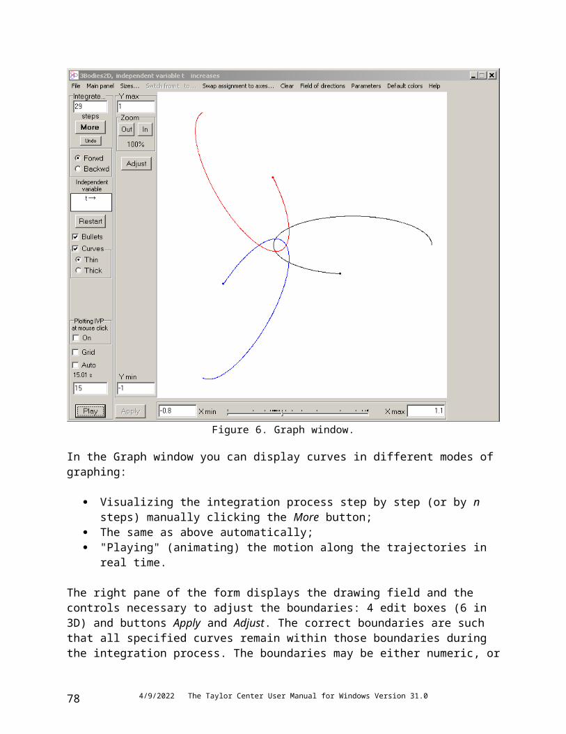
- Only a finite number of Taylor coefficients (30 by default) are available, and - The length of the numeric representation in the PC (64 bit mantissa, 15 bit exponent) is fixed

so that an overflow or a catastrophic subtraction error may happen.

The situation becomes particularly confusing when the convergence radius r of the solution happened to be infinite (meaning the solution is an entire function). For an entire function the step h in theory may be arbitrary big. However for any expansion which is infinite (i.e. not a polynomial) there exists such a big step h, that the Taylor terms at the beginning of the expansion violently grow and exceed any limitation of the computer float point format. This circumstance alone indicates that the usable step size may have nothing to do with the (infinite) convergence radius.

For non-polynomial solutions the program typically generates a finite rh (whether the function is entire or not), for example, x=et or u=cos t. However sometimes (see examples below) the algorithm may yield rh near machine infinity (if rh was not limited by the parameter Radius limit). By default, the Radius limit is set to a particular value (10, typical for a "macro" world). Yet depending on the scale and physical units of actual problems, it may require adjustments. For experiments with an "infinite" radius it must be set to the value near 104932 (the machine infinity).

For a system of ODEs comprised of only one trivial equation t'=1, or of a polynomial significantly below degree 30, the algorithm would yield rh near the machine infinity.

The generated rh is used as the first guess for the step h=0.5×rh. If this step size does not provide the required accuracy, the algorithm enters into a loop of step splitting. In order to asses how well the algorithm for rh works in cooperation with the coefficient k in the formula h=krh , you have to observe how many acts of splitting happens during integration of a particular problem. (Ideally we want no additional step splitting).

For solutions such as x=et or u=cos t (both entire functions) the program yields rh <10 at t=0. Try the respective ODEs: x'=x, or

u'=-vv'= u.

With the relative error tolerance 10-19 the generated rh allows integration without step splitting (with the default order 30 and k=0.5). Now make the relative tolerance smaller, say 10-25 (meaning the ultimate accuracy), and watch that step splitting does happen (the other conditions being the same).

So we see that useable h and rh dramatically differ from the infinite convergence radius. This difference is even more noticeable for a slightly modified ODE, say x'=-1000x, having the solution x=e-1000 t : also an entire function. For it the program generates rh as small as rh = 0.0052 . Here too splitting does happen (2-3 times) if the ultimate accuracy was specified. And again, by setting k=0.05 you can make splitting unnecessary.


In the cases of infinite convergence radius considered above the algorithm does generate practically usable heuristic radius rh << r = . Yet here is the case when the algorithm fails. Consider the problem5 (file y7x5_in_t.ode):

x' = -y7 xt=0=1y' = x5 yt=0=0

whose integral is known: x6/6 + y8/8 = 1/6 . Set the order of differentiation to 100 and the radius limit – "unlimited", i.e. 104932 . Now compile it and observe that rh = 5.198×10350: not usable. Looking into the debugging page you see that the expansion is sparse (filled with many zeros):

x[n] = 1, 0, 0, 0, 0, 0, 0, 0, -0.125, 0, 0, 0, 0, 0, 0, 0, 0.0303819, 0, 0, 0, 0, 0, 0, 0, -0.00950677, 0, 0, 0, 0, 0, 0, 0, 0.00326992, 0, 0, 0, 0, 0, 0, 0, -0.00118316, 0, 0, 0, 0, 0, 0, 0, 0.000441912, 0, 0, 0, 0, 0, 0, 0, -0.000168692, 0, 0, 0, 0, 0, 0, 0, 6.5428110-5, 0, 0, 0, 0, 0, 0, 0, -2.5686210-5, 0, 0, 0, 0, 0, 0, 0, 1.0180910-5, 0, 0, 0, 0, 0, 0, 0, -4.0665210-6, 0, 0, 0, 0, 0, 0, 0, 1.6346610-6, 0, 0, 0

Recompile it with the default radius limit of 10, so that rh=10, h=5, and try to integrate one step of this size (click the button More). This attempt fails with the message "Singularity reached". Now inspect the debugging page and observe that at t=5 values6 of x and its derivatives are enormously big:

x[n] = 2.063219946787781061, -2.6944510432, -5.908610677, 1.28605101049, -1.67951101420, 1.31601101791, -5.72877102161, 1.06878102532, 4.25382102779, -3.08625103150, 1.61219103521, -5.74207103891, 1.2498104262, -1.25552104632, -5.36123104880, ….

It appears that even step h=5 is too big for this particular series, causing violent growth of its terms quickly approaching the overflow (-5.36123104880) .

To remedy the problem, set the radius limit to 1. With this setting you will be able to integrate this ODEs along its entire period and even to maintain the ultimate accuracy.

5.2. Catastrophic subtraction error near singularities of ODEs Catastrophic cancellation error or catastrophic subtraction error is an error in the difference x=a-b when the approximate values a, b are so close, that only a few or none of significant digits of x are correct (due to the cancellation in the fixed length float point representation).

In the PC's real numbers type extended the mantissa contains 59 bits, which corresponds to 21 decimal digits. So in the following examples in theory

_ 0.999,999,999,999,999,999,999,997 0.999,999,999,999,999,999,999,995

0.000,000,000,000,000,000,000,002

5 The so called Generalized Harmonics (courtesy of Prof. Harley Flanders)6 In this and the following similar printouts only the first value is given with 15 significant digits, while the rest of them only with 6. In the actual program output the subscripted base 10 is displayed as letter e.


and

_ 800,000,000,000,000,000,000,001.0800,000,000,000,000,000,000,000.0 1.0

yet practically in both cases a computer would yield the machine zero 0.0 in the PC arithmetic, exemplifying the extreme case of a catastrophic subtraction error. Whether such a result is really catastrophic depends on the nature of the problem, and at which stage this happened.

The result is definitely catastrophic if it is the final step in the algorithm solving the problem – while you need many significant digits in this result. For example, if the goal is to compute a derivative of a non-linear differentiable function f(x) at x= x0 , f(x0)0 using the definition of derivative

f'(x0) = lim ( f(x0+h) – f(x0))/h

with some small enough value of h, we will clearly have a catastrophic subtraction error. Here is why. While h is finite and big enough, the result is coarse because f(x) is non-linear. Yet when h approaches zero, beginning with a small enough h the numerator becomes a machine zero so that the computed value of f'(x0) becomes the machine zero disregarding the value of h and the actual f'(x0).

The opposite case when the subtraction error is neither catastrophic not even affect the result is the average

(f(x0+h) + f(x0))/2

or an expression like this

1 + (f(x+h) – f(x))

with an arbitrary small h.

However the catastrophic subtraction error may emerge not only in differences occurring in the right hand sides, but also in expressions which become singular. Such expressions are either quotients when the denominator approaches zero, or elementary functions like ln x, or xa (with negative of non-integer a) when x approaches zero. To understand why, take a look at the formulas of differentiation for these expressions (Appendix 4). Those formulas are fractions whose denominator x approaches zero, causing the singularity in the ODEs and exceptions while evaluating these formulas.

Yet the solution at this point of the phase space still may be either singular or regular. In the latter case the numerator of the fraction must approach zero too. Those numerators in fact are differences, and it is because of them that a catastrophic subtraction error may emerge.


5.2.1. How to observe a singularity of the solution or of the ODESpeaking about a singularity of the solution itself, you hardly can bypass it unnoticed: some of the Taylor coefficient would behave violently.

However the situation is more complicate if the solution is regular but the ODEs are singular. How can you know then that you approach a singularity of those ODEs?7

Say, the solution is polynomial or holomorphic in a neighborhood of the initial point. As the solution is regular, the Cauchy formula (utilizing the well behaved Taylor coefficients of the solution) would yield a finite radius and no hints about singularity of the ODE. Then usually comes the effect of a catastrophic subtraction error caused by the singularity of the ODE (albeit not always). The following example illustrates such cases.

Compile a singular ODE

x'= 2x/t xt=- = 2 =10-10

whose solution is x=t2, and see the debugging page. Whichever small is specified, the computed Taylor serious reduces to a two terms which the PC happened to compute exactly in this case:

x[n] = 110-20, -210-10, 1, 0, 0, 0, 0, 0, 0, 0, 0, 0, 0, 0, 0, 0, 0, 0, 0, 0, 0, 0, 0, 0, 0, 0, 0, 0, 0, 0

You would see no indications of approaching the singularity of this ODE at t=0. You may specify the highest accuracy, integrate and even jump over t=0 (providing that t did not happen to hit exactly zero on the pass).

Now compile ODEs:

x = (et - 1)/t {auxiliary variable}t' = 1 (t = )

with various near zero values of and view the debugging page for values x[n]:

= -10-100

x[n] = 0, -110100, -110200, -110300, -110400, -110500, -110600, -110700, -110800, -110900, -1101000, -1101100, -1101200, -1101300, -1101400, -1101500, -1101600, -1101700, -1101800, -1101900, -1102000, -1102100, -1102200, -1102300, -1102400, -1102500, -1102600, -1102700, -1102800, 0

= -10-10

x[n] = 0.999999999798905, -1.01095, -1.510951010, -1.510951020, -1.510951030, -1.510951040, -1.510951050, -1.510951060, -1.510951070, -1.510951080, -1.510951090, -1.5109510100, -1.5109510110, -1.5109510120, -1.5109510130, -1.5109510140, -1.5109510150, -1.5109510160, -1.5109510170, -1.5109510180, -1.5109510190, -

7 Indeed, in this application we consider only such ODEs whose right hand sides are comprised of rational functions and a few traditional elementary functions, whose singularities are obvious for a mathematician. We are discussing here what will be the behavior of the program in such cases.


1.5109510200, -1.5109510210, -1.5109510220, -1.5109510230, -1.5109510240, -1.5109510250, -1.5109510260, -1.5109510270, 0

= -10-6

x[n] = 0.999999500000189, 0.5, 0.188935, 22268.6, 2.226851010, 2.226851016, 2.226851022, 2.226851028, 2.226851034, 2.226851040, 2.226851046, 2.226851052, 2.226851058, 2.226851064, 2.226851070, 2.226851076, 2.226851082, 2.226851088, 2.226851094, 2.2268510100, 2.2268510106, 2.2268510112, 2.2268510118, 2.2268510124, 2.2268510130, 2.2268510136, 2.2268510142, 2.2268510148, 2.2268510154, 0

= - 0.001

x[n] = 0.999500166625008, 0.499667, 0.166542, 0.0416334, 0.00833625, 0.0112477, 9.86019, 9859.99, 9.85999106, 9.85999109, 9.859991012, 9.859991015, 9.859991018, 9.859991021, 9.859991024, 9.859991027, 9.859991030, 9.859991033, 9.859991036, 9.859991039, 9.859991042, 9.859991045, 9.859991048, 9.859991051, 9.859991054, 9.859991057, 9.859991060, 9.859991063, 9.859991066, 0

Indeed, x(t) is holomorphic at t=0 and the exact values of x[n] near zero ought to be:

1, 1/2!, 1/3!, . . . , 1/n!, . . .

As you see, the computed Taylor coefficients violently diverge from the correct values in all these cases. The closer to zero, the earlier the Taylor coefficients diverge from the correct values, demonstrating an effect of catastrophic subtraction error.

You may replicate this behavior integrating the ODE satisfied by the same x(t)

x' = x + (1 - x)/t x|t = = (e - 1)/

for the same near zero values of = -0.001, -10-6, -10-10, -10-100.

Now set = -1 and try to integrate this ODE from t=-1 into positive values of t. If no error control was specified, you may even jump over the singularity of this ODE (if it did not happen that t=0 exactly alone the pass). However if you do set the error control, especially the ultimate accuracy, and try to jump over t=0, you will not be able to do that. While approaching zero, the program would split the step more and more – in response to the violent growth of the Taylor coefficients and rh approaching zero as a result.

This example does illustrate how the integration process stumbles approaching the singularity of ODEs while the solution itself is regular.

5.3. Unnoticed jumps over singularities: x' = -sqrt(x)As we have seen, sometimes it may happen that you jump over a singularity of ODE, especially if no error tolerance was specified. (Therefore after pilot integrations it is a good idea to set some error control). The following weird example illustrates a particularly puzzling behavior.

Open the program and enter an initial value problem (or load the file strange.ode)

t' = 1 {necessary in order to graph x(t)}


x' = -sqrt(x) x|t=0=1 (*)

The solution is a second degree polynomial x = ¼(t-2)2, a parabola so that the convergence radius is infinite. Yet the ODE8 has a singularity at the point t=2 where x reaches 0. (See more about such ODEs in the next section).

(a) Not modifying anything in the default settings, enter ODEs (*) or open the file strange.ode, compile it, then specify x(t) for graphing and look at the curve in the Graph window. Surprisingly, instead of a parabola you will see a wavy curve comprised of pieces of many parabolic arcs connected at points t=5, 10, 15, ….

Figure 9. At point (2, 0) the ODEs have a singularity, yet the program jumps over it from t=0 to t=5.

Here is what actually happens.

8 This ODE should be considered in complex space C, yet this package cannot deal with complex numbers. In fact, negative x causes an exception computing sqrt(x), and even x=0 causes an exception while evaluating derivatives of sqrt(x) being a point of branching singularity for Sqrt .The analytic function Sqrt has two branches +sqrt(t) and -sqrt(t). According to the theorem of existence and uniqueness, the solution exists and is unique in a neighborhood of any regular point for each of the branches. In the real space -sqrt(t) is negative, therefore ODE (*) may represent only decreasing part of the parabolic solution x = ¼(t-2)2, i.e. for t<2. To represent the increasing part of the solution for t>2 we need another ODE y' = +sqrt(y).


1) The solution (a polynomial) has an infinite convergence radius. The default heuristic radius limit is 10, so that the computed infinite value rh was cropped to 10 and h=0.5×rh

= 5. 2) From t=0 with step 5 program jumped over the singularity of the ODE (at the point t=2,

x=0), reaching the point t=5, x=9/4 : correct so far. 3) However an attempt to integrate the next step at t=5, x=9/4 for the same ODE (*) is

wrong, because on the right side of the singularity at t=2 of ODE (*) the parabola x = ¼(t-2)2 does not satisfy ODE (*) any more. Now this parabola x = ¼(t-2)2 satisfies the IVP for the positive branch of square root x' = +sqrt(x) (see footnote 5, page 48). An attempt to integrate a wrong ODE at point t=5, x=9/4 causes the next segment of the curve to dive down (instead of to go up). The similar situation repeats at the subsequent steps.

(b) This time set the radius limit to a value less than 2, say 1, then repeat compilation and graphing. Now the program, in attempt to integrate default 10 steps, ends up with the message "Singularity reached" making only 3 steps. Get into the Debugging page and observe, that both t and x reached 0. The formula of differentiation of sqrt includes division by x, and this obviously caused this exception. It happened at the fourth step with h=0.5, t=0.5×4=2.

Similarly try the radius limit 0.8, repeating compilation and graphing. Now the program also ends up with the message "Singularity reached" (after 4 steps). In the Debugging page observe, that while t reached 0, x happened to become a very small yet negative value x = -3.388131789017210-21 which caused an exception in attempt of computing the square root at the fifth step with h=0.4, t=0.4×5=2.

(c) Repeat the previous experiment with the radius limit 0.9 and h=0.45. Now the program "successfully" jumps over the singularity into positive values of t, yet goes on with the same wrong arcs of parabolas like in case (a) for the same reason: after bypassing this singularity the ODE must be changed.

(d) Now set the radius limit to such a value, that the h gets very close to 2. Let the radius limit be 3.999999 so that h= 1.9999995. Compile the problem and get into the Integration page. In it made just one step and look into the Debugging:

x[n] = 6.249997264520810-14, -2.510-7, 0.25, 0, -1.3552510-8, -0.0216841, -32526.1, -4.956361010, -7.744311016, -1.239091023, -2.023851029, -3.364321035, -5.677291041, -9.704771047, -1.677541054, -2.928071060, -5.154621066, -9.143041072, -1.632691079, -2.933111085, -5.297931091, -9.616411097, -1.7532910104, -3.2096910110, -5.8978110116, -1.0874410123, -2.0113910129, -3.7312810135, -6.9406310141, -1.2943110148

Recall: x(t) in fact is a square polynomial. Thus the violent behavior of these Taylor coefficients means that here is a catastrophic subtraction error in play again. Because of their violent growth these coefficients now generated rather a small value rh=110-5. Next step with this rh however ends with an exception caused by a small negative value of x.

(e) Finally repeat the experiment (d) – but now set the error control for x up to the ultimate accuracy (Middle step error control). The first step (being equal to the first step in case (d)) succeeds delivering the required tolerance without any splitting. However, unlike the case (d), in subsequent steps the error control now causes step splitting so that integration lasts longer,


visibly stumbling (as it should) at the point where x approaches 0. Yet several steps later it too ends with an exception cased by a small negative x. Even very small values of h cannot neutralize the violent growth of (catastrophically corrupted by the cancellation) Taylor coefficients, conducting to a negative x.

5.4. ODEs with "regular singularities" There exist special points in some ODEs which are singular for the right hand sides of the ODEs, yet the solution at such points may exist being regular and holomorphic. For example, the implicit ODE

tx' – 2x = 0 (x' = 2x/t) x|t=0 = 0

is singular at t=0, yet its general solution x=Ct2 does exist (being not unique because of the singularity), and the solution is holomorphic at t=0. Noticeably, this solution x=Ct2 satisfies also some regular ODE: for example, x' = 2Ct.

Similarly holomorphic solution x(t) = tet at t=0 satisfies both singular and regular ODEs:

tx' – tx – x = 0 (x' = x/t + x) (singular)

x" = 2x' – x (regular) .

However there exist holomorphic functions having such a special point, that it is impossible to find explicit rational non-singular system of ODEs satisfied by these functions. For example, such is the function x(t)=(et - 1)/t at t=0. This function in itself is entire, i.e. it has no singularities. However when we are looking for rational ODEs satisfied by x(t), whichever we find appears to be singular at t=0, for example

tx' – tx + x – 1 = 0 ( x' = x – (x-1)/t, ) x|t=0 = 1,

It was proven that no rational n-order ODE may be satisfied by functions x(t) and be regular (to have nonzero denominator) at t=0. As of now (01/30/18) it is not yet known whether x(t) may satisfy rational systems of ODEs regular at t=0..

So a special feature was added to the Taylor Center allowing it to deal with indefiniteness 0/0 in some singular ODEs satisfied by regular solutions. By no means does this feature attempt to address an arbitrary rational system of ODEs where the indefiniteness 0/0 occurs in the right hand sides. (For such systems another type of algorithm, developed by Pryce and Nedialkov, is required. It involves numerical solution of implicit equations by means of iterations).

This feature here is intended for teaching and research purposes only. It allows to integrate certain regular solutions through the points where the indefiniteness 0/0 occurs in the right hand sides. At that it is presumed, that the user knows where such special point of the solution is, and can provide the Taylor expansion for that particular special point.

As we will see below, many such functions and their expansions are really well known and considered in the Calculus.


5.4.1. How integration of singular ODEs is implementedIt is assumed that the given ODEs (or some of the auxiliary equations) have a known point of indefiniteness 0/0 in the right hand sides, say at t=t0. In all points except that special point these ODEs do allow to compute the Taylor expansion, yet at t=t0 they fail. For t=t0 another – some external – source of Taylor expansion is required. (In many cases such expansions may be found in textbooks).

The Taylor Center includes a sample program called SpecPoints.exe generating expansions for certain classical functions at the special points, and also several samples of files with such expansions, required for the Taylor Center in order to deal with special points.

The user can also create his/her own files of expansion in special points in any available programming system. It must be a file of numbers of type extended (10 byte float point format) containing the values

t0, a0, a1, a2, a3, ….. Here t0 is the special point - a value of the variable of integration (independent variable), at which an indefiniteness 0/0 occurs, and an are the Taylor coefficients of a function or of an expression w=u/v for which it happens that both u|t=t0=0 and v|t=t0=0. The program SpecPoints.exe by default creates expansions of order 100 (it may be changed). The Taylor Center loads these values up to the order set in the Taylor Center (default 30).

The file naming convention is such, that the special expansion file corresponding to problem MyProblem.ode is named MyProblem.sing being loaded automatically when the problem MyProblem.ode is opened. Also, after opening any problem MyProblem.ode the required special expansion file with any name may be loaded manually via menu item

Fill/Open special point …

When the proper special expansion file is loaded, then a singularity in the right hand side is allowed either in the initial point, or anywhere along the integration pass.

The evaluation algorithm of the Taylor method is modified such a way, that first it tries to evaluate all the derivatives of the right hand sides of the ODEs in the standard manner. If in the process of this evaluation it encounters an exception 0/0, the algorithm checks whether the point of evaluation is the special point t0, and if so, the algorithm utilizes the loaded special expansion. This way the algorithm evaluates the derivatives when being exactly at the special point, say if the initial value is that special point.

If the initial point is regular, and the special point therefore occurs on the integration pass, the following scenarios are possible.

1) The accuracy control of integration is not specified. Then the program sets integration steps in accordance with the current heuristic convergence radius only. In so doing, the incremented independent variable may rather jump over the special point (not creating any exceptions). If the current integration point by chance gets exactly into the special


point, then the processing happen like it was described above for the case when special point was the initial point.

2) The accuracy control of integration is specified. In such a case when integration approaches the special point, normally the step is repeatedly halved more and more, neither allowing to jump over the special point, nor to reach it. However with the special expansion loaded, the program computes the heuristic convergence radius r for this expansion. As soon as the integration reaches within the radius r of the special point, the program jumps into the special point avoiding the process of repeated halving of the step.

Further on we will discuss samples of various ODEs with singularities. In particular we will clarify how to distinguish situations when the loaded special expansion corresponds not directly to some function f, but rather to the derivative f' or f".

In all the following examples when file with ODEs xxxxxx.ode is loaded, the program automatically looks for and loads the respective special expansion file xxxxxx.sing . In all the examples the special point – the singularity of the ODE – occurs at t=0, which is also the initial point for these initial value problems. Normally the initial point must not be a singular point of the ODEs. However when the associated special expansion file xxxxxx.sing is available and loaded successfully, it makes possible the compilation (evaluation) of the derivatives at this "singular" initial point so that integration may go ahead to normal domain of regularity as usual.

All the expansions in the following sections are obtained via the program SpecPoints.exe. It allows to chose from the menu the function, to compute, to view and save the expansion, and to view the lines of the algorithm computing the respective expansion.

5.4.2. The functions defined directly via singular expressionsIn this section we consider the functions

(a) x(t) = t/(et - 1) (generating the Bernoulli numbers, file Bernoulli.ode);

(b) y(t) = (et - 1)/t (the inverse to x(t), file InvBernoulli.ode);

(c) z(t) = sin(t)/t (the file sin(t)Divt.ode)

(d) u(t) = ln(t+1)/t (the file ln(tplus1)divt.ode)

In each of the cases the function of interest appears in the Auxiliary variables section, and the ODE itself is trivial t'=1. The program encounters indefiniteness in an attempt to evaluate the respective auxiliary variables (x, y, z or u), and then it utilizes the special expansions for the respective functions. In this case these expansions correspond to the functions themselves (rather than to their 1st or 2nd derivatives).

For all the functions above the initial point may be chosen other than t=0, and then the integration process must successfully bypass the point t=0, where ODE has a singularity. The integration must successfully bypass the point t=0 also if the accuracy tolerance is set the highest.


Note: In situation when the ODEs are trivial (reduced to one ODE t'=1), and you wish to specify the accuracy for certain auxiliary variable, the table on the Integration page allows to specify accuracy only for the main variables. In order to estimate and control integration error for an auxiliary variable (say x) overcoming this limitation, introduce one more main variable, say y'=x, and then specify the accuracy tolerance for y.

5.4.3. The functions which may be defined only via singular ODEsUnlike the previous section, here the expressions for the functions of interest are not known. Instead these functions are defined via the ODEs which are singular at t=0.

(e) x'' = ( (p2 – t2)x – tx' )/t2 Bessel function Jp provided for p= 0, 1, 2 in files:

Bessel-0-2.ode for J0"Bessel-1-2.ode for J1"Bessel-2-2.ode for J2"

(f) x" = x/t in file tx2minusx.ode.

Here in both cases indefiniteness emerges in an attempt to evaluate the second derivative of the respective functions, and so are provided their expansions with the respective names loaded automatically. These functions are provided directly only at the initial point t=0 (i.e. at the point of special expansions). All other points may be reached via integration.

5.4.4. Function cos(sqrt(t))9

This function is particularly interesting for teaching purposes because of various reasons. In spite of singularity of sqrt(t) at t=0 on the complex plane, this function is an entire function.

Moreover, on the real axis despite that Sqrt(t) is imaginary for t<0, x(t)=cos(sqrt(t)) is real on the entire real axis. Yet we cannot use this expression directly because the program does not deal with complex values of sqrt(t) for t<0.

Instead we resort to ODEs for x(t) avoiding using of sqrt:

x" =- (x+2x')/(4t)

entered in the form

t=0 t'=1x=1 x' = x1 {x'}x1=-0.5 x1' = (-0.25)*(x + 2*x1)/t {x"}

(the respective file is cos(sqrt(t))-2.ode meaning the expansion is provided for x"). These ODEs may be integrated forward and backward demonstrating that this function indeed is not even, and it grows monotonously to infinity for t - .

9 This example is by courtesy of George Bergman


5.4.5. x' = -sqrt(x) revisited It is instructive to reconsider the weird ODE x' = -sqrt(x), x|t=0=1 which too exemplifies a singular ODE having an entire – moreover a polynomial – solution x = ¼(t-2)2 (the respective file is strange-1.ode providing the special expansion for x'). However, unlike the previous examples where the ODEs were regular everywhere except one point and real for real-valued variables, this ODE is not always real for real-valued x. Moreover, on a complex plane the point x=0 is a branching singular point in the ODE x' = -sqrt(x), so the solution x = ¼(t-2)2 cannot be continued beyond the point t=2, x=0 with the same negative branch of -sqrt. Now the integration with the program can reach the point t=0 (utilizing the special expansion). Yet an attempt of a next step generates the message Singularity reached, because the program attempts to increment negatively zero valued x and then to compute sqrt(x) i.e. square root of a negative value.

5.4.6. Graphing an isolated analytic element of any natureThis new feature of a special expansion allows also to explore (to graph) a single analytic element – a single expansion at one point for which no respective ODE is known (or perhaps does not exist in the class of elementary functions). Such is the example

x(t) = tn/nn

representing some entire function (which perhaps is not elementary, nor is known to satisfy any ODE). The program allows to draw the graph of this function as a segment corresponding to the above Taylor expansion up to the current order of approximation (default 30).

Load the corresponding file 1Divn^n.ode. It contains a trivial ODE t'=1 and an auxiliary variable u= 0/t to be graphed. At t=0 therefore due to the exception the program utilizes the special expansion above graphing it within the computed heuristic convergence radius. When you run this example with the default setting of the program, you will see the curve for t [0..10] and the straight line beyond it.

In order to watch the curve for t [-10..10], set the respective boundaries for OX, and not clearing the graph, click the control Forward switching it to Backward, click Restart and the button More for integration into the negative domain.

You may watch this curve in a wider segment. The default Radius limit crops the raidius with the value 10. Change it (in the main panel) say to 100 and reload the example. Now you will see its own radius a bit larger 13.6 so you will be able to redraw the curve in a wider range.

Finally, under File/Open special point and…/Assume convergence radius=Radius limit you can check up this mode, so that the convergence radius of the special element will be assumed the same as the radius limit (lastly set to 100). Now you will be able to redraw this segment with those wider boundaries (in which the fixed 30 degree polynomial will not accurately approach the function any more).

5.5. Conclusions1) As we have seen, potential points of catastrophic subtraction error are points of singularity of ODEs. However in this application singularities may occur only in rational and a few elementary


functions allowed to be used. As it is known in Automatic Differentiation, any system of ODEs whose right hand sides contain rational and elementary functions may be transformed to a wider system of ODEs whose right hand sides are polynomials. The polynomial system of ODEs does not have singularities in its phase space. Therefore, if an initial point of the source system is regular, integration from this point may proceed never reaching any singular point in the phase space of the respective polynomial ODEs10. With no singularities in the right hand side of such ODEs, the only remaining source of catastrophic subtraction error in polynomial systems is differences.

2) A situation of catastrophic subtraction error emerges only at isolated points: the points where a certain sum in a sub-expression approaches zero (in holomorphic functions zeros are always isolated). Therefore by a slight variation in integration step it is always possible to jump over points of catastrophic subtraction error (if they are not singular).

3) With the error control switched ON not only are you maintaining the required accuracy, but also occasional abnormality in the program behavior (the step splitting loop) warns you about approaching to a special point.

6. Integration in a complex planeAs currently designed, this software works with real valued ODEs along a real integration pass. However, with some simple preprocessing of the source ODEs, the software may be used for integration in the complex plane as well, and one of the samples (Demo/Spirals/Double spiral) exemplifies such a case. In it, the system

t' = 1x' = x² - y²+ 2xy - x -3.5y + 1 y' = -x² + y² + 2xy - y +3.5x - 1

in fact represents a complex function z() via its real (x) and imaginary (y) components:

z() = x() + iy(), = t + iu.

Complex function z() satisfies the ODE

z' = (1 - i)z² + (-1 + 3.5i)z + 1 – i

and the example in the Demo corresponds to integration along the path = t, s0 (the real axis). Therefore, this sample in the Demo exemplifies integration of a complex ODE along a particular path (in this case along the real axis). However, it is possible to specify also a complex path too.

A conversion of a complex system of ODEs into the respective (double sized) system in the real and imaginary parts is practically possible because we deal hear with rational right hand sides and a limited number of elementary functions for which the formulas expressing them via their

10 The solution however may have singularities, e.g. x(t)=1/(t-a) satisfying x'=-x2, or x(t)=tan t, x'= x2 +1. These singular solutions satisfy polynomial ODEs.


real and imaginary parts are readily available. Therefore, a general elementary complex system of ODEs

zk' = Pk(, z1, …, zn), k=1, 2, … , n, (independent variable = t + iu = rei)

converts into a system for real valued functions

xk' = Fk(t, u, x1, …, xn, y1, …, yn), k=1, 2, … , nyk' = Gk(t, u, x1, …, xn, y1, …, yn).

where points (t,u) belong to the arbitrary chosen integration path L, generally - a curve represented parametrically in real variables, say

t = f(s)u = g(s).

We assume that the given functions f(s) and g(s) are elementary functions admitted in this software so that we deal with the standard systems of ODEs in real valued functions with the independent variable s:

s' = 1xk' = Fk(f(s), g(s), x1, …, xn, y1, …, yn), k=1, 2, … , n (*)yk' = Gk(f(s), g(s), x1, …, xn, y1, …, yn)

yet representing the complex functions zk = xk + iyk along the integration path f(s) + ig(s). In particular, path L may be a straight line {s, b + ks} or {a + scos a, b + ssin a}, where a, b, a are constants.

The above is a setting for integration of one IVP along a one piece path: a curve or a straight line. However we can also integrate along a piecewise path passing through given points (a0,b0), (a1,b1), …, (aj,bj),… in a set of connected problems (as featured in this software). In particular we are interested in a piecewise linear path

s0 s1 … sj …(a0,b0) (a1,b1) … (aj,bj) …a0 a1 … aj …

whose pieces are defined parametrically as t = aj + (s - sj)cos aj, u = bj + (s - sj)sin aj . In a case of linear pieces, the software offers a better opportunity than bothering with a set of connected problem: It allows to change the angles aj of the path during the process of integration within only one IVP. To monitor this process the program offers a special window of a complex navigator of the integration path.

6.1 The complex navigator of the integration path(Applies in the next version).


7. The code for super fast integration As a side product, this software generates a code in 3-address instructions of an abstract processor implementing the n-order differentiation of the solution vector. The format of the instructions is

type TInstruction = recordty : (cc, cv, vc, vv); {flags for 1st and 2nd operands: (C)onstant or (V)ariable}op : char; {operation: +, -, *, /, ^, exp, ln, cos, …}i1, i2, i3 : word {addresses, i.e. indexes to elements of a dynamic array}end;

and they appear in the right pane of the Debugging page. In this program the abstract AD processor is implemented in Delphi-Pascal and stores the data in dynamic arrays. However thanks to the list of the instructions, all the sizes of the dimensions of these arrays become available after compilation of the ODEs. Since this moment it is possible to automatically generate a highly optimized code of the AD processor in Assembler relying on the sizes known during the generation (or compile) time (rather than during the run time). Running such an assembler code may speed up the integration tens times (when the speed is at issue in huge time critical problems).

8. Other tasksAs by-products of this system, a couple of other tasks may be solved.

8.1. Implicit functions

This package also allows “integration” of functions defined non-differentially. Let a function y(x) be defined via an implicit equation F(x,y) = 0 with the elementary function F. Then it is possible to obtain ODEs defining this function.

As function F(x,y) is elementary in both variables, we have to produce ODEs defining its partial derivatives Fx and Fy : both with rational right hand sides. (Obtaining Fx and Fy requires manual symbolic differentiation). Then, the differential equation for y(x) is well known from the Calculus:

y' = - Fx/Fy

Details how to obtain these ODEs and the initial values for them are discussed in Appendix 2.

8.2. Computing zeros (roots) of any functionsIf a function u1(t) is elementary, its zeros may be obtain by the method discussed in Section 4. The fact that it is elementary means that we can produce an initial value problem with rational right hand sides defining it, thus to exactly follow the section 4.1.

The method of finding zeros described in 4.2 is applicable not only to the solutions of ODEs but also to other holomorphic functions defined non-differentially through an implicit equation F(x,y) = 0 with the elementary function F (see Section 6.1).


Say, we want to find zeros of a polynomial t5 – p2t – p = 0, where p is a numeric parameter. Let x(t) = t5 – p2t – p, and t0 is guess value so that x(t0) = x0 . A function inverse to x(t) is an algebraic function t(x) which cannot be expressed via rational functions and radicals. However, it is a solution of an initial value problem:

tx' = 1/(5t4 – p2), t|x=x0 = t0 .

This problem should be integrated from x = x0 to x = 0, which would deliver one of the zeros.

8.3. Graphing functions specified parametricallyYou can study and graph such functions presenting them as a trivial Initial Value Problem. Suppose, given are equations

x = f(t), y = g(t) for t t0

where functions f and g are expressions allowed in the right hand sides of ODEs. Enter them into the Auxiliary variables box, adding the trivial ODE:

x = f(t)y = g(t)

t = t0 t' = 1

(See and Open file Mobius.ode as an example). Then you should Compile it. Note, that if the selector of the method for the convergence radius were in the position "Main variables" only, the radius of convergence for this trivial ODE would be infinite (by default it is limited by 10, but this limitation may be changed in Manu/Parameters). However the functions x = f(t), y = g(t) would generally have rather a finite convergence radius. Therefore it makes sense to switch the method to include also the auxiliary variables in elaboration of the radius.

After that, select the curves to graph in the Graph setting page, say {x(t), y(t)}, and go to the Graph window. Again, you have to specify there the reasonable boundaries, and to integrate with the More button as usual.

8.4. A binary/hexadecimal/decimal converter

There is also a converter for the internal binary values to their decimal or hexadecimal display. The internal binary values are in the float point type extended having 64-bit mantissa. It may be helpful for precision numeric experiments to see and modify the binary values down to one bit. With that in mind, the Integration setting page and Debugging page offer the following service. The numbers displayed in the column of values in the Debugging page, as well as the initial and current values in the integration page table, are normally displayed in their approximate decimal format. When you double click at any of those cells, the program opens the window where this selected value is already displayed with all exact hexadecimal (and decimal) digits (ignoring the sign). You can modify the hexadecimal representation, say change the last bit, obtain the


corresponding decimal representation, and to enter it as a new initial value (in the Integration page).

9. Merging with other elementary functionsThe operations and functions allowed in the right hand sides of the equations in this package (Table 1) are enough for the majority of applications. Yet what to do if the required elementary function is not in the list?

Although this version of the Taylor center doesn't do that automatically, it's still possible to manually merge the equations defining the functions not available in the limited list of this package – see Appendix 3 for more details.

Suppose, your source system is

uk' = fk(u1, … um); uk|t = t0 = ck , k = 1,2,…, m ,

or

u1' = f1(u1, … um); u1 = c1 (for t = t0). . . . . . . . . . .um' = fm(u1, … um); um = cm

requiring an unavailable elementary function x1(u1) in the right hand sides, say sinh (u1) which is not in the list of predefined functions in the Taylor Center. Then there must exist an initial value problem defining x1(u1), found in Math textbooks. In this case for the hyperbolic sine sinh it is

sinh' = cosh sinh|u1=0 = 0 cosh' = sinh cosh|u1=0 = 1

We introduce new variables sinhu1 = sinh (u1) and coshu1 = cosh (u1) for which the following equations take place:

sinhu1' = Dtsinhu1 = Dusinhu1*u1' = cosh*f1(u1, … um)coshu1' = Dtcoshu1 = Ducoshu1*u1' = sinh*f1(u1, … um)

Thus, we have an initial value problem for a larger system of ODEs

sinhu1' = cosh*f1(u1, … um) sinhu1 = sin(c1) (for t = t0)coshu1' = sinh*f1(u1, … um) coshu1 = cos(c1)u1' = f1(u1, … um) u1 = c1. . . . . . . . . . .um' = fm(u1, … um) um = cm

equivalent to the source problem, but without the function sinh in the right hand sides.

In the special case, if we need this function sinh as a function of an independent variable t only (rather than of the dependent u1), the larger system would look simpler:


sinh' = cosh sinh = 0 (for t = t0)cosh' = sinh cosh = 1u1' = f1(u1, … um) u1 = c1 . . . . . . . . . . .um' = fm(u1, … um) um = cm

Given the equations defining an elementary (vector-) function, say the function u1 (together with co-components u2,…,um)

t' = 1 t = t0u1' = f1(u1, … um); u1 = c1 (for t = t0). . . . . . . . . . .um' = fm(u1, … um); um = cm ,

we can obtain a system, defining the inverse to u1(t): let's name it T(u1).

This system is:

DuT = 1/ f1(u1, … um) T = t0Duu1 = 1 (for u1 = c1)Duu2 = f2(u1, … um) / f1(u1, … um) u2 = c2 . . . . . . . . . . .Duum = fm(u1, … um) / f1(u1, … um) um = cm.

Assuming, that now the dash ' means differentiation by u1, the system would look

T' = 1/ f1(u1, … um) T = t0 .u1' = 1 u1 = c1u2' = f2(u1, … um)/ f1(u1, … um) u2 = c2 . . . . . . . .um' = fm(u1, … um)/ f1(u1, … um) um = cm ,

For example, given the definition of the exponent

exp' = exp exp = 1t'= 1 t = 0

we obtain the definition of the logarithm

exp' = 1 exp = 1ln' = 1/exp ln = 0

After renaming the independent variable exp to the usual notation t, we come to a well known system

t' = 1 t = 1ln' = 1/t ln = 0


Another example: given the definition of tan(t),

t'= 1 t = 0tan' = 1 + tan2 tan = 0

let's obtain it for the arctan:

arctan' = 1 / (1 + tan2) arctan = 0tan' = 1 tan = 0

or in usual notation: arctan' = 1 / (1+ t2) arctan = 0t' = 1 t = 0


10. ReferencesThe list of recent publications by Alexander Gofen

on the modern Taylor method, elementary functions, the unifying view

1. The Taylor Center Demo for PCs.http://TaylorCenter.org/gofen/TaylorMethod.htm

2. Interactive Environment for the Taylor Integration (in 3D Stereo). In: Hamid R. Arabnia et al., (Eds), Proceedings of the 2005 International Conference on Scientific Computing (CSC 05), pp. 67-73, Las Vegas, Nevada, CSREA Press.

3. Visual Environment for the Taylor integration in 3D Stereo. In: Proceedings DMS 2007, the 13th Intern. Conf. on Distributed Multimedia Systems, pp. 251-255

4. Unremovable "removable" singularities. Complex Variables and Elliptic Equations, Vol. 53, No. 7, July 2008, pp. 633-642

5. The ordinary differential equations and automatic differentiation unified. Complex Variables and Elliptic Equations, Vol. 54, No. 9, September 2009, pp. 825-854

6. Using the Taylor Center to Teach ODEs. CODEE Journal, 2012.


http://www.codee.org/library/articles/using-the-taylor-center-to-teach-odes/using-the-taylor-center.pdf

http://TaylorCenter.org/gofen/UnifiedView.pdf

http://TaylorCenter.org/gofen/UnremovSingularity.pdf

http://TaylorCenter.org/gofen/VisualTaylor.pdf

http://TaylorCenter.org/gofen/TaylorCenterPC.pdf

http://www.taylorcenter.org/gofen/TaylorMethod.htm

Appendix 1: Summary of important parameters and controls

Main window: GeneralOrder of differentiation (default 30) Main menu/Parameters

Convergence radius upper limit Main menu/Parameters

Direction of the integration Forward/Backward radio buttons

Editing equations, initial values, parameters, method for computing the convergence radius, opening the Polynomial Designer

Equations setting page

Specifying method of error control and error tolerances, number of elements to be stored, terminal value (if any), blind integration controls (if compiled successfully)

Integration setting page

Specifying trajectories for 2D/3D graphing (if compiled successfully)

Graph setting page

Inspecting values of the variables and elements (if compiled successfully)

Debugging page

Opening graph window (if compiled successfully) Main menu/Graph

Main window: Equations setting pageSpecifying degrees or radians (in expressions for constants or initial values)

Degrees/Radians radio buttons

Specifying how large set of variables to use for obtaining heuristic convergence radius

Radio buttons in box "Variables used for convergence radius"


Main window: Integration setting pageQuotient q=h/R (default 0.5) Corresponding edit control

Back step, Middle step or No error check Corresponding radio buttons

To continue or not integration if after maximum number of step splits the error tolerance failed

Go despite error check box

Absolute and relative error tolerances Corresponding columns in the table

To specify the Result array of elements anew, and for which set of variables

Specify the number of elements for the Result array. Check box if your wish the array to be circular. Check the boxes for the respective kinds of variables.

How many elements to store Edit control in Results array

Make Result array Circular (not appendable) Check box Circular

To append non-circular array Button Append

Restart blind integration from initial values Restart button

Specifying how many steps n must be performedon More button click

Edit control in Integrate panel

Integrate n steps more Button More

Specifying terminal value (if any) Edit control To …

Applying terminal value Check button Terminating condition

Making current values new initial values Button

Placing current values into clipboard on filefor exporting into another initial value problem

Button

Making clipboard values new initial values Button

Copy the entire table into the clipboard Button Copy to clipboard

Switching to the connected problems Button Switch


Main window: Graph setting pageSpecifying curves to graph Table "Select functions to

graph"

To generate automatically all curves corresponding to variables having format x, y, x1, y1, x2, y2, … or x1, y1, z1, x2, y2, z2,… - in 3D

Button {x1, y1}…

Generating the curves data according to the selection and switching to the Graph window restarting the integration.

Button Apply

Switching back to the Graph window (without restarting the integration) Button Graph

An attempt to applying previous boundaries and curves to changed equations Button Previous

Specifying 2D or 3D graphing Corresponding radio buttons

Specifying Red/Blue or Blue/Red glasses for 3D graphing Click onto the glass icon

Specifying a field of directions for one of curves Select one curve in the list

Graph windowMin/Max values along X , Y (and Z) axes(the 3D cage sizes)

Corresponding edit controls,then Apply button

Quick specification of the boundaries for a few standard areas

Menu item Size

Swapping the assignment of the curves to the coordinate axes:X ↔ Y, X ↔ Z, or Y ↔ Z.

Menu item Swap axes

Adjusting the boundaries to accommodate the curves,whose elements are stored in Results array (Integration setting page, Main panel)

Adjust button

Increasing the boundaries proportionally 1.25 times (zooming out)

Button "Zoom Out"

Decreasing the boundaries proportionally 1.25 times(zooming in)

Button "Zoom In"

Restart integration from initial values Restart button

Specifying how many steps n must be performed on More button click

The edit control in Steps panel

Integrate n steps more Button More (Space bar)


"Playing" the motion whose elements were stored Button Play

Specifying the playing time (sec) The edit control above the Play button

Perform auto integration in a given time intervals (sec)without clicking button More (or Space bar)

Check box Auto

Displaying trajectories as 1 pixel thin curves with no bullets

Check box Lines, item Thin

Displaying trajectories as thick curves Check box Linesitem Thick

Displaying bullets and trajectories as1 pixel thin traces of bullets

Check box Linesitem Bullets

Displaying m×n grid on graph field Check box Grid

To activate the mouse click action drawing a new IVP for theinitial values under the mouse click

Check button Mouse action

Drawing a field of directions for one of curves Menu item Field of directions

Rotation of non-planar 3D curves Slide controls and , orthe values in the table undermenu Paramters/3D scene

To control whether the rotation center at the center of the cage is anchored or movable during turns

The nameless check box between the and handles: The center is anchoredif the check box is checked

Axonometric view of 3D curves Axonometric radio button

Display the right or the left of the axonometric stereo pair The respective radio buttons

Switch skew resolution On Skew check box

3D stereo anaglyph view Stereo radio button

Visualize 3D cage of the parallelepiped Cage check box

Specifying parameters of stereo viewing The table under menuParameters/3D scene

Specifying parameters of the Field of directions

The table under menuParameters/Field of directions

Specifying bullet size (and thickness of curves in the Thick mode )

Menu item Parameters/Line width


Specifying curve density as distancebetween dots on curve in pixels (0.25 to 5 – dotted line)

Menu item Parameters/Curve density


Appendix 2. The modern Taylor method basics

The classical Taylor method (18 century) is based on the idea that an Initial Value Problem for the explicit system of ODEs actually defines the rule for computing all the higher order derivatives of the solution, and therefore allows obtaining the Taylor expansion for them. All the higher order derivatives may be computed by applying the differential operator Dn=(d/dt)n to both parts. As such, the Taylor method had not been considered as a numerical method for computers at least for two reasons: applying the formulas for n-th derivative to complicate expressions (superposition of several functions in the right hand sides) is both challenging and computationally wasteful (due to the exponentially growing volume of calculations in general case).

On the contrary, the Modern Taylor Method (the 60s of the 20th century) capitalizes on the fact that whichever complicated the right hand sides are, they may be reduced to a sequence of simple formulas involving one of the four arithmetical operations or several well known simple functions over no more than two variables. For them the rule of computing n-th derivative requires only O(n2) operations and it is easily programmable. Unlike its classical counterpart, not only does the Modern Taylor Method become viable and competitive for computer implementation; it also demonstrates several unique features.

In the Modern Taylor Method (and everywhere in this package) the concept of n-th derivative means the so called normalized derivative, which by definition is

u[n] = u(n)/n!

so that the Taylor expansion looks like this:

u(t) = u[k](t - t0)k

Exactly these Taylor coefficients u[k] are displayed on the Debugging page after a successful compilation. The expansions for the solution in points of integration are stored in a dynamic array Results, which may be saved (or loaded) from files, or used in other applications.

The order of differentiation (by default 30) is a fundamental parameter, and it may be changed before compilation of any problem. It affects the speed, the required memory and the strategy of integration on the given segment. If there is no special reason (like studying the growth of Taylor coefficients at certain point), it is not recommended to essentially increase it.

If number of the differential equations (or that of the main variables) is m, number of all variables is M (including the main variables), and the number of terms in the Taylor series is MaxOrder, the integration process requires M*MaxOrder*10 bytes. The array Results for storing P analytical elements (polynomials) requires m*P*MaxOrder*10 bytes.

In general, finding the optimal strategy to cover the given segment of integration with the minimal volume of computation requires additional study and experiments. In particular, it requires certain methods to estimate the convergence radius at each point. Then, the strategy should suggest how to select the right order of differentiation and the step to achieve the


required accuracy at each step of integration.

R. Moore (1960) suggested a heuristic rule of thumb (based on very simplistic assumptions): the optimal order of differentiation equals to the decimal number of digits in a mantissa of the float point representation at the given computer (for the type extended it is 20), while the integration step ratio must be approximately 0.1.

By default, step h is set to half the heuristic radius of convergence R. The algorithm to find it is based on the formula of Cauchy-Hadamard

___R-1 = lim |an|1/n

n

where Taylor coefficients an are obtained for each unknown function in the source ODEs. Each component of the solution may have its own radius, thus the procedure selects the minimal among them, which should be considered as a convergence radius for the whole system. Although the formula is exact, the result is heuristic because the formula is applied to only a finite number of terms, with simplified assumptions for obtaining the upper limit, and with a coarse (but very fast) method of raising to the fraction powers (using just the exponents in the float point representation).

1. Something to compare with Just to satisfy the curiosity of some users, here are the formulas for computing n-th order derivatives of a simple product vs. the formula for a superposition of functions as in a general ODE uk' = fk(u1, … um).

The Leibnitz formula for a product n

(uv)[n] =u[i]v[n-i]

i=0

requires only O(N2) operations

The multivariate Faa di Bruno formula for a superposition (in the normalized derivatives) is m m n uk

[n+1] = uini fk(u1, … um)ui[j] nij

i=1 i=1 j=1

where the summation is made over all indexes nij, ni which are the solutions of the equations m n n

jnij= N, ni= nij i=1 j=1 j=1

The required number of operation for it grows exponentially with n. That is what makes the difference between the Classical and Modern Taylor Methods.


Appendix 3: The basic results on elementary functions

The essential property of the elementary functions is unlimited expandability of their list by means of the two major operations: (1) obtaining a superposition of given elementary functions, and (2) obtaining an inverse to a given function. Then, as soon as we know that certain functions are elementary so that we can produce the rational ODEs defining their elementarity, we may use these functions in the expressions in the right hand sides of other ODEs. The following Main Theorem demonstrates the way and proves it.

1. Reduction to the Rational ODEs: the Main TheoremSuppose, our source system and IVP are

uk' = fk(u1, … um); uk|t = t0 = ak , k = 1,2,…, m , (1)

whose right hand sides fk are elementary functions (but not necessarily rational). These elementary functions may be such as say hyperbolic arctan, but also any sophisticated user defined elementary functions, i.e. functions defined as solutions of initial value problem of some other ODEs such that their right hand sides are rational.

The following Main theorem delivers a general constructive method of reducing any elementary system of ODEs to the rational format (which, of course, is always allowed in Taylor solvers).

The Main Theorem: an initial value problem (1) with elementary right hand sides may be widened to a larger initial value problem with rational right hand sides.

Proof. We are going to constructively obtain this larger system of ODEs as well the initial values for it.

As the vector-function {fk} is elementary by all its variables, there exist m systems (j = 1,2,…,m) of ODEs with respect to u1, u2, …, um

dfi/duj = Rij(f1,…fm,…,fM), fi|uj=0 = cij, , i = 1,2,…,M, M>m (2)

with rational right hand sides Rij and the corresponding initial values, defining the vector-function {fk}. Let's introduce new variables

vi = fi(u1, … um); vi|t = t0 = bi = fi(a1, … am); i = 1,2,…,M

satisfying the differential equations m m m

vi' = [fi(u1, … um)]' = (dfi/duj)uj' = Rij(f1,…fm,…,fM)vj = Rij(v1,…vm,…,vM)vj .j=1 j=1 j=1

Together with equations (1), it presents a closed system of ODEs:

uk' = vk , uk|t = t0 = ak , k = 1,2,…, m , m


vi' = Rij(v1,…vm,…,vM)vj , vi|t = t0 = bi = fi(a1, … am), i = 1,2,…,M.j=1

Thus, the source system is reduced to ODEs with the rational right hand sides. It remains to show the way how to obtain all required initial values.

The numeric values bi = fi(a1, … am) may be obtained either directly, if the corresponding procedures for fi are available in the Taylor Center, or otherwise via integration of each of the m additional initial value problems (3) by…

By u1: from ci1 to a1 , i.e. from vi = fi(ci1 , ci2 ,…, cim) to vi = fi(a1, ci2 ,…, cim), i= 1,2,…,M;

By u2: from ci2 to a2 , i.e. from vi = fi(a1 , ci2 ,…, cim) to vi = fi(a1, a2 ,…, cim), i= 1,2,…,M;

. . . . . . . . . . . . . . . . . (3)

By um: from cim to am , i.e. from vi = fi(a1 , a2 ,…, cim) to vi = fi(a1, a2 ,…, am), i= 1,2,…,M.

So, the required initial values vi = fi(a1, a2 ,…, am), i = 1,2,…,M are obtainable even if there is no preprogrammed procedure computing functions fi. That concludes the theorem, giving a constructive way of reducing an initial value problem with elementary (but non-rational ODEs) to the rational format.

Note: Practically it does matter whether the elementary functions in the right hand sides of the source system are system-supplied, or on the contrary, they are user-defined by means of other initial value problems. In the former case the required initial values (3) may be simply computed via the system-supplied procedures like sin, cos, tan, arctan et cetera in any necessary points, while in the latter case we do need to integrate the auxiliary initial value problems (3) in order to obtain all those vi = fi(a1, a2 ,…, am), i = 1,2,…,M .

Example. First we are going to consider an example which doesn't have any meaning in applications, but it illustrates the essence of the transformations applied in the theorem. In particular, it uses a rather exotic elementary vector-function non-reducible to the rational functions, to radicals or any other “traditional” elementary functions of one or several variables. Let us consider equations

u' = X(u, v), u|t=0 = 1 (4)v' = u2 v|t=0 = 1

where function X(y,z) is elementary being the inverse (by x) to a polynomial function:

P(x,y,z) = x5 – y2x – y – z = 0; z|x=1; y=0 = 1 .

This X(y,z) exemplifies an algebraic function non-reducible to the rational functions and radicals of any degree. Nevertheless, this function is elementary (as the inverse to a polynomial). The differential equations demonstrating its elementariness and defining X(y,z) are obtainable via differentiation of the equation P(X,y,z) = 0.

By y:


Xy' = (2Xy + 1)/(5X4 – y2); X|y=0; z=1 = 1; (z is a parameter). y' = 1

By z:

Xz'= 1/(5X4 – y2); X|z=1; y=0 = 1; (y is a parameter). z' = 1

To reduce the system (4) to the rational format, introduce a variable w = X(u,v) so that the first equations of (4) becomes u' = w. Now we need to obtain a differential equation for w:

w' = Xy'(u,v)u' + Xz'(u,v)v' =w(2wu + 1)/(5w4 – u2) + u2/(5w4 – u2) = [u' = X(u,v) = w; v' = u2 ]

= (2w2u + w + u2)/(5w4 – u2).

This closes the system (4), which is reduced now to the rational format

u' = w, v' = u2

w' = (2w2u + w + u2)/(5w4 – u2)

with the initial values

u|t=0 = 1 v|t=0 = 1w|t=0 = X(1,1) .

The value X(1,1) is not yet known, thus first the system (4) must be integrated from X(0,1) to X(1,1) by y.

On the contrary, the examples in the Chapter 6 are very practical and they show how to manually reduce a non-rational source system of ODEs (containing well known predefined elementary functions) to the rational format, usable in the Taylor Center (manual merging).

2. Transformation of an Implicit Equation to ODEsLet a function y(x) be defined via an implicit equation F(x,y) = 0 with the elementary function F. Then, it is possible to obtain ODEs defining y(x).

It is easier to start with a more general equation F(x,y) = c, so that y = y(x,c) and

F(x, y(x,c)) = c . (4)

Write down a differential equation for y as a function of x:

Fx + yx'Fy = 0, or yx' = - Fx/Fy , (6)


and then another one for y as a function of c:

Fx + yc'Fy = 1, or yc' =(1 - Fx)/Fy (7)

As the function F(x,y) is elementary in both variables, Fx and Fy must be expressible via rational functions of F (and probably others). Thus we can assume the right hand sides of the equations (6) and (7) being certain known rational functions. Now we have to obtain the right initial values.

Let start with arbitrary x0, y0, for which F(x0,y0) = c0 . Then, beginning with (6), we have an initial value problem yc' =(1 - Fx)/Fy , y|x=x0, c=c0 = y0 ,

to be integrated from c=c0 to c=0 . If we are successful, we obtain y1 = y|x=x0, c=0 such that

F(x0, y1) = 0 .

Now, with these values x0, y1 – solutions of the implicit equation F(x,y) = 0, we can finally write down the initial value problem

yx' = - Fx/Fy , y|x=x0, c=0 = y1

defining exactly that function y(x) we are looking for.


Appendix 4: AD formulas for major operations(all derivatives are normalized adsorbing the factorial)

1

Multiplication N

(uv)[N] = u[i]v[N-i]

i=0

Leibnitz formula: N additions, N+1 multiplications. Complexity 1 L

2 Square

N/2

(u2)[N] = 2 u[i]u[N-i] + (u[N/2])2 ; (even N) i=0

N/2

(u2)[N] = 2 u[i]u[N-i] ; (odd N) i=0

Complexity 0.5 L

3

Division

R = u/v

N-1

R[N] = (u[N] - R[i]v[N-i]) / v i=0

Complexity 1 L

4In particular, for

R' = u'v

N-1

R[N] = (1-i/N)v[i]u[N-i]

i=0

Requires N-1 additions, 2N multiplications. Complexity 1 E

5In particular, for

R' = u'/v

N-1

R[N] = (u[N] - (i/N)R[i]v[N-i]) / v i=1

Complexity 1 E

6Constant exponent aR = ua

N-1

R[N] = ((a(1-i/N) - (i/N))R[i]u[N-i]) / u i=0

Complexity 1 E

7Constant base eR = eu

N-1

R[N] = (1 - i/N)R[i]u[N-i]

i=0Complexity 1 E

8Constant base aR = au

N-1

R[N] = ln(a) (1 - i/N)R[i]u[N-i]

i=0Complexity 1 E

9Natural logarithmR=ln(u)

N-1

R[N] = (u[N] - (1-i/N)R[N-i]u[i]) / u i=1

Complexity 1 E


Differentiation of a quotient with indefiniteness 0/0

10

P = cos(u) P' = -Qu'

Q = sin(u) Q' = Pu'

N-1

P[N] = - (1-i/N)Q[i]u[N-i]

i=0

N-1

Q[N] = (1-i/N)P[i]u[N-i]

i=0

11P = tan(u) Q = P2+1

P' = (P2+1)u'=Qu'

See Square (item 2)

See item 4

12P=1 – u2

S= sqrt(P)R = arccos(u), R' =-u'/SQ = arcsin(u), R' = u'/S

See Square (item 2)See Sqrt (item 6)See item 5

13Division, v0R = u/vv0

N-1

R[N] = (u[N] - R[i]v[N-i]) / v i=0

14Division, v=0,but v'0 and R = u/v isHolomorphic at the point

N-1

R[N] = (u[N+1] - R[i]v[N+1-i]) / v' i=0

15Division, v[i]=0, i=0, . . . , p-1,but v[p]0 and R = u/v isHolomorphic at the point

N-1

R[N] = (u[N+p] - R[i]v[N+p-i]) / v[p]

i=0


Appendix 5: A Dynamic Link Library for vector-functions computed from their Taylor expansions

5.1. A sophisticated ODE solution as a library function The goal is to provide a stand alone function (for various programming languages under Windows) computing the vector-function of a solution of ODEs. It is presumed that first the solution is obtained with the Taylor Center as a set of Taylor expansions. Later the user is given an opportunity to compute the components of the solution without using the Taylor Center and without replication of the laborious integration process. Instead the stand alone DLL function implements the optimized (Horner algorithm) for computation of the desired vector function using the polynomial expansions obtained from the Taylor integration and saved in a binary file. The users in other programming languages (and in Delphi) will be able to utilize this function (just like other standard library functions) for their computational needs.

The Taylor Center saves a big binary file Results containing the Taylor expansions at nodes of an array, so that the DLL gives a user an access and utilizes this set of expansions in a form of a conventional function call delivering a high accuracy function value f(x) at any desired point in the domain covered by the expansions.

Note 1: It makes sense to use this function only when random access to f(x) is needed. If the goal is to obtain the tabulated values of this function at a regular grid, you should use the Save as Table menu item and save the regularly tabulated function as a binary file.

Note 2: Generally, the array Results may store the expansions obtained via integration in more than one independent variable. Even if the array Results contains expansions for integration in only one variable, say t, it still is possible that the direction of integration had been changed from Forward to Backward several times during the integration process. The limitation of this DLL is that it applies only to such an array Results which was obtained in integration for one independent variable only and without any reversals of the direction.

The declaration of the array Results is

Results : array[0..P-1, 0..VarNum-1, 0..MaxOrder-1] of extended;

Here P is a number of nodes where the Taylor expansions were obtained, VarNum – a number of the main variables in the system of ODEs plus possibly the Auxiliary variables, MaxOrder – the number of terms in the Taylor series (the highest order of differentiation plus 1), and the type extended is the 10-byte float point representation with 64-bit mantissa (Intel extended precision LONG DOUBLE). During the initialization stage the DLL automatically retrieves these dimensions from the file and loads all the expansions into the memory.

The user should know the name of the binary file (with extension *.elm) containing the array Results, say MyVectorFunction.elm, and the indexes of the variables of interest of the vector-function of the IVP. For example, if the vector-function was (x, y, t, u, v) so that VarNum=5, and if the user needs the components x(t), y(t), their indexes are 0, 1 (the indexes are counted from 0).


Note 3: This 32-bit Windows DLL applies only in the programming languages which implement the Intel extended precision LONG DOUBLE exactly as the 10 byte float point type. For that reason, for example, this DLL does not work with MS Visual Studio C++, where the LONG DOUBLE is reduced to 8 byte DOUBLE type.

5.2. How to use this DLLThe name of DLL is TCenterOutput.dll .

This DLL exports the following functions: Init, SetNearestNode, ClearNearestNode, OneFunction, TaylorExpansion, NumberOfNodes, NumberOfVars, Order, TaylorTerm,LowNode, HighNode, explained below. All formal parameters in the functions below are called by value.

function Init(FullPath : PChar) : boolean; stdcall;

Here FullPath (a null-terminated string) corresponds to the data file generated during integration, say MyVectorFunction.elm, containing the Taylor expansions of the vector function at some irregular grid of nodes. (The grid of nodes is irregular because every next node must be within the convergence radius proper to the previous node, and the distance between the nodes must guarantee the specified accuracy). Function Init returns the value True, if the initialization succeeds and the limitations of the Note 2 are not violated.

The Init procedure may fail with the following messages:

Failed to open file of elements – when the file is corrupted; No independent variable in the array – when the system of ODEs didn't include the trivial

ODE for the independent variable like t' = 1; The array contains integration in more than one variable; The array contains integration in reverse direction.

Further on in order to optimize the computation of the vector-function of its argument (say t) in your algorithm, first you have to obtain the nearest node to t with the procedure SetNearestNode, and then to obtain the components of the vector function at point t.

function SetNearestNode(t : extended) : integer; stdcall; {-1 if wrong}

Here t is an argument for the subsequent calls of components of the vector-function (say u(t) and v(t) ). The function sets the internal index of the nearest node (and also returns its value). If the argument t is within the covered domain, the returned index is non-negative, or -1 otherwise, meaning the failure of the operation. As the nodes in the irregular grid are monotonously growing, this function implements the binary search requiring no more than log2N operations in a grid of N nodes.

function OneFunction(n : integer) : extended; stdcall;


The function returns the n-th component of the vector-function computed at the point t specified in the last SetNearestNode call. For example, the statements

u := OneFunction(3); v := OneFunction(4);

delivers u(t) and v(t) in the vector-function (x, y, t, u, v) for the lastly set value of t.

function TaylorExpansion(n : integer) : Pextended; stdcall;

returns a pointer to a value of type TExpansion = array[0..Order-1] of extended pointing to the first element of the internal array Results[RecentNearestIndex, n, 0] of the Taylor expansion for the n-th component of the solution vector at the grid point RecentNearestIndex nearest to t in the last call SetNearestNode(t). You can use this pointer to access any element of type TExpansion. function TaylorTerm(Node, Variable, Term : integer) : extended; stdcall;

returns an element Results[Node, Variable, Term] of the above mentioned internal array, i.e. the Taylor coefficient of the number Term of the component of the vector function number Variable at the node number Node.

function LowNode : extended; stdcall;function HighNode : extended; stdcall;

return respectively the lowest and highest boundaries for the argument t.

function NumberOfNodes : integer; stdcall;function NumberOfVars : integer; stdcall;function Order : integer; stdcall;

return the respective numbers characterizing the array of expansions.

procedure ClearNearestNode; stdcall;

clears the recent index of the nearest node.


Appendix 6: Setting Parameters for 3D Stereo

Viewing 3D stereo images requires that your vision in both eyes be approximately of the same acuity. You should wear the anaglyph (red/blue) glasses (in addition to your regular ones) and select the right type (red/blue, right/left) on the Graph setting page. The preinstalled setting assumes that you watch at the screen about 30 cm width from a distance about 50 cm, fixating at the point near the center of the screen (about 45 cm from your eyes) while the front of the 3D scene is about 25 cm from your eyes. This setting works OK also for computer controlled wall projectors (assuming the sizes increase more or less proportionally).

The whole setting is shown below: R and L are the right and left eyes respectively, CD is a distance to the front of the 3D scene, CF is a distance to the convergence point of your eyes, and CS is a distance to the screen.

The geometrical principle of the stereo vision is in that the human brain receives a pair of images – a stereo pair of projections, whose optical axes cross at a certain fixation point F. The brain establishes congruency between the corresponding points of images in the stereo pair. In doing that, it can even ignore the different colors of the corresponding points, like in the case of using anaglyphic glasses. Then, it analyzes the differences in directions to the corresponding points of the stereo pair – the so called disparities. These disparities, plus the expectations and knowledge about the real world makes it possible for the brain to “restore” the real 3D scene and to create a vivid impression as though the 3D scene is real.

The disparity of the fixation point F is 0, while for points in front of the fixation and those behind of it the disparities are of the opposite signs. The brain can “fuse” stereo pair well only if the absolute values of disparities do not exceed a couple of degrees. Thus, do not “place” the front face of the 3D scene too close to your eyes.

By default the XOY plane is parallel to the screen (the axis OX is horizontal, OY – vertical), while the axis OZ is perpendicular to the screen and directed to the viewer. You can turn the


R

L

F

3D scene

SC D

114

coordinate system specifying two angles: the rotation angle of axes OX and OY in the XOY plane, and the rotation of the axis OZ. These values become valid as soon as you close this window for setting the 3D parameters. If the integration was stored in array Results, the curves will be automatically re-drawn with respect to the turned coordinates. If the array was not stored, the screen will be cleaned, and the curves would not reappear.

1 0 0Ax = 0 cos α sin α

0 -sin α cos α

cos β 0 -sin βAy = 0 1 0

sin β 0 cos β

cos γ sin γ 0Az = - sin γ cos γ 0

0 0 1

cos β cos γ -cos α sin γ + sin α sin β cos γ sin α sin γ + cos α sin β cos γ cos β sin γ cos α cos γ + sin α sin β sin γ -sin α cos γ + cos α sin β sin γ -sin β sin α cos β cos α cos β


Appendix 7: Examples of tube plot and skew resolution Skew resolution algorithm applies only to the Thick line drawing mode (as this effect is hardly visible for 1 dot width curves set by default). For illustration purposes we are going to use images obtained for the example Demo/4 bodies/Torus representing a motion of two coupled pairs whose trajectory looks like an outline of Torus (though flattened at the top and bottom).

Here is the trajectory plotted as thin curve.


Now – the same trajectory plotted in the mode of Thick curves, yet without the skew resolution. The stereo view helps to detect which piece is over which, however the illusory intersection of the pieces is confusing.


And now the same trajectories of the slightly turned sample are plotted with the Tube Plot On


Appendix 8: Formal Definition of a Stiffness in ODEs and Dealing with It

In this part we speak about Initial Value Problems (IVPs) for systems of holomorphic Ordinary Differential Equations (ODEs) on an integration path not containing singularities. The goal is to introduce the definition of stiffness which conforms to this concept widely used intuitively in the recent decades.

In our view, this concept makes sense only for combination of an IVP and the integration segment for which the problem must be solved.

Definition 1. We call an Initial-to-Terminal Value problem (ITVP) an IVP for which also the terminal value is specified, so that the problem must be integrated from an initial value t=a to a terminal value t=b over a segment [a, b].

Our definition of stiffness thus will apply to ITVPs (rather than IVPs). Moreover, this definition will refer to and depend on a specific numeric method and its parameters used for integration of the given ITVP (rather than being an intrinsic property of the ODEs and ITVP alone).

Definition 2. Given the specific numeric method and its parameters, we call the Stiffness of an ITVP the number of steps required to integrate it from a to b under the parameters and requirements of the method.

The very language of this definition belongs to the applied rather than pure mathematics.

Remark 1. In terms of pure mathematics (ignoring technicalities of the computer implementation and the volume of computation) any ITVP may be integrated in one step using its Taylor expansion at the initial point.

Proof. If all components of the solution are entire functions so that their Taylor expansions have an infinite convergence radius, the Taylor expansions converge to the solution with any length of the segment [a, b]. Otherwise, if the Taylor expansions have a finite radius of convergence r < |b – a|, apply a proper summation method for this Taylor expansion. Such a summation of the Taylor expansion converges in a star-like infinite area (rather than merely in a disk) so that any terminal point b on the real path is accessible (given the presumption that there are no singularities on the real path).

As we see, in the terms of pure mathematics, all ITVPs (as presumed here) are solvable in one step having stiffness 1. Therefore, if volume of computation and technicalities are ignored, this concept of stiffness has no sense.

In reality, an attempt to apply an arbitrary large step in the Taylor expansion (or in summation of a Taylor expansion) requires keeping an arbitrary many terms of the series. Moreover, it's easy to show that an arbitrary large step h makes the absolute values of the terms |anhn| to grow steeply, creating a bulge of such a magnitude, that the orders of those values become arbitrary


big. To deal with such terms we would need the float point format with unlimited number of digits (in order to avoid a catastrophic subtraction error).

Taking into consideration the real life computing environment, the integration step can never be arbitrary large.

Moreover, for finite difference methods the integration step must approach zero (so that the finite differences representation of derivatives approach the respective exact derivatives). Therefore in the real life numeric methods the number of steps necessary to cover the given segment (the stiffness) are never 1, being rather big or even prohibitively big, because if the IVP is unstable, the big number of integration steps diminishes chances to reach the terminal point with the required accuracy.

As it follows from the Definition 2, the value of Stiffness of an ITVP depends in particular on the algorithm elaborating the integration step h at every step, and on its dynamical adjustment along the given segment [a, b].

Remark 2. It's difficult to apply this definition of Stiffness of a particular ITVP (with its setting) prior to the actual integration because in order to know the number of integration steps it is necessary to complete integration of the problem. In this software however it is possible to obtain the integration step h at arbitrary selected test points of the phase space prior to actual integration. Having an average h, it is possible to make a guess about the stiffness computing |b - a| / h.

8.1 The specifics of the Taylor method step elaboration. As it was explained in the Chapter 3.4 (Convergence radius estimation), the algorithm is based on the Cauchy-Hadamar theorem (the root rule) for the limited segment of the Taylor serious specified in the program (by default 30). The algorithm therefore is heuristic: it tries to figure out the points of condensation in the set of available coefficients of the Taylor series segment, and their supremum in order to obtain

Re = 1 / sup|an|1/n

as the heuristic radius of convergence. The value of Re therefore …

is always finite not approaching zero (the error tolerance requirements are irrelevant);

is limited from above by the distance to the nearest singular points in the complex plane (if singular points are present); Otherwise, if the solution is an entire function…

Re is still limited being determined by the available coefficients in the Taylor segment.

The actual integration step is set as h = kRe with k=0.5 by default. Typically the accuracy of the solution with this settings appears to be nearly maximal available in the PC. However the user may specify the error tolerance requirements (up to the highest possible relative error about 10-

19), and then the program adjusts the step using smaller k<0.5 in order to meet the required tolerance (if possible).


Judging by the extensive practical usage, this algorithm typically works fine with the default value of k=0.5. The number of steps h covering the given segment [a, b] thus determines the stiffness of the particular ITVP.

Conclusion: the step size h in the Taylor method is an intrinsic property of the Taylor coefficients of the solution, and there is nothing the user can do in order to increase h and diminish the stiffness in a problem as it is given.

However if the physical problem admits transformation of the source ODEs into a set of other variables, or into another (perhaps simplified) set of ODEs admitting larger integration steps, that would be the way to diminish stiffness.

8.2 The specific of finite difference integrationUnlike in the Taylor method evaluating derivatives mathematically exact, the finite difference methods rely on the finite difference representation of the derivatives

x'(t) ( x(t1) – x(t0) ) / (t1 – t0) = x'(t), t1 t0, t0 t t1. (1)

That means that the step h = t1– t0 may happen to be small not only because of the intrinsic properties of x(t), but in order that the finite difference derivative represent the approximation of the actual derivative. (On the contrary: for the Taylor method no care is needed that the computed derivatives be reasonable approximations of the exact ones because the computed derivatives are exact).

For finite difference methods there is one more approach for reducing Stiffness. Suppose the source ODEs coming from the physical model are

x' = f(x, t) (2)

and the system is highly stiff because one of the components of the solution contains say an oscillation of a wave length several orders of magnitude shorter than the integrations segment [a, b] thus making this ITVP stiff. Therefore, when we replace the exact derivative x' with some finite difference representation wishing that it approach the exact derivative, the step h must at least be several times shorter than the wave length – and this make the problem stiff indeed.

Then the practitioner makes the following heuristic decision: I do not need that the finite difference derivative x'(t) approach the exact x'(t). Let the step h in the finite differences be huge so that x'(t) has nothing to do with x'(t). View this x'(t) as some heuristic, averaged (or "smoothed") finite difference derivative (instead of the exact x'(t) ).

At this point the practitioner makes an assumption, that this heuristic finite difference derivative x'(t) must satisfy the same ODEs (2) (disregarding the fact that ODEs (2) is valid for exact derivates x'(t)). In so doing, he or she now considers the finite difference problem

x' = f(x, t) (3)

and accepts its solution as the desired outcome.


The finite difference formula (1) is called explicit if t= t0 and implicit if t= t1. The behaviors of the finite difference systems (3) were extensively studied, and it was determined, that explicit finite difference schemes for big h typically diverge into enormous oscillation, while the implicit schemes remain bounded yielding the finite difference solution x (which however must be further examined practically) and then perhaps accepted as the desired solution.


Here is the same case displayed in Axonometry as one of the color images of the stereo pair:

If required, both the right and left color images of the stereo pair may be saved and linked into one of stereo formats suitable for stereo display with shutter glasses.


The Taylor Center:taylorcenter.org/Gofen/TaylorUserManual.doc · Web view3.1.6.1 Visualizing...

Documents

Transcript of The Taylor Center:taylorcenter.org/Gofen/TaylorUserManual.doc · Web view3.1.6.1 Visualizing...