The symmetric product and geodesic invariance in geometry
22
Slide 0 The symmetric product and geodesic invariance in geometry, mechanics, and control theory Andrew D. Lewis 20/02/1996 Notes for Slide 0 In this work we present a product for vector fields on a manifold with an affine connection. This product we dub the symmetric product. The product itself first arose in the work of Crouch [1981] on gradient dynamical systems on Riemannian manifolds. It was rediscovered and named the symmetric product by Lewis [1995] in the investigation of controllability for a class of mechanical systems, but has implications beyond that application. We mention that elements of this product, in its control theoretic guise, have appeared previously in the literature. In particular, we mention the work of Bonnard [1984] where special brackets are investigated on the Lie algebra for group invariant control systems. These brackets turn out to give exactly the symmetric product. We are beginning to investigate the symmetric product in geometry, Lie groups, and mechanical systems with constraints as well as further understanding its rˆole in control of mechanical systems. Andrew D. Lewis California Institute of Technology
Transcript of The symmetric product and geodesic invariance in geometry

Slide 0
The symmetric product and geodesic
invariance in geometry, mechanics, and
control theory
Andrew D. Lewis
20/02/1996
Notes for Slide 0
In this work we present a product for vector fields on a manifold with an affine connection. Thisproduct we dub the symmetric product. The product itself first arose in the work of Crouch [1981]on gradient dynamical systems on Riemannian manifolds. It was rediscovered and named thesymmetric product by Lewis [1995] in the investigation of controllability for a class of mechanicalsystems, but has implications beyond that application. We mention that elements of this product,in its control theoretic guise, have appeared previously in the literature. In particular, we mentionthe work of Bonnard [1984] where special brackets are investigated on the Lie algebra for groupinvariant control systems. These brackets turn out to give exactly the symmetric product. We arebeginning to investigate the symmetric product in geometry, Lie groups, and mechanical systemswith constraints as well as further understanding its role in control of mechanical systems.
Andrew D. Lewis California Institute of Technology

Slide 1
1. The symmetric product in geometry
1.1. Some geometry
• Let M be a differentiable manifold with an affine connection ∇ (in
particular the Levi-Civita connection associated with a Riemannian
metric). Denote by Zg the geodesic spray associated with this affine
connection.
• Call an integrable distribution D ⊂ TM totally geodesic if every
geodesic which starts tangent to a leaf of the associated foliation
remains on that leaf.
• Call a distribution D geodesically invariant if every geodesic with its
initial velocity in D evolves so that its subsequent velocities remain
in D.
Notes for Slide 1
For the Levi-Civita connection it is true that the orthogonal complement of a totally geodesicdistribution is totally geodesic. This leads to a decomposition of a Riemannian manifold intototally geodesic components.
Clearly a distribution which is totally geodesic will be geodesically invariant. However, thereexist distributions which are geodesically invariant but are not integrable (and hence not totallygeodesic).
Andrew D. Lewis California Institute of Technology

Slide 2
1.2. The symmetric product
• Be thinking about Lie algebras, the Lie bracket for vector fields, and
involutive ( =⇒ integrable by Frobenius) distributions.
• Call a R-vector space with a bilinear product (a, b) 7→ 〈a : b〉
satisfying 〈a : b〉 = 〈b : a〉 a R-symmetric algebra.
• Make the R-vector space of vector fields on M a R-symmetric
algebra with the symmetric product
〈X : Y 〉 = ∇XY +∇YX.
1 Theorem: A distribution D is geodesically invariant if and only
if it is closed under symmetric product.
Notes for Slide 2
We present the symmetric product in a manner which, as much as possible, illustrates its similaritywith the Lie bracket. Recall that the Lie bracket makes the set of vector fields on a manifoldinto a Lie algebra. Also recall that a distribution is involutive (i.e., closed under Lie bracket) ifand only if it is integrable (i.e., the subspaces of the distribution are the tangent spaces of localsubmanifolds).
Andrew D. Lewis California Institute of Technology

Slide 3
• We present some elements of the proof here.
• For a vector field X on M define a vector field on TM by
X lift(vx) =d
dt
∣
∣
∣
∣
t=0
(vx + tX(x)) = X i(x)∂
∂vi
and call this the vertical lift of X .
• A simple computation verifies the formula
[X lift, [Zg, Ylift]] = 〈X : Y 〉lift. (SYM)
• It is also easy to verify that X lift is tangent to D ⊂ TM if and only
if X takes its values in D.
• Also, by definition, D is geodesically invariant if and only if Zg is
tangent to D ⊂ TM .
Notes for Slide 3
Where does equation (SYM) come from? It originally arose in some computations for control ofmechanical systems. We will not be getting into the details of those computations in this talk.However, we do mention that the proof we present of the Theorem 1 relies on this formula to agreat extent.
Andrew D. Lewis California Institute of Technology

Slide 4
• It is now easy to show that if D is geodesically invariant then it is
closed under symmetric product.
◦ Let X and Y be vector fields with values in D. Thus X lift and
Y lift are tangent to D ⊂ TM .
◦ Since D is geodesically invariant, Zg is tangent to D ⊂ TM .
Therefore [X lift, [Zg, Ylift]] = 〈X : Y 〉lift is tangent to D ⊂ TM .
◦ Thus 〈X : Y 〉 takes its values in D.
• The converse may be proved with a coordinate computation.
• The key ingredient in the above proof is the formula (SYM).
Notes for Slide 4
Both directions in the proof actually follow from the coordinate calculations. However, we presentthe intrinsic portion of the proof as it gives some intuition about how (SYM) is important.
We mention that we have not yet given a proof of Theorem 1 without the use of (SYM).However, it is probably not too difficult to do so using some facts that have not been statedhere.
Andrew D. Lewis California Institute of Technology
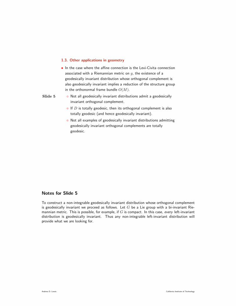
Slide 5
1.3. Other applications in geometry
• In the case where the affine connection is the Levi-Civita connection
associated with a Riemannian metric on g, the existence of a
geodesically invariant distribution whose orthogonal complement is
also geodesically invariant implies a reduction of the structure group
in the orthonormal frame bundle O(M).
◦ Not all geodesically invariant distributions admit a geodesically
invariant orthogonal complement.
◦ If D is totally geodesic, then its orthogonal complement is also
totally geodesic (and hence geodesically invariant).
◦ Not all examples of geodesically invariant distributions admitting
geodesically invariant orthogonal complements are totally
geodesic.
Notes for Slide 5
To construct a non-integrable geodesically invariant distribution whose orthogonal complementis geodesically invariant we proceed as follows. Let G be a Lie group with a bi-invariant Rie-mannian metric. This is possible, for example, if G is compact. In this case, every left-invariantdistribution is geodesically invariant. Thus any non-integrable left-invariant distribution willprovide what we are looking for.
Andrew D. Lewis California Institute of Technology

Slide 6
• When the affine connection is a left-invariant affine connection on a
Lie group, the symmetric product appears in contexts other than
determining geodesically invariant distributions.
◦ Along any geodesic, one may measure the variation of “nearby”
geodesics with Jacobi fields. A Jacobi field along a geodesic may
be pulled back to the Lie algebra. The equations describing the
evolution of the corresponding Lie algebra element involve the
symmetric product.
Notes for Slide 6
The relationship between the symmetric product and Jacobi fields for left-invariant affine con-nections on Lie groups is not well understood. It is merely a computational artifact at themoment.
Andrew D. Lewis California Institute of Technology

Slide 7
2. Geodesic invariance in control of mechanical
systems
2.1. Simple mechanical control systems
• The data for a simple mechanical control system is:
1. A Riemannian metric g on an n-dimensional configuration
manifold Q (describes the kinetic energy).
2. A function V on Q (describes potential energy). Today V = 0.
3. m one-forms F 1, . . . , Fm on Q (describe the input forces). We
shall use Ya = (F a)♯.
Notes for Slide 7
The one-forms F 1, . . . , Fm are the primitive objects which describe the forces. That is to say,the objects in physics which one typically calls forces are naturally one-forms. Nevertheless, it isthe vector fields we actually use in computations.
Andrew D. Lewis California Institute of Technology
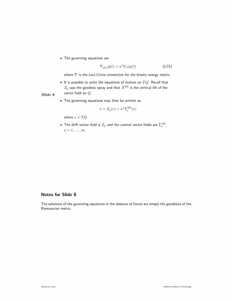
Slide 8
• The governing equations are
∇q(t)q(t) = uaYa(q(t)) (LCS)
where ∇ is the Levi-Civita connection for the kinetic energy metric.
• It is possible to write the equations of motion on TQ. Recall that
Zg was the geodesic spray and that X lift is the vertical lift of the
vector field on Q.
• The governing equations may then be written as
v = Zg(v) + uaY lifta (v)
where v ∈ TQ.
• The drift vector field is Zg and the control vector fields are Y lifta ,
a = 1, . . . ,m.
Notes for Slide 8
The solutions of the governing equations in the absence of forces are simply the geodesics of theRiemannian metric.
Andrew D. Lewis California Institute of Technology
Slide 9
2.2. Configuration controllability of (LCS)
• Let q0 ∈ Q, T > 0, and let U be a neighbourhood of q0. Define
RUQ(q0, T ) = {q′ ∈ Q | there exists a solution
(q, u) of (LCS) which is at q0 at rest
at t = 0 and at q′ (not necessarily at rest)
at t = T and q(t) ∈ U}
and RUQ(q0,≤ T ) =
⋃
0≤t≤T RUQ(q0, t).
• We say that (LCS) is locally configuration accessible at q if
RUQ(q,≤ T ) contains an open subset of Q for each U and each T
sufficiently small.
Notes for Slide 9
Observe that we always start at rest. For the systems we are considering, this is equivalent tostarting at an equilibrium point. It is worth emphasising that we do not restrict ourselves byasking that the final state have zero velocity.
There is also a notion of controllability in the configuration variables. To save confusion, wedo not mention these things here. However, we do have results for configuration controllability.We refer the reader to [Lewis 1995] for the details.
Observe that our controllability definitions are the natural modifications of the usual con-trollability definitions from nonlinear control theory. The modification is that we are no longerlooking at the states of the system but rather just the configurations. This is a physically naturalthing to do, and, as we shall see, also roots out the pertinent mathematical structure of thesystem.
Andrew D. Lewis California Institute of Technology
Slide 10
2.3. A simple example
• Consider the “robotic leg” below
• Q = S1 × S
1 × R+ and
g = Jdθ ⊗ dθ +mr2dψ ⊗ dψ +mdr ⊗ dr
where m is the mass of the ball and J is the moment of inertia of
the body.
• For this example ask the following question:
Starting at a given configuration at rest, which configurations
are accessible by applying suitable combinations of the force
and torque?
Notes for Slide 10
This example, though simple, captures a few important issues involved in our controllabilitydefinitions and computations.
1. If we think of this as a control system on TQ, then this control system is not controllable.The reason for this is that the system, even with inputs, preserves angular momentumand so the solutions must evolve on surfaces of constant angular momentum. In spite ofthis, the system is locally configuration accessible. So in this example our controllabilitydefinitions capture something that the usual definitions fail to capture.
2. This system is more than locally configuration accessible. It is actually controllable. Thatis to say, we can steer the system from one configuration to another. We will not discussthis here, but we refer the reader to [Lewis 1995] for a discussion of related issues.
Andrew D. Lewis California Institute of Technology

Slide 11
2.4. Decompositions for simple mechanical control systems
• Denote Y = {Y1, . . . , Ym}.
• Denote by Cver the smallest geodesically invariant distribution
containing Y.
• Denote by Chor the smallest totally geodesic distribution containing
Y.
2 Theorem: Let q ∈ Q.
(i) The set of velocities accessible from q is an open subset of the
vertical lift of Cver.
(ii) RUQ(q,≤ T ) is an open subset of the integral manifold through q
of Chor.
• The symmetric product is important in proving this result.
Notes for Slide 11
Note that (LCS) is locally configuration accessible at q if rank((Chor)q) = dim(Q).Theorem 2 captures explicitly how the geometry of simple mechanical control systems appears
in the controllability of these systems. It is interesting to see how the notion of geodesic invarianceappears in the result. We mention, without going into details, that the symmetric product wasthe crucial ingredient in arriving at this theorem.
Andrew D. Lewis California Institute of Technology

Slide 12
• Recall that the orthogonal complement of a totally geodesic
distribution is totally geodesic.
• Denote by F the foliation associated with Chor and by F⊥ the
foliation associated with C⊥hor
.
• This defines (at least locally) the following decompositions.
Q
||②②②②②②②②
!!❈❈
❈❈❈❈
❈❈
Q/F⊥ Q/F
• The system on Q/F⊥ is locally configuration accessible.
• The dynamics on Q/F represent “configuration uncontrollable”
dynamics.
• Almost all of the above carries through for general affine
connections, not just Levi-Civita connections. Who cares??
Notes for Slide 12
By “configuration uncontrollable” we mean that, starting at zero velocity, we cannot throughany application of inputs, affect these variables.
Andrew D. Lewis California Institute of Technology

Slide 13
3. Geodesic invariance in constrained mechanics
• Linear constraints in mechanics typically model “rolling without
slipping” (e.g., wheels). The constraint is a distribution D on Q.
• For example, consider the rolling penny:
At each configuration q = (x, y, θ, ψ), Dq describes the directions
the system may move without violating the constraint.
Notes for Slide 13
One may consider more general types of constraints (which are nonlinear in velocity). We arenot sure how or if our methods may be applied to those problems.
Andrew D. Lewis California Institute of Technology

Slide 14
• D⊥ is the orthogonal complement of D and P : TQ→ TQ is the
projection onto D and P ′ : TQ→ TQ is the projection onto D⊥.
• For the Lagrangians we are considering (L = KE), the constrained
equations of motion are (using the Lagrange-d’Alembert principle)
∇q(t)q(t) = λ(t)
P ′(q(t)) = 0
where λ is a section of D⊥ (the constraint force).
Notes for Slide 14
What we present here is a generalisation of work of Bloch and Crouch [1995].Everything we say in this section may be generalised appropriately for arbitrary affine con-
nections.The Lagrange-d’Alembert principle is the appropriate variational principle for mechanical
systems with constraints. There is actually some debate over this, and we refer the readerto [Lewis and Murray 1995] for a discussion of these issues.
In the classical development of the equations of motion for constrained systems, λ is aLagrange multiplier.
Andrew D. Lewis California Institute of Technology

Slide 15
• By covariantly differentiating the constraints we may solve for the
constraint force to arrive at the equivalent equations
∇q(t)q(t) + (∇q(t)P′)(q(t)) = 0
=⇒ ∇′q(t)q(t) = 0
where ∇′ is a new affine connection defined by
∇′XY = ∇XY + (∇XP
′)(Y ).
• This connection has the property that ∇′XY is a section of D for
every vector field X and every section Y of D. In particular,
◦ D is geodesically invariant with respect to ∇′, and
◦ the affine connection ∇′ restricts to a vector bundle connection
in D.
Notes for Slide 15
The object ∇′ is an affine connection since (X,Y ) 7→ (∇XP′)(Y ) defines a (1, 2) tensor field.
It is interesting to see that we have defined ∇′ so that D is geodesically invariant. In thiscase, it is also true that the affine connection reduces to a connection in D. This is not true,however, for arbitrary geodesically invariant distributions, even in the Levi-Civita case.
Speaking of Levi-Civita connections, it is interesting to ask when the connection ∇′ is aLevi-Civita connection. The answer is best obtained by looking at the holonomy groups of ∇′.This will be future work.
Andrew D. Lewis California Institute of Technology

Slide 16
• Since our control theoretic setup for unconstrained systems extends
to general affine connections, we may directly apply those methods
to problems with constraints.
• The control problem is
∇′q(t)q(t) = uaP (Ya(t)) (CLCS)
• We have the following result:
3 Theorem: Let q ∈ Q. The set of configurations of (CLCS)
accessible from q with zero initial velocity is an open subset of the
leaf through q of the smallest totally geodesic (w.r.t. ∇′!)
distribution containing the inputs.
Notes for Slide 16
The fact that one only has to consider the projection of the inputs to D make sense since thepart of the force in D⊥ will be absorbed by the Lagrange multiplier.
Andrew D. Lewis California Institute of Technology

Slide 17
• We may perform a sanity check of our constructions and results.
◦ If D is integrable then
(X,Y ) 7→ −(∇XP′)(Y )
is the second fundamental form for the integral manifolds. In this
case ∇′ reduces to the induced Levi-Civita connection on the
leaves.
◦ If D is totally geodesic then ∇XP′ = 0 for every vector field X .
In this case ∇′ = ∇.
Notes for Slide 17
Recall that the second fundamental form is derived when one decomposes the original affineconnection into its tangential and normal pieces. It is easy to show that (∇XP
′)(Y ) is orthogonalto D when X and Y are in D and so it easily follows that it must be (up to sign) the secondfundamental form. Also recall that the second fundamental form vanishes when the submanifoldin question is totally geodesic as, in this case, the geodesics of the induced affine connectionagree with those of the full system.
Andrew D. Lewis California Institute of Technology

Slide 18
◦ Since
1. we can only reach configurations contained in leaves of the
smallest totally geodesic distribution containing the inputs,
and
2. the inputs are contained in D,
the set of reachable configurations is contained in the leaves of
the involutive closure of D. That is, we cannot reach more
configurations that the constraints will allow.
Notes for Slide 18
These sanity checks give us no surprising results, but at least indicates that our constructioneasily recovers the obvious results.
Andrew D. Lewis California Institute of Technology

Slide 19
4. Wrap up
• We have explored the relationship of the symmetric product with
the concept of geodesic invariance for affine connections.
• These ideas have applications in geometry, mechanics (with
constraints), and control theory for mechanical systems.
Andrew D. Lewis California Institute of Technology
Slide 20
• Future work includes:
◦ On the geometry side we would like to fully understand how the
presence of geodesically invariant distributions affects the
structure of the affine connection (especially its holonomy
groups).
◦ On the control theory side, we would like to see if an
understanding of the symmetric product can be useful in
designing controllers for mechanical systems.
◦ For systems with constraints, we would like to understand the
relationship of ∇′ with other recent work on constrained systems.
Notes for Slide 20
We have briefly stated a few preliminary results about how one may reduce the structure groupof O(M) in the presence of a distribution which is geodesically invariant and whose orthogonalcomplement is geodesically invariant. However, a more general understanding might be valuable.
In nonlinear control theory, understanding the Lie bracket has enabled certain researchers toimplement control laws for certain classes of control systems, especially nonholonomic systems.It would be interesting to see if a similar benefit may be gained by better understanding thesymmetric product.
Recent work for constrained systems includes that of Bloch, Krishnaprasad, Marsden, andMurray [1996]. Understanding their momentum equation in terms of our connection ∇′ may beinteresting.
Andrew D. Lewis California Institute of Technology
References
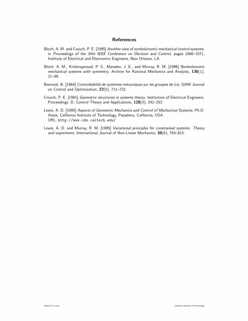
Bloch, A. M. and Crouch, P. E. [1995] Another view of nonholonomic mechanical control systems,in Proceedings of the 34th IEEE Conference on Decision and Control, pages 1066–1071,Institute of Electrical and Electronics Engineers, New Orleans, LA.
Bloch, A. M., Krishnaprasad, P. S., Marsden, J. E., and Murray, R. M. [1996] Nonholonomic
mechanical systems with symmetry, Archive for Rational Mechanics and Analysis, 136(1),21–99.
Bonnard, B. [1984] Controllabilite de systemes mecaniques sur les groupes de Lie, SIAM Journalon Control and Optimization, 22(5), 711–722.
Crouch, P. E. [1981] Geometric structures in systems theory, Institution of Electrical Engineers.Proceedings. D. Control Theory and Applications, 128(5), 242–252.
Lewis, A. D. [1995] Aspects of Geometric Mechanics and Control of Mechanical Systems, Ph.D.thesis, California Institute of Technology, Pasadena, California, USA.URL: http://www.cds.caltech.edu/
Lewis, A. D. and Murray, R. M. [1995] Variational principles for constrained systems: Theory
and experiment, International Journal of Non-Linear Mechanics, 30(6), 793–815.
Andrew D. Lewis California Institute of Technology
![NOTES ON SCALE-INVARIANCE AND BASE-INVARIANCE FOR … · arXiv:1307.3620v1 [math.PR] 13 Jul 2013 NOTES ON SCALE-INVARIANCE AND BASE-INVARIANCE FOR BENFORD’S LAW MICHAŁ RYSZARD](https://static.fdocuments.net/doc/165x107/5aee16367f8b9a45569086fd/notes-on-scale-invariance-and-base-invariance-for-13073620v1-mathpr-13-jul.jpg)