THE STRUCTURE OF APPLIED GENERALEQUILIBRIUM MODELS

Victor GinsburghandMichie! Keyzer

The MIT PressCambridge, MassachusettsLondon, England

Introduction

This book describes the structure of general equilibrium models. It is writtenfor the researcher who intends to construct or study applied generalequilibrium (AGE) models and has a special interest in their theoreticalbackground. Both general equilibrium theory and AGE modeling continueto be active fields of research, but the styles of presentation differ greatly.Whereas the applied model builder often finds the style of theoretical papersinaccessible, the theoretician can hardly recognize the concepts he is used toin the list of equations of applied models. The main purpose of the book isto present the theoretical models in a unified way and to indicate how themain concepts can find their way into applications.

To make the models more accessible and their structure more transpar-ent, we unify the presentation in four ways. First, we use standardized,though possibly not the weakest, assumptions on basic model componentslike utility functions and production sets (chapters 1 and 2), and we onlydeviate from the standard when the topic requires it. Second, in chapter 3we define five basic formats to represent and to analyze the same model. Forevery specific model to be discussed in chapters 4 to 12, we apply the formatthat proves most convenient. Third, beside fixed point theorems (appendixA.4), we almost exclusively use theorems from the theory of convexprogramming as mathematical background (appendixes A.1 to A.3). Finally,every model in chapters 4 to 12 analyzes a topic within a common basicscheme, as follows:

1. The chapter starts introducing the topic (e.g., taxes or finite horizondynamics) and then proceeds with the discussion of the issues related to thetopic itself as well as its incorporation in a general equilibrium model. Thismay require nonstandard assumptions (e.g., relaxing convexity).

2. Existence proofs are given, using the most convenient format defined inchapter 3. The proofs are not meant as a theoretical contribution andmainly serve to highlight the roles of the various assumptions and toindicate how the fixed point mapping can be set up for computing a solutionvia fixed point algorithms. Issues in computation are briefly dealt with inappendixes A.7 to A.9.

3. Various properties of the equilibrium solution of the model are analyzed,with a focus on efficiency. We derive conditions under which the inefficien-cies due to specific imperfections (taxes, price rigidities, external effects) canbe reduced through Pareto-improving reforms. However, these reforms onlyrepresent an idealized situation, since they require losers to be compensatedand all imperfections to be reduced simultaneously.

4. Policy reforms can rarely eliminate or even reduce all imperfections atthe same time. Therefore their consequences cannot be predicted fromtheory alone, and numerical simulation is called for. This requires construct-

IntroductionXIV

ing applied models that can be used to run alternative scenarios. Everychapter ends with a section that describes how applied models that incor-porate ,the theoretical concepts can be built and briefly surveys existingapplications.

The following limitations should be mentioned:

1. For clarity of exposition, the topics will often be treated in isolation. Forexample, we limit the presentation of finite and infinite horizon dynamics tothe case of the cl~sed economy. Occasionally some issues need to be treatedtogether (e.g., taxes, tariffs, and foreign trade in chapter 5).

2. In chapter 2 we compare several analytical forms (CES, translog, etc.) forthe functions that should be estimated econometrically, but in the sectionson applications, we do not enter into the details of these specifications.

3. We sketch the framework for national and social accounting that isneeded as a database (the social accounting matrix, SAM) to calibrate amodel, but we hardly discuss the elaborate process that leads from statisticalpublications to such a database.

4. Computation of equilibria has received much attention in the early yearsof AGE modeling. Advances in computing capacity and speed as well as theavailability of user friendly packages, such as GAMS, have almost elimin-ated computational concerns for most applications. Therefore computa-tional issues are only treated briefly in appendixes.

5. The numerical solutions of AGE models should be made easily interpre-table for the policy analyst who will be reluctant to decipher the standardprintings from software packages. The presentation should thus be cus-tomized, and the results should be cast in the form of tables the analyst isfamiliar with. Deriving such tables for every model is hardly meaningfulwithout a numerical illustration, and giving this in every chapter wouldcause excessive duplication.

We overcome some of these limitations and avoid repetition by descri-bing, in appendix B, a complete numerical application in GAMS language,incorporating taxes, trade, price rigidities, buffer stocks, transportationcosts, and simple dynamics. The application uses simple functional formsand yields social and national accounts in report quality form.!

To summarize, chapters 1 to 3 and appendix A set the framework for thetopics covered in chapters 4 to 12. Chapter 1 provides an elementary butalmost comprehensive treatment of the competitive model. It ends, insection 1.5, with an overview of the properties that could be relaxed so asto make the model more useful for policy analysis and introduces thesubjects covered in chapters 4 to 12. Chapter 2 deals with relatively standardelements of the theory of producer and consumer behavior, most of which

Introduction

can be found in textbooks such as Varian's Microeconomic Analysis. Thereader who is familiar with this material can proceed to section 2.3, whichsummarizes the microeconomic assumptions that are used in later chapters.Section 2.4 presents results on welfare analysis that are needed in proofs.Chapter 3 describes the basic formats and introduces the methods of proofused in the book. .Its last section discusses the main steps in constructing anumerical application and gives a full GAMS application for the simplestpossible model. The reader may choose freely the order in which he wantsto study the topics covered in chapters 4 to 12. Occasionally he may haveto consult material from earlier chapters and from appendix A, and this willbe pointed out explicitly when needed.

A user's guide and library of GAMS-models (Keyzer 1997) accompanythis volume. Both are freely accessible at the MIT Press Internet site(http://www.mitpress.mit.edu). The guide extends the material covered inappendix B. The library contains a set of computer programs with illus-trative applications for most of the models covered in chapters 3 to 12 ofthis book, except for the infinite horizon m,odels of chapter 8.

Notation

;i

We denote the n-dimensional real space by Rft, the nonnegative orthant byR~, and the positive orthant by R~ +. Let x and y be two vectors in Rft. Thefollowing notations are equivalent:

Enumeration all h ~ h = 1,..., n

n

Summation ~hXh == L xhh=l

If and only if iff or ~

Complementary slackness (x ~ 0 .L Y ~ 0) ~ (x ~ 0, xy = 0, y ~ 0)

Inner productl xy == X' Y == ~hXhYh

Inequality x ~ y~xh ~ Yh for all h, and similarly for ~;x > Y ~ Xh > Yh for all h, and similarly for <.

Partial derivative (Jacobian) F'(x) == of(x)jox

Fixed point or equilibrium superscript *

Optimal value of a variable2 superscript 0

Vector norm3 Ilxllp == (~~= llxhIP)l/p for given 1 ~ p < 00;Ilxlloo == maxl~h~nlxhl, for the limiting case;Ilxll == Ilxllp for some p to be specified.

Matrix norm IIAII == suPllxll=lllAxll

Notation in the Mathematical Program

The notation will be introduced by means of an example. Define thefunction u: X c Rn -+ R and the sets Yj c Rn, j = 1,. .., J, and consider themathematical program:

max u(x),

x;:?:O,Yj,allj,

subject to

x ~ ~jYjYjE}j.(P),

For simplicity we write "max" instead of "sup" because we only considerprograms for which the maximum will be attained. The choice variables xand Y j are placed under the maximand. Here x is constrained to be

1. When no confusion is possible, we avoid using the transposition sign for inner productsand for premultiplication of a matrix by a vector.2. When no distinction with equilibrium values is needed, the superscript * is also used.

3. More general definitions can be used. Here we restrict ourselves to {p-norms.

Notationxx

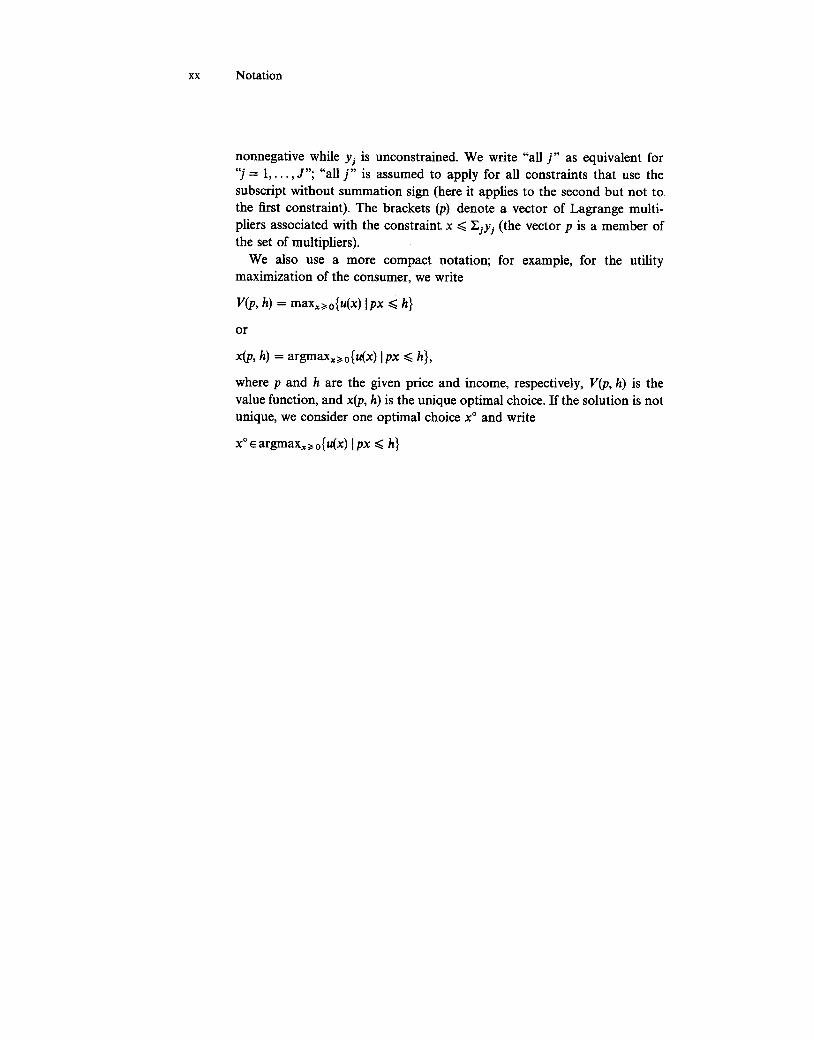
nonnegative while Yj is unconstrained. We write "all j" as equivalent for')" = 1,..., J"; "all j" is assumed to apply for all constraints that use the

subscript without summation sign (here it applies to the second but not tothe first constraint). The brackets (P) denote a vector of Lagrange multi-pliers associated with the constraint x ~ ~jYj (the vector p is a member ofthe set of multipliers).

We also use a more compact notation; for example, for the utilitymaximization of the consumer, we write

V(p, h) = maxx~o{u(x) Ipx ~ h}

or

x(p, h) = argmaxx~o{u(x) Ipx ~ h},

where p and h are the given price and income, respectively, V(p, h) is thevalue function, and x(p, h) is the unique optimal choice. If the solution is notunique, we consider one optimal choice XC and write

xOEargmaxx~o{u(x) Ipx ~ h}

Competitive Equilibrium

In this chapter we describe an economy, say, of a village, a town, or acountry, that does not entertain trading relations with an outside world. Wecall this a closed economy.

After introducing basic concepts in section 1.1, we prove existence ofequilibrium in the simplest possible aggregate framework, without referenceto individuals' behavior, and we discuss computation of equilibrium andproperties like multiplicity and stability in section 1.2. In section 1.3 weimpose a first set of assumptions on the behavior of producers andconsumers and show that under these assumptions, a competitive equilib-rium exists. Section 1.4 is devoted to the welfare properties of equilibriumallocations. Finally, section 1.5 points to the need for extensions that willyield an applied general equilibrium model with a more realistic structure.

1.1 Basic Concepts

1.1.1 Commodities and Agents; Demands and Supplies

utus consider an economy with r commodities indexed by k = 1,2,...,r.The commodity space is thus an r-dimensional space, denoted by Rr, and allvectors belong to that space.

An orange available today in New York is more or less the same as anorange in Marseilles tomorrow, but each will be defined as a differentcommodity in a general equilibrium model, which distinguishes commodi-ties by location and date of delivery. By definition, each commodity k willbe traded at a single price Pk. Agents are characterized by preferences overcommodities and by capabilities to satisfy these preferences through actionslike production, purchases, sales, storage, and consumption, now or in thefuture. This situation may be formalized by representing each agent asmaximizing his utility subject to technological and trading constraints. Inthe simplest case the budget constraint, which requires expenditure not toexceed revenue, is the only restriction on exchanges. Under these conditionsand some specific assumptions to be discussed later on, we can decomposethe decisions made by each agent into two subproblems:! profit maximiza-tion subject to technological constraints, and utility maximization subject toa budget constraint.

These subproblems enable us to consider two types of agents who makedecisions: producers (or firms) and consumers. There will be n producers,indexed by j = 1, 2,..., n who will produce (and sell) commodities using(and buying) some other commodities, like labor, steel, and machines. LetY j(P) be the production plan of producer j, where P denotes the price vector;outputs will carry a positive sign and inputs a negative sign. There will be

1. See Koopmans (1957).

2 Chapter 1

m consumers, indexed by i = 1,2,..., m. Every consumer offers for sale hiscommodity endowment Wi and expresses the wish to buy a commoditybundle Xi(P) at given prices p.

We define the excess demand vector z(P) as

z(P) = kiXi(P) -kjYj(P) -kiWi.

The typical component Zk(P) of this vector will represent the excess ofdemand over supply (which includes the initial endowment) of commodity k.

A natural solution concept is to require that no commodity be in excessdemand; otherwise, some agents would not be able to carry out theirdemands. We accept, however, that there can be excess supply for somecommodities, which can be disposed of freely (the free disposal assumption).An excess demand equilibrium is then defined as follows:

DEFINmON 1.1 (Excess demand equilibrium) The price p* ~ 0, p* # 0,and the excess demand z(p*) define an excess demand equilibrium ifz(p*) ~ O.1.1.2

The Behavior of Producers and Consumers

Our description of the agents' behavior starts with the assumption thatprices exist for all commodities and that all agents take these prices as given,none of them being sufficiently "large" or "important" to think that he caninfluence a price, even less set a price. Prices are thus considered as signalson the basis of which agents compute their plans. Such an institutionalsetting is commonly referred to as perfect competition.

Production Plans

Each producer j is endowed with a technology, represented by a set 1),which belongs to Rr and is the set of feasible production plans. A producerformulates a production plan Y j that must be feasible: This is expressed asY j E 1). Obviously further assumptions that characterizeihe mathematicalproperties of the set 1) are needed. The competitive model assumes that fromthe set of feasible plans Y j' the producer chooses those that maximize hisprofit, defined as LkPkYjk or PYj.

The problem of producer j can thus be stated as follows: Given the pricevector P, and the technological set 1), producer j chooses Y j so as to max-imize profits PY j subject to a feasibility constraint Y j E 1), or

llj(P) = maxYJ{PYj I YjE 1)}, (1.1)

where llj(P) is the resulting maximal profit.

Competitive Equilibrium

Consumption Plans

The choice made by consumer i is restricted in two ways. First, hisconsumption plans need to be feasible: He cannot consume negativequantities of any commodity: XiER'+. Second, he is faced with a budgetconstraint: He cannot spend more than his income hi. Since at given pricesp, a consumption plan Xi costs PXi, his budget constraint can be written as

PXi ~hi.

The income hi of the consumer consists of two parts: The proceeds proi ofselling the endowment roi and distributed profits. The latter are defined asfollows: It is assumed that consumer i owns a nonnegative share (}ij in firmj and that he receives dividends (}ijllj(P) from this firm. All profits aredistributed so that Li(}ij = 1 for every j. Consumer i's income is now

h. = Pro. + L.(}..ll. (P)., , J 'J J

Consumer i is also characterized by a utility function Ui(XJ, which associatesto every consumption plan Xi a utility level Ui(XJ; under further assumptionson Ui(XJ, this makes it possible to consistently rank alternative consumptionbundles.

The problem of consumer i can now be stated as follows: Given the pricevector P and the revenue hi, consumer i chooses Xi so as to maximize hisutility Ui(XJ subject to a feasibility constraint Xi ;;:!: 0 and to his budgetconstraint PXi ~ hi, or

maxx/~O{Ui(XJ IpXi ~ hJ.

1.1.3 General Competitive Equilibrium

(1.2)

The excess demand equilibrium of definition 1.1 is a general equilibriumbecause it covers all agents and all commodities of the economy. We cannow define a general competitive equilibrium as an excess demand equilib-rium, in which producers and consumers behave according to (1.1) and (1.2),

respectively.

DEFINITION 1.2 (General competitive equilibrium) The allocation yj, all j,xf, all i, supported by the price vector p* ~ 0, p* :;.!: 0 is a general competi-tive equilibrium if the following conditions are satisfied:

1. For every producer j, yj solves maXyj{p*YjIYjE }j}.

2. For every consumer i,xt solves maXXi~O{Uj(xJ Ip*Xj ~ ht}, where ht =P*Wj + I:jlJjjp*yj.

3. All markets are in equilibrium, I:jxt -I:jyj -Ejwj ~ O.

4 Chapter

In definition 1.2 there are four components. First, agents have behavioralrules that they follow to compute their optimal decisions. Second, in doingso, they take into account signals, without trying to affect these: Producersreact on prices only, consumers take into account prices and their income.Third, there is a price for every commodity, so a competitive market existsfor every commodity. Fourth, there are conditions on excess demands,which agents do not take into account when making their decisions andwhich are satisfied in equilibrium.

Characteristics of a General Competitive Equilibrium

So far, endowments Wi and shares in profits f)ij are the only explicitparameters. In applied models other parameters like tax rates or institu-tional rigidities will appear, and the model. will be used to compute solutionswhen variations are imposed on some of these parameters. When analyzingthe response of the model to such changes, several issues have to beaddressed. To introduce these, we consider the response of the systemz(p, w) ~ 0 to variations in W only, where W = (WI' W2,..., rom) is the vectorof endowments of all consumers.

Various questions now come up: (1) What are natural properties forz(p, w) (assumptions)? (2) Does the system z(p, W) = 0 have a solution withnonnegative prices (existence)? (3) How many such solutions are there(multiplicity)? (4) Do we know anything on the direction of change of pricesand allocations when W changes (general properties of z(p, w»? (5) How tocompute solutions given a numerical specification of z(p, w)? (6) Are somepolicy changes "better" than others (welfare analysis)? Finally, when build-ing an applied general equilibrium model, the main issue is (7) how tospecify numerically the model (empirical implementation). We will discussthese questions by turns.

1.2 Excess Demand Equilibrium

1.2.1 Assumptions on the Excess Demands

We now formulate assumptions on the excess demand function z(P), alongthe lines of Arrow and Hahn (1971, ch. 2). In section 1.3 we will specifyassumptions on individual agents and the properties of the excess demandfunction will follow from there:

ASSUMPTION Zl (Sipgle-valuedness and continuity) z(P) is a single-valuedand continuous function, which is defined for p ~o, p # 0.2

2. We use the following notation: p ;1; 0 means that Pk ;1; 0 for all kE~~~~ mean thatPk > 0 for some k, P > 0 means that Pk > 0 for all k.

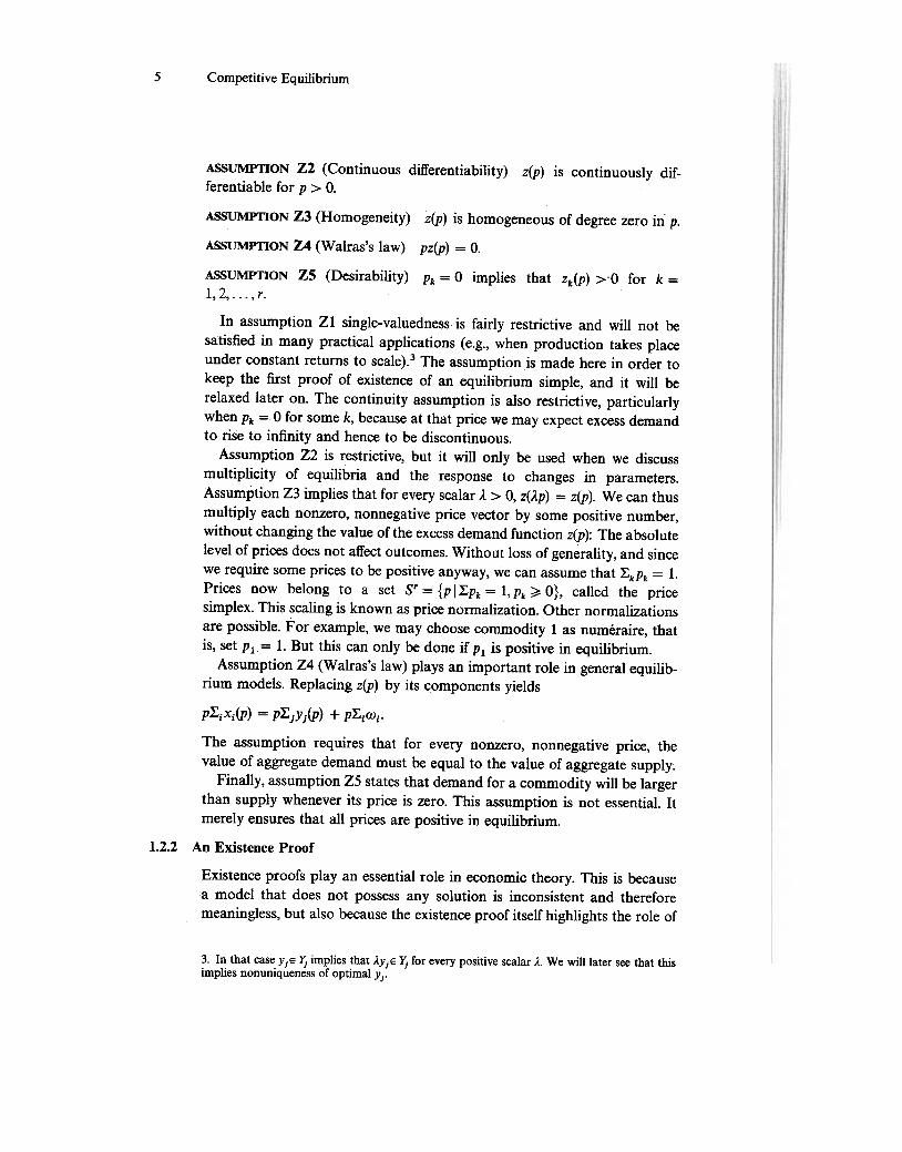
5 Competitive Equilibrium

ASSUMPTION Z2 (Continuous differentiability) z(P) is continuously dif-ferentiable for p > O.

ASSUMPTION Z3 (Homogeneity) z(P) is homogeneous of degree zero in p.

ASSUMPTION Z4 (Walras's law) pz(P) = O.

ASSUMPTION Z5 (Desirability) Pk = 0 implies that Zk(P) >"0 for k =1,2, ..., r.

In assumption Zl single-valuedness is fairly restrictive and will not besatisfied in many practical applications (e.g., when production takes placeunder constant returns to scale).3 The assumption is made here in order tokeep the first proof of existence of an equilibrium simple, and it will berelaxed later on. The continuity assumption is also restrictive, particularlywhen Pk = 0 for some k, because at that price we may expect excess demandto rise to infinity and hence to be discontinuous.

Assumption Z2 is restrictive, but it will only be used when we discussmultiplicity of equilibria and the response to changes in parameters.Assumption Z3 implies that for every scalar J. > 0, z(J.p) = z(P). We can thusmultiply each nonzero, nonnegative price vector by some positive number,without changing the value of the excess demand function z(P): The absolutelevel of prices does not affect outcomes. Without loss of generality, and sincewe require some prices to be positive anyway, we can assume that ~kPk = 1.Prices now belong to a set sr = {p I ~Pk = 1, Pk ~ O}, called the pricesimplex. This scaling is known as price normalization. Other normalizationsare possible. For example, we may choose commodity 1 as numeraire, thatis, set PI = 1. But this can only be done if PI is positive in equilibrium.

Assumption Z4 (Walras's law) plays an important role in general equilib-rium models. Replacing z(P) by its components yields

P}:;iXi(P) = P}:;jYj(P) + P}:;i(()i.

The assumption requires that for every nonzero, nonnegative price, thevalue of aggregate demand must be equal to the value of aggregate supply.

Finally, assumption Z5 states that demand for a commodity will be largerthan supply whenever its price is zero. This assumption is not essential. Itmerely ensures that all prices are positive in equilibrium.

1.2.2 An Existence Proof

Existence proofs play an essential role in economic theory. This is becausea model that does not possess any solution is inconsistent and thereforemeaningless, but also because the existence proof itself highlights the role of

3. In that case YjE:!J implies that AYjE:!J for every positive scalar A. We will later see that thisimplies nonuniqueness of optimal Yj.

6 Chapter 1

the assumptions made and, by that, facilitates the search for weakerassumptions. In doing so, it enlarges the field to which the theory applies.

The applied modeler may think that he can dispense of existence proofsbecause a reasonable model can always be calibrated so as to possess asolution. However, such a calibration will not help when the modeler seeksto compute a new solution after having changed the value of someparameter. Then he needs to know the range of parametric variations forwhich a solution will exist at all. The theoretical assumptions limit the rangeof variations of these parameters, and the existence proof makes clear whythese restrictions are needed. Finally, the existence proof is useful because itwill in general construct a fixed point mapping that can serve as the basisof the fixed point algorithms that solve the model numerically.

We will now prove that an equilibrium exists in this economy, using theassumptions made in section 1.2.1. The proof of this basic result rests on afixed point theorem, due to Brouwer, that states that a continuous functionG that maps a compact convex set A into itself (G: A -+ A) has a fixed pointx*, that is, a point such that x* = G(X*}.4

Hence Brouwer's theorem imposes three requirements: (1) the functionG(x} should be continuous, (2) it should map from a compact, convexdomain A, (3) the mapping should be "into itself': The range A should bethe same as the domain. We illustrate the role of each of these requirements.In figure 1.la we draw a function that meets all the requirements with theunit interval as the set A. There are three fixed points (intersections with the450 line). Note first that unless the function is tangent to the 450 line, thenumber of fixed points will always be finite, and there will be at least oneintersection. Then, unless the function starts at (0,0) and ends at (1, 1), thenumber of fixed points must be odd. In figure 1.lb the mapping is not singlevalued (it is not a function but a correspondence); nevertheless, it maps fromA into A and is convex valued (it is obviously so when single valued, but italso is at XO where it is set valued, since the interval BB' is a convex set). Inthis case a fixed point will exist, but now by virtue of the Kakutani theoremsinstead of the Brouwer theorem. In figure 1.lc the correspondence iscompact and maps into A, but it is not convex valued (and not continuous)at XO and there is no fixed point. Figure 1.ld shows that the threerequirements are sufficient but not necessary: A fixed point exists, thoughthe function is not continuous, not defined everywhere, not compact valued(it goes to infinity), and does not map into itself (C does not lie in A). Infigure 1.le the domain of the function is compact, and the function iscontinuous, so its range is compact. But the range is not contained in the

4. See theoremA.4.! in the mathematical appendix A.

5. See theorem A.4.2.

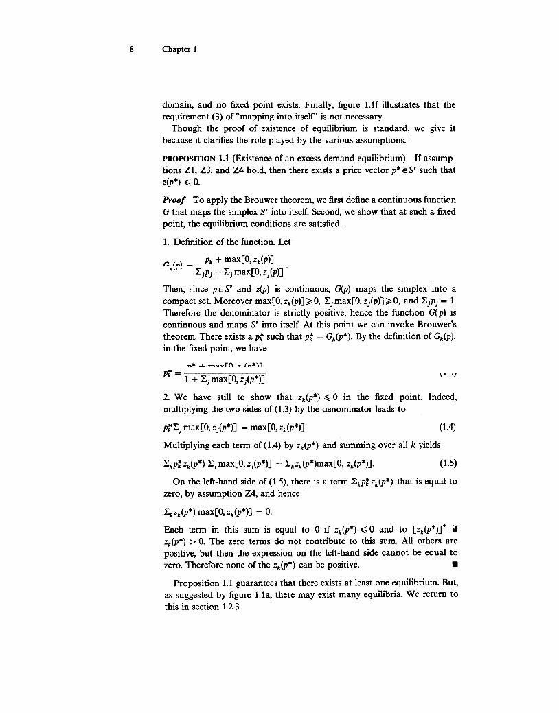
8 Chapter 1

domain, and no fixed point exists. Finally, figure 1.1f illustrates that therequirement (3) of "mapping into itself' is not necessary.

Though the proof of existence of equilibrium is standard, we give itbecause it clarifies the role played by the various assumptions.

PROPosmON 1.1 (Existence of an excess demand equilibrium) If assump-tions Zl, Z3, and Z4 hold, then there exists a price vector p* E S' such thatz(p*) ~ o.

Proof To apply the Brouwer theorem, we first define a continuous functionG that maps the simplex S' into itself. Second, we show that at such a fixedpoint, the equilibrium conditions are satisfied.

1. Definition of the function. Let

GL(lJ) = Pk + max[O, Zk(P)]-A~' ~jPj + ~jmax[O'Zj(P)] .

Then, since P E sr and z(P) is continuous, G(p) maps the simplex into acompact set. Moreover max[O'Zk(P)]~O, ~jmax[O,zj(P)]~O, and ~jPj = 1.Therefore the denominator is strictly positive; hence the function G(p) iscontinuous and maps sr into itself. At this point we can invoke Brouwer'stheorem. There exists ap: such that pt = Gk(P*). By the definition of Gk(P),in the fixed point, we have

p: + max[O, Zt(P*)]p* -k -1 + }:;jmax[O,Zj(P*)]. \,".J}

2. We have still to show that Zk(P*) ~ 0 in the fixed point. Indeed,multiplying the two sides of (1.3) by the denominator leads to

pt}:;jmax[O,Zj(P*)] = max[O,zk(P*)]. (1.4)

Multiplying each term of (1.4) by Zk(P*) and summing over all k yields

}:;kPt Zk(P*) }:; j max[O, Z j(P*)] = }:;kZk(P*)max[O, Zk(P*)]. (1.5)

On the left-hand side of (1.5), there is a term }:;kPt Zk(P*) that is equal tozero, by assumption Z4, and hence

}:;kZk(P*) max[O, Zk(P*)] = O.

Each term in this sum is equal to 0 if Zk(P*) ~ 0 and to [Zk(P*)]2 ifZk(P*) > O. The zero terms do not contribute to this sum. All others arepositive, but then the expression on the left-hand side cannot be equal tozero. Therefore none of the Zk(P*) can be positive. .

Propo'sition 1.1 guarantees that there exists at least one equilibrium. But,as suggested by figure 1.1a, there may exist many equilibria. We return tothis in section 1.2.3.

9 Competitive Equilibrium

We note that by the homogeneity assumption Z3 and because wedisregard the case with p = Q, it was possible to normalize prices to thesimplex sr, the compact, convex domain of the mapping. Assumption Z4(Walras's law) was used to prove that the fixed point is an equilibrium.Hence assumptions Zl, Z3, and Z4 are sufficient for existence of anequilibrium. However, models that fail to satisfy some of these may possesssolutions, as was illustrated in figures 1.ld and f.

The intuition behind the artificial function G(p) in the proof is to increasethe price Pk of a commodity that is in excess demand (Zk(P) > 0). However,such a mapping should not be interpreted as a theory of the dynamics ofprice adjustment. Producers and consumers carry out their plans only inequilibrium; the model has no clear "out.of-equilibrium" interpretation; inparticular, no exchange is specified to take place out of equilibrium. Insection 1.2.5 we further discuss the issue when we consider computation of

equilibrium.Since Zk(P*) ~ 0 in equilibrium, we do not exclude strict inequality and

hence allow for excess supply of some commodity. But then, as stated inproposition 1.2, the associated price P: will be zero.

PROPOSmON 1.2 (Free goods) Under assumptions Zl, Z3, and Z4,Zk(P*) < 0 implies that P: = o.

Proof In equilibrium z(p*)~O and p* ~o, so P:Zk(P*)~O for every k. Now,if, for some k, Zk(P*) <0 and P:>O, then P:Zk(P*) <0. However, for Walras'slaw to hold, it must be that P:Zh(P*) > 0 for at least one commodity. Thiscannot happen, since P:Zk(P*) ~ 0 for every k, a contradiction. -

Proposition 1.2 shows that all goods in excess supply have a zero price.Of course in the real world economy, they may have a positive price. Forexample, on the labor market, unemployment may prevail at a positive wagerate. We will return to this in chapter 6.

In the existence proof we do not use assumption Z5. However, whenexcess demand is obtained from aggregation of consumers' and producers'plans, it is difficult to maintain continuity of z(P) if the price of somecommodity is zero. We will make assumptions on consumers' utilityfunctions and endowments that make prices positive in equilibrium. We willbe interested only in goods that carry positive prices and will discard fromour model goods we know to be available freely.

PROPosmON 1.3 (Positive prices) Under assumptions Zl and Z3 to Z5,equilibrium prices p* are positive.

Proof Evidently p: = 0 implies that Zk(P*) > 0 by assumption Z5 and thiscannot be an equilibrium. .

10 Chapter

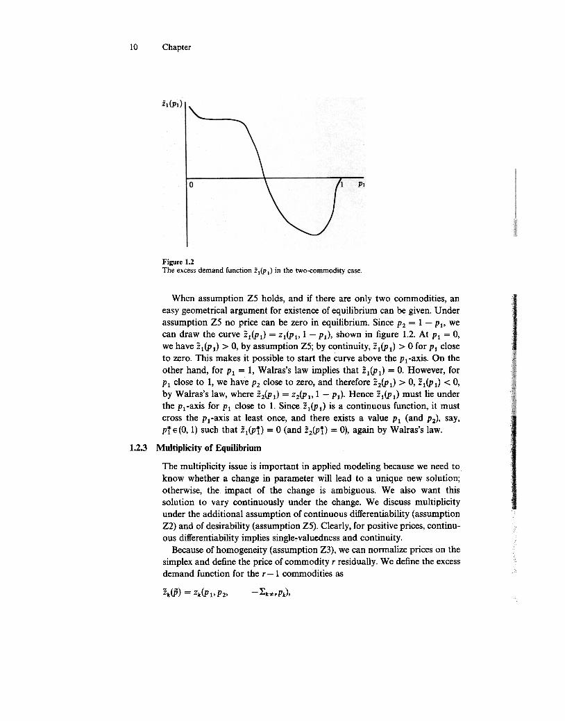
Figure 1.2The excess demand function Zl(Pl) in the two-commodity case.

When assumption Z5 holds, and if there are only two commodities, aneasy geometrical argument for existence of equilibrium can be given. Underassumption Z5 no price can be zero in equilibrium. Since Pz = 1 -PI' wecan draw the curve Zl(Pl) = Zl(Pl' 1 -pJ, shown in figure 1.2. AtPl = 0,we have Zl(PJ > 0, by assumption Z5; by continuity, Zl(PJ > 0 for Pl closeto zero. This makes it possible to start the curve above the Pi-axis. On theother hand, for Pl = 1, Walras's law implies that Zl(Pl) = O. However, forPl close to 1, we have Pz close to zero, and therefore zz(PJ > 0, Zl(PJ < 0,by Walras's law, where zz(PJ = ZZ(Pl' 1 -pJ. Hence Zl(PJ must lie underthe Pi-axis for Pl close to 1. Sincez1(Pl) is a continuous function, it mustcross the Pi-axis at least once, and there exists a value Pl (and pz), say,pTE(O, 1) such that Zl(P!) = 0 (and zz(P!) = 0), again by Walras's law.

1.2.3 Multiplicity of Equilibrium

~

The multiplicity issue is important in applied modeling because we need toknow whether a change in parameter will lead to a unique new solution;otherwise, the impact of the change is ambiguous. We also want thissolution to vary continuously under the change. We discuss multiplicityunder the additional assumption of continuous differentiability (assumptionZ2) and of desirability (assumption Z5). Clearly, for positive prices, continu-ous differentiability implies single-valuedness and continuity.

Because of homogeneity (assumption Z3), we can normalize prices on thesimplex and define the price of commodity r residually. We define the excessdemand function for the r -1 commodities as

-~k*rPJ,Zk(P) = Zk(P l' PZ'

~