The strati ed Cox Procedure - ETH Zurich · The strati ed Cox Procedure Lisa Borsi, Marc Lickes &...
115
The stratified general Cox (SC) model No interaction assumption Comparing: Likelihood, Wald & score test Example Graphical Comparison of the models so far Summary The stratified Cox Procedure Lisa Borsi, Marc Lickes & Lovro Soldo 28. March 2011 Lisa Borsi, Marc Lickes & Lovro Soldo The stratified Cox Procedure
Transcript of The strati ed Cox Procedure - ETH Zurich · The strati ed Cox Procedure Lisa Borsi, Marc Lickes &...

The stratified general Cox (SC) modelNo interaction assumption
Comparing: Likelihood, Wald & score testExample
Graphical Comparison of the models so farSummary
The stratified Cox Procedure
Lisa Borsi, Marc Lickes & Lovro Soldo
28. March 2011
Lisa Borsi, Marc Lickes & Lovro Soldo The stratified Cox Procedure

The stratified general Cox (SC) modelNo interaction assumption
Comparing: Likelihood, Wald & score testExample
Graphical Comparison of the models so farSummary
Recall:
1 Cox PH-Model
- Model from Week 3
h(t,X ) = h0(t)e∑
i βiXi
2 PH-Assumption
- Hazard ration const. over time
HR :=h(t,X ∗)
h(t,X )= const
Explanation of the Formula
Product of two quantities:is called the baseline hazard
Exponential of the sum of and
Baseline hazard is an unspecified functionSemi-parametric modelReason for Cox model being popular
March 11, 2011 16Cox Proportional Hazards Model
th0i iX
X X
p
iii Xthth
10 exp, X
Figure: Definition from Presentation 3
Lisa Borsi, Marc Lickes & Lovro Soldo The stratified Cox Procedure

The stratified general Cox (SC) modelNo interaction assumption
Comparing: Likelihood, Wald & score testExample
Graphical Comparison of the models so farSummary
Recall:
1 Cox PH-Model
- Model from Week 3
h(t,X ) = h0(t)e∑
i βiXi
2 PH-Assumption
- Hazard ration const. over time
HR :=h(t,X ∗)
h(t,X )= const
p
iiii
p
iii
p
iii
XX
Xth
Xth
ththH R
1
*
10
1
*0
*
exp
exp
exp
,,
XX
March 11, 2011 54Cox Proportional Hazards Model
Meaning of the PH AssumptionThe PH assumption requires that theHR is constant over time, orequivalently, that the hazard for oneindividual is proportional to the hazardfor any other individual
Figure: PH-Assumption fromPresentation 3
Lisa Borsi, Marc Lickes & Lovro Soldo The stratified Cox Procedure

The stratified general Cox (SC) modelNo interaction assumption
Comparing: Likelihood, Wald & score testExample
Graphical Comparison of the models so farSummary
Preview - bit more in detail
1 The stratified general Cox (SC) modelWhat to do if some variables do not satisfy the PHassumption?
- Put them into stratas2 No interaction assumption
- Same βi for each strata.What if the βi ’s are different for each strata?
3 Comparing: Likelihood, Wald & score testWhat are LR, Wald & score test?How are they related ?
4 Examples5 Graphical comparison of the tests so far
Could we recognize the different models in their ln(− lnS)plot?
6 Summary
Lisa Borsi, Marc Lickes & Lovro Soldo The stratified Cox Procedure

The stratified general Cox (SC) modelNo interaction assumption
Comparing: Likelihood, Wald & score testExample
Graphical Comparison of the models so farSummary
Introducing the variablesThe general SC modelThe estimation procedureOpen questionExample
The stratified general Cox (SC) model
The stratified general Cox (SC) model
Lisa Borsi, Marc Lickes & Lovro Soldo The stratified Cox Procedure

The stratified general Cox (SC) modelNo interaction assumption
Comparing: Likelihood, Wald & score testExample
Graphical Comparison of the models so farSummary
Introducing the variablesThe general SC modelThe estimation procedureOpen questionExample
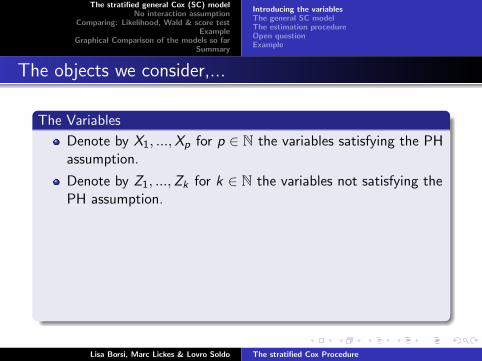
The objects we consider,...
The Variables
Denote by X1, ...,Xp for p ∈ N the variables satisfying the PHassumption.
Denote by Z1, ...,Zk for k ∈ N the variables not satisfying thePH assumption.
Define a single new variable Z ∗
1 Categorize each Zi
2 Form combinations of categories (strata)3 The strata are the categories of Z∗
k∗ denotes the number of combinations, i.e. Z ∗ has k∗
categories.
Lisa Borsi, Marc Lickes & Lovro Soldo The stratified Cox Procedure
The stratified general Cox (SC) modelNo interaction assumption
Comparing: Likelihood, Wald & score testExample
Graphical Comparison of the models so farSummary
Introducing the variablesThe general SC modelThe estimation procedureOpen questionExample
The objects we consider,...
The Variables
Denote by X1, ...,Xp for p ∈ N the variables satisfying the PHassumption.
Denote by Z1, ...,Zk for k ∈ N the variables not satisfying thePH assumption.
Define a single new variable Z ∗
1 Categorize each Zi
2 Form combinations of categories (strata)3 The strata are the categories of Z∗
k∗ denotes the number of combinations, i.e. Z ∗ has k∗
categories.
Lisa Borsi, Marc Lickes & Lovro Soldo The stratified Cox Procedure

The stratified general Cox (SC) modelNo interaction assumption
Comparing: Likelihood, Wald & score testExample
Graphical Comparison of the models so farSummary
Introducing the variablesThe general SC modelThe estimation procedureOpen questionExample
Illustrate this immediately with an example.
180 5. The Stratified Cox Procedure
EXAMPLE (continued)Adjusted Survival Curves for Rxfrom Stratified Cox Model(adjusted for log WBC)
1
0.8
0.6
0.4
0.2
00 8 16 24 32
Treatment, female
Treatment, malePlacebo, female
Placebo, male
Days
S
As mentioned above, adjusted survival curves canbe obtained for each stratum as shown here. Herewe have shown four survival curves because wewant to compare the survival for two treatmentgroups over each of two strata.
If we compare treatment and placebo group sepa-rately by sex, we can see that the treatment grouphas consistently better survival prognosis than theplacebo group for females and males separately.This supports our findings about the hazard ratiofor the treatment effect derived earlier from thecomputer results for the stratified Cox model.
III. The General StratifiedCox (SC) Model
In the previous example, we illustrated the SCmodel for one binary predictor not satisfying thePH assumption. We now describe the general formof the SC model that allows for stratification ofseveral predictors over several strata.
Example: one binary predictor!
General: several predictors, severalstrata
Z1, Z2, . . . , Zk, do not satisfy PHX1, X2, . . . , X p, satisfy PH
We assume that we have k variables not satisfyingthe PH assumption and p variables satisfying thePH assumption. The variables not satisfyingthe PH assumption we denote as Z1, Z2, . . . , Zk;the variables satisfying the PH assumption we de-note as X1, X2, . . . , X p.
Define a single new variable Z ":
1. categorize each Z i
2. form combinations of categories(strata)
3. the strata are the categories of Z "
To perform the stratified Cox procedure, we de-fine a single new variable, which we call Z ", fromthe Z’s to be used for stratification. We do this byforming categories of each Zi , including those Zithat are interval variables. We then form combi-nations of categories, and these combinations areour strata. These strata are the categories of thenew variable Z ".
EXAMPLEAge
Young Middle Old
Placebo
Treatment
Treatmentstatus
1 2 3
4 5 6
Z! = new variable with six categoriesStratify on Z!
For example, suppose k is 2, and the two Z’s areage (an interval variable) and treatment status(a binary variable). Then we categorize age into,say, three age groups—young, middle, and old. Wethen form six age group–by–treatment-status com-binations, as shown here. These six combinationsrepresent the different categories of a single newvariable that we stratify on in our stratified Coxmodel. We call this new variable Z ".
Lisa Borsi, Marc Lickes & Lovro Soldo The stratified Cox Procedure

The stratified general Cox (SC) modelNo interaction assumption
Comparing: Likelihood, Wald & score testExample
Graphical Comparison of the models so farSummary
Introducing the variablesThe general SC modelThe estimation procedureOpen questionExample
The model
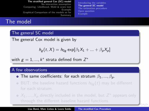
The general SC model
The general Cox model is given by
hg (t,X ) = h0g exp[β1X1 + ...+ βpXp]
with g = 1, ..., k∗ strata defined from Z ∗
A few observations
The same coefficients: for each stratum β1, ..., βp.
BUT: the baseline hazard functions h0g (t) may be differentfor each stratum.
X1, ...,Xp directly included in the model, but Z ∗ appears onlythrough the different baseline hazard functions.
Lisa Borsi, Marc Lickes & Lovro Soldo The stratified Cox Procedure
The stratified general Cox (SC) modelNo interaction assumption
Comparing: Likelihood, Wald & score testExample
Graphical Comparison of the models so farSummary
Introducing the variablesThe general SC modelThe estimation procedureOpen questionExample
The model
The general SC model
The general Cox model is given by
hg (t,X ) = h0g exp[β1X1 + ...+ βpXp]
with g = 1, ..., k∗ strata defined from Z ∗
A few observations
The same coefficients: for each stratum β1, ..., βp.
BUT: the baseline hazard functions h0g (t) may be differentfor each stratum.
X1, ...,Xp directly included in the model, but Z ∗ appears onlythrough the different baseline hazard functions.
Lisa Borsi, Marc Lickes & Lovro Soldo The stratified Cox Procedure

The stratified general Cox (SC) modelNo interaction assumption
Comparing: Likelihood, Wald & score testExample
Graphical Comparison of the models so farSummary
Introducing the variablesThe general SC modelThe estimation procedureOpen questionExample
How to obtain the regression coefficients β1, ...βp
The estimation procedure
1 We calculate the likelihood functions for each strataStrata: 1, . . . , k∗
Likelihood: L1, . . . , Lk∗
Hazard: h1, . . . , hk∗
2 We multiply all the likelihood function we have obtained thisway.
L = L1 × . . .× Lk∗
3 Estimate β by max likelihood of L(β).
Lisa Borsi, Marc Lickes & Lovro Soldo The stratified Cox Procedure

The stratified general Cox (SC) modelNo interaction assumption
Comparing: Likelihood, Wald & score testExample
Graphical Comparison of the models so farSummary
Introducing the variablesThe general SC modelThe estimation procedureOpen questionExample
Does the model really stand this ways?
Question:
One fundamental assumption is missing! Which one?
A hint: What do you know about the strata ?
Answer:
No interaction assumption between the strata and X1, ...,Xp ismissing. Otherwise the model would look differently. More to thislater.
Lisa Borsi, Marc Lickes & Lovro Soldo The stratified Cox Procedure

The stratified general Cox (SC) modelNo interaction assumption
Comparing: Likelihood, Wald & score testExample
Graphical Comparison of the models so farSummary
Introducing the variablesThe general SC modelThe estimation procedureOpen questionExample
Example: Leukemia data
Testing the PH assumption in R
Input:
> cox2 <- coxph(Surv(t,status) ~ logWBC + Rx + sex,
data=leuk, method="breslow")
> cox.zph(cox2)
Output:
rho chisq p
logWBC 0.0657 0.189 0.6638
Rx -0.1150 0.411 0.5214
sex -0.3656 3.839 0.0501
GLOBAL NA 3.969 0.2648
0.0501 ≈ 0.05⇒ PH assumption isviolated for SEX
Lisa Borsi, Marc Lickes & Lovro Soldo The stratified Cox Procedure

The stratified general Cox (SC) modelNo interaction assumption
Comparing: Likelihood, Wald & score testExample
Graphical Comparison of the models so farSummary
Introducing the variablesThe general SC modelThe estimation procedureOpen questionExample
Example: Leukemia data
PH assumptionnot satisfied forSEX
Lisa Borsi, Marc Lickes & Lovro Soldo The stratified Cox Procedure

The stratified general Cox (SC) modelNo interaction assumption
Comparing: Likelihood, Wald & score testExample
Graphical Comparison of the models so farSummary
Introducing the variablesThe general SC modelThe estimation procedureOpen questionExample
Example: Leukemia data
PH assumption not satisfied for SEX
use stratified Cox model
control for SEX by stratification
include logWBC and Rx in the model
hazard function for stratified Cox model:hg (t,X) = h0g (t)exp[β1 logWBC+β2Rx],g = 1 for females, g = 2 for males.
Lisa Borsi, Marc Lickes & Lovro Soldo The stratified Cox Procedure
The stratified general Cox (SC) modelNo interaction assumption
Comparing: Likelihood, Wald & score testExample
Graphical Comparison of the models so farSummary
Introducing the variablesThe general SC modelThe estimation procedureOpen questionExample
Example: Leukemia data
Input
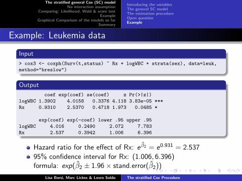
> cox3 <- coxph(Surv(t,status) ~ Rx + logWBC + strata(sex), data=leuk,
method="breslow")
Output
coef exp(coef) se(coef) z Pr(>|z|)
logWBC 1.3902 4.0158 0.3376 4.118 3.83e-05 ***
Rx 0.9310 2.5370 0.4718 1.973 0.0485 *
exp(coef) exp(-coef) lower .95 upper .95
logWBC 4.016 0.2490 2.072 7.783
Rx 2.537 0.3942 1.006 6.396
Hazard ratio for the effect of Rx: e β2 = e0.931 = 2.537
95% confidence interval for Rx: (1.006, 6.396)formula: exp(β2 ± 1.96× stand.error(β2))
Lisa Borsi, Marc Lickes & Lovro Soldo The stratified Cox Procedure

The stratified general Cox (SC) modelNo interaction assumption
Comparing: Likelihood, Wald & score testExample
Graphical Comparison of the models so farSummary
Introducing the variablesThe general SC modelThe estimation procedureOpen questionExample
Test significance of Rx adjusted for logWBC and SEX
R-output
> cox3$loglik[2]
[1] -57.55975
> cox4$loglik[2]
[1] -59.64846
> #Likelihood ratio statistic (significance of Rx)
> pchisq(-2*cox4$loglik[2]-(-2*cox3$loglik[2]), 1, lower.tail = FALSE)
[1] 0.040966
> cox3$coefficient[2]
0.9309646
> sqrt(diag(cox3$var))[2]
[1] 0.4717663
> pchisq((cox3$coefficient[2]/sqrt(diag(cox3$var))[2])^2, 1,
lower.tail = FALSE)
0.04845462
LR and Wald tests lead to same conclusions
Lisa Borsi, Marc Lickes & Lovro Soldo The stratified Cox Procedure

The stratified general Cox (SC) modelNo interaction assumption
Comparing: Likelihood, Wald & score testExample
Graphical Comparison of the models so farSummary
Introducing the variablesThe general SC modelThe estimation procedureOpen questionExample
Let’s have a closer look at the hazard functions
Stratified Cox model for females and males:
Females (g = 1): h1(t,X) = h01(t)exp[β1logWBC+β2Rx]
Males (g = 2): h2(t,X) = h02(t)exp[β1logWBC+β2Rx]
Note:
h01 and h02 are different ⇒ different survival curves forfemales and males
β1 and β2 are the same ⇒ same HR’s for females and males
(e β1 , e β2)
in this model: no interaction between variables in the modeland stratified variables
Lisa Borsi, Marc Lickes & Lovro Soldo The stratified Cox Procedure

The stratified general Cox (SC) modelNo interaction assumption
Comparing: Likelihood, Wald & score testExample
Graphical Comparison of the models so farSummary
Introducing the variablesThe general SC modelThe estimation procedureOpen questionExample
Example: Leukemia data
Lisa Borsi, Marc Lickes & Lovro Soldo The stratified Cox Procedure

The stratified general Cox (SC) modelNo interaction assumption
Comparing: Likelihood, Wald & score testExample
Graphical Comparison of the models so farSummary
The interaction modelEstimation procedure
No interaction assumption
No interaction assumption
Lisa Borsi, Marc Lickes & Lovro Soldo The stratified Cox Procedure

The stratified general Cox (SC) modelNo interaction assumption
Comparing: Likelihood, Wald & score testExample
Graphical Comparison of the models so farSummary
The interaction modelEstimation procedure
The interaction model
The interaction model
hg (t) = h0g (t) exp[β1gX1 + ...+ βpgXp] (1)
The difference to the no-interaction model is that the coefficientsβ depend on the strata.
An alternative interaction model
hg (t) = h0g (t)[β∗1X1 + ...+ β∗pXp +k∗−1∑j=1
p∑i=1
β∗ijXiZ∗j ] (2)
where the β∗ do not involve g .
Lisa Borsi, Marc Lickes & Lovro Soldo The stratified Cox Procedure

The stratified general Cox (SC) modelNo interaction assumption
Comparing: Likelihood, Wald & score testExample
Graphical Comparison of the models so farSummary
The interaction modelEstimation procedure
The interaction models
Claim
The formulations (1) and (2) are equivalent.
Proof.
See blackboard, we derive the equivalence for the previousexample.
Lisa Borsi, Marc Lickes & Lovro Soldo The stratified Cox Procedure

The stratified general Cox (SC) modelNo interaction assumption
Comparing: Likelihood, Wald & score testExample
Graphical Comparison of the models so farSummary
The interaction modelEstimation procedure
Likelihood ratio test
The test statistic is given by
LR = −2 ln LR − (−2 ln LF )
where LR denotes the no interaction model, and LF theinteraction model.
under H0 : no-interaction, we have that
LR ∼ χ2p(k∗−1)
Lisa Borsi, Marc Lickes & Lovro Soldo The stratified Cox Procedure

The stratified general Cox (SC) modelNo interaction assumption
Comparing: Likelihood, Wald & score testExample
Graphical Comparison of the models so farSummary
Assumptions and NotationsWho is . . . ?Definition of the different testsAn exampleComparing “intuitively”
Comparing: Likelihood, Wald & score test
Comparing: Likelihood, Wald & score test
Lisa Borsi, Marc Lickes & Lovro Soldo The stratified Cox Procedure

The stratified general Cox (SC) modelNo interaction assumption
Comparing: Likelihood, Wald & score testExample
Graphical Comparison of the models so farSummary
Assumptions and NotationsWho is . . . ?Definition of the different testsAn exampleComparing “intuitively”
Comparing Likelihood, Wald & Score Test
In this Section we will compare the following tests, which are allbased on Likelihood Theory.
1 Likelihood
2 Wald
3 Score
Lisa Borsi, Marc Lickes & Lovro Soldo The stratified Cox Procedure

The stratified general Cox (SC) modelNo interaction assumption
Comparing: Likelihood, Wald & score testExample
Graphical Comparison of the models so farSummary
Assumptions and NotationsWho is . . . ?Definition of the different testsAn exampleComparing “intuitively”
Assumptions and Notations:
As usual:
X denotes the data
θ = (θ1, . . . , θp) are the parameters we want to estimate.
L(θ,X ) will denote the likelihood or partial likelihood function.
We maximize the likelihood (or log-likelihood) with θ(X ) = θ.
H0 is θ = θ0.
Lisa Borsi, Marc Lickes & Lovro Soldo The stratified Cox Procedure

The stratified general Cox (SC) modelNo interaction assumption
Comparing: Likelihood, Wald & score testExample
Graphical Comparison of the models so farSummary
Assumptions and NotationsWho is . . . ?Definition of the different testsAn exampleComparing “intuitively”
The definition of the score vector
Fisher’s score vector U(θ).
The first derivative of the log-likelihood function is called (Fisher’s)score vector,
U(θ) =∂
∂θln L(θ,X )
Remember: the derivative w.r.t. a vector is a vector, with entries:
Ui (θ) = ∂∂θi
ln(L(θ,X )).
For U we haveEθ[U(θ)] = 0
At a maximum θ we have:
U(θ) = (0, . . . , 0)
Lisa Borsi, Marc Lickes & Lovro Soldo The stratified Cox Procedure

The stratified general Cox (SC) modelNo interaction assumption
Comparing: Likelihood, Wald & score testExample
Graphical Comparison of the models so farSummary
Assumptions and NotationsWho is . . . ?Definition of the different testsAn exampleComparing “intuitively”
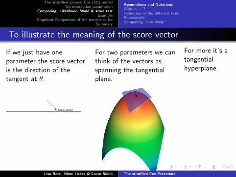
To illustrate the meaning of the score vector
If we just have oneparameter the score vectoris the direction of thetangent at θ.
Score vector
For two parameters we canthink of the vectors asspanning the tangentialplane.
For more it’s atangentialhyperplane.
Not so easy todraw, but Iguess you canimagine it! :)
Lisa Borsi, Marc Lickes & Lovro Soldo The stratified Cox Procedure

The stratified general Cox (SC) modelNo interaction assumption
Comparing: Likelihood, Wald & score testExample
Graphical Comparison of the models so farSummary
Assumptions and NotationsWho is . . . ?Definition of the different testsAn exampleComparing “intuitively”
To illustrate the meaning of the score vector
If we just have oneparameter the score vectoris the direction of thetangent at θ.
Score vector
For two parameters we canthink of the vectors asspanning the tangentialplane.
For more it’s atangentialhyperplane.
Not so easy todraw, but Iguess you canimagine it! :)
Lisa Borsi, Marc Lickes & Lovro Soldo The stratified Cox Procedure

The stratified general Cox (SC) modelNo interaction assumption
Comparing: Likelihood, Wald & score testExample
Graphical Comparison of the models so farSummary
Assumptions and NotationsWho is . . . ?Definition of the different testsAn exampleComparing “intuitively”
Covariance matrix
We can also look at the second momentum, this is called:
The Fisher information matrix i(θ).
The Fisher information matrix is a p × p matrix defined by:
i(θ) = Eθ
[U(θ)TU(θ)
]=
{−Eθ
[∂2
∂θi∂θjln L(θ,X )
]}i=1,...,pj=1,...,p
Mostly this is to hard to compute, thus we estimate i with:
i(θ) =: Ii ,j(θ) := − ∂2
∂θi∂θjln L(θ,X ), i = 1, . . . , p, j = 1, . . . , p
Lisa Borsi, Marc Lickes & Lovro Soldo The stratified Cox Procedure

The stratified general Cox (SC) modelNo interaction assumption
Comparing: Likelihood, Wald & score testExample
Graphical Comparison of the models so farSummary
Assumptions and NotationsWho is . . . ?Definition of the different testsAn exampleComparing “intuitively”
Who was Fisher?
Figure: R. A. Fisher(1890-1962)
One of the most important theoreticalbiologists, geneticists, evolutionarytheorists and statistician of the 20thCentury.
Founder of maximum likelihoodprinciple and variance statistics
Anders Hald about Fisher:a genius who almost
single-handedly created thefoundations for modernstatistical science
Lisa Borsi, Marc Lickes & Lovro Soldo The stratified Cox Procedure

The stratified general Cox (SC) modelNo interaction assumption
Comparing: Likelihood, Wald & score testExample
Graphical Comparison of the models so farSummary
Assumptions and NotationsWho is . . . ?Definition of the different testsAn exampleComparing “intuitively”
Who is Cox?
b.1924 Birmingham, England
1988: member of the Department ofStatistics at Oxford University
1990: won the Kettering Prize andGold Medal for Cancer Research for”the development of the ProportionalHazard Regression Model.”
1994 retired Figure: D. R. Cox(1924 - )
Lisa Borsi, Marc Lickes & Lovro Soldo The stratified Cox Procedure

The stratified general Cox (SC) modelNo interaction assumption
Comparing: Likelihood, Wald & score testExample
Graphical Comparison of the models so farSummary
Assumptions and NotationsWho is . . . ?Definition of the different testsAn exampleComparing “intuitively”
We are ready to compare the tests
We already know the likelihood ratio test statistic:
LR := −2(
ln L(θ0,X )− ln L(θ,X ))
The Wald test statistic is defined as:
W := (θ − θ0)T I (θ)(θ − θ0)
And the score test uses the Fisher score vector:
S := U(θ0)T I−1(θ0)U(θ0)
Note: They all converge to a χ2p distribution.
The advantage of score test: it does not depend on θ.
Lisa Borsi, Marc Lickes & Lovro Soldo The stratified Cox Procedure

The stratified general Cox (SC) modelNo interaction assumption
Comparing: Likelihood, Wald & score testExample
Graphical Comparison of the models so farSummary
Assumptions and NotationsWho is . . . ?Definition of the different testsAn exampleComparing “intuitively”
We are ready to compare the tests
We already know the likelihood ratio test statistic:
LR := −2(
ln L(θ0,X )− ln L(θ,X ))→ χ2
p
The Wald test statistic is defined as:
W := (θ − θ0)T I (θ)(θ − θ0)→ χ2p
And the score test uses the Fisher score vector:
S := U(θ0)T I−1(θ0)U(θ0)→ χ2p
Note: They all converge to a χ2p distribution.
The advantage of score test: it does not depend on θ.
Lisa Borsi, Marc Lickes & Lovro Soldo The stratified Cox Procedure

The stratified general Cox (SC) modelNo interaction assumption
Comparing: Likelihood, Wald & score testExample
Graphical Comparison of the models so farSummary
Assumptions and NotationsWho is . . . ?Definition of the different testsAn exampleComparing “intuitively”
Let’s look at an example
Given:
Censored sample of size n of exponentially dying populationwith hazard rate λ.
observed survival time of individual i is Ti with variable forfailure δi .
Test for null hypothesis: λ0 = 1.
The Likelihood function is given by:
L(λ, (Ti , δi )) =n∏
i=1
λδi e−λTi = λDe−λT
where T =∑n
i=1 Ti , is the total timeand D =
∑ni=1 δi is the observed number of deaths.
Lisa Borsi, Marc Lickes & Lovro Soldo The stratified Cox Procedure

The stratified general Cox (SC) modelNo interaction assumption
Comparing: Likelihood, Wald & score testExample
Graphical Comparison of the models so farSummary
Assumptions and NotationsWho is . . . ?Definition of the different testsAn exampleComparing “intuitively”
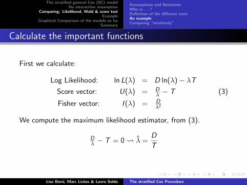
Calculate the important functions
First we calculate:
Log Likelihood: ln L(λ) = D ln(λ)− λTScore vector: U(λ) = d
dλ ln L(λ) = Dλ − T (3)
Fisher vector: I (λ) = − d2
dλ2ln L(λ) = D
λ2
We compute the maximum likelihood estimator, from (3).
Dλ − T = 0 λ =
D
T
Lisa Borsi, Marc Lickes & Lovro Soldo The stratified Cox Procedure
The stratified general Cox (SC) modelNo interaction assumption
Comparing: Likelihood, Wald & score testExample
Graphical Comparison of the models so farSummary
Assumptions and NotationsWho is . . . ?Definition of the different testsAn exampleComparing “intuitively”
Calculate the important functions
First we calculate:
Log Likelihood: ln L(λ) = D ln(λ)− λTScore vector: U(λ) = D
λ − T (3)
Fisher vector: I (λ) = Dλ2
We compute the maximum likelihood estimator, from (3).
Dλ − T = 0 λ =
D
T
Lisa Borsi, Marc Lickes & Lovro Soldo The stratified Cox Procedure

The stratified general Cox (SC) modelNo interaction assumption
Comparing: Likelihood, Wald & score testExample
Graphical Comparison of the models so farSummary
Assumptions and NotationsWho is . . . ?Definition of the different testsAn exampleComparing “intuitively”
Comparing the tests:
Likelihood ratio test:
LR = −2(
ln L(λ0,X )− ln L(λ,X ))
= −2((D ln(1)− 1 · T )−
(D ln(DT −
DT · S
))= 2
(T − D + D ln(DT )
)
Wald test:
W = (λ− λ0)T I (λ)(λ− λ0)
=(DT − 1
)D
(D/S)2
(DT − 1
)= (D−T )2
D
Score test:
S = U(λ0)T I−1(λ0)U(λ0)
=(DT − 1
)1D2
(DT − 1
)= (D−T )2
D
Lisa Borsi, Marc Lickes & Lovro Soldo The stratified Cox Procedure

The stratified general Cox (SC) modelNo interaction assumption
Comparing: Likelihood, Wald & score testExample
Graphical Comparison of the models so farSummary
Assumptions and NotationsWho is . . . ?Definition of the different testsAn exampleComparing “intuitively”
Comparing the tests:
Likelihood ratio test:
LR = −2(
ln L(λ0,X )− ln L(λ,X ))
= −2((D ln(1)− 1 · T )−
(D ln(DT −
DT · S
))= 2
(T − D + D ln(DT )
)Wald test:
W = (λ− λ0)T I (λ)(λ− λ0)
=(DT − 1
)D
(D/S)2
(DT − 1
)= (D−T )2
D
Score test:
S = U(λ0)T I−1(λ0)U(λ0)
=(DT − 1
)1D2
(DT − 1
)= (D−T )2
D
Lisa Borsi, Marc Lickes & Lovro Soldo The stratified Cox Procedure

The stratified general Cox (SC) modelNo interaction assumption
Comparing: Likelihood, Wald & score testExample
Graphical Comparison of the models so farSummary
Assumptions and NotationsWho is . . . ?Definition of the different testsAn exampleComparing “intuitively”
Comparing the tests “intuitively”.
Assume the plot of ln L(θ) against θ looks like this:
Lisa Borsi, Marc Lickes & Lovro Soldo The stratified Cox Procedure

The stratified general Cox (SC) modelNo interaction assumption
Comparing: Likelihood, Wald & score testExample
Graphical Comparison of the models so farSummary
Assumptions and NotationsWho is . . . ?Definition of the different testsAn exampleComparing “intuitively”
Comparing the tests “intuitively”.
What would be this value?
Lisa Borsi, Marc Lickes & Lovro Soldo The stratified Cox Procedure

The stratified general Cox (SC) modelNo interaction assumption
Comparing: Likelihood, Wald & score testExample
Graphical Comparison of the models so farSummary
Assumptions and NotationsWho is . . . ?Definition of the different testsAn exampleComparing “intuitively”
Comparing the tests “intuitively”.
Correct. It’s θ0.
Lisa Borsi, Marc Lickes & Lovro Soldo The stratified Cox Procedure

The stratified general Cox (SC) modelNo interaction assumption
Comparing: Likelihood, Wald & score testExample
Graphical Comparison of the models so farSummary
Assumptions and NotationsWho is . . . ?Definition of the different testsAn exampleComparing “intuitively”
Comparing the tests “intuitively”.
And what about this one?
Lisa Borsi, Marc Lickes & Lovro Soldo The stratified Cox Procedure

The stratified general Cox (SC) modelNo interaction assumption
Comparing: Likelihood, Wald & score testExample
Graphical Comparison of the models so farSummary
Assumptions and NotationsWho is . . . ?Definition of the different testsAn exampleComparing “intuitively”
Comparing the tests “intuitively”.
Correct. It’s θ. Maximizing ln L(θ).
Lisa Borsi, Marc Lickes & Lovro Soldo The stratified Cox Procedure

The stratified general Cox (SC) modelNo interaction assumption
Comparing: Likelihood, Wald & score testExample
Graphical Comparison of the models so farSummary
Assumptions and NotationsWho is . . . ?Definition of the different testsAn exampleComparing “intuitively”
Comparing the tests “intuitively”.
What would be this quantity?
Lisa Borsi, Marc Lickes & Lovro Soldo The stratified Cox Procedure

The stratified general Cox (SC) modelNo interaction assumption
Comparing: Likelihood, Wald & score testExample
Graphical Comparison of the models so farSummary
Assumptions and NotationsWho is . . . ?Definition of the different testsAn exampleComparing “intuitively”
Comparing the tests “intuitively”.
That’s the Likelihood ratio test. Comparing ln L(θ0) with ln L(θ).
LR test
Lisa Borsi, Marc Lickes & Lovro Soldo The stratified Cox Procedure

The stratified general Cox (SC) modelNo interaction assumption
Comparing: Likelihood, Wald & score testExample
Graphical Comparison of the models so farSummary
Assumptions and NotationsWho is . . . ?Definition of the different testsAn exampleComparing “intuitively”
Comparing the tests “intuitively”.
And this one?
LR test
Lisa Borsi, Marc Lickes & Lovro Soldo The stratified Cox Procedure

The stratified general Cox (SC) modelNo interaction assumption
Comparing: Likelihood, Wald & score testExample
Graphical Comparison of the models so farSummary
Assumptions and NotationsWho is . . . ?Definition of the different testsAn exampleComparing “intuitively”
Comparing the tests “intuitively”.
That’s it. The Wald test.
Wald test
LR test
Lisa Borsi, Marc Lickes & Lovro Soldo The stratified Cox Procedure

The stratified general Cox (SC) modelNo interaction assumption
Comparing: Likelihood, Wald & score testExample
Graphical Comparison of the models so farSummary
Assumptions and NotationsWho is . . . ?Definition of the different testsAn exampleComparing “intuitively”
Comparing the tests “intuitively”.
Where would be the score test?
Wald test
LR test
Lisa Borsi, Marc Lickes & Lovro Soldo The stratified Cox Procedure

The stratified general Cox (SC) modelNo interaction assumption
Comparing: Likelihood, Wald & score testExample
Graphical Comparison of the models so farSummary
Assumptions and NotationsWho is . . . ?Definition of the different testsAn exampleComparing “intuitively”
Comparing the tests “intuitively”.
Great.
Wald test
LR test
Score test
Lisa Borsi, Marc Lickes & Lovro Soldo The stratified Cox Procedure

The stratified general Cox (SC) modelNo interaction assumption
Comparing: Likelihood, Wald & score testExample
Graphical Comparison of the models so farSummary
Assumptions and NotationsWho is . . . ?Definition of the different testsAn exampleComparing “intuitively”
Comparing the tests “intuitively”.
Great. We see how the tests are “related” to the likelihoodfunction.
Wald test
LR test
Score test
Lisa Borsi, Marc Lickes & Lovro Soldo The stratified Cox Procedure

The stratified general Cox (SC) modelNo interaction assumption
Comparing: Likelihood, Wald & score testExample
Graphical Comparison of the models so farSummary
LayoutCheck PH assumptionStratifyInteraction?
Example
Example
Lisa Borsi, Marc Lickes & Lovro Soldo The stratified Cox Procedure

The stratified general Cox (SC) modelNo interaction assumption
Comparing: Likelihood, Wald & score testExample
Graphical Comparison of the models so farSummary
LayoutCheck PH assumptionStratifyInteraction?
Example involving several stratification variables
Data:
survival times in days for 137 lung cancer patients
exposure variable of interest: treatment status (standard=1,test=2)
control variables: cell type (4 types), performance status,disease duration, age, prior therapy status
How to proceed:
check PH assumption
stratify on the variables not satisfying PH assumption
check no-interaction assumption: fit interaction model andtest for significance
Lisa Borsi, Marc Lickes & Lovro Soldo The stratified Cox Procedure

The stratified general Cox (SC) modelNo interaction assumption
Comparing: Likelihood, Wald & score testExample
Graphical Comparison of the models so farSummary
LayoutCheck PH assumptionStratifyInteraction?
Example involving several stratification variables
188 5. The Stratified Cox Procedure
EXAMPLE (Remission Data)
Z! = sex , k! = 2, Z!
1 = sex(0,1), X1 = log WBC, X2 = Rx (p = 2) p(k! " 1) = 2, so LR ~ #2
2df under H0: no interaction .
Returning to the remission data example, forwhich p = 2 and k! = 2, the value of p(k! " 1)is equal to two times (2 " 1), which equals two.Thus, to test whether the SEX variable interactswith the log WBC and Rx predictors, the degreesof freedom for the LR statistic is two, as previouslydescribed.
V. A Second ExampleInvolving SeveralStratification Variables
The dataset “vets.dat” considers survival times indays for 137 patients from the Veteran’s Adminis-tration Lung Cancer Trial cited by Kalbfleisch andPrentice in their text (The Statistical Analysis ofSurvival Time Data, Wiley, pp. 223–224, 1980). Theexposure variable of interest is treatment status.Other variables of interest as control variables arecell type (four types, defined in terms of dummyvariables), performance status, disease duration,age, and prior therapy status. Failure status is de-fined by the status variable. A complete list of thevariables is shown here.
Here we provide computer output obtained fromfitting a Cox PH model to these data. Using theP(PH) information in the last column, we can seethat at least four of the variables listed have P(PH)values below the 0.100 level. These four variablesare labeled in the output as large cell (0.033),adeno cell (0.081), small cell (0.078), and Perf. Stat(0.000). Notice that the three variables, large cell,adeno cell, and small cell, are dummy variablesthat distinguish the four categories of cell type.
Thus, it appears from the P(PH) results that thevariables cell type (defined using dummy vari-ables) and performance status do not satisfy thePH assumption.
Based on the conclusions just made about the PHassumption, we now describe a stratified Cox anal-ysis that stratifies on the variables, cell type andperformance status.
EXAMPLE vets.dat: survival time in days, n = 137
Veteran’s Administration Lung Cancer Trial Column 1: Treatment (standard = 1, test = 2) Column 2: Cell type 1 (large = 1, other = 0) Column 3: Cell type 2 (adeno = 1, other = 0) Column 4: Cell type 3 (small = 1, other = 0) Column 5: Cell type 4 (squamous = 1, other = 0)Column 6: Survival time (days) Column 7: Performance status (0 = worst, ...,
100 = best) Column 8: Disease duration (months) Column 9: Age Column 10: Prior therapy (none = 0, some = 10) Column 11: Status (0 = censored, 1 = died)
Cox regression Analysis time _t: survt
Coef.Std.Err. p > |z|
Haz.Ratio
[95% Conf. Interval] P(PH)
Treatment 0.290 0.207 0.162 1.336 0.890 2.006 0.628Large cell 0.400 0.283 0.157 1.491 0.857 2.594 0.033Adeno cell 1.188 0.301 0.000 3.281 1.820 5.915 0.081Small cell 0.856 0.275 0.002 2.355 1.374 4.037 0.078Perf. Stat –0.033 0.006 0.000 0.968 0.958 0.978 0.000Dis. Durat. 0.000 0.009 0.992 1.000 0.982 1.018 0.919Age –0.009 0.009 0.358 0.991 0.974 1.010 0.198Pr. Therapy 0.007 0.023 0.755 1.007 0.962 1.054 0.145
No. of subjects = 137 Log likelihood = –475.180
Variables not satisfying PH: • cell type (3 dummy variables) • performance status • prior therapy (possibly)
SC model: stratifies on cell type and per-formance status
cell type and performance status do not verify PH assumption
use stratified Cox model: stratify on cell type and perf stat
Lisa Borsi, Marc Lickes & Lovro Soldo The stratified Cox Procedure

The stratified general Cox (SC) modelNo interaction assumption
Comparing: Likelihood, Wald & score testExample
Graphical Comparison of the models so farSummary
LayoutCheck PH assumptionStratifyInteraction?
Example involving several stratification variables
stratified Cox analysis:
stratify on 2 variables: cell type and performance status
new categorical variable Z ∗
categories of Z ∗ = all possible combinations of categories ofcell type and performance status
cell type: 4 categories
performance status ∈ (0, 100), but need categorical variable
⇒ new variable PSbin =
{1 if performance ≥ 60,
0 otherwise.
Z ∗ has k∗ = 4× 2 = 8 categories
Lisa Borsi, Marc Lickes & Lovro Soldo The stratified Cox Procedure

The stratified general Cox (SC) modelNo interaction assumption
Comparing: Likelihood, Wald & score testExample
Graphical Comparison of the models so farSummary
LayoutCheck PH assumptionStratifyInteraction?
Example involving several stratification variables
Stratified Cox analysis in R:
Input
cox_3 <- coxph(Surv(time,status) ~ treatment + age +
strata(large_cell,small_cell,adeno_cell,PSbin),
data=vets, method="breslow")
summary(cox_3)
Output
coef exp(coef) se(coef) z Pr(>|z|)
treatment 0.125398 1.133599 0.208471 0.602 0.547
age -0.001307 0.998694 0.010103 -0.129 0.897
exp(coef) exp(-coef) lower .95 upper .95
treatment 1.1336 0.8821 0.7534 1.706
age 0.9987 1.0013 0.9791 1.019
Lisa Borsi, Marc Lickes & Lovro Soldo The stratified Cox Procedure

The stratified general Cox (SC) modelNo interaction assumption
Comparing: Likelihood, Wald & score testExample
Graphical Comparison of the models so farSummary
LayoutCheck PH assumptionStratifyInteraction?
Example involving several stratification variables
No-interaction model
hg (t,X) = h0g (t)exp[β1Treatment+β2Age], g = 1, 2, . . . , 8
Is an interaction model appropriate?
define an interaction model
test H0= no-interaction model is acceptable by LR test
Lisa Borsi, Marc Lickes & Lovro Soldo The stratified Cox Procedure

The stratified general Cox (SC) modelNo interaction assumption
Comparing: Likelihood, Wald & score testExample
Graphical Comparison of the models so farSummary
LayoutCheck PH assumptionStratifyInteraction?
Example: interaction model
Hazard function for interaction model:
hg (t,X) = h0g (t)exp[β1Treatment + β2Age
+β11(Z ∗1 × Treatment) + · · ·+ β17(Z ∗
7 × Treatment)
+β21(Z ∗1 × Age) + · · ·+ β27(Z ∗
7 × Age)]
where Z ∗1 = large cell, Z ∗
2 = small cell, Z ∗3 = adeno cell,
Z ∗4 = PSbin, Z ∗
5 = Z ∗1 × Z ∗
4 , Z ∗6 = Z ∗
2 × Z ∗4 and Z ∗
7 = Z ∗3 × Z ∗
4
Lisa Borsi, Marc Lickes & Lovro Soldo The stratified Cox Procedure

The stratified general Cox (SC) modelNo interaction assumption
Comparing: Likelihood, Wald & score testExample
Graphical Comparison of the models so farSummary
LayoutCheck PH assumptionStratifyInteraction?
Example: interaction model
Input
cox_4 <- coxph(Surv(time,status) ~
treatment*strata(large_cell,small_cell,adeno_cell,PSbin)+
age*strata(large_cell,small_cell,adeno_cell,PSbin),
data=vets, method="breslow")
Lisa Borsi, Marc Lickes & Lovro Soldo The stratified Cox Procedure

The stratified general Cox (SC) modelNo interaction assumption
Comparing: Likelihood, Wald & score testExample
Graphical Comparison of the models so farSummary
LayoutCheck PH assumptionStratifyInteraction?
Test for significance of the interaction model
Likelihood ratio (LR) test
H0: no-interaction model acceptable,i.e. β’s of interaction terms are all zero
LR = −2(LRR − LRF )R = no-interaction model, F = interaction model
LR ∼ χ214 (14 coefficients of interaction terms)
if H0 rejected then interaction model is appropriate
Lisa Borsi, Marc Lickes & Lovro Soldo The stratified Cox Procedure

The stratified general Cox (SC) modelNo interaction assumption
Comparing: Likelihood, Wald & score testExample
Graphical Comparison of the models so farSummary
LayoutCheck PH assumptionStratifyInteraction?
Test for significance of the interaction model
Likelihood ratio test in R:
> red$loglik[2]
[1] -262.0195
> full$loglik[2]
[1] -249.972
> pchisq(-2*(red$loglik[2]-full$loglik[2]), 14, lower.tail=FALSE)
[1] 0.04462534
⇒ no-interaction assumption is rejected at 5% levelso interaction model is preferred
Lisa Borsi, Marc Lickes & Lovro Soldo The stratified Cox Procedure

The stratified general Cox (SC) modelNo interaction assumption
Comparing: Likelihood, Wald & score testExample
Graphical Comparison of the models so farSummary
Graphical Comparison of the models so far
Graphical Comparison of the models so far
Lisa Borsi, Marc Lickes & Lovro Soldo The stratified Cox Procedure
The stratified general Cox (SC) modelNo interaction assumption
Comparing: Likelihood, Wald & score testExample
Graphical Comparison of the models so farSummary
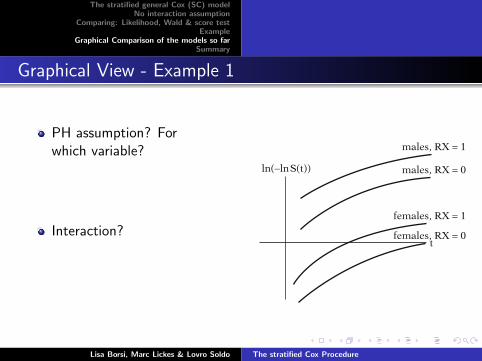
Graphical View - Example 1
PH assumption? Forwhich variable?
- PH for both RX and SEX,we see that since thecurves are parallel.
Interaction?
- No interaction, becausethey have the samedistance.
VI. A Graphical View of the Stratified Cox Approach 193
EXAMPLE (continued)
LR~!214df under H0: no interaction
LR = ("2 # –262.020) " ("2 # –249.972)= 524.040 " 499.944 = 24.096
P = 0.045 (significant at 0.05)Conclusion:Reject H0: interaction model ispreferred.
Might use further testing to simplifyinteraction model, e.g., test for sevenproducts involving treatment or test forseven products involving age.
.Thus, under the null hypothesis, the LR statisticis approximately chi-square with 14 degrees offreedom.
The computer results for the no-interaction andinteraction models give log-likelihood values of524.040 and 499.944, respectively. The differenceis 24.096. A chi-square value of 24.096 with 14 de-grees of freedom yields a p-value of 0.045, so thatthe test gives a significant result at the 0.05 level.This indicates that the no-interaction model is notacceptable and the interaction model is preferred.
Note, however, that it may be possible from fur-ther statistical testing to simplify the interactionmodel to have fewer than 14 product terms. Forexample, one might test for only the seven prod-uct terms involving treatment or only the sevenproduct terms involving age.
VI. A Graphical View of theStratified Cox Approach
a. h(t) = h0(t)exp(β1RX+β2SEX)
ln(! ln S(t)) = ln(! ln S0(t))+β1RX + β2SEX
ln(!lnS(t))
males, RX = 1
males, RX = 0
females, RX = 0
females, RX = 1
t
In this section we examine four log–log survivalplots illustrating the assumptions underlying astratified Cox model with or without interaction.Each of the four models considers two dichoto-mous predictors: treatment (coded RX = 1 forplacebo and RX = 0 for new treatment) and SEX(coded 0 for females and 1 for males). The fourmodels are as follows (see left).
a. h0(t)exp(β1RX + β2SEX). This modelassumes the PH assumption for both RXand SEX and also assumes no interactionbetween RX and SEX. Notice all fourlog–log curves are parallel (PH assumption)and the effect of treatment is the same forfemales and males (no interaction). Theeffect of treatment (controlling for SEX)can be interpreted as the distance betweenthe log–log curves from RX = 1 to RX = 0,for males and for females, separately.
Lisa Borsi, Marc Lickes & Lovro Soldo The stratified Cox Procedure

The stratified general Cox (SC) modelNo interaction assumption
Comparing: Likelihood, Wald & score testExample
Graphical Comparison of the models so farSummary
Graphical View - Example 1
PH assumption? Forwhich variable?
- PH for both RX and SEX,we see that since thecurves are parallel.
Interaction?
- No interaction, becausethey have the samedistance.
VI. A Graphical View of the Stratified Cox Approach 193
EXAMPLE (continued)
LR~!214df under H0: no interaction
LR = ("2 # –262.020) " ("2 # –249.972)= 524.040 " 499.944 = 24.096
P = 0.045 (significant at 0.05)Conclusion:Reject H0: interaction model ispreferred.
Might use further testing to simplifyinteraction model, e.g., test for sevenproducts involving treatment or test forseven products involving age.
.Thus, under the null hypothesis, the LR statisticis approximately chi-square with 14 degrees offreedom.
The computer results for the no-interaction andinteraction models give log-likelihood values of524.040 and 499.944, respectively. The differenceis 24.096. A chi-square value of 24.096 with 14 de-grees of freedom yields a p-value of 0.045, so thatthe test gives a significant result at the 0.05 level.This indicates that the no-interaction model is notacceptable and the interaction model is preferred.
Note, however, that it may be possible from fur-ther statistical testing to simplify the interactionmodel to have fewer than 14 product terms. Forexample, one might test for only the seven prod-uct terms involving treatment or only the sevenproduct terms involving age.
VI. A Graphical View of theStratified Cox Approach
a. h(t) = h0(t)exp(β1RX+β2SEX)
ln(! ln S(t)) = ln(! ln S0(t))+β1RX + β2SEX
ln(!lnS(t))
males, RX = 1
males, RX = 0
females, RX = 0
females, RX = 1
t
In this section we examine four log–log survivalplots illustrating the assumptions underlying astratified Cox model with or without interaction.Each of the four models considers two dichoto-mous predictors: treatment (coded RX = 1 forplacebo and RX = 0 for new treatment) and SEX(coded 0 for females and 1 for males). The fourmodels are as follows (see left).
a. h0(t)exp(β1RX + β2SEX). This modelassumes the PH assumption for both RXand SEX and also assumes no interactionbetween RX and SEX. Notice all fourlog–log curves are parallel (PH assumption)and the effect of treatment is the same forfemales and males (no interaction). Theeffect of treatment (controlling for SEX)can be interpreted as the distance betweenthe log–log curves from RX = 1 to RX = 0,for males and for females, separately.
h0(t)eβ1RX+β2SEX
Lisa Borsi, Marc Lickes & Lovro Soldo The stratified Cox Procedure

The stratified general Cox (SC) modelNo interaction assumption
Comparing: Likelihood, Wald & score testExample
Graphical Comparison of the models so farSummary
Graphical View - Example 1
PH assumption? Forwhich variable?
- PH for both RX and SEX,we see that since thecurves are parallel.
Interaction?
- No interaction, becausethey have the samedistance.
VI. A Graphical View of the Stratified Cox Approach 193
EXAMPLE (continued)
LR~!214df under H0: no interaction
LR = ("2 # –262.020) " ("2 # –249.972)= 524.040 " 499.944 = 24.096
P = 0.045 (significant at 0.05)Conclusion:Reject H0: interaction model ispreferred.
Might use further testing to simplifyinteraction model, e.g., test for sevenproducts involving treatment or test forseven products involving age.
.Thus, under the null hypothesis, the LR statisticis approximately chi-square with 14 degrees offreedom.
The computer results for the no-interaction andinteraction models give log-likelihood values of524.040 and 499.944, respectively. The differenceis 24.096. A chi-square value of 24.096 with 14 de-grees of freedom yields a p-value of 0.045, so thatthe test gives a significant result at the 0.05 level.This indicates that the no-interaction model is notacceptable and the interaction model is preferred.
Note, however, that it may be possible from fur-ther statistical testing to simplify the interactionmodel to have fewer than 14 product terms. Forexample, one might test for only the seven prod-uct terms involving treatment or only the sevenproduct terms involving age.
VI. A Graphical View of theStratified Cox Approach
a. h(t) = h0(t)exp(β1RX+β2SEX)
ln(! ln S(t)) = ln(! ln S0(t))+β1RX + β2SEX
ln(!lnS(t))
males, RX = 1
males, RX = 0
females, RX = 0
females, RX = 1
t
In this section we examine four log–log survivalplots illustrating the assumptions underlying astratified Cox model with or without interaction.Each of the four models considers two dichoto-mous predictors: treatment (coded RX = 1 forplacebo and RX = 0 for new treatment) and SEX(coded 0 for females and 1 for males). The fourmodels are as follows (see left).
a. h0(t)exp(β1RX + β2SEX). This modelassumes the PH assumption for both RXand SEX and also assumes no interactionbetween RX and SEX. Notice all fourlog–log curves are parallel (PH assumption)and the effect of treatment is the same forfemales and males (no interaction). Theeffect of treatment (controlling for SEX)can be interpreted as the distance betweenthe log–log curves from RX = 1 to RX = 0,for males and for females, separately.
Lisa Borsi, Marc Lickes & Lovro Soldo The stratified Cox Procedure

The stratified general Cox (SC) modelNo interaction assumption
Comparing: Likelihood, Wald & score testExample
Graphical Comparison of the models so farSummary
Graphical View - Example 2
PH assumption? Forwhich variable?
- PH for both RX and SEX(parallel)
Interaction?
- Between treatment andSEX
- Effect for the treatment islarger for males thenfemales. Bigger distancebetween RX=1 to RX=0.
194 5. The Stratified Cox Procedure
b. h(t) = h0(t) exp(β1RX + β2SEX+β3 RX ! SEX)
ln("ln S(t)) = ln("ln S0(t))+ β1RX+β2SEX+β3RX!SEX
ln(!lnS(t))
males, RX = 1
males, RX = 0
females, RX = 0females, RX = 1
t
c. h(t) = h0g(t)exp(β1RX)(g = 1 for males, g = 0 forfemales)ln("lnS(t)) = ln(" ln S0g(t))
+ β1RX
ln(!lnS(t))
males, RX = 1males, RX = 0
females, RX = 0
females, RX = 1t
d. h(t) = h0g(t)exp(β1RX+ β2 RX ! SEX)
(g = 1 for males, g = 0 forfemales)ln("ln S(t)) = ln("ln S0g(t))
+β1RX + β2 RX !SEX
ln(!lnS(t))
males, RX = 1
males, RX = 0
females, RX = 0females, RX = 1
t
b. h(t) = h0(t)exp(β1RX + β2SEX + β3RX ! SEX). This model assumes the PHassumption for both RX and SEX andallows for interaction between these twovariables. All four log–log curves areparallel (PH assumption) but the effect oftreatment is larger for males than femalesas the distance from RX = 1 to RX = 0 isgreater for males.
c. h(t) = h0g(t)exp(β1RX), where g = 1 formales, g = 0 for females. This is a stratifiedCox model in which the PH assumption isnot assumed for SEX. Notice the curves formales and females are not parallel.However, the curves for RX are parallelwithin each stratum of SEX indicating thatthe PH assumption is satisfied for RX. Thedistance between the log–log curves fromRX = 1 to RX = 0 is the same for malesand females indicating no interactionbetween RX and SEX.
d. h(t) = h0g(t) exp(β1RX + β2RX ! SEX),where g = 1 for males, g = 0 for females.This is a stratified Cox model allowing forinteraction of RX and SEX. The curves formales and females are not parallelalthough the PH assumption is satisfied forRX within each stratum of SEX. Thedistance between the log–log curves fromRX = 1 to RX = 0 is greater for males thanfemales indicating interaction between RXand SEX.
h0(t)eβ1RX+β2SEX+β3RX×SEX
Lisa Borsi, Marc Lickes & Lovro Soldo The stratified Cox Procedure

The stratified general Cox (SC) modelNo interaction assumption
Comparing: Likelihood, Wald & score testExample
Graphical Comparison of the models so farSummary
Graphical View - Example 3
PH assumption?
- PH assumption for RX.Stratified, for SEX.
- Notice the strata are nolonger parallel.
Interaction?
- Distance between RX=1and RX=0 is the sameindicating no interactionbetween RX and SEX.
194 5. The Stratified Cox Procedure
b. h(t) = h0(t) exp(β1RX + β2SEX+β3 RX ! SEX)
ln("ln S(t)) = ln("ln S0(t))+ β1RX+β2SEX+β3RX!SEX
ln(!lnS(t))
males, RX = 1
males, RX = 0
females, RX = 0females, RX = 1
t
c. h(t) = h0g(t)exp(β1RX)(g = 1 for males, g = 0 forfemales)ln("lnS(t)) = ln(" ln S0g(t))
+ β1RX
ln(!lnS(t))
males, RX = 1males, RX = 0
females, RX = 0
females, RX = 1t
d. h(t) = h0g(t)exp(β1RX+ β2 RX ! SEX)
(g = 1 for males, g = 0 forfemales)ln("ln S(t)) = ln("ln S0g(t))
+β1RX + β2 RX !SEX
ln(!lnS(t))
males, RX = 1
males, RX = 0
females, RX = 0females, RX = 1
t
b. h(t) = h0(t)exp(β1RX + β2SEX + β3RX ! SEX). This model assumes the PHassumption for both RX and SEX andallows for interaction between these twovariables. All four log–log curves areparallel (PH assumption) but the effect oftreatment is larger for males than femalesas the distance from RX = 1 to RX = 0 isgreater for males.
c. h(t) = h0g(t)exp(β1RX), where g = 1 formales, g = 0 for females. This is a stratifiedCox model in which the PH assumption isnot assumed for SEX. Notice the curves formales and females are not parallel.However, the curves for RX are parallelwithin each stratum of SEX indicating thatthe PH assumption is satisfied for RX. Thedistance between the log–log curves fromRX = 1 to RX = 0 is the same for malesand females indicating no interactionbetween RX and SEX.
d. h(t) = h0g(t) exp(β1RX + β2RX ! SEX),where g = 1 for males, g = 0 for females.This is a stratified Cox model allowing forinteraction of RX and SEX. The curves formales and females are not parallelalthough the PH assumption is satisfied forRX within each stratum of SEX. Thedistance between the log–log curves fromRX = 1 to RX = 0 is greater for males thanfemales indicating interaction between RXand SEX.
h00(t)eβ1RX ,
h01(t)eβ1RX
Lisa Borsi, Marc Lickes & Lovro Soldo The stratified Cox Procedure

The stratified general Cox (SC) modelNo interaction assumption
Comparing: Likelihood, Wald & score testExample
Graphical Comparison of the models so farSummary
Graphical View - Example 4
PH assumption?
- PH assumption for RX.Stratified, for SEX.
Interaction?
- Interaction between RXand SEX, bigger distancefor RX=1 and RX=0.
194 5. The Stratified Cox Procedure
b. h(t) = h0(t) exp(β1RX + β2SEX+β3 RX ! SEX)
ln("ln S(t)) = ln("ln S0(t))+ β1RX+β2SEX+β3RX!SEX
ln(!lnS(t))
males, RX = 1
males, RX = 0
females, RX = 0females, RX = 1
t
c. h(t) = h0g(t)exp(β1RX)(g = 1 for males, g = 0 forfemales)ln("lnS(t)) = ln(" ln S0g(t))
+ β1RX
ln(!lnS(t))
males, RX = 1males, RX = 0
females, RX = 0
females, RX = 1t
d. h(t) = h0g(t)exp(β1RX+ β2 RX ! SEX)
(g = 1 for males, g = 0 forfemales)ln("ln S(t)) = ln("ln S0g(t))
+β1RX + β2 RX !SEX
ln(!lnS(t))
males, RX = 1
males, RX = 0
females, RX = 0females, RX = 1
t
b. h(t) = h0(t)exp(β1RX + β2SEX + β3RX ! SEX). This model assumes the PHassumption for both RX and SEX andallows for interaction between these twovariables. All four log–log curves areparallel (PH assumption) but the effect oftreatment is larger for males than femalesas the distance from RX = 1 to RX = 0 isgreater for males.
c. h(t) = h0g(t)exp(β1RX), where g = 1 formales, g = 0 for females. This is a stratifiedCox model in which the PH assumption isnot assumed for SEX. Notice the curves formales and females are not parallel.However, the curves for RX are parallelwithin each stratum of SEX indicating thatthe PH assumption is satisfied for RX. Thedistance between the log–log curves fromRX = 1 to RX = 0 is the same for malesand females indicating no interactionbetween RX and SEX.
d. h(t) = h0g(t) exp(β1RX + β2RX ! SEX),where g = 1 for males, g = 0 for females.This is a stratified Cox model allowing forinteraction of RX and SEX. The curves formales and females are not parallelalthough the PH assumption is satisfied forRX within each stratum of SEX. Thedistance between the log–log curves fromRX = 1 to RX = 0 is greater for males thanfemales indicating interaction between RXand SEX.
h00(t)eβ1RX+β2RX×SEX ,
h01(t)eβ1RX+β2RX×SEX
Lisa Borsi, Marc Lickes & Lovro Soldo The stratified Cox Procedure

The stratified general Cox (SC) modelNo interaction assumption
Comparing: Likelihood, Wald & score testExample
Graphical Comparison of the models so farSummary
Overview of the examples
No interaction Interaction
PH Assumption
VI. A Graphical View of the Stratified Cox Approach 193
EXAMPLE (continued)
LR~!214df under H0: no interaction
LR = ("2 # –262.020) " ("2 # –249.972)= 524.040 " 499.944 = 24.096
P = 0.045 (significant at 0.05)Conclusion:Reject H0: interaction model ispreferred.
Might use further testing to simplifyinteraction model, e.g., test for sevenproducts involving treatment or test forseven products involving age.
.Thus, under the null hypothesis, the LR statisticis approximately chi-square with 14 degrees offreedom.
The computer results for the no-interaction andinteraction models give log-likelihood values of524.040 and 499.944, respectively. The differenceis 24.096. A chi-square value of 24.096 with 14 de-grees of freedom yields a p-value of 0.045, so thatthe test gives a significant result at the 0.05 level.This indicates that the no-interaction model is notacceptable and the interaction model is preferred.
Note, however, that it may be possible from fur-ther statistical testing to simplify the interactionmodel to have fewer than 14 product terms. Forexample, one might test for only the seven prod-uct terms involving treatment or only the sevenproduct terms involving age.
VI. A Graphical View of theStratified Cox Approach
a. h(t) = h0(t)exp(β1RX+β2SEX)
ln(! ln S(t)) = ln(! ln S0(t))+β1RX + β2SEX
ln(!lnS(t))
males, RX = 1
males, RX = 0
females, RX = 0
females, RX = 1
t
In this section we examine four log–log survivalplots illustrating the assumptions underlying astratified Cox model with or without interaction.Each of the four models considers two dichoto-mous predictors: treatment (coded RX = 1 forplacebo and RX = 0 for new treatment) and SEX(coded 0 for females and 1 for males). The fourmodels are as follows (see left).
a. h0(t)exp(β1RX + β2SEX). This modelassumes the PH assumption for both RXand SEX and also assumes no interactionbetween RX and SEX. Notice all fourlog–log curves are parallel (PH assumption)and the effect of treatment is the same forfemales and males (no interaction). Theeffect of treatment (controlling for SEX)can be interpreted as the distance betweenthe log–log curves from RX = 1 to RX = 0,for males and for females, separately.
194 5. The Stratified Cox Procedure
b. h(t) = h0(t) exp(β1RX + β2SEX+β3 RX ! SEX)
ln("ln S(t)) = ln("ln S0(t))+ β1RX+β2SEX+β3RX!SEX
ln(!lnS(t))
males, RX = 1
males, RX = 0
females, RX = 0females, RX = 1
t
c. h(t) = h0g(t)exp(β1RX)(g = 1 for males, g = 0 forfemales)ln("lnS(t)) = ln(" ln S0g(t))
+ β1RX
ln(!lnS(t))
males, RX = 1males, RX = 0
females, RX = 0
females, RX = 1t
d. h(t) = h0g(t)exp(β1RX+ β2 RX ! SEX)
(g = 1 for males, g = 0 forfemales)ln("ln S(t)) = ln("ln S0g(t))
+β1RX + β2 RX !SEX
ln(!lnS(t))
males, RX = 1
males, RX = 0
females, RX = 0females, RX = 1
t
b. h(t) = h0(t)exp(β1RX + β2SEX + β3RX ! SEX). This model assumes the PHassumption for both RX and SEX andallows for interaction between these twovariables. All four log–log curves areparallel (PH assumption) but the effect oftreatment is larger for males than femalesas the distance from RX = 1 to RX = 0 isgreater for males.
c. h(t) = h0g(t)exp(β1RX), where g = 1 formales, g = 0 for females. This is a stratifiedCox model in which the PH assumption isnot assumed for SEX. Notice the curves formales and females are not parallel.However, the curves for RX are parallelwithin each stratum of SEX indicating thatthe PH assumption is satisfied for RX. Thedistance between the log–log curves fromRX = 1 to RX = 0 is the same for malesand females indicating no interactionbetween RX and SEX.
d. h(t) = h0g(t) exp(β1RX + β2RX ! SEX),where g = 1 for males, g = 0 for females.This is a stratified Cox model allowing forinteraction of RX and SEX. The curves formales and females are not parallelalthough the PH assumption is satisfied forRX within each stratum of SEX. Thedistance between the log–log curves fromRX = 1 to RX = 0 is greater for males thanfemales indicating interaction between RXand SEX.
Stratified by SEX
194 5. The Stratified Cox Procedure
b. h(t) = h0(t) exp(β1RX + β2SEX+β3 RX ! SEX)
ln("ln S(t)) = ln("ln S0(t))+ β1RX+β2SEX+β3RX!SEX
ln(!lnS(t))
males, RX = 1
males, RX = 0
females, RX = 0females, RX = 1
t
c. h(t) = h0g(t)exp(β1RX)(g = 1 for males, g = 0 forfemales)ln("lnS(t)) = ln(" ln S0g(t))
+ β1RX
ln(!lnS(t))
males, RX = 1males, RX = 0
females, RX = 0
females, RX = 1t
d. h(t) = h0g(t)exp(β1RX+ β2 RX ! SEX)
(g = 1 for males, g = 0 forfemales)ln("ln S(t)) = ln("ln S0g(t))
+β1RX + β2 RX !SEX
ln(!lnS(t))
males, RX = 1
males, RX = 0
females, RX = 0females, RX = 1
t
b. h(t) = h0(t)exp(β1RX + β2SEX + β3RX ! SEX). This model assumes the PHassumption for both RX and SEX andallows for interaction between these twovariables. All four log–log curves areparallel (PH assumption) but the effect oftreatment is larger for males than femalesas the distance from RX = 1 to RX = 0 isgreater for males.
c. h(t) = h0g(t)exp(β1RX), where g = 1 formales, g = 0 for females. This is a stratifiedCox model in which the PH assumption isnot assumed for SEX. Notice the curves formales and females are not parallel.However, the curves for RX are parallelwithin each stratum of SEX indicating thatthe PH assumption is satisfied for RX. Thedistance between the log–log curves fromRX = 1 to RX = 0 is the same for malesand females indicating no interactionbetween RX and SEX.
d. h(t) = h0g(t) exp(β1RX + β2RX ! SEX),where g = 1 for males, g = 0 for females.This is a stratified Cox model allowing forinteraction of RX and SEX. The curves formales and females are not parallelalthough the PH assumption is satisfied forRX within each stratum of SEX. Thedistance between the log–log curves fromRX = 1 to RX = 0 is greater for males thanfemales indicating interaction between RXand SEX.
Lisa Borsi, Marc Lickes & Lovro Soldo The stratified Cox Procedure

The stratified general Cox (SC) modelNo interaction assumption
Comparing: Likelihood, Wald & score testExample
Graphical Comparison of the models so farSummary
The stratified general cox modelNo interaction assumptionComparing: Likelihood, Wald and score testGraphical Comparison of the models so far
Summary
Summary
Lisa Borsi, Marc Lickes & Lovro Soldo The stratified Cox Procedure

The stratified general Cox (SC) modelNo interaction assumption
Comparing: Likelihood, Wald & score testExample
Graphical Comparison of the models so farSummary
The stratified general cox modelNo interaction assumptionComparing: Likelihood, Wald and score testGraphical Comparison of the models so far
Summary
1 The stratified general Cox (SC) modelWhat to do if some variables do not satisfy the PHassumption?
⇒ Put them into stratas - general SC model:
hg (t,X ) = h0g exp[β1X1 + ...+ βpXp]
2 No interaction assumption- Same βi for each strata.
What if the βi ’s are different for each strata?⇒ Test the no-interaction model against the full (interaction)
model:
hg (t) = hg0(t)[β∗1X1 + ...+ β∗
pXp +k∗−1∑j=1
p∑i=1
β∗ijXiZ
∗j ]
(using log-likelihood, Wald or score test).
Lisa Borsi, Marc Lickes & Lovro Soldo The stratified Cox Procedure
The stratified general Cox (SC) modelNo interaction assumption
Comparing: Likelihood, Wald & score testExample
Graphical Comparison of the models so farSummary
The stratified general cox modelNo interaction assumptionComparing: Likelihood, Wald and score testGraphical Comparison of the models so far
Summary
3 Comparing: Likelihood, Wald & score testWhat are LR, Wald & score test?
⇒ Definitions:
LR := −2(
ln L(θ0,X )− ln L(θ,X ))→ χ2
p
W := (θ − θ0)T I (θ)(θ − θ0)→ χ2p
S := U(θ0)T I−1(θ0)U(θ0)→ χ2p
How are they “related” ?
Wald test
LR test
Score test
Lisa Borsi, Marc Lickes & Lovro Soldo The stratified Cox Procedure

The stratified general Cox (SC) modelNo interaction assumption
Comparing: Likelihood, Wald & score testExample
Graphical Comparison of the models so farSummary
The stratified general cox modelNo interaction assumptionComparing: Likelihood, Wald and score testGraphical Comparison of the models so far
Summary
3 Comparing: Likelihood, Wald & score testWhat are LR, Wald & score test?
⇒ Definitions:
LR := −2(
ln L(θ0,X )− ln L(θ,X ))→ χ2
p
W := (θ − θ0)T I (θ)(θ − θ0)→ χ2p
S := U(θ0)T I−1(θ0)U(θ0)→ χ2p
How are they “related” ?
Wald test
LR test
Score test
Lisa Borsi, Marc Lickes & Lovro Soldo The stratified Cox Procedure
The stratified general Cox (SC) modelNo interaction assumption
Comparing: Likelihood, Wald & score testExample
Graphical Comparison of the models so farSummary
The stratified general cox modelNo interaction assumptionComparing: Likelihood, Wald and score testGraphical Comparison of the models so far
Summary
4 Example
- Sum up of theory: survival times of 137 lung cancer patients⇒ check PH assumption⇒ stratify on the variables not satisfying PH assumption⇒ check no-interaction assumption
5 Graphical comparison of the tests so far
Could we recognize the different models in their ln(− lnS)plot?
⇒ If the curves within one stratus are parallel, the model assumedthe PH assumption.
⇒ If the distance between different strata is the same, the modelassumed no interaction.
Lisa Borsi, Marc Lickes & Lovro Soldo The stratified Cox Procedure

The stratified general Cox (SC) modelNo interaction assumption
Comparing: Likelihood, Wald & score testExample
Graphical Comparison of the models so farSummary
The stratified general cox modelNo interaction assumptionComparing: Likelihood, Wald and score testGraphical Comparison of the models so far
Thank you for your attention.
Questions?
Lisa Borsi, Marc Lickes & Lovro Soldo The stratified Cox Procedure

The stratified general Cox (SC) modelNo interaction assumption
Comparing: Likelihood, Wald & score testExample
Graphical Comparison of the models so farSummary
The stratified general cox modelNo interaction assumptionComparing: Likelihood, Wald and score testGraphical Comparison of the models so far
References - further reading
D. Kleinbaum and M. Klein, Survival Analysis: A Self-LearningText (Statistics for Biology and Health).Springer, 2nd ed., 2005.
J. Fox, Applied Regression Analysis, Linear Models, andRelated Methods.SAGE Publications, 1997.
G. Rodriguez, “Review of likelihood theory.”
J. Klein and M. Moeschberger, Survival Analysis: Techniquesfor Censored and Truncated Data.Springer, second ed., 2003.
Lisa Borsi, Marc Lickes & Lovro Soldo The stratified Cox Procedure