The Statistical Analsis of the Canadian Lynx cycle. 1. Structure and Prediction.

THE STATISTICAL ANALYSIS OF THE CANADIAN LYNX CYCLE

I. STRUCTURE AND PREDICTION

[Manuscript received August 25, 19521

Summary Trapping records of the Canadian lynx show a strongly marked 10-year

cycle. The logarithms of the numbers trapped are analysed as if they were a random process of autoregressive type. Such a process appears to fit the data reasonably well. The significance of this for the explanation and prediction of the cycle is discussed. The results will be used in a later paper to consider how far meteorological phenomena influence the lynx population and may be responsible for the observed synchronization of the cycle over the whole of Canada.

The 10-year cycle in lynx and other animals in North America has been discussed by many authors (for references see Elton and Nicholson 1942; Rowan 1950). Trapping records from the Hudson Bay Company over a long period of years are given in Elton and Nicholson's paper. These records show clear evidence of cyclic behaviour. In the present paper it is proposed to analyse these statistically in an attempt to describe the phenomenon mathematically and in a later paper it is hoped to investigate the possible influence of meteorological factors. In order to analyse such data, which clearly involve both a random or stochastic element of some kind and also some form of serial depen- dence, it is necessary to use the theory of stochastic processes on which much research has recently been done by mathematical statisticians. Such work has been mainly theoretical and not very many numerical analyses have been made of such phenomena occurring naturally, the best and most con~plete being an analysis of the sunspot cycle by Yule (1927) in a classic paper which provided the stimulus for much of the later development of the theory. It is hoped that the present paper will help to contribute towards this subject.

In a previous paper (Moran 1952) an analysis has been made of game bird records in Scotland in which stochastic processes, of a somewhat simpler type than those used in the present paper, were found to give a satisfactory fit to series of bags of game birds of four different species over a period of 73 years. That investigation showed that the four species (grouse, ptarmigan, caper, and blackgame), although apparently ecologically independent, showed strong correlations in population size between each other. They also showed strong serial correlation in the sense that one year's population was strongly correlated with the previous year's. The fact that the series were seriallg correlated meant that the ordinary statistical test of a correlation coefficient could not be applied since

* Department of Statistics, Australian National University, Canberra, A.C.T.

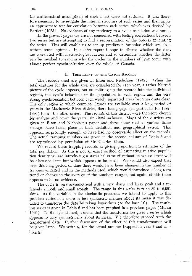
the mathematical assumptions of such a test were not satisfied. It was therefore necessary to investigate the internal structure of each series and then apply an approximate test for correlation between such series, which was devised by Bartlett (1935). No evidence of any tendency to a cyclic oscillation was found.

In the present paper we are not concerned with testing correlations between two series but are attempting to find a representation of the process generating the series. This will enable us to set up prediction formulae which are, in a certain sense, optimal. In a later report I hope to discuss whether the data are correlated with meteorological factors and so determine whether the latter can be invoked to explain why the cycles in the numbers of lynx occur with almost perfect synchronization over the whole of Canada.

11. TREATMEXT OF THE CATCH RECORDS

The records used are given in Elton and Nicholson (1942). When the total captures for the whole area are considered for each year, a rather blurred picture of the cycle appears, but on splitting up the records into the individual regions, the cyclic behaviour of the population in each region and the very strong synchronization between even widely separated areas becomes quite clear. The only region in which complete figures are available over a long period of years is the Mackenzie River district, there being gaps ( in particular for 1892- 1896) for all the other series. The records of this district were therefore chosen for analysis and cover the years 1821-1934 inclusive. Maps of the districts are given in Elton and Nicholson's paper and these show that at various times changes have taken place in their definition and geographical extent. This appears, surprisingly enough, to have had no observable effect on the records. The actual trapping numbers are given in the second column of Table 6 and are reproduced by permission of Mr. Charles Elton.

We regard these trapping records as giving proportionate estimates of the total population. As this is not an exact method of estimating relative population density we are introducing a statistical error of estimation whose effect will be discussed later but which appears to be small. We would also expect that over this long period of time there would have been changes in the number of trappers engaged and in the methods used, which would introduce a long-term trend or change in the average of the numbers caught, but again, of this there appears to be no evidence.

The cycle is very asymmetrical with a very sharp and large peak and a re- latively smooth and small trough. The range in this series is from 39 to 6,991 skins. As the variable in the stochastic processes we intend to apply to this problem varies in a more or less symmetric manner about its mean it was de- cided to transform the data by taking logarithms ( to the base 10). The result- ing series is given in Table 6 and has been graphed in a previous paper (Moran 1949). To the eye, at least, it seems that the transformation gives a series which appears to vary symmetrically about its mean. We therefore proceed with the transformed data. Further discussion of the effect of this transformation will be given later. We write yt for the actual number trapped in year t and xt = log,, yt.

STATISTICAL ANALYSIS OF CANADIAN LYNX CYCLE. I 165

The two main problems which now confront the biologist are to explain why this clearly marked oscillation occurs, and to explain why it occurs in synchronization over the whole of Canada. No plausible theory which will answer both these questions has yet been put forward.

One type of theory suggests that the population density is directly and strongly dependent on some meteorological or other terrestrial phenomenon which itself shows definite oscillations and that these oscillations induce those of the population. An example of such a theory is the idea that the lynx cycle was related to the sunspot cycle. Examination of the data shows that this is impossible oran an 1949) since the cycles are sometimes in phase and sometimes completely out of phase. Other meteorological phenomena have been put forward but it does not seem that there is, as yet, any clear evidence of such a governing cycle. However, one advantage of this type of theory is that it would also explain the synchronization.

Alternatively it may be supposed that the oscillations arise from the population dynamics of the lynx themselves. I t is known that the main food of the lynx is the snowshoe rabbit and that such a predator-prey relationship can easily result in an oscillatory process. However, random influences will affect the process and such random effects will show themselves not merely as super- imposed errors in the series of observations but will affect the future course of the cycle and thus become incorporated into the future history of the series. I t follows that meteorological influences, even if not serially correlated and not themselves showing any cyclic behaviour, might well account for the synchronization of the lynx cycle over the whole of Canada provided they themselves act more or less uniformly over the area. I t is hoped to investigate this possibility in a later paper.

Turning now to the mathematical representation of the data, two models suggest themselves. If the explanation of the cycle is of the first type of theory described above, and if in addition the cyclic phenomenon causing the lynx cycle follows a strict mathematical cycle, one suitable model of the observations would be to suppose that

xt-m = a sin (bt -c) + et: . . . . . (1)

where m is the mean of the series, a, b, and c are constant, and ct is a sequence of independent random variables which may be described as 'error.' If the cycle was not of a simple sine wave type further trigonometric terms might be added. The essential feature of this model is that the random element at any given time does not influence the future course of the cycle.

Alternatively, if the lynx cycle is to be explained by the second type of theory above, or if the causal cycle in the first theory is not a strict cycle but some kind of random process, a suitable model will itself have to be some kind of random or stochastic process. Such models of stationary stochastic processes have been extensively studied by statisticians ever since Yule's classical paper (1927) on the analysis of the sunspot cycle. A suitable model is obtained by supposing that the series of values of xi is generated by a relationship of the form

166 P. A. P. MORAN

where m is the mean of the process, al, . . . ah; are constants, and ct is a sequence of independent random variables with zero means and the same standard deviation. In such a case the random element st is itself incorporated into the future course of the process. Such a relationship is known as an autoregressive or linear stochastic difference equation. If such a process can be reasonably regarded as a good representation of the system generating the observed data, and if the oscillations are due to an intrinsic oscillatory tendency in the biological system itself then the synchronization of the cycles over the whole of Canada might well be due to the correlation between the weather at different places, even though there is no intrinsic cycle in the weather itself. This could be in- vestigated by seeing how strongly the residuals calculated from ( 2 ) are correlated with various meteorological phenomena.

To determine statistically what model best fits the observed data we now carry out a correlogram analysis. The series of x's has a mean 2 = 2.9036 and appears to be trend-free. If we split the series into two halves, 1821-1877 and 1878-1934, we get means 2.9111 and 2.8961. Unfortunately no test of significance of the difference of these means is possible because not only are they correlated but they are themselves based on a series of correlated terms. In order, therefore, to calculate the standard error of their difference it would be necessary to know the serial correlations in the series and the estimation of these requires the assumption that the series is trend-free. No doubt an approximate test would be possible but the agreement is so close that this does not seem necessary. The general problem of testing for trend in a series of correlated terms is one which urgently requires the attention of mathematical statisticians. This absence of trend is very remarkable when one remembers that the geographical area covered by the term 'Mackenzie River District' has changed somewhat in the course of time (see the maps given in Elton and Nicholson 1942). Moreover, with the development of Canada between 1821 and 1934 one would expect that the intensity and efficiency of trapping would have changed.

There being no evidence of trend one can proceed to calculate the standard deviation and serial correlations in the ordinary way. The standard deviation was found to be 0.55737. The serial correlation coefficients, r,, of orders s = 1, 2, . . . 27 were found from the formula

wner e

1 " k = - Cx, = 2.9036 and n = 114.

n i=1

The factor n(n - s)-l is introduced because the numerator is based on n - s pairs of values and the denominator on n values. Taking into account the cor-


rections for the means we might well have used ( n - 1 ) ( n - s - 1)-I instead but the difference appears to be negligible. The results of this calculation, which was carried out for me by the computing staff of the Oxford Institute of Statistics, are shown in Table 1.

TABLE 1 VALUES OF r, FOR s = 1,2, . . .27

When r, is plotted against s we obtain a "correlogram," which is here a smooth, oscillating curve which appears to be very slowly decreasing in ampli- tude. We are now in a position to fit to the data a model of the form ( 2 ) . We must first decide on the value of k. To do this we calculate the partial serial correlation coefficients and test their significance in the manner indicated by Quenouille ( 1949). The idea of using partial serial correlation coefficients in this situation is due to Yule (1927). By rls, he denotes the observed correlation between xt and xt-z when the effect of x t - ~ is removed. Similarly he denotes by r14, 23 the observed correlation between xt and xt-3 when the effect of

and xtYz are removed, and so on. It is not difficult to show that

Moreover, it is not difficult to see that this is in fact equal to in the fitting, by least squares, of a regression formula of the type

xt = a l x t - l t . . . . + ~ ~ k - ~ ~ t - k ~ l t et.

Carrying out the calculations we obtain Table 2.

TABLE 2 VALUES OF THE PARTIAL SERIAL CORRELATIOSS

Suffix of r r 5% Level

Quenouille (1949) has sho 1.n that such a partial serial correlation coefficient can be tested for significant deviation from zero in the ordinary manner provided three 'extra' degrees of fretdom are allowed. In the third column of Table 2 we have therefore calculated 1.96 ( n + 3 - p)-t where p = 1, . . . 6. This should be very close to the true 5 per cent. significance level. It will be seen that rl and r13,2 are both highly significant whilst r13, 234 and r16, 2346 would both also be judged significant. I t is curious that Yule (1927) should have found the same partial serial correlations to be large when he calculated them for his series of graduated sunspot numbers (but ntit for the ungraduated series). Table 2 therefore suggests that k should be taken as 2. There is clearly no advantage in taking it as 3 and if we took it as 5 to include the effect of terms which are apparently significant in Table 2 the reduction in the variance of the estimated residuals would be quite small. Changing the notation slightly to agree with conventional practice in dealing with three-termed autoregressive series we therefore fit a relation of the form

xt-m = a(xt-,--m) +b(~,-~-rn). We then fhd

and our estimated generating relationship for the process is

We can estimate the variance of the error term st by the relation (Kendall 1946b, p. 438),

(1 f b ) ((1 -b)2-a2) var ( e t ) = var (x i )

1 -b

If we calculate what the theoretical form of the correlogram should be, assuming the first two serial correlations to have their observed values, we get

STATISTICAL ANALYSIS OF CASADIAN LYSX CYCLE. I 169

a smooth curve which oscillates in the same manner as the empirical correlogram but is much more heavily damped. This wide apparent divergence between the amplitudes of the oscillations in empirical and theoretical correlograms has been repeatedly noticed before in experimental sampling studies (see e.g. Ken- dall 1 9 4 6 ~ ) . No attempt has been made here to carry out the goodness of fit test of the correlogram devised by Quenouille since it was thought that the tests in Table 2 were sufficient.

It is somewhat more difficult to say how far Table 1 enables us to dis- criminate between a model of the type of equation ( 1 ) ( a model of 'concealed periodicities') and a model of the type of equation ( 2 ) . If the model was of the former type, and no further periodic terms were involved, the observed correlogram should approximate to the form

where a and p are constant and I a I < 1. In this case there would be no damping and r, could never be larger than a except for s = 0. I t would seem from Table 1 that there is a genuine, if small, amount of damping and moreover TI

seems definitely larger in absolute value than any of the subsequent peaks or troughs. I t would therefore seem that the autoregressive model is somewhat more plausible. This is just what we would expect if the cyclic behaviour arises from factors endogenous to the biological system.

TABLE 3 ONE-YEAR PREDICTIONS OF x t

Year Predicted x , Error

-0.0,lo -0.144

0.256 0.084 0.044 0.098 0.175 0.124

Formula ( 5 ) can also be used as a prediction formula aad is an optimal one in the least squares sense. To see how it works in practice predictions of xt were made for the years 1927-1934, each prediction being based on the observed values for the two preceding years. These are given in Table 3, to- gether with the actual error of prediction. In Table 6 will be found all the residuals calculated from formula ( 5 ) and these are in fact the errors of prediction. The error in the prediction may be compared with the standard deviation of the distribution of ct, as found above, which is d0.04591 = 0.2143. This error of prediction assumes that the values of m, a, and b are exact, which is not true since they have been estimated-but this should iritroduce only a rela-

170 P. A. P. MORAN

tively small error. I t may also be noticed that the prediction formula (5) has been calculated from data which include the data used in Table 3 as an illus- tration but it is not thought that this is of any consequence.

The results of Table 3, when converted into actual catches of lynx, are given in Table 4.

Year

1927 1928 1929 1930 1931 1932 1933 1934

To predict further ahead than 1 year one simply applies formula (5) repeatedly, first on the two observed values (e.g. those for 1925, 1926), then on the observed value for 1926 and the predicted value for 1927, and so on. Table 5 shows such results for 1927-1934.

TABLE 4 PREDICTED CATCH

Y t I Predicted ye

TABLE 5 PREDICTIOSS OF x,

1537 529 485 662

1000 1590 2657 3396

Year 1 x,

1574 736 269 546 904

1268 1774 2553

Predicted xt Error S.E. Prediction

These predictions would, if prolonged, show oscillations which damp away to the mean value of xt, thus reflecting the uncertainty in the phase for predictions a long way ahead. The standard error of such a prediction can be easily calculated (for details see Stone 1947) and gradually increases to a value equal to the standard deviation of the original series.


111. DISCUSSION

I t will be seen that the above predictions, even for 1 year ahead, are not very good. This is somewhat disappointing, especially when we remember that this is an optimal linear prediction method in the sense of least squares. The results of Table 3 may suggest at first sight that there is some kind of systematic behaviour in the signs of the residuals. (This, if true, would perhaps suggest that the process would be better represented by some kind of non-linear model. ) To check this, the residuals for the whole series were calculated and are given in Table 6. There is no evidence of any systematic behaviour in the signs of the residuals. However, one curious feature deserves notice. There are 112 residuals and the sum of their squares is 5.788; 56 of these residuals correspond to values of xt greater than the mean 2.9036 (actually 2.904 was the value used in the calculation of the residuals) and 56 correspond to values of xt less than 2.9036. However, the sum of squares of the former is equal to 1.781 whilst the sum of squares corresponding to the latter is 4.007. The ratio is 2.250 which would be judged significant at the 1 per cent, level if the two sets could be regarded as random samples from the same normal population, which is not strictly true. Nevertheless this appears to provide strong evidence that our process is not strictly symmetrical, which is not very surprising.

We must also remember that the population of lynx is not exactly propor- tional to the number caught. A better representation would perhaps be obtained by adding to the series generated by (5 ) an additional "error of observation." The fitting of processes defined in this manner is a much more difficult matter. However, we may shortly indicate here what might be the effect on the serial correlations. If there is an observational error of variance u2

in the number caught zjt, then to a first approximation the variance of the error of observation in xt = logloy, will be

This error will contribute to the variance of the series and thus to the denominator of the expression for the serial correlation but it will not contribute to the expectation of the numerator. If we assume that the observational error is that of a Poisson distribution, which is not implausible, we would put U? = yt. We should therefore subtract the average value of

Yt from the estimate of the variance in the denominator of the expression for rt, or what comes to practically the same thing, multiply each yt by

172 P. A. P. MORAN

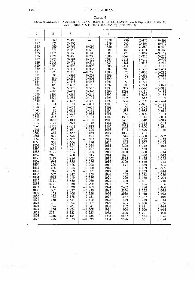
TABLE 6 YEAR (COLUMS I ) , XUIMBER OF LYNX TRAPPED ( x ) (COLUMN 21, )= LOG,, x (COLUMN 3 ) ,

A S D RESIDUALS FROM FORMULA (5) (COLUMN 4)


I have not attempted to calculate E ( ) but the insertion of typical values C

shows that the effect on the estimated serial correlations is small. It is true that the observational error is probably larger than that given by assuming a Poisson distribution but it seems likely that this effect is not large.

Summing up therefore we may say that the series of logarithms of the observed catches is well fitted by an autoregressive scheme and that the data are at least consistent with the idea that the cyclic behaviour is due to factors intrinsic to the biological system. There remains to be explained the synchronization between widely separated areas. To this question I hope to return in a later paper.

1V. REFERENCES BART LET^, M. S. (1935).-Some aspects of the time correlation problem in regard to tests

of significance. J. Roy. Statist. Soc. 98: 536. ELTON, C., and NICHOLSON, M. (1942).-The ten year cycle in numbers of the lynx in

Canada. J. Anim. Ecol. 11: 215-44. KEXDALI., M. G. (1946~)~-"Contributions to the Study of Oscillatory Time Series." (Cam-

bridge Univ. Press. ) KENDALL, M. G. (1949b).-"The Advanced Theory of Statistics." Vol. 2. (Charles Griffin

and Co.: London.) MORAN, P. A. P. (1949).-The statistical analysis of the sunspot and lynx cycles. J . Anim.

Ecol. 18: 115-6. MORAN, P. A. P. (1952).-The statistical analysis of game bird records. J. Anim. Ecol. 21:

154. QUENOUILLE, M. H. (1949).-Approximate tests of correlation in time series. J . Roy. Statist.

SOC. B 11: 68-84. ROWAN, W. ( 1950) .-"Canada's Premier Problem of Animal Conservation." New Biology.

No. 9. (Penguin Books.) STONE, R. (1947).-Prediction from autoregressive schemes. Proc. Internat. Statist. Conf.

1947. Vo1. 5. YULE, G. U. ( 1927) .-On a method of investigating periodicities in disturbed series. Philos.

Trans. 226: 267-98.

The Statistical Analsis of the Canadian Lynx cycle. 1. Structure and Prediction.

Documents

Transcript of The Statistical Analsis of the Canadian Lynx cycle. 1. Structure and Prediction.