arX

iv:a

stro

-ph/

9708

220v

1 2

5 A

ug 1

997

THE STAR FORMATION HISTORY OF FIELD GALAXIES

Piero Madau

Space Telescope Science Institute, 3700 San Martin Drive, Baltimore MD 21218; madau@stsci.edu

Lucia Pozzetti

Dipartimento di Astronomia, Universita di Bologna, via Zamboni 33, I-40126 Bologna;

lucia@astbo3.bo.astro.it

and

Mark Dickinson1,2

Department of Physics and Astronomy, The Johns Hopkins University, Homewood Campus, Baltimore

MD 21218; med@stsci.edu

Received ; accepted

1Also at Space Telescope Science Institute

2Allan C. Davis Fellow

– 2 –

ABSTRACT

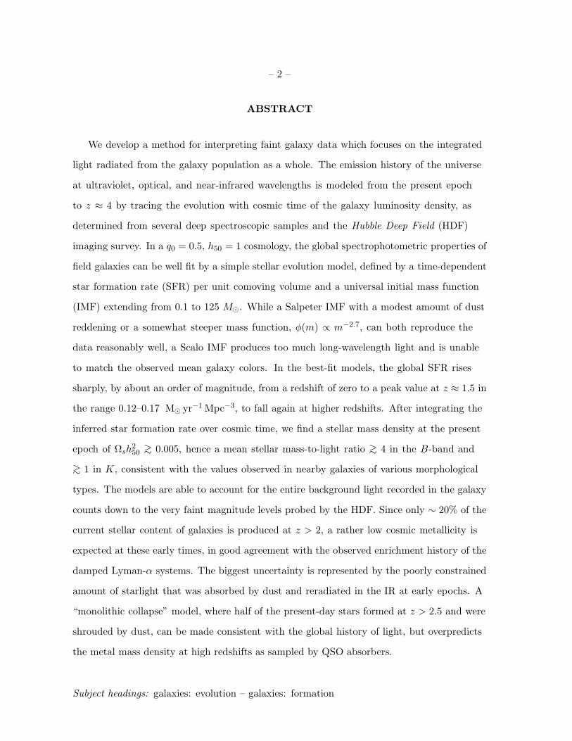
We develop a method for interpreting faint galaxy data which focuses on the integrated

light radiated from the galaxy population as a whole. The emission history of the universe

at ultraviolet, optical, and near-infrared wavelengths is modeled from the present epoch

to z ≈ 4 by tracing the evolution with cosmic time of the galaxy luminosity density, as

determined from several deep spectroscopic samples and the Hubble Deep Field (HDF)

imaging survey. In a q0 = 0.5, h50 = 1 cosmology, the global spectrophotometric properties of

field galaxies can be well fit by a simple stellar evolution model, defined by a time-dependent

star formation rate (SFR) per unit comoving volume and a universal initial mass function

(IMF) extending from 0.1 to 125 M⊙. While a Salpeter IMF with a modest amount of dust

reddening or a somewhat steeper mass function, φ(m) ∝ m−2.7, can both reproduce the

data reasonably well, a Scalo IMF produces too much long-wavelength light and is unable

to match the observed mean galaxy colors. In the best-fit models, the global SFR rises

sharply, by about an order of magnitude, from a redshift of zero to a peak value at z ≈ 1.5 in

the range 0.12–0.17 M⊙ yr−1 Mpc−3, to fall again at higher redshifts. After integrating the

inferred star formation rate over cosmic time, we find a stellar mass density at the present

epoch of Ωsh250 ∼> 0.005, hence a mean stellar mass-to-light ratio ∼> 4 in the B-band and

∼> 1 in K, consistent with the values observed in nearby galaxies of various morphological

types. The models are able to account for the entire background light recorded in the galaxy

counts down to the very faint magnitude levels probed by the HDF. Since only ∼ 20% of the

current stellar content of galaxies is produced at z > 2, a rather low cosmic metallicity is

expected at these early times, in good agreement with the observed enrichment history of the

damped Lyman-α systems. The biggest uncertainty is represented by the poorly constrained

amount of starlight that was absorbed by dust and reradiated in the IR at early epochs. A

“monolithic collapse” model, where half of the present-day stars formed at z > 2.5 and were

shrouded by dust, can be made consistent with the global history of light, but overpredicts

the metal mass density at high redshifts as sampled by QSO absorbers.

Subject headings: galaxies: evolution – galaxies: formation

– 3 –

1. Introduction

In the past few years two different approaches have been widely used to interpret faint galaxy data

(see Ellis 1997 for a recent review). In the simplest version of the “traditional” scheme, a one-to-one

mapping between galaxies at the present epoch and their distant counterparts is assumed: one starts

from the local measurements of the distribution of galaxies as a function of luminosity and Hubble type

and models their photometric evolution assuming some redshift of formation and a set of parameterized

star formation histories (Tinsley 1980; Bruzual & Kron 1980; Koo 1985; Guiderdoni & Rocca-Volmerange

1990; Metcalfe et al. 1991; Gronwall & Koo 1995; Pozzetti, Bruzual, & Zamorani 1996). These, together

with an initial mass function (IMF) and a cosmological model, are then adjusted to match the observed

number counts, colors, and redshift distributions. Beyond the intrinsic simplicity of assuming a well

defined collapse epoch and pure-luminosity evolution thereafter, the main advantage of this kind of

approach is that it can easily be made consistent with the classical view that ellipticals and spiral

galaxy bulges formed early in a single burst of duration 1 Gyr or less (see, e.g. Ortolani et al. 1995

and references therein). Because much of the action happens at high-z, however, these models predict

far more Lyman-break “blue dropouts” than are seen in the Hubble Deep Field (HDF) (Ferguson &

Babul 1997; Pozzetti et al. 1997), and cannot reproduce the rapid evolution – largely driven by late-type

galaxies – of the optical luminosity density with lookback time observed by Lilly et al. (1996) and Ellis

et al. (1996). Less straighforward models which include, e.g., a large population of dwarf galaxies that

begin forming stars at z ≈ 1 (Babul & Ferguson 1996), or do not conserve the number of galaxies due to

merger events (Broadhurst, Ellis, & Glazebrook 1992; Carlberg & Charlot 1993) also appear unable to

match the global properties of present-day galaxies (Ferguson 1997; Ferguson & Babul 1997).

A more physically motivated way to interpret the observations is to construct semianalytic

hierarchical models of galaxy formation and evolution (White & Frenk 1991; Lacey & Silk 1991;

Kauffmann & White 1993; Kauffmann, White, & Guiderdoni 1993; Cole et al. 1994; Baugh et al.

1997). Here, one starts ab initio from a power spectrum of primordial density fluctuations, follows

the formation and merging of dark matter halos, and adopts various prescriptions for gas cooling, star

formation, feedback, and dynamical friction. These are tuned to match the statistical properties of

both nearby and distant galaxies. In this scenario, there is no period when bulges and ellipticals form

rapidly as single units and are very bright: rather, small objects form first and merge continually to

– 4 –

make larger ones. While reasonably successful in recovering the counts, colors, and redshift distributions

of galaxies, a generic difficulty of such models is the inability to simultaneously reproduce the observed

local luminosity density and the zero-point of the Tully-Fisher relation (White & Frenk 1991).

In this paper we shall develop an alternative method, which focuses on the emission properties of

the galaxy population as a whole. It traces the cosmic evolution with redshift of the galaxy luminosity

density – as determined from several deep spectroscopic samples and the HDF imaging survey – and

offers the prospect of an empirical determination of the global star formation history of the universe

and initial mass function of stars independently, e.g., of the merging histories and complex evolutionary

phases of individual galaxies. The technique relies on two basic properties of stellar populations: a) the

UV-continuum emission in all but the oldest galaxies is dominated by short-lived massive stars, and is

therefore a direct measure, for a given IMF and dust content, of the instantaneous star formation rate

(SFR); and b) the rest-frame near-IR light is dominated by near-solar mass evolved stars that make up

the bulk of a galaxy’s stellar mass, and can then be used as a tracer of the total stellar mass density. By

modeling the “emission history” of the universe at ultraviolet, optical, and near-infrared wavelengths

from the present epoch to z ≈ 4, we will shed light on some key questions in galaxy formation and

evolution studies: Is there a characteristic epoch of star and metal formation in galaxies? What fraction

of the luminous baryons observed today were already locked into galaxies at early epochs? Are high-z

galaxies obscured by dust? Do spheroids form early and rapidly? Is there a universal IMF?

Let us point out some of the limitations of our approach at the outset. (1) We shall study the

emission properties of “normal”, optically-selected field galaxies which are only moderately affected by

dust – a typical spiral emits 30% of its energy in the far-infrared region (Saunders et al. 1990). Starlight

which is completely blocked from view even in the near-IR by a large optical depth in dust will not be

recorded by our technique, and the associated baryonic mass and metals missed from our census. The

contribution of infrared-selected dusty starbursts to the present-day total stellar mass density cannot be

very large, however, for otherwise the current limits to the energy density of the mid- and far-infrared

background would be violated (Puget et al. 1996; Kashlinsky, Mather, & Odenwald 1996; Fall, Charlot,

& Pei 1996; Guiderdoni et al. 1997). Locally, infrared luminous galaxies are known to produce only

a small fraction of the IR luminosity of the universe (Soifer & Neugebauer 1991). (2) Our method

bypasses the ambiguities associated with the study of morphologically-distinct samples whose physical

– 5 –

significance remains unclear, but, by the same token, it does not provide any direct information on the

processes which shaped the Hubble sequence. Similarly, this approach does not specifically address the

evolution of particular subclasses of objects, like the oldest ellipticals or low-surface brightness galaxies,

whose star formation history may have differed significantly from the global average (e.g. Renzini 1995;

McGaugh & Bothun 1994). (3) Although in our calculations the IMF extends from 0.1 to 125 M⊙, by

modeling the rest-frame galaxy luminosity density from 0.15 to 2.2 µm we will only be sensitive to stars

within the mass range from ∼ 0.8 to about 20M⊙. This introduces non-negligible uncertainties in our

estimate of the total amount of stars and metals produced. (4) No attempt has been made to include

the effects of cosmic chemical evolution on the predicted galaxy colors. All our population synthesis

models assume solar metallicity, and thus will generate colors that are slightly too red for objects with

low metallicity, e.g. truly primeval galaxies. (5) The uncertanties present in our estimates of the UV

luminosity density from the identification of Lyman-break galaxies in the HDF are quite large, and the

data points at z > 2 should still be regarded as tentative. This is especially true for the faint blue

dropout sample at z ≈ 4, where only one spectroscopic confirmation has been obtained so far (Dickinson

1997). On the other hand, there is no evidence for a gross mismatch at the z ≈ 2 transition between the

photometric redshift sample of Connolly et al. (1997) and the Madau et al. (1996) UV dropout sample.

The initial application of this method was presented by Lilly et al. (1996) and Madau et al. (1996,

hereafter M96). A complementary effort – which starts instead from the analysis of the evolving gas

content and metallicity of the universe – can be found in Fall et al. (1996). Unless otherwise stated, we

shall adopt in the following a flat cosmology with q0 = 0.5 and H0 = 50h50 km s−1 Mpc−1.

2. The Evolution of the Galaxy Luminosity Density

The integrated light radiated per unit volume from the entire galaxy population is an average over

cosmic time of the stochastic, possibly short-lived star formation episodes of individual galaxies, and

will follow a relatively simple dependence on redshift. In the UV – where it is proportional to the global

SFR – its evolution should provide information, e.g., on the mechanisms which may prevent the gas

within virialized dark matter halos from radiatively cooling and turning into stars at early times, or on

the epoch when galaxies exhausted their reservoirs of cold gas. From a comparison between different

wavebands it should be possible to set constraints on the average IMF and dust content of galaxies.

– 6 –

The comoving luminosity density, ρν(z), from the present epoch to z ≈ 4 is given in Table 1 in

five broad passbands centered around 0.15, 0.28, 0.44, 1.0, and 2.2 µm. The data are taken from the

K-selected wide-field redshift survey of Gardner et al. (1997), the I-selected CFRS (Lilly et al. 1996) and

B-selected Autofib (Ellis et al. 1996) surveys, the photometric redshift catalog for the HDF of Connolly

et al. (1997) – which take advantage of deep infrared observations by Dickinson et al. (1997) – and the

color-selected UV and blue “dropouts” of M96. 3 They have all been corrected for incompleteness by

integrating over the best-fit Schechter function in each redshift bin,

ρν(z) =

∫ ∞

0Lνφ(Lν , z)dLν = Γ(2 + α)φ∗L∗. (1)

As it is not possible from the Connolly et al. (1997) and M96 data sets to reliably determine the faint

end slope of the luminosity function, a value of α = −1.3 has been assumed at each redshift interval

for comparison with the CFRS sample (Lilly et al. 1995). The error bars are typically less than 0.2 in

the log, and reflect the systematic uncertainties introduced by the assumption of a particular value of α

and, in the HDF z > 2 sample, in the volume normalization and color-selection region. In the K-band,

the determination by Gardner et al. (1997) agrees to within 30% with Cowie et al. (1996), and we have

assigned an error of 0.1 in the log to the estimate of the local luminosity density at 2.2 µm.

Despite the obvious caveats due to the likely incompleteness in the data sets, different selection

criteria, and existence of systematic uncertainties in the photometric redshift technique, the spectroscopic,

photometric, and Lyman-break galaxy samples appear to provide a remarkably consistent picture of

the emission history of field galaxies. The UV luminosity density rises sharply, by about an order of

magnitude, from a redshift of zero to a peak at z ≈ 1.5, to fall again at higher redshifts (M96; Lilly et

al. 1996; Connolly et al. 1997). This points to a rapid drop in the volume-averaged SFR in the last 8–10

Gyr, and to a redshift range 1 ∼< z ∼< 2 in which the bulk of the stellar population was assembled. The

decline in brightness at late epochs is shallower at longer wavelengths, as galaxies becomes redder with

cosmic time, on the average.

3For the UV dropouts, refined photometric criteria have been used after the many redshift

measurements with the Keck telescope (see Madau 1997a and references therein).

– 7 –

3. Indicators of Past and Present Star Formation Activity

Stellar population synthesis has become a standard technique to study the spectrophotometric

properties of galaxies. Here, we shall make extensive use of the latest version of Bruzual & Charlot (1993)

isochrone synthesis code, optimized with an updated library of stellar spectra (Bruzual & Charlot 1997),

to predict the time change of the spectral energy distribution of a stellar population. The uncertanties

linked to the underlying stellar evolution prescriptions and the lack of accurate flux libraries do not

typically exceed 35% (Charlot, Worthey, & Bressan 1966). Shortward of the Lyman edge, however, the

differences in the predicted ionizing radiation from model atmospheres of hot stars can be quite large

(Charlot 1996a). We shall consider three possibilities for the IMF, φ(m) ∝ m−1−x: a Salpeter (1955)

function (x = 1.35), a Scalo (1986) function, which is flatter for low-mass stars and significantly less rich

in massive stars than Salpeter, and an intermediate case with x = 1.7. In all models the metallicity is

fixed to solar values and the IMF is truncated at 0.1 and 125 M⊙.

3.1. Birthrate–Ultraviolet Relation

The UV continuum emission from a galaxy with significant ongoing star formation is entirely

dominated by late-O/early-B stars on the main sequence. As these have masses ∼> 10M⊙ and lifetimes

tMS ∼< 2×107 yr, the measured luminosity becomes proportional to the stellar birthrate and independent

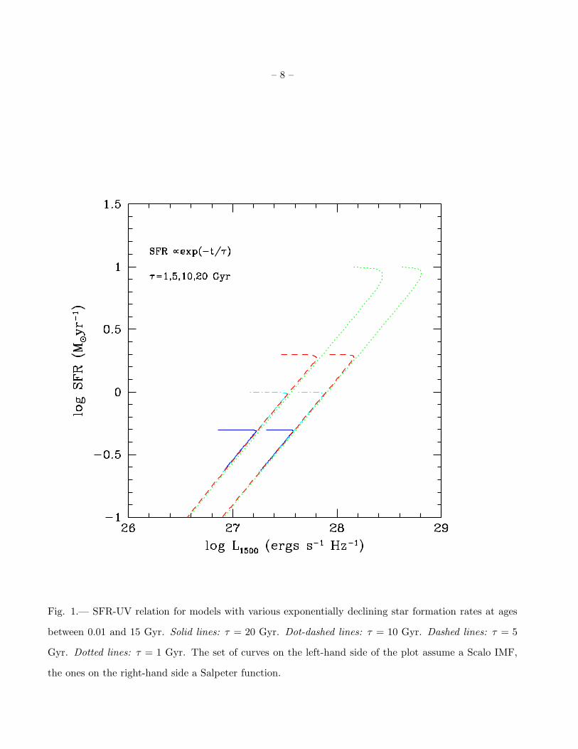
of the galaxy history for t ≫ tMS . This is depicted in Figure 1, where the power radiated at 1500 A

and 2800 A is plotted against the instantaneous SFR for a model stellar population with different star

formation laws, SFR∝ exp(−t/τ), where τ is the duration of the burst. After an initial transient phase

where the UV flux rises rapidly and the turnoff mass drops below 10M⊙, a steady state is reached where

one can write

LUV = const ×SFR

M⊙ yr−1ergs s−1 Hz−1, (2)

with const= (8.0×1027 , 7.9×1027) at (1500A, 2800A) for a Salpeter IMF, and const= (3.5×1027 , 5.1×1027)

for a Scalo IMF, quite insensitive to the details of the past star formation history.4 Note how, for burst

4The luminosities at 1500 A and 2800 A have been averaged over a rectangular bandpass of width

∆λ/λ = 20% in order to approximate the standard broadband filters used in the observations.

– 8 –

Fig. 1.— SFR-UV relation for models with various exponentially declining star formation rates at ages

between 0.01 and 15 Gyr. Solid lines: τ = 20 Gyr. Dot-dashed lines: τ = 10 Gyr. Dashed lines: τ = 5

Gyr. Dotted lines: τ = 1 Gyr. The set of curves on the left-hand side of the plot assume a Scalo IMF,

the ones on the right-hand side a Salpeter function.

– 9 –

durations ∼< 1Gyr and a Scalo IMF, the luminosity at 2800 A becomes a poor SFR indicator after a few

e-folding times, when the contribution of intermediate-mass stars becomes significant. After averaging

over the whole galaxy population, however, we will find that the UV continuum is always a good tracer

of the instantaneous rate of conversion of cold gas into stars.

3.2. Mass–Infrared Relation

If we assume a time-independent IMF, we can then use the results of stellar population synthesis

modeling, together with the observed UV emissivity, to infer the evolution of the star formation activity

in the universe (M96). As already mentioned, the biggest uncertainty in this procedure is due to dust

reddening, as newly formed stars which are completely hidden by dust would not contribute to the UV

luminosity. The effect is potentially more serious at high-z, as for a fixed observer-frame bandpass,

one is looking further into the ultraviolet with increasing redshifts. On the other hand, it should be

possible to test the hypothesis that star formation regions remain, on average, largely unobscured by

dust throughout much of galaxy evolution by looking at the near-infrared light density. This will be

affected by dust only in the most extreme, rare cases, as it takes an E(B − V ) ∼> 4 mag to produce an

optical depth of order unity at 2.2 µm.

Although different types of stars – such as supergiants, AGB, and red giants – dominate the

K-band emission at different ages in an evolving stellar population, the mass-to-infrared light ratio is

relatively insensitive to the star formation history (Charlot 1996b). Figure 2 shows M/LK (in solar

units) as a function of age for models with various exponentially declining SFR compared to the values

observed in nearby galaxies of early to late morphological types.5 As the stellar population ages, the

mass-to-infrared light ratio remains very close to unity, independent of the galaxy color and Hubble type.

We can use this interesting property to estimate the baryonic mass in galaxies from the local K−band

luminosity density, log ρK(0) = 27.05 ± 0.1 h50 ergs s−1 Hz−1 Mpc−3 (Gardner et al. 1997). The observed

range 0.6h50 ∼< M/LK ∼< 1.9h50 translates into a visible (stars+gas) mass density at the present day of

2 × 108∼< ρs+g(0) ∼< 6 × 108 h2

50 M⊙ Mpc−3 (3)

5The observations refer to the mass within the galaxy Holmberg radius, where the contribution by the

dark matter halo is expected to be small (Caldwell & Ostriker 1981).

– 10 –

(0.003 ∼< Ωs+g ∼< 0.009). We shall see in the next section how the observed integrated UV emission, with

or without the addition of some modest amount of reddening, may account for the bulk of the baryons

traced by the K-band light, and how initial mass functions with relatively few high-mass stars (such as

the Scalo IMF), or models with a large amount of dust extinction at all epochs will tend to overproduce

the near-infrared emissivity.

4. Stellar Population Synthesis Modeling

An interesting question now arises as to whether a simple stellar evolution model, defined by a

time-dependent SFR per unit volume and a constant IMF, may reproduce the global UV, optical, and

near-IR photometric properties of the universe as given in Table 1. In a stellar system with arbitrary

star formation rate, the luminosity density at time t is given by the convolution integral

ρν(t) =

∫ t

0Lν(τ) × SFR(t − τ)dτ, (4)

where Lν(τ) is the specific luminosity radiated per unit initial mass by a generation of stars with age τ .

In the instantaneous recycling approximation (Tinsley 1980), the total stellar mass density produced at

time t is

ρs(t) = (1 − R)

∫ t

0SFR(t)dt, (5)

where R is the mass fraction of a generation of stars that is returned to the interstellar medium,

R ≈ 0.3, 0.15, and 0.2 for a Salpeter, x = 1.7, and Scalo IMF, respectively. 6 In computing the time

evolution of the spectrophotometric properties of a stellar population in comoving volumes large enough

to be representative of the universe as a whole, our first task is to relate the observed UV emission to a

SFR density. We assume a universal IMF and fit a smooth function to the UV continuum emissivity at

various redshifts. By construction, all models will then produce, to within the errors, the right amount

of ultraviolet light. We then use Bruzual-Charlot’s synthesis code to predict the cosmic emission history

at long wavelengths.

6To compute the return fraction R we have adopted the semiempirical initial-final mass relation of

Weidemann (1987) for stars with initial masses between 1 and 8 M⊙. Stars with M > 10M⊙ have been

assumed to return all but a 1.4M⊙ remnant.

– 11 –

Fig. 2.— Total (processed gas+stars) mass-to-K band light ratio versus age for models with various

exponentially declining star formation rates. Solid lines: Salpeter IMF. Dotted lines: Scalo IMF. From

top to bottom, each set of curves depict the values for τ = 1, 5, 10, and 20 Gyr, respectively. The data

points show the visible mass-to-infrared light ratio versus B − V color (top axis) observed in nearby

galaxies of various morphological types (Charlot 1996b).

– 12 –

In one of the scenarios discussed in the next section, the effect of dust attenuation will be taken into

account by multiplying equation (4) by pesc, a time-independent term equal to the fraction of emitted

photons which are not absorbed by dust. For purposes of illustration, we assume a foreground screen

model, pesc = exp(−τν), and SMC-type dust. 7 This should only be regarded as an approximation, since

hot stars can be heavily embedded in dust within star-forming regions, there will be variety of extinction

laws, and the dust content of galaxies will evolve with redshift. While the existing data are too sparse

to warrant a more elaborate analysis, this simple approximation well highlights the main features and

assumptions of the model. It is possible to gauge the luminosity-weighted amount of dust extinction at

the present epoch by looking at the observed local far-infrared luminosity density. For normal galaxies,

the emissivity from 8 to 115 µm is estimated from the IRAS survey to be around 30% of their integrated

emission in the B-band (Saunders et al. 1990). Assuming that a negligible fraction of the ionizing flux

emerges in nebular lines, and a Salpeter IMF, this value implies a small luminosity-weighted color excess,

E(B − V ) ≈ 0.012 (τB ≈ 0.025). The Calzetti, Kinney, & Storchi-Bergmann (1994) empirical extinction

law for starbursts, normalized to A(V )/E(B − V ) = 4.88, yields a mean dust opacity that is similarly

low.

4.1. Salpeter IMF

Figure 3 shows the model predictions for the evolution of ρν at rest-frame ultraviolet to near-infrared

frequencies. The data points with error bars are taken from Table 1, and a Salpeter IMF has been

assumed. In the absence of dust reddening, this relatively flat IMF generates spectra that are too blue

to reproduce the observed mean (luminosity-weighted over the entire population) galaxy colors. The

shape of the predicted and observed ρν(z) relations agrees better to within the uncertainties if some

amount of dust extinction, E(B − V ) = 0.1, is included. In this case, the observed UV luminosities must

be corrected upwards by a factor of 1.4 at 2800 A and 2.1 at 1500 A. As expected, while the ultraviolet

emissivity traces remarkably well the rise, peak, and sharp drop in the instantaneous star formation

7Since what is relevant here is the absorption opacity, we have multiplied the extinction optical depth

by a factor of 0.6, as the albedo of dust grains is known to approach asymptotically 0.4–0.5 at ultraviolet

wavelengths (e.g., Pei 1992).

– 13 –

Fig. 3.— Evolution of the luminosity density at rest-frame wavelengths of 0.15 (dotted line), 0.28 (solid

line), 0.44 (short-dashed line), 1.0 (long-dashed line), and 2.2 (dot-dashed line) µm. The data points with

error bars are taken from Lilly et al. (1996) (filled dots at 0.28, 0.44, and 1.0 µm), Connolly et al. (1997)

(empty squares at 0.28 and 0.44 µm), Madau et al. (1996) and Madau (1997a) (filled squares at 0.15 µm),

Ellis et al. (1996) (empty triangles at 0.44 µm), and Gardner et al. (1997) (empty dot at 2.2 µm). The

inset in the upper-right corner of the plot shows the SFR density (M⊙ yr−1 Mpc−3) versus redshift which

was used as input to the population synthesis code. The model assumes a Salpeter IMF, SMC-type dust

in a foreground screen, and a universal E(B − V ) = 0.1.

– 14 –

rate (the smooth function shown in the inset on the upper-right corner of the figure), an increasingly

large component of the longer wavelengths light reflects the past star formation history. The peak in

the luminosity density at 1.0 and 2.2 µm occurs then at later epochs, while the decline from z ≈ 1 to

z = 0 is more gentle than observed at shorter wavelengths. The total stellar mass density at z = 0 is

ρs(0) = 3.7 × 108 M⊙ Mpc−3, with a fraction close to 65% being produced at z > 1, and only 20% at

z > 2. In the assumed cosmology, about half of the stars observed today are more than 9 Gyr old, and

only 20% are younger than 5 Gyr.8

4.2. x=1.7 IMF

Figure 4 shows the model predictions for a x = 1.7 IMF and negligible dust extinction. While

able to reproduce quite well the B-band emission history and consistent within the error with the local

K-band light, this model slightly underestimates the 1 µm luminosity density at z ≈ 1. The total stellar

mass density today is larger than in the previous case, ρs(0) = 6.2 × 108 M⊙ Mpc−3.

4.3. Scalo IMF

Figure 5 shows the model predictions for a Scalo IMF. The fit to the data is now much poorer, since

this IMF generates spectra that are too red to reproduce the observed mean galaxy colors, as first noted

by Lilly et al. (1996). Because of the relatively large number of solar mass stars formed, it produces too

much long-wavelength light by the present epoch. The addition of dust reddening would obviously make

the fit even worse. The total stellar mass density produced is similar to the Salpeter IMF case.

5. Clues to Galaxy Formation and Evolution

The results shown in the previous section have significant implications for our understanding of

the global history of star and structure formation. Here we discuss a few key issues which will assist in

8Note that, unlike the measured number densities of objects and rates of star formation, the integrated

stellar mass density does not depend on the assumed cosmological model.

– 15 –

Fig. 4.— Same as in Figure 3, but assuming an IMF with φ(m) ∝ m−1−1.7 and no dust extinction.

– 16 –

Fig. 5.— Same as in Figure 3, but assuming a Scalo IMF and no dust extinction. This model overproduces

the local K-band emissivity by a factor of 2.

– 17 –

interpreting the evolution of luminous matter in the universe.

5.1. Extragalactic Background Light

Our modeling of the data points to the redshift range where the bulk of the stellar mass was

actually produced: 1 ∼< z ∼< 2. The uncertainties in the determination of the luminosity density at that

epoch are, however, quite large. At z ≈ 1, the increase in the “estimated” emissivity (i.e., corrected for

incompleteness by integrating over the best-fit Schechter function) over that “directly” observed in the

CFRS galaxy sample is about a factor of 2 (Lilly et al. 1996). Between z = 1 and z = 2, the peak in the

average SFR is only constrained by the photometric redshifts of Connolly et al. (1997) and by the HDF

UV dropout sample, both of which may be subject to systematic biases.

An important check on the inferred emission history of field galaxies comes from a study of the

extragalactic background light (EBL), an indicator of the total optical luminosity of the universe. The

contribution of known galaxies to the EBL can be calculated directly by integrating the emitted flux

times the differential galaxy number counts down to the detection threshold. We have used a compilation

of ground-based and HDF data down to very faint magnitudes (Pozzetti et al. 1997; Williams et al.

1996) to compute the mean surface brightness of the night sky between 0.35 and 2.2 µm. The results are

plotted in Figure 6, along with the EBL spectrum predicted by our modeling of the galaxy luminosity

density,

Jν =1

4π

∫ ∞

0dz

dl

dzρν′(z) (6)

where ν ′ = ν(1 + z) and dl/dz is the cosmological line element. The overall agreement is remarkably

good, with the model spectra being only slightly bluer, by about 20–30%, than the observed EBL. The

straightforward conclusion of this exercise is that the star formation histories depicted in Figures 3 and

4 appear able to account for the entire background light recorded in the galaxy counts down to the very

faint magnitudes probed by the HDF.

– 18 –

Fig. 6.— Spectrum of the extragalactic background light as derived from a compilation of ground-based

and HDF galaxy counts (see Pozzetti et al. 1997). The 2σ error bars arise mostly from field-to-field

variations. Solid line: Model predictions for a Salpeter IMF and E(B − V ) = 0.1 (star formation history

of Figure 3). Dotted line: Model predictions for a x = 1.7 IMF and negligible dust extinction (star

formation history of Figure 4).

– 19 –

5.2. The Stellar Mass Density Today

The best-fit models discussed in § 4 generate a present-day stellar mass density in the range between

4 and 6 ×108 M⊙ Mpc−3 (0.005 ∼< Ωsh250 ∼< 0.009). Although one could in principle reduce the inferred

star formation density by adopting a top-heavy IMF, richer in massive UV-producing stars, in practice

a significant amount of dust reddening – hence of “hidden” star formation – would then be required to

match the observed galaxy colors. The net effect of this operation would be a large infrared background

(see below). The stellar mass-to-light ratios range from 4.5 in the B-band and 0.9 in K for a Salpeter

function, to 8.1 in B and 1.5 in K for a x = 1.7 IMF. Note that these values are quite sensitive to the

lower-mass cutoff of the IMF, as very-low mass stars can contribute significantly to the mass but not

to the integrated light of the whole stellar population. A lower cutoff of 0.2M⊙ instead of the 0.1M⊙

adopted would decrease the mass-to-light ratio by a factor of 1.3 for a Salpeter function, 1.6 for x = 1.7,

and 1.1 for a Scalo IMF.

5.3. The Star Formation Density Today

The predicted local rate of star formation ranges between 0.95×10−2 (Salpeter) and

1.6×10−2 M⊙ yr−1 Mpc−3 (x = 1.7). According to Gallego et al. (1995), the Hα luminosity

density of the local universe is log ρHα = 39.1± 0.04 ergs s−1 Mpc−3. Let us assume case-B recombination

theory, and adopt the mean unreddened spectrum at z = 0 corresponding to the Salpeter IMF model,

i.e., assume the emitted ionizing photons are converted to Hα radiation before being absorbed by dust.

The Hα luminosity density can then be related to the local SFR per unit volume according to

log ρHα = 39.2 + log

(

SFR

0.01M⊙ yr−1 Mpc−3

)

ergs s−1 Mpc−3, (7)

(the coefficient for the x = 1.7 case is 38.6) and is in good agreement with the Gallego et al.

determination. Very recently, we became aware of the first results of an ongoing redshift survey of

galaxies imaged in the rest-frame ultraviolet at 2000 A with the FOCA balloon-borne camera (Treyer et

al. 1997; Milliard et al. 1992). The light density resulting from the integrated emission of the observed

galaxies, which have mean redshift 〈z〉 = 0.15, is ρ2000 = 8.0± 0.35× 1025 h50 ergs s−1 Hz−1 Mpc−3, again

in reasonable agreement with the predicted value of ≈ 5 × 1025 h50 ergs s−1 Hz−1 Mpc−3.

– 20 –

5.4. Star Formation at High Redshift: Monolithic Collapse Versus Hierarchical

Clustering Models

We have already cautioned the reader against the significant uncertanties present in our estimates

of the star formation density at z > 2. The biggest one is probably associated with dust reddening,

but, as the color-selected HDF sample includes only the most actively star-forming young objects, one

could also imagine the existence of a large population of relatively old or faint galaxies still undetected

at high-z. The issue of the amount of star formation at early epochs is a non trivial one, as the two

competing models, “monolithic collapse” versus hierarchical clustering, make very different predictions

in this regard. From stellar population studies we know in fact that about half of the present-day

stars are contained in spheroidal systems, i.e., elliptical galaxies and spiral galaxy bulges (Schechter &

Dressler 1987). In the monolithic scenario these formed early and rapidly, experiencing a bright starburst

phase at high-z (Eggen, Lynden-Bell, & Sandage 1962; Tinsley & Gunn 1976; Bower et al. 1992). In

hierarchical clustering theory, instead, objects form and grow throughout the history of the universe by

a process of mergers and accretion (White & Frenk 1991; Searle & Zinn 1978). In such models, elliptical

galaxies form late by mergers of roughly equal mass disks (Kauffmann et al. 1993), and most galaxies

never experience star formation rates in excess of a few solar masses per year (Baugh et al. 1997). The

star formation histories discussed in § 4 produce only 20% of the current stellar content of galaxies at

z > 2, in apparent agreement with hierarchical clustering theories. In fact, the tendency to form the

bulk of the stars at relatively low redshifts is a generic feature not only of the Ω0 = 1 CDM cosmology,

but also of successful low-density CDM models (cf Figure 21 of Cole et al. 1994; Baugh et al. 1997).

It is then of interest to ask how much larger could the volume-averaged SFR at high-z be before its

fossil records – in the form of long-lived, near solar-mass stars – became easily detectable as an excess

of K-band light at late epochs. In particular, is it possible to envisage a toy model where 50% of the

present-day stars formed at z > 2.5 and were shrouded by dust? The predicted emission history from

such a scenario is depicted in Figure 7. To minimize the long-wavelength emissivity associated with the

radiated ultraviolet light, a Salpeter IMF has been adopted. Consistency with the HDF data has been

obtained assuming a dust extinction which increases rapidly with redshift, E(B − V ) = 0.011(1 + z)2.2.

This results in a correction to the rate of star formation of a factor ∼ 5 at z = 3 and ∼ 15 at z = 4. The

total stellar mass density today is ρs(0) = 5.0 × 108 M⊙ Mpc−3 (Ωsh250 =0.007).

– 21 –

Overall, the fit to the data is still acceptable, showing how the blue and near-IR light at z < 1 are

relatively poor indicators of the star formation history at early epochs. The reason for this is the short

timescale available at z ∼> 2, which makes the present-day stellar mass density rather insensitive to a

significant boost of the stellar birthrate at high redshifts. By contrast, variations in the global SFR

around z ∼ 1.5, where the bulk of the stellar population was assembled, have a much larger impact.

The adopted extinction-redshift relation, in fact, implies negligible reddening at z ∼< 1. Relaxing this

– likely unphysical – assumption would cause the model to significantly overproduce the K-band local

luminosity density. We have also checked that a larger amount of hidden star formation at early epochs,

as recently advocated by Meurer et al. (1997), would generate too much blue, 1 µm and 2.2 µm light

to be still consistent with the observations. An IMF which is less rich in massive stars would only

exacerbate the discrepancy.

5.5. The Colors of High-Redshift Galaxies

Figure 8 shows a comparison between the HDF data and the model predictions for the evolution of

galaxies in the U − B vs. V − I color-color plane according to the star formation histories of Figures

3 and 4. The HDF ultraviolet passband – which is bluer than the standard ground-based U filter –

permits the identification of star-forming galaxies in the interval 2 ∼< z ∼< 3.5. Galaxies in this redshift

range predominantly occupy the top left portion of the U − B vs. V − I color-color diagram because of

the attenuation by the intergalactic medium and intrinsic absorption (M96). Galaxies at lower redshift

can have similar U − B colors, but are typically either old or dusty, and are therefore red in V − I as

well. The fact that the Salpeter IMF, E(B − V ) = 0.1 model reproduces quite well the rest-frame UV

colors of high-z galaxies, while a dust-free x = 1.7 IMF generates V − I colors that are 0.2 mag too blue,

suggests the presence of some amount of dust extinction in Lyman-break galaxies at z ∼ 3 (Meurer et

al. 1997; Dickinson et al. 1997). Adopting the greyer extinction law deduced by Calzetti et al. (1994)

from the integrated spectra of nearby starbursts would require larger corrections to the SFR at high-z

in order to match the observed colors. The consequence of this, however, would be the overproduction

of red light at low redshifts, as noted in § 5.4. Redder spectra can also result from an aging population

or an IMF which is less rich in massive stars than the adopted ones.

– 22 –

Fig. 7.— Test case with a much larger star formation density at high redshift than indicated by the HDF

dropout analysis. The model – designed to mimick a “monolithic collapse” scenario – assumes a Salpeter

IMF and a dust opacity which increases rapidly with redshift, E(B − V ) = 0.011(1 + z)2.2. Notation is

the same as in Figure 3.

– 23 –

Fig. 8.— Solid lines: model predictions for the color evolution of galaxies according to the star formation

histories of Figure 3 (right curve) and 4 (left curve). The points (filled squares for z > 2 and empty squares

for z < 2) are plotted at redshift interval ∆z = 0.1. Empty circles and triangles: colors of galaxies in

the HDF with 22 < B < 27. Objects undetected in U (with S/N < 1) are plotted as triangles at the 1σ

lower limits to their U − B colors. Symbols size scales with the I mag of the object, and all magnitudes

are given in the AB system. The “plume” of reddened high-z galaxies is clearly seen in the data.

– 24 –

5.6. Constraints from the Mid- and Far-Infrared Background

Ultimately, it should be possible to set some constraints on the total amount of star formation that

is hidden by dust over the entire history of the universe by looking at the cosmic infrared background

(CIB) (Fall et al. 1996; Burigana et al. 1997; Guiderdoni et al. 1997). Studies of the CIB provide

information which is complementary to that given by optical observations. If most of the star formation

activity takes place within dusty gas clouds, the starlight which is absorbed by various dust components

will be reradiated thermally at longer wavelengths according to characteristic IR spectra. The energy

in the CIB would then exceed by far the entire background optical light which is recorded in the galaxy

counts.

From an analysis of the smoothness of the COBE DIRBE maps, Kashlinsky et al. (1996) have

recently set an upper limit to the CIB of 10–15 nW m−2 sr−1 at λ =10–100 µm assuming clustered

sources which evolve according to typical scenarios. An analysis using data from COBE FIRAS by Puget

et al. (1996) (see also Fixsen et al. 1996) has revealed an isotropic residual at a level of 3.4 (λ/400µm)−3

nW m−2 sr−1 in the 400–1000 µm range, which could be the long-searched CIB. The detection, recently

revisited by Guiderdoni et al. (1997), should be regarded as uncertain since it depends critically on the

subtraction of foreground emission by interstellar dust.

By comparison, the total amount of starlight that is absorbed by dust and reprocessed in the

infrared is 7.5 nW m−2 sr−1 in the model depicted in Figure 3, about 30% of the total radiated flux. The

monolithic collapse scenario of Figure 7 generates 6.5 nW m−2 sr−1 instead. The resulting CIB spectrum

is expected to be rather flat because of the spread in the dust temperatures – cool dust will likely

dominate the long wavelength emission, warm small grains will radiate mostly at shorter wavelengths –

and the distribution in redshift. While both models appear then to be consistent with the data (given

the large uncertainties associated with the removal of foreground emission and with the observed and

predicted spectral shape of the CIB), it is clear that too much infrared light would be generated by

scenarios that have significantly larger amount of hidden star formation at early and late epochs.

– 25 –

5.7. Metal Production

We may at this stage use our set of models to establish a cosmic timetable for the production of

heavy elements (with atomic number Z ≥ 6) in relatively bright field galaxies (see M96). What we are

interested in here is the universal rate of ejection of newly synthesized material. In the approximation

of instantaneous recycling, the metal ejection rate per unit comoving volume can be written as

ρZ = y(1 − R) × SFR, (8)

where the net, IMF-averaged yield of returned metals is

y =

∫

mpzmφ(m)dm

(1 − R)∫

mφ(m)dm, (9)

pzm is the stellar yield, i.e., the mass fraction of a star of mass m that is converted to metals and ejected,

and the dot denotes differentiation with respect to cosmic time.

The predicted end-products of stellar evolution, particularly from massive stars, are subject to

significant uncertainties. These are mainly due to the effects of initial chemical composition, mass-loss

history, the mechanisms of supernova explosions, and the critical mass, MBH, above which stars collapse

to black holes without ejecting heavy elements into space. To be quantitative, let us compare the

nucleosynthetic enrichment from massive stars (m ≥ 9M⊙) according to the chemical yields tabulated

by various authors. For a Salpeter IMF, the total amount of freshly produced metals expelled in winds

and final ejecta (in supernovae or planetary nebulae) gives, according to Maeder (1992), y = 0.022 for

initial solar metallicity, high mass-loss rates, and MBH = 120M⊙. When mass loss is small, as it is

believed to be the case for low metallicities, the net yield increases to y = 0.027. The Type II stellar

yields without mass loss tabulated by Woosley & Weaver (1995) give y = 0.014 (with MBH = 40M⊙

and Z = Z⊙), those of Tsujimoto et al. (1995) y = 0.024 (with MBH = 70M⊙ and Z = Z⊙). These

values are very sensitive to the choice of the IMF slope and lower-mass cutoff. For a Scalo IMF in the

assumed mass range (0.1 < M < 125M⊙), the net yield is typically a factor of 3.3 lower than Salpeter,

and a factor of 4.5 lower for x = 1.7. At the same time, a lower cutoff of 0.5M⊙ would boost the

net yield by a factor of 1.9 for Salpeter, 1.7 for Scalo, and 3.1 for x = 1.7. Note that some of these

ambiguities partially cancel out when computing the total metal ejection rate, as the product y × SFR

is less sensitive to the slope of the IMF than the yield or the rate of star formation, and is insensitive

to the lower mass cutoff. Observationally, the best-fit “effective yield” (derived assuming a closed box

– 26 –

model) is 0.025Z⊙ for Galactic halo clusters, 0.3Z⊙ for disk clusters, 0.4Z⊙ for the solar neighborhood,

and 1.8Z⊙ for the Galactic bulge (Pagel 1987). The last value may represent the universal true yield,

while the lower effective yields found in the other cases may be due, e.g., to the loss of enriched material

in galactic winds.

Figure 9 shows the total mass of metals ever ejected, ρZ , versus redshift, i.e., the sum of the heavy

elements stored in stars and in the gas phase as given by the integral of equation (8) over cosmic time.

The values plotted have been computed from the star formation histories depicted in Figures 3 and 7,

and have been normalized to yρs(0), the mass density of metals at the present epoch according to each

model. A characteristic feature of the two competing scenarios is the rather different average metallicity

expected at high redshift. For comparison, we have also plotted the gas metallicity, ZDLA/Z⊙, as

deduced from observations by Pettini et al. (1997) of the damped Lyman-α systems (DLAs). At early

epochs, when the gas consumption into stars is still low, the metal mass density predicted from these

models gives, in a closed box model, a measurement of the metallicity of the gas phase. If DLAs and

star-forming field galaxies have the same level of heavy element enrichment, then one would expect

a rough agreement between ZDLA and the model predictions at z ∼> 3. This is not true at z ∼< 2,

when a significant fraction of heavy elements is locked into stars.9 Without reading too much into

this comparison, it does appear that the monolithic collapse scenario tends to overpredict the cosmic

metallicity at high redshifts as sampled by the DLAs. In order for such a model to be acceptable, the gas

traced by DLAs would have to be physically distinct from the luminous star formation regions observed

in the Lyman-break galaxies, and to be substantially under-enriched in metals compared to the cosmic

mean.

It has been recently pointed out by Renzini (1997) and Mushotzky & Loewenstein (1997) that, in

the absence of any systematic cluster/field differences, clusters of galaxies may also provide an indication

of the metal formation history of the universe. In the Salpeter IMF model of Figure 3, the global

metallicity of the local universe is yΩs/Ωb ≈ 0.1y/Z⊙ solar, to be compared with the overall cluster metal

abundance, ∼ 1/3 solar. If y ∼ Z⊙, the efficiency of metal production must have been larger in clusters

9More complex chemical evolution models which reproduce the metal enrichement history of the DLAs

can be found in Pei & Fall (1995).

– 27 –

than in the field, in spite of both having a similar baryon-to-star conversion efficiency, Ωs/Ωb ∼ 10%

(Renzini 1997). Alternatively, a yield y ∼ 3Z⊙ may solve the apparent discrepancy. In this case, field

galaxies would have to have ejected a significant amount of the heavy elements they produced, and there

should be a comparable share of metals in the intergalactic medium (IGM) as there is in the intracluster

gas.

We have benefited from many stimulating discussions with G. Bruzual, D. Calzetti, S. Charlot, M.

Fall, N. Panagia, M. Pettini, and A. Renzini on various topics related to this work. We are indebted

to G. Bruzual and S. Charlot for providing the newer population synthesis models, to A. Connolly

for computing the B-band luminosity density from his photometric redshift catalog, and to M. Treyer

and R. Ellis for communicating their unpublished results on the local UV luminosity function. We

thank the referee, Raja Guhathakurta, for carefully reading the manuscript and for valuable comments.

Support for this work was provided by NASA through grants NAG5-4236 and AR-06337.10-94A from

the Space Telescope Science Institute, which is operated by the Association of Universities for Research

in Astronomy, Inc., under NASA contract NAS5-26555.

– 28 –

Fig. 9.— Total mass of heavy elements ever ejected versus redshift for the Salpeter IMF model of Figure

3 (dashed line) and the “monolithic collapse” model of Figure 7 (dotted line), normalized to yρs(0), the

total mass density of metals at the present epoch. Filled squares: column density-weighted metallicities

(in units of solar) as derived from observations of the damped Lyman-α systems (Pettini et al. 1997).

– 29 –

Table 1. Comoving Luminosity Densitya

redshift 1500 A 2800 A 4400 A 1 µm 2.2 µm

Gardner et al. (1997)

0.0 · · · · · · · · · · · · 27.05±0.1

Lilly et al. (1996)

0.20–0.50 · · · 25.89±0.07 26.63±0.07 27.26±0.08 · · ·

0.50–0.75 · · · 26.21±0.08 26.86±0.08 27.36±0.07 · · ·

0.75–1.00 · · · 26.53±0.15 27.05±0.13 27.50±0.11 · · ·

Ellis et al. (1996)

0.0 · · · · · · 26.49±0.10 · · · · · ·

0.02–0.15 · · · · · · 26.53±0.08 · · · · · ·

0.15–0.35 · · · · · · 26.58±0.08 · · · · · ·

Connolly et al. (1997)

0.50–1.00 · · · 26.52±0.15 27.03±0.15 · · · · · ·

1.00–1.50 · · · 26.69±0.15 27.12±0.15 · · · · · ·

1.50–2.00 · · · 26.59±0.15 27.03±0.15 · · · · · ·

Madau et al. (1996) and Madau (1997a)

2.00–3.50 26.42±0.15 · · · · · · · · · · · ·

3.50–4.50 26.02±0.20 · · · · · · · · · · · ·

aValues listed are log luminosity density in units of h50 ergs s−1 Hz−1 Mpc−3.

– 30 –

REFERENCES

Babul, A., & Ferguson, H. C. 1996, ApJ, 458, 100

Baugh, C. M., Cole, S., Frenk, C. S., & Lacey, C. G. 1997, ApJ, submitted

Bower, R. G., Lucey, J. R., & Ellis, R. S. 1992, MNRAS, 254, 589

Broadhurst, T. J., Ellis, R. S., & Glazebrook, K. 1992, Nature, 355, 55

Bruzual, A. G., & Charlot, S. 1993, ApJ, 405, 538

Bruzual, A. G., & Charlot, S. 1997, in preparation

Bruzual A. G., & Kron, R. G. 1980, ApJ, 241, 25

Burigana, C., Danese, L., De Zotti, G., Franceschini, A., Mazzei, P., & Toffolatti, L. 1997, MNRAS, 287,

L17

Caldwell, J. A. R., & Ostriker, J. P. 1981, ApJ, 251, 61

Calzetti, D., Kinney, A. L., & Storchi-Bergmann, T. 1994, ApJ, 429, 582

Carlberg, R. G., & Charlot, S. 1992, ApJ, 397, 5

Charlot, S. 1996a, in From Stars to Galaxies, eds. C. Leitherer & U. Fritze-von Alvensleben (ASP

Conference Series), in press

Charlot, S. 1996b, in The Universe at High-z, Large Scale Structure, and the Cosmic Microwave

Background, eds. E. Martinez-Gonzalez & J. L. Sanz (Heidelberg: Springer), p. 53

Charlot, S., Worthey, G., & Bressan, A. 1996, ApJ, 457, 625

Cole, S., Aragon-Salamanca, A., Frenk, C. S., Navarro, J. F., & Zepf, S. E. 1994, MNRAS, 271, 781

Connolly, A. J., Szalay, A. S., Dickinson, M. E., SubbaRao, M. U., & Brunner, R. J. 1997, ApJ, in press

Cowie, L. L., Songaila, A., Hu, E. M., & Cohen, J. G. 1996, AJ, 112, 839

Dickinson, M. E. 1997, private communication

Dickinson, M. E., et al. 1997, in preparation

Eggen, O. J., Lynden-Bell, D., & Sandage, A. R. 1962, ApJ, 136, 748

Ellis, R. S. 1997, ARA&A, 35, in press

– 31 –

Ellis, R. S., Colless, M., Broadhurst, T., Heyl, J., & Glazebrook, K. 1996, MNRAS, 280, 235

Fall, S. M., Charlot, S., & Pei, Y. C. 1996, ApJ, 464, L43

Ferguson, H. C. 1997, in The Hubble Space Telescope and the High Redshift Universe, eds. N. R.

Tanvir, A. Aragon-Salamanca, & J. V. Wall, (Singapore: World Scientific Press), in press

Ferguson, H. C., & Babul, A. 1997, MNRAS, in press

Fixsen, D. J., Cheng, E. S., Gales, J. M., Mather, J. C., Shafer, R. A., Wright, E. L. 1996, ApJ, 473, 576

Gallego, J., Zamorano, J., Aragon-Salamanca, A., & Rego, M. 1995, ApJ, 455, L1

Gardner, J. P., Sharples, R. M., Frenk, C. S., & Carrasco, B. E. 1997, ApJ, 480, L99

Gronwall, C., & Koo, D. C. 1995, ApJ, 440, L1

Guiderdoni, B., Bouchet, F. R., Puget, J.-L., Lagache, G., & Hivon, E. 1997, Nature, in press

Guiderdoni, B., & Rocca-Volmerange, B. 1990, A&A, 227, 362

Kashlinsky, A., Mather, J. C., & Odenwald, S. 1996, ApJ, 473, L9

Kauffmann, G., & White, S. D. M. 1993, MNRAS, 261, 921

Kauffmann, G., White, S. D. M., & Guiderdoni, B. 1993, MNRAS, 264, 201

Koo, D. C. 1985, AJ, 90, 418

Lacey, C. G., & Silk, J. 1991, ApJ, 381, 14

Lilly, S. J., Le Fevre, O., Hammer, F., & Crampton, D., 1996, ApJ, 460, L1

Lilly, S. J., Tresse, L., Hammer, F., Crampton, D., & Le Fevre, O. 1995, ApJ, 455, 108

Madau, P. 1997a, in Star Formation Near and Far, eds. S. S. Holt & G. L. Mundy, (AIP: New York), p.

481

Madau, P., Ferguson, H. C., Dickinson, M. E., Giavalisco, M., Steidel, C. C., & Fruchter, A. 1996,

MNRAS, 283, 1388 (M96)

Maeder, A. 1992, A&A, 264, 105

McGaugh, S. S., & Bothun, G. D. 1994, AJ, 107, 530

Metcalfe, N., Shanks, T., Fong, R., & Jones, L. R. 1991, MNRAS, 249, 498

– 32 –

Meurer, G. R., Heckman, T. M., Lehnert, M. D., Leitherer, C., & Lowenthal, J. 1997, AJ, 114, 54

Milliard, B., Donas, J., Laget, M., Armand, C., & Vuillemin, A. 1992, A&A, 257, 24

Mushotzky, R. F., & Loewenstein, M. 1997, ApJ, 481, L63

Ortolani, S., Renzini, A., Gilmozzi, R., Marconi, G., Barbuy, B., Bica, E., & Rich, M. R. 1995, Nature,

377, 701

Pagel, B. E. J. 1987, in The Galaxy, eds. G. Gilmore & B. Carswell (Reidel: Dordrecht), p. 341

Pei, Y. C. 1992, ApJ, 395, 130

Pei, Y. C., & Fall, S. M. 1995, ApJ, 454, 69

Pettini, M., Smith, L. J., King, D. L., & Hunstead, R. W. 1997, ApJ, in press

Pozzetti, L., Bruzual, G. A., & Zamorani, G. 1996, MNRAS, 281, 953

Pozzetti, L., Madau, P., Ferguson, H. C., Zamorani, G., & Bruzual, G. A. 1997, MNRAS, submitted

Puget, J.-L., Abergel, A., Bernard, J.-P., Boulanger, F., Burton, W. B., Desert, F.-X., & Hartmann, D.

1996, A&A, 308, L5

Renzini, A. 1995, in Stellar Populations, ed. P.C. van der Kruit & G. Gilmore (Dordrecht: Kluwer), p.

325

Renzini, A. 1997, ApJ, in press

Salpeter, E. E. 1955, ApJ, 121, 161

Saunders, W., Rowan-Robinson, M., Lawrence, A., Efstathiou, G., Kaiser, N., Ellis, R. S., & Frenk, C.

S. 1990, MNRAS, 242, 318

Scalo, J. N. 1986, Fundam. Cosmic Phys., 11, 1

Schechter, P. L., & Dressler, A. 1987, AJ, 94, 56

Searle, L., & Zinn, R. 1978, ApJ, 225, 357

Soifer, B. T., & Neugebauer, G. 1991, AJ, 101, 354

Tinsley, B. M. 1980, Fundam. Cosmic Phys., 5, 287

Tinsley, B. M., & Gunn, J. E. 1976, ApJ, 203, 52

– 33 –

Treyer, M. A., Ellis, R. S., Milliard, B., & Donas, J. 1997, in The Ultraviolet Universe at Low and High

Redshift, ed. W. Waller, (Woodbury: AIP Press), in press

Tsujimoto, T., Nomoto, K., Yoshii, Y., Hashimoto, M., Yanagida, S., & Thielemann, F.-K. 1995,

MNRAS, 277, 945

Weidemann, V. 1987, A&A, 188, 74

White, S. D. M., & Frenk, C. S. 1991, ApJ, 379, 25

Williams, R. E., et al. 1996, AJ, 112, 1335

Woosley, S. E., & Weaver, T. A. 1995, ApJS, 101, 181