The sources of wage growth in a developing...
46
The sources of wage growth in a developing country Ioana Marinescu University of Chicago 1155 E. 60 th St, Chicago IL 60637 [email protected] Margaret Triyana Stanford University 616 Serra Street, Stanford, CA 94305 [email protected]
Transcript of The sources of wage growth in a developing...

The sources of wage growth in a developing country
Ioana Marinescu
University of Chicago
1155 E. 60th St, Chicago IL 60637
Margaret Triyana
Stanford University
616 Serra Street, Stanford, CA 94305

Abstract What are the sources of wage growth in developing countries? In the US, general labor market
experience is the key source of wage growth, with job seniority playing a smaller role. By contrast, in
Indonesia, the 10-year return to seniority is 24 to 29%, which is higher than the return to experience.
Furthermore, we estimate a 35% return to ten years of tenure in the formal sector, with no significant
return to tenure in the informal sector. The difference in the sources of wage growth in Indonesia versus
the US may be a reflection of Indonesia’s lower level of development.

1. Introduction
Wage growth is tied to general and specific human capital accumulation (Becker, 1964). To
further analyze the role of specific human capital, labor economists have estimated the returns to
employer, occupation and industry tenure. In the US, pioneering work by Altonji and Shakotko (1987)
has used an instrumental variable strategy to correct for endogeneity when estimating the returns to
employer tenure. Subsequent work has investigated the importance of industry, occupation and
employer-specific human capital in determining wage growth (Altonji and Shakotko, 1987; Parent, 2000;
Kambourov and Manovskii, 2009). The most recent work concludes that general labor market
experience and occupation tenure are the most important contributors to wage growth in the US
(Kambourov and Manovskii, 2009; Sullivan, 2010).
Little is known about the sources of wage growth in developing countries. A dearth of adequate
panel data with labor market histories is to blame for this gap in the literature. This paper contributes to
filling this gap by estimating for the first time the returns to potential experience, employer tenure,
occupation and industry in a developing country, Indonesia. Furthermore, when investigating the
sources of wage growth in developing countries, it is important to consider the role of informality as a
factor that differentiates jobs. Indeed, in developing countries, the informal sector typically employs a
large share of the labor force. While the share of workers employed informally is less than 10% in
developed economies, it is as high as 60% in the developing world (Bacchetta et al., 2009). A job in the
same occupation and industry may be quite different and require different skills depending on its
formality status. For example, let’s examine the case of a salesperson in the retail industry. A formal
salesperson job will typically be in a larger shop, and will consist of assisting wealthier customers, and
handling credit card purchases. In contrast, an informal salesperson is likely to work on the street, trying
to attract customers while at the same time avoiding potential police harassment. More generally, we
can expect formal jobs to use a more modern, more capital intensive, production technology. The

substantial size of the informal sector and the distinctive characteristics of formal and informal jobs
imply that, in addition to employer, occupation and industry, sector-specific human capital is likely to
matter in determining wage growth in developing countries.
Determining whether sector specific human capital contributes to wage growth in developing
countries is important for two reasons. First, formality comes with social benefits, such as minimum
wage, health insurance, and pensions. Formal sector workers have to pay taxes to enjoy these social
benefits, so the formal sector is unattractive for workers who value these benefits at less than their cost.
In addition to these tax disincentives to switching to formality, informal workers may lose their sector-
specific human capital when they switch to formality. On the other hand, formal workers may choose to
remain formal despite tax disincentives so as to benefit from the returns to their formality specific
human capital. Therefore, estimating the magnitude of sector-specific returns will improve our
understanding of workers’ sector attachment. Second, estimating the returns to sector tenure is also
important to design better public policies. Indeed, when informality is high, governments lose tax
revenue and state capacity is eroded. For these reasons, many governments in developing countries are
interested in policies that can increase formality. The presence of formality and informality-specific
human capital offers both challenges and opportunities for the design of such policies. On the one hand,
if there is informality-specific human capital, it will be hard to persuade older informal workers to switch
to the formal sector and renounce the benefits of their informality-specific human capital. On the other
hand, positive returns to formality-specific human capital open the possibility that a temporary subsidy
to formality will yield a persistent long-run increase in formality.
In this paper, we estimate the returns to employer, occupation, industry, and sector tenure in
Indonesia. We use the instrument developed by Altonji and Shakotko (1987) and used by Parent (2000)
and Kambourov and Manovskii (2009) to estimate returns to tenure using the Indonesian Family Life
Survey (IFLS). The panel structure of the data allows us to construct respondents’ employment history

between 1988 and 2007. We find that the 10-year return to employer tenure is 29%, and the returns to
potential experience are 13%. Once we include occupation, industry and sector tenure, we find that the
returns to employer tenure and potential experience remain significant and of similar magnitude, while
there is no significant return to sector tenure. However, when we allow the returns in the formal sector
to differ from the returns in the informal sector, we find that the returns are much higher in the formal
sector. All else equal, the 10-year return to formal sector tenure is 35%, while there is no significant
return to tenure in the informal sector.
This paper makes two key contributions to the literature. First, it provides the first detailed
estimates of the return to general and specific human capital for a developing country using an
estimation strategy that has been broadly used for developed countries. This allows us to compare the
sources of wage growth across developed and developing countries. We find that, contrary to what was
found for the US (Altonji and Shakotko, 1987; Altonji and Williams, 2005; Beffy et al., 2006; Sullivan,
2010), the returns to employer tenure are higher than the returns to experience in Indonesia. The fact
that the returns to experience are lower in Indonesia than in the US is consistent with the broader
pattern of lower returns to experience in poorer countries uncovered by Lagakos et al. (2012).
Furthermore, in Indonesia, the returns to employer tenure are essentially unaffected if we allow for
returns to industry and occupation tenure, which is again different from the results found on US data
(Kambourov and Manovskii, 2009; Sullivan, 2010). Second, we show that returns to formal sector tenure
are very important, and are in fact the most important source of wage growth in Indonesia. This result
suggests that workers in the formal sector enjoy substantially higher wage growth than their informal
counterparts. Policies aiming at increasing the formalization of the economy should take into account
the high returns to formal sector tenure; this suggests that incentives for formality should be targeted to
younger workers to allow them to acquire formality specific human capital.

The remainder of the paper is organized as follows. Section 2 presents the institutional
background. Section 3 describes the data and Section 4 describes the estimation strategy. Section 5
presents and discusses the results. Section 6 concludes.
2. Informality in Indonesia
It is important to distinguish between formal and informal jobs because the informal sector
plays an important role in developing economies like Indonesia. For the purpose of our study, the
distinction between formal and informal jobs is important because jobs in the formal sector may require
different skills than job in the informal sector. In general, the informal sector has been defined in three
ways. The International Labour Organisation (ILO) and the Economic Commission for Latin American and
the Caribbean define the informal sector as the sum of non-professional self-employed, domestic
workers, unpaid workers, and workers in enterprises employing five or fewer workers (Angelini and
Hirose, 2004). Second, formal employment can be defined as employment in a job where mandatory
social security contributions are paid. Third, formal employment can be defined as employment in firms
that are registered.
Indonesia’s National Statistics Agency (Badan Pusat Statistik, BPS) uses an enterprise-based
approach to define informality. Formal sector enterprises are legal entities of the form listed by the
Ministry of Manpower1. The legal status of a company/unit of economic activity is based on the legal
document prepared by a solicitor when the company was established. Enterprises that are registered for
tax purposes or operating permit, but do not have the legal status in the definitions listed by the
Ministry of Manpower are considered informal. The share of the informal sector declined from almost
80% in 1990 to 60% right before the 1998 Asian economic crisis, and the share of the informal sector has
1 Legal status can take the form of PN, Perum, Perusahaan Daerah/PD (different types of government-owned
enterprise), PT, PT/NV, CV, Firma (different types of limited liability firms), Koperasi (cooperative) and Yayasan
(foundation). In 1996, the definition of legal status is expanded to include SIPD (for quarrying), Diparda (regional
government enterprise), and enterprises with a Governor/Bupati(Head of the Regency)/Mayor permit or decision.

been about 65% since 20002. According to a 2004 ILO report (based on BPS estimates), about 55 million
of the 90 million workforce are in the informal economy, with the majority in agriculture. Excluding the
agricultural sector, 47% of the workforce is in the informal sector. The formal economy is mainly
comprised of the following industries: government, mining, construction and utilities, and finance.
The Indonesian Ministry of Manpower (UU Ketenagakerjaan No. 13, 2003) defines informal
workers as those with no terms of employment in terms of salary and scope of the work. In terms of
employment status, casual and unpaid workers are considered informal, while self-employed workers
may be in either sector depending on the legal status of the enterprise. The majority of self-employed
workers in Indonesia are informal. Maloney (2004) summarizes the characteristics associated with
informal self-employment in developing countries. Self-employment in this setting often appears
voluntary. The evidence on the earnings of the informal self-employed is mixed. There is some evidence
that some workers earn more in informal self-employment than in salaried employment (Blau, 1985). If
not, the self-employed might value the independence, or they do not value the benefits associated with
formal employment. We will consider self-employment as part of the informal sector throughout the
analysis (see below for more details on how we define informal and formal jobs). Our data unfortunately
does not provide the registration status of workers’ enterprise, so self-employed workers whose
enterprise is registered would be misclassified. This assumption has been made in other studies in Peru
(Yamada, 1996) and Mexico (Maloney, 1999).
Workers in the informal sector in Indonesia are de facto not protected by labor laws such as
minimum wage and benefits. Benefits include additional income for major religious holidays, usually
equal to workers’ monthly salary, and health benefits. Health benefits may be in the form of medical
allowances or health insurance. Medical allowance gives workers some compensation for some medical
2 2010 ILO Report (http://www.ilo.org/wcmsp5/groups/public/---asia/---ro-bangkok/---ilo-
jakarta/documents/publication/wcms_145402.pdf)

expenses, but unlike health insurance, the amount and coverage vary by employer. Health insurance
coverage may be obtained through the government or private insurance. The government has several
health insurance programs for the military, civil servants, private employees, and the poor. The
government manages a health insurance scheme for private employees under the Employees Social
Security System, Jamsostek3. The organization was established in 1995, based on a social security law
passed in 1992 (UU No. 3, 1992). Jamsostek voluntary enrolment is available to all workers, including
informal workers, but this is rarely taken up. As part of the social security law, beginning in 1993, the
government mandates employers with more than 10 employees or a monthly payroll exceeding 1
million Rupiah (approximately USD 110) to provide health benefits through Jamsostek. However,
employers may opt out from the scheme by providing comparable or better health benefits. The rule is
not strictly enforced, especially for non-registered enterprises or formal enterprises that declare
workers as contractors. To extend benefits to the informal sector, the National Social Security System
Act, effective from 2004, mandates employers, including the government, to provide social health
insurance. The law provides a framework for the development of social security and social assistance to
ultimately phase in universal health coverage. However, the health benefits requirement is also not
strictly enforced4. Without knowing the legal status of the enterprise, formality in Indonesia can be
defined using employment status, the presence of health benefits, and firm size.
3. Data
We use all four waves of the Indonesian Family Life Survey (IFLS). The first wave was conducted
in 1993, followed by the second wave in 1997, the third wave in 2000, and the fourth one in 2007. The
3 Jaminan Sosial Tenaga Kerja
4 By 2005, the government health insurance scheme Jamsostek covered less than 5% of eligible workers (workers
employed by legal entities, ie. formal sector), and only about 4 million of the 56 million in the workforce reported
having private health insurance (Setiana 2010).

IFLS is representative of about 83% of the Indonesian population in 1993. The IFLS contains rich
information on household and individual characteristics. Individual characteristics include date of birth,
education, marital status, employment status and characteristics, as well as retrospective employment
history. The employment history includes detailed information on first employment and income. Income
is broken down into wages and other payments, which include medical benefits and allowances. IFLS1
(1993) included 7,224 households. Subsequent waves of the survey sought to re-interview all
households in IFLS1 as well as split-off households. Nearly 91% of IFLS1 households were interviewed in
all waves. The high re-interview rates lessen the risk of bias due to non-random attrition.
Following the existing literature on the returns to human capital using panel data, the sample is
restricted to male individuals who were ever employed between 1988 and 2007. Respondents in the
analyzed sample were in at least two consecutive surveys. We restrict the sample to respondents with
urban residence because rural residents are much more likely to be in agriculture, hence in the informal
sector, and we are interested in returns to sector tenure where both sectors are indeed present.
Following Kambourov and Manovskii (2009), we exclude respondents who worked less than 500 hours
or had total earnings of zero. We also exclude those who reported ever being in the military, or ever
being in agriculture. Kambourov and Manovskii also exclude those who ever reported self-employment.
Since self-employment is very common in Indonesia5, we only exclude those who were currently self-
employed. The rationale for excluding the currently self employed is that wage determination is
different in salaried jobs compared to self-employed jobs, and wages in self-employment may not
reflect productivity in the same way as wages in salaried positions.
We define occupations and industries using the 1-digit code used in the IFLS. The data appendix
contains the description of the occupation and industry codes. Respondents’ occupation and industry
came from the employment module, including the retrospective questions in each survey wave. We
5 About 45% of (person-year) observations in our sample are self-employed.

identify an employer change when respondents indicated that they were not on the same job as the
previous year. We then construct employer and industry tenure based on these employer changes.
Occupation may change within a spell with the same employer. A more detailed explanation is available
in the data appendix.
Participation in the formal labor market is difficult to identify because our dataset does not
contain information on the registration status of the employer. Formality is also a continuum, and
smaller firms are more likely to be informal or partially informal (Perry et al., 2007). We construct sector
participation based on several variables. Our preferred variable uses information on medical benefits
and firm size, and it separates informal workers into self-employed and salaried informal workers. Even
though both self-employed workers and salaried informal workers are in the informal sector, there is
evidence that urban self-employed workers differ in their observed characteristics and have higher
earnings than their salaried counterparts (Blau, 1985). The earnings of the self-employed in our dataset
are also higher than their salaried counterparts. In addition, the self-employed are older, more likely to
be married, and are less educated than salaried workers.
We construct our preferred indicator for informality using a combination of medical benefits
and firm size. The availability of medical benefits best captures the concept of formality as firms
complying with regulations. However, we do not always observe whether medical benefits are available
in the data, so we supplement the informality definition based on medical benefits with a definition
based on firm size. Indeed, lack of social benefits and small firm size have been shown to be correlated
in other developing countries (Perry et al., 2007).
In our data, workers who reported receiving medical benefits from their employer are coded as
formal and those who did not receive such benefits are coded as informal. If we do not know whether a
worker receives medical benefits, we code as formal workers whose firm size is greater than 20,
government workers, and military workers, and we code as informal self-employed workers, casual

workers and workers whose firm size is less than 20. By law, firms with more than 10 employees are
required to provide medical benefits. However, we use a threshold of 20 employees because the rule
may not be strictly enforced, and the IFLS category for firm size is at 20 employees. In our sample, the
majority of workers in firms with fewer than 20 employees are in firms with fewer than 10 workers6. In
addition, only 23% of workers in firms with fewer than 20 employees reported receiving medical
benefits, and 58% of workers in firms with more than 20 employees reported medical benefits.
Therefore, we code as formal private sector workers with medical benefits, private sector workers
whose medical benefit status is unknown but work in larger firms. We code as informal private sector
workers without medical benefits, casual workers, and workers whose firm size is less than 20 and
whose medical benefit status is unknown. We find in the data that self-employed respondents are
unlikely to report medical benefits regardless of firm size, so we code self-employed workers as informal
workers.
We create alternative indicators of informality for robustness. The first alternative definition
combines self-employed workers and salaried workers. Under this definition, formal workers are those
with medical benefits, or, if no information on medical benefits is available, those whose firm size is
greater than 20, government workers, and those in the military. Self-employed workers, casual workers,
workers without medical benefits and workers whose firm size is less than 20 and for whom we do not
have information on medical benefits are coded as informal. The second alternative definition of
informality does not include information on medical benefits, so we use only firm size and separate
workers into three categories: salaried formal, salaried informal and self-employed workers. The third
definition assumes all self-employed workers and workers in firms smaller than 100 employees are
informal. The last alternative definition uses information on medical benefits only. Workers reporting
medical benefits are coded as formal, while those without medical benefits are informal; we define as
6 We can determine this because, in some years, the exact number of employees of the firm is reported by
respondents.

missing the formality status of workers for whom information on medical benefits is not available. This
last definition is the most restrictive and has the largest fraction of missing values.
Table 1 presents the worker characteristics in the sample. The analyzed sample has 820
individuals with non-missing employer, occupation, industry, and sector tenure, with a total of 1,611
individual-year observations. Hourly wages are in 2007 Rupiah, the overall mean corresponds to Rp.
4,338 (USD 0.43). The fraction informal in our sample is 59%, which is higher than ILO’s 2004 estimate of
47% workers in the non-agriculture informal sector. This discrepancy likely arises from measurement
error. We do not observe the registration status of the enterprise in our dataset and we use a more
conservative definition of formality based on medical benefits and a higher firm size threshold. The
average education in the analyzed sample is 10 years, which is beyond the minimum requirement of 9
years.
Comparing formal and informal workers in our analyzed sample, formal workers earn Rp. 1,100
more (USD 0.11) more than their informal counterparts, which corresponds to a 30% difference. This is
consistent with the fact that informal workers are often paid below minimum wage. Furthermore,
formal workers are more educated than informal workers. Formal workers also have slightly higher
employer, occupation, industry, and sector tenure. In this sample, informal workers have higher
potential experience, suggesting that they are older than the average formal worker.
On any given year, 13% of workers moved to a new firm or entered self-employment. Figure 1
shows the transition matrix for formal, salaried informal, and self-employed workers in the sample,
including those with missing wages or tenure variables. Formal workers are less likely to switch to
informality than informal workers are to switch to formality. On any given year, on average, 3.4% of
formal workers entered informality either as a salaried or self-employed worker. For informal salaried
workers, an average of 4% switched into formality or self-employment. For self-employed workers, an
average of 2.4% switched into either salaried informal or formal work. Changes between sectors

indicate mobility between the formal and informal sectors, which is consistent with recent work on
sector mobility (Maloney, 2004).
4. Estimation
Following Kambourov and Manovskii (2009), we will use the following equation to estimate the
relationship between wages, employer, occupation, industry and sector tenure:
(Equation 1)
where is the real hourly wage of person in period with employer in
occupation , industry , and sector . and are the tenure
with the current employer, occupation, industry and sector respectively. stands for old job and is an
indicator equaling one if the respondent is not in the first year of employment with the current
employer; this is to allow for different returns to tenure past the first year of employment. is
the individual’s potential experience, calculated as age minus education minus 6. Additional
characteristics include marital status, education, and province unemployment rate. We include
province fixed effects to capture time-invariant province characteristics and year fixed effects to capture
time specific shocks. Some specifications also include the square term of employer tenure and
education, and the square and cube terms of occupation and industry tenure and potential experience.
The error term can be decomposed into:
(Equation 2)
where is the individual specific component, is the job match component, is the occupation
match component, is the industry match component, is the sector match component, and is
the error term. These match components are unobserved and they may affect wages.
We will first use OLS to estimate Equation 1. However, workers with the same observable
characteristics may have different wages because of the quality of the match to their employer,

occupation, industry or sector of employment. These unobserved match components are likely to be
correlated with the tenure variables and the wages. To address this endogeneity problem, we follow
the solution proposed by Altonji and Shakotko (1987) and used by Parent (2000) and Kambourov and
Manovskii (2009). We will use the following instrument for occupational tenure for person in
occupation at time :
where is the average tenure of individual during the current spell of working in
occupation . The squared and cubed terms are defined similarly as
and
. We use the corresponding instrument for the industry, employer and sector tenure
variables, as well as the dummy. By construction, the instrument is correlated with the endogenous
tenure variable and uncorrelated with the error term. Specifically, the instrument sums up to zero over
the sample years in which the worker is in a specific occupation, so it is uncorrelated with the individual
and occupation match specific error component. The IV strategy allows us to eliminate the potentially
endogenous match specific component, and estimate the returns to employer, occupation, industry and
sector of employment.
5. Results
We start with examining the results to employer tenure and potential labor market experience,
following Altonji and Shakotko (1987) (Table 2). The first column presents OLS estimates of the linear
model, and the second column presents IV estimates of the linear model. The relationship between
wages and employer tenure is positive and significant under both OLS and IV. The relationship between
wages and potential experience is also positive and significant. The coefficient on old job is negative and
significant in this analyzed sample, although it is typically positive in the literature. A positive coefficient

is consistent with the quality of the job match being revealed in the first year on the job, or investment
in job specific skills happening rapidly at the beginning of a job, especially through training (Kambourov
and Manovskii, 2009). However, this may not be the case if investment in job specific skills happens
slowly in Indonesia. This may be especially true in the informal sector, where there is not much training
at the beginning of the employment. Worker demographics also affect wages: the point estimates are
similar under OLS and IV. For example, the estimated return to education is about 10%, similar to the
estimate for the US.
We next explore the returns to employer tenure using non-linear terms in tenure. The third and
fourth columns of Table 2 presents OLS and IV estimates of the basic model with higher order terms: the
squared term of employer tenure, squared and cubed terms of potential experience, and the squared
term of years of education. Table 4 shows that the implied returns to 10 years of employer tenure and
labor market experience are essentially unaffected by including these higher order terms, and this is
true in both the OLS and IV specifications.
Unlike Altonji and Shakotko’s estimates, our IV estimates of the returns to employer tenure are
higher than our OLS estimates. Why are OLS returns to tenure upward biased in the US and downward
biased in Indonesia? We must remind ourselves that the IV strategy we used corrects for bias due to
match-specific components. In the US, OLS estimates of the returns to employer tenure (after
accounting for potential labor market experience) are higher than IV estimates. This suggests that old
jobs have higher match-specific components than new jobs: part of the reason why high tenure jobs pay
more is that they are better matches. By contrast, in Indonesia, IV estimates of returns to tenure are
higher than OLS estimates, suggesting that old jobs have lower match-specific components than new
jobs. This would arise if there are high returns to employer tenure or if employer switching is generally
costly. Indeed, if there are high returns to employer tenure, there are high opportunity costs to
switching employers. Therefore, workers will only switch to a new employer if wages are high enough to

compensate them for any costs of employer switching, i.e. the match-specific component in the new job
is higher than in the old job. Consistent with the idea that employer switching is costly in Indonesia, job
mobility in Indonesia is lower than in the US or even in Mexico (Maloney, 1999). Overall, OLS estimates
are downward biased in Indonesia and upward biased in the US because employer switching is more
costly in Indonesia.
Having examined the returns to employer tenure, we proceed to a more general specification,
which allows for returns to additional types of human capital. Table 3 presents the full model: it includes
employer, occupation, industry tenure, and sector tenure. The first two columns estimate the model
using linear terms only and the last two columns include higher order terms. Odd columns present OLS
estimates and the even columns present IV estimates. We note that, all else equal, being in the informal
sector is associated with a 13% lower wage rate, consistent with prior literature showing that informal
jobs tend to pay lower wages (Perry et al., 2007).
In Table 4, we compare the returns to different types of human capital in linear and non-linear
specifications by calculating the 10-year returns based on the coefficients in Table 2 and Table 3.
Columns 1 to 4 correspond to the models in Table 2, and columns 5 to 8 correspond to models in Table
3. The 10-year return to employer tenure is higher under IV than OLS. When we include occupation,
industry and sector tenure, the returns to employer tenure are less precisely estimated (cols. 6 and 8)
but of the same magnitude as in the simpler specification (cols. 2 and 4). The estimated 10-year return
to potential experience is consistently positive and significant under OLS and IV. The 10-year returns to
potential experience are about 20% under the linear specification, and 13% under the non-linear
specification. The returns to occupation, industry and sector tenure are not statistically significant.
Although we do not find sector tenure to be an important source of wage growth in Indonesia,
we suspect that this may mask heterogeneous effects. Indeed, returns to tenure in the formal sector
may be larger than returns to tenure in the informal sector. Since formal jobs tend to be in the more

modern sectors of the economy, it may be that there is more to learn in these types of jobs compared to
informal jobs. To estimate the returns to sector tenure in the formal and informal sectors separately,
Table 5 includes an interaction term between sector tenure and an indicator for an informal job. We use
the linear specification to facilitate the interpretation of the results. The first column of Table 5 presents
OLS results, the second column presents IV results. The relationship between wages and formal sector
tenure is positive and significant while the interaction term between tenure and informality is negative
and significant. These estimates suggest that tenure in formality positively affects wage growth.
In Table 6, we compute the 10-year returns to different types of human capital when we allow
returns to sector to differ in formal and informal jobs. The first column of Table 6 presents 10-year
returns under OLS, column 2 presents IV estimates; these estimates are based on the coefficients in
Table 5. In the formal sector, under OLS, there is a 25% return to sector tenure. Under IV, the estimated
10-year return to formal sector tenure is 35%. Consistent with earlier results, the estimated return to
potential experience is 14% and 13% under OLS and IV respectively. There are no statistically significant
returns to employer, occupation, or industry tenure under either OLS or IV. The fact that we find no
significant returns to employer tenure when accounting for returns to tenure in the formal sector
suggests that some of the wage growth due to employer tenure is really wage growth associated with
tenure in the formal sector. On the other hand, in the informal sector, the 10-year returns to sector
tenure are small and not statistically significant under either OLS or IV. Overall, although we find no
significant returns to sector tenure in general, returns to formal sector tenure are significant. This
provides evidence that formal jobs use more specific skills than informal jobs.
To summarize our results about the returns to different types of specific human capital, we find
a strong return to tenure in the formal sector, but no significant return to tenure in the informal sector.
Our estimates of 10-year returns to employer, occupation, industry, and sector tenure indicate that
formal sector tenure matters more than other specific human capital, namely employer or occupation

tenure. In addition to the strong return to formal sector tenure, we find significant returns to potential
experience with and without controlling for sector tenure, which is consistent with previous findings in
the literature.
In Table 7, we compare our findings to earlier estimates in the literature. Our estimated returns
to employer tenure in a specification that does not include other sources of specific human capital are in
the high range compared to what was found before. Our estimates are similar to US estimates of returns
to employer tenure by Topel (1991) and Beffy et al. (2006) (Panel A). Our estimated return to potential
experience is lower than estimates for the US, UK, France and Germany. Indeed, within these developed
countries, estimated return to potential experience range from 25% to 82% (Altonji and Williams, 1998;
Dustmann and Pereira, 2007; Beffy et al., 2006). Since Lagakos et al. (2012) find that the returns to
experience are lower in developing countries, it is plausible that our relatively low estimate of 13%
reflects differences between a developing country and developed countries.
In panel B of Table 7, we compare our estimates for the returns to different types of specific
human capital to earlier estimates. In contrast to prior estimates for the US, we do not find a positive
return to occupation tenure. Although noisy, our point estimate on the return to industry tenure is in
line with earlier estimates. We conclude that in Indonesia, returns to formal sector employment play a
key role in wage growth, and returns to other types of specific capital are much lower.
For robustness, Table 8 presents results using alternative definitions of informality. We also use
the linear specification from Table 5 to facilitate the interpretation of the results. Columns 1 and 2 use
information on medical benefits and firm size but we combine self-employed and salaried informal
workers into the same category. Columns 3 and 4 do not use information on medical benefits, but only
firm size to define salaried informality. Columns 5 and 6 assume all self-employed and workers in firms
less than 100 employees are informal. Columns 7 and 8 only use medical benefits to define informality.
The 10-year returns calculated in Table 9 correspond to the columns in Table 8. The sample size is

notably smaller in this table, especially in columns 7 and 8. These estimates are noisier compared to
results in Table 5, but the results are generally similar.
The estimates of 10-year returns to different types of human capital using alternative definitions
of informality are presented in Table 9. These estimates are noisy but they are for the most part
qualitatively similar to our earlier estimates using our preferred definition presented in Table 6.
Estimated 10-year returns to employer, occupation, and industry tenure are not significant under any of
the alternative definitions. On the other hand, the point estimates of returns to employer tenure for the
first two alternative definitions of informality (cols. 2 and 4) are positive and very similar in magnitude to
our main specification. When we assume that only the largest firms (with more than 100 workers) are
formal, we also find very similar returns to employer tenure (col. 6). The returns to employer tenure
using the final definition of informality based on medical benefits only are smaller, but they may be hard
to estimate given a much smaller and selected sample size (col. 8). As for returns to sector tenure, IV
estimates of 10-year returns in the formal sector are similar in magnitude to our main estimates, except
for the definition of informality that does not use medical benefits (col. 4). Using medical benefits only,
the estimated 10-year return in the formal sector is a significant 26%, similar to our estimate of 35%
using the preferred definition of formality.
The definition of informality and formality matters for the estimation of returns to sector
tenure. Specifically, we find that firm size is not a very good proxy for formality. It is true that firm size is
highly predictive of benefit provision, with larger firms more likely to provide benefits, but there are still
plenty of small firms that are formal and large firms that are informal if informality is defined according
to health benefit provision. Indeed, among observations used to estimate regressions underlying column
4 (Table 8), we find that 14% of very small firms (4 workers or fewer) provide health benefits and are
therefore formal according to this definition while 22% of very large firms (100 workers or more) do not
provide health benefits and are therefore informal.

6. Conclusion
In this paper, we have shown that returns to employer tenure in Indonesia are higher than in the United
States and other developed countries. By contrast, returns to experience are lower in Indonesia than in
developed countries. Furthermore, in Indonesia, returns to employer tenure are larger than returns to
experience, and our estimates of returns to employer tenure are unaffected when we account for
returns to other types of human capital, such as occupation and industry-specific human capital. As in
many developing countries, informality is quite prevalent in Indonesia. We test for returns to sector-
specific human capital and find that only formality offers positive returns. Overall, we conclude that
employer tenure and formal sector tenure are the main sources of wage growth in Indonesia, with
general labor market experience playing a smaller but significant role.
From a policy perspective, our results suggest that, for countries that wish to increase the
prevalence of formal employment, it may be effective to offer incentives to young people to be
employed formally. Indeed, we have found that there are high returns to tenure in the formal sector of
the economy. Therefore, once someone has been working in formal jobs for a while, positive returns to
tenure in the formal sector make it less attractive to switch to the informal sector, even in the absence
of government provided incentives. This implies that a temporary incentive to work formally may
permanently increase the level of formality in a country.
By examining the sources of wage growth in Indonesia, we have found that they are quite
different from the sources of wage growth in developed countries. Additional research is required to
determine whether this pattern is specific to Indonesia or is more generally prevalent across other
developing countries. Future research should also investigate the reasons why sources of wage growth
in developing countries such as Indonesia differ from sources of wage growth in developed countries.

Such an investigation is fundamental to further our understanding of income growth in developing
countries.

References
Altonji, J.G., and R.A. Shakotko. 1987. “Do Wages Rise with Job Seniority?” Review of Economic Studies 54 (3): 437–460.
Altonji, J.G., and N. Williams. 1998. “The Effects of Labor Market Experience, Job Seniority, and Job Mobility on Wage Growth.” Research in Labor Economics 17: 233–276.
———. 2005. “Do Wages Rise with Job Seniority? A Reassessment.” Industrial and Labor Relations Review 58 (3): 370–397.
Angelini, J., and K. Hirose. 2004. Extension of Social Security Coverage for the Informal Economy in Indonesia: Surveys in the Urban and Rural Informal Economy. International Labour Organization.
Bacchetta, M., E. Ernst, J.P. Bustamante, Organisation internationale du travail, and Organisation mondiale du commerce. 2009. Globalization and Informal Jobs in Developing Countries. International Labour Organization.
Becker, Gary S. 1964. “Human Capital: a Theoretical Analysis with Special Reference to Education.” National Bureau for Economic Research, Columbia University Press, New York and London.
Beffy, M., M. Buchinsky, D. Fougère, T. Kamionka, and F. Kramarz. 2006. “The Returns to Seniority in France (and Why Are They Lower Than in the United States?).” IZA Discussion Paper No. 1935.
Blau, D.M. 1985. “Self-employment and Self-selection in Developing Country Labor Markets.” Southern Economic Journal: 351–363.
Dustmann, Christian, and Sonia C Pereira. 2007. “Wage Growth and Job Mobility in the United Kingdom and Germany.” Indus. & Lab. Rel. Rev. 61: 374.
Fields, G.S. 1975. “Rural-urban Migration, Urban Unemployment and Underemployment, and Job-search Activity in LDCs.” Journal of Development Economics 2 (2): 165–187.
———. 2009. “Segmented Labor Market Models in Developing Countries.”
Gindling, T.H. 1991. “Labor Market Segmentation and the Determination of Wages in the Public, Private-formal, and Informal Sectors in San Jose, Costa Rica.” Economic Development and Cultural Change 39 (3): 585–605.
Gong, X., and A. Van Soest. 2002. “Wage Differentials and Mobility in the Urban Labour Market: a Panel Data Analysis for Mexico.” Labour Economics 9 (4): 513–529.
Jovanovic, B. 1979. “Job Matching and the Theory of Turnover.” The Journal of Political Economy: 972–990.
Kambourov, G., and I. Manovskii. 2009. “Occupational Specificity of Human Capital*.” International Economic Review 50 (1): 63–115.
Lagakos, D., B. Moll, T. Porzio, and N. Qian. 2012. “Experience Matters: Human Capital and Development Accounting.”
Maloney, W.F. 1999. “Does Informality Imply Segmentation in Urban Labor Markets? Evidence from Sectoral Transitions in Mexico.” The World Bank Economic Review 13 (2): 275–302.
———. 2004. “Informality Revisited.” World Development 32 (7): 1159–1178. Parent, D. 2000. “Industry-specific Capital and the Wage Profile: Evidence from the National
Longitudinal Survey of Youth and the Panel Study of Income Dynamics.” Journal of Labor Economics 18 (2): 306–23.
Perry, G., W. Maloney, O. Arias, P. Fajnzylber, A. Mason, and J. Saavedra-Chanduvi. 2007. Informality: Exit and Exclusion. World Bank Publications.
Pradhan, M., and A. Van Soest. 1995. “Formal and Informal Sector Employment in Urban Areas of Bolivia.” Labour Economics 2 (3): 275–297.
Rosenzweig, M.R. 1988. “Labor Markets in Low-income Countries.” Handbook of Development Economics 1: 713–762.

Setiana, A. 2010. “Social Health Insurance Development as an Integral Part of the National Health Policy: Recent Reform in Indonesian Health Insurance System.” In International Conference on Social Health Insurance in Developing Countries, Berlin, 5–7.
Sullivan, P. 2010. “Empirical Evidence on Occupation and Industry Specific Human Capital.” Labour Economics 17 (3): 567–580.
Topel, R.H. 1991. Specific Capital, Mobility, and Wages: Wages Rise with Job Seniority. National Bureau of Economic Research.
Yamada, G. 1996. “Urban Informal Employment and Self-employment in Developing Countries: Theory and Evidence.” Economic Development and Cultural Change 44 (2): 289–314.

Tables and Figures
Table 1: Summary Statistics
Notes: Log hourly wages are in 2007 Rupiah (1 USD ~ 9000 Rupiah). Tenure variables, education, and
potential experience are in years. Province unemployment from the Indonesian National Statistics
Agency (BPS).
Mean SD Mean SD Mean SD
Log hourly wages 8.375 0.845 8.518 0.743 8.274 0.896
Informal 0.587 0.493 0.000 0.000 1.000 0.000
Employer tenure 3.313 2.972 3.811 3.253 2.963 2.704
Occupation
tenure3.219 2.920 3.455 3.062 3.053 2.805
Industry tenure 3.998 3.444 4.404 3.658 3.711 3.256
Sector tenure 3.636 3.116 3.752 3.241 3.553 3.024
Potential
experience10.262 10.735 9.042 8.842 11.122 11.818
Married 0.456 0.498 0.446 0.497 0.462 0.499
Education 10.848 2.989 11.586 2.502 10.328 3.189
Province
unemployment8.063 3.645 8.618 3.668 7.671 3.580
N 1,611 666 945
FormalAnalyzed Sample Informal

Table 2: Returns to Employer Tenure
Notes: Robust standard errors in parentheses, *** p<0.01, ** p<0.05, *p<0.1. Occupation, industry,
province, and year fixed effects are included.
(1) (2) (3) (4)
OLS IV OLS IV
0.017* 0.040*** -0.001 0.008
(0.009) (0.011) (0.024) (0.029)
0.001 0.002
(0.002) (0.002)
0.014*** 0.013*** 0.026** 0.019
(0.003) (0.003) (0.012) (0.012)
-0.000 0.000
(0.001) (0.001)
-0.000 -0.000
(0.000) (0.000)
Old job -0.125** -0.115** -0.110* -0.060
(0.049) (0.055) (0.060) (0.065)
Married 0.174*** 0.142*** 0.133*** 0.116**
(0.047) (0.047) (0.050) (0.049)
0.105*** 0.104*** -0.094*** -0.100***
(0.008) (0.008) (0.032) (0.032)
0.010*** 0.010***
(0.002) (0.002)
-0.014 -0.017 -0.021 -0.024
rate (0.017) (0.017) (0.017) (0.017)
1,611 1,611 1,611 1,611
0.300 0.294 0.321 0.315R-squared
Dependent variable:
Hourly wage
Employer tenure
Employer tenure2
Potential experience
Potential experience2
Potential experience3
Education
Education2
Province unemployment
Observations

Table 3: Returns to Sector Tenure
Notes: Robust standard errors in parentheses, *** p<0.01, ** p<0.05, *p<0.1. Occupation, industry,
province, and year fixed effects are included.
(1) (2) (3) (4)
OLS IV OLS IV
0.011 0.039** -0.004 0.006
(0.011) (0.015) (0.033) (0.046)
0.002 0.003
(0.002) (0.003)
-0.011 -0.017 0.031 0.160**
(0.008) (0.012) (0.056) (0.071)
-0.007 -0.028**
(0.009) (0.012)
0.000 0.001**
(0.000) (0.000)
0.005 0.010 0.125** 0.109
(0.010) (0.014) (0.061) (0.081)
-0.016* -0.013
(0.009) (0.011)
0.000 0.000
(0.000) (0.000)
0.014*** 0.013*** 0.021* 0.011
(0.003) (0.003) (0.012) (0.013)
-0.000 0.000
(0.001) (0.001)
-0.000 -0.000
(0.000) (0.000)
0.007 0.006 -0.119* -0.180**
(0.008) (0.013) (0.061) (0.077)
0.016* 0.026**
(0.009) (0.010)
-0.001 -0.001**
(0.000) (0.000)
Old job -0.133*** -0.123** -0.131* -0.086
(0.049) (0.056) (0.070) (0.076)
Informal -0.155*** -0.132*** -0.155*** -0.131***
(0.039) (0.039) (0.038) (0.038)
Dependent variable:
Hourly wage
Potential experience
Potential experience2
Potential experience3
Employer tenure2
Employer tenure
Occupation tenure
Occupation tenure2
Occupation tenure3
Industry tenure3
Industry tenure
Industry tenure2
Sector tenure
Sector tenure2
Sector tenure3

Table 3 (continued)
Notes: Robust standard errors in parentheses, *** p<0.01, ** p<0.05, *p<0.1. Occupation, industry,
province, and year fixed effects are included.
(1) (2) (3) (4)
OLS IV OLS IV
Married 0.172*** 0.135*** 0.136*** 0.114**
(0.047) (0.047) (0.050) (0.049)
0.101*** 0.100*** -0.103*** -0.109***
(0.009) (0.009) (0.032) (0.032)
0.010*** 0.010***
(0.002) (0.002)
-0.016 -0.018 -0.020 -0.023
rate (0.017) (0.017) (0.017) (0.017)
1,611 1,611 1,611 1,611
0.307 0.299 0.331 0.320R-squared
Education
Education2
Province unemployment
Observations
Dependent variable:
Hourly wage
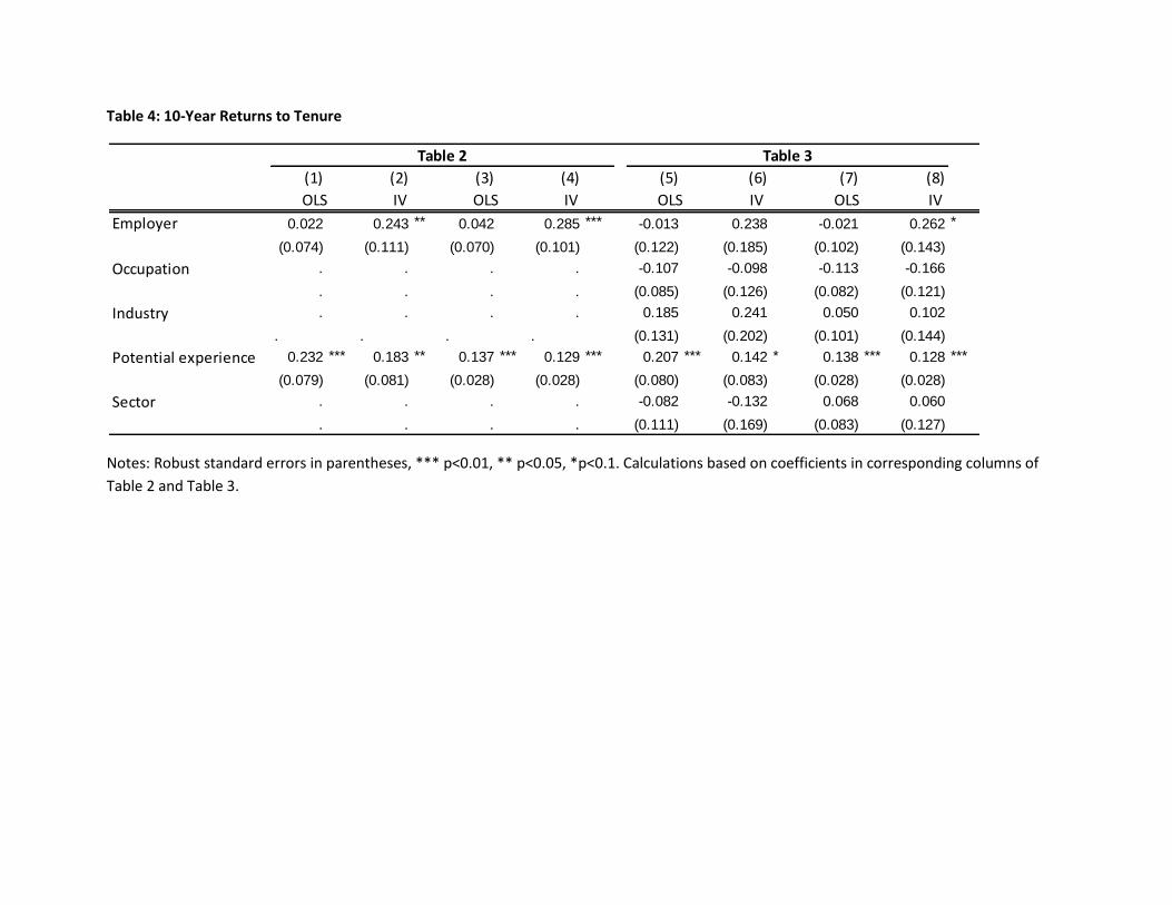
Table 4: 10-Year Returns to Tenure
Notes: Robust standard errors in parentheses, *** p<0.01, ** p<0.05, *p<0.1. Calculations based on coefficients in corresponding columns of
Table 2 and Table 3.
(1) (2) (3) (4) (5) (6) (7) (8)
Employer 0.022 0.243 ** 0.042 0.285 *** -0.013 0.238 -0.021 0.262 *
(0.074) (0.111) (0.070) (0.101) (0.122) (0.185) (0.102) (0.143)
Occupation . . . . -0.107 -0.098 -0.113 -0.166
. . . . (0.085) (0.126) (0.082) (0.121)
Industry . . . . 0.185 0.241 0.050 0.102
. . . . (0.131) (0.202) (0.101) (0.144)
Potential experience 0.232 *** 0.183 ** 0.137 *** 0.129 *** 0.207 *** 0.142 * 0.138 *** 0.128 ***
(0.079) (0.081) (0.028) (0.028) (0.080) (0.083) (0.028) (0.028)
Sector . . . . -0.082 -0.132 0.068 0.060
. . . . (0.111) (0.169) (0.083) (0.127)
OLS IV OLS IV
Table 3
OLS IV OLS IV
Table 2

Table 5: Returns to Tenure by Sector
Notes: Robust standard errors in parentheses, *** p<0.01, ** p<0.05, *p<0.1. Occupation, industry,
province, and year fixed effects are included.
(1) (2)
OLS IV
0.006 0.027*
(0.011) (0.015)
-0.011 -0.013
(0.008) (0.012)
0.004 0.007
(0.010) (0.014)
0.014*** 0.013***
(0.003) (0.003)
Sector tenure 0.025** 0.035**
(0.010) (0.015)
Informal -0.062 0.012
(0.058) (0.063)
Informal x Sector tenure -0.028** -0.043***
(0.011) (0.015)
Old job -0.118** -0.108*
(0.049) (0.056)
Married 0.170*** 0.133***
(0.047) (0.047)
Education 0.100*** 0.099***
(0.009) (0.009)
-0.016 -0.018
rate (0.017) (0.017)
Observations 1,611 1,611
R-squared 0.309 0.302
Province unemployment
Employer tenure
Occupation tenure
Industry tenure
Dependent variable:
Hourly wage
Potential experience

Table 6: 10-Year Returns by Sector
Notes: Robust standard errors in parentheses, *** p<0.01, ** p<0.05, *p<0.1. Calculations based on coefficients in corresponding columns of Table 5.
(1) (2)
OLS IV
Employer -0.063 0.164
(0.101) (0.143)
Occupation -0.109 -0.132
(0.081) (0.121)
Industry 0.038 0.069
(0.100) (0.144)
Potential experience 0.140 *** 0.131 ***
(0.028) (0.028)
Formal 0.248 ** 0.348 **
(0.105) (0.154)
Informal -0.028 -0.083
(0.095) (0.138)

Table 7: Comparison to previous literature Panel A.
Panel B.
Notes: “NS”: Not significant. Panel A presents estimated returns to employer tenure and potential experience. Panel B presents estimated returns to employer, occupation, industry, and sector tenure.
(1) (2) (3) (4) (5) (6) (7) (8)
Marinescu
and Triyana
(2014)
Altonji and
Shakotko
(1987)
Topel
(1991)
Altonji and
Williams
(1997)
Dustmann
and
Pereira
(2005)
Dustmann
and
Pereira
(2005)
Beffy et al
(2006)
Beffy et al
(2006)
Indonesia US US US UK Germany US France
Employer 0.285 0.074 0.246 0.130 .054 NS -0.004NS 0.347 -0.002 NS
Potential experience 0.129 0.364 . 0.372 0.821 0.347 0.246 0.458
(1) (2) (3) (4) (5)
Marinescu
and Triyana
(2014)
Parent
(2000)
Parent
(2000)
Kambourov
and
Manovskii
(2009)
Sullivan
(2010)
10 years NLSY PSID 8-years 5-years
Employer 0.164NS 0.006 NS -0.059
Occupation -0.132NS 0.111 0.133
Industry 0.069NS 0.131 0.093 0.063 0.049
Potential experience 0.131 0.236
Formal Sector 0.348
Informal Sector -0.083NS

Table 8: Returns by Sector Using Alternative Definitions of Informality
Notes: Robust standard errors in parentheses, *** p<0.01, ** p<0.05, *p<0.1. Occupation, industry, province, and year fixed effects are included.
(1) (2) (3) (4) (5) (6) (7) (8)
OLS IV OLS IV OLS IV OLS IV
0.008 0.034** 0.017 0.031* 0.019 0.030* 0.008 -0.003
(0.012) (0.016) (0.013) (0.018) (0.012) (0.017) (0.013) (0.016)
-0.017** -0.015 -0.011 -0.005 -0.012 -0.014 -0.016 -0.014
(0.008) (0.013) (0.008) (0.012) (0.009) (0.013) (0.010) (0.014)
0.008 0.010 0.016 0.013 0.015 0.009 0.001 0.028
(0.011) (0.015) (0.010) (0.015) (0.011) (0.016) (0.014) (0.019)
0.015*** 0.014*** 0.013*** 0.012*** 0.015*** 0.014*** 0.004 0.001
(0.003) (0.003) (0.003) (0.003) (0.003) (0.003) (0.004) (0.004)
0.020* 0.020 -0.007 -0.001 -0.008 0.036 0.034*** 0.026*
(0.011) (0.015) (0.013) (0.019) (0.016) (0.023) (0.012) (0.015)
Informal -0.028 0.039 -0.114* -0.078 -0.124* 0.003 -0.059 -0.042
(0.060) (0.065) (0.062) (0.069) (0.072) (0.076) (0.081) (0.082)
Informal x tenure -0.034*** -0.047*** -0.001 -0.008 -0.002 -0.034* -0.041*** -0.041**
(0.012) (0.015) (0.012) (0.016) (0.014) (0.018) (0.014) (0.018)
Old job -0.132*** -0.118** -0.136*** -0.117** -0.134*** -0.119** -0.161** -0.092
(0.050) (0.057) (0.050) (0.057) (0.051) (0.058) (0.071) (0.077)
Potential experience
Sector tenure
Informal: based on
medical benefits
onlyDependent variable:
Informal: self-
employed and
salaried informal in
same category
Informal: not using
information on
medical benefits
Hourly wage
Employer tenure
Occupation tenure
Industry tenure
Informal: all self-
employed and small
firms

Table 8 (continued)
Notes: Robust standard errors in parentheses, *** p<0.01, ** p<0.05, *p<0.1. Occupation, industry, province, and year fixed effects are included.
(1) (2) (3) (4) (5) (6) (7) (8)
OLS IV OLS IV OLS IV OLS IV
Married 0.158*** 0.122** 0.164*** 0.137*** 0.154*** 0.121** 0.279*** 0.246***
(0.048) (0.049) (0.047) (0.047) (0.049) (0.049) (0.061) (0.061)
0.106*** 0.105*** 0.096*** 0.096*** 0.104*** 0.103*** 0.107*** 0.107***
(0.009) (0.009) (0.008) (0.008) (0.009) (0.009) (0.012) (0.012)
-0.011 -0.012 -0.004 -0.006 -0.008 -0.010 0.002 -0.001
rate (0.017) (0.017) (0.017) (0.017) (0.018) (0.018) (0.021) (0.021)
Observations 1,509 1,509 1,571 1,571 1,522 1,522 942 942
R-squared 0.328 0.320 0.292 0.288 0.313 0.305 0.339 0.334
Province unemployment
Education
Hourly wage
Dependent variable:
Informal: self-
employed and
salaried informal in
Informal: not using
information on
medical benefits
Informal: based on
medical benefits
only
Informal: all self-
employed and small
firms

Table 9: 10-Year Returns Using Alternative Definitions of Informality
Notes: Robust standard errors in parentheses, *** p<0.01, ** p<0.05, *p<0.1.
(1) (2) (3) (4) (5) (6) (7) (8)
OLS IV OLS IV OLS IV OLS IV
Employer -0.055 0.224 0.035 0.197 0.055 0.179 -0.084 -0.119
(0.105) (0.150) (0.118) (0.170) (0.110) (0.165) (0.117) (0.146)
Occupation -0.166 ** -0.151 -0.114 -0.051 -0.124 -0.139 -0.156 -0.144
(0.084) (0.126) (0.083) (0.124) (0.087) (0.131) (0.100) (0.140)
Industry 0.078 0.102 0.156 0.132 0.150 0.086 0.012 0.282
(0.108) (0.152) (0.104) (0.146) (0.111) (0.160) (0.141) (0.187)
Potential experience 0.150 *** 0.138 *** 0.126 *** 0.120 *** 0.149 *** 0.143 *** 0.038 0.013
(0.031) (0.030) (0.028) (0.027) (0.029) (0.029) (0.038) (0.039)
Formal 0.197 * 0.200 -0.066 -0.006 -0.076 0.356 0.342 *** 0.258 *
(0.107) (0.153) (0.134) (0.193) (0.158) (0.232) (0.118) (0.147)
Informal -0.142 -0.265 ** -0.074 -0.082 -0.095 0.018 -0.064 -0.148
(0.098) (0.132) (0.113) (0.157) (0.099) (0.152) (0.123) (0.143)
Informal: self-employed
and salaried informal in
same category
Informal: not using
information on medical
benefits
Informal: based on
medical benefits only
Informal: all self-
employed and small
firms

Figure 1: Transitions out of different formality states
Note: The line “Formal” represents the probability that formal workers become either salaried informal
or self-employed within a given year. The other two lines are defined in a similar fashion.
Source: IFLS, Authors’ calculations.

Data Appendix
Data and documentation for the IFLS can be found at:
http://www.rand.org/labor/FLS/IFLS.html
The IFLS collects data to study a wide range of behaviors and outcomes for the Indonesian population.
The IFLS is based on a sample of households representing about 83% of the Indonesian population living
in 13 of the nation’s 26 provinces in 1993. All of the provinces in the main islands of Java and Bali:
Jakarta, West Java, Central Java, Yogyakarta, and East Java, and Bali. The IFLS includes 4 provinces in
Sumatra: North Sumatra, West Sumatra, South Sumatra, and Lampung. The remaining provinces are
West Nusa Tenggara, South Kalimantan, and South Sulawesi. Other provinces were excluded because of
prohibitive costs. Four surveys have been conducted in 1993, 1997, 2000 and 2007. The first wave
(IFLS1) was administered in 1993 to individuals living in 7,224 households, comprising over 22,000
individuals. The sampling approach in the subsequent waves of the IFLS was to re-contact all original
IFLS1 households with living members the last time they had been contacted, plus split-off households
from other waves. IFLS2 consists of 7,620 households, and it succeeded in re-interviewing 94.4% of IFLS1
households. IFLS3 consists of 10,435 households, it re-contacted 95.3% of IFLS1 households. IFLS4
consists of 13,536 households, it re-contacted 93.6% of IFLS1 households. Nearly 91% of IFLS1
households were interviewed in all waves.
I. Employment types, industry and occupation codes
1. Employment types
IFLS Code Employment type
1 Self employed, no employee
2 Self employed, with unpaid family workers/ temporary workers

3 Self employed, with permanent workers
4 Government
5 Private employee
6 Unpaid family worker
7 Casual worker, agriculture
8 Casual worker, non agriculture
In this paper, we categorize employment type into 4 categories as follows:
IFLS Code Employment type
1 Self-employed
2 Self-employed
3 Self-employed
4 Government
5 Private employee
6 Casual worker
7 Casual worker
8 Casual worker
2. Industry
IFLS Code Industry
1 Agriculture
2 Mining

3 Manufacturing
4 Electricity gas water
5 Construction
6 Wholesale, retail, hotel
7 Transportation, communication
8 Finance, insurance, real estate
9 Community, personal service
10 Other
3. Occupation
IFLS Code Occupation
0X or 1X Professional
2X Administrative/managerial
3X Clerical
4X Sales
5X Service
6X Agriculture
7X Operation & production
8X Transportation operations
9X Blue collar
M or MM Military
S or SS Students

The IFLS originally used 2-digit occupation codes but simplified the codes into 1-digit occupation codes
in waves 3 and 4. More detail on occupation list can be found in appendix A of the IFLS1 documentation
for household questionnaire.
II. Variable Construction
Sample construction
We restrict the sample to respondents who were interviewed in at least two consecutive surveys. We
further restrict the sample to males who ever worked between 1988 and 2007, and lived in an urban
area in at least one round of the survey.
1. Raw variables
Employment type
We use the following variables on the respondent’s primary job from each wave of the survey:
Variable Question
IFLS1 TK24A Which category best describes the work that you do?
IFLS2 TK24A Which category best describes the work that you do?
IFLS3 TK24A Which category best describes the work that you do?
IFLS4 TK24A Which category best describes the work that you do?
For labor force participation in non-survey years, we use the following retrospective variables:
Variable Interval Question
IFLS1 TK33 1988-1992 Which category best describes the work that you did?
IFLS2 TK33 1988-1996 Which category best describes the work that you did?
IFLS3 TK33 1996-1999 Which category best describes the work that you did?
IFLS4 TK33 1999-2007 Which category best describes the work that you did?

Employer tenure
The following questions regarding tenure on the same job are asked retrospectively:
Variable Interval Question
IFLS1 TK29 1988-1992 Was your primary job the same as the job in the year of […]?
IFLS2 TK29 1988-1996 Was your primary job the same as the job in the year of […]?
IFLS3 TK29 1996-1999 Was your primary job the same as the job in the year of […]?
IFLS4 TK30 1999-2007 Where did you work? [Check if same employer as previous year]
Industry
We use the following variables on the respondent’s primary job from each wave of the survey:
Variable Question
IFLS1 TK19a_1 What is manufactured/done at your workplace?
IFLS2 TK20Aind What is manufactured/done at your workplace?
IFLS3 TK19Aa In what field of work is this job?
IFLS4 Tk19ab What is manufactured/done at your workplace?
We use the following retrospective questions for non-survey years:
Variable Interval Question
IFLS1 TK31 1988-1992 What was manufactured/done at your workplace in the year of
[…]?
IFLS2 TK32ind 1988-1996 What was manufactured/done at your workplace in the year of

[…]?
IFLS3 TK31Aa 1996-1999 In what field of work was this job?
IFLS4 TK31A 1999-2007 Interviewer’s note: Circle the appropriate field of work
Occupation
We use the following variables on the respondent’s primary job from each wave of the survey:
Variable Question
IFLS1 Occ12 What are your primary duties at your workplace?
IFLS2 TK20Aocc What are your primary duties at your workplace?
IFLS3 TK20Ab Interviewer’s note: Circle the appropriate code according to
primary duties TK20A
IFLS4 occ07tk2 What are your primary duties at your workplace?
We use the following retrospective questions for non-survey years:
Variable Interval Question
IFLS1 TK32 1988-1992 What were your primary duties in the year of […]?
IFLS2 TK32occ 1988-1996 What were your primary duties in the year of […]?
IFLS3 TK32B 1996-1999 Interviewer’s note: Circle the appropriate code according to
primary duties TK32
IFLS4 Occ07 1999-2007 What were your primary duties in the year of […]?
Other variables:
Primary job characteristics

We use the following variables on the respondent’s primary job from each wave of the survey:
IFLS1 IFLS2 IFLS3 IFLS4
Net salary last month tk25r1_m tk25amt tk25a1 tk25a1
Total monthly income - tk25am - -
Net salary last year tk25r1_y tk25ayt tk25a2 tk25a2
Total annual income - tk25ay - -
Net profit last month tk26r1_m tk26amn tk26amn tk26a1
Gross profit, monthly - tk26amg tk26amg -
Net profit last year tk26r1_y tk26ayn tk26ayn tk26a3
Gross profit, annual - tk26ayg tk26ayg -
Health benefits tk25a1_m tk25ame tk25a3e1 tk25a3e1
Health insurance - - tk25a3e2 tk25a3e2
Health benefits: preferred clinic - - tk25a3e3 tk25a3e3
Number of workers - tk20aa tk20aa tk20aa
Hours last week tk21a tk21a tk21a tk21a
Usual hours worked tk22a tk22a tk22a tk22a
Weeks worked last year tk23a tk23a tk23a tk23a
We use the following retrospective questions for non-survey years:
IFLS1 IFLS2 IFLS3 IFLS4
Monthly income - tk34t tk34 -
Total monthly income - tk34 - -
Monthly profit - tk35n tk35n -
Gross income, monthly - tk35g tk35g -

Hours worked/week - tk36 tk36 -
Weeks worked/year - tk37 tk37 -
Health benefits - tk34e - -
We use the consumer price index (CPI) published in the International Financial Statistics (IFS) to obtain
real income. The IFS calculates CPI based on prices in 17 capital cities, this paper will use 2007 as the
base year. We use real monthly wages, and net monthly profits for self-employed respondents as
income. If monthly income is not available, we use annual wages divided by 12, and annual profits
divided by 12 for self-employed respondents. Hours per year is constructed based on normal hours
worked multiplied by weeks worked. Real hourly wages is constructed using annual income divided by
hours worked. We use log hourly wages in the analysis.
We recode response to the number of workers to match the categories in IFLS4. The range is as follows:
1 to 4 workers, 5 to 19 workers, 20 to 99 workers and more than 100.
Respondent characteristics
Date of birth is asked every round of the survey, however, we find some inconsistencies in the responses
across waves. First we take the mean of the maximum and minimum of the mode of reported birth date
and calculate respondent’s age based on the constructed date of birth. If the difference between the
maximum and minimum of the mode is more than 3 years, but the difference between any two of the
reported dates of birth is less than 1 year, we use these closest dates of birth to calculate the mean of
the birth date.

We define years of education as the maximum of the mode of reported years of education. Potential
experience is defined as current age minus education minus 6. We drop observations with negative
potential experience.
2. Constructing tenure on the job, employment type, industry, and occupation
We reshape the data such that each observation is identified by respondent ID and year, instead of
respondent ID and wave.
Imputations for job characteristics:
If occupation is missing but the industry is agriculture, we impute occupation to be casual worker.
Similarly, if industry is missing but occupation is agriculture, we impute industry as agriculture. In more
than 97% of cases where both occupation and industry are available, where occupation is agriculture,
industry is agriculture, and vice versa.
If respondents report being in the military, we impute the employment type to be government worker.
If respondents report having the same job but some characteristics (industry, occupation, or
employment type) are missing, we assume the characteristics remain the same.
For each of the variables occupation, industry, and employment type, if one of them is missing but the 2
others are the same as in the previous or next year, then we assume that the missing variable also stays
the same. This is not problematic for occupation and industry because in non missing cases the
concordance is more than 98%. For employment type, the concordance is still very high (90%) but not
quite as high.

We set the same job indicator to zero for the first year of work. We also set the same job indicator to
zero if there is a major job characteristics change (a change in occupation is not considered a major
change).
The number of workers is only asked in survey years. If the number of workers does not change within a
job, we use the reported category of firm size to impute firm size for non-survey years. If the number of
workers changed within a job, we use the reported firm size in the survey year as the firm size. In this
case, we assume firm size does not change in between survey years.
We assume health benefits do not change within a job. Health benefits may be insurance, medical
allowance or the availability of a preferred provider. If reported health benefits are inconsistent within
one job, we impute health benefits based on the previous or next year’s reported status.
Tenure variables
We increase tenure on the job so long as the same job indicator is equal to one. If we have more than 3
consecutive years of missing indicator, we set the indicator to missing since we do not know the tenure.
We may be underestimating tenure without imputation.
For tenure on employment type, industry and occupation, we use the user-defined command tsspell7 to
count the spell number and sequence number. This command takes into account the panel structure of
the data. Similarly, if there are 3 or more missing values, we count tenure as missing.
7 http://www.stata.com/support/faqs/data/panel.html

Definitions of informality
Variable med1
Workers with any health benefits are considered formal.
Variable inf1
We define self-employment as informal8. Government workers and those in the military are considered
formal. Casual workers and workers in firms with fewer than 20 workers are considered informal9.
Variable infM
We take the definition based on medical benefits as in med1 and supplement the information with inf1.
Variable infM2
We refine our definition based on infM by separating self-employed workers.
Variable inf2
We refine our definition of informality based on inf1 into informal self-employed, informal not self-
employed, and formal workers.
Variable inf2_big
We refine our definition of informality based on inf2 and assume all firms with fewer than 100 workers
are informal.
8 Although firms with more than workers are required to provide medical benefits, and should be formal, we find
that self-employed people with 10 or more workers report no medical benefits. Thus self-employed workers with
more than 10 workers are still considered informal in this dataset. The results are not sensitive to this difference in
definition. 9 70% of workers in firms with fewer than 20 workers are in firms with 10 or fewer workers.