The solution of high dimensional elliptic PDEs with random...
33
The solution of high dimensional elliptic PDEs with random data Ivan Graham, University of Bath, UK. Joint work with: Frances Kuo, Ian Sloan (New South Wales) Dirk Nuyens (Leuven) Rob Scheichl (Bath) CUHK April 2016
Transcript of The solution of high dimensional elliptic PDEs with random...

The solution of high dimensional elliptic PDEswith random data
Ivan Graham, University of Bath, UK.
Joint work with:
Frances Kuo, Ian Sloan (New South Wales)Dirk Nuyens (Leuven)Rob Scheichl (Bath)
CUHK April 2016

High dimensional Problems: PDE with random data
• Many problems involve PDEs with spatially varying datawhich is subject to uncertainty.
Example: groundwater flow in rock underground.
• Uncertainty enters the PDE through its coefficients. (randomfields). The quantity of interest: is a random number or fieldderived from the PDE solution.
Examples: (i) pressure in medium, (ii) effective permeability,(iii) breakthrough time of a pollution plume .
• Typical Computational Goal: expected value of quantity ofinterest.
This is the Forward problem of uncertainty quantification

Some ingredients
PDE Problem:
−∇.k∇p = f with k(x, ω) = exp(Z(x, ω)), lognormal
Random field Z(x, ω) Gaussian at each xspecified mean (= 0 here ) and (rough) covariance.
no uniform ellipticity, Low regularity,high contrast, high stochastic dimension,
Computational goal: Functionals of p, e.g.
E(p(x, ω)) =
∫Ωp(x, ω)dP(ω) high dimensional
Classical method: Monte-Carlo
• random sampling of Z (how to do it?)• Finite element method for p• convergence O(1/
√N) (N = # samples) + FE Error.

Outline of talk
Part I: Algorithm: circulant embedding with Quasi-Monte Carlo
IGG, Kuo, Nuyens, Scheichl, Sloan JCP 2011
Part II: Rigorous error estimates
IGG, Kuo, Nicholls, Scheichl, Schwab, SloanNumer Math 2014
IGG, Scheichl, UllmannStochastic PDE: Analysis and Computation 2014
IGG, Kuo, Nuyens, Scheichl, Sloan in preparation 2016

Gaussian Random Fields (more generally)
PDE Problem:
−∇.k∇p = f + Boundary conditions k = exp(Z)
Covariance function: (centred) stationary field:
E[Z(x, ·)Z(y, ·)] = ρ(x− y), ρ positive definite
Examples:ρ(x− y) = σ2 exp
(− ‖x− y‖/λ
)“exponential”.
ρ(x− y) = σ2 exp(− ‖x− y‖2/λ
)“Gaussian”.
σ2 = variance , λ = lengthscale
The Matern family: ρ = ρβ, β ∈ [1/2,∞).Limiting cases: exponential (β = 1/2), Gaussian (β =∞).

Gaussian Random Fields (more generally)
Loss of uniform ellipticity and boundedness: for all ε > 0:
min[P(k(x, ·) < ε), P(k(x, ·)) > ε−1)] > 0
Mild smoothness condition on ρ(0):Karhunen-Loeve (KL) Expansion: (a.s. convergence)
Z(x, ω) =
∞∑j=1
√µjξj(x)Yj(ω) Yj ∼ N(0, 1)
(ξj , µj) eigenpairs of covariance operator with kernel ρ(x− y).
Kolmogorov’s theorem: With probability 1,k(x, ω) ∈ Ct(D), with t ∈ [0, β)
In fact, for all q ∈ (1,∞),• k ∈ Lq(Ω, Ct(D)),• and ‖p‖Lq(Ω,H1
0 (D)) ≤ ‖a−1min‖Lq(Ω)‖f‖H−1 (Dirichlet problem).

Non-smooth fields : a typical realization (exponential)
λ - “frequency”: Finite element accuracy requires h ≈ λ/10
σ2 - “amplitude”:
maxx k(x, ω)
minx k(x, ω)∼ exp(σ) high contrast

Mixed FEM (f = 0 mixed BCs)
q + k∇p = 0,∇.q = 0
q.n = 0 on ∂D1
p = g on ∂D2
Mixed formulation (q, p) ∈ H(div, D)× L2(D):∫D k−1q.v −
∫D p∇.v = −
∫∂D2
gv.n ,
−∫D w∇.q = 0 for all (v, w).
h = finite element grid size.
PC = Piecewise constants
Space RT0:qh = a + bx but divergence free =⇒ b = 0 .
Quadrature rule: sample k(x, ω) one point per elementEnough for accuracy:IGG, Scheichl, Ullmann,2015

Mixed FEM (f = 0 mixed BCs)
q + k∇p = 0,∇.q = 0
q.n = 0 on ∂D1
p = g on ∂D2
Mixed formulation (q, p) ∈ H(div, D)× L2(D):
m(q,v) + b(p,v) = G(v) ,b(w,q) = 0 for all (v, w).
h = finite element grid size.
PC = Piecewise constants
Space RT0:qh = a + bx but divergence free =⇒ b = 0 .
Quadrature rule: sample k(x, ω) one point per elementEnough for accuracy:IGG, Scheichl, Ullmann,2015

Mixed FEM (f = 0 mixed BCs)
q + k∇p = 0,∇.q = 0
q.n = 0 on ∂D1
p = g on ∂D2
Mixed approximation (qh, ph) ∈ RT0 × PC on a mesh Th:
m(qh,vh) + b(ph,vh) = G(vh) ,b(wh,qh) = 0 for all (vh, wh)
h = finite element grid size.
PC = Piecewise constants
Space RT0:qh = a+ bx but divergence free =⇒ b = 0 .

Mixed FEM (f = 0 mixed BCs)
q + k∇p = 0,∇.q = 0
q.n = 0 on ∂D1
p = g on ∂D2
Mixed approximation (qh, ph) ∈ RT0 × PC on a mesh Th:
m(qh,vh) + b(ph,vh) = G(vh) ,b(wh,qh) = 0 for all (vh, wh)
h = finite element grid size.
PC = Piecewise constants
Space RT0:qh = a+ bx but divergence free =⇒ b = 0 .
Quadrature rule: sample k(x, ω) one point per elementEnough for accuracy: IGG, Scheichl, Ullmann, 2014

Quantities of Interest - computational cell D = (0, 1)2
p = 1 p = 0
~q.~n = 0
~q.~n = 0
1
• Pressure head p(x, ω), e.g. x = (1/2, 1/2).• Effective permeability
keff(ω) =
∫D q1(x, ω)dx
−∫D ∂p/∂x1(x, ω)dx
=
∫Γout
q1(x, ω) dx

Quantities of Interest - computational cell D = (0, 1)2
p = 1 p = 0
~q.~n = 0
~q.~n = 0
1
0
1
1x1
x2
P = 1
P = 0
~q.~n = 0
~q.~n = 0
release point →•
1
• Pressure head p(x, ω), e.g. x = (1/2, 1/2).• Effective permeability
keff(ω) =
∫D q1(x, ω)dx
−∫D ∂p/∂x1(x, ω)dx
=
∫Γout
q1(x, ω) dx
• Breakthrough time Tout(ω) from q.(Time to reach outflow boundary)
• General format: find E[G(p,q)] - some functional G(p,q).

Sampling by K-L truncation : the effect of lengthscale
Z(x, ω) =
∞∑j=1
√µjξj(x)Yj(ω)
exponential covariance in 1D
log log plot of µj for 1 ≤ j ≤ 500:
100 101 102 103
10−6
10−5
10−4
10−3
10−2
10−1
100
Plateau before decay starts
λ = 1λ = 0.1λ = 0.01
An extreme eigenvalue solverchallenge!

Avoiding KL truncation: discretize first in space
Approximation of E[G(p)] by E[G(ph)] (focus on pressure)
FEM + quadrature requires random vectorZ := Z(xi) at M quadrature points
Covariance Matrix: Ri,j = ρ(xi − xj) M ×M
Seek matrix decomposition:
R = BB> (*)
where B is M × s, s ≥M .
Then (finite “discrete KL” expansion)
Z(ω) = BY (ω), where Y ∼ N(0, 1)s i.i.d.
BecauseE[ZZ>] = E[BYY>B>] = BB> = R
M ∼ h−d and so s very large so (*) expensive(?), but....

Sampling via Circulant Embedding
For
not restrictive︷ ︸︸ ︷uniform grids and stationary fields: R is block Toeplitz
Embed R into C - block circulant s× s (Typically s ∼ (2d)M )
0 0.5 1 1.5 2 2.5 30.2
0.3
0.4
0.5
0.6
0.7
0.8
0.9
1
C =
[R AAT B
]
(Cheap) Factorization: C = FΛFH (by FFT)implies Real Factorization: C = BBT (provided diag(Λ) ≥ 0)
E[G(p)] ≈∫RsF (y)
s∏j=1
φ(yj)dy, F (y) = G(ph(·,y))
=
∫[0,1]s
F (Φ−1s (v))dv =: Is(F ) .
φ(y) = exp(−y2/2)/√
2π, Φ−1s = inv. cum. normal
FEM (h) + high dimensional integration (?)

Integration over [0, 1]s (very large s): QMC methods
∫[0,1]s
f(z) dz ≈ 1
N
N∑k=1
f(z(k))
Monte Carlo methodz(k) random uniformO(N−1/2) convergenceorder of variables irrelevant
Quasi-Monte Carlo methodz(k) deterministicclose to O(N−1) convergenceorder of variables very important
64 random points
••
•
••
•
•
•
•
•
•
•••
•
•• •
•
•
•
•
•
•
•
•
•
•
•
•
•
•
•••
•
•
••
•
•
••
• ••
••
•
••
••
••
•
•
•
•
•
•
••
•
64 Sobol′ points•
•
•
•
•
•
•
••
•
•
•
•
•
•
•
•
•
•
•
•
•
•
••
•
•
•
•
•
•
•
•
•
•
•
•
•
•
••
•
•
•
•
•
•
•
•
•
•
•
•
•
•
••
•
•
•
•
•
•
•
64 lattice points•
•
•
•
•
•
•
•
•
•
•
•
•
•
•
•
•
•
•
•
•
•
•
•
•
•
•
•
•
•
•
•
•
•
•
•
•
•
•
•
•
•
•
•
•
•
•
•
•
•
•
•
•
•
•
•
•
•
•
•
•
•
•
•
1

Numerical Results
Covariance
r(x,y) = σ2 exp(− ‖x− y‖1/λ
).
( ‖ · ‖2 similar).
Case 1 Case 2 Case 3 Case 4 Case 5
σ2 = 1 σ2 = 1 σ2 = 1 σ2 = 3 σ2 = 3λ = 1 λ = 0.3 λ = 0.1 λ = 1 λ = 0.1
FEM: Uniform grid h = 1/m on (0, 1)2, M ∼ m2.
Sampling: circulant embedding via FFT (dimension s ≥ 4M )
High dimensional integration: QMC with N Sobol’ points

Algorithm profile
Time (sec) for N = 1000, CASE 1:
percentages in red, orders in blue
m s Setup InvN FFT AMG TOT33 4.1 (+3) 0.00 1.0 17 0.22 4 4.5 76 5.965 1.7 (+4) 0.01 3.9 17 1.2 5 16.5 75 22
129 6.6 (+4) 0.06 15 16 5.1 6 67 73 92257 2.6 (+5) 0.15 62 16 31 8 290 73 400513 1.0 (+6) 0.6 258 15 145 8 1280 73 1750
m2 m2 m2 m2 logm ∼ m2 ∼ m2
InvN = Inversion of cumulative normal
AMG = Algebraic Multigrid = Fast system solver
One MFE solve with 5132 = 2.6(+5) DOF takes ≈ 1.3 sec
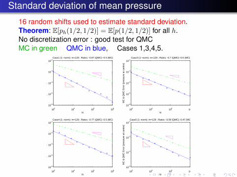
Standard deviation of mean pressure
16 random shifts used to estimate standard deviation.Theorem: E[ph(1/2, 1/2)] = E[p(1/2, 1/2)] for all h.No discretization error : good test for QMCMC in green QMC in blue, Cases 1,3,4,5.
103 104 105 106
10−6
10−5
10−4
10−3
10−2
N
MC
& Q
MC
Err
or (
pres
sure
at c
entr
e)
Case1 (1−norm): m=129 ; Rates:−0.87 (QMC)−0.5 (MC)
103 104 105 10
10−6
10−5
10−4
10−3
10−2
N
MC
& Q
MC
Err
or (
pres
sure
at c
entr
e)
Case3 (1−norm): m=129 ; Rates:−0.7 (QMC)−0.5 (MC)
103 104 105 106
10−6
10−5
10−4
10−3
10−2
N
MC
& Q
MC
Err
or (
pres
sure
at c
entr
e)
Case4 (1−norm): m=129 ; Rates:−0.77 (QMC)−0.5 (MC)
103 104 105 10
10−5
10−4
10−3
10−2
N
MC
& Q
MC
Err
or (
pres
sure
at c
entr
e)Case5 (1−norm): m=129 ; Rates:−0.59 (QMC)−0.47 (MC)

Dimension independence of QMC (and MC)
Standard deviation of mean pressure, Case 4:as m(= 1/h) (and hence s) increasesMC in green QMC in blue
103 104 105 106
10−6
10−5
10−4
10−3
10−2
N
MC
& Q
MC
Err
or (
pres
sure
at c
entr
e)
Case4 (1−norm): m=33 ; Rates:−0.78 (QMC)−0.5 (MC)
103 104 105 10
10−6
10−5
10−4
10−3
10−2
N
MC
& Q
MC
Err
or (
pres
sure
at c
entr
e)
Case4 (1−norm): m=65 ; Rates:−0.74 (QMC)−0.5 (MC)
103 104 105 106
10−6
10−5
10−4
10−3
10−2
N
MC
& Q
MC
Err
or (
pres
sure
at c
entr
e)
Case4 (1−norm): m=129 ; Rates:−0.77 (QMC)−0.5 (MC)
103 104 105 10
10−6
10−5
10−4
10−3
10−2
N
MC
& Q
MC
Err
or (
pres
sure
at c
entr
e)
Case4 (1−norm): m=257 ; Rates:−0.76 (QMC)−0.5 (MC)

Effective permeability keff
discretization error is present.We estimated (by linear regression):h needed to obtain a discretization error < 10−3 (< 2× 10³)N needed to obtain (Q)MC error < 0.5× 10⁻³ (10−3)
(95% confidence)
σ2 λ 1/h N (QMC) N (MC) CPU (QMC) CPU (MC)1 1 17 1.2(+5) 1.9(+7) 3 min 8 h1 0.3 129 3.3(+4) 3.9(+6) 55 min 110 h1 0.1 513 1.2(+4) 5.9(+5) 6.5 h 330 h3 1 33 4.3(+6) 3.6(+8) ∗ 9 h 750 h ∗
3 0.1 513 3.0(+4) 5.8(+5) 20 h 390 h
Smaller λ (lengthscale) needs smaller h but also smaller N .Bigger σ2 (variance) doesn’t affect h but needs larger N
* extrapolated projections.
Strong superiority of QMC in all cases.

Breakthrough time Tout
Here discretization error is more significant.
For Cases 2 and 4 for discr. error < 5 ∗ (10−3) need h = 1/65
For statistical error < 2.5 ∗ 10−3 (95% confidence) need:
Case 2 σ2 = 1, λ = 0.3 NMC = 5.2(+5) NQMC = 1.2(+5)speedup ≈ 4
Case 4 σ2 = 3, λ = 1 NMC = 6.5(+7) NQMC = 4.3(+6)speedup ≈ 15
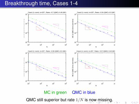
Breakthrough time, Cases 1-4
103 104 105 106
10−4
10−3
10−2
10−1
N
MC
& Q
MC
Err
or (
exit
time)
Case1 (1−norm): m=257 ; Rates:−0.7 (QMC)−0.49 (MC)
103 104 105 106
10−4
10−3
10−2
10−1
N
MC
& Q
MC
Err
or (
exit
time)
Case2 (1−norm): m=257 ; Rates:−0.54 (QMC)−0.5 (MC)
103 104 105 106
10−4
10−3
10−2
10−1
N
MC
& Q
MC
Err
or (
exit
time)
Case3 (1−norm): m=257 ; Rates:−0.58 (QMC)−0.5 (MC)
103 104 105 106
10−3
10−2
10−1
100
N
MC
& Q
MC
Err
or (
exit
time)
Case4 (1−norm): m=257 ; Rates:−0.57 (QMC)−0.45 (MC)
MC in green QMC in blue
QMC still superior but rate 1/N is now missing.

Recent progress on theory (brief)
Primal form (Dirichlet problem)
−∇.k(x, ω)∇p = f on D, p = 0 on ∂D .
• lognormal case: k(x, ω) = exp(Z(x, ω))
• piecewise linear FEM with quadrature: ph
• Linear functional G(p) G(ph)
• Quantity of interest: E[G(p)] Is(F )
where F (y) = G(ph(·,y))
• Randomly shifted lattice rules Qs,N (∆, F )(with N points, defined next slide)
RMS Error e2h,N := E∆
[|Is(F )−Qs,N (∆, F )|2
]

Some QMC Theory (Lattice rules)
Is(F ) :=
∫RsF (y)
∏φ(yj)dy =
∫[0,1]s
F (Φ−1s (z))dz
Qs,N (∆;F ) :=1
N
N∑i=1
F
(Φ−1s
(frac
(i z
N+ ∆
)))generating vector: z ∈ Ns, 1 ≤ zj ≤ N − 1random shift ∆ ∈ [0, 1]s uniformly distributed.
Weighted Sobolev norm: ‖F‖2s,γ :=∑
u⊆1:s1γuJu(F )2
where Ju(F )2 =∫R|u|
(∫Rs−|u|
∂|u|F
∂yu(yu;y1:s\u)
∏j∈1:s\u
φ(yj) dy1:s\u
)2∏j∈u
ψ2j (yj) dyu
γu - controls relative importance of the derivatives
ψj(yj) = exp(−αj |yj |) - controls behaviour as |y| → ∞

QMC Theory...
Theorem (Kuo and Nuyens FoCM 2015) Suppose‖F‖s,γ <∞. Then a generating vector z ∈ Ns can beconstructed (efficiently) so that√
E∆ [|Is(F )−Qs,N (∆, F )|2] ≤ 2
(1
N
)1/2λ
Cs(γ,α, λ)‖F‖s,γ (∗)
for all λ ∈ (1/2, 1]. So the next steps are ...
• Estimate the derivatives ∂|u|ph/∂yu , then derivatives of F .....• Then the norm ‖F‖s,γ .• Choose γu and αj to minimise the RHS of (*).• RHS becomes C(λ)
(1N
)1/(2λ), C(λ) independent of s
provided.... eigenvalues of the circulant satisfy:s∑j=1
(λjs
)λ/(1+λ)
≤ C for all s.
Based on a heuristic for the Matern family ....

Rates for the Matern class
• Dimension independent rate O(
1N−(1−δ)
)δ arbitrarily small, if
ν > 2.
• Dimension independent rate at least O(
1N
)1/2 if ν > 1
Heuristic assumes eigenvalues of the circulant approacheigenvalues of the corresponding periodic covariance integraloperator.
Conclusion:
For Matern parameter ν large enough, combined FE and QMCerror:√
E∆ [|E[G(p)]−Qs,N (∆,G(ph))|2] ≤ C[h2 +N−(1−δ)].
with δ arbitrarily close to 0 independent of dimension s.
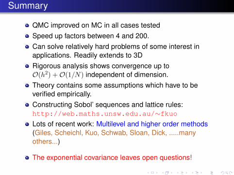
Summary
QMC improved on MC in all cases testedSpeed up factors between 4 and 200.Can solve relatively hard problems of some interest inapplications. Readily extends to 3DRigorous analysis shows convergence up toO(h2) +O(1/N) independent of dimension.Theory contains some assumptions which have to beverified empirically.Constructing Sobol’ sequences and lattice rules:http://web.maths.unsw.edu.au/∼fkuoLots of recent work: Multilevel and higher order methods(Giles, Scheichl, Kuo, Schwab, Sloan, Dick, .....manyothers...)
The exponential covariance leaves open questions!

Dimension independence of QMC (and MC)
Standard deviation of mean pressure, Case 4:as m(= 1/h) (and hence s) increasesMC in green QMC in blue
103 104 105 106
10−6
10−5
10−4
10−3
10−2
N
MC
& Q
MC
Err
or (
pres
sure
at c
entr
e)
Case4 (1−norm): m=33 ; Rates:−0.78 (QMC)−0.5 (MC)
103 104 105 10
10−6
10−5
10−4
10−3
10−2
N
MC
& Q
MC
Err
or (
pres
sure
at c
entr
e)
Case4 (1−norm): m=65 ; Rates:−0.74 (QMC)−0.5 (MC)
103 104 105 106
10−6
10−5
10−4
10−3
10−2
N
MC
& Q
MC
Err
or (
pres
sure
at c
entr
e)
Case4 (1−norm): m=129 ; Rates:−0.77 (QMC)−0.5 (MC)
103 104 105 10
10−6
10−5
10−4
10−3
10−2
N
MC
& Q
MC
Err
or (
pres
sure
at c
entr
e)
Case4 (1−norm): m=257 ; Rates:−0.76 (QMC)−0.5 (MC)