The social cost of rent seeking in Europe · We also investigate the relationship between the size...

European Journal of Political Economy 25 (2009) 280–299

Contents lists available at ScienceDirect

European Journal of Political Economy

j ourna l homepage: www.e lsev ie r.com/ locate /e jpe

The social cost of rent seeking in Europe

Konstantinos Angelopoulos a, Apostolis Philippopoulos a,b,c,⁎, Vanghelis Vassilatos b

a Department of Economics, University of Glasgow, Glasgow, UKb Department of Economics, Athens University of Economics and Business, Athens, Greecec CESifo, Munich, Germany

a r t i c l e i n f o

⁎ Corresponding author. Department of Economics, AE-mail address: [email protected] (A. Philippopoulos)

1 For overviews of rent seeking, see Congleton et al2 The latter is a statistic that the standard real busin3 On the role of the assumption of complete rent di

0176-2680/$ – see front matter © 2009 Elsevier B.V.doi:10.1016/j.ejpoleco.2009.06.001

a b s t r a c t

Article history:Received 1 July 2008Received in revised form 1 June 2009Accepted 1 June 2009Available online 6 June 2009

Direct measurement of the social cost of rent seeking is impeded by non-observable and non-reported activities. We use a dynamic stochastic general equilibrium model to compute thesocial cost of rent seeking in Europe. Our estimate is based on competition among interestgroups for privileges provided by governments, including income transfers, subsidies, andpreferential tax treatment. The model, which is calibrated to the euro area as a whole and alsoto individual euro member countries for 1980–2003, performs well vis-à-vis the data. We findthat significant proportions of GDP are extracted as rents available to be sought by rent seekers.

© 2009 Elsevier B.V. All rights reserved.

JEL classification:E62E32O17

Keywords:Rent seekingRent extractionPrivilegeTaxationPublic spending

1. Introduction

The social costs of rent seeking are incurred when resources are unproductively used in quest of privileges from government.1 Theprivileges sought involve preferential tax treatment and benefit from public spending, which offer private gain from common-poolstate coffers (Park et al., 2005). The non-observed and non-reported activities involved in creating, extracting, and contesting rents areimpediments to direct empirical estimation of the social cost of rent seeking. We therefore apply computational methods to suggestvaluesof social loss fromrent seeking inEurope.Weuseadynamic stochastic general equilibriummodel calibrated to theeuro area andto individual EU-12 countries (the initial group of twelve European countries that adopted the euro by 2001) over the period 1980–2003. Themodel also suggestsmacroeconomic implications;we are not aware of a previous calibration or estimation that explores thelink between rent seeking and themacro-economy in amicro-founded dynamic general equilibriummodel. Themodel performswellvis-à-vis the data by matching key statistical properties (volatility, persistence and co-movement) of the business cycle in the euroarea. The model also fares better than the same model without rent seeking in terms of volatility in hours worked.2

For the euro area as a whole, our model suggests that some 18% of collected tax revenues are extracted as rents, whichcorresponds to public spending and tax privileges equal to 7% of output produced. If we assume complete rent dissipation, thesevalues are also social costs of rent seeking.3 At the individual country level, Ireland and the Netherlands exhibit essentially zero rentextraction and rent seeking, followed by Finland. Greece, Portugal and Italy exhibit the highest rent extraction and rent seeking,followed by post-reunification Germany.

thens University of Economics and Business, Athens, Greece. Tel.: +30 210 8203357; fax:+30 210 8203301.. (2008a) and Hillman (2009, chapter 2).ess cycle model finds difficult to match (King and Rebelo, 1999; Hall, 1999).ssipation in inferring the social cost of rent seeking, see Hillman (2009, chapter 2).

All rights reserved.

.

mailto:[email protected]

http://dx.doi.org/10.1016/j.ejpoleco.2009.06.001

http://www.sciencedirect.com/science/journal/01762680

281K. Angelopoulos et al. / European Journal of Political Economy 25 (2009) 280–299

We also investigate the relationship between the size of the government and rent seeking activities. The latter activitiesdepend on most exogenous variables and calibrated parameters, of which the size of the government is one. For instance,despite high tax rates and large public sectors, Finland and the Netherlands exhibit low rent seeking due to their good“institutional quality”, as measured by a calibrated technology parameter that converts individual rent-seeking effort into rentextraction. Greece and Portugal have small government spending but exhibit high rent extraction and rent seeking because ofpoor institutional quality. Rent seeking in Germany is driven mainly by a large government size: its institutions are around theEU quality average.

We also quantify the potential welfare gains from improvements in institutional quality whereby the same rent-seeking effortresults in less actual rent extraction because of better andmore strictly enforced laws. Our results suggest that small improvementsin institutional quality can result in substantial welfare gains.

Section 2 presents the model. Section 3 discusses the methodology and data problems. The quantitative study is described inSections 4, 5 and 6. Welfare exercises are reported in Section 7. Extensions are discussed in Section 8. Section 9 briefly summarizesthe conclusions.

2. Theoretical model

2.1. Description of the model

We build upon Park et al. (2005). There is a large number of identical households and (for simplicity) an equal number ofidentical firms. Households own capital and labour, which they supply to firms, and engage in rent-seeking competition for fiscalprivileges.4 A household chooses consumption, leisure and saving, and the allocation of non-leisure time between productiveworkand rent-seeking activity. Firms produce a homogenous product using capital, labour, and public infrastructure. The governmentuses tax revenues and issues bonds to finance: (1) public consumption (which provides direct utility to households), (2) publicinvestment (which augments the stock of public infrastructure providing production externalities to firms), (3) a uniform lump-sum transfer to each household, and (4) fiscal privileges to rent seekers.

2.2. Examples of rent seeking from state coffers

We distinguish between two categories of rent seeking that need not be mutually exclusive.The first category consists of privileged transfers, subsidies and tax treatments: these are direct transfers either in cash

(targeted subsidies and other benefits) or in-kind (private use of public assets such as state cars, extra health services and childbenefits, etc.) as well as indirect transfers (policies that increase the demand for an interest group's services, etc). There are alsopolicies that reduce tax burdens (tax exemptions and loopholes favoring special interests) combined with an increase in theaverage tax rate to compensate for the lost revenue. There are also illegal forms of rent seeking (such as tax evasion, theft of fundsfor public programs, use of fake documents to obtain privileged treatment, etc.).

The second category of rent seeking consists of privileged regulation and legislation that reduce competition(government-created barriers to entry, trade restrictions and agricultural price supports), disguised transfers (a publicroad may increase the value of real estate, etc), and privileged avoidance of regulation. Again, there are legal and illegalforms.

Our model is conceptually consistent with both categories of rent seeking. The formal model however focuses on the firsttype.5

2.3. Households

In each period t there are Nt identical households indexed by the superscript h, where h=1,2,…, Nt. The population size Nt

evolves at a constant rate γn≥1 so that Nt+1=γnNt, where N0N0 is given. The expected lifetime utility of household h is:

4 Weat what

5 Our

E0X∞t=0

β4tu Cht + ψGc

t ; Lht

� �ð1Þ

E0 denotes rational expectations conditional on the information set available at time zero, 0bβ*b1 is a time discount factor,
whereCth is h's private consumption at time t, Gt
c is average (per household) public consumption goods and services provided by thegovernment at t, and Lt

h is h's leisure time at t. Thus, public consumption of goods and services influences private utility throughthe value of the parameter Ψ.

focus on the demand side of rent seeking. The supply side of fiscal favors (why and how government officials and voters decide to offer these favors, andprice) is not modeled. See Section 8 below.list of privileged rents is not exhaustive: for other examples, see for example Tanzi (1998) and Hillman (2009, chapter 2).

282 K. Angelopoulos et al. / European Journal of Political Economy 25 (2009) 280–299

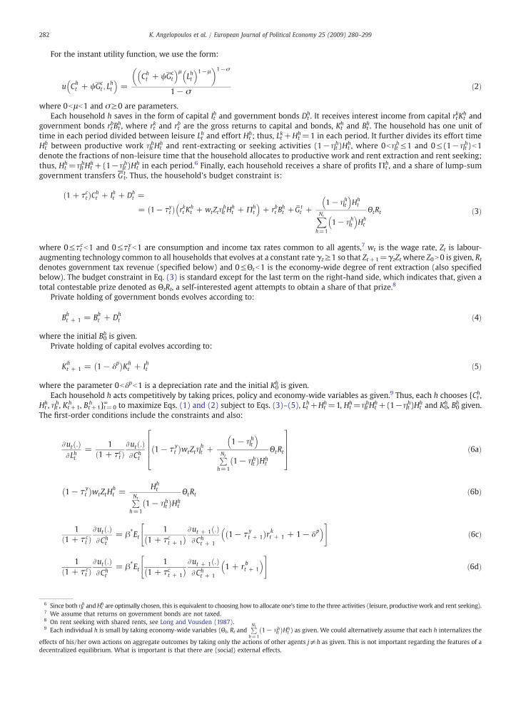
For the instant utility function, we use the form:

6 Sinc7 We8 On9 Eac

effectsdecentr

u Cht + ψGc

t ; Lht

� �=

Cht + ψGc

t

� �μLht� �1−μ

� �1−σ

1− σð2Þ

0bμb1 and σ≥0 are parameters.
whereEach household h saves in the form of capital Ith and government bonds Dt
h. It receives interest income from capital rtkKth and

government bonds rtbBt

h, where rtk and rt

b are the gross returns to capital and bonds, Kth and Bt

h. The household has one unit oftime in each period divided between leisure Lt

h and effort Hth; thus, Ltk+Ht

h=1 in each period. It further divides its effort timeHth between productive work ηthHt

h and rent-extracting or seeking activities (1−ηth)Hth, where 0bηth≤1 and 0≤(1−ηth)b1

denote the fractions of non-leisure time that the household allocates to productive work and rent extraction and rent seeking;thus, Ht

h=ηthHth+(1−ηth)Ht

h in each period.6 Finally, each household receives a share of profits Πth, and a share of lump-sum

government transfers Gtt. Thus, the household's budget constraint is:

1 + τct� �

Cht + Iht + Dh

t =

= 1− τyt� �

rkt Kht + wtZtη

ht H

ht + Πh

t

� �+ rbt B

ht +G t

t +1− ηht� �

Hht

XNt

h=1

1− ηht� �

Hht

ΘtRt ð3Þ

0≤τtcb1 and 0≤τtyb1 are consumption and income tax rates common to all agents,7 wt is the wage rate, Zt is labour-
whereaugmenting technology common to all households that evolves at a constant rate γz≥1 so that Zt+1=γzZt where Z0N0 is given, Rtdenotes government tax revenue (specified below) and 0≤Θtb1 is the economy-wide degree of rent extraction (also specifiedbelow). The budget constraint in Eq. (3) is standard except for the last term on the right-hand side, which indicates that, given atotal contestable prize denoted as ΘtRt, a self-interested agent attempts to obtain a share of that prize.8
Private holding of government bonds evolves according to:

Bht + 1 = Bh

t + Dht ð4Þ

the initial B0h is given.
wherePrivate holding of capital evolves according to:
Kht + 1 = 1− δp

� �Kht + Iht ð5Þ

the parameter 0bδpb1 is a depreciation rate and the initial K0h is given.
where
Each household h acts competitively by taking prices, policy and economy-wide variables as given.9 Thus, each h chooses {Cth,Hth, ηth, Kt+1

h , Bt+1h }t=0

∞ to maximize Eqs. (1) and (2) subject to Eqs. (3)–(5), Lth+Hth=1, Ht

h=ηthHth+(1−ηth)Ht

h and K0h, B0h given.

The first-order conditions include the constraints and also:

Aut :ð ÞALht

=1

1 + τctð ÞAut :ð ÞACh

t

1− τ yt

� �wtZtη

ht +

1− ηht� �

PNt

h=11− ηht� �

Hht

ΘtRt

26664

37775 ð6aÞ

1− τ yt

� �wtZtH

ht =

HhtPNt

h=11− ηht� �

Hht

ΘtRt ð6bÞ

11 + τ c

tð ÞAut :ð ÞACh

t

= β4Et1

1 + τct + 1

� �Aut + 1 :ð ÞACh

t + 1

1− τ yt + 1

� �r kt + 1 + 1− δp

� �" #ð6cÞ

11 + τ c

tð ÞAut :ð ÞACh

t

= β4Et1

1 + τct + 1

� �Aut + 1 :ð ÞACh

t + 1

1 + r bt + 1

� �" #ð6dÞ

e both ηth andHth are optimally chosen, this is equivalent to choosing how to allocate one's time to the three activities (leisure, productivework and rent seeking).

assume that returns on government bonds are not taxed.rent seeking with shared rents, see Long and Vousden (1987).h individual h is small by taking economy-wide variables (Θt, Rt and

PNt

h=11− ηht� �

Hht ) as given. We could alternatively assume that each h internalizes the

of his/her own actions on aggregate outcomes by taking only the actions of other agents j≠h as given. This is not important regarding the features of aalized equilibrium. What is important is that there are (social) external effects.


Condition (6a) is the optimality condition with respect to effort time Hth and equates the marginal value of leisure to the after-

tax return to effort. Condition (6b) is the optimality conditionwith respect to the fraction of non-leisure time allocated towork vis-à-vis rent extraction and rent seeking ηth; in equilibrium, the return to work and the return to rent extraction and rent seeking areequal. Eqs. (6c) and (6d), are standard Euler equations for Kt+1

h and Bt+1h . The optimality conditions are completed by the

transversality conditions for the two assets, namely limtY∞

βTtE0Aut :ð ÞACh

t

Kht + 1 = 0 and lim

tY∞βTtE0

Aut :ð ÞACh

t

Bht + 1 = 0.

2.4. Firms

There are as many firms as households. Identical firms are indexed by the superscript f, where f=1,2,…, Nt. Each firm producesa homogeneous product Yt

f by choosing private capital Ktf and private labor Qt

f and by using average (per firm) public capital Ktg. Its

production function is:

subjec

where

10 Wecalibratthat the

Yft = At Kf

t

� �αQft

� �eKgt

� �1−α− e ð7Þ

AtN0 is stochastic total productivity (see below for its law of motion) and 0, α, and εb1 are parameters (see Lansing, 1998,
wherefor a similar production function).10
Each firm f acts competitively by taking prices, policy and economy-wide variables as given. Thus, each f chooses Ktf and Qtf to

maximize a series of static profit problems:

Π ft = Y f

t − rkt Kft − wtQ

ft ð8Þ

t to Eq. (7). The first-order conditions are:

αYft

Kft

= rkt ð9aÞ

eYft

Q ft

= wt : ð9bÞ

2.5. Government

The government collects tax revenue Rt by taxing consumption and income at the rates 0≤τtcb1 and 0≤τtyb1. Rent seekersextract ΘtRt, where the economy-wide fraction of rent seeking 0≤Θtb1 is modelled below. Then the government uses theremaining tax revenue (1−Θt)Rt and issues new bonds, Bt+1 to finance public consumption Gt

c, public investment Gti, and lump-

sum transfers Gtt. Thus, the government budget constraint at t is:

Gct + Gi

t + Gtt + 1 + rbt

� �Bt = Bt + 1 + 1− Θtð ÞRt ð10Þ

RtuτctPNt

h=1Cht + τyt rkt

PNt

h=1Kht + wtZt

PNt

h=1ηht H

ht +

PNt

h=1Πh

t

!is tax revenue. Notice that ΘtRt can be either government
where
revenue taken away (i.e. privileged tax treatments) and as extra benefits recorded as expenditure (i.e. privileged spendingsubsidies).

Public investment Gti is used to augment the stock of public capital, whose motion is:

Kgt + 1 = 1− δg

� �Kgt + Gi

t ð11Þ

0bδgb1 is a depreciation rate and initial K0g is given.

2.6. Exogenous stochastic variables and policy instruments

The exogenous stochastic variables include the aggregate productivity At and five policy instruments Gtc, Gt

i, Gtt, τty, τtc. We

assume that productivity and policy instruments (in rates) follow stochastic AR(1) processes (see Baxter and King, 1993).

include public investment, and hence public capital, because we wish to be as close as possible to the data concerning public finance. This helps us toe the model more accurately (see also Baxter and King, 1993; Lansing, 1998). Nevertheless, we report in Section 4.4 below outcomes when ε=1–α sore is no productive role for public expenditure.


Specifically, we define sctuGct

Yt, situ

Git

Yt, sttu

Gtt

Ytto be the three categories of government spending as shares of output. We assume that

At, stc, sti, stt, τty, τtc follow univariate stochastic AR(1) processes:

whereεta, εtg,

11 We12 Thu

Bt =PNh=

ln At + 1 = 1− ρað Þln A0 + ρa ln At + eat + 1 ð12aÞ

ln sct + 1 = 1− ρg

� �ln sc0 + ρg ln sct + e

gt + 1 ð12bÞ

ln sit + 1 = 1− ρið Þln si0 + ρi ln sit + eit + 1 ð12cÞ

ln stt + 1 = 1− ρtð Þln st0 + ρt ln stt + ett + 1 ð12dÞ

ln τyt + 1 = 1− ρy

� �ln τy0 + ρy ln τyt + e

yt + 1 ð12eÞ

ln τct + 1 = 1− ρcð Þln τc0 + ρc ln τct + ect + 1 ð12fÞ

A0, s0c , s0i , s0t , τ0y, τ0c, are means of the stochastic processes; ρa, ρg, ρi, ρt, ρy, ρc are first-order autocorrelation coefficients; andεti, εtt, εty, εtc, are i.i.d. shocks.

2.7. Economy-wide rent extraction

To close the model, we specify the economy-wide degree of rent extraction (0≤Θtb1). This can depend on many variables.Here, following for instance Zak and Knack (2001), Mauro (2004) and Park et al. (2005), we simply assume that Θt increases with

per capita rent-seeking activities,

PNth=1

1 − ηhtð ÞHht

Nt(see Section 7 for a richer specification). Using for simplicity a linear specification, we

assume:11

Θt = θ0

PNt

h=11− ηht� �

Hht

Ntð13Þ

θ0≥0 is a technology parameter that translates rent-seeking effort into rent extraction. Higher values of θ0 indicate a more
where“efficient” rent-seeking technology, through permissive legal systems and permissible corruption, etc. Thus, θ0 is a measure ofinstitutional quality, with higher values indicating worse institutions. Note that our model distinguishes between rent creation(government income, Rt), rent seeking efforts (each person h allocates (1−ηth)Ht
h to rent seeking) and actual rent extraction in theeconomy (ΘtRt).

2.8. Decentralized Competitive Equilibrium (DCE)

In a Decentralized Competitive Equilibrium (DCE): (i) Each individual household and each individual firm maximizerespectively their own utility and profit by taking as given market prices, government policy and economy-wide outcomes.(ii) arkets clear through price flexibility.12 (iii) The government budget constraint is satisfied. This equilibrium holds for anyfeasible policy. We solve for a symmetric DCE. Equilibrium quantities will be denoted by letters without the superscripts h (whichwas used to indicate quantities chosen by households) and f (which was used to indicate quantities chosen by firms). The DCE isgiven by Eqs. (1)–(13). Looking ahead at the long run where all components of the national income identity grow at the sameconstant rate (the so-called balanced-growth rate), we transform these components in per capita and efficient unit terms to makethem stationary. Thus, for any economy-wide variable Xt, Xt≡(Yt, Ct, Kt, Bt, Kt

g, Gtc, Gt

i, Gtt), we define xtu Xt

NtZt. We also define htu Ht

Ntto

be per capita non-leisure time. It is then straightforward to show that Eqs. (1)–(13) imply the following stationary DCE:

ct + ψsct yt� �

1− htð Þ =μ

1 + τctð Þ 1− μð Þ θ0 τct ct + τyt yt� � ð14aÞ

ηthtθ0 =e 1− τyt� �

ytτct ct + τyt yt� � ð14bÞ

could instead use a non-linear form like a Cobb–Douglas function. This would not affect our main results.

s, in each time period,PNt

f =1Kft =

PNt

h=1Kht in the capital market,

PNt

f =1Qf

t = ZtPNt

h=1ηht H

ht in the labor market,

PNt

f =1Πf

t =PNt

h=1Πh

t in the dividend market, andt

1Bht in the bond market.

whereproduecono

Table 1Calibrat

Parame

δp

δg

A0

μσγn

Ψρaσa

βαεθ0γz

s0i

s(d)0t

τ0y

τ0c

ρgρiρtσg

σi

σt


ct + ψsct yt� �μ 1−htð Þ1−μ� �1−σ

1 + τctð Þ ct + ψsct ytð Þ =

= βEt

ct + 1 + ψsct + 1yt + 1� �μ 1−ht + 1

� �1−μ� �1−σ

1− τyt + 1

� �αyt + 1

kt + 1+ 1− δp

� 1 + τct + 1

� �ct + 1 + ψsct + 1yt + 1� �

2664

3775

ð14cÞ

ct + ψsct yt� �μ 1−htð Þ1−μ� �1−σ

1 + τctð Þ ct + ψsct ytð Þ = βEtct + 1 + ψsct + 1yt + 1� �μ 1−ht + 1

� �1−μ� �1−σ

1 + rbt + 1

� �1 + τct + 1

� �ct + 1 + ψsct + 1yt + 1� �

264

375 ð14dÞ

1− sct − sit� �

yt = ct + it ð14eÞ

yt = Atkαt ηtht� �ekg1−α− e

t ð14fÞ

γnγzkgt + 1 = 1− δg

� �kgt + sityt ð14gÞ

γnγzkt + 1 = 1− δp� �

kt + it ð14hÞ

γnγzbt + 1 − 1 + rbt� �

bt = sct + sit + stt� �

yt − 1− θ0 1− ηt� �

ht� �

τct ct + τyt yt� � ð14iÞ

β≡β*γ zµ(1−σ)−1. We thus have nine equations in the paths of it, ct, yt, rtb, ηt, ht, bt+1, kt+1

g , kt+1. This gives the paths ofctivity At and the independent policy instruments, stc, sti, stt, τty, τtc, whose motion is defined in Eqs. (12a–f) above. Our modelmy in the long run is presented in Appendix A where variables without time subscripts denote long-run values.

3. Taking the model to the data

Our model includes variables that – although clearly identifiable from a theoretical point of view – are difficult or impossible toobserve and measure. Prime examples are the fraction of effort time allocated to productive work relative to rent seeking 0bηt≤1and hours devoted to productivework ηtht. To address themeasurement problem, we assume that effort at rent seeking takes placewhile at work. This reflects the view that trade union and lobbying activities are at the expense of hours of productive work. We

ion.

ter or variable Description Value Source

Private capital depreciation rate (quarterly) 0.0250 SetPublic capital depreciation rate (quarterly) 0.0250 SetLong-run aggregate productivity 1.0000 SetConsumption weight in utility function 0.3713 SetCurvature parameter in utility function 2 SetGrowth rate of population 1 SetSubstitutability between private and public consumption in utility 0 SetPersistence parameter of At 0.9900 SetStandard deviation of the innovation εta 0.0063 SetTime discount factor 0.9912 CalibratedPrivate capital share in production 0.2503 CalibratedLabor share in production 0.7202 CalibratedExtraction technology parameter 4.7593 CalibratedGrowth rate of labor-augmenting technology 1.0088 Data averageGovernment investment to output ratio 0.0295 Data averageGovernment transfers to output ratio 0.2026 Data averageAverage income tax rate 0.2800 Data averageAverage consumption tax rate 0.1700 Data averagePersistence parameter of stc 0.9933 EstimatedPersistence parameter of sti 0.8477 EstimatedPersistence parameter of stt 0.9871 EstimatedStandard deviation of the innovation εtg 0.0121 EstimatedStandard deviation of the innovation εti 0.0073 EstimatedStandard deviation of the innovation εtt 0.0071 Estimated

13 See Burnside and Eichenbaum (1996) for a similar approach in an estimated RBC model with several unobservable variables because of factor hoarding.14 We are grateful to Harald Uhlig for pointing out this problem. This implies that we may have a double-counting problem, in the government budgeconstraint in Eq. (10) if we use the available data on government spending to measure Gt

c, Gti and Gt

t, and in addition allow for rent seeking (θtRt). Since we usedata on collected tax revenue, a similar problem does not arise in the case where rent seeking takes the form of tax favors.15 Total employment is equal to the employment rate multiplied by the labour force. On the assumption that there are 7×14 h per week and the averageworking week is 40 h, labour hours are obtained if we multiply total employment by the factor 40/(7×14). Note that this is not necessary for individuacountries where data are available (see below).

Table 2Data averages and long-run solution.

Variable Description Data average Long-run solution

c/y Consumption-to-output ratio 0.5694 0.6348i/y Private investment to output ratio 0.18 0.18h Hours at work 0.3713 0.3188η Fraction of hours at work allocated to productive work Na 0.8809nh Hours of productive work Na 0.2809Θ Share of tax revenue extracted by rent seekers Na 0.1807Θr/gt Transfers due to rent seeking as a share of total transfers Na 0.3460Θr/y Transfers due to rent seeking as a share of output Na 0.0701k/y Private capital to output ratio Na 5.3169kg/y Public capital to output ratio Na 0.8714rb Return to bonds (quarterly) 0.0089 0.0089b/y Public debt-to-output ratio (quarterly) 2.3288 2.4s0c Government consumption-to-output ratio 0.2041 0.1557

Notes: Na denotes not available.


thus distinguish hours at work ht, which is measurable, from hours of productive work ηtht, which is unobservable. Although we donot have data on ηt, we can use the condition (14b) to deduce ηt given time-series for yt, ct, τty, τtc, ht, and values for the model'sstructural parameters, θ0 and ε, where these parameter values are calibrated below (for instance, all variables in Eq. (A.i) inAppendix A are observable so that this equation can give a calibrated value for θ0, the extraction technology parameter).13 This inturn gives the economy-wide degree of extraction, Θt, via Eq. (13).

Also, public finance data do not distinguish between government spending arising from rent-seeking activities and governmentspending independent of such activities. Because the data contain both types, Gt

t (i.e. transfers net of rent seeking) isunmeasured.14 However, since we have assumed that spending favors take the form of transfers, this means that only thegovernment budget constraint (A.vi) is affected, and this can be rewritten as Eq. (A.vi′) which includes observables only (seeAppendix A for details).

To use the theoretical framework for quantitative results, we calibrate the model by following a three-step procedure thatfollows the tradition in the literature. First, we assign numerical values to the parameters of the model. This requires setting asmany numbers as possible according to balanced-growth conditions, i.e. our model economy mimics the actual economy in thelong run. As long-run values of variables, we use the average values of the time-series in the data. Second, we linearly approximatethe equilibrium conditions around the resulting long-run solution. Third, we study whether the linearized model can generatefluctuations that are associated with the business cycle. To do so, we simulate our model economy and compare key second-moment properties of the series generated by the model to those of the actual data (where we use the Hodrick–Prescott filter toobtain the cyclical component of the series). We also present impulse response functions.

4. Calibration and long run of the euro area

We first calibrate themodel to the euro zone area as awhole. Our data source is the updated AWMdataset constructed by Faganet al. (2001). Data are quarterly and cover the period 1980:1–2003:4. Table 1 reports the calibrated parameter values and theaverage values of exogenous variables (time-series) in the data. Table 2, column 1, reports the average values of endogenousvariables (time-series) in the data, while the long-run solution of the model is in column 2.

4.1. Data averages

The average values of tax rates in the data are in Table 1. The income tax rate τ0y is obtained as the ratio of the collected incometax revenue to GDP. The consumption tax rate τ0c is the ratio of collected indirect tax revenue over private consumption. Dataaverages of the three government spending-to-output ratios are also in Table 1. Table 2, column 1, reports the average values of c/y,i/y, h and b/y in the data. The average quarterly real interest rate on public debt rb is 0.0089, which implies an annual value of0.036. Since data on hours at work are not available for the euro zone area as awhole, the series of ht is computed as in for instanceCorreia et al. (1995) and its average value is found to be h=0.3713.15

t

l

Table 3Comparative statics and long-run solution.


16 The AWM database does not report data on private and public capital. We choose to calculate the two long-run capital output ratios rather than to constructhe respective series by using for instance a perpetual inventory method.

Table 4Rent seeking results in individual euro countries.

Country θ0 η Θ Θr/gt Θr/y τ0y τ0c gt/r gt/y ICRG

Austria 4.5 (2) 0.85 (6) 0.21 (7) 0.28 (5) 0.08 (6) 0.28 0.18 0.78 0.3 47.22 (5)Belgium 4.9 (3) 0.84 (7) 0.20 (6) 0.36 (7) 0.09 (7) 0.32 0.16 0.57 0.23 47.46 (4)Finland 4.45 (1) 0.97 (3) 0.03 (3) 0.05 (3) 0.01 (3) 0.3 0.18 0.67 0.26 48.76 (3)France 5.47 (5) 0.92 (4) 0.1 (4) 0.16 (4) 0.04 (4) 0.28 0.19 0.65 0.25 46.62 (6)Germany 5.6 (6) 0.82 (8) 0.26 (8) 0.41 (8) 0.1 (8) 0.29 0.18 0.64 0.25 48.92 (2)Greece 7.36 (10) 0.8 (10) 0.53 (11) 0.77 (11) 0.16 (11) 0.19 0.14 0.7 0.20 34.36 (11)Ireland 6.5 (8) No RS (1) No RS (1) No RS (1) No RS (1) 0.2 0.14 0.67 0.18 44.37 (7)Italy 5.66 (7) 0.8 (10) 0.32 (9) 0.56 (9) 0.12 (9) 0.28 0.16 0.58 0.22 40.90 (8)Netherlands 5.36 (4) No RS (1) No RS (1) No RS (1) No RS (1) 0.3 0.14 0.64 0.24 49.40 (1)Portugal 7.58 (11) 0.81 (9) 0.52 (10) 0.71 (10) 0.13 (10) 0.18 0.11 0.74 0.18 40.13 (10)Spain 6.56 (9) 0.9 (5) 0.19 (5) 0.28 (5) 0.05 (5) 0.22 0.1 0.69 0.19 40.4 (9)

Notes:1. θ0 is a calibrated value, while η, Θ, Θr/gt and Θr/y are long-run solutions. τ0c , τ0y, gt/r and gt/y are data averages from OECD Economic Outlook. See the text fordefinitions.2. The ICRG index is based on annual values for indicators of the quality of governance, corruption and violation of property rights over the period 1982–1997. It hasbeen constructed by Stephen Knack and the IRIS Center, University of Maryland, frommonthly ICRG data provided by Political Risk Services. This index takes valueswithin the range 0–50, with higher values indicating better institutional quality. Our reported numbers are the averages over 1982–1997. Knack and Keefer (1995)provide a detailed discussion of this index.3. Numbers in parentheses denote the ranking of countries in each column. A smaller number indicates less rent seeking.4. The correlation between ICRG and {θ0, η, Θ, Θr/gt, Θr/y} is {−0.81, 0.49, −0.78, −0.77, −0.66}.


4.2. Calibration

Some parameter values in Table 1 are set on the basis of a priori information. Following the usual practice, the curvatureparameter in the utility function σ is set equal to 2. The parameter ψ, which measures the degree of substitutability/complementarity between private and public consumption in the utility function, is set equal to 0; as Christiano and Eichenbaum(1992) explain, this means that government consumption is equivalent to a resource drain in the macro-economy. Since quarterlypopulation data for the euro zone as a whole are not available, we assume away population growth, γn=1. The private and publiccapital depreciation rates, and δg, are both set equal to 0.025 (implying 0.10 annually), which are the values also used by Smets andWouters (2003). The exponent of public capital in the production function (1−α−ε) is set equal to 0.0295, which is the averagepublic investment to output ratio (s0i ) in the data (Baxter and King,1993, do the same for the US). Following Kydland (1995), we setμ (the weight given to consumption relative to leisure in the utility function) equal to the average value of ht (see above). Both Z0(the initial level of technical progress) and A0 (the level of long-run aggregate productivity) are scale parameters and arenormalized to one (King and Rebelo,1999). The growth rate of the exogenous labor-augmenting technology, is 1.0088, which is theaverage GDP growth rate of the Euro zone member countries during 1960–2003.

The remaining parameters are chosen to match the data averages. The time preference rate β is calibrated from Eq. (A.iii). Thecapital share α is calibrated from Eq. (A.ii). Given the values of α=0.2503 and (1−α−ε)=0.0295, the labor share is ε=0.7202.The value of θ0 (the extraction technology parameter) is calibrated from Eq. (A.i) to give θ0=4.7593. As stressed above, thesecalibrated parameter values do not require data on η. We also report that Eqs. (A.ix) and (A.vii) imply respectively k/y=5.3169 andkg/y=0.8714, which are private and public capital stocks as shares of output.16 An implied value of η can follow from Eqs. (A.viii)and is found to be 0.78.

For the simulations below, we also need to specify the parameters (autoregressive coefficients and variances) of the stochasticexogenous processes in Eqs. (12a)–(12f). The coefficients ρg, ρi, ρt and the associated standard deviations,σg,σi,σt, in Eqs. (12b)–(12d)are estimated via OLS from their respective AR(1) processes. Concerning Eq. (12a), we follow the usual practice by choosing thevolatility of the Solow residualσa so that the actual and simulated series for GDPhave the same variance. By the same token,we choosethe persistence of the Solow residual ρa so that our simulated series of output mimics as closely as possible the first-orderautocorrelation of the actual series of output. All this is achieved when σa=0.0063 and ρa=0.99. Finally, we treat τty and τtc inEqs. (12e)–(12f) as constant over time: this is justified by the infrequent changes in tax rates (King and Rebelo, 1999). Table 1summarizes all these results.

4.3. Long-run solution

Table 2 reports the model's long-run solution. This unique solution follows if we use the parameter values reported in Table 1 inEqs. (A.i)–(A.v), (A.vi′) and (A.vii)–(A.ix) in Appendix A and solve for the model's endogenous variables. In this solution, we haveset the annual long-run public debt-to-output ratio to 0.6, or 2.4 on a quarterly basis, which is the reference rate of the Stability andGrowth Pact, and allow the long-run public consumption-to-output ratio s0

c to be endogenously determined; the solution iss0c=0.1557. Thus, government consumption as a share of GDP should fall from 0.2041 in the data to 0.1557 to be consistent with the

t

Table 5Relative volatility, x≡sx/sy.

x Data Full model Model without rent seeking

c 0.9578 0.7158 0.5650i 4.3504 2.1482 2.6715h 0.5206 0.4736 0.0927y/h 0.6357 0.5717 0.9103w 0.8307 0.9195 0.9103k Na 0.2499 0.1529kg Na 0.2558 0.1251η Na 0.3882ηh Na 0.0854sy 0.0084 0.0084 0.0084

Table 6Persistence ρ(xt, xt−1).

x Data Full model Model without rent seeking

y 0.8533 0.6920 0.6852c 0.8339 0.7011 0.6907i 0.8217 0.6773 0.6693h 0.9512 0.6798 0.6808y/h 0.6824 0.7111 0.6858w 0.8230 0.6938 0.6858k Na 0.9471 0.9479kg Na 0.9505 0.9505η Na 0.6798ηh Na 0.6798


exogenous debt-to-output ratio. The long-run solution also gives η=0.8809 and Θ=0.1807. Thus, agents allocate only 88.09% oftheir effort time to productive work, while the remaining 11.91% goes to rent seeking. As a result, rent seekers take 18.07% of thecollected tax revenue. The latter translates to 34.60% of total transfers or 7.01% of GDP, denoted asΘr/gt andΘr/y respectively in thetables.

These values imply high rent seeking. Although we examine the determinants of rent seeking in more detail below, it isimportant to point out here that total transfers as a share of GDP and total transfers as a share of tax revenue are as high as 0.2026and 0.5378 in the data (these are data averages). Large parts of transfers are ostensibly the result of interest group activity (Tanziand Schuknecht, 2000). Our solution numbers are lower than previous estimates of rent seeking based on partial equilibrium andproxy calculations (see Mueller, 2003, p. 355, for a review).

4.4. Comparative statics

We use the long-run solution to determine comparative static properties. These properties show what would happen if wewere to depart from the calibrated, “actual” economy andmove to a fictional case with different policies, better institutions, higherproductivity, etc. To save on space, we focus on the behavior of the economy-wide degree of extraction (0≤Θtb1) and output y,and on how these two key endogenous variables are affected by exogenous variables and calibrated parameters. Specifically, wereport the effects of the income tax rate τ0y, the consumption tax rate τ0c , the extraction technology parameter θ0, capitalproductivity α, the growth rate of labor-augmenting technology γz, and labour productivity ε.

Numerical solutions are illustrated in Table 3. An increase in any of the tax rates (τ0y, τ0c) leads individuals to substitute fromproductive work to rent seeking (it increases Θ) and reduces y. An institutional deterioration (a higher θ0) has also led to higher Θand lower y. Increases in capital productivity and labor-augmenting technology (higher α or γz) lead to higher Θ and higher y;thus, a higher y triggers rent seeking, but, despite the adverse effects of rent seeking, the net output effect is positive. A higher εleads to lower Θ and higher y; higher labor productivity pushes individuals away from rent seeking to productive work (seeEq. (14b) above), which stimulates output.

We finally report results when government expenditure does not play a productive role. In other words, what happens whenε=1−α in the private production function (7)? In this case, if we recalibrate and resolve the model, the calibrated value of laborproductivity ε increases from 0.7202 in Table 1 to 0.7497. Then, as expected from the comparative static effects illustrated in Table 3above, the economy moves to a better outcome in the long run. For instance, the long-run value of the fraction of effort time

17 Detailed results are available upon request.18 For Germany, we use data for the post-unification period, 1990–2003, only. We do not include Luxembourg. Detailed calibration results for each country areavailable upon request. We realize, of course, that different countries may need different models. Nevertheless, our model seems able to capture reasonably welthe key characteristics of almost all euro countries. This should be expected to be the case since it is a straightforward extension of the neoclassical growth modewhich is the workhorse model in the RBC literature.

Table 7Co-movement ρ(yt, xt+1).

x Data Full model

i=−1 i=0 i=1 i=−1 i=0 i=1

c 0.6725 0.8013 0.7396 0.6725 0.9906 0.7066i 0.7541 0.8317 0.7115 0.6661 0.9361 0.6206h 0.7324 0.8327 0.8700 0.6860 0.9474 0.6064y/h 0.7401 0.8913 0.6256 0.6423 0.9643 0.7081w 0.1102 0.2777 0.3643 0.6889 0.9996 0.6963k Na Na Na −0.1504 0.0613 0.3413kg Na Na Na −0.1103 −0.0088 0.1302η Na Na Na −0.6860 −0.9474 −0.6064ηh Na Na Na 0.6860 0.9474 0.6064

Model without rent seeking

x i=−1 i=0 i=1

c 0.6582 0.9810 0.6908i 0.5811 0.8319 0.5596h 0.6825 0.9710 0.6424y/h 0.6832 0.9997 0.6873w 0.6832 0.9997 0.6873k −0.2036 −0.0212 0.2291kg −0.1378 −0.0378 0.1035


allocated to productive work relative to rent seeking η increases from 0.8809 in Table 2 to 0.9170, the long-run value of theeconomy-wide degree of extractionΘ falls from 0.1807 in Table 2 to 0.1260 and the long-run value of output expressed in efficiencyunits y increases from 0.4992 in Table 2 to 0.5108.17

5. Calibration and long run of individual euro countries

We calibrate and solve the model for individual euro countries, following the same steps as for the euro zone as a whole. Weuse annual data from the OECD Economic Outlook database over the same period 1980–2003 (data details are provided inAppendix B).18 Table 4 presents the values of θ0, η, Θ, Θr/g t and Θr/y (respectively, the calibrated value of the extractiontechnology parameter, and the long-run solutions of the fraction of effort time allocated to productive work relative to rentseeking, the share of tax revenue extracted by rent seekers, transfers due to rent seeking as a share of total transfers and transfersdue to rent seeking as a share of output) for each country. Numbers in parentheses denote the ranking of countries, with largernumbers indicatingmore rent seeking. Table 4 also provides the averages of four time-series in the data: the income tax rate τ0

y, theconsumption tax rate τ0c, government transfers as a share of tax revenue g t/r, and government transfers as a share of GDP g t/y.Finally, for comparison with the applied literature, we also present a relevant popular “real world” index, namely, the ICRG index,which is a widely used measure of institutional quality (for this index, see the notes of Table 4).

The calibrated values of the parameter θ0 provide a measure of institutional quality in the sense that the higher θ0 is, the easierit is for a given rent seeking effort to be translated into actual extraction (see Eq. (13) above). Conceptually, θ0 has the sameconnotation as the ICRG index: the correlation between our calibrated value of θ0 and the ICRG index is−0.81 (higher numbers ofthe ICRG index denote better outcomes, hence the minus). Apart from small differences, both measures classify countries into twosubgroups. Based on the calibrated values of θ0, in the “good” subgroup Finland scores the best, followed by Austria, Belgium andthe Netherlands. In the “bad” subgroup, Portugal is the worst, followed by Greece and Spain.

We consider some key endogenous variables: the long-run solutions for η (the fraction of effort time allocated to productivework relative to rent seeking) and Θ (the economy-wide share of tax revenue extracted by rent seekers). In terms of both η and Θ,Ireland and the Netherlands score the best (essentially zero rent seeking) being followed by Finland where η=97% and Θ=3%. Atthe other end, Greece, Portugal and Italy are the worst with 53%, 52% and 32% respectively for Θ. Germany follows with Θ=26%.The long-run solutions for Θr/gt (transfers due to rent seeking as a share of total transfers) and Θr/y (transfers due to rent seekingas a share of output) deliver a similar message: in Greece, Portugal and Italy 16%, 13% and 12% of GDP are grabbed by rent seekers,while Germany follows with 10%.

Why do countries differ?We can focus onΘ, which is the key variable in ourmodel.Θ depends on almost all exogenous variablesand calibrated parameters. The comparative static properties reported in Section 4.4, combinedwith the results in Table 4, can alsoprovide an answer towhy countries differ. High values ofΘ in Greece and Portugal aremainly due to poor institutional quality (veryhigh θ0 in both countries). The high value ofΘ in Germany ismainly due to high tax rates, especially income tax rates τ0y. Ireland does

ll

19 This may also contribute to explaining the non-conclusive evidence on the relationship between government size and measures of rent seeking activities. Foinstance, Park et al. (2005) provide evidence of a positive correlation between fiscal size and rent seeking in 108 countries, and Glaeser and Saks (2006) find aweak positive relationship between bigger governments and corruption using data for states in the US. On the other hand, Treisman (2000) reports thameasures of government size are not significantly related with corruption in a world sample, and Fisman and Gatti (2002) report that a higher government sharein GDP is reducing corruption in a sample of both developed and developing countries.

Table 8aFull model – response to aggregate productivity shock (At).


well (i.e. has a low Θ) due to low tax rates (τ0y, τ0c) despite poor institutions (relatively high θ0). The same happens in Spain to asmaller extent. Finland and the Netherlands have low rent seekingmainly due to good institutions (low θ0) despite high tax rates.19

6. The linearized model and simulation results for the euro area

We now assess the performance of the model in terms of ability to replicate some of the second-moment properties of theactual data. To understand the working of the model, we also present impulse response functions. For comparison, we study theperformance of the model without rent seeking (when we set ηt=1 and hence Θt=0 at all t). We focus on the euro area as awhole.

6.1. Linearized decentralized competitive equilibrium

We first need to linearize Eqs. (14a)–(14i) around its long-run solution. Define xt ≡ (ln xt− ln x), where x is the model-consistentlong-runvalue of avariable xt. It is then straightforward to show that the linearizedDCE is a systemEt [A1xt+1+A0xt+B1zt+1+B0z =0],where xt ≡ [i t, ct, yt, rtb, ηt, ht, bt, kt

g, kt, k2t]′, k2t≡kt+1, zt≡[At, ŝtc, ŝti, ŝtt]′ and A1, A0, B1, B0 are constant matrices of dimension 10×10,10×10,10×6 and 10×4 respectively. The elements of zt follow the AR(1) processes in Eqs. (12a)–(12d) – recall that tax rates have beenassumed to be constant. Thus we have a linear first-order stochastic difference equation system in ten variables, out of which three are

r

t


predetermined (bt, ktg, kt) and seven are forward-looking (i t, ct, yt, rtb, ηt, ht, k2t). When we use the calibrated values in Table 1, all

eigenvalues are real and there are three eigenvalueswith absolute value less than one, so that themodel exhibits a saddle-path stability.

6.2. Second-moment properties

We simulate our model economy over the period 1980–2003 and evaluate its descriptive power by comparing the second-moment properties of the series generated by the model to those of the actual euro zone data. To obtain the cyclical component ofthe series, we take logarithms and apply the Hodrick–Prescott filter with a smoothing parameter of 1600 for both the simulatedand the actual data. We study the volatility, persistence and co-movement properties of some key variables, y, c, i, h, y/h, w, k, kg,η, ηh.

Tables 5–7 summarize, respectively, results for standard deviation (relative to that of output), first-order autocorrelation andcross-correlation with output. This is done both for the simulated series and the actual data.

We start with relative volatility. Inspection of Table 5 reveals that themodel does quite well in predicting the standard deviationof the key macroeconomic variables relative to that of output. Specifically, the full model does somewhat better than the samemodel without rent seeking in terms of consumption volatility (the latter is 0.9578 in the data, while the model with rent seekingand the same model without rent seeking predict respectively 0.7158 and 0.565) and somewhat worse in predicting investmentvolatility (4.3504 in the data, 2.1482 and 2.6715 in themodels with andwithout rent seeking respectively). However, the full modeldoes much better in terms of volatility of hours at work (the relative volatility is 0.5206 in the data, while the model with rentseeking and the same model without rent seeking predict respectively 0.4736 and 0.0927).

The channel through which rent seeking improves consumption and hours volatility will become clearer when we presentimpulse response functions below. Nevertheless, it is useful to point out the following at this stage. One of the weak points of thestandard RBC model has been the difficulty with its prediction that hours at work are not volatile enough relative to output (Kingand Rebelo, 1999; Hall, 1999). The RBC literature has therefore searched for mechanisms that can predict higher hours volatility.Rent seeking provides such a mechanism by distinguishing between effort time devoted to productive work, ηtht, and effort timedevoted to rent seeking, (1−ηt)ht. As the impulse response functions below confirm, this happens because, once there is a shock,

Table 8bFull model – response to government consumption shock (stc).

20 The RBC literature has pointed out that one way of increasing the volatility of hours relative to output is to introduce a “third use of time”, which is in additionto work and leisure (King and Rebelo, 1999; Hall, 1999). Our rent seeking activity plays this very role of a third use of time. Alternative third uses of time includehome production and human capital. Other model specifications that also increase the volatility of hours include exogenous shocks and labour market friction(for a discussion of the related literature, see Chang and Kim, 2007, who develop a model with heterogeneous agents, incomplete capital markets and indivisiblelabour supply).

Table 8cFull model – response to government investment shock (sti).


the fraction of effort time devoted to productive work, ηt, and the time devoted to productive work, ηtht, move in oppositedirections, so that total effort time, ht, has to overshoot its value relative to standard RBC models.20

Persistence results are reported in Table 6. Bothmodels dowell by predicting high persistence, although not as high as observedin the data (except for that of y/h, which is well-matched). The result that rent seeking does not affect persistence behaviour is notsurprising: the way that we have modelled rent seeking does not add any new extra mechanism through which shocks propagatetheir effects over time.

Concerning cross-correlations with output, as can be seen in Table 7, both models give similar results. They do well in terms ofsign and, to some extent, magnitude, although the predicted contemporaneous cross-correlation coefficients are higher than in thedata.

To summarize, our model does well in reproducing several of the key stylized facts of the euro economy. It also scores betterthan the same model without rent seeking in terms of hours at work volatility; our model does better because, once there is ashock, the fraction of total hours at work allocated to productive work and the hours of productive work move in oppositedirections, so that total hours at work have to overshoot their value relative to standard RBCmodels. In other words, we distinguishhours at work as observed in the data (which can also include rent seeking activities like trade unionism, lobbying, etc) from hoursof productive work.

6.3. Impulse response functions

We compute the responses of the key endogenous variables (measured as deviations from their model-consistent long-runvalue) to a unit shock to the exogenous processes. We examine temporary shocks to total factor productivity, government

s

Table 9aModel without rent seeking – response to aggregate productivity shock (At).

Table 9bModel without rent seeking – response to government consumption shock (stc).



consumption and government investment. Results are reported in Tables 8a–8c. We also report what would happen in the samemodel without rent seeking (see Tables 9a–9c).

Table 8a reports the effects of a temporary shock to total factor productivity, At. As is standard, an increase in At leads to moretime allocated to productive work (ηtht rises). At the same time, in our model, an increase in At signals a larger contestable pie thatpushes individuals to devote a larger fraction of hours at work to rent seeking (ηt falls initially). As a result, ht has to overshoot itsvalue relatively to standard RBC models.

The full explanation is as follows. An increase in At increases income, which supports a rise in both current and – viaconsumption smoothing – future consumption. Since leisure is also a normal good, both current and future leisure have thetendency to follow consumption, namely to rise (or equivalently ht to fall). Nevertheless, a higher At also raises labor productivityand the real wage (as well as output, investment and capital) and creates a substitution effect that works in an opposite directionby increasing the time spent in productivework, ηtht. The latter effect dominates so that the net effect on ηtht is positive (this resultis as in most of the literature, see for instance Kollintzas and Vassilatos, 2000). Here there is an extra effect due to rent seeking.Since ηt has fallen, ht has to increase more relative to standard models to support the higher value of ηtht.

Table 9a reports the effects of the same productivity shock when there is no rent seeking. Inspection of Tables 8a and 9a revealsthat in Tables 8a private consumption ct jumps initially more, and then falls more abruptly, relative to Table 9a. Thus, extractionfrom state coffers allows a temporary rise in spending, only for private consumption to fall sharply afterwards when the adverseeffects of rent seeking begin. Note this can also explain the higher consumption volatility in Table 5. Rent seeking in Table 8a alsoproduces a big jump in hours at work ht relative to that in Table 9a (this is the overshooting effect discussed above). Note that thiscan also explain the higher hours volatility in Table 5.

Table 8b reports the effects of a temporary shock to government consumption as a share of output, stc. An increase in stc creates a

negative wealth effect that reduces consumption, investment and (after the demand stimulant fades away) output. Concerningleisure, there are two opposite effects. On the one hand, because of lower income, leisure tends to fall (or equivalently ht tends torise) like consumption. On the other hand, a higher stc lowers the return to labor (the wage rate) and creates a substitution effectthat tends to reduce the time allocated to productive work (ηtht), which can be achieved by lower ηt and/or lower ht. Here, as theimpulses show, the former (income) effect dominates so that both ht and ηtht rise. The rise in hours of productive work (ηtht) isstandard in the RBC literature but here we have an additional effect: the lower return to productive work implies a lower ηt. Inother words, individuals switch to rent seeking. Since ηt falls, ht has to rise more relatively to standard models to support thehigher value of ηtht.

Comparison of Tables 8b and 9b reveals that the initial fall in consumption ct is larger in the former; this is because aggressiverent seeking activities (lower ηt) allow a smaller initial reduction in wealth. By contrast, ht jumps much more in Table 8b than inTable 9b; this is due to the overshooting effect.

Table 9cModel without rent seeking – response to government investment shock (sti).

21 In the new numerical solution, we set s0p=0.016, which is the average value of government spending on “public order and safety” in the data, and we also seξ1=1 and ξ2=1−α−ε=s0

i =0.0295 (the value of ξ2 reflects the assumption that all types of productive government spending are equally efficient whetherused in the production of goods or in the protection of institutions; see also the discussion in the beginning of Section 4.2). All other parameter values are as inTable 1, since the value of the composite technology parameter, θ0(stp)− ξ2, remains as in the baseline calibration, i.e. 4.7593.22 We report that these welfare gains remain unchanged when we recalibrate and resolve the model without public productive expenditures (i.e. when we seε=1−α in the private production function (7) above). This is because a different value of ε affects both the starting economy and the transformed one by thesame proportion so that the welfare gains or losses remain unchanged. Detailed results are available upon request.

Table 10Long-run welfare effects of better institutions (euro area).

stp θ0(stp)−ξ2 Percentage welfare gain (ζ)

1.6% 4.7593 –

2.4% 4.7027 3.27%3.2% 4.6630 5.66%4.0% 4.6324 7.55%4.8% 4.6075 9.12%5.6% 4.5866 10.47%


Finally, Table 8c reports the effects of a temporary shock to government investment as a share of output sti. Although the responseof the economy to a change in st

i resembles that of a change in stc in the very short run, after some time private consumption,

investment and capital all rise above their initial long-run values. Output and wages are also higher all the time contrary to whathappened with an increase in st

c. Thus, after some periods of time, a shock to sti is like a shock to productivity At so that the

qualitative effects on ηt, ηtht and ht in Table 8c are the same as those in Table 8a.Comparison of Tables 8c and 9c tells the same story as with shocks to productivity and government consumption. Namely,

because of the overshooting effect, ht jumps much more in Table 8c than in Table 9c.

7. Institutional reforms and welfare implications in the euro area

We now quantify the potential welfare gains from institutional reforms. Recall that θ0 is a technology parameter thatsummarizes how easily rent-seeking attempts are translated into actual rent seeking, with reductions in θ0 making rent seekingmore difficult (see Eq. (13)). We therefore study reforms that reduce the value of θ0. To make the study interesting, we assume thatreductions in θ0 require the use of scarce social resources. In particular, we assume that this technology parameter is nowendogenous depending on the fraction of output that the government earmarks for the financing of courts, inspectors, police,prisons, etc. This fraction, denoted as stp, can reduce the economy-wide degree of extraction (0≤Θtb1). Eq. (13) changes to:

Θt = θ0 spt� �−n2

PNt

h=11−ηht� �

Hht

Nt

0BBB@

1CCCA

n1

ð13aÞ

ξ1, ξ2≥0 are parameters. That is, θ0 (stp)− ξ2 is now the composite technology parameter. If ξ1=1 and ξ2=0, we are back to
wherethe model in Section 2.
The government budget constraint changes from Eq. (10) to:

Gct + Gi

t + Gtt + Gp

t + 1 + rbt� �

Bt = Bt + 1 + 1− Θtð ÞRt ð10aÞ

Gtp is the new category of public spending (and where sptu

Gpt

Yt). All other equations remain as in Section 2.
where
To compare the benchmark economy to a reformed one, we follow Lucas (1990) and most of the literature on welfare regimecomparisons in micro-founded general equilibrium models. We thus compute the percentage compensation in consumption thatthe household would need under the calibrated existing benchmark economy so as to be indifferent between this structure and afictional reformed one. This percentage compensation in consumption is denoted by ζ. The value of ζ provides a welfare measurethat has a simple interpretation and is popular. We focus on the effects of such reforms upon long-runwelfare. The calculations arein Appendix C.

We first solve the new theoretical model working as in Section 2, then we calibrate and solve for the long run as in Section 4,21

and finally calculate the value of ζ that equates welfare across different policy regimes or equivalently across different values of s0p,

which denotes the long-run value of stp. The results are reported in Table 10, where thewelfare gains arewith respect to the value ofstp in the data, 1.6%. As can be seen, institutional improvements via higher s0

p imply substantial social welfare gains relative to thosein the related literature on tax reforms (see for instance Lucas, 1990).22

t

t


8. Discussion of key assumptions and possible extensions

We now consider key assumptions of the model and discuss possible extensions. First, we have assumed thatgovernment assets are a common property or common pool. Then, as in all common-pool models, socially suboptimalbehavior (in our case rent seeking) can result from the attempt of rational individuals to benefit from the common property.In other words, rent seeking arises because of the possibility that rents can be extracted. It is this possibility, jointly withdecision making in a decentralized economy, which makes rent seeking optimal from an individual point of view (0bηti b1).We have taken these circumstances and the associated institutions as given, and have studied the macroeconomicimplications.

Second, we assumed that only households engage in rent seeking. We could take into account that firms also rent seek:however, households are firm-owners in this class of model. Also we have not allowed for rent-seeking government officials(bureaucrats and politicians). From the viewpoint of self-interest, government officials do not differ from other individuals sothat adding more types of rent-seeking individuals would not change our main predictions (for instance, rent seeking activitieswould be increasing in the perceived pie, and hence in the tax rate, etc). On the other hand, the government officials'optimization problem is more complicated for at least two reasons: First, in addition to private choices (consumption, savings,work effort, rent seeking effort, etc.), they also choose policy instruments (tax rates, public spending, etc.), as well as politicalfavours in return for bribes, campaign contributions, political support, etc., where the latter are chosen by rent-seeking privateagents. Second, to the extent that government officials act as Stackelberg leaders vis-à-vis private agents, their dynamicoptimization problem is non-recursive and hence typical time inconsistency problems arise (even in the basic neoclassicalgrowth model, the solution for time-consistent optimal fiscal policy is not trivial). All this complicates our DSGE model and thealgebra considerably. We have therefore treated policy as exogenously set and did not model the strategic interaction betweenprivate agents and government officials.23

Third, we did not distinguish between insiders (who spend resources to maintain their insider status and rents) andoutsiders (who compete to become insiders). Instead, we assumed that there are no barriers so that everybody who so wishescan compete over common-pool resources. This is as in Svensson (2000), Mauro (2004), and Park et al. (2005). On the otherhand, Hillman and Ursprung (2000) distinguish between rent seeking by insiders and outsiders under different conditions ofoutsider access to rents.

Fourth, rent seeking is a negative-sum game for the society but is privately rational from an individual point of view. Rent-seeking behavior would cease to be optimal for the individual, if common property becomes critically low (with rent seekinginducing the decline) or if trigger strategies sustain a cooperative outcome.24

Fifth, we did not elaborate on the contest-success function for rent-seeking contests. We also did not model collective rentseeking and did not consider how rents might be unequally divided among rent seekers.25 In practice, rent seeking is oftendelegated: interest groups hire professional lobbyists, employees are represented by trade-union leaders, or firms hire lawyers towin lawsuits.26 Such cases require elaboration to include the relation between individual rent-seeking effort in the case of norepresentation and the rent-seeking effort of delegated rent seekers.

There are rent-seeking models that include these various extensions (see Congleton et al., 2008b, volume 1). However, themore limited representation of underlying rent-extracting and rent-seeking behavior employed here has allowed our dynamicgeneral-equilibrium model to remain tractable.

9. Conclusions

We have provided first estimates of the social cost of rent seeking in Europe through fiscal privileges sought throughgovernment (or state coffers). Our estimates reveal potential welfare gains from institutions and incentives that reduce rentextraction and rent seeking through the public finance of government. We, nevertheless, acknowledge that possible modelqualifications may affect our estimates. We are thus looking forward to comparisons with results from subsequent studies of thesocial cost of rent seeking in Europe.27

Acknowledgements

Two anonymous referees provided constructive suggestions. This paper was presented at the CESifo-Delphi Conference on“Government, institutions and macroeconomic performance” held in Munich, 29–31 May 2008. We thank Harris Dellas, George

23 By contrast, it is straightforward to model the behavior of a benevolent government device. Park et al. (2005) show that a growth-maximizing governmentfinds it optimal to choose a government size that is inversely related to the degree of rent seeking in the society.24 See Svensson (2000) and the discussion in Hillman and Ursprung (2000, p. 203).25 Papers on collective rent seeking focusing on how the prize is divided among group members, information asymmetries, heterogeneity in preferences andgroup size, the degree of cooperation within groups, etc, include Baik et al. (2006), Baik and Lee (2007) and Cheikbossian (2008).26 Papers that study the option to hire a delegate who acts on behalf of group members in rent-seeking group contests include Schoonbeek (2004), whospecifies the conditions under which zero, one, or all groups choose to hire a delegate.27 For estimates on the U.S., see Laband and Sophocleus (1992).


Economides, Jim Malley, Jacques Melitz, Evi Pappa, Hyun Park and Harald Uhlig for their comments. Dimitris Papageorgiouprovided excellent research assistance.

Appendix A. Long-run equilibrium of Eqs. (14a)–(14i)

In the long run, there are no shocks and variables remain constant. Thus, xt+1=xt=xt−1≡x, where variables without timesubscript denote long-run values. Eqs. (14a)–(14i) imply:

c + ψsc0y� �τc0c + τy0y� � 1

1− hð Þ =μ

1− μð Þ θ01

1 + τc0� � ðA:iÞ

yk=

11− τy0� �

α1β

− 1 + δp�

ðA:iiÞ

rb =1− β

βðA:ivÞ

1− sc0 − si0� �

y = c + i ðA:iiiÞ

y = Akα ηhð Þekg1−α− e

ðA:vÞ

γnγz − 1 + rb� �h i b

y+

τc0c + τy0yy

� = sc0 + si0 + st0 + θ0 1− ηð Þh τc0c + τy0y

y

� ðA:viÞ

γnγz − 1 + δg � kg

y= si0 ðA:viiÞ

ηhτc0c + τy0y� �

y=

1− τy0� �

e

θ0ðA:viiiÞ

γnγz − 1 + δp �

=ik

ðA:ixÞ

is a system in y, k, c, kg, i, h, η, b, rb. If we set b=2.4y (i.e. the public debt-to-GDP ratio is 60% on an annual basis, which is
whichthe EU reference rate in the long run), then one of the other five policy instruments should follow residually to satisfy thegovernment budget constraint (A.vi). We choose the long-run government consumption-to-GDP ratio (s0c) to play this role.
Since rent seeking takes the form of government transfers, Eq. (A.vi) can be written as:

γnγz − 1 + rb� �h i b

y+

τc0c + τy0yy

� = sc0 + si0 + s dð Þt0 ðA:vi′Þ

s dð Þt0ust0 + θ0 1− ηð Þh τc0c + τy0yy

h iand s(d)0t is the mean of the time-series of transfers in the data (equivalently, G(d)tt ≡ Gt

t+
where
ΘtRt in Eq. (10) in the text, where G(d)tt denotes the time-series of transfers in the data). The long-run system consists of Eqs. (A.i)–(A.v), (A.vi′) and (A.vii)–(A.ix).

Appendix B. Data for individual countries

For individual EU-12 countries, we use annual data from the OECD Economic Outlook to construct the data averages as for theeuro zone case. Concerning the depreciation rates and the growth rate of the labor-augmenting technology, we set (on annualbasis) δp=δg=0.1 and γz=1.035 for each country (as we did for the euro area as a whole). For the real government interest rate,we use the “benchmark risk free” Treasury bill interest rate as implied by theWorld Bank's databaseWorld Development Indicators(the source is the IFS). Since this is not available for Austria and Finland, we use the euro zone value of 0.036 annually for these twocountries. With respect to h, we use data for average hours at work per week when available in the OECD Economic Outlookdatabase. Since such data are not available for Austria, Greece and Portugal, for these countries, we work as in the euro zone above.


Finally, for those countries with an average annual public debt-to-GDP ratio (b/y) higher than 0.6, we set b/y=0.6 and let s0c

follow residually, as explained in Appendix A. In those countries with an average annual public debt-to-GDP ratio lower than 0.6,we set b/y at its data average and again let s0c follow residually.

Appendix C. A measure of welfare gains

Household's within-period utility function (2), written in stationary form, is:

ut =Mt ct + ψgct

� �μ 1−htð Þ1−μ� �1−σ

1− σ

Mt≡γztμ(1−σ)Z0

μ(1−σ) includes exogenous variables only. For notational convenience, we define composite consumption as
wherec t≡(ct+ψgtc).
Let us say there are two regimes, denoted by superscripts A and B, and let ζ be a constant fraction of consumption that serves asa compensating consumption supplement in regime B that makes the household indifferent between A and B. Thus, in each timeperiod, utA=(1+ζ)μ(1−σ)ut

B. Using the above expression for the utility function and solving for ζ, we have (from now on, we focuson the long run and drop time subscripts):

f =~cA 1−hA� � 1−μð Þ=μ

~cB 1−hB� � 1−μð Þ=μ − 1

If ζN0 (resp. ζb0), there is a welfare gain (resp. loss) of moving from B to A. We choose B to be the existing calibrated structureand A to be a fictional structure with better institutional quality, namely a lower θ0.

References

Baik, K.H., Lee, S., 2007. Collective rent seeking when sharing rules are private information. European Journal of Political Economy 23, 768–776.Baik, K.H., Dijkstra, B., Lee, S., Lee, S.Y., 2006. The equivalence of rent-seeking outcomes for competitive-share and strategic groups. European Journal of Political

Economy 22, 337–342.Baxter, M., King, R.G., 1993. Fiscal policy in general equilibrium. American Economic Review 83, 315–334.Burnside, C., Eichenbaum, M., 1996. Factor-hoarding and the propagation of business-cycle shocks. American Economic Review 86, 1154–1174.Chang, Y., Kim, S.B., 2007. Heterogeneity and aggregation: implications for labor-market fluctuations. American Economic Review 97, 1939–1956.Cheikbossian, G., 2008. Heterogeneous groups and rent-seeking for public goods. European Journal of Political Economy 24, 133–150.Christiano, L.J., Eichenbaum, M., 1992. Current real business cycle theories and aggregate labor market fluctuations. American Economic Review 82, 430–450.Congleton, R.D., Hillman, A.L., Konrad, K.A., (Eds.), 2008a. Forty Years of Research on Rent Seeking, Volume 1: Theory of Rent Seeking, Volume 2: Applications: Rent

Seeking in Practice. Springer, Berlin.Congleton, R.D., Hillman, A.L., Konrad, K.A., 2008b. Forty years of researchon rent seeking: an overview. In Congleton, R.D. et al (Eds.), Forty Years of Research on

Rent Seeking, Volume 1: Theory of Rent Seeking, Springer, pp. 1–42.Correia, I., Neves, J.C., Rebelo, S.T., 1995. Business cycles in a small open economy. European Economic Review 39, 1089–1113.Fagan, G., Henry, J., Mestre, R., 2001. An area-wide model (AWM) for the euro area. Working Paper, no. 42. European Central Bank, (ECB), Frankfurt.Fisman, R., Gatti, R., 2002. Decentralization and corruption: evidence across countries. Journal of Public Economics 83, 325–345.Glaeser, E.L., Saks, R.E., 2006. Corruption in America. Journal of Public Economics 90, 1053–1072.Hall, R.E., 1999. In: Taylor, J., Woodford, M. (Eds.), Labor market frictions and employment fluctuations: Handbook of Macroeconomics, vol. 1B. North-Holland,

Amsterdam, pp. 1137–1170.Hillman, A.L., 2009. Public Finance and Public Policy: Responsibilities and Limitations of Government. 2nd Edition. Cambridge University Press, New York.Hillman, A.L., Ursprung, H.W., 2000. Political culture and economic decline. European Journal of Political Economy 16, 189–213. In: Congleton, R.D., Hillman, A.L.,

Konrad, K.A. (Eds.), Forty Years of Research on Rent Seeking: Applications: Rent Seeking in Practice, vol. 2. Springer, Berlin, pp. 219–243.King, R.G., Rebelo, S.T., 1999. Resuscitating real business cycles. In: Taylor, J., Woodford, M. (Eds.), North-Holland, Amsterdam, pp. 927–1007.Knack, S., Keefer, P., 1995. Institutions and economic performance: cross-country tests using alternative institutional measures. Economics and Politics 7, 207–227.Kollintzas, T., Vassilatos, V., 2000. A small open economy model with transaction costs in foreign capital. European Economic Review 44, 1515–1541.Kydland, F.E., 1995. Business cycles and aggregate labor market fluctuations. In: Cooley, T.F. (Ed.), Frontiers of Business Cycle Research. Princeton University Press,

Princeton N.J., pp. 126–156.Laband, D., Sophocleus, J., 1992. An estimate of resource expenditures on transfer activity in the United States. Quarterly Journal of Economics 107, 959–983.Lansing, K.J., 1998. Optimal fiscal policy in a business cycle model with public capital. Canadian Journal of Economics 31, 337–364.Long, N.V., Vousden, N., 1987. Risk-averse rent seeking with shared rents. Economic Journal 97, 971–985. In: Congleton, R.D., et al. (Ed.), Forty Years of Research on

Rent Seeking: Theory of Rent Seeking, vol. 1. Springer, Berlin, pp. 293–307.Lucas, R., 1990. Supply-side economics: an analytical review. Oxford Economic Papers 42, 293–316.Mauro, P., 2004. The persistence of corruption and slow economic growth. IMF Staff Papers 51, 1–18.Mueller, D., 2003. Public Choice III. Cambridge University Press, Cambridge.Park, H., Philippopoulos, A., Vassilatos, V., 2005. Choosing the size of the public sector under rent seeking from state coffers. European Journal of Political Economy

21, 830–850.Schoonbeck, L., 2004. Delegation in a group-contest. European Journal of Political Economy 20, 263–272.Smets, F., Wouters, R., 2003. An estimated dynamic stochastic general equilibrium model of the euro area. Journal of the European Economic Association 1,

1087–1122.Svensson, J., 2000. Foreign aid and rent seeking. Journal of International Economics 51, 437–461.Tanzi, V., 1998. Corruption around the world: causes, consequences, scope and cures. IMF Staff Papers 45, 559–594. In: Abed, G.T., Gupta, S. (Eds.), Governance,

Corruption and Economic Performance. International Monetary Fund, Washington, D.C., pp. 19–58.Tanzi, V., Schuknecht, L., 2000. Public Spending in the 20th Century: A Global Perspective. Cambridge University Press, Cambridge.Treisman, D., 2000. The causes of corruption: a cross-national study. Journal of Public Economics 76, 399–457.Zak, P., Knack, S., 2001. Trust and growth. Economic Journal 111, 295–321.

The social cost of rent seeking in Europe · We also investigate the relationship between the size...

Documents

Transcript of The social cost of rent seeking in Europe · We also investigate the relationship between the size...