The Smart Grid Needs:Model and Data Interoperability,

and Unified Generalized State Estimator

Final Project Report

Power Systems Engineering Research Center

Empowering Minds to Engineerthe Future Electric Energy System

The Smart Grid Needs: Model and Data Interoperability,

and Unified Generalized State Estimator

Final Project Report

Project Team

Mladen Kezunovic, Papiya Dutta Texas A & M University

Santiago Grijalva, Ayusman Roy Georgia Institute of Technology

PSERC Publication 12-22

August 2012

For information about this project, contact: Mladen Kezunovic, Ph.D., P.E. Texas A&M University Department of Electrical and Computer Engineering College Station, TX 77843-3128 Tel: 979-845-7509 Fax: 979-845-9887 Email: kezunov@ece.tamu.edu Power Systems Engineering Research Center The Power Systems Engineering Research Center (PSERC) is a multi-university Center conducting research on challenges facing the electric power industry and educating the next generation of power engineers. More information about PSERC can be found at the Center’s website: http://www.pserc.org. For additional information, contact: Power Systems Engineering Research Center Arizona State University 527 Engineering Research Center Tempe, Arizona 85287-5706 Phone: 480-965-1643 Fax: 480-965-0745 Notice Concerning Copyright Material PSERC members are given permission to copy without fee all or part of this publication for internal use if appropriate attribution is given to this document as the source material. This report is available for downloading from the PSERC website.

2012 Texas A & M University and Georgia Institute of Technology. All rights reserved.

Acknowledgements

This is the final report for the Power Systems Engineering Research Center (PSERC) research project titled “The Smart Grid Needs: Model and Data Interoperability and Unified Generalized State Estimator” (project S-39). We express our appreciation for the support provided by PSERC’s industrial members and the National Science Foundation Industry/University Cooperative Research Center program. We particularly thank the following individuals from PSERC member organizations:

• C.R. Black (Southern Co.) • S. Chiang (PG&E) • A. Engelmann (Exelon/ComEd) • L. Freeman (GE) • F. Galvan (Entergy) • J. Giri (ALSTOM Grid) • A. Johnson (SCE) • I. Kamwa (IREQ) • J. Kleitsch (American Transmission Co.) • S. Lefebvre (IREQ) • E. Litvinov (ISO New England) • N. Logic (Salt River Project) • D. Lowe (TVA) • X. Luo (ISO New England) • S. Maslennikov (ISO New England) • C. Miller (Tri-State G&T) • M. Mousavi (ABB) • P. Myrda (EPRI) • D. Pelley (Salt River Project)) • M. L. Reichard (GE) • S. K. Singh (Southern Co.) • M. Swider (New York ISO) • J. Tong (PJM) • J. Weber (PowerWorld).

ii

Executive Summary

Emerging power system applications require both power system model information and field data captured at different substations. With rapid deployment of IEDs in most of the substations, the number of data capture points significantly increased, which may result in increased information and analytical capabilities if properly used. Presence of different types of models (detailed node-breaker representation vs. less detailed bus-branch representation), and different types of data captured (continuous data scans vs. data captured triggered by an event) by different devices of different vendors hinder integration and interoperability of field data with power system model information.

This project aimed at identifying interoperability issues and finding a solution to achieve interoperability of data and models. Interoperability is basically seamlessly correlating data and models expressed in different formats but having similar descriptions, extracting useful information from them automatically, and using such information in all power system applications consistently. Both legacy and future smart grid applications should utilize the interoperable data and models depending on their requirements. Three advanced applications which require both system-wide model information and field data captured are discussed: State Estimation, Alarm Processor, and Fault Location. They illustrate how the proposed solution may be utilized to simplify matching of data and models, and to assure interoperability.

(1) State Estimation State estimators have difficulties handling topology errors. In conventional Energy Management Systems (EMS), Topology Processing (TP) uses the assumed statuses of switching devices resulting from plausibility checks, to convert the network model from the physical, node/breaker level to the bus/branch level, where the state estimation computation can take place. Existing state estimators at the distribution system level use a similar topology processing method. Furthermore, distribution system topology processing often takes place off-line, making real-time topology errors frequent because the correct topology cannot be realized in real-time. Hence, estimations, including observability and bad data detection and identification, take place using the bus-branch model. An undetected topology error can result in an incorrect description of the system and completely undermine the performance of even the most statistically and numerically robust state estimator, because the algorithm would be trying to solve for the wrong network topology. This intrinsic limitation of conventional estimators was pointed out in the late 90’s, which resulted in the development of the theory of Generalized State Estimators (GSE): estimators that include breaker statuses among the variables to be estimated. GSEs have not been widely accepted in the industry because the GSE two-model implementation is fairly involved.

In this project, we demonstrate how a unified model representation of the grid and novel algorithms can be utilized to support generalized functions in topology error detection and state estimation. Bus split and merges can be realized inexpensively under the unified framework. This allows flexible logic in processing suspect subnets in the system potentially in an iterative manner, enabling more robust identification of errors for an arbitrary number of switching devices and topology configuration. Future research in this area will deal with the implementation aspects of large-scale generalized state estimation using the unified approach.

iii

(2) Alarm Processor and Fault Location Faults are caused randomly. Quick fault detection, classification, location of transmission line fault to facilitate timely restoration of service is a desirable feature for smart grid implementation, making the concept of self-healing feasible. The fault disturbance monitoring should be able to (1) detect fault events by automatically choosing and interpreting information from a huge amount of measurements and alarms generated due to the occurrence of several switching events, (2) classify the type of fault and the faulted region and (3) accurately locate the faulted equipment very quickly to help maintenance crews find and repair the faulted equipment as soon as possible. Alarm processors analyze alarm messages and extract information which explains events. From the information extracted from the alarm processor, the faulted region is detected by cause-effect analysis of alarms and measurements. An exact location of the fault is calculated using samples from the transient waveforms collected from the field.

A unified representation of data and model is proposed for alarm processor and fault location applications. Data and model are represented using (1) data-exchange standards (IEC 61970 Common Information Model) to represent power system static model and SCADA updates, (2) IEC 61850-6 Substation Configuration Language to represent substation configuration and (3) IEEE Standard Common Format for Transient Data Exchange to represent event data captured by IEDs. All are expressed in node-breaker representation. As the fault location application performs a short circuit study in PSS/E, which follows bus-branch representation, the aforementioned same format model representation is used to seamlessly correlate between node-breaker and bus-branch models. As the Common Information Model and Substation Configuration Language have some common data objects, the nomenclature correlation between the power system static model and substation data (using same nomenclature of the substation configuration) is performed using very simple rules: (1) when both standards have common data object, the same data structure is used to represent those objects present in both standards and (2) when an object is defined in only one standard, a separate data structure is used since no nomenclature mapping is required in this case.

The unified representation of data and model is implemented on a small power system test case. The method allows seamless information exchange between different models and between data and models, thereby achieving interoperability. This illustrates how the proposed approach can help the implementation of the mentioned applications so that they are easily upgradeable in the future.

Future research may be performed to develop a utility-grade software implementation of the proposed unified representation and evaluate using utility test cases.

Project Publications

[1] Kezunovic, M.; Grijalva, S.; Dutta, P. and Roy, A. The Fundamental Concept of Unified Generalized Model and Data Representation for New Applications in the Future Grid. Proceedings of the 45th HICCS Hawaii International Conference on System Sciences, Hawaii, January 4-7, 2012.

[2] Dutta, P. and Kezunovic, M. Unified Representation of Data and Model for Sparse Measurement Based Fault Location. Proceedings of IEEE PES General Meeting, San Diego, July 22-26, 2012.

iv

[3] Roy, A. and Grijalva. S. Automated Handling of Arbitrary Switching Device Topologies in Planning Contingency Analysis: Towards Temporal Interoperability in Network Security Assessment. IEEE Transactions on Power Systems, Review Letter, May 2012, Second Draft submitted June 2012.

Student Theses [1] Papiya Dutta. Impact of Uncertainty of Data and Model in Fault Location and

Interoperability Implementation Framework. Doctoral thesis is in the process of being completed. Anticipated completion and graduation from Texas A & M University: Dec. 2012.

[2] Yufan Guan. Intelligent Economic Alarm Processor. Doctoral thesis is in the process of being completed. Anticipated completion and graduation from Texas A & M University: Dec. 2012.

v

Table of Contents

1. Introduction ................................................................................................................... 1

1.1 Background ........................................................................................................... 1

1.2 Target of research ................................................................................................. 1

1.3 Organization of report .......................................................................................... 2

2. Interoperability in a Smart Grid context ....................................................................... 3

3. Data and model ............................................................................................................. 7

3.1 Substation data ...................................................................................................... 7

3.1.1 Measured data ............................................................................................... 7

3.1.1 Configuration data ......................................................................................... 7

3.2 Power system models ........................................................................................... 8

3.3 Standards used to describe data and model .......................................................... 9

4. Unified representation of data and model ................................................................... 15

4.1 Need for unified representation of data and model ............................................ 15

4.1.1 Alarm processing and fault location ............................................................ 15

4.1.2 State estimation ........................................................................................... 17

4.2 Unified representation of data and model .......................................................... 19

5. Unified representation of data and model for alarm processor and transmission line fault location ............................................................................................................... 21

5.1 Alarm processor .................................................................................................. 21

5.2 Transmission line fault location ......................................................................... 22

5.3 Unified representation of data and model for intelligent alarm processor and optimal fault locator ..................................................................................... 25

5.3.1 Data and model for a test case ..................................................................... 25

5.3.2 Implementation procedure ........................................................................... 27

5.3.3 Case study results ........................................................................................ 32

5.3.3.2 Fault locator ................................................................................................. 35

6. Unified generalized state estimator ............................................................................. 36

6.1 Introduction ........................................................................................................ 36

6.2 Topology error detection framework .................................................................. 37

6.3 Local (subnet) topology error detection ............................................................. 37

6.3.1 Generalized flows ........................................................................................ 37

6.3.2 Local error detection ................................................................................... 40

6.3.3 Subnet observability .................................................................................... 42

6.3.4 Local TED processing logic ........................................................................ 43

6.4 Generalized state estimation ............................................................................... 44

6.5 Determination of flows through breakers ........................................................... 45

vi

Table of Contents (continued)

7. Conclusions ................................................................................................................. 50

8. References ................................................................................................................... 52

9. Project publications ..................................................................................................... 57

vii

List of Figures

Figure 2.1: GWAC Interoperability Stack ..................................................................................... 3

Figure 2.2: GWAC Stack with data and information flow (part of the picture adopted from [5]) 4

Figure 2.3: Smart grid conceptual architectural reference model .................................................. 5

Figure 3.1: Layout of typical substation equipment. ..................................................................... 8

Figure 3.2: GWAC Stack with related standards ......................................................................... 11

Figure 4.1: Data and information flow for fault disturbance monitoring .................................... 16

Figure 4.2: 11-node Node-Breaker Model showing bus groupings that will become buses in a Bus-Branch Model .................................................................................................... 17

Figure 4.3: Four-bus planning case corresponding to the 11-node Node-Breaker Model corresponding to the given breakers statuses. ........................................................... 17

Figure 4.4: Pnode References in the 11-Node Case .................................................................... 18

Figure 4.5: Unified representation of data and model ................................................................. 20

Figure 5.1: Optimal fault location ................................................................................................ 24

Figure 5.2: Node-breaker representation of small power network [59] ....................................... 25

Figure 5.3: Bus-branch representation of small power network .................................................. 26

Figure 5.4: Node breaker representation of Substation-1 ............................................................ 26

Figure 5.5: Node-breaker representation with terminals and connectivity nodes ....................... 28

Figure 5.6: Bus-branch representation with topological nodes ................................................... 28

Figure 5.7: Substation object in CIM ........................................................................................... 29

Figure 5.8: Substation object in SCL ........................................................................................... 30

Figure 5.9: ThermalGeneratingUnit object in CIM ..................................................................... 30

Figure 5.10: PowerTransformer object in CIM ........................................................................... 31

Figure 5.11: PowerTransformer object in SCL............................................................................ 31

Figure 5.12: Part of SCL corresponding to triggered IED ........................................................... 32

Figure 5.13: Petri-net structure for Case 1 ................................................................................... 33

Figure 5.14: Petri-net structure for Case 2 ................................................................................... 34

Figure 5.15: Line 1 current .......................................................................................................... 35

Figure 5.16: Line 2 current .......................................................................................................... 35

Figure 5.17: TR1_C1 Voltage...................................................................................................... 35

Figure 5.18: Sparse measurement based fault location ................................................................ 35

Figure 6.1: Simple subnet configuration ...................................................................................... 37

viii

List of Figures (continued)

Figure 6.2: Subnet flow variables ................................................................................................ 38

Figure 6.3: Subnet topology error detection ................................................................................ 43

Figure 6.4: A Generic Node Group.............................................................................................. 46

Figure 6.5: Directed Graph and Incidence Matrix ....................................................................... 47

ix

List of Tables

Table 3.1: Standards to Describe Data and Model Interpretation and Exchange ........................ 10

Table 3.2: Packages of Common Information Model .................................................................. 12

Table 3.3: Packages of Common Information Model (continued) .............................................. 13

Table 3.4: Contents of Substation Configuration Language ........................................................ 14

Table 5.1: Data and related sources required for Intelligent Alarm Processor ............................ 22

Table 6.1: System of Equations for Subnet Flows ....................................................................... 39

Table 6.2: Estimated Flows (MW)............................................................................................... 41

Table 6.3: Pseudo-Measurement Residuals ................................................................................. 41

Table 6.4: Subnet TED Output .................................................................................................... 44

1

1. Introduction

1.1 Background

Interoperability is the capability of systems or units to provide and receive services and information between each other, and to use the services and information exchanged to operate effectively together in predictable ways without significant user intervention [1]. In other words, interoperability in power system context means correlating data and models expressed in different formats but having similar descriptions seamlessly, extracting useful information from them automatically, and using such information in all power system applications consistently. The outcome allows an application with the same functional description to replace the former one, and this should happen without unnecessary complicacy encountered today.

The NIST Framework and Roadmap for Smart Grid Interoperability Standards [2] presents a conceptual architectural reference model which is mostly developed for the legacy solutions not allowing full understanding of how the interoperability of data and models is going to be handled for new or enhanced applications. Developing interoperability frameworks of data and models for specific Smart Grid applications such as Unified Generalized State Estimation, Intelligent Alarm Processor, and Optimized Fault Location is highly required.

1.2 Target of research

The project is aimed at identifying the future resolution of data and model interoperability issues in both legacy and smart grid applications.

The objectives proposed are:

• Integrate synchronous and asynchronous measurements in the system-wide applications

• Handle node/breaker and bus/branch models seamlessly using a unified architecture

• Correlate field data to the network models from the substation three phase diagrams to the overall network one-line representation

• Understand objects models that will allow interoperability of applications at the substation, utility control center and regional market operator level

• Allow interchange of data and models for the purposes of implementation of the future distributed/hierarchical applications

• Handle topology and measurement errors simultaneously

Three new/enhanced applications are chosen to illustrate the new approach for interoperability improvement:

• State estimation: The goal of this task is to develop a practical method to efficiently overcome the traditional two-model (node/breaker and bus/branch) approach while simultaneously handling both topology and measurement errors.

2

• Optimized fault location: The goal of this task is to develop a practical method to integrate field measurements with the short circuit model and SCADA Historian data to enhance the accuracy.

• Intelligent alarm processing: The goal of this task is to develop a practical method to integrate RTU/SCADA data with field measurements from other IEDs to enhance cause-effect reasoning.

1.3 Organization of report

The report is organized in five chapters. Chapter one gives a brief background of the project. Chapter two introduces the concept of interoperability. Chapter three discusses different types of measured data and models used in the applications. Chapter four discusses a unified representation of data and model scheme. Chapters five and six illustrate three applications and their implementation to achieve interoperability.

3

2. Interoperability in a Smart Grid context

IEEE’s definition of interoperability is the ability of two or more systems or components to exchange information and to use the information that has been exchanged [3]. According to Grid Wise Architecture Council [1], interoperability is the capability of systems or units to provide and receive services and information between each other, and to use the services and information exchanged to operate effectively together in predictable ways without significant user intervention.

Interoperability is a basic building block in the smart grid while standards are key to achieve interoperability. To be interoperable in the context of data and models, a system should plug and play data and models expressed in different formats but having similar descriptions seamlessly, extract useful information from them automatically, and use such information in all power system applications consistently.

The Grid Wise Architecture Council (GWAC) proposed a context-setting interoperability framework (GWAC Stack) [4] to address interoperability requirements (to enable automated information sharing within and between different power system applications) in eight levels of interoperability categories. The interoperability levels with the relevant cross-cutting issues (must be resolved across all the levels to achieve interoperability) are shown in Figure 2.1.

Figure 2.1: GWAC Interoperability Stack

4

These layers can again be sub-grouped into three major categories:

• Technical: Deals with syntax/format and communication of exchanged data

• Informational: Deals with semantics of exchanged data

• Organizational: Deals with pragmatic aspects of interoperability between organizations or their units

Figure 2.2: GWAC Stack with data and information flow (part of the picture adopted from [5])

The interoperability levels from the bottom to the top are:

• Basic Connectivity: Mechanism to Establish Physical and Logical Connections of Systems

• Network Interoperability: Exchange Messages between Systems across a Variety of Networks

• Syntactic Interoperability: Understanding of Data Structure in Messages Exchanged between Systems

• Semantic Understanding: Understanding of the Concepts Contained in the Message Data Structures

• Business Context: Relevant Business Knowledge that Applies Semantics with Process Workflow

5

• Business Procedures: Alignment between Operational Business Processes and Procedures

• Business Objectives: Strategic and Tactical Objectives Shared between Businesses

• Economic/Regulatory Policy: Political and Economic Objectives as Embodied in Policy and Regulation

The lower two layers of GWAC stack deal with defining connections and exchanging messages through networks, thereby providing capability of system or units to provide and receive information between each other. Layers 3-4 enable seamless data exchange by understanding the syntax and meaning of the data exchanged. Upper layers 5-8 focus on utilizing information within an application and between several applications. Figure 2.2 shows how data and information flows between all layers.

The NIST Framework and Roadmap for Smart Grid Interoperability Standards- Release 1.0 [2] presents a conceptual architectural reference model (Figure 2.3) for seven domains: bulk generation, transmission, distribution, markets, operations, service provider and consumer, and major actors and applications within each. 75 standards were discussed in relation to smart grid development, and 70 gaps were identified where entirely new standards are needed. Among them, 16 priority action plans (PAPS) were identified. NIST Smart Grid Interoperability Panel (SGIP) is developed to coordinate standards development for smart grid.

Figure 2.3: Smart grid conceptual architectural reference model

IEEE standard 2030 [6] is dedicated to guide smart grid interoperability for electric power system (EPS) and end-user applications and loads. A Smart Grid interoperability reference model (SGIRM) is proposed from three perspectives: power systems, communications and information technology.

In the scope of this project, our task is to identify and resolve interoperability (within power system models and measured/recorded data) issues in implementing smart grid applications. Therefore we are interested in layers 3-4 (Syntactic interoperability to ensure data exchange in a proper syntax and Semantic understanding to interpret exchanged data) of GWAC Stack to

6

consider unified data and information flow across different databases and applications. Understanding the data structure of the information exchanged and interpreting the information so exchanged, is required by all databases and applications if interoperability is to be achieved. This can be achieved by adopting standardized representation of data and models.

7

3. Data and model

3.1 Substation data

Power system applications use different types of data (measurements) captured and processed in a substation. In this section, we will briefly discuss the different types of data captured/recorded in different devices.

3.1.1 Measured data

Traditionally in a substation, Remote Terminal Units (RTUs) acquire analog measurements such as bus voltages, flows (amps, MW, MVAR), frequency, transformer tap position etc. and status (breaker switching state) signals and send them to the energy management systems (EMS) in every two to ten seconds. These are called supervisory control and data acquisition system (SCADA) scans and those measurements are gathered in a SCADA database in a centralized location.

With the rapid advancement of technology, large scale deployment of intelligent electronic devices (IEDs) became a reality. Different types of IEDs are used in practice: DPR (Digital protective relay), DFR (Digital fault recorder), SER (Sequence of event recorder), etc. When triggered by an event, these computer-based devices can record a huge amount of data (both analog and status) with a much higher sampling rate than SCADA scans. The substation analog signals at high power level are measured and transformed to instrumentation level using current and voltage instrument transformers. The signals are then filtered, digitized, and processed in IEDs. Finally, the measurement data is extracted and supplied in digital computer words as output of these devices. This is the typical measurement chain for the data acquisition. Various databases are used to store these data and make it available for further processing.

The third type of data acquisition devices, phasor measurement units (PMUs) continuously calculate time-synchronized phasors with high sampling rates. Phasor data concentrators (PDC) gather PMU measurements from all the substations to a centralized location.

Layout of typical substation equipment which captures operational or non-operational data is shown in Figure 3.1.

FL: fault locator, DFR: digital fault recorder, DPR: digital protective relay, CBM: circuit breaker monitor, PMU: phasor measurement unit, RTU: remote terminal unit, SOE: sequence of events recorder, EMS: energy management system, PE: protection engineer, SC: substation control, IS: integrated system, CFL: central fault location, LMS: local master station, A: analog, S: status.

3.1.1 Configuration data

Substation data captured also consists of a configuration data which is the syntactic meaning of what is contained in the captured data fields. This file lists the input channel names and numeric designations and type and unit of data (voltage, current, status) corresponding to the actual data file. This file also contains information regarding the sampling rate of the IED used, starting time of data captured, etc.

8

Figure 3.1: Layout of typical substation equipment.

3.2 Power system models

Emerging electricity industry operational and market challenges associated with the integration of renewable energy and storage, energy scheduling, and demand response require tight coordination and integration between operations and planning. Numerous emerging needs and desirable use cases require seamless information exchange and network solutions across the various engineering stages. The lack of unification regarding models and applications represents a major barrier to addressing these challenges [7].

For historical, performance, and security reasons, the power system real-time operation and planning stages grew separated, both from the business architecture point of view and from the software technologies therein utilized. Since the inception of digital bulk power control, data acquisition and real-time control requirements required real-time operating systems, closed platforms, and proprietary models when developing Energy Management Systems (EMS) [8]. On the other hand, the planning environment was quick to adopt a stand-alone application, personal computer approach, and simplified network models [9].

At the core of the process separation between operations and planning lays the power system models adopted by the industry decades ago. Operations use a physical, Node-Breaker Model, which represents the power system at the individual node and switching device level. In real-time control this representation is needed by the data-acquisition and recording functions and by the operator, who requires access to the detailed substation topology for maneuvering and control of the switchyard devices. On the other hand, Planning uses a simplified, Bus-branch model of the power network. In this model, all the physical nodes, junctions, and bus-bars that are connected through closed switching devices (breakers and disconnects) correspond to the same electric point and have been grouped together into a single Bus. None of the switching devices are present in the bus-branch model. Thus, this model is less detailed and smaller, making it easier to deal with computationally- something which was extremely important to being able to

9

solve a realistic power flow in the early years of the computer. With today’s computer power, this simplification is no longer needed. However, these two types of models are used to represent the network for operations and analysis, correspondingly. This two-model paradigm is pervasive and poses major problems:

• Numerous emerging industry problems, such as operation with renewable energy and storage, reserve scheduling, and demand response, require integrated analytics and seamless information exchange at the intersection of operations and planning [10].

• Analysis of the various steps of substation maintenance remains cumbersome, requiring complex scripts to alter planning cases to represent various topologies [11]-[12].

• Contingency analysis in the planning environment cannot automatically model large number of events that include bus mergers or splits. This is dangerous enough because events can happen in the physical system, which are not being routinely evaluated during the planning stage.

• It is very cumbersome to compare real-time power system solutions to planned power flows developed off-line for the same footprint. This drastically limits the opportunities for direct post-operational feedback, enhanced operator training simulators, post-disturbance analysis, etc.

3.3 Standards used to describe data and model

Several standards, either in use or proposed for data description and exchange purposes, are prepared by both IEEE and IEC. [13]-[14]. The Smart Grid Interoperability Panel also has defined a catalog of standards to achieve interoperability in the proposed smart grid [15]. Related standards for data and model representation are [16]-[28]. Table 3.1 lists related standards used to describe data and model interpretation and exchange.

Figure 3.2 shows the layers 3-4 of GWAC stack with related standards.

Syntactic interoperability needs understanding of the syntax for data exchange. Common data formats for IEDs are described in IEEE C37.111 and those of PMUs are described in IEEE C37.118 (also in new IEEE C37.118.1 standard). IEEE C37.239 describes common data formats for event data exchange. SCL (IEC 61850-6) provides description for substation equipments and their configuration as well as data formats for IEDs. IEEE C37.118.2 covers the communication issues of synchrophasor measurements. IEC TC57 added a new standard IEC 61850-90-5 with IEC 61850 which defines PMU as a logical node in the 61850 environment and cover the communication issues of synchrophasor measurements. IEC 61850-90-5 and IEEE C37.118.2 are complementary standards.

Semantic understanding requires interpreting exchanged data. CIM (combined IEC 61968 & 61970) contains semantics for data modeling and information sharing across control center applications. SCL has the semantics of data modeling and sharing inside a substation. IEEE C37.2 and IEEE C37.232 help understanding naming convention of devices and time sequence data files respectively. IEC 61588 (IEEE 1588) helps understanding the synchronization requirements for time-tagged measurements. IEEE C37.238 describes a common profile for Precision Time Protocol (PTP) for power system applications (extension of IEEE 1588).

10

Table 3.1: Standards to describe data and model interpretation and exchange

11

Figure 3.2: GWAC Stack with related standards

Among those standards, we will primarily use three of them to represent data and models for the enhanced smart grid applications described in this report.

(a) Common Information Model (CIM) [25]: CIM (IEC 61970) is an abstract model representing all objects in an electric utility typically contained in EMS information model [25]. CIM represents common semantics for classes and attributes for these objects as well as their relationships which are defined using object–oriented modeling techniques (unified modeling language, UML). CIM has been implemented in eXtensible Markup Language (XML) to provide a comprehensive power system data exchange format within control center.

CIM consists of several interrelated packages of models. Each package contains a number of defined classes and one or more class diagrams showing their relationships graphically. Descriptions of class packages which are relevant to this project (to develop a CIM profile to describe power system model) are shown in Table 3.2.

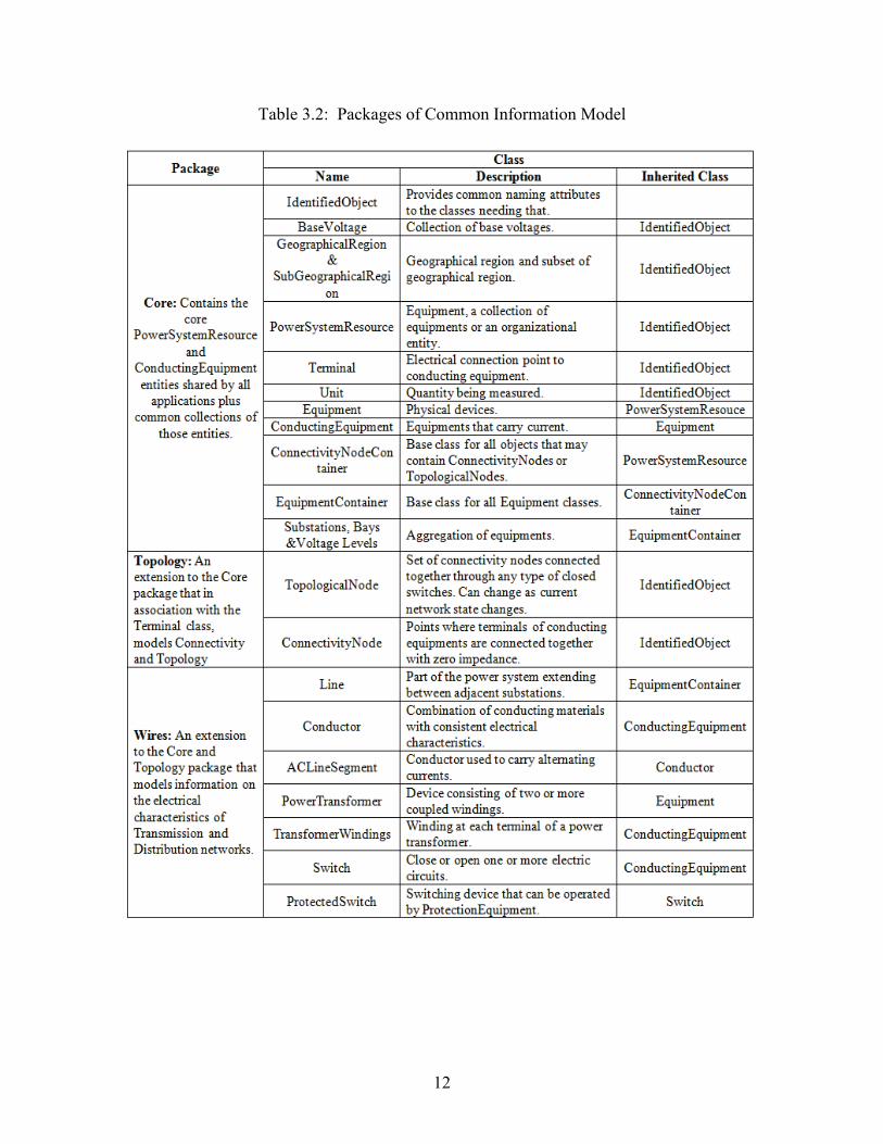
12

Table 3.2: Packages of Common Information Model

13

Table 3.3: Packages of Common Information Model (continued)

(b) Substation Configuration Language (SCL) [23]: SCL (IEC 61850-6) is a standard to describe substation configuration allowing semantic interpretation of substation data. This is also expressed in XML but the data model is not defined using UML. Substation functions are modeled into different logical nodes (LN) which are grouped under different logical devices (LD). Data exchanged between LNs are modeled as data objects, which consist of data attributes. The different components of SCL are described in Table 3.4.

The following files types are the components of SCL:

• System Specification Description (SSD): single line diagram of substation and logical nodes.

• IED Capability Description (ICD): capabilities of an IED.

• Substation Configuration Description (SCD): complete substation configuration.

14

• Configured IED Description (CID): an instantiated IED with all configuration parameters relevant to that IED.

Table 3.4: Contents of Substation Configuration Language

(c) IEEE Standard Common Format for Transient Data Exchange (COMTRADE) [17]: COMTRADE describes syntax of the following files extracted from the raw measurements captured by substation IEDs:

• Configuration files (*.cfg): information for interpreting the allocation of measured data to the equipment (input channels) for a specific substation.

• Data files (*.dat): analog and digital sample values for all input channels (described in configuration file) in substation.

15

4. Unified representation of data and model

4.1 Need for unified representation of data and model

This section addresses the need of unified representation of data and model for improving smart grid applications like fault disturbance monitoring (alarm processing and fault location) and state estimation.

4.1.1 Alarm processing and fault location

Power system components exposed to different weather, as well as human and animal contacts are subject to several types of faults which are caused by random and unpredictable events. Therefore a power system operator should always remain alert by monitoring disturbances caused by faults. Fault disturbance monitoring consists of the following stages:

1. Detection of event: An event is a disturbed power system condition which can be triggered by several causes and can be of different types (fault is one of them).

2. Measurement and Alarm (M&A) processing: A major disturbance can trigger numerous alarms and most of them may be redundant or false. Alarm processors analyze alarm messages and extract information explaining events. It also uses measurements of analog waveforms to draw final conclusions.

3. Fault detection: From the information extracted from the alarm processor, the faulted region is detected by cause-effect analysis of alarms and measurements.

4. Fault location: An exact location of fault is required to help the maintenance crew find and repair the faulted equipment as soon as possible. It is calculated using samples from the transient waveforms.

A fault location monitoring scheme requires adequate information (measurements data as well as power system modeling information) to perform all these four steps successfully.

Figure 4.1 shows the data & information flow in an advanced fault disturbance monitoring implementation. It is evident that all four applications need to communicate with all databases and models and also between them which sometimes results in duplicate information extraction and exchange. As the substations are generally modeled in a detailed node-breaker model while the power system static model is a less detailed bus-branch model, the names and numeric designations of the same power system components described in those two models may become different due to different nomenclature used by various utility groups that maintain given models and data acquisition devices. Nomenclature used in IED database follows that of substation model while nomenclature used in SCADA database follows the similar yet less-detailed static system model expressed in bus-branch. It requires nomenclature correlation tables to correlate between them, which is a very cumbersome process as for each substation separate nomenclature correlation tables are required. Therefore, a significant number of mappings between all types of data and model are required to create a unified correlation between the nomenclatures. Sometimes the mapping has to be done manually or semi-automatically resulting in longer operating time.

16

Figure 4.1: Data and information flow for fault disturbance monitoring

As a result, the following issues are hindering integration and interoperability of data and model for this application:

• Field data collected from various IEDs from different vendors has different data format and information contents.

• Sampling rates and techniques for IED data and SCADA Historian archived data sampling are different.

• The names and numeric designations are different for the same power system components.

Such differences need to be reconciled when interoperability of data and model are sought, and this has to happen at both the semantic and syntactic levels.

Therefore to speed up system restoration under fault disturbances a scheme to represent data and model used in this application in a unified form is required which should have the following features:

• Reduce number of mappings between data and model.

• Correlate different types of data and model without any user intervention.

17

4.1.2 State estimation

We propose a Generalized State Estimation implementation that utilizes dynamic pointer assignment of device terminals. This method allows processing of arbitrary topologies and the estimation function to incorporate switching device status as variables to be estimated. In order to illustrate the method, consider Figure 4.2, which shows the configuration of a very small node-breaker system, comprised of 11 nodes. For simplicity the case includes breakers only, although the method developed supports any type and number of switching devices. The statuses of the breakers at a given point in time results in groups of nodes that correspond to the same electric point (a bus). Figure 4.3 shows the 4-bus bus-branch model, which results from considering the breaker statuses shown in Figure 4.2. The bus-branch case is needed to obtain numerical solutions of the state estimation. The proposed method acts on the unified model and enables representing the system as in Figure 4.2 or as in Figure 4.3 at will, based on the requirements of the applications.

Figure 4.2: 11-node Node-Breaker Model showing bus groupings that will become buses in a

Bus-Branch Model

slack

37 MW9 Mvar

101 MW-28 Mvar

18.68 MW 32 Mvar

A

MVA

A

MVA

A

MVA

7

1

140 MW30 Mvar

120 MW50 Mvar

83 MW41 Mvar

100 MW

4

0 Mvar

10

Figure 4.3: Four-bus planning case corresponding to the 11-node Node-Breaker Model

corresponding to the given breakers statuses.

18

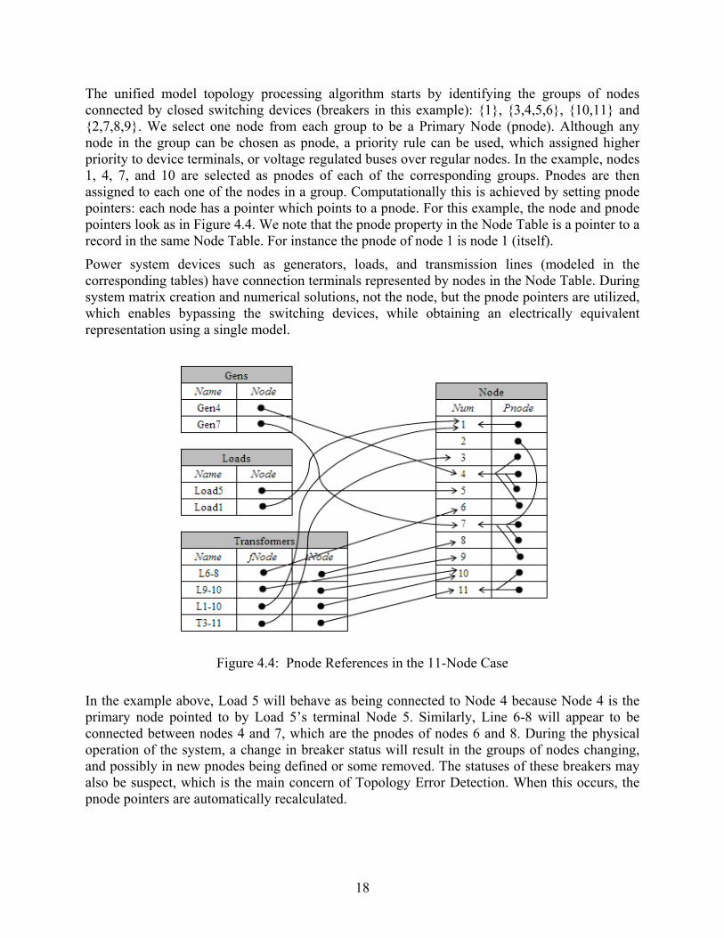
The unified model topology processing algorithm starts by identifying the groups of nodes connected by closed switching devices (breakers in this example): {1}, {3,4,5,6}, {10,11} and {2,7,8,9}. We select one node from each group to be a Primary Node (pnode). Although any node in the group can be chosen as pnode, a priority rule can be used, which assigned higher priority to device terminals, or voltage regulated buses over regular nodes. In the example, nodes 1, 4, 7, and 10 are selected as pnodes of each of the corresponding groups. Pnodes are then assigned to each one of the nodes in a group. Computationally this is achieved by setting pnode pointers: each node has a pointer which points to a pnode. For this example, the node and pnode pointers look as in Figure 4.4. We note that the pnode property in the Node Table is a pointer to a record in the same Node Table. For instance the pnode of node 1 is node 1 (itself).

Power system devices such as generators, loads, and transmission lines (modeled in the corresponding tables) have connection terminals represented by nodes in the Node Table. During system matrix creation and numerical solutions, not the node, but the pnode pointers are utilized, which enables bypassing the switching devices, while obtaining an electrically equivalent representation using a single model.

Figure 4.4: Pnode References in the 11-Node Case

In the example above, Load 5 will behave as being connected to Node 4 because Node 4 is the primary node pointed to by Load 5’s terminal Node 5. Similarly, Line 6-8 will appear to be connected between nodes 4 and 7, which are the pnodes of nodes 6 and 8. During the physical operation of the system, a change in breaker status will result in the groups of nodes changing, and possibly in new pnodes being defined or some removed. The statuses of these breakers may also be suspect, which is the main concern of Topology Error Detection. When this occurs, the pnode pointers are automatically recalculated.

19

We note that there is no need define a Bus class because a Bus Table to store bus objects. Only one class is needed: Node. Because buses are not needed, there is no need to have a bus-branch model. This realizes model unification.

The utilization of pointers to the same type of object (a node) is at the center of the proposed unified algorithm. It is this fundamental principle of using only the Node class that allows unifying the network applications, and which enables supporting flexible generalized functions in the state estimation and topology error detection applications.

4.2 Unified representation of data and model

Unified model representation using same format power system model is discussed in [29]. This unified model allows existing planning software, which inherently uses the bus-branch model, to be used in real-time to solve node-breaker (operations) models. One of the benefits of this unified architecture is that it makes working with bus/branch or node/breaker models transparent to the application. In this manner, unification of planning and operations business processes is achieved at three levels: power system model format, power system model, and power system applications. The unified architecture can be incorporated into generalized state estimation to achieve various benefits:

• Since a single node/breaker is used, no model conversion or device mapping between models needs to take place. Generalized state estimation implemented using a unified architecture will handle a single node array, as opposed to various data structures needed for the objects and mappings required in a two-model framework.

• Processing of suspect regions can be done directly and at will on the node-breaker model. The architecture allows partial pointer relocation of completely arbitrary size and configuration of switching device subnets.

• Architecture can be supported by legacy core state estimator application without requiring fundamental changes to existing numerical code.

Data exchange standards play a major role in automatic exchange of data and information through different applications and within a database. To achieve unified representation of data and models data exchange standards are needed to interpret and exchange data captured in several IEDs and RTUs (from different vendors, having different sampling rates and different naming and nomenclature designations for power system components) and correlating proprietary defined power system models. Although an all-encompassing standard (which may include all the features) is almost impossible to create, we can still unify all related standards (by unifying complementary data models and harmonizing overlapping standard semantics) to expedite automation of fault disturbance monitoring from data and information integration interoperability perspective.

A unified representation of data and model is shown in Figure 4.5. The proposed solution uses standard formats of data and model (CIM for describing power system model and SCADA data; SCL for describing substation model and COMTRADE for describing event data triggered by IEDs) all expressed in node-breaker representation and by using simple rules for representing those data and models interoperability can be achieved.

20

Figure 4.5: Unified representation of data and model

Correlation of COMTRADE files with SCL is easy as they correspond to same substation model. Mapping is required only to correlate between the model and measurements represented in CIM and that of SCL to obtain a uniform representation. Though both CIM and SCL are described in node-breaker model and most of the objects are modeled in a similar way and share same name, some discrepancies are also present.

Several harmonization efforts to properly use CIM and SCL standards can be found in literature [30]-[33]. Formal integration of CIM and SCL by bi-directional mapping between them is addressed in [30]. Mapping for topology processing application is proposed in [31]. Harmonizing these two standards to develop a unified semantic model is discussed in EPRI report [32]. In [33] mismatches between those two standards are addressed and solutions for all types of mismatches are proposed without modifying the original CIM and SCL information model.

The correlation between CIM profile and SCL profiles of different substations is done using the following simple rules:

• For similar objects: Common data structure is used to represent those objects present in both standards.

• For dissimilar objects: Some objects are defined in either of the standards, for those no mapping is needed. Separate data structures for each model are used.

By using the very simple rules mentioned above, data and models used in this fault location application are represented in a unified way. That way automatic correlation can be achieved. Besides, the information extracted from the data and model representation can be used properly in the application.

21

5. Unified representation of data and model for alarm processor and transmission line fault location

5.1 Alarm processor

With the growth of power system complexity, operators are often overloaded with alarm messages generated by the events in the system. A major power system disturbance could trigger hundreds and sometimes thousands of individual alarms and events. Obviously, this is beyond the capacity of any operators to handle. Thus, operators may not able to respond to the unfolding events in a timely manner, and even worse, the event interpretation by the operators may be either wrong or inconclusive affecting their ability to perform expected actions. Operators still have a strong need for a better way to monitor the system than what is provided by the existing alarm processing software [34]. An EPRI study [35] has listed issues that operators face with alarms during the day-by-day operation of a power system:

• Alarms which are not descriptive enough

• Alarms which are too detailed

• Too many alarms during a system disturbance

• False alarms

• Multiplicity of alarms for the same event

• Alarms changing too fast to be read on the display

• Alarms not in priority order

Operators are expected to monitor the system condition and take actions immediately after the alarms occur. However, when all problems mentioned above mix up, operators are severely restrained to perform properly in a timely manner. The task of an intelligent alarm processor is to analyze thousands of alarm messages and extract the information that concisely explains the network events.

A lot of research has been done on the Fuzzy Reasoning Petri-nets (FRPN) [36]-[38]. FRPN takes advantages of Expert System and Fuzzy Logic, as well as parallel information processing to solve the problem of fault section estimation. Reference [39] gives an optimal design of a structure of FRPN diagnosis model.

It has been proven that the logic operand data of digital protective relays can be used as additional inputs to enhance the alarm interpretation [40]. In a digital protective relay, the pickup and operation information of protection elements is usually in the form of logic operands [41]. The pickup and operation logic operands are more reliable than SCADA data because they are more redundant and have less uncertainty than relay trip signals and circuit breaker status signals.

In such a solution, input data such as relay trip signals and circuit breaker status signals are acquired by RTUs of the SCADA system. Relay logic operand signals are defined in their data memories and retrieved from relays by the SCADA front-end computers in substations. The data are acquired from different substations and are transmitted to the control center through selected

22

communication link such as microwave or optical fiber. In the control center, the SCADA master computer puts the input data into a real-time data base and keeps updating them at each scan time.

In the previous ERCOT project report [42], the data requirement has been presented, as shown in the Table 5.1.

Table 5.1: Data and related sources required for Intelligent Alarm Processor

Type of Data Related Source Description One-line display

System Configurations This file contains the information about the system connectivity.

Alarm Log data

Data from RTU of SCADA 1. CB status change alarms (Opening and

Closing) 2. Report-by-exception alarms (Over-current,

under-voltage, and other values exceeding some threshold, etc.)

This file contains the alarm messages appeared in the control center when fault actually occurred.

Data from DPR (additional data) 1. Pickup & Operation signals of Main

Transmission Line Relays 2. Pickup & Operation signals of Primary

Backup Transmission Line Relays 3. Pickup & Operation signals of Secondary

Backup Transmission Line Relays 4. Pickup & Operation signals of Bus Relays

5.2 Transmission line fault location

Transmission lines are generally exposed to several types of faults which are usually caused by random and unpredictable events such as lightning, short circuits, overloading, equipment failure, aging, animal/tree contact with the line, human intended or unintended actions, lack of maintenance etc. Protective relays, placed at both ends of a transmission line sense the fault immediately and isolate the faulted line by opening the associated circuit breakers. Faults may be temporary (fault is cleared after breaker re-closing) or permanent (fault is not cleared even after several re-closing attempts). To restore service after permanent fault, an accurate location of the fault is highly desirable to help the maintenance crew find and repair the faulted line section as soon as possible.

Though distance relays are the fast and reliable ways to locate the faulted area, they cannot meet the need of accurate fault location under all circumstances. They may over-reach or under-reach due to several unknown parameters, such as pre-fault loading, fault resistance, remote infeed, etc.

Transmission line faults may be calculated either using power frequency components of voltage and current or higher frequency transients generated by the fault [43]-[44]. Phasor based methods use fundamental frequency component of the signal and lumped parameter model of the line

23

while time-domain based methods use transient components of the signal and distributed parameter model of the line. Both of these methods can be subdivided into two more broad classes within each category depending upon the availability of recorded data: single-end methods [45]-[47] where data from only one terminal of the transmission line is available and double-end methods [48]-[52] where data from both (or multiple) ends of the transmission line can be used. Double-ended methods can use synchronized or unsynchronized phasor measurements, as well as synchronized or unsynchronized samples.

Travelling wave-based fault location approaches [53]-[55] use transient signals generated by the fault. They are based on the correlation between the forward and backward travelling waves along a line or direct detection of the arrival time of the waves at terminals.

Each of the techniques requires very specific measurements from one or both (multiple) ends of the line to produce results with desired accuracy. However, availability of data in particular location may be a challenging issue.

Installing recording devices (DFRs in our case) at the ends of all the transmission lines may not be feasible, as the case is with tapped lines. Although protective relays exist on every transmission line and isolate the faulted line by opening the associated circuit breaker when sensing fault immediately, most of them may still be electromechanical and they do not have capability to record measurements. As a result, in some cases, it may happen that there are no recordings at all available at line ends close to a fault. System-wide sparse measurement based fault location method can be applied in such instances [56]-[57].

In sparse measurement based fault location method, phasor measurements from different substations located in the region where the fault has occurred are used. The measurements are considered sparse, as they may come from only some of many transmission line ends (substations) in the region. This method requires synchronization of the samples and extracted features (measurements), which may be obtained by using DFRs connected to Global Positioning System (GPS) receivers. Besides the sparse measurements, the technique also uses a commercial short circuit program tool PSS/E, which is initialized with power system model (expressed as bus branch model) and tuned with SCADA Historian data scan, which is a set of RTU measurements associated with the time of the fault occurrence. The method uses waveform matching technique between the current and voltage phasors calculated from the samples of waveforms recorded in a substation (nearby the faulted line) and phasors simulated using short circuit calculation of possible fault locations. The calculated and simulated phasors are compared while the location of the fault is changed in the short circuit program. This process of placing faults in different locations is repeated automatically until the difference between measured and simulated phasor values reaches global optimum (minimum), which indicates that the fault location used in the short circuit program is the actual one in the field. The criteria for the minimal difference are based on a global optimization technique that uses Genetic Algorithm.

Again, to speed up system restoration under fault disturbances, fault location requires handling and exchanging data and information automatically as well as performing the fault location automatically. A unified representation of data and models is required to achieve interoperability between data and model as well as fault location application so that a seamless data and information transfer is possible automatically.

Considering all these factors stated above, an optimal fault location scheme to locate transmission line faults should have the following characteristics:

24

• Properly use all available data

• Unify data and model automatically

• Smartly choose appropriate algorithm depending on the availability of data

An optimal fault location scheme proposed in [58] is implemented using unified representation of data and model. The flowchart of the scheme is shown in Figure 5.1 .

Figure 5.1: Optimal fault location

The measured data and models associated with optimal fault location application are:

• Event data: These include event data captured by recording devices (DFRs here) after occurrence of a fault.

• SCADA Historian data: This data reflects real time changes in the power system including the latest load, branch and generator data to tune the static system model with the actual pre and post fault conditions.

25

• Power system static model data: These include power flow system specification data for the establishment of a static system model (in PSS/E *.raw format).

5.3 Unified representation of data and model for intelligent alarm processor and optimal fault locator

5.3.1 Data and model for a test case

The unified representation of data and model is implemented on a small power system model for simplicity of description. As there are no standard test cases available for both CIM model and SCL model, we have used the following model data and took some assumptions to artificially generate a fault case:

• A small power system network (expressed in CIM model) is chosen, which is obtained from a sample system used in [59]. The detailed node-breaker representation of the power system network is shown in Figure 5.2.

Figure 5.2: Node-breaker representation of small power network [59]

• Several faults on the line between Bus-2 and Bus-5 are considered. We are assuming that DFR installed on Bus-4 is triggered due to the fault. Figure 5.3 shows the bus-branch representation of the faulted power system network. The fault is simulated in ATP [60] and the pre-fault, during-fault and post-fault voltage and current signals at Bus-4 are recorded and converted to COMTRADE format using the Output Processor [61].

26

Figure 5.3: Bus-branch representation of small power network

• As no corresponding SCL models are available for the substation 1 (Bus-4), example from IEC 61850-6 standard is used. The detailed node-breaker diagram for the substation is shown in Figure 5.4.

Figure 5.4: Node breaker representation of Substation-1

27

• The following changes are made in the above models for uniformity:

a. As the voltage levels in CIM model and SCL models were different we have changed the voltage level in SCL model to that of CIM.

b. In SCL a switch and breaker combination (QB1 & QA1) is present between Busbar (W1) and transformer (T1) while in CIM only a switch (S16) is present between Bus1 and TR1. For uniformity we have added a breaker (B8) between S16 and TR1 in substation -1 in CIM xml file.

5.3.2 Implementation procedure

The detailed implementation procedure is discussed in brief:

5.3.2.1 Power system static model

A CIM profile of power system objects needed to model static power system is chosen. All the equipments (generator, load, line, transformer, breaker, disconnector etc.) have one or two terminals. Connectivity nodes are points where terminals of conducting equipments are connected together with zero impedance. In CIM connectivity and topology of power network can be determined by terminals and connectivity nodes and switch status. Topology of the system changes with change of switching status of breakers and diconnectors.

Power system static model in base case for the small network expressed in CIM XML file [59] is processed in the following steps:

• The XML file is parsed and all the objects with same nomenclature with the XML file are assigned with the values obtained from the XML file.

• Topological node for base case determination: Topological Node is a set of connectivity nodes that, in the current network state, are connected together through any type of closed switches, including jumpers. Topological nodes can change as the current network state changes (i.e., switches, breakers, etc. change state). A topological node corresponds to bus in equivalent bus-branch model. All topological nodes for the base case are determined using the algorithm presented in [62]. The algorithm starts from primary equipment (i.e. generator, transformer, load, line) and scans through all closed switches and groups the connectivity nodes associated in a single topological node and stops when another primary equipment is found. The node-breaker representation of the static power system model is shown in Figure 5.5 (all of the switches are closed). Small black dots represent terminals and large black dots represent connectivity nodes. Bus-branch model of the same network by creating topological nodes (in box with dash lines) is shown in Figure 5.6.

• Selection of pNode: A primary node (pNode) is selected [29]. In the topological node determination algorithm, the 1st connectivity node in a topological node is usually a primary equipment; therefore the 1st connectivity node in a topological node is selected as pNode. The other connectivity nodes in that topological node point that pNode which corresponds to bus in equivalent bus-branch model. The pNodes in all the topological nodes are shown in Figure 5.6.

28

• Extraction of PSS/E data: As our fault location method uses short circuit program in PSS/E, the PSS/E raw data (expressed in bus branch representation) is extracted [62]-[63] where the bus names are actually the connectivity node names and therefore no nomenclature correlation between node-breaker model and bus-branch model is required.

Figure 5.5: Node-breaker representation with terminals and connectivity nodes

Figure 5.6: Bus-branch representation with topological nodes

29

5.3.2.2 Tuning static system model

Power system static model should be updated with the pre-fault conditions (switching changes and load/generation changes). CIM dynamic file [64] consists of measurement data with time stamps. As we don’t have this, a model of the small power system in ATP is used to generate measurements. Breaker and disconnector status updates are used to perform incremental topology processing [29] where topological nodes are recreated with changed switch status.

5.3.2.3 Detailed substation model in SCL

In SCL substation functions are modeled into different logical nodes (LN) which are grouped under different logical devices (LD). All the logical nodes are associated to IEDs. Data exchanged between LNs are modeled as data objects, which consist of data attributes. SCL file for a selected substation is processed using the following steps:

• The XML file is parsed and all the objects with same nomenclature with the XML file are assigned with the values obtained from the XML file.

• For objects present in CIM (i.e. power transformer, voltage level etc.) both CIM and SCL names are stored so that no naming correlation required later. (discussed in next section).

• The IED names correspond to the logical nodes for measurement purpose are stored which helps finding the COMTRADE file for the recorder.

5.3.2.4 Event data in COMTRADE

The raw measurement captured in DFR present in the substation are processed with the knowledge obtained from the configuration file (*.cfg) of the data (*.dat) in COMTRADE.

5.3.2.5 Unified representation

The unified representation of data and model is achieved using the following rules:

• Common data structures are used for similar objects. For example both of the models have substation object in common. Figure 5.7 shows the CIM representation and Figure 5.8 shows the SCL representation.

Figure 5.7: Substation object in CIM

30

Figure 5.8: Substation object in SCL

A class substation defined in our program has the following description:

Substation.name.cim="Substation1"

Substation.name.scl="S12"

Substation.VoltageLevel.high.name.cim="Substation-1 220KV"

Substation.VoltageLevel.low.name.cim="Substation-1 15KV"

Substation.VoltageLevel.high.name.scl="E1"

Substation.VoltageLevel.low.name.scl="D1"

The other objects inside Substation object are defined in same fashion.

• Separate data structures for each model for dissimilar objects. For example CIM has ThermalGeneratingUnit but SCL doesn't. Figure 5.9 shows the CIM representation.

Figure 5.9: ThermalGeneratingUnit object in CIM

A class ThermalGeneratingUnit within substation is defined in our program has the following description:

Substation.ThermalGeneratingUnit.name="GEN1"

• In some cases both similar and dissimilar objects are present which represent same electrical equipment. Both common and separate data structures within the object are used. For example both CIM and SCL have PowerTransfrmer object while SCL also include IED associated to that (TCTR i.e. current transformer LN here). Figure 5.10 shows the CIM representation and Figure 5.11 shows the SCL representation of PowerTransformer.

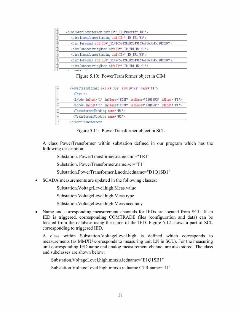
31

Figure 5.10: PowerTransformer object in CIM

Figure 5.11: PowerTransformer object in SCL

A class PowerTransformer within substation defined in our program which has the following description:

Substation. PowerTransformer.name.cim="TR1"

Substation. PowerTransformer.name.scl="T1"

Substation.PowerTransformer.Lnode.iedname="D1Q1SB1"

• SCADA measurements are updated in the following classes:

Substation.VoltageLevel.high.Meas.value

Substation.VoltageLevel.high.Meas.type

Substation.VoltageLevel.high.Meas.accuracy

• Name and corresponding measurement channels for IEDs are located from SCL. If an IED is triggered, corresponding COMTRADE files (configuration and data) can be located from the database using the name of the IED. Figure 5.12 shows a part of SCL corresponding to triggered IED.

A class within Substation.VoltageLevel.high is defined which corresponds to measurements (as MMXU corresponds to measuring unit LN in SCL). For the measuring unit corresponding IED name and analog measurement channel are also stored. The class and subclasses are shown below:

Substation.VoltageLevel.high.mmxu.iedname="E1Q1SB1"

Substation.VoltageLevel.high.mmxu.iedname.CTR.name="I1"

32

Figure 5.12: Part of SCL corresponding to triggered IED

By using the rules mentioned above, correlation between data and models are achieved automatically. After correlation of data and model, required information (voltage and current phasors for pre-fault and faulted network for each of the monitored channel mentioned in COMTRADE configuration file, status of the breakers from COMTRADE data file, relay trip signals from COMTRADE data file, SCADA measurements) are extracted as in [57].

5.3.3 Case study results

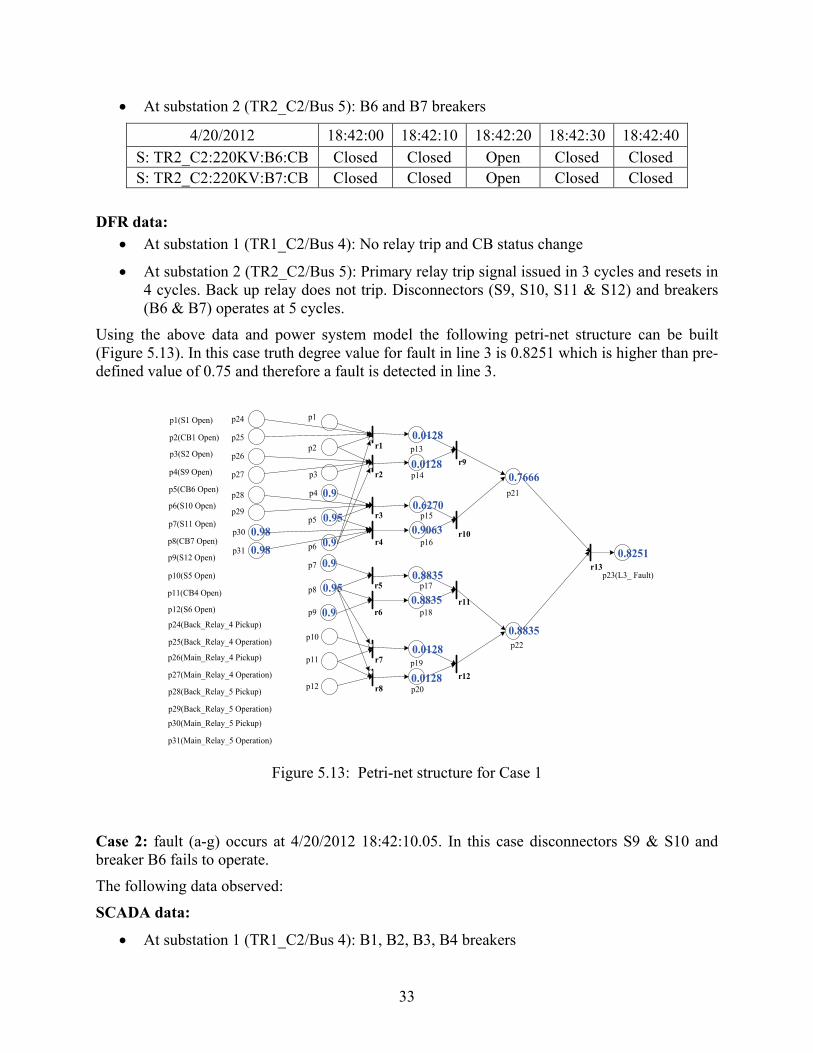
A fault (ag) occurs at 4/20/2012 18:42:10.05 on line 3 (midway of the 60 mile line).

5.3.3.1 Alarm processor

Two test cases are performed.

Case 1: fault (ag) occurs at 4/20/2012 18:42:10.05.

Fault interrupted in 1 sec after and all the switches closed and re-energized the circuit 1 sec after the fault interruption.

The following data observed:

SCADA data:

• At substation 1 (TR1_C2/Bus 4): B1, B2, B3, B4 breakers

4/20/2012 18:42:00 18:42:10 18:42:20 18:42:30 18:42:40 S: TR1_C2:220KV:B1:CB Closed Closed Closed Closed Closed S: TR1_C2:220KV:B2:CB Closed Closed Closed Closed Closed S: TR1_C2:220KV:B4:CB Closed Closed Closed Closed Closed S: TR1_C2:220KV:B5:CB Closed Closed Closed Closed Closed

33

• At substation 2 (TR2_C2/Bus 5): B6 and B7 breakers

4/20/2012 18:42:00 18:42:10 18:42:20 18:42:30 18:42:40 S: TR2_C2:220KV:B6:CB Closed Closed Open Closed Closed S: TR2_C2:220KV:B7:CB Closed Closed Open Closed Closed

DFR data: • At substation 1 (TR1_C2/Bus 4): No relay trip and CB status change

• At substation 2 (TR2_C2/Bus 5): Primary relay trip signal issued in 3 cycles and resets in 4 cycles. Back up relay does not trip. Disconnectors (S9, S10, S11 & S12) and breakers (B6 & B7) operates at 5 cycles.

Using the above data and power system model the following petri-net structure can be built (Figure 5.13). In this case truth degree value for fault in line 3 is 0.8251 which is higher than pre-defined value of 0.75 and therefore a fault is detected in line 3.

p1(S1 Open)

p2(CB1 Open)

p3(S2 Open)r1

p23(L3_ Fault)

r2

r3

r4

p13

p14r9

r13

0.9

0.95

0.9

0.0128

0.01280.7666

0.8251

r7

r8

p19

p20r12

0.0128

0.0128

p15

p16

0.6270

0.9063

r5

r6

0.9

0.95

0.9

p17

p18

0.8835

0.8835

r10

r11

0.8835

0.980.98

p11

p12

p10

p9

p8

p7

p6

p5

p4

p3

p2

p1

p21

p22

p24

p25

p26

p27

p28

p29

p30

p31

p4(S9 Open)

p5(CB6 Open)

p6(S10 Open)

p7(S11 Open)

p8(CB7 Open)

p9(S12 Open)

p10(S5 Open)

p11(CB4 Open)

p12(S6 Open)

p24(Back_Relay_4 Pickup)

p25(Back_Relay_4 Operation)

p26(Main_Relay_4 Pickup)

p27(Main_Relay_4 Operation)

p28(Back_Relay_5 Pickup)

p29(Back_Relay_5 Operation)

p30(Main_Relay_5 Pickup)

p31(Main_Relay_5 Operation)

Figure 5.13: Petri-net structure for Case 1

Case 2: fault (a-g) occurs at 4/20/2012 18:42:10.05. In this case disconnectors S9 & S10 and breaker B6 fails to operate.

The following data observed:

SCADA data:

• At substation 1 (TR1_C2/Bus 4): B1, B2, B3, B4 breakers

34

4/20/2012 18:42:00 18:42:10 18:42:20 18:42:30 18:42:40 S: TR1_C2:220KV:B1:CB Closed Closed Closed Closed Closed S: TR1_C2:220KV:B2:CB Closed Closed Closed Closed Closed S: TR1_C2:220KV:B4:CB Closed Closed Closed Closed Closed S: TR1_C2:220KV:B5:CB Closed Closed Closed Closed Closed

• At substation 2 (TR2_C2/Bus 5): B6 and B7 breakers

4/20/2012 18:42:00 18:42:10 18:42:20 18:42:30 18:42:40 S: TR2_C2:220KV:B6:CB Closed Closed Closed Closed Closed S: TR2_C2:220KV:B7:CB Closed Closed Open Closed Closed

DFR data:

• At substation 1 (TR1_C2/Bus 4): No relay trip and CB status change

• At substation 2 (TR2_C2/Bus 5): Primary relay trip signal issued in 3 cycles and resets in 4 cycles. Back up relay does not trip. Disconnectors (S11 & S12) and breakers (B7) operates at 5 cycles.

Using the above data and power system model, the following petri-net structure can be built (Figure 5.14). In this case, truth degree value for fault in line 3 is 0.5693, which is lower than pre-defined value of 0.75 due to very few alarm inputs and failure of devices.

p1(S1 Open)

p2(CB1 Open)

p3(S2 Open)r1

p23(L3_ Fault)

r2

r3

r4

p13

p14r9

r13

0.2550

0.25500.2550

0.5693

r7

r8

p19

p20r12

0.0128

0.0128

p15

p16

0

0.2763

r5

r6

0.9

0.95

0.9

p17

p18

0.8835

0.8835

r10

r11

0.8835

0.980.98

p11

p12

p10

p9

p8

p7

p6

p5

p4

p3

p2

p1

p21

p22

p24

p25

p26

p27

p28

p29

p30

p31

p4(S9 Open)

p5(CB6 Open)

p6(S10 Open)

p7(S11 Open)

p8(CB7 Open)

p9(S12 Open)

p10(S5 Open)

p11(CB4 Open)

p12(S6 Open)

p24(Back_Relay_4 Pickup)

p25(Back_Relay_4 Operation)

p26(Main_Relay_4 Pickup)

p27(Main_Relay_4 Operation)

p28(Back_Relay_5 Pickup)

p29(Back_Relay_5 Operation)

p30(Main_Relay_5 Pickup)

p31(Main_Relay_5 Operation)

Figure 5.14: Petri-net structure for Case 2

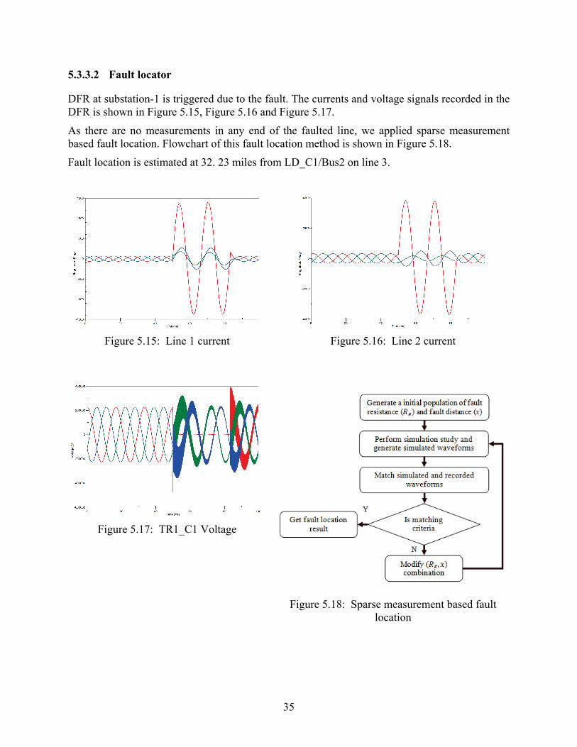
35

5.3.3.2 Fault locator

DFR at substation-1 is triggered due to the fault. The currents and voltage signals recorded in the DFR is shown in Figure 5.15, Figure 5.16 and Figure 5.17.

As there are no measurements in any end of the faulted line, we applied sparse measurement based fault location. Flowchart of this fault location method is shown in Figure 5.18.

Fault location is estimated at 32. 23 miles from LD_C1/Bus2 on line 3.

Figure 5.15: Line 1 current

Figure 5.16: Line 2 current

Figure 5.17: TR1_C1 Voltage

Figure 5.18: Sparse measurement based fault

location

36

6. Unified generalized state estimator

6.1 Introduction

State Estimator is an essential tool for real-time power system monitoring, and a prerequisite for real-time security analysis, control, and economic applications. The utilization of state estimators is becoming more important at all levels of transmission and distribution systems as an enabling technology for electricity control, automation, and smart grid applications. Because the success of control objectives depends heavily on the ability to accurately determining the state of controlled devices and subsystems, having flexible state estimation functions at all levels of the electricity system is of paramount importance to realizing future electricity systems.

The conventional state estimator used today at both the transmission and distribution levels, has limitations regarding the assumption of statuses of switching devices. An undetected topology error can completely undermine the estimator performance. Generalize State Estimators (GSE) [12] incorporate breaker status as variables to be estimated. A significant aspect of the GSE application is related to the need to address two types of representations: node-breaker and bus-branch. GSEs have not been widely accepted in the industry because its implementation is cumbersome due to the following:

• Breaker status information is only available at the physical, node-breaker model prior to topology processing. In order to identify and resolve topology errors, the GSE must handle and maintain mappings between the two node-breaker and bus/branch structures, which usually requires auxiliary mapping routines.

• During the solution, GSE must alter the bus/branch topology as suspect breaker statuses are processed. Thus all the mappings must be dynamically updated, which is computationally inefficient.

• State estimators algorithms use a bus/branch model to perform the numerical computations, at it is not trivial to incorporate generalized states in existing code data structures. In particular, the positions of state variables associated with SE matrices needs to be dynamically updated as subnets are collapsed and expanded realizing newly formed or split buses.

Production environment installed state estimators are not of generalized type. The existing state estimator uses breaker level models on an “as needed” basis and does it based on the dc model only. Detailed modeling of substations has been suggested several decades ago by Irving and Sterling, who also laid out the formulation of a substation state estimation. These ideas were later expanded by the introduction of zero impedance branch models to represent breakers by Monticelli [65]. His approach has been used by many other researchers to develop detailed models to identify breaker status errors. These include not only positive sequence, but also three phase models as well. All of the approaches, however, assume that only a very small part of the system will be modeled in detail and state estimation function will still carry out a bus level solution for major part of the system.

The unified architecture described in previous sections can be used to transparently handling arbitrary switching device topologies. Since the core routine of the GSE consists in reducing and expanding portions of the network with suspect breaker statuses, handling switching topologies

37

at will is critical for computational speed. In this section, we combine the model unification ideas with topology error detection under generation state estimation framework.

6.2 Topology error detection framework

The Topology Processing (TP) function assumes a given status of circuit breakers and converts the node/breaker model into a bus/branch representation where estimation takes place. This process is inherently limited, because topology errors at the node/breaker level may result in an incorrect bus/branch description of the system and possible divergent or erroneous state estimation results. Detecting topology errors at the node/breaker level is thus necessary to enhance, often to make possible the overall estimation process. The analysis of topology errors prior to topology processing is called Topology Error Detection (TED). A two-phase process can be utilized to identify and remove topology errors. The first phase consists of a local minimization of the flow estimate errors performed separately for each subnet. If all subnet measurements and all circuit breaker statuses are correct, estimation results in very small residuals, which would indicate absence of erroneous indications. Subnets with small flow residuals can be consolidated by Topology Processing without risk. Suspect subnets remain modeled at the node-breaker level. In phase two, a system-wide generalized state estimation takes place to determine potentially interacting topology errors. Once the remaining topology errors are determined, Topology Processing processes the remaining subnets. If no suspect subnets are present after phase one, phase two does not take place. Both phases of the topology error detection take place using active power flows as state variables.

6.3 Local (subnet) topology error detection

6.3.1 Generalized flows

A subnet is defined as a set of switching devices and bus sections that have the same nominal voltage level. A substation usually has at least one subnet per voltage level. The boundaries of the subnet are given by the terminals of the power system physical devices, for instance a generator, a switched shunt, a load, a terminal of a transmission line or a leg of a transformer. Figure 6.1 shows the configuration of a simple subnet. Subnets are determined at the beginning of Topology Error Detection.

LOADGEN

LINE A LINE B

1

2

3

5

4 6

Figure 6.1: Simple Subnet Configuration

38

The subnet shown in Figure 6.1 has six nodes, which have been numbered from 1 to 6, and seven breakers. The end of transmission lines A and B, together with the generator and the load, represent injections to the subnet. The sample subnet has injections at nodes 1, 4, 5 and 6. We can assign an arbitrary direction to the seven flows of active power through circuit breakers. In a generalized sense, we can also consider the four injections as branch flows, too. In the subnet in this example, the active power flows can be modeled using 11 flow variables as shown in Figure 6.2.

Figure 6.2: Subnet Flow Variables

The utilization of flow variables has the following advantages:

• It does not involve the use of Ohm’s Law, since this would become inapplicable in the presence of breakers. Breakers represent zero impedance branches.

• It allows determining estimates for the active power flows, including flows through breakers the breakers.

• It unifies the treatment of variables avoiding the use of the voltage magnitudes or angle as state variables.

Using the definition of the flow variables, one can write the following node balance equation at each one of the 6 nodes:

1 8

1 2 4 5 7

3 6 7

2 3 10

4 9

5 6 11

1: 02 : 03: 04 : 05 : 06 : 0

n f fn f f f f fn f f fn f f fn f fn f f f

= + =

= − + + + + == − − − == − + + == − + == − + + =

6.1

39

Let us assume that the system has megawatt measurements at the generator, the load and Line B, as follows:

1

5

4

10 MW15 MW

8 MW

fff

= −== −

6.2

These would represent measurement equations for the system. In addition, we can write breaker status equations for the breakers that are open:

3

6

00

ff==

6.3

Finally, we can state the subnet power balance equation which says that the sum of all injections to the subnet must be zero:

8 9 10 11 0f f f f+ + + = 6.4

We consider the balance equations of each node, the zero flow through open circuit breakers, and the subnet flow balance as pseudo-measurements. Thus, we can set up a system of equations with measurements and pseudo-measurements as the right-hand vector.

Table 6.1: System of Equations for Subnet Flows

1 2 3 4 5 6 7 8 9 10 11

Breakers Injections

1 1 01 1 1 1 1 0

Nodes 1 1 1 01 1 1 0

1 1 01 1 1 0

1 10Measurements 1 15

1 8Breaker 1 0Statuses 1 0Subnet Ba

f f f f f f f f f f f z

−− − −

−−

−−

−

1 1 1 1 0lance

40

We note that the upper-left submatrix of the breaker and node coefficients is precisely the subnet branch-to-node incidence matrix, which is easily formed. The left upper matrix corresponds to the injections to the subnet nodes. Forming the rest of the matrix is trivial.

Let us denote the vector of active power flows as f, the matrix just formed as H, and the right-most column of measurements and pseudo-measurements as z. Thus, considering the size of these matrices and vectors, the system of equations can be written in matrix form as:

(12 11) (11 1) (12 1)x x x

=H f z 6.5

We want to find the vector f, given H and z. Clearly this is a linear over-determined case, and therefore we can use estimation. Considering the same weights for the pseudo-measurement vector z, the state of the subnet given by the active power flows is obtained as:

1T T− = f H H H z 6.6

The estimated pseudo-measurements are thus determined as:

ˆ =z Hf 6.7

6.3.2 Local error detection

To demonstrate the problem of erroneous status, let us consider the following cases:

Case A: The system described by Equations 6.1-6.4, which results in the system of equations shown in Table 6.1. If Equations 6.6 and 6.7 are applied for this case, the flow vector f is consistent with all the equations, and the estimated and measured values of z are the same: ˆ =z z . The pseudo-measurement residuals are hence zero. These values of Case A are listed in Table 6.2 and Table 6.3, under the corresponding columns.

Case B: Suppose now that besides the load, generator and Line B measurements in Equation 6.2 we have a measurement of Line A, f10 = −16. The sum of injections to the subnet is different from zero, and this is reflected on the flows and estimates as shown in the Case B columns of Table 6.2 and Table 6.3. We note that the residuals are different from zero, but are small. We can conclude that there is some error in the subnet measurements, but that the set is consistent and this error is allowable. The subnet can be processes.

Case C: Starting with Case B (additional measurement in Line A), suppose that the indication of the breaker status corresponding to flow f2 is incorrect and is reported as open. Then, a new pseudo-measurements must be added together with the equation f2 = 0 and the corresponding row in the matrix H. The estimated flows now differ considerably from the condition reported for Case B. The largest residual of the estimated pseudo-measurements, −4.652 corresponds to equations of flows f2 = 0 and f3 = 0. Thus either circuit breaker f2 or f3 is actually closed and both pseudo-measurements are considered suspect. If f3 is closed, then the flow could reach node 2 through f7, ending up with consistent flows. If either one of these pseudo-measurement is removed from the set, the estimation process will produce the results shown for Case B. Note that the sum of squared residuals J increased significantly compared with the value of J in Case B, clearly pointing out the existence of bad pseudo-measurements/indications.

41

Case D: Finally, starting with Case B, consider breaker f4 wrongly reported as open. A pseudo-measurement f4 = 0 must be added. Note that there was already a non-zero measurement f4, which must be preserved in the set to counteract a potentially wrong indication. The results of the estimation process are listed under Case D column on Table 6.2 and Table 6.3. Table 6.3 shows that the largest residual occurs for the pseudo-measurement f4 = 0, which points out the presence of wrong indications. When this pseudo-measurement is removed from the set, the results return to be those of Case B.

Table 6.2: Estimated Flows (MW)

CASE A B C D f1 -10.000 -9.851 -8.762 -9.195 f2 -17.000 -16.234 -4.652 -17.264 f3 0.000 0.000 4.652 0.000 f4 -8.000 -8.149 -9.238 -4.402 f5 15.000 14.851 13.762 14.195 f6 0.000 0.149 1.238 0.805 f7 0.000 -0.234 -7.262 -1.264 f8 10.000 9.787 8.896 8.851 f9 -8.000 -8.213 -9.104 -4.747 f10 -17.000 -16.149 -12.585 -16.805 f11 15.000 14.638 12.659 13.046

Table 6.3: Pseudo-Measurement Residuals

CASE A B C D n1 0.000 0.064 -0.134 0.345 n2 0.000 -0.085 -1.372 -0.460 n3 0.000 -0.085 -1.372 -0.460 n4 0.000 -0.085 3.281 -0.460 n5 0.000 0.064 -0.134 0.345 n6 0.000 0.064 -0.134 0.345 f1 0.000 -0.149 -1.238 -0.805 f5 0.000 0.149 1.238 0.805 f4 0.000 0.149 1.238 -3.598 f10 0.149 -3.415 0.805 f3 0.000 0.000 4.652 0.000 f6 0.000 -0.149 -1.238 -0.805 f2 -4.652

f4 STATUS 4.402 Balance 0.000 -0.064 0.134 -0.345

J 0.000 0.149 75.676 36.023

Weights can be utilized as part of the error detection as in standard WLS estimation. In particular, pseudo-measurements of zero node balance and subnet balance could have larger

42

weights. However, it is advisable to not set the weights too high because some error in injection measurements of transmission lines is expected in realistic cases.

In most real systems, most subnets have around 10 to 20 breakers. However there are subnets with up to 70 and 80 breakers. Including injections, a subnet will very rarely have more than 100 states. However, this number may be tripled if disconnects are modeled. Thus, sparse matrix techniques may be used with marginal advantage.

6.3.3 Subnet observability

In our previous example, imagine that a case where the load measurement f4 is lost. The last row of the measurements sub-matrix is removed. One may think the system to be solvable since we still have a (11 x 11) H matrix. However, the resulting matrix is linearly dependent and hence singular. The subnet is thus not observable. There are infinite solutions, which can be confirmed by noting that for any value of the Line A flow, there will be a calculated value for the load. The same effect will be seen if for instance breaker with flow f6 would actually be closed and hence the zero pseudo-measurement would be removed. In this case it is not possible to determine which part of the flow from f11 goes through f5 and which portion goes through f6 → f7. These flows would be not observable.

If the subnet is not observable, topology errors cannot be detected based on subnet information only. More information is needed. An alternative is to consolidate the subnet if the injection balance equation is zero or if the subnet electric areas injection balance equations are zero.

Observability of the subnet is loosely related to that of the entire system. Assuming there are no errors in topology, the sample subnet would be consolidated by Topology Processing into a single bus, with measurements at the generator and at line B. Observability will be achieved if a flow in line A can be determined, which can be determined from measurements at the other end of the lines and from measurements in connecting subnets. Assuming the subnet is left at the node/breaker model if it is found to not be observable, the subnet topology error detection phase takes place individually for each subnet as shown in Figure 6.3.

43

Figure 6.3: Subnet Topology Error detection

6.3.4 Local TED processing logic

Table 6.4 shows the Subnet Records for a case with 10,000 nodes. Fields include primary nodes, the list of nodes, and the number of breakers, measurements, etc. The TED outcome (either TED_Pass or TED_Fail) is also shown. The subnets have been sorted in descending order by the value of the largest pseudo-measurement residual. Two subnets present residuals larger than 0.05 and are considered to have an erroneous indication/measurement.

TED starts by determining the system subnets and the primary node, and by creating a list of the corresponding nodes, breakers, measurements, indications and injections. Then pseudo-measurements are added and the pseudo-measurement Jacobian H is formed as in Table 6.2. The table shows the subnet topology status, which may be:

Not_Processed: If the subnet has not been processed yet either by Topology Error Detection or by Topology Processing.

TED_Failed: If the subnet was not observable, or became not observable due to bad pseudo-measurement removal.

TED_Passed: If the subnet was observable and the pseudo-measurement residuals were all below a certain threshold. For active power, the default threshold is of 0.05 puMW. Consolidated: If the electric areas inside the subnet have been consolidated

CB Status Changed: If there has been a change in status of a subnet breakers and its topology must be reevaluated.

44

Table 6.4: Subnet TED Output

Subnet Nodes CBs Injections Meas. Largest Residual

Status

1 20 20 7 47 0.5485 TED Failed 2 18 20 8 48 0.5232 TED Failed 3 5 4 3 11 0.0497 TED Passed 4 11 10 10 30 0.0494 TED Passed 5 4 3 3 9 0.0490 TED Passed 6 11 11 7 29 0.0388 TED Passed 7 4 3 3 9 0.0342 TED Passed 8 3 2 2 6 0.0335 TED Passed 9 11 10 10 30 0.0312 TED Passed 10 8 8 4 20 0.0305 TED Passed

Within a Subnet, most residuals will be small, within the 0.05 puMW threshold. Pseudo-measurements that exceed the threshold are removed and tagged. A measurement or pseudo-measurement can have the following TED flags:

TED_Good: If the pseudo-measurement has a residual below the threshold.

TED_Removed: If the pseudo-measurement was removed from the set

TED_Fixed: If the pseudo-measurement was corrected to its estimated value

6.4 Generalized state estimation

Subnets detected as not observable due to not having enough measurements (or the measurement set progressively being reduced due to large residuals) are preserved in the case modeled at the node/breaker level. Subnets that reported no errors on measurements or indications, or those whose errors were detected and fixed are processed by topology processing. In most systems, none or just a few subnets will remain not consolidated after the local TED.

The second phase of topology error detection consists of performing a generalized estimation for the entire system, using breaker active power flows as state variables in addition to all regular state estimation variables and states. This has the advantage of obtaining flows through remaining circuit breakers as a by-product of the analysis, but the implementation is more difficult, because a new type of state (breaker flow) must be introduced, and because those states may be dynamically added during the state estimation solution.

In order to form the H matrix, in the same manner as with local TED, injections to the system are identified and set up in the equations. However, no system injection balance equation can be assumed due to system losses. Injections will be of generator or load type, but not of transmission line type. If a transmission line has different flow measurements at both ends of the line, both measurements are included in the measurement sub-matrix. Line flows are directed and those measurements will have opposite direction to produce a redundant measurement of the same state variable fi. If there are subnets that are not consolidated, and those subnets have open breakers, then additional rows of H with zero breaker measurements must be set, and well as the corresponding states. The node balance pseudo-measurements will be replaced by bus zero

45

pseudo-measurements. This will be set for every bus in the system. The resulting sub-matrix will correspond to the system branch-to-node admittance matrix. Thus, the structure of the H matrix is similar to that of the first phase, but bigger.

Flows in the system are estimated using Equation 6.6, and pseudo-measurement estimates are computed using Equation 6.7. As pointed out before, information of the overall system is likely to remove most observability problems at the subnet level. If still a region of the system is found to be not observable, and this region contains subnets modeled that the node/breaker level, then consolidating those subnets will no help observability. Those subnets can be consolidated but quantities will not be estimated in the region.

The pseudo-measurement residuals can be analyzed to identify possible topology errors. If the residuals are large, then those pseudo-measurements are removed until all observable islands are determined. The pseudo-measurements of the non-consolidated subnets are checked once again. If those are small, then subnet can be consolidated. This is also done for subnets that are not observable, so the bus/branch model is consistent. Thus, the system topology error detection takes place as follows.

Regarding bad pseudo-measurement corrections, there are three options for Local and System TED:

• Do not correct, just flag topology error. This option is used in testing mode, when particular measurements and indications are to be identified. In that case, the subnet will be preserved as not consolidated, or can be consolidated if the subnet balance equation is satisfied. If a topology error passes, we attempt to identify it in the Bad Data Detection (BDD) function following state estimation. Thus this is used for testing estimation in the presence of errors.

• Correct pseudo-measurement and redo. The value of the largest residual pseudo-measurement is corrected to its estimated value and the subnet topology error detection is done once again considering this the input value of the measurement. By default up to 10 measurements can be corrected. After that, the subnet would be flagged as TED_Fail. This method has the advantage that it preserves the dimensions of the matrix H. Hence if the subnet starts as observable after the first Local TED, it continues to be this way until the residuals are reduced, or until the maximum of 10 measurement corrections is reached.

• Remove pseudo-measurement and redo. The largest residual measurement is removed from the system. This reduces the number of rows in the matrix H by one. This method is very useful since the suspect measurement is directly excluded from the set. However, it has the disadvantage that multiple measurement removal may make the matrix H linear dependent and the subnet not observable.

6.5 Determination of flows through breakers

This section addresses the problem of calculating the active and reactive power flows through zero impedance elements of a group of nodes that have been collapsed into a single bus by the network topology processor. Because all the nodes in the node group have the same voltage and the branches are zero impedance, the algorithm cannot use Ohm’s Law to determine the flows

46

through the breakers. We instead propose a direct method to calculate the flow values using a generalization of the pseudo-inverse of the node group incidence matrix.

During topology processing, a system of circuit breakers and bus segments in the full-topology model is collapsed into a single bus of the bus-branch model. These nodes form a node group and correspond to the same electric point, i.e., they have the same voltage phasor. Consider, for instance, the system shown in Figure 6.4.

50MW

-30MW

-40MW

10M

10MW

1

2

3

4

5

6

7

8

9

10MW

Electric Area

Figure 6.4: A Generic Node Group

Let us assume that all the zero impedance branches in the node group are circuit breakers. Let us denote by P

ijf and Qijf the flows of active and reactive power through the breaker that connects

node i to node j, and by Pig and Q

ig the injections of active and reactive power to the node coming from a device leg: a transformer terminals, load, generator or switched shunt. Complex power must be conserved at every node i within the node group. Thus the net flow through the breakers plus the injection to the node from device legs must be equal to zero. We have that:

1

1

0

0

nP Pi ij

j

nQ Qi ij

j

g f

g f

=

=

+ =

+ =

∑

∑ 6.8

The system shown in the previous figure can be represented by a graph in which we have added a fictitious node (10). This node has zero power injection and is connected to the last node in the graph (9) through a zero impedance branch. This creates an extended graph with n+1 nodes. The graph and the branch to node incidence matrix for the extended graph are shown in Figure 6.5. The “hat” symbol represents variables of the extended system.

47

1 2 3 4 5 6 7 8 9 101 -1 0 0 0 0 0 0 0 00 1 -1 0 0 0 0 0 0 00 0 1 -1 0 0 0 0 0 00 0 1 -1 0 0 0 0 0 00 0 0 0 1 -1 0 0 0 0

ˆ 0 0 0 0 0 1 -1 0 0 00 0 0 0 0 0 1 -1 0 00 1 0 0 0 -1 0 0 0 00 0 1 0 0 0 -1 0 0 00 0 0 0 0 1 0 0 -1 00 1 0 0 0 0 -1 0 0 00 0 0 0 0 0 0 0 1 -1

abcdefghijkl

=

A

Figure 6.5: Directed Graph and Incidence Matrix

For a node group with m branches and n nodes, the branch to node incidence matrix of the extended system has dimension (m+1)×(n+1). It is verified that in matrix form:

( 1) ( 1) ( 1) 1( 1) 1

ˆ ˆˆ 0

ˆ ˆˆ 0

P T P

n m mn

Q T Q

+ × + + ×+ ×

+ =

+ =

g A f

g A f 6.9

where:

ˆ ;

1c

m nr ×

= −

A 0A A

b 6.10

We now derive the equation of the active power flows. Including Equation 6.10 in Equation 6.9, we have:

, 1 1

1

PT T Pr

Tn nc nf g+ +

= − −

fA b g0

6.11

Because the flow , 1n nf + is zero, this implies that:

1 1

T P P

n m m n× × ×

= −A f g 6.12

1

2

3

4

5

6

7

8

9 a

b

c d

e

f

g

h j

i

10 l

k

48

We now form the following expression:

ˆ ˆ11 1 1

T T T T T T TcT r r r r r

Trc r r

+ − − = = = −− − −

A 0A b A A b b b R bA A

b0 b b 6.13

where we have used T Tr r= +R A A b b . We left multiply this expression by 1 T−R A to obtain:

1 1

1 1

1 1

1 11

T T T T Tr r

n n n m m n n n n m n n n mn n

T T T Tr r

n n m n n n n m n n n mn nT

m n n n n m

− −

× × × × × × ×× ×

− −

× × × × × ×× ×

−

× × ×

= +

− = =

=

A A A R A b b R A

A I A R A b b R A 0

A R A I

6.14

This implies that:

1 1

1 1

T P P

m n n n n m m m n n n n

− −

× × × × × × ×

= −A R A f A R g 6.15

It follows that:

1

1 1

P P

m m n n n n

−

× × × ×

= −f A R g 6.16

1

1 1

Q Q

m m n n n n

−

× × × ×

= −f A R g 6.17

In the example:

50 20 1 1 0 0 0 0 0 0 00 0 1 4 1 0 0 1 1 0 00 0 0 1 4 2 0 0 1 0 040 10 0 0 2 2 0 0 0 0 0

; ; 30 18 0 0 0 0 1 1 0 0 00 0 0 1 0 0 1 4 1 0 10 0 0 1 1 0 0 1 4 1 0

10 3 0 0 0 0 0 0 1 1 010 5 0 0 0

P Q R

− − − − − − − − − − − = = =− − −

− − − − − − − −

−

g g

0 0 1 0 0 2

−

49

Thus, we obtain the following breakers flows:

50 2025 7.12520 520 5

30 18; ; 5 4.37

10 315 8.625

15 2.87510 510 4.25

P Q

− − − − − − − − −

= = − − − −

f f

Effectively, the proposed method allows calculating flow through breakers assuming that they have the same impedance. This is a first approximation, although in reality, the flows will depend on the actual, although very small, impedance of the breaker sections.

50

7. Conclusions

This project addresses the need for data and model interoperability for smart grid applications (alarm processing, fault location and state estimation) and proposes possible solution to achieve that. Traditional representation of data and model for these three applications are studied and the drawbacks are addressed.

The contributions of the project are:

• Alarm processing and fault location: A unified representation of data and model is proposed where all data and models are represented by different standards expressed in node-breaker representation. The method has the following advantages over the traditional method:

o Extract useful information from both operational data (data captured continuously by RTUs and stored in SCADA) and non-operational data (data captured upon occurrence of an event by IEDs) in an automated way which significantly enhances situational awareness.

o Static power system model is updated with pre-fault conditions using information from both SCADA and IED data.

o Perform seamless translation between bus-branch and node-breaker model representation of power system and correlate data captured with power system model without any user intervention to achieve interoperability.

o Reduce significant number of mappings and data exchanges (sometimes redundant) between several data and models which simplify software design tremendously and make future updates easier.

o Analyze numerous alarm messages and detects faulted line-section.

o Quickly and accurately determines fault location in absence of line-end measurements by matching recorded phasors in the vicinity of fault with simulated phasors by posing fault on possible locations.

• State estimation: This project demonstrates the applicability of a unified model and framework for generalized state estimation, with the following advantages:

o Model unification: an operations-type model is used, that can be support flexible consolidation to arbitrary switching device and substation configuration and topologies.

o Support for generalized state estimation by providing an efficient mechanism to model switching device statuses as states to be estimated.

o Efficient handling of suspect switching device statuses by subnet processing, and support for flexible logic for handling suspect subnets. The topology processing algorithm is hence embedded in the generalized state estimation function and resolved by eliminating suspect subnets.

o Methodology for subnet flow through breaker calculation.

51

o Unified model provides support for extending application such as parametric estimation, or further off-line model enhancement.

52

8. References

[1] The GridWise Architecture Council, Introduction to Interoperability and Decision Maker’s Interoperability Checklist, v1.5. August 2010. Available at: http://www.gridwiseac.org/pdfs/gwac_decisionmakerchecklist_v1_5.pdf

[2] NIST. Framework and Roadmap for Smart Grid Interoperability Standards. Release 1.0, January 2010. Available at: http://www.nist.gov/public_affairs/releases/upload/smartgrid_interoperability_final.pdf

[3] IEEE. IEEE Standard Computer Dictionary: A Compilation of IEEE Standard Computer Glossaries. New York, New York, 1990.

[4] The GridWise Architecture Council. GridWise® Interoperability Context-Setting Framework. March 2008. Available at: http://www.gridwiseac.org/pdfs/interopframework_v1_1.pdf

[5] Gilchrist, G. An Overview of Smart Grid Standards. (PPT), November 2008. Available at: http://cio.nist.gov/esd/emaildir/lists/t_and_d_interop/pdf00001.pdf

[6] IEEE Guide for Smart Grid Interoperability of Energy Technology and Information Technology and Information Technology Operation with the Electric Power System (EPS), and End-Use Applications and Loads, IEEE Standard 2030-2011, September 2011.

[7] deVos, A.; Widergren, S. E. and Zhu, J. XML for CIM Model Exchange. 22nd IEEE Power Engineering Society International Conference on Power Industry Computer Applications, 2001, pgs. 31-37.

[8] Popovic, D. S.; Varga, E. ; Perlic, Z. Extension of the Common Information Model with a Catalog of Topologies. IEEE Transactions of Power Systems, vol. 22, no. 2, pgs. 770-777, May 2007.

[9] Abur, A.; Gómez Expósito, A. Power System State Estimation. Marcel Dekker, 2004.

[10] Jinsong, L., et al. Study on Data Management of Fundamental Model in Control Center for Smart Grid Operation. IEEE Transactions on Smart Grid, vol. 2, no. 4, pgs. 573-579, December 2011.

[11] Lourenco, E. M., et al. Steady-State Solution for Power Networks Modeled at Bus Section Level. IEEE Transactions on Power Systems, vol. 25, no. 1, pgs. 10-20, February. 2010.

[12] Monticelli, A. and Garcia, A. Modeling Zero Impedance Branches in Power System State Estimation. IEEE Transactions on Power Systems, vol. 6, no. 4, pgs. 1561–1570, November 1991.

[13] IEEE. Smart Grid Standards. Available at: http://smartgrid.ieee.org/standards

[14] IEC. Core IEC Standards. Available at: http://www.iec.ch/smartgrid/standards/

[15] SGIP. SGIP Catalog of Standards. Available at: http://collaborate.nist.gov/twiki-sggrid/bin/view/SmartGrid/SGIPCatalogOfStandards

53

[16] IEEE Standard for Electrical Power System Device Function Numbers, Acronyms, and Contact Designations. IEEE Standard C37.2-2008, October 2008.

[17] IEEE Standard Common Format for Transient Data Exchange. IEEE Standard C37.111-1999, March 1999.

[18] IEEE Standard for Synchrophasors for Power Systems. IEEE Standard C37.118-2005, March 2006.

[19] IEEE Standard for Synchrophasor Measurements for Power Systems. IEEE Standard C37.118.1-2011, Dec. 2011.

[20] IEEE Standard for Synchrophasor Data Transfer for Power Systems. IEEE Standard C37.118.2-2011, Dec. 2011.

[21] IEEE Recommended Practice for Naming Time Sequence Data Files. IEEE Standard C37.232-2007, August 2007.

[22] IEEE Standard Common Format for Event Data Exchange (COMFEDE) for Power Systems. IEEE Standard C37.239-2010, November 2010.

[23] Communication Networks and Systems for Power Utility Automation - Part 6: Configuration Description Language for Communication in Electrical Substations Related to IEDs. IEC Standard 61850-6.

[24] Communication Networks and Systems for Power Utility Automation - Part 6: Use of IEC 61850 to transmit synchrophasor information according to IEEE C37.118. IEC Standard 61850-90-5.

[25] Energy Management System Application Program Interface (EMS-API). IEC Standard 61970.

[26] Application Integration at Electric Utilities - System Interfaces for Distribution Management. IEC Standard 61968.

[27] IEEE Standard for a Precision Clock Synchronization Protocol for Networked Measurement and Control Systems. IEC Standard 61588: 2009(E), February 2009.

[28] IEEE Standard Profile for Use of IEEE 1588 Precision Time Protocol in Power System Applications. IEEE Standard C37.238-2011, July. 2011.

[29] Grijalva, S. Integrating Real-Time Operations and Planning using Same-Format Power System Models. 2007 IEEE Power & Energy Society General Meeting, Florida, June 2007.

[30] Kostic, T.; Preiss, O. and Frei, C. Towards the Formal Integration of Two Upcoming Standards: IEC 61970 and IEC 61850. 2003 Large Engineering Systems Conference on Power Engineering, pgs. 24-29, May 2003.

[31] Pradeep, Y.; Seshuraju, P.; Khaparde, S.A.; Warrier, V.S. and Cherian, S. CIM and IEC 61850 Integration Issues: Application to Power Systems. 2009 IEEE Power & Energy Society General Meeting, Calgary, Canada, July 2009.

[32] EPRI. Harmonizing the International Electrotechnical Commission Common Information Model (CIM) and 61850 Standards via a Unified Model: Key to Achieve Smart Grid Interoperability Objectives. EPRI, Report #1020098, Palo Alto, California, May, 2010.

54

[33] Santodomingo, R.; - , J. A. and Sanz-Bobi, M. A. Solving the Mismatches between the Electric System Ontologies. The International IFIP Working Conference on Enterprise Interoperability, Estocolmo, Suecia, March 2011.

[34] Wollenberg, Bruce F. Feasibility Study for an Energy Management System Intelligent Alarm Processor. IEEE Transactions on Power Systems, vol. 1, no. 2, pgs. 241-246, May 1986.

[35] EPRI EL. Human Factors Review of Electric Power Dispatch Control Centres, vol. 1-6. Electric Power Research Institute, Palo Alto, California, 1981-1983.

[36] Chen, S. M.; Ke, J. S. and Chang, J. F. Knowledge Representation Using Fuzzy Petri Nets. IEEE Transactions on Knowledge and Data Engineering, vol. 2, no. 3, pgs. 311–319, September 1990.

[37] Manoj, T. V.; Leena, J. and Soney, R. B. Knowledge Representation Using Fuzzy Petri Nets Revisited. IEEE Transactions on Knowledge and Data Engineering, vol. 4, no. 10, pgs. 666–667, July 1998.

[38] Gao, M. M.; Zhou, M. C.; Huang, X. G. and Wu, Z. M. Fuzzy Reasoning Petri Nets. IEEE Transactions on Systems, Man and Cybernetics, Part A: Systems and Humans, vol. 33, no. 3, pgs. 314–324, May 2003.

[39] Sun, J.; Qin, S.Y. and Song, Y. H. Fault Diagnosis of Electric Power Systems Based on Fuzzy Petri Nets. IEEE Transactions on Power Systems, vol. 19, no. 4, pgs. 2053-2059, November 2004.

[40] Xu, L. and Kezunovic, M. Implementing Fuzzy Reasoning Petri-nets for Fault Section Estimation. IEEE Transactions on Power Delivery, vol. 23, no. 1, pgs. 676-685, April 2008.

[41] Instruction Manual for D60 Line Distance Relay. General Electric Company, Fairfield, Connecticut, 2004.

[42] Kezunovic, M. and Guan, Y. Intelligent Alarm Processor. ERCOT Final Report, March 2008.

[43] Kezunovic, M. and Perunicic, B. Fault Location. Wiley Encyclopedia of Electrical and Electronics Terminology, John Wiley, vol.7, pgs. 276-285, 1999.

[44] Kezunovic, M. Smart Fault Location for Smart Grids. IEEE Transactions on Smart Grid, vol. 2, no. 1, pgs. 11-22, March 2011.

[45] Takagi, T.; Yamakoshi, Y.; Baba, J.; Uemura, K. and Sakaguchi, T. A New Algorithm of an Accurate Fault Location for EHV/UHV Transmission Lines: Part I -Fourier Transform Method. IEEE Transactions on Power Apparatus and Systems, vol. 100, no. 3, pgs. 1316–1323, March 1981.

[46] Takagi, T.; Yamakoshi, Y.; Yamaura, M.; Kondow, R. and Matsushima, T. Development of a New Type Fault Locator Using the One-Terminal Voltage and Current Data. IEEE Transactions on Power Apparatus and Systems, vol. 101, no. 8, pgs. 2892-2898, August 1982.

55

[47] Eriksson, L.; Saha, M. M. and Rockefeller, G. D. An Accurate Fault Locator with Compensation for Apparent Reactance in the Fault Resistance Resulting from Remote-End Infeed. IEEE Transactions on Power Apparatus and Systems, vol. 104, no. 2, pgs. 423-436, February 1985.

[48] Sachdev, M. S. and Agarwal, R. A Technique for Estimating Transmission Line Fault Locations from Digital Impedance Relay Measurements. IEEE Transactions on Power Delivery, vol. 3, no. 1, pgs. 121-129, January 1988.

[49] Johns, A. and Jamali, S. Accurate Fault Location Technique for Power Transmission Lines. IEE Proceedings C: Generation, Transmission and Distribution, vol. 137, no. 6, pgs. 395-402, November 1990.

[50] Novosel, D.; Hart, D. G.; Udren, E. and Garitty, J. Unsynchronized Two-Terminal Fault Location Estimation. IEEE Transactions on Power Delivery, vol. 11, no. 1, pgs.130-138, January 1996.

[51] Kezunovic, M.; Perunicic, B. and Mrkic, J. An Accurate Fault Location Algorithm Using Synchronized Sampling. Electric Power Systems Research Journal. vol. 29, no. 3, pgs. 161-169, May 1994.

[52] Gopalakrishnan, A.; Kezunovic, M.; McKenna, S. M. and Hamai, D. M. Fault Location Using the Distributed Parameter Transmission Line Model. IEEE Transactions on Power Delivery, vol. 15, no. 4, pgs. 1169–1174, October 2000.

[53] Lewis, L.; Travelling Wave Relations Applicable to Power System Fault Locators. Transactions of the American Institute of Electrical Engineers, vol. 70, no. 2, pgs. 1671-1680, July 1951.

[54] Gale, P. F.; Crossley, P. A. ; Xu, B.; Ge, Y. ; Cory, B. J. and Barker, J. R. G. Fault Location Based on Travelling Waves. 5th International Conference on Developments in Power System Protection, pgs. 54-59, 1993.

[55] Gale, F.; Stokoe, J. and Crossley, P. Practical Experience with Travelling Wave Fault Locators on Scottish Power's 275 & 400 kV Transmission System. 6th International Conference on Developments in Power System Protection, pgs. 192-196, March 1997.

[56] Kezunovic, M. and Liao, Y. Fault Location Estimation Based on Matching the Simulated and Recorded Waveforms Using Genetic Algorithms. 7th International Conference on Developments in Power System Protection, Amsterdam, The Netherlands, April 2001.

[57] Kezunovic, M. and Dutta, P. Fault Location Using Sparse Wide Area Measurement. CIGRE Study Committee B5 Annual Meeting and Colloquium, Jeju, October 2009.

[58] Kezunovic, M.; Akleman, E.; Knezev, M.; Gonen, O. and Natti, S. Optimized Fault Location. 2007 IREP Symposium Bulk Power System Dynamics and Control - VII. Revitalizing Operational Reliability, Charleston, South Carolina, August 2007.

[59] Shahidehpour, M.; Wang, Y. Communication and Control in Electric Power Systems: Applications of Parallel and Distributed Processing. Wiley-IEEE Press, 2003, pgs. 149-163.

[60] Alternative Transients Program. Available at: http://www.emtp.org/

56

[61] TOP. The Output Processor. Available at: http://www.pqsoft.com/top/

[62] McMorran, A. W.; Ault, G. W.; Elders, I. M.; Foote, C. E. T.; Burt, G. M. and McDonald, J. R. Translating CIM XML Power System Data to a Proprietary Format for System Simulation. IEEE Transactions on Power Systems, vol. 19, no. 1, pgs. 229–235, February 2004.

[63] EPRI Technical Report. Common Information Model Primer. November 2011.

[64] Pradeep, Y.; Seshuraju, P.; Khaparde, S. A. and Joshi, R. K. CIM-Based Connectivity Model for Bus-Branch Topology Extraction and Exchange. IEEE Transactions on Smart Grid, vol. 2, no. 2, pgs. 244-253, June 2011.

[65] Monticelli, A. Modeling Circuit Breakers in Weighted-Least Squares State Estimation. IEEE Transactions on Power Systems, vol. 8, no. 3, pgs. 1143-1149, August 1993.

57

9. Project publications

[1] Kezunovic, M.; Grijalva, S.; Dutta, P. and Roy, A. The Fundamental Concept of Unified Generalized Model and Data Representation for New Applications in the Future Grid. Proceedings of the 45th HICCS Hawaii International Conference on System Sciences, Hawaii, January 4-7, 2012.

[2] Dutta, P. and Kezunovic, M. Unified Representation of Data and Model for Sparse Measurement Based Fault Location. Proceedings of IEEE PES General Meeting, San Diego, July 22-26, 2012.

[3] Roy, A. and Grijalva, S. Automated Handling of Arbitrary Switching Device Topologies in Planning Contingency Analysis: Towards Temporal Interoperability in Network Security Assessment. IEEE Transactions on Power Systems, Review Letter, May 2012, Second Draft submitted June 2012.