The Simplified Component Technique: An Alternative to Rotated Principal Components
23
This article was downloaded by: [Northeastern University] On: 19 November 2014, At: 19:17 Publisher: Taylor & Francis Informa Ltd Registered in England and Wales Registered Number: 1072954 Registered office: Mortimer House, 37-41 Mortimer Street, London W1T 3JH, UK Journal of Computational and Graphical Statistics Publication details, including instructions for authors and subscription information: http://www.tandfonline.com/loi/ucgs20 The Simplified Component Technique: An Alternative to Rotated Principal Components Ian T. Jolliffe a & Mudassir Uddin b a Department of Mathematical Sciences , University of Aberdeen , Meston Building, King's College, Aberdeen , AB24 3UE , Scotland, UK b Department of Statistics , University of Karachi , Karachi , 75270 , Pakistan Published online: 21 Feb 2012. To cite this article: Ian T. Jolliffe & Mudassir Uddin (2000) The Simplified Component Technique: An Alternative to Rotated Principal Components, Journal of Computational and Graphical Statistics, 9:4, 689-710 To link to this article: http://dx.doi.org/10.1080/10618600.2000.10474908 PLEASE SCROLL DOWN FOR ARTICLE Taylor & Francis makes every effort to ensure the accuracy of all the information (the “Content”) contained in the publications on our platform. However, Taylor & Francis, our agents, and our licensors make no representations or warranties whatsoever as to the accuracy, completeness, or suitability for any purpose of the Content. Any opinions and views expressed in this publication are the opinions and views of the authors, and are not the views of or endorsed by Taylor & Francis. The accuracy of the Content should not be relied upon and should be independently verified with primary sources of information. Taylor and Francis shall not be liable for any losses, actions, claims, proceedings, demands, costs, expenses, damages, and other liabilities whatsoever or howsoever caused arising directly or indirectly in connection with, in relation to or arising out of the use of the Content. This article may be used for research, teaching, and private study purposes. Any substantial or systematic reproduction, redistribution, reselling, loan, sub-licensing, systematic supply, or distribution in any form to anyone is expressly forbidden. Terms & Conditions of access and use can be found at http://www.tandfonline.com/page/terms- and-conditions
Transcript of The Simplified Component Technique: An Alternative to Rotated Principal Components

This article was downloaded by: [Northeastern University]On: 19 November 2014, At: 19:17Publisher: Taylor & FrancisInforma Ltd Registered in England and Wales Registered Number: 1072954 Registeredoffice: Mortimer House, 37-41 Mortimer Street, London W1T 3JH, UK
Journal of Computational and GraphicalStatisticsPublication details, including instructions for authors andsubscription information:http://www.tandfonline.com/loi/ucgs20
The Simplified Component Technique:An Alternative to Rotated PrincipalComponentsIan T. Jolliffe a & Mudassir Uddin ba Department of Mathematical Sciences , University of Aberdeen ,Meston Building, King's College, Aberdeen , AB24 3UE , Scotland, UKb Department of Statistics , University of Karachi , Karachi , 75270 ,PakistanPublished online: 21 Feb 2012.
To cite this article: Ian T. Jolliffe & Mudassir Uddin (2000) The Simplified Component Technique: AnAlternative to Rotated Principal Components, Journal of Computational and Graphical Statistics, 9:4,689-710
To link to this article: http://dx.doi.org/10.1080/10618600.2000.10474908
PLEASE SCROLL DOWN FOR ARTICLE
Taylor & Francis makes every effort to ensure the accuracy of all the information (the“Content”) contained in the publications on our platform. However, Taylor & Francis,our agents, and our licensors make no representations or warranties whatsoever as tothe accuracy, completeness, or suitability for any purpose of the Content. Any opinionsand views expressed in this publication are the opinions and views of the authors,and are not the views of or endorsed by Taylor & Francis. The accuracy of the Contentshould not be relied upon and should be independently verified with primary sourcesof information. Taylor and Francis shall not be liable for any losses, actions, claims,proceedings, demands, costs, expenses, damages, and other liabilities whatsoever orhowsoever caused arising directly or indirectly in connection with, in relation to or arisingout of the use of the Content.
This article may be used for research, teaching, and private study purposes. Anysubstantial or systematic reproduction, redistribution, reselling, loan, sub-licensing,systematic supply, or distribution in any form to anyone is expressly forbidden. Terms &Conditions of access and use can be found at http://www.tandfonline.com/page/terms-and-conditions
The Simplified Component Technique: AnAlternative to Rotated Principal Components
Ian T. JOLLIFFE and Mudassir UDDIN
It is fairly common, following a principal component analysis, to rotate componentsin order to simplify their structure. Here, we propose an alternative to this two-stageprocedure which involves only one stage and combines the objectives of variance maximization and simplification. It is shown, using examples, that the new technique canprovide alternative ways of interpreting a dataset. Some properties of the technique areinvestigated using a simulation study.
Key Words: Interpretation; Rotation; Simple structure.
1. INTRODUCTION
Principal component analysis (PCA) is primarily a dimension-reduction technique,which takes observations on p correlated variables and replaces them by uncorrelatedvariables which successively account for as much as possible of the variation in theoriginal variables. These uncorrelated variables are the principal components (PCs), andthey are linear combinations of the original variables. Typically using only the first mPCs (m « p) instead of the p variables will involve only a small loss of variation.
One problem with using PCA, rather than the alternative strategy of replacing the p
variables by a subset of m of the original variables, is interpretation. Each PC is a linearcombination of all p variables, and we wish to decide which variables are important, andwhich are unimportant, in defining each of our m components. This can be done in anumber of ways. Cadima and Jolliffe (1995) examined a number of possibilities includingregression of each PC on the variables. Hausman (1982) and Vines (2000) consideredmodifications of PCA in which the values that the loadings can take are restricted, inHausman's case to -1,0, and 1. Jolliffe and Uddin (in press) introduced a constrainedversion of PCA in which some loadings are driven to zero. Here we concentrate modifyingthe traditional approach, based on rotation, to simplification of loadings.
It is fairly common practice in some fields of application-for example, atmosphericscience (Richman 1986, 1987)-to rotate the loadings found in a PCA. This idea comes
Ian T. Jolliffe is Professor, Department of Mathematical Sciences, University of Aberdeen, MestonBuilding, King's College, Aberdeen AB24 3UE, Scotland, UK (E-mail: [email protected]). Mudassir Uddin is Lecturer, Department of Statistics, University of Karachi, Karachi-75270, Pakistan (E-mail:[email protected]).
@2000 American Statistical Association, Institute ofMathematical Statistics,and Interface Foundation ofNorth America
Journal of Computational and Graphical Statistics, Volume 9, Number 4, Pages 689-710
689
Dow
nloa
ded
by [
Nor
thea
ster
n U
nive
rsity
] at
19:
17 1
9 N
ovem
ber
2014

690 I. T. JOLLIFFE AND M. UDDIN
Table 1. Definitions of Variables in Rencher's (1995) Meteorological Dataset
Variable Definition
X1 maximum daily air temperatureX2 minimum daily air temperatureX3 integrated area under daily air temperature curveX4 maximum daily soil temperatureXs minimum daily soil temperaturexe integrated area under soil temperature curveX7 maximum daily relative humidityxa minimum daily relative humidityXg integrated area under daily humidity curve
X10 total wind, measured in miles per dayX11 evaporation
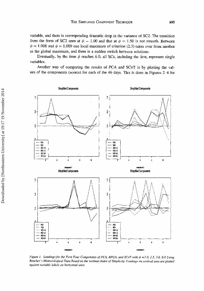
from factor analysis, and proceeds by post-multiplying the (p x m) matrix of PC loadingsby a (usually orthogonal) matrix to make the loadings "simple." Simplicity is definedby one of a number of criteria (e.g., varimax, quartimax) which quantify the idea thatloadings should be near zero or near ±1, with as few as possible intermediate values.Rotation takes place within the subspace defined by the first m PCs. Hence all thevariation in this subspace is preserved by the rotation, but it is redistributed among therotated components, which no longer have the successive maximization property. Weillustrate the procedure with a simple example, given by Rencher (1995), which consistsof 46 daily measurement on 11 meteorological variables. Table 1 lists the variables, andTable 2 and Figure I give loadings for PCs, for rotated PCs, for m = 4, using thewell-known varimax rotation criterion, and for simplified components defined later. Theunrotated analysis has nontrivial loadings on 9 of the 11 variables in its first PC, whichare reduced to 6 after rotation. Similar simplifications occur in later components.
Rotation of principal cOI~ponents has a number of drawbacks (Jolliffe 1987, 1989,1995). We defer detailed discussion of these until later in the article, when we comparethe properties of rotated PCs with the components produced by a new technique. Thissimplified component technique (SCoT) has one stage, rather than the two needed inrotated PCA, and each simplified component optimizes a criterion combining the desirableproperties of large variance and simplicity. Successive components are constrained to beorthogonal to, or uncorrelated with, one another. SCoT is defined in Section 2 andillustrated with examples in Section 3. Comparisons are made with rotated PCA in bothSections 2 and 3. Computational aspects of SCoT are discussed in Section 4. A simulationstudy in which some properties of SCoT are described in Section 5, and further discussionand concluding remarks are given in Section 6.
2. THE SIMPLIFIED COMPONENT TECHNIQUE
2.1 PRINCIPAL COMPONENT ANALYSIS
To establish notation we formally define PCA. Let x be a vector of p randomvariables with covariance matrix ~. The kth principal component, for k = 1, 2, ... .p,
is the linear function of x, a~x, which maximizes var[a~x] = a~~ a k subject toa~ak = 1, and, (for k > 1), a~ak = 0, j < k.
Dow
nloa
ded
by [
Nor
thea
ster
n U
nive
rsity
] at
19:
17 1
9 N
ovem
ber
2014
THE SIMPLIFIED COMPONENT TECHNIQUE 691
Often PCA is done for variables standardized to each have unit variance, so that ~becomes the correlation matrix for the original variables. In practice, we work with a(n x p) data matrix X, and the sample covariance/correlation matrix, S, for these data.We denote the value of the kth PC for the ith observation (row of X) by a~xi in thiscase.
2.2 ROTATION
Suppose that we have decided to retain and rotate m PCs and that A is the (p x m)matrix whose kth column is ak, k = 1,2, ... , m. Rotating the first m components isachieved by post-multiplying A by a matrix T, to obtain rotated loadings B = AT.The choice of T is determined by whichever rotation criterion we use. For example,for the commonly used varimax rotation criterion, T is an orthogonal matrix chosen tomaximize
(2.1)
where bj k is the (j, k)th element of B (Krzanowski and Marriott 1995).The idea behind the varimax criterion is to simplify the structure of the loadings
by maximizing the variance of squared loadings within each column of B. This drivesthe loadings towards zero or ± 1; alternative rotation criteria attempt to achieve similarobjectives, but using a variety of other specific definitions. Concentrating the loadingsclose to zero or ±l is not the only possible definition of simplicity. For example, if allloadings were equal, that is also simple but in a completely different way. Building acriterion to take into account both types of simplicity would be difficult, and hence westick to the usual concept, as typified by varimax.
2.3 THE SIMPLIFIED. COMPONENT TECHNIQUE
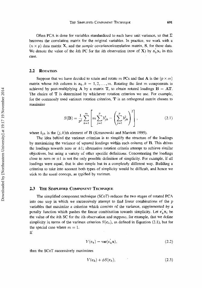
The simplified component technique (SCoT) reduces the two stages of rotated PCAinto one step in which we successively attempt to find linear combinations of the pvariables that maximize a criterion which consists of the variance, supplemented by apenalty function which pushes the linear combination towards simplicity. Let C~Xi bethe value of the kth SC for the ith observation and suppose, for example, that we definesimplicity in terms of the varimax criterion S(Ck), as defined in Equation (2.1), but forthe special case where m = 1.
If
(2.2)
then the SCoT successively maximizes
(2.3)
Dow
nloa
ded
by [
Nor
thea
ster
n U
nive
rsity
] at
19:
17 1
9 N
ovem
ber
2014

692 I. T. JOLLIFFE AND M. UDDIN
subject to C~Ck = 1 and, (for k 2: 2) either C~Ck = 0, or C~SCk = O,j < k. Here ¢ is asimplicity/complexity parameter.
Remark 1. There are links between SCoT and other statistical techniques. Penaltyfunctions have been used in several applications in statistics. In many cases, the penaltyfunction is a roughness penalty, included to increase smoothness (see, e.g., Titterington1985; Rice and Silverman 1991; Green and Silverman 1994) rather than a complexitypenalty which targets simplicity. If ¢ = 0, we simply obtain PCA, while as ¢ -+ 00, wewill eventually get each SC containing only one of the original variables.
There are also connections with projection pursuit. The latter finds "interesting" low(m-) dimensional projections of a high (p-) dimensional dataset. "Interesting" can meana variety of things (Huber 1985; Jones and Sibson 1987), but often indicates structuressuch as clusters or outliers. If "high variance" can be thought of as "interesting," PCA is aspecial case of projection pursuit. Indeed if the main source of variation in a dataset is thatbetween a set of clusters, PCA will find such clusters. Huber (1985) suggested that sometypes of factor analysis are also special cases of projection pursuit. However, the rotationassociated with factor analysis is concerned with simplifying the interpretation of the axesdefining the m-dimensional projections, rather than seeking projections with interestingstructures. Morton (1989) modified projection pursuit by incorporating a penalty functionbased on a simplicity index, and it is this approach, in the context of PCA, that we haveadopted.
Remark 2. The one-step procedure of SCoT cannot give equivalent results totwo-stage rotated PCA. The rotated PCs remain within the subspace obtained by them retained PCs; that is, the m-dimensional subspace with maximum variance. The introduction of the penalty function necessarily takes us outside this subspace, so SCoTsacrifices some variance in its search for simplicity. There is no obvious sense in whichthe m-dimensional space defined by SCs is globally optimal.
Remark 3. The one-step procedure operates successively, so a decision to increasethe number of retained components from m to m + 1 leaves the first m componentsunchanged. With rotated PCs a change from m to m + 1 may change the nature of allthe rotated PCs.
Remark 4. Computationally, finding PCs followed by rotation is straightforward.This is especially helped by PCA reducing to an eigenanalysis for which efficient algorithms are readily available. The optimization problem defined by SCoT is more complex.Details of our computational procedures and experience are described in Section 4.
Remark 5. To ensure that successive SCs are different from each other we haveimposed the orthogonality constraints C~Ck = 0, j < k, or the constraints C~SCk =
0, j < k, which mean that the SCs are pairwise uncorrelated. For PCA the constraintsa~ak = °and a~Sak = °are equivalent, but after rotation at least one of these twoproperties (orthogonality or uncorrelatedness) is lost (Jolliffe 1995). Similarly, with SCoTwe cannot keep both properties. Results for each set of constraints are discussed for theexamples which follows.
Dow
nloa
ded
by [
Nor
thea
ster
n U
nive
rsity
] at
19:
17 1
9 N
ovem
ber
2014

3.1 EXAMPLE 1
THE SIMPLIFIED COMPONENT TECHNIQUE
3. EXAMPLES
693
3.1.1 Simplified Components With Orthogonality
Returning to the example introduced in Section 1, we first use SCoT with the orthogonality constraints, C~Ck = 0, j < k. Table 2 and Figure 1 give loadings of the first fourcomponents for PCA, for rotated PCA (RPCA) and for SCoT with ¢ = 1.00, 1.50,3.0,and 6.0. For ¢ = 1.00 the first SC is very similar to the first PC, though slightly simpler.The second SC is intermediate in simplicity to the second PC and to the second RPC,though "second" has no clear meaning in the case of RPCA. The third and fourth SCsare simpler than either the corresponding PC or RPC.
Table 2. Loadings for the PCA, for RPCA, and for SCoT with varying values of ¢, for Rencher'smeteorological data.
Component (1) (2) (3) (4)
Technique variable Loading matrix
PCA X1 .33 .08 -.09 -.28(= SCoT X2 .35 - .19 -.11 -.23
with X3 .39 -.05 -.11 -.14¢ = 0) X4 .38 -.05 -.13 -.01
Xs .23 -.53 -.01 -.07X6 .36 -.24 -.12 .13X7 -.09 -.02 -.79 .54Xs -.25 -.50 -.08 -.15Xg -.31 -.36 -.21 -.23
X10 -.02 -.47 .47 .50X11 .34 .11 .18 .45
RPCA X1 .36 .05 -.12 .23X2 .46 -.10 -.07 .03X3 .43 .05 -.02 .06X4 .39 .10 .08 -.00Xs .39 -.30 -.03 -.31X6 .38 .03 .16 -.21X7 -.01 -.03 .96 .03Xs -.01 -.56 .00 -.17Xg -.05 -.56 .06 .04
X10 -.13 .02 -.06 -.82X11 .09 .50 .10 -.32
SCoT X1 -.33 -.06 .02 -.03(¢ = 1.00) X2 -.35 .15 .03 -.11
X3 -.40 .03 .04 -.06X4 -.39 .03 .06 -.04Xs -.23 .60 .01 -.24X6 -.36 .19 .07 -.06X7 .08 .01 .99 .08Xs .24 .51 -.01 -.27Xg .31 .31 .02 -.22
XlO .02 .45 -.08 .87X11 -.33 -.09 .01 .18
Dow
nloa
ded
by [
Nor
thea
ster
n U
nive
rsity
] at
19:
17 1
9 N
ovem
ber
2014

694 I. T. JOLLIFFE AND M. UDDIN
Table 2. Continued
Component (1) (2) (3) (4)
Technique variable Loading matrix
SCoT X1 -.33 -.04 .01 .06(¢=1.50) X2 -.36 .04 .04 .14
x3 -.40 .00 .04 .10x4 -.39 .00 .05 .10Xs -.22 .17 .04 .21xa -.36 .07 .07 .14X7 .08 -.04 .99 -.05xa .24 .13 .02 .92Xg .30 .07 .03 .09XlO .02 .97 .02 -.19X11 -.33 .01 .01 -.02
SCoT x1 -.32 .01 -.02 .07(¢ = 3.00) X2 -.36 -.02 -.03 .04
x3 -.41 -.00 -.03 .07x4 -.40 -.00 -.04 .07Xs -.22 -.08 -.02 -.96xa -.37 -.03 -.05 .03X7 .08 .02 -1.00 .01Xa .23 -.06 .00 -.14Xg .30 -.03 -.00 -.13
X10 .02 -.99 -.02 .08x1j -.33 -.02 -.02 .10
SCoT X1 .09 -.03 .01 -.01(¢ = 6.00) x2 .10 -.03 -.00 -.01
X3 .97 .10 -.01 .02X4 .10 -.04 .00 -.00Xs .06 -.02 -.03 -.00xa .09 -.04 -.01 .00X7 -.02 .01 .01 1.00xa -.06 .04 -.03 .01Xg -.07 .05 -.02 .02xlO -.01 -.00 -1.00 .01X12 .08 -.99 .00 .02
These changes in simplicity are quantified in Table 3, as are the changes in variance.At ¢J = 1.00 the third SC is almost as simple as it can be, with its varimax value close to1. SC4, although less simple, has one loading much larger than all others. By contrast,SC2, although simpler than PC2, still has nontrivial loadings on four variables. In termsof simplicity, as measured by the varimax criterion, SC2 is almost as good as RPC2. Itsvariance is less than that of RPC2, but this is expected because SCI accounts for a muchgreater proportion of variance than RPC1. The total variance accounted for by the firsttwo SCs is only slightly less than for the first two PCs. SC2 is a simplified version of PC2,and SC2 has high loadings on a slightly different set of variables compared to RPC2evaporation (RPC2) is replaced by total wind (SC2) and minimum soil temperaturebecomes more important (SC2) at the expense of integrated area under the daily humiditycurve. These different groupings may provide different insights into the structure of thedataset.
As ¢J increases from 1.00 to 1.50, SC2 in tum becomes dominated by a single
Dow
nloa
ded
by [
Nor
thea
ster
n U
nive
rsity
] at
19:
17 1
9 N
ovem
ber
2014
THE SIMPLIFIED COMPONENT TECHNIQUE 695
variable, and there is corresponding dramatic drop in the variance of SC2. The transitionfrom the form of SC2 seen at ¢ = 1.00 and that at ¢ = 1.50 is not smooth. Between¢ = 1.008 and ¢ = 1.009 one local maximum of criterion (2.3) takes over from anotheras the global maximum, and there is a sudden switch between solutions.
Eventually, by the time ¢ reaches 6.0, all SCs, including the first, represent singlevariables.
Another way of comparing the results of PCA and SCoT is by plotting the values of the components (scores) for each of the 46 days. This is done in Figures 2--4 for
- PCI- RC1-.--- SC1l.0--_. SCI1.5--- SCl~O
- SCl6D
~\! \! \! \
Sim~ified Components
00l1lpCIfI0lI1
Sim~ified Components
10
- PC2-RC:!-•••• SC21.0--_. 5121.5-_. SC23.0-5126.0
Simplified Components
""""",,12
Sim~ified Components
10
- PC3- RC3----- 5C31.0--_. 5C315--- 5C3~0
- 5C3ao
10
- PC4- Rei.-••• 5C41.0--_. 5C4f.5-_. 5C4aG
- 5C4ao
10
Figure 1. Loadings for the First Four Components ofPCA, RPCA, and SCoT with rj; =1.0, 1.5, 3.0, 6.0 UsingRencher's Meteorological Data Based on the varimax Index of Simplicity. Loadings on vertical axes are plottedagainst variable labels on horizontal axes.
Dow
nloa
ded
by [
Nor
thea
ster
n U
nive
rsity
] at
19:
17 1
9 N
ovem
ber
2014
696 I. T. JOLLIFFE AND M. UDDIN
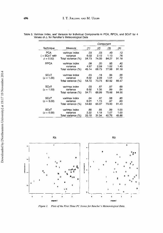
Table 3. Varimax Index, and Variance for Individual Components in PCA, RPCA, and SCoT for 4Values of ¢, for Rencher's Meteorological Data
Component
Technique Measure (1) (2) (3) (4)
PCA varimax index .03 .03 .40 .12(= SCoT with variance 6.02 2.12 1.13 .76
¢ = 0.00) Total variance (%) 54.73 74.00 84.27 91.18
RPCA varimax index .08 .20 .85 .42variance 4.97 2.59 1.02 1.45
Total variance (%) 45.14 68.73 77.98 91.18
SCoT varimax index .03 .18 .96 .55(¢ = 1.00) variance 6.02 2.09 1.01 .72
Total variance (%) 54.72 73.73 82.92 89.47
SCoT varimax index .03 .87 .97 .69(¢ = 1.50) variance 6.02 1.35 .99 .94
Total variance (%) 54.71 66.99 75.98 84.50
SCoT varimax index .04 .97 .98 .85(</> = 3.00) variance 6.01 1.15 .97 .83
Total variance (%) 54.63 65.07 73.90 81.43
SCoT varimax index .88 .95 .99 1.00(¢ = 6.00) variance 2.22 1.19 1.07 1.00
Total variance (%) 20.19 31.04 40.76 49.86
PeA peA
34
12363841 43 12
38 2\
\118
21 15 7119 23N • 16 31 35 '!li E19 '!l ~46 ~
40
& 25 484243124445 ~ 0
17
L 20 22 35 :!l 9 \8 1316331 ~
8\5
21713822 42 29
33!l
4514 39 44
4024
12 1(1
12 33 II41
1013 39
11~
10
·2 -6 ~ ·2
_11 componenll
Figure 2. Plots of the First Three PC Scores for Rencher's Meteorological Data.
Dow
nloa
ded
by [
Nor
thea
ster
n U
nive
rsity
] at
19:
17 1
9 N
ovem
ber
2014

THE SIMPLIFIED COMPONENT TECHNIQUE 697
components 1 to 3. From Figures 2--4, we see that for small values of rjJ, the plots forSCoT are similar, apart from some sign changes, to those of PCA, but as expected thereis greater divergence for large values of rjJ. The pattern which is apparent in SC3 for¢ = 3.0 is because this component is dominated by variable 7 which takes only a fewdiscrete values.
Rotated components are not plotted. In four-dimensional space, the configuration ofthe points will be the same as that of PCA, but will be rotated. Because of the arbitrarinessof the labeling of the RPCs, it is not meaningful to compare their plots, 2 componentsat time, with those of PCA and SCoT.
SCoT 1.0
11
13 10
12 41
4039 14
3627i4 3315
~ 03/3 ~ 1635 Z!
! 45U 4342:al
& ~ '!I'IB 19E8
1821 17
36
SCoT 1.0
34
36
:al
:j!i; 2843
" - 21
"13.s:
&'!I27~! 23
40 4114 1~79 15 18
I48
122442 Z! 31II 3218
3 4
J;454410 335
·2
compcnenll
SCoT 1.5
34
36
:al
~'lB43 13
217 6
'!I27
:ll1 23 40 N 9
1~7 1516
48 12 112442 Z! 31218
~45443
4
1033
5
_II
Figure 3. Plots of the First Three SC Scores with <P = I.O,l.5for Rencher's Meteorological Data Based on thevarimax Index ofSimplicity.
Dow
nloa
ded
by [
Nor
thea
ster
n U
nive
rsity
] at
19:
17 1
9 N
ovem
ber
2014

698 I. T. JOLLIFFE AND M. UDDIN
3.1.2 Simplified Components Keeping Uncorrelatedness
It was noted in Section 2.3 that, unlike PCA, we cannot achieve both uncorrelatedness and orthogonality between the simplified components. In this section we report theresults for the meteorological data when uncorrelatedness, rather than orthogonality, isimposed. Table 4 gives loadings, simplicity factors and variances for the first four SCswhen 1> = 1.0. Comparisons with Tables 2-3 show that there is little difference from theorthogonal SCs. The first SC is necessarily the same for both sets of components. As
SCoT 3.0 SCoT 3.0
21 I~ 3352
311 4544 1029
253145 311 17 34
4526 43 15 1110 31215
M35 23 I 45 122442 IP
2230 1I 41 4
11 1542 3III I~~
N34 • 2340
i 25 i 3711_
~ ~ 7 5
E 24 40 33 32 ~ 218;ii2843 13
39 1420
12311
11 10
13 34
·2
COOlponenll COOlponenll
SCoT 6.0 SCoT 6.0
5 41 15 I~I7 29
2831 46
15 15 17 43 ~2016 15 23 35 443735
20
3133
I H 1I4 42 30
32 40 3 34N 19
i 25
~ d5E 40248 32 33
21 10 23 14 39
5 .p 1214 1134
1342 35213271244 45
3022 372946
10 II
24 31139 13
·3 ·3 ·2
COOlponenll _11
Figure 4. Plots of the First Three SC Scores with ¢ =3.0,6.0 for Rencher's Meteorological Data Based on thevarimax Index of Simplicity.
Dow
nloa
ded
by [
Nor
thea
ster
n U
nive
rsity
] at
19:
17 1
9 N
ovem
ber
2014

THE SIMPLIFIED COMPONENT TECHNIQUE 699
Table 4. Simplified Loadings for Rencher's (1995) Meteorological Data Using Uncorrelated SCoTwith ¢ = 1.0
BC (1) (2) (3) (4)variables Loading matrix
X1 .33 .07 -.03 .93X2 .35 -.15 -.03 -.08X3 040 -.03 -.04 -.09X4 .39 -.03 -.06 -.12Xs .23 -.61 -.01 -.02xa .36 -.19 -.07 -.12X7 -.08 -.01 -.99 -.00xa -.24 -.51 .01 .12Xg -.31 -.31 -.02 .17
XlO -.02 -AS .08 -.01X11 .33 .09 -.01 -.19
Simplicity factor .03 .18 .96 .74Total Variance (%) 54.72 73.73 82.91 86.64
¢ increases, the second uncorrelated SC is very similar to the second orthogonal SCuntil ¢ = 4.0. As ¢ increases from 4.0, the rate of decrease in variance is slightlyhigher in the uncorrelated SC than in the orthogonal Sc. On the other hand, the seconduncorrelated SC achieves greater simplicity than the second orthogonal SC. For SC3 theuncorrelated component has slightly higher variance than the orthogonal component. The.fourth uncorrelated component has a higher rate of decrease in variance than that obtainedby keeping orthogonality. In contrast to orthogonal SCoT, uncorrelated SCoT will notproduce all components equivalent to single variables as ¢ increases (unless the variablesthemselves are uncorrelated). Tables 3-4 show that SCoT (with either orthogonality anduncorrelatedness) simplifies the components better than RPCA in terms of the varimaxcriterion. The first four uncorrelated SCs account for 86.64% of the total variance, aroughly 3% reduction in variance compared to orthogonal SCoT, but with a gain insimplicity for SC4. The first three SCs are very similar and, on the whole, the twoapproaches of the SCoT, keeping orthogonality and maintaining uncorrelatedness, capturesimilar patterns among the retained sets of the loading matrices. This is not particularlysurprising, as orthogonal SCoT produced only slightly correlated components for thisexample (Table 5). Similarly, the uncorrelated SCoT gives a nearly orthogonal set ofvectors.
Table 5. Correlation Matrix for the First Four Orthogonal Simplified Components with ¢ = 1.0 forRencher's Meteorological Data
Correlation Matrix
Components (1) (2) (3) (4)
(1) 1.00 .00 -.01 .00(2) 1.00 .01 .03(3) 1.00 -.21(4) 1.00
Dow
nloa
ded
by [
Nor
thea
ster
n U
nive
rsity
] at
19:
17 1
9 N
ovem
ber
2014

700 I. T. JOLLIFFE AND M. UDDIN
Table 6. Simplified Loadings for Rencher's Meteorological Data Using SCoT with Variable if;(5.0,1.0,.0001,.0001) Along the First Four Dimensions
SC (1) (2) (3) (4)variables Loading matrix
X1 .31 -.07 -.07 .27X2 .35 .14 -.10 .22X3 .47 .03 -.11 .14X4 .41 .03 -.12 .01Xs .20 .58 -.01 .06x6 .36 .18 -.11 -.14X7 -.07 .01 -.79 -.55X8 -.21 .53 -.11 .16Xg -.28 .32 -.24 .23XlO -.02 .45 .45 -.49X11 .31 -.10 .21 -.46
Simplicity factor .05 .17 .39 .13Total Variance (%) 54.13 73.22 83.58 90.50
3.1.3 Simplified Components with Variable <jJ
The behavior in this, and other, examples indicates that if we take <jJ large enoughfor SCI to become noticeably different from PCI, all the subsequent SCs are oftendominated by single variables. Allowing the possibility of using different values of <jJ fordifferent SCs may avoid this and will increase flexibility. A smaller value of <jJ will beused in deriving SC2 than for SCI, a still smaller value for SC3 and so on.
Table 6 gives results for the meteorological data set with <jJ = (5.0,1.0, .0001, .0001).As before, the transition between different patterns in the SCs with the increase in <jJ isnot at all smooth, and to obtain a compromise for all SCs between closeness to PCAand domination by a single variable, the values of <jJ for different SCs are very different.Compared to PCA, the third and fourth components now gain only a very small amountof simplicity at the cost of losing a small amount of variance (about 1%) along theretained set of first four components. For this reason the retained components are nearlyuncorrelated and remain close to PCA (Tables 2, 6, and 7).
Table 7. Correlation Matrix for the First Four Orthogonal Simplified Components for Rencher's Meteorological Data Using SCoT with Variable if; = (5.0,1.0,.0001,.0001) Along the First FourDimensions
Correlation matrix
Components (1) (2) (3) (4)
(1) 1.00 -.03 .08 -.03(2) 1.00 -.02 -.00(3) 1.00 .00(4) 1.00
Dow
nloa
ded
by [
Nor
thea
ster
n U
nive
rsity
] at
19:
17 1
9 N
ovem
ber
2014

THE SIMPLIFIED COMPONENT TECHNIQUE
Table 8. Definitions of Variables in Jarvik's Smoking Questionnaire
Variable Definition
X1 ConcentrationX2 Annoyancex3 Smoking 1 (first wording)X4 SleepinessXs Smoking 2 (second wording)X6 TensenessX7 Smoking 3 (third wording)xa AlertnessXg Irritability
x10 TirednessX11 ContentednessX12 Smoking 4 (fourth wording)
3.2 EXAMPLE 2
701
The data analyzed in this section are from Jarvik's smoking questionnaire (M. E.Jarvik, unpublished). The data involve the answers by 110 individuals to 12 questions,listed in Table 8, each coded from 1 to 5 such that a high score represents a desire tosmoke. The four questions labeled "smoking" are direct questions about the subject'sdesire to have a cigarette. The remainder of the questions relate to the psychological andphysical state of the subjects.
Figure 5 gives loadings for PCA, for RPCA, and for SCoT with a range of valuesof ¢, and Table 9 contains information on the variances and the values of the varimaxcriterion for each component in Figure 5. The behavior seen in Figure 5 and Table 9 issimilar to that in Figure 1 and Table 3. The first SC remains similar to PC1 until ¢ isquite large, and as ¢ increases SC3, then SC2 and finally SCI becomes dominated by asingle variable.
Examining, for example, SCoT when ¢ = 2.0 we find that SCI is still close toPC1 and SC3 is dominated by a single variable, Smoking 1 (First wording). SC2 hasits highest loadings on the same four variables as RPCA but is simpler in the sense thatone variable (contentedness) plays a much more dominant role compared to other threevariables than in RPCA. Compared to PCA, the first two SCs lose 9%, while RPCA loses18%. With three components, where RPCA necessarily retains the same total variabilityas PCA, SCA loses 13% but with a considerable gain in simplicity.
4. SIMULATION STUDIES
One question of interest is whether SCoT is better at detecting underlying simplestructure in a dataset when it exists than is PCA or RPCA. To investigate these questionswe simulated data from a variety of known structures. Only a small part of the results isgiven here; further details can be found in Uddin (1999).
Dow
nloa
ded
by [
Nor
thea
ster
n U
nive
rsity
] at
19:
17 1
9 N
ovem
ber
2014

702 I. T. JOLLIFFE AND M. UDDIN
4.1 STRUCTURE OF THE SIMULATED DATA
Given a vector l of positive real numbers and an orthogonal matrix A, we can attemptto find a covariance matrix or correlation matrix whose eigenvalues are the elements ofl, and whose eigenvectors are the columns of A. Some restrictions need to be imposedon l and A, especially in the case of correlation matrices, but it is possible to findsuch matrices for a wide range of eigenvector structures. Having obtained a covarianceor correlation matrix it is straightforward to generate samples of data from multivariate
- PCI_ .•- RCI••••• SC1~0
--- SCI ao-_. SC16.0
Sim~ified Components
J'1\1\I \I \I \
r. I \ '\I --'
component 1
- PC!- RC3..... SC32.0---- SC330-_. SC36.0
10
-PC:1-- RI:1..... S1:12.0---- 51:13.0-_. SI:1M
Simplified Components
"", \1\, ,
I \, \I \, \
I \, ,I \, ,
I \, \
10
Sim~ified Components
C01IJlClIOll2
10
Figure 5. Loadings for the First Three Components of PCA, RPCA, and SCoT with ¢> =2.0, 3.0, 6.0 usingJarvik's Smoking Data Based on the varimax Index ofSimplicity. Loadings on vertical axes are plotted againstvariable labels on horizontal axes.
Dow
nloa
ded
by [
Nor
thea
ster
n U
nive
rsity
] at
19:
17 1
9 N
ovem
ber
2014
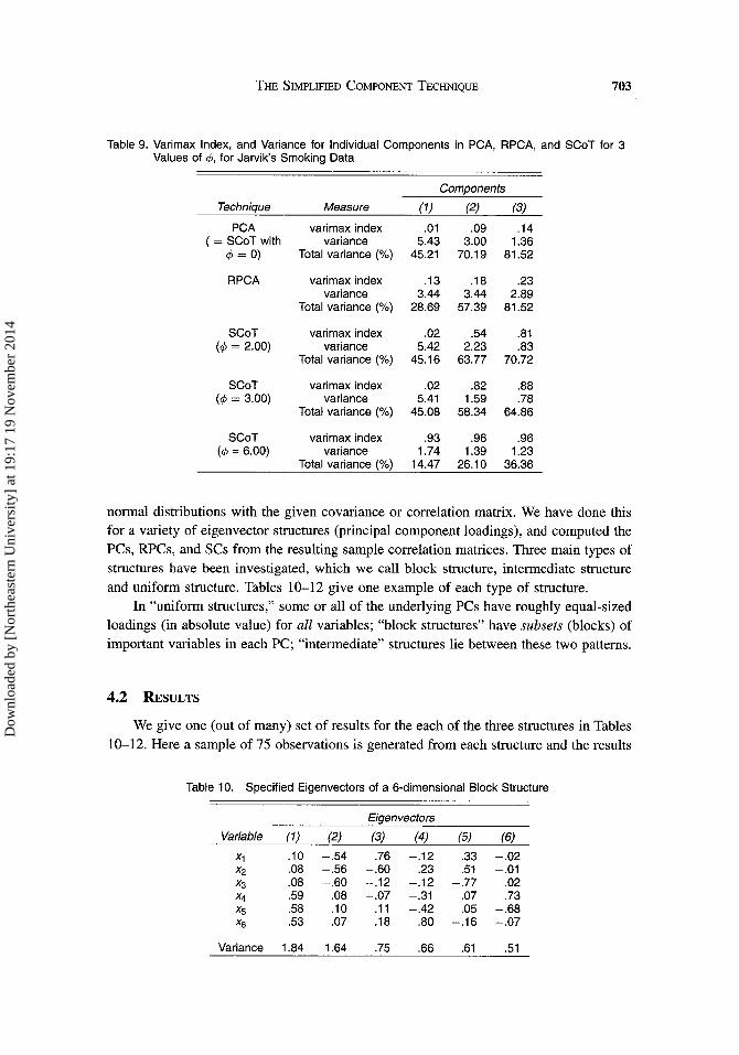
THE SIMPLIFIED COMPONENT TECHNIQUE 703
Table 9. Varimax Index, and Variance for Individual Components in PCA, RPCA, and SCoT for 3Values of </>, for Jarvik's Smoking Data
Components
Technique Measure (1) (2) (3)
PCA varimax index .01 .09 .14(= SCoT with variance 5.43 3.00 1.36
</>= 0) Total variance (%) 45.21 70.19 81.52
RPCA varimax index .13 .18 .23variance 3.44 3.44 2.89
Total variance (%) 28.69 57.39 81.52
SCoT varimax index .02 .54 .81(</> = 2.00) variance 5.42 2.23 .83
Total variance (%) 45.16 63.77 70.72
SCoT varimax index .02 .82 .88(</> = 3.00) variance 5.41 1.59 .78
Total variance (%) 45.08 58.34 64.86
SCoT varimax index .93 .96 .96(</> =6.00) variance 1.74 1.39 1.23
Total variance (%) 14.47 26.10 36.36
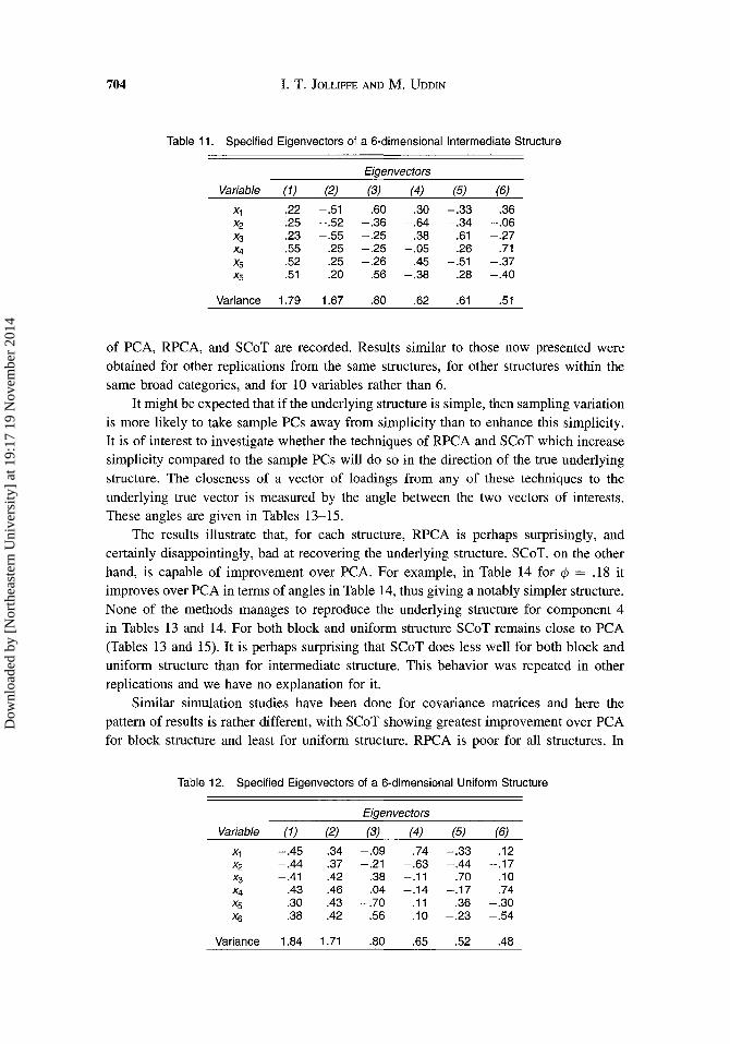
normal distributions with the given covariance or correlation matrix. We have done thisfor a variety of eigenvector structures (principal component loadings), and computed thePCs, RPCs, and SCs from the resulting sample correlation matrices. Three main types ofstructures have been investigated, which we call block structure, intermediate structureand uniform structure. Tables 10-12 give one example of each type of structure.
In "uniform structures," some or all of the underlying PCs have roughly equal-sizedloadings (in absolute value) for all variables; "block structures" have subsets (blocks) ofimportant variables in each PC; "intermediate" structures lie between these two patterns.
4.2 RESULTS
We give one (out of many) set of results for the each of the three structures in Tables10-12. Here a sample of 75 observations is generated from each structure and the results
Table 10. Specified Eigenvectors of a 6-dimensional Block Structure
Eigenvectors
Variable (1) (2) (3) (4) (5) (6)
x1 .10 -.54 .76 -.12 .33 -.02X2 .08 -.56 -.60 .23 .51 -.01X3 .08 -.60 -.12 -.12 -.77 .02X4 .59 .08 -.07 -.31 .07 .73Xs .58 .10 -.11 -.42 .05 -.68Xs .53 .07 .18 .80 -.16 -.07
Variance 1.84 1.64 .75 .66 .61 .51
Dow
nloa
ded
by [
Nor
thea
ster
n U
nive
rsity
] at
19:
17 1
9 N
ovem
ber
2014
704 I. T. JOLLIFFE AND M. UDDIN
Table 11. Specified Eigenvectors of a 6-dimensional Intermediate Structure
Eigenvectors
Variable (1) (2) (3) (4) (5) (6)
x1 .22 -.51 .60 .30 -.33 .36X2 .25 -.52 -.36 -.64 -.34 -.06X3 .23 -.55 -.25 .38 .61 -.27X4 .55 .25 -.25 -.05 .26 .71Xs .52 .25 -.26 .45 -.51 -.37Xs .51 .20 .56 -.38 .28 -.40
Variance 1.79 1.67 .80 .62 .61 .51
of PCA, RPCA, and SCoT are recorded. Results similar to those now presented wereobtained for other replications from the same structures, for other structures within thesame broad categories, and for 10 variables rather than 6.
It might be expected that if the underlying structure is simple, then sampling variationis more likely to take sample PCs away from simplicity than to enhance this simplicity.It is of interest to investigate whether the techniques of RPCA and SCoT which increasesimplicity compared to the sample PCs will do so in the direction of the true underlyingstructure. The closeness of a vector of loadings from any of these techniques to theunderlying true vector is measured by the angle between the two vectors of interests.These angles are given in Tables 13-15.
The results illustrate that, for each structure, RPCA is perhaps surprisingly, andcertainly disappointingly, bad at recovering the underlying structure. SCoT, on the otherhand, is capable of improvement over PCA. For example, in Table 14 for ¢ = .18 itimproves over PCA in terms of angles in Table 14, thus giving a notably simpler structure.None of the methods manages to reproduce the underlying structure for component 4in Tables 13 and 14. For both block and uniform structure SCoT remains close to PCA(Tables 13 and 15). It is perhaps surprising that SCoT does less well for both block anduniform structure than for intermediate structure. This behavior was repeated in otherreplications and we have no explanation for it.
Similar simulation studies have been done for covariance matrices and here thepattern of results is rather different, with SCoT showing greatest improvement over PCAfor block structure and least for uniform structure. RPCA is poor for all structures. In
Table 12. Specified Eigenvectors of a 6-dimensional Uniform Structure
Eigenvectors
Variable (1) (2) (3) (4) (5) (6)
X1 -.45 .34 -.09 .74 -.33 .12X2 -.44 .37 -.21 -.63 -.44 -.17X3 -.41 .42 .38 -.11 .70 .10X4 .43 .46 .04 -.14 -.17 .74Xs .30 .43 -.70 .11 .36 -.30Xe .38 .42 .56 .10 -.23 -.54
Variance 1.84 1.71 .80 .65 .52 .48
Dow
nloa
ded
by [
Nor
thea
ster
n U
nive
rsity
] at
19:
17 1
9 N
ovem
ber
2014

THE SIMPLIFIED COMPONENT TECHNIQUE 705
Table 13. Angles Between the Underlying Vectors and the Sample Vectors of PCA, RPCA, and SCoTwith Various Values of cP, for a Specified Block Structure of Correlation Eigenvectors
Vectors
Technique cP (1) (2) (3) (4)
PCA 0 12.9 12.0 15.4 79.5
RPCA 37.7 45.2 45.3 83.1
SCoT .11 12.5 11.8 15.7 70.6.18 12.4 11.9 17.0 69.3.25 12.2 12.2 19.4 68.8.33 12.1 13.0 23.8 68.9.43 12.0 15.0 31.6 69.6
both correlation and covariance simulations much smaller values of ¢, compared to thoseused in the examples of Section 3, are needed to show improvement for SCoT over PCA.We return to this point in Section 6.
Finally in this section, we note that comparisons of underlying and sample structures are complicated by switching of the order of the first two components in somereplications. This switching may occur because of a change of signs in some blockswithin the population and sample correlation or covariance matrices, and is sometimesdue to the closeness of the first two population eigenvalues; there are occasions whenboth phenomena are present.
5. COMPUTATION
5.1 OPTIMIZATION
The simplified component technique relies on numerical optimization to estimateparameters and it suffers from the problem of many local optima. Traditional methodsof function optimization can have considerable difficulty in converging to the globaloptimum when multiple optima are present, as is the case here. In contrast to traditional
Table 14. Angles Between the Underlying Vectors and the Sample Vectors of PCA, RPCA, and SCoTwith Various Values of cP, for a Specified Intermediate Structure of Correlation Eigenvectors
Vectors
Technique cP (1) (2) (3) (4)
PCA 0 13.7 15.1 23.6 78.3
RPCA 53.3 42.9 66.4 77.7
SCoT .05 10.7 12.5 22.7 77.8.11 6.3 9.2 21.4 76.9.18 6.4 9.2 19.8 75.2.25 10.0 12.0 17.5 71.3.33 13.2 14.8 15.9 66.1.43 16.2 17.6 21.7 64.1
Dow
nloa
ded
by [
Nor
thea
ster
n U
nive
rsity
] at
19:
17 1
9 N
ovem
ber
2014

706 I. T. JOLLIFFE AND M. UDDIN
Table 15. Angles Between the Underlying Vectors and the Sample Vectors of PCA, RPCA, and SCoTwith Various Values of cP, for a Specified Uniform Structure of Correlation Eigenvectors
Vectors
Technique cP (1) (2) (3) (4)
PCA 0 6.0 6.4 23.2 31.8
RPCA 52.0 54.1 39.4 43.5
SCoT .11 6.0 6.7 21.5 24.9
.18 6.1 6.9 21.3 22.5
.25 6.2 7.2 21.7 21.4
.33 6.2 7.5 22.5 22.4
.43 6.4 8.0 23.9 26.1
optimization methods, simulated annealing is less likely to fail in finding the globaloptima of a multidimensional function (Lundy and Mees 1986; Mitra, Romeo, andSangiovanni-Vincentelli 1986; Goffe, Ferrier, and Rogers 1994). However, the maindrawback of the simulated annealing method, which has limited its use, is that convergence can be very slow. These algorithms can be speeded up, but at the expense of notalways finding a global optimum.
For the case of multiple optima, a common approach is to run traditional routinesfrom a number of starting points and to choose the best solution from those obtained. Themain difficulty with this approach arises with the choice of starting points as traditionalmethods are sensitive to the starting points. Since we have no a priori knowledge ofthe p-dimensional surface, this choice is arbitrary and has a considerable effect upon thereliability and efficiency of the algorithm. However, reliability can be achieved to someextent by iterating the underlying function for a sufficient number of times for differentwell-spaced starting points.
In this study, we developed a new technique which produces a set of simplifiedcomponents. In this technique, we used the built-in quasi-Newton function of S-Plus,interfaced with the modified FORTRAN functions based on dmnfb, dmngb, and dmnhb(Gay 1983, 1984). The modified FORTRAN functions were used for both constrainedand unconstrained maximization in the proposed S-Plus code of SCoT, and depend onwhether we used variable or fixed ¢. To achieve an appropriate solution, several differentrandom starting points were used along each dimension and the quasi-Newton methodwas applied. The maximum value of the objective function defined in (2.3) and thecorresponding vectors thus obtained were selected.
To ensure the criterion values for SCI, SC2, SC3, ... were in decreasing order, andto ensure that all the maxima were global maxima, the problem was solved by replicatingthe optimization 11 times, with different randomly chosen unit vectors and for differentstarting values. Adopting this strategy, the convergence is quicker than the simulatedannealing method.
Dow
nloa
ded
by [
Nor
thea
ster
n U
nive
rsity
] at
19:
17 1
9 N
ovem
ber
2014

5.2 ORTHOGONALITY
THE SIMPLIFIED COMPONENT TECHNIQUE 707
Another important aspect of the SCoT is the implementation of orthogonality or
uncorrelatedness. In the sequential approach of PCA, orthogonality between the suc
cessive vectors (a., al, ... , am) can be maintained by adjusting the matrix of residualcorrelations or variances and covariances.
In SCoT, the Gram-Schmidt process of orthogonalization was used during the max
imization so that the successive vectors (CI' Cl, ... ,cm ) were orthogonal. We find the
first vector CI after maximizing the objective function defined in (2.3). The successive
vectors Ck were obtained by spinning arbitrarily chosen vectors O-k under maximizationby using the transformation
Cl
(5.1)
where the first vector CI was considered as fixed, in finding the successive set of vectors
during the Gram-Schmidt orthogonalization. For each Ck. k 2': 2, each iteration within
the quasi-Newton method is followed by a Gram-Schmidt orthogonalization step.
5.3 UNCORRELATEDNESS
The procedure described in Section 5.2 can be adapted to ensure uncorrelatedness,
rather than orthogonality, between SCs. In this case we require the constraints c~SCk = 0,
hi- k, instead of C~Ck = °for orthogonality.To maintain uncorrelatedness between the SCs, the Gram-Schmidt process of or
thogonalization can once again be used. The condition C~SCk = 0, is equivalent to
Y~Yk = 0, where Y«, k = 1,2, ... is the kth SC, defined as Yi« = XCk, where X is the(n x p) column-centered matrix of the n observations on p variables. Hence C~SCk = °is equivalent to "orthogonality" between Yh and Yk.
We first find the vector CI by maximizing the objective function defined in (2.3),
and this yields the first SC, YI = XCI.
The successive SCs are obtained by spinning the arbitrarily chosen components (k =XO- k (based on the arbitrarily chosen vectors O-k) under maximization by using the transformation
Dow
nloa
ded
by [
Nor
thea
ster
n U
nive
rsity
] at
19:
17 1
9 N
ovem
ber
2014

708
Y2
Y3
Yk
I. T. JOLLIFFE AND M. UDDIN
(5.2)
where the first SC, Yl, is kept fixed. The vectors corresponding to the uncorrelated:I 1 I
components are extracted by the back transformation Ck = (X X)- X Yk. The selectedvectors Ck'S have then been normalized so that they are of unit length. For each Yb
k ~ 2, each iteration within the quasi-Newton method is followed by a Gram-Schmidtorthogonalization step which brings uncorrelatedness between the successive SCs.
6. DISCUSSION AND CONCLUSION
The results of Section 3, and other examples we have examined, show a commonpattern of behavior of SCoT. The simplified components are necessarily close to principalcomponents for small ¢, and as ¢ increases so individual components become dominatedby single variables. Lower-variance components tend to take this simpler form for smallervalues of ¢ than higher-variance components. Transition between different solutions as¢ increases can be sudden, corresponding to switching between different local maximain the optimization problem. This is noted in the discussion of Example 1, and similarbehavior occurs for SCI in Example 2 between ¢ = 5.40 and ¢ = 5.41. The transitionto a dominant-single-variable SC2 appears much smoother in Example 2, but even herewe switch minima as SC3 goes from being dominated by X3 to dominance by X9, as thelatter's contribution to SC2 become smaller.
Despite a tendency for SCs to remain close to PCs or become dominated by a singlevariable, there are typically some values of ¢ for which some SCs have loadings whichare different from the PCs and the RPCs, without becoming single-variable components,and without sacrificing a great deal of variance. Such simplified components can givenew insights into the underlying structure of the data.
Our examples used correlation matrices, but there is no reason why SCoT should notbe used on covariance matrices. The fact that covariance matrix analysis only makes sensewhen all variables are measured in the same units with a relatively small spread in theirvariance, means that covariance matrix analyses are much less common than correlationanalyses. We have, however, examined SCoT in this context. The results are generally inline with expectation. When variances are roughly equal, there is little difference fromthe correlation matrix results. As the variances become increasingly different, the earlyPCs become dominated by single, high variance, variables, so that SCoT does little tochange PCA.
Dow
nloa
ded
by [
Nor
thea
ster
n U
nive
rsity
] at
19:
17 1
9 N
ovem
ber
2014
THE SIMPLIFIED COMPONENT TECHNIQUE 709
A question which arises in a covariance matrix analysis is whether, and how, to"standardize" ¢ so that similar values are relevant to analyses with very different diagonalelements in the covariance matrix. An intuitive idea is to multiply the variance term, thefirst part of the objective function defined in (2.3), by a factor p/trace(S), so that this parthas the same range of values as for a correlation matrix of the same dimension, p. Othermodifications to (2.3) are also possible for both correlation and covariance matrices. Wecould simply divide the first term by trace(S), which equals p for correlation matrices.Alternatively we could express (2.3) as a weighted average 'l/JV(Ck) + (1 - 'l/J)S(Ck),of V(Ck) and S(Ck)' Another variation of the technique would be to maximize V(Ck)subject to S(Ck) = T, for some fixed T, a form of PCA with constraints. This will giveus SCI, but later components will be SCs with a particular set of variable ¢'s, dependingon T.
The question of the choice of ¢ is unresolved. The values in the simulation studieswhich gave improvements for SCoT in finding the underlying structures were muchsmaller than those used in the real examples. Such values simplify later components(SC3, SC4 in the meteorological data), but SCI, SC2 are very similar to PC1, PC2 inour examples.
Any simulation study can necessarily only cover a very small proportion of potential structures and it may be that there are other structures for which ¢ should be larger.Further work is needed, but our recommendation at present is that results for at least twoor three values of ¢ should be examined if we wish to find components with differentpatterns from PCA, but which have not become dominated by single variables. It seemslikely that, even with further work, it will rarely be the case that a clear-cut recommendation for a single value of ¢ can be given. The fact that it may be desirable to use quitedifferent ¢'s for different SCs, as in Section 3.1.3, reinforces this view.
In SCoT, as in most optimization problems, the global optimum is required andnonglobal local optima are a nuisance. In our implementation, we try to ensure that allthe maxima are global maxima, by replicating the optimization 11 times, with differentrandomly chosen unit vectors and for different starting values. Adopting this strategywith the quasi-Newton method, the convergence is quicker than the simulated annealingmethod. However, there is probably scope for improvement in speed and in avoidinglocal optima.
Finally, we note that as well as the varimax criterion we have implemented SCoTwith other orthogonal rotation criteria. Similar results were found throughout our analyses,so we have reported only the varimax results.
ACKNOWLEDGMENTSThe authors are grateful to two anonymous referees, an associate editor, and the editor, Andreas Buja,
for valuable criticisms and suggestions, which led to considerable improvements in the article.
[Received December 1998. Revised November 1999.]
Dow
nloa
ded
by [
Nor
thea
ster
n U
nive
rsity
] at
19:
17 1
9 N
ovem
ber
2014

710 I. T. JOLLIFFE AND M. UDDIN
REFERENCESCadima, J., and Jolliffe, I. T. (1995), "Loadings and Correlations in the Interpretation of Principal Components,"
Journal ofApplied Statistics, 22, 203-214.
Gay, D. M. (1983), "Algorithm 611. Subroutines for Unconstrained Optimization Using a Modelffrust-RegionApproach," ACM Transactions on Mathematical Software, 9, 503-524.
--- (1984), "A Trust Region Approach to Linearly Constrained Optimization," in Numerical Analysis.Proceedings, ed. F. A. Lootsma, New York: Springer, pp. 171-189.
Goffe, W. L., Ferrier, G. D., and Rogers, J. (1994), "Global Optimizations of Statistical Functions with Simulated Annealing," Journal ofEconometrics, 60, 65-99.
Green, P. J., and Silverman, B. W. (1994), Nonparametric Regression and Generalised Linear Models: ARoughness Penalty Approach, London: Chapman and Hall.
Hausman, R. (1982), "Constrained Multivariate Analysis," in Optimisation in Statistics, eds. S. H. Zanckis andJ. S. Rustagi, Amsterdam: North Holland, pp. 137-151.
Huber, P. J. (1985), "Projection Pursuit" (with discussion), The Annals of Statistics, 13,435-525.
Jolliffe, I. T. (1987), "Rotation of Principal Components: Some Comments," Journal of Climatology, 7, 507510.
--- (1989), "Rotation of Ill-Defined Principal Components," Applied Statistics, 38, 139-147.
--- (1995), "Rotation of Principal Components: Choice of Normalization Constraints," Journal ofAppliedStatistics, 22, 29-35.
Jolliffe, I. T., and Uddin, M. (in press), "A Modified Principal Component Technique Based on the Lasso,"submitted to Journal of Computational and Graphical Statistics.
Jones, M. C., and Sibson, R. (1987), "What is Projection Pursuit?" (with discussion), Journal of the RoyalStatistical Society, Series A, 150, 1-36.
Krzanowski, W. J., and Marriott, F. H. C. (1995), Multivariate Analysis, Part II, London: Arnold.
Lundy, M., and Mees, A. (1986), "Convergence of an Annealing Algorithm," Mathematical Programming, 34,111-124.
Mitra, D., Romeo, F., and Sangiovanni-Vincentelli, A. L. (1986), "Convergence and Finite-Time Behaviour ofSimulated Annealing," Advances in Applied Probability, 18,747-771.
Morton, S. C. (1989), "Interpretable Projection Pursuit," Technical Report 106, Department of Statistics, Stanford University, Stanford, California.
Rencher, A. C. (1995), Methods ofMultivariate Analysis, New York: Wiley.
Rice, J. A., and Silverman, B. W. (1991), "Estimating the Mean and Covariance Structure NonparametricallyWhen the Data are Curves," Journal of the Royal Statistical Society, Series B, 53, 233-243.
Richman, M. B. (1986), "Rotation of Principal Components," Journal of Climatology, 6, 293-335.
--- (1987), "Rotation of Principal Components: A Reply," Journal of Climatology, 7, 511-520.
Titterington, D. M. (1985) "Common Structure of Smoothing Techniques in Statistics," International StatisticalReview, 53, 141-170.
Uddin, M. (1999), "Interpretation of Results from Simplified Principal Components," unpublished Ph.D. thesis,University of Aberdeen, Aberdeen, Scotland.
Vines, S. K. (2000), "Simple Principal Components," Applied Statistics, 49, 441--451.
Dow
nloa
ded
by [
Nor
thea
ster
n U
nive
rsity
] at
19:
17 1
9 N
ovem
ber
2014