J Comput NeurosciDOI 10.1007/s10827-014-0519-3

The significance of dynamical architecture for adaptiveresponses to mechanical loads during rhythmic behavior

Kendrick M. Shaw · David N. Lyttle · Jeffrey P. Gill ·Miranda J. Cullins · Jeffrey M. McManus · Hui Lu ·Peter J. Thomas · Hillel J. Chiel

Received: 6 October 2013 / Revised: 25 June 2014 / Accepted: 22 July 2014© Springer Science+Business Media New York 2014

Abstract Many behaviors require reliably generatingsequences of motor activity while adapting the activity to

Action Editor: J. Rinzel

K. M. Shaw (�)Department of Biology and Medical Scientist Training Program,Case Western Reserve University, 10900 Euclid Ave., ClevelandOH 44106, USAe-mail: kms15@case.edu

D. N. LyttleDepartments of Mathematics and Biology, Case Western ReserveUniversity, 10900 Euclid Ave., Cleveland OH 44106, USAe-mail: david.lyttle@case.edu

J. P. Gill · M. J. Cullins · J. M. McManus · H. LuDepartment of Biology, Case Western Reserve University, 10900Euclid Ave., Cleveland OH 44106, USA

J. P. Gille-mail: jpg18@case.edu,

M. J. Cullinse-mail: mjc35@case.edu,

J. M. McManuse-mail: jmm45@case.edu,

H. Lue-mail: hxl75@case.edu,

P. J. ThomasMathematics, Applied Mathematics and Statistics, Case WesternReserve University, 10900 Euclid Ave., Cleveland OH 44106,USAe-mail: pjthomas@case.edu

H. J. ChielDepartments of Biology, Neurosciences and BiomedicalEngineering, Case Western Reserve University, 10900 EuclidAve., Cleveland OH 44106, USAe-mail: hjc@case.edu

incoming sensory information. This process has often beenconceptually explained as either fully dependent on sensoryinput (a chain reflex) or fully independent of sensory input(an idealized central pattern generator, or CPG), althoughthe consensus of the field is that most neural pattern gen-erators lie somewhere between these two extremes. Manymathematical models of neural pattern generators use limitcycles to generate the sequence of behaviors, but other-models, such as a heteroclinic channel (an attracting chainof saddle points), have been suggested. To explore therange of intermediate behaviors between CPGs and chainreflexes, in this paper we describe a nominal model of swal-lowing in Aplysia californica. Depending upon the value ofa single parameter, the model can transition from a genericlimit cycle regime to a heteroclinic regime (where the trajec-tory slows as it passes near saddle points). We then study thebehavior of the system in these two regimes and comparethe behavior of the models with behavior recorded in theanimal in vivo and in vitro. We show that while both patterngenerators can generate similar behavior, the stable hetero-clinic channel can better respond to changes in sensory inputinduced by load, and that the response matches the changesseen when a load is added in vivo. We then show that theunderlying stable heteroclinic channel architecture exhibitsdramatic slowing of activity when sensory and endoge-nous input is reduced, and show that similar slowing withremoval of proprioception is seen in vitro. Finally, we showthat the distributions of burst lengths seen in vivo are bettermatched by the distribution expected from a system oper-ating in the heteroclinic regime than that expected from ageneric limit cycle. These observations suggest that genericlimit cycle models may fail to capture key aspects of Aplysiafeeding behavior, and that alternative architectures such asheteroclinic channels may provide better descriptions.

J Comput Neurosci

Keywords Aplysia · Heteroclinic channel ·Central pattern generator · Chain reflex · Limit cycle

1 Introduction

Motor behaviors, such as cat running, crayfish swimming,and dog lapping all require the nervous system to reliablygenerate a sequence of motor outputs. To be efficient, how-ever, a fixed sequence of activity is not enough: a cat thatfails to step over an obstacle may lose its footing and fall(Forssberg et al. 1975; Forssberg 1979) and a crayfish thatwanders into a current of cold water must control musclesthat may suddenly have become stronger but relax moreslowly (Harri and Florey 1977). Sensory feedback plays akey role in allowing an animal to adapt its behavioral patternto the circumstances in which it finds itself. The way thatthis sensory information is integrated into pattern genera-tion to produce adaptive behavior, however, can be difficultto ascertain.

Historically, two competing theories have been proposedfor how the nervous system can generate sequences of motoractivity (Marder and Bucher 2001). At one extreme, Loeb(1899) proposed that sensory input is required for the tran-sitions between behaviors, so that the sequence of behavioris formed of a chain of reflexes each leading to the next. Hethus proposed calling this form of pattern generation a “ket-tenreflex,” or “chain reflex.” For example, during walking,this theory would predict that extension of the leg contin-ues until sensory input indicates that the foot has struck theground, and in the absence of this sensory input, the pat-tern would not progress. This theory was later elaboratedby Sherrington, who noted that bouts of walking-like move-ments could be evoked in the hind limbs of a dog afterspinal transection by dropping the limb, and these motorpatterns would stop abruptly when the limb was passivelymechanically arrested (Sherrington 1910).

Even the strongest proponents of chain reflex theorysaw it as an incomplete explanation of what was observedin the biology, however. Sherrington, noting that spinalstimulation could produce step-like movements even in adeafferented limb, concluded “These difficulties suggestthat generation of a secondary local stimulus and its inter-ference with the operation of the primary remote stimulus,although regulative of the rhythm (cf. vagus and respi-ratory rhythm) is of itself not the sole rhythm-producingfactor in the reflex.” By the time Wilson showed that thenervous system in the locust could generate strong struc-tured motor patterns in the absence of sensory input (Wilson1961), investigators had come to assume that sequencesof motor activity were primarily generated by a centralpattern generator. The central pattern generator theory sug-gests that the nervous system can, on its own, produce

appropriate patterns of motor activity even in the absenceof sensory input. Within the context of this theory, sen-sory input merely serves to modulate the underlying neuralpattern.

It should be noted, however, that patterns generated bythe isolated nervous system often are very distorted com-pared to those seen in vivo. In particular, components ofthe motor pattern are often significantly longer than thoseobserved in the intact animal. This observation has ledmany investigators to question the descriptive power ofcentral pattern generator theory. In the words of Robert-son and Pearson, “Although now abundantly clear that acentral rhythm generator can produce powerful oscillationsin the activity of flight motor neurons and interneurons [inlocusts], it is equally clear that the properties of this centraloscillator cannot fully account for the normal flight pattern”(Selverston 1985).

There is some evidence that slowing of isolated neuralpatterns may be due to the absence of sensory feedbackand endogenous input. In Pearson et al. (1983), cycle-by-cycle stimulation of the appropriate sensory afferents wasable to restore wing-beat frequency in fictive flight in thelocust. Restoration of the normal pattern by sensory inputsuggests that biological pattern generators may occupy amiddle ground between pure central pattern generators andchain reflexes. In some cases, endogenous neural input maycontrol where a systems lies on this continuum. As Bassler(1986) noted when considering a relaxation-oscillator likemodel of a central pattern generator “Hence, one and thesame system can behave either like a CPG or like a chainreflex, depending only on the amount of endogenous input.”These investigators thus warned about the dangers of infer-ring the mechanism used by a pattern generator in vivobased only on the behavior of a pattern generator in vitro.

Despite these hesitations, the empirical data supportingthe central pattern generator hypothesis led to a focus onproviding a mathematical formulation for this theory usingthe qualitative analysis of dynamical systems. The behaviorof an ideal central pattern generator naturally corresponds toa system of nonlinear ordinary differential equations whosesolutions contain a stable limit cycle (an attracting isolatedperiodic orbit). As a result, this structure has played a cen-tral role in the mathematical description of central patterngenerators (Ijspeert 2008).

In contrast, there have been fewer attempts to modelchain reflexes with systems of differential equations.Instead, much of the work modeling these types of sensory-dependent systems uses different tools, such as finite statemachines (Lewinger et al. 2006). While these models cancapture individual phases of the behavior well, they gen-erally do not describe the transitions between the phases,which may be important in understanding some forms ofbehavior. In contrast, one could view the state of a chain

J Comput Neurosci

reflex system in terms of a series of stable fixed points. Ineach phase of the motion, the trajectory would be capturedby one of the fixed points until the appropriate (external)sensory input pushed the system out of the neighborhoodattracted to that fixed point and into the basin of attractionof the next.

Between these two extremes of models of central patterngenerators and chain reflexes, one may consider systems inwhich the progress of a periodic orbit is slowed, but notstopped, by passage near one or more fixed points. Thisbehavior arises naturally in a structure known as a “sta-ble heteroclinic channel” (Rabinovich et al. 2008), wheremultiple saddle points (fixed points that attract in somedirections while repelling in others) are connected in acycle, so that the unstable manifold of each saddle pointbrings the system near the stable manifold of the next fixedpoint. This structure has been used to describe motor behav-ior such a predatory swimming behavior in Clione (Leviet al. 2004; Varona et al. 2004). To our knowledge, however,these models of pattern generation have not been directlycompared to those built with a more “pure” limit cycle thatdoes not pass near fixed points.

A potential advantage of a dynamical system that allowstrajectories to move close to equilibrium points is that itmay spend longer or shorter times in that vicinity, ratherthan proceeding through the cycle with a relatively con-stant velocity. In turn, this could allow an animal greaterflexibility in responding to unexpected changes in the envi-ronment, such as increases or decreases in mechanical loadas it attempts to manipulate an object. Other studies haveinvestigated dynamical architectures in which oscillatorypattern generators can selectively slow their dynamics inresponse to sensory input (Zhang and Lewis 2013; Buschgesand Gruhn 2007; Daun-Gruhn and Buschges 2011; Nadimet al. 2011; Rowat and Selverston 1993), which we discussin Section 6.2.2.

To examine these alternative dynamical architectures, wehave created a neuromechanical model based on the feed-ing apparatus of the marine mollusk Aplysia californica.We examine the behavior of the model in two parameterregimes. In the first parameter regime, the neural dynamicsare largely insensitive to sensory feedback, and produce out-put similar to an idealized central pattern generator. In thisregime, the presence of equilibrium points has only a smalleffect, and the neural dynamics behave like a limit cycle. Inthe second parameter regime, proprioceptive feedback canovercome the intrinsic neural dynamics and selectively slowprogression through different points of the cycle, therebyproducing behavior closer to that of a chain reflex. In thisregime, the stable heteroclinic channel structure becomesimportant, since the presence of the equilibrium points isthe key dynamical feature allowing the sensory feedbackto selectively slow the dynamics. We then compare the

behavior of the two models to the observed behavior of theanimal, and show that several of the features of the ani-mal’s behavior are better described by the model in the themore “chain-reflex like” parameter regime. At the end of thepaper, we reflect on possible general principles suggestedby this work.

2 Mathematical framework

In this section we describe a general mathematical frame-work we will use for modeling the behavior of motorpattern generators. We model a central pattern generatorreceiving sensory input from the body as a system of dif-ferential equations specifying the evolution of a vector ofn neural state variables, a ∈ R

n, and a vector of m statevariables, x ∈ R

m, representing the mechanics and periph-ery (e.g. muscle activation). We assume that an applied loadinteracts only with the mechanical state variables, so thatthe differential equations can be naturally written in thefollowing form:

dadt

= f (a,μ)+ εg(a, x), (1)

dxdt

= h(a, x)+ ζ l(x). (2)

Here μ is a vector of parameters which can encode statessuch as arousal of the animal, f (a,μ) represents the intrin-sic dynamics of a motor pattern pattern generator, h(a, x)represents the dynamics of the periphery with the given cen-tral input, g(a, x) represents the effects of sensory feedbackfrom the periphery, l(x) represents the effects of an externalload or perturbation, and ε, ζ ∈ R

+ are scaling constants,not necessarily small. We further assume that all of thesefunctions have bounded ranges over the domain of interest.

2.1 Limit cycles

We first consider the case of an idealized central patterngenerator, where a part of the nervous system can producesequences of motor activity that closely resemble those seenin vivo, even when it is not attached to the periphery. Thuswe assume that, for some range of the parameter μ, thedynamics of the isolated neural circuit, da/dt = f (a,μ),contain an attracting limit cycle χ(t) which represents theobserved motor pattern.

2.2 Chain reflex models

We next consider the chain reflex. In this case, the dynam-ics of the isolated nervous system, da/dt = f (a,μ),will contain a set of stable nodes, A, where each node

J Comput Neurosci

represents a “stage” of the chain reflex, that can be desta-bilized by sensory input. Note that in this case, unlikethe central pattern generator, ε may need to be large todestabilize a node. The combined dynamics of the ner-vous system and the periphery, however, would still beexpected to contain a stable limit cycle ξ(t) rather thana series of fixed points. Similar dynamics have been seenin models of other biological oscillators; for example inNovak et al. (1998) the authors created a model of thecell cycle where fixed points in the biochemical dynam-ics (analogous to the isolated neural dynamics) can bedestabilized by changes in cell size (analogous to theperiphery) so that the coupled system contains a limitcycle.

2.3 Stable heteroclinic channels

We now consider a system that is intermediate betweenthe two extremes of an idealized central pattern generatorand a chain reflex. We can construct such a system froma set of n-dimensional hyperbolic saddle points, each witha one-dimensional unstable manifold and an n − 1 dimen-sional stable manifold, arranged in a cycle such that theunstable manifold of one saddle point intersects the sta-ble manifold of the next, forming a heteroclinic orbit. Werefer to these saddle points and their connecting heteroclinicorbits as a heteroclinic cycle (Guckenheimer and Holmes1988).

Under appropriate conditions, this heteroclinic cycleattracts nearby orbits (and thus can be called a stable het-eroclinic cycle). In particular, if we define the (positive)ratio of the least negative stable eigenvalue λi,s and theunstable eigenvalue λi,u of the ith saddle as the saddleindex νi = −λi,s/λi,u (Shilnikov et al. 2002), then theheteroclinic cycle will attract nearby orbits if

∏i νi > 1

(Afraimovich et al. 2004a). This type of dynamics can arisenaturally from neural models involving symmetric, mutu-ally inhibitory pools of neurons; for example see (Nowotnyand Rabinovich (2007), and Komarov et al. (2013, 2009).Slow switching along heteroclinic loops can also occur insystems of coupled phase oscillators (Kori and Kuramoto2001). Conditions for the occurrence of stable heteroclinicchannels have been studied in Komarov et al. (2010) andAshwin et al. (2011).

An unperturbed trajectory on the heteroclinic cycle will,like the chain reflex model in Section 2.2, asymptoticallyapproach a fixed point. Unlike the chain reflex model,however, any perturbation transverse to the stable direc-tion will push the trajectory out of the stable manifold,allowing the trajectory to leave the neighborhood of thefixed point (and potentially travel to the neighborhood ofthe next fixed point). Arbitrarily small amounts of noisecan thus ensure that the system will almost certainly not

remain stuck at a given fixed point (Stone and Holmes 1990;Armbruster et al. 2003; Gog et al. 1999). In contrast tothe stability of states seen in the chain reflex model, theheteroclinic cycle exhibits metastability (Afraimovich et al.2011), where the trajectory spends long but finite periodsof time near each fixed point (Bakhtin 2011). Thus, likethe chain reflex, the system can spend short or long peri-ods of time in one particular state depending on sensoryinput, but, like the limit cycle, the system will eventuallytransition to the next state even in the absence of sensoryinput.

While stable heteroclinic cycles are structurally unstable(i.e. a small change in the vector field will generally breakthe cycle), small perturbations can result in the creation ofa stable limit cycle that passes very close to the saddles.For example, in the planar case, any sufficiently small per-turbation that pushes the unstable manifold of the saddlestowards the inside of the unperturbed stable heterocliniccycle will result in a stable limit cycle (Reyn 1980). Similarconditions can be found for higher dimensional stable het-eroclinic cycles (Afraimovich et al. 2004a). These familiesof limit cycles that pass close to the original saddles, knownas stable heteroclinic channels (SHCs) (Rabinovich et al.2008), are structurally stable, and exhibit many of the sameproperties of sensitivity and metastability as the originalstable heteroclinic cycles. As we will see, this extremesensitivity can be advantageous for generating adaptivebehaviors.

In the next section we provide an example of modeldynamics f (a, μ), parameterized by a scalar parameter μ,that exhibits a limit cycle for μ > 0 and a bifurcation toa heteroclinic cycle at μ = 0. We then demonstrate thatthe full system (a, x) displays an abrupt transition between“limit cycle” and “heteroclinic” dynamics depending onthe balance between sensory feedback (ε) and intrinsicexcitability (μ).

3 Model description

3.1 Neural model

We wish to explore the effects of different types of neuraldynamics on the behavior of the animal. Although detailed,multi-cellular and multi-conductance models of neurons andcircuits underlying feeding pattern generation in Aplysiahave been described (Baxter and Byrne 2006; Cataldo et al.2006; Susswein et al. 2002), the complexity of these mod-els makes it difficult to use them for mathematical analysis.As a consequence, we choose to represent neural pools(which contain neurons that are electrically coupled to oneanother or have mutual synaptic excitation) using nominalfiring-rate models.

J Comput Neurosci

As discussed in Section 2, we define the neural dynamicsas a combination of an intrinsic component, f (a, μ), thatdoes not depend on the periphery, and a sensory (coupling)component, g(x), which does depend on the periphery. Formathematical tractability, we assume that the intrinsic andsensory drive combine linearly, thus giving the evolutionequation of the neural activity

dadt

= f (a, μ)+ εg(xr), (3)

where a is a vector of the activity of each of the N neuralpools, ε is a parameter scaling the strength of sensory input,xr is a biomechanical state variable which we will define inmore detail in Section 3.2, and μ is a scalar parameter thatcan shape the intrinsic dynamics.

Specifically, we will consider the following modifiedLotka–Volterra model which captures the dynamics of N

neural pools:

fi(a, μ) = 1

τa

⎛

⎝

⎛

⎝1 −∑

j

ρij aj

⎞

⎠ ai + μ

⎞

⎠ , (4)

for 0 ≤ i < N . Here μ is a scalar parameter represent-ing intrinsic excitation, τa is a time constant, and ρ is thecoupling matrix

ρij =⎧⎨

⎩

1 i = j

γ i = j − 1 (mod N)

0 otherwise,(5)

where γ is a coupling constant representing inhibitionbetween neural pools. In Aplysia, the neural pools respon-sible for motor pattern generation are largely connected viainhibition (Jing et al. 2004). As a first approximation, weassume that the units are identical. Making the inhibitorycoupling weaker in one direction than the other is a naturalway of encouraging the activation sequence to proceed in aparticular direction around the cycle of neural pools.

When N > 2 and γ > 2 this system contains a stableheteroclinic cycle when μ = 0 (Afraimovich et al. 2004a).In contrast, as shown in Fig. 1, it contains a stable limit cyclefor small positive values of μ, with the distance between thelimit cycle and saddles increasing with increasing values ofμ. With the goal of parsimony, we use N = 3 and thus (4)can be expanded to

f0(a, μ) = 1

τa(a0(1 − a0 − γ a1)+ μ), (6)

f1(a, μ) = 1

τa(a1(1 − a1 − γ a2)+ μ), (7)

f2(a, μ) = 1

τa(a2(1 − a2 − γ a0)+ μ). (8)

We explain the correspondence of these three neural poolsto specific neural pools in Aplysia in the next section.

a0

a2

a1

275 276 277 278 279 280

0.0

0.4

0.8

-9

Time (s)

Activity

µ = 10

275 276 277 278 279 280

0.0

0.4

0.8

µ = 10 3

Time (s)

Activity

Fig. 1 The endogenous neural excitation parameter μ determineswhether the model behaves more like a stable heteroclinic cycle or alimit cycle. Top left When μ = 0, in the absence of sensory input(ε = 0), the intrinsic neural dynamics contain a stable heterocliniccycle connecting saddles at (1, 0, 0), (0, 1, 0), and (0, 0, 1). When μ

is a small positive number and ε = 0, the heteroclinic cycle is brokenand a stable limit cycle arises. For very small μ (10−9), the trajectorypasses very close to the fixed points (black line). For larger values ofμ (10−3) the trajectory (shown in light blue) does not pass near thefixed points. Top right Magnified view of the isolated trajectories ofthe system near one of the fixed points, (indicated by the arrow inthe top left panel). The small μ system clearly passes much closer tothe fixed points. Middle Sample trajectories of the three neural statevariables when μ is small (10−9), and no sensory feedback is present.Because in this case the trajectory passes near the fixed points, thedynamics exhibit long dwell times near each fixed point, separated byrapid transitions. Note the relatively long cycle period. Bottom Sampletrajectories of the neural state variables when μ is larger (10−3). Herethe oscillation period is faster, and the variables change less sharply.For these larger values of μ, the effect of the equilibrium points is lessevident, and the system behaves like a typical limit cycle

To understand the effects of proprioceptive input (theterm εg(a, x) in Eq. (1); see Section 3.3), it is importantto understand how adding a constant endogenous excita-tory drive μ > 0 to each equation changes the geometry ofthe differential Eqs. (6)–(8). Let �0,�1 and �2 denote theplanes

�0 = {(0, α, β)|(α, β) ∈ R2} (9)

�1 = {(β, 0, α)|(α, β) ∈ R2} (10)

�2 = {(α, β, 0)|(α, β) ∈ R2}. (11)

J Comput Neurosci

When μ = 0 each of these planes is a flow-invariant sub-set of R3 for Eqs. (6)–(8). Taking �2 as an example, if webegin at point a = (α, β, 0) then a0 = α(1 − α − γβ)/τa ,a1 = β(1 − β)/τa , and a2 = 0. Flow invariance meansthat if initial conditions are chosen in plane �i , the subse-quent trajectory remains in �i for all time. Moreover, theheteroclinic trajectories beginning and ending at the saddlefixed points at (1, 0, 0), (0, 1, 0) and (0, 0, 1) lie in the unionof these three planes. It is these trajectories to which ini-tial conditions in the interior of the unit cube are attracted,leading to progressive slowing of the orbits.

In contrast, when μ > 0, the �i are no longer flow-invariant. Instead, initial conditions on plane �i have avelocity component ai > 0 moving the trajectory to theinterior of the unit cube. By steering trajectories inward inthe vicinity of the saddle points, positive μ prevents theunbounded growth of the return time and leads to creationof a finite period attracting limit cycle. As we will seein Section 5.1, inhibitory input from proprioceptive feed-back can contribute with sign opposite that of μ, partiallyundoing this steering effect.

Note that, in the absence of proprioceptive feedback, theneural state variables ai will remain confined to the domain(0,1). However, with the addition of either proprioceptivefeedback (the term g(xr ) in Eq. (3)) or noise, the neuralstate variables can be pushed out of this domain. There-fore, we impose strict, rectifying boundary conditions onthese variables that prevent them from leaving this domain.For neural state variables that have reached the boundary at0, any inhibitory input is ignored, while for variables thathave reached the upper boundary at 1, any further exci-tatory input is similarly ignored. Biologically, this can beinterpreted as assuming that inhibitory input to an inactiveneural pool has no effect, whereas excitatory input to a max-imally active neural pool similarly has no effect. The g(xr)

term, which describes the proprioceptive feedback from thefeeding apparatus, will be described in Section 3.3.

3.2 Model of the periphery and load

We next couple the neural dynamics to a nominal mechan-ical model of swallowing in Aplysia. In the general frame-work described in Eqs. (1) and (2), the biomechanics withno applied load corresponds to h(a, x) in (2), and the per-turbations applied by the seaweed force correspond to l(x).

During ingestive behaviors in Aplysia, a grasper, knownas the radula-odontophore, is protracted through the jawsby a muscle referred to as I2. The grasper closes on food,is retracted by a muscle called I3, and then opens again,completing the cycle (see Fig. 2). The timing of closing isoften not precisely aligned with the switch from protrac-tion to retraction. Instead, closing usually occurs before theend of protraction, although the amount of overlap varies

Fig. 2 The model divides swallowing into three phases. First, thegrasper protracts while open (lower right). Near the end of protrac-tion, the grasper begins closing (left) and protracts a small distancewhile closed. In the last phase, the grasper retracts while closed (upperright). The ingestive cycle then repeats. The protraction muscle (I2)is shown in blue, the grasper (the radula-odontophore) is shown inred, and the ring-like retraction muscle (I3) is shown in yellow, witha section cut away to show the grasper. The green strand is seaweed,with the arrows showing how the seaweed moves within a single cycle

by behavior, from very little overlap in swallows to a sig-nificant overlap in egestive behaviors. A general model forbiting and swallowing could thus contain four components:protraction while open, protraction while closed, retractionwhile closed, and retraction while open. For simplicity, wereduce these to three components, each of which corre-sponds to one of the three neural pools in the neural model:protraction open, protraction closing, and retraction closed,as shown in Fig. 1. The protraction open neural pool (a0)corresponds to the electrically coupled group of neuronsB31, B32, B61, B62, and B63, which activate the I2 muscleand are all active during protraction ((Hurwitz et al. 1996,1997; Susswein et al. 2002). The protraction closing neu-ron pool (a1) corresponds to these same I2 neurons withthe addition of the B8 motor neurons, which activate theI4 muscle used in closing (Morton and Chiel 1993). Theretraction closed pool (a2) contains B8 with the additionof the I3 motor neurons B3, B6, and B9 and the interneu-ron B64 which are simultaneously active during retraction(Church and Lloyd 1994). Thus the I2 muscle will be drivenby both protraction-open (a0) and protraction-closing (a1)neural pools, whereas the I3 muscle is driven by a singleneural pool (a2).

The I2 and I3 muscles are known to respond slowly toneural inputs (Yu et al. 1999); we thus model their activa-tion as a low-pass filter of the neural inputs using the timeconstants from the model of the I2 muscle described by

J Comput Neurosci

Yu et al. (1999). Using ui for the activation of the ith muscleand τm for the time constant of the filter, we use

du0

dt= 1

τm((a0 + a1)umax − u0), (12)

du1

dt= 1

τm(a2umax − u1). (13)

Note that the muscle activation variables ui are compo-nents of the vector x of biomechanical variables describedin Eq. (2).

In general, the force a muscle can exert will vary with thelength to which it is extended (Zajac 1989; Fox and Lloyd1997). The length-tension relationship is typically explainedby the sliding filament theory as follows: for some maxi-mal length, the actin and myosin fibers will not overlap andthe muscle will be limited to passive forces, but below thatlength, the force will first rise with the increasing overlapof the actin and myosin fibers, reach a maximum, and thendecline as the overlapping fibers start to exert steric effects(Gordon et al. 1966). More recently, changes in lattice spac-ing between the fibers have also been shown to have a rolein the force-length dependence (Williams et al. 2013). Wemodel this length-tension curve using the following simplecubic polynomial:

φ(x) = −κx(x − 1)(x + 1), (14)

where κ is a scaling constant. This equation crosses throughzero force at zero length and again reaches zero at the nom-inal maximal length of 1. We let κ = 3

√3/2 to normalize

the maximum force between these two points to 1 (whichoccurs at a length of 1/

√3).

Although mechanical advantage plays an important rolein swallowing (Sutton et al. 2004b; Novakovic et al. 2006),when combined with the length-tension curve, the resultingforce resembles a shifted and rescaled version of the originallength-tension curve over the range of motion used in swal-lowing. We thus choose position and scaling constants forthe length-tension curve to approximate the resultant forcecurve in the biomechanics, rather than the length-tensioncurve of the isolated muscle.

We assume the tension on each muscle is linearly pro-portional to its activation, and sum all of the muscle forcesgiving

Fmusc = k0φ

(xr − c0

w0

)

u0 + k1φ

(xr − c1

w1

)

u1. (15)

Here xr ∈ [0, 1] is the position of the grasper, ki is a parame-ter representing the strength and direction of each muscle, cithe position of the grasper where the ith muscle is at its min-imum effective length, and wi the difference between themaximum and minimum effective lengths for the ith mus-cle. The sign of ki determines the direction of force of themuscle; when ki is negative (as it is for I2) the muscle willpull towards its position of shortest length, and when it is

positive (as it is for I3) it will push away from this position(in the case of I3, squeezing the grasper out of the ring ofthe jaws).

We model closing and opening of the grasper (and thusholding and releasing the seaweed) as a simple binary func-tion, where the grasper is closed when certain neural poolsare active and open otherwise. Specifically, the grasper isconsidered to be closed when a1+a2 ≥ 0.5, and open whena1 + a2 < 0.5 (see Figure 3). This threshold can be viewedas a plane dividing phase space into two regions with dif-ferent mechanics (holding the seaweed and not holding theseaweed). The resulting dynamics are piecewise continu-ous; a similar situation arises at the stance/swing transitionin walking (Spardy et al. 2011a, b).

In our experience, the teeth on the radular surface of thegrasper tend to hold the seaweed very firmly, and the animaltends to let go before the seaweed slips from its grasp. Thusthe seaweed and the grasper are considered to be “lockedtogether” when the grasper is closed and we do not attemptto model slip. The seaweed is assumed to be pulling backwith a constant force Fsw, which is included in the net forceon the grasper when the grasper is closed (see below).

We have observed that when seaweed is abruptly pulled,animals respond with rapid movements of the grasper with-out oscillations. This suggests that the system is at least crit-ically damped under these conditions, if not over damped.Furthermore, since the mass of the buccal mass is very small(a few grams), and the accelerations during movement are

Fig. 3 Schematic of the neuromechanical model of the feeding appa-ratus in Aplysia. The three neural pools (a0, a1, and a2) control threephases of swallowing shown in Fig. 2: protraction open, protractionclosing, and retraction closed. The solid lines and triangles indicateexcitatory synaptic coupling with a neuromuscular transform repre-sented by a low pass filter. The dashed line and summation symbolrepresent a simple summation and thresholding that control closing inthe model. The a0 neural pool represents the B31, B32, B61, B62, andB63 neurons, the a1 neural pool represents these same neurons with theaddition of B8 (which experiences slow excitation from B34), and thea2 neural pool represents B64, B3, B6, B9, and B8 (which is excitedby B64) activity

J Comput Neurosci

typically small (based on MRI measurements, they may beclose to zero during most of the motion Neustadter 2002,2007), we choose to use equations of motion that assumea viscous limit. Additionally, it has been observed that theanterior portion of the I3 muscle can act to hold seaweedin place while the grasper is open, significantly reducingoutward seaweed movement (McManus et al. 2014). Forsimplicity, we assume that the seaweed velocity is zerowhen the grasper is open. Thus, instead of directly simulat-ing the full equations of motion (see Appendix B) we usethe reduced system

dxr

dt= Fmusc

br, (16)

dxsw

dt= 0 (17)

when the grasper is open, and

dxsw

dt= dxr

dt= Fmusc + Fsw

br + bsw(18)

when the grasper is closed.It is entirely possible that the system is effectively quasi-

static, and that positional forces dominate over viscousforces, but this formulation does not assume that from theoutset.

Note that, in this formulation, sufficiently strong sea-weed forces could pull the grasper out of its operating range[0,1]. To prevent this (unrealistic) situation from occurring,we impose boundary conditions limiting the motion of thegrasper at xr = 0 and xr = 1, similar to those imposed onthe neural variables.

3.3 Proprioceptive input

Proprioceptive neurons detect the position of and forceswithin the animal’s body. These mechanoreceptors can takemany forms, from the muscle spindles and golgi tendonorgans of vertebrates to the muscle organs seen in crus-taceans to the S-channel expressing neurons seen in mol-lusks (Vandorpe et al. 1994). Rather than model these indetail, we have assumed that, as a function of the position ofthe grasper, the proprioceptive sensory neurons will createa net excitation or inhibition of each neural pool. For sim-plicity we have used a linear relation for this proprioceptiveinput as a function of position,

gi(xr) = (xr − Si)σi , (19)

where xr ∈ [0, 1] is the position of the grasper, Si is theposition where the net proprioceptive input to the ith neuralpool is zero, and σi ∈ {−1, 1} is the direction of propriocep-tive feedback for the ith neural pool. This term correspondsto the term g(a, x) in the general framework described byEq. (1), where its strength is scaled by the parameter ε. In

this case, however, the proprioceptive input does not dependupon a, and so we write it simply as gi(xr).

3.4 Noise

All biological systems are subject to noise, and as we will show,this can have important effects on the dynamics. Typi-cal examples of noise in a neural context would includethe small fluctuations caused by opening and closing ofion channels (known as channel noise; White et al. 2000;Goldwyn and Shea-Brown 2011), the variable release ofneural transmitter vesicles, and stochastic effects from smallnumbers of molecules in second messenger systems. Onecan also treat parts of the system that we are not including inthe model as “noise” (Schiff 2012), such as small variationsin sensory input from the environment with a mean of zero.

We model this noise as a 3-dimensional Weiner processof magnitude η (i.e. white noise). This form of noise arisesnaturally when the noise is created by many small identicalindependent events with finite variance, such as channelsopening and closing. Although most biological noise isbandwidth limited, the higher frequencies of the noise arefiltered out by the dynamics of the model and can thus beignored. Noise is added to the neural state variables ai butis assumed to be negligible for the mechanical state vari-able xr. For simulations in which noise is used, we thusreplace the ordinary differential Eq. (3) with the stochasticdifferential equation

da = (f (a, μ)+ εg(xr)

)dt + η dWt, (20)

where Wt is a three-dimensional Weiner process.

3.5 Parameter changes used for the limit cycle simulations

As mentioned in Section 3.1, the isolated neural dynamics(i.e. when ε = 0) exhibits a stable heteroclinic cycle whenμ = 0, and a stable limit cycle for small positive values ofμ.1 Upon increasing μ from zero, one observes a qualitativechange in dynamics in the fully coupled system (ε > 0) at acritical value, μcrit, which divides the parameter space intodistinct regimes. We explore the differences between thesetwo dynamical regimes in detail below. Although the centralsystem exhibits a limit cycle in both regimes, the sensitivityof the oscillation to sensory feedback changes dramaticallyabove versus below μcrit. We call the μ < μcrit regime the“heteroclinic” regime because here the interplay of propri-oceptive feedback with the underlying stable heteroclinicchannel architecture governs the timing of the oscillation.

1For sufficiently large values of μ, the intrinsic excitation overwhelmsthe mutual inhibition between the pools and all of the pools becometonically active via a supercritical Hopf bifurcation. This tonic activ-ity does not produce ingestive behavior in our model, so we will notexamine it further in this paper.

J Comput Neurosci

In contrast, for μ > μcrit, the timing of the cycle is largelyunaffected by proprioceptive feedback; we call the latter the“limit cycle” regime.

Several of the results described later involve compar-ing representative examples of systems in each of the tworegimes. As we will describe in Section 5.2, without addi-tional tuning of the parameters, the limit cycle performsmuch more poorly than the heteroclinic regime. For the limitcycle models, we thus change a small number of parameters,specifically, the neural time constant τa and the maximummuscle activation umax. We also perform a phase dependentadjustment of timing by replacing the neural time con-stant τa with the following activity-dependent time scalingfunction

τa(a) = (1 + α · a)β. (21)

Here β is a scalar parameter representing a uniform adjust-ment in the speed of the trajectories (analogous to theprevious constant τa), and α is a vector parameter repre-senting an activity-dependent scaling of the speed. Note thatthis change affects the timing but not the location of thetrajectories in space in the isolated neural dynamics.

4 Materials and methods

Predictions of the model were tested using data from intactanimals, semi-intact preparations in which all but feedingproprioceptive input had been removed (the suspended buc-cal mass), and preparations from which all sensory inputhad been removed (the isolated cerebral and buccal ganglia).Adult Aplysia californica were obtained from Marinus Sci-entific, Long-Beach CA, USA. The animals were housedin aerated 50 gallon aquariums at 16◦C with a 12 hourlight/dark cycle and were fed 0.5 g of dried laver every otherday. Animals were presented with seaweed to test feedingbehavior before use, and all animals used generated bites at3 to 5 second intervals when tested.

4.1 Intact animals

Details of the recording methods for intact animals aredescribed in Cullins and Chiel (2010). Briefly, animals from350 g to 450 g were anesthetized by injecting 30 % of theanimal’s mass of isotonic (0.333 molar) magnesium chlo-ride solution into the hemocoel. Hook electrodes were thensurgically implanted and attached to the I2 muscle, the radu-lar nerve (RN), buccal nerve 2 (BN2), and buccal nerve3 (BN3). The animals were allowed to recover, and theywere then presented with 5 mm wide seaweed strips to elicitswallowing patterns. Video and EMG/ENG were recordedsimultaneously to capture the behavior corresponding tothe feeding motor patterns. Electrical recordings were made

using an A-M Systems model 1700 amplifier with a 10-1000 Hz band-pass filter for EMG and a 100-1000 Hzbandpass filter for the ENG recordings, and they werecaptured using a Digidata 1300 digitizer and AxoScopesoftware (Molecular Devices).

4.2 Suspended buccal mass preparation

The methods used for the suspended buccal mass aredescribed in McManus et al. (2012). Briefly, animals from250 g to 350 g in weight were anesthetized by injecting50 % of the animal’s mass of isotonic magnesium chlorideinto the hemocoel. The buccal mass and attached buccaland cerebral ganglia were then dissected out and placedin Aplysia saline (460 mM NaCl, 10 mM KCl, 22 mMMgCl 2, 33 mM MgSO 4, 10 mM CaCl 2, 10 mM glu-cose, 10 mM MOPS, pH 7.4-7.5). Hook electrodes wereattached to the I2 muscle, RN, BN2, BN3, and branch aof BN2 (BN2a). The buccal mass was then suspended viasutures through the soft tissue at the rostral edge and thetwo ganglia pinned out behind it, with the cerebral gangliaplaced in a separate chamber isolated from the main cham-ber using vacuum grease. To elicit ingestive patterns, theAplysia saline in the chamber containing the cerebral gan-glion was changed to a solution of 10 mM carbachol (AcrosOrganics) in Aplysia saline. Electrical recordings were madeusing an A-M Systems model 1700 amplifier with a 10-500Hz band-pass filter for EMG and a 300-500 Hz bandpassfilter for the ENG recordings, and they were captured usinga Digidata 1300 digitizer and AxoGraph software (AxonInstruments).

4.3 Isolated buccal ganglion

The methods used for the isolated ganglia are described inLu et al. (2013). Briefly, the animal was euthanized and thebuccal mass and buccal and cerebral ganglia dissected outas described for the suspended buccal mass. The gangliawere then dissected away from the buccal mass along witha small strip of I2 attached to the I2 nerve, and the gangliawas pinned out in a two-chambered dish lined with Sylgard184 (Dow Corning), with a vacuum grease seal separatingthe solution in the chamber with the cerebral ganglion fromthat in the chamber with the buccal ganglion. Suction elec-trodes were attached to BN2, BN3, RN, and the excisedstrip of the I2 muscle. For ingestive patterns, a 10 mM car-bachol solution was applied to the chamber containing thecerebral ganglion. Electrical recordings were made usingan A-M Systems model 1700 amplifier with a 10-500 Hzband-pass filter for EMG and a 300-500 Hz bandpass fil-ter for the ENG recordings, and they were captured usinga Digidata 1300 digitizer and AxoGraph software (AxonInstruments).

J Comput Neurosci

4.4 Data analysis

Selection of patterns for analysis varied by preparation. Forthe intact animal, patterns were considered swallows if thevideo showed the animal grasping the seaweed through-out the pattern and the net movement of the seaweed wasinward; other behaviors such as bites and rejections werenot studied for this paper. For the suspended buccal massand isolated ganglia, patterns were used near the middle ofthe experimental session following carbachol application,as the patterns tend to be more distorted when carbacholis first added and late into the application as the beha-vior slows.

Onsets and offsets of activity in the I2 muscle EMG wereidentified based on the onset and offset of high frequencyfiring. Activity of I3 was identified based on the activity ofthe three largest units on the buccal nerve 2 ENG, whichhave previously been identified by our lab as B3, B6, and B9(Lu et al. 2013). A subset of the burst onset and offset tim-ings were independently identified by a second researcherto verify inter-rater reliability.

4.5 Numerical methods

The stochastic differential equations were simulated inC++ using an explicit order two weak scheme with addi-tive noise, described in Kloeden and Platen (1992). If thestochastic differential equation is expressed in vector formas

dyt = A(yt ) dt + B(yt ) dWt , (22)

this scheme is described by the following recurrencerelationship:

yn+1 = yn +A(yn)h+ B(yn)�Wn, (23)

yn+1 = yn + 12 (A(yn+1)+A(yn))h+ B(yn)�Wn. (24)

Here h is the length of a time step and �Wn is a Weinerincrement (a vector of pseudo-random numbers from aGaussian distribution with mean zero and variance h). Notethat in the deterministic case this reduces to the Heunmethod (Kloeden and Platen 1992).

Random numbers for the Wiener increments were gener-ated using a Mersenne twister with a period of 219937 − 1(Matsumoto and Nishimura 1998). A time step of size 10−3

was used. This was verified to be sufficiently small bysimulating the model with default parameters and seeing achange in period of less than 30 parts per million (from4.02704 to 4.02693) when the step size was changed from10−3 to 10−4. Onsets and offsets of bursts were determinedby when the activity of the next neural pool rose above theprevious one (i.e. ai+1 > ai), and were linearly interpolatedbetween time steps to improve accuracy.

5 Results

5.1 Endogenous excitation vs. sensory feedback

The marine mollusk Aplysia must adapt to the changingforces imposed on it by the stipe of seaweed it is attempt-ing to consume. These forces can vary considerably duringfeeding; a stipe of seaweed might initially present very lit-tle resistance, but accumulated elastic forces in the seaweedwill grow as the animal pulls against the holdfast, and tidalforces can present a sudden load with little warning.

The ability of Aplysia to respond adaptively to mechan-ical loads during feeding depends on the balance betweenthe intrinsic excitability of the isolated nervous system andthe strength of proprioceptive feedback. Therefore, we firstsystematically explored how the interplay of propriocep-tive feedback and intrinsic excitability affects the responseof the model to a range of mechanical loads. In the equa-tions governing the neural state variables (see Appendix A)the endogenous excitation (μ) is added to the propriocep-tive feedback, which is scaled linearly by the parameter ε.

0e+00 1e−05 2e−05 3e−05 4e−05

0.5

1.0

1.5

2.0

2.5

3.0

µ

Re

tra

ctio

n n

eu

ra

l p

oo

l d

ura

tio

n (

s)

Fsw = 0

Fsw = 0.01

Fsw = 0.05

Fsw = 0.1

Fig. 4 Retraction phase duration is sensitive to sensory feedbackwhen intrinsic neuronal excitability is low, but not when it is high.Across a range of forces, the duration of the retraction neural poolactivity undergoes a sharp, qualitative change at a critical value of μ.Thus, we divide the parameter space into “heteroclinic” (low μ, belowthe transition point) and “limit cycle” (high μ, above the transitionpoint) regimes. This transition is present even at zero force (black line),but the critical μ value is larger for greater forces. Below the transition(small μ), the retraction duration is longer, and the duration increasessignificantly with increasing seaweed force, as can be seen by com-paring the black curve (Fsw = 0) to the blue curve (Fsw = 0.1).For large μ above the transition, the retraction duration is shorter andlargely unaffected by the applied seaweed force. This implies that themodel is capable of operating in two dynamical regimes. As a short-hand, throughout the paper we refer to μ values below the transitionpoint as belonging to the “heteroclinic” regime, and μ values abovethe transition as belonging to the “limit cycle” regime

J Comput Neurosci

Thus we fixed the parameter controlling the strength of pro-prioception (ε), and observed the dynamics of the modelacross a range of endogenous excitation levels (μ) for sev-eral different applied loads (Fsw). We focused on retractionduration as a way of measuring the responsiveness of thesystem to load, since in the retraction phase the grasper isclosed on the seaweed and the muscles are actively counter-ing the seaweed force. Longer retractions allow the musclesto build up more force and thus more effectively counter theapplied load. Figure 4 shows the activity duration in secondsof the retraction neural pool a2, which drives the retractormuscle I3, across a range of μ values. Curves for severalvalues of the resisting seaweed forceFsw are shown, rangingfrom Fsw = 0 to Fsw = 0.1. Here all other parameters areheld constant at their default values as listed in Appendix C,and for each curve, only μ is systematically varied.

Figure 4 indicates that, depending on the level of endoge-nous excitation, the response to mechanical load operatesin two distinct dynamical regimes. First, note that in eachcurve there is a sharp transition at some nonzero, critical μvalue, which becomes more dramatic for greater mechanicalloads. For μ values below the transition point, the retraction

phase is longer and increases with higher seaweed force.In contrast, for μ values above the transition point, theretraction phase is significantly shorter and is only weaklyaffected by the seaweed force. Also note that the critical μvalue increases as the seaweed force is increased.

The existence of this transition allows us to separatethe parameter space into two distinct regimes. The first ofthese regimes, which corresponds to the range of μ valuesbelow the transition point, we refer to as the “heteroclinic”regime. In the heteroclinic regime, the system is sensitive tomechanical load. We refer to the range of μ values abovethe transition point as the “limit cycle” regime. In this sec-ond regime, the system is no longer sensitive to mechanicalload.

To understand this qualitative change, consider thedynamics on either side of the transition for the fixed forceFsw = 0.05. For this force value, the sharp change occurs atapproximately μcrit = 1.7 × 10−5. Figure 5 shows exampletrajectories for the μ values μ1 = 1.6 × 10−5 (heteroclinicregime, left) andμ2 = 1.8×10−5 (limit cycle regime, right),respectively, as examples of the dynamics on either side ofthe transition. All other parameters are kept fixed. The top

45.0 45.5 46.0

0.0

0.4

0.8

Neural State Variables

Time (s)

45.0 45.5 46.0−1e

−03

5e−

04

Proprioceptive Feedback

Time (s)

44.0 45.0 46.0 47.0

0.0

0.4

0.8

Neural State Variables

Time (s)

44.0 45.0 46.0 47.0−1e

−03

5e−

04

Proprioceptive Feedback

Time (s)

Heteroclinic Regime Limit Cycle Regime

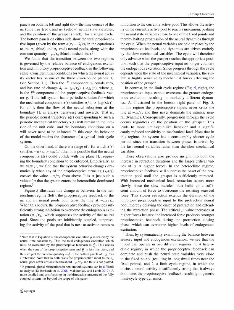
Fig. 5 A small change in endogenous excitation near the critical valueof μ switches the dynamical regime. Top panels The trajectories ofthe state variables over a single cycle, for μ values just below andabove the transition point, when Fsw = 0.05. The top left panelshows trajectories for the heteroclinic regime (μ1 = 1.6 × 10−5),whereas the top right panel shows trajectories for the limit cycle regime(μ2 = 1.8 × 10−5). In both plots, the a0 (protraction open), a1 (pro-traction closing) and a2 (retraction) variables are shown in blue, red,and yellow, respectively. The position of the grasper is plotted in black,with 1 corresponding to full protraction and 0 to full retraction. Thethick portion of the curve indicates where the grasper is closed. Thelimit cycle regime trajectory has a shorter cycle period relative to theheteroclinic regime trajectory (note 0.5 ms scale bars left and right),and this difference is primarily manifested in durations of the a0 and a2neural pools. Bottom panels The proprioceptive inputs to the a0 (blue)

and a1 (red) neural pools, for the heteroclinic regime (left), and thelimit cycle regime (right). The dashed black lines show the constantvalues −μ1/τa (left) and −μ2/τa (right) for reference. Note that in theheteroclinic regime example (left), the proprioceptive feedback curvescross the horizontal line at −μ1/τa. In this regime, sensory feedbackis able to overcome the neural dynamics and “pin” the neural statevariables to one of the fixed points until the appropriate mechanicalstate is reached. In contrast, in the limit cycle regime example (right),the proprioceptive feedback curves never cross the line at −μ2/τa. Inthis regime, the proprioceptive input never exceeds the intrinsic neuraldynamics and thus has only a weak effect on the cycle timing. Notethat in the heteroclinic regime (left) the grasper is able to retract morefully, which both increases the proprioceptive feedback and allows forgreater inward seaweed movement

J Comput Neurosci

panels on both the left and right show the time courses of thea0 (blue), a1 (red), and a2 (yellow) neural state variables,and the position of the grasper (black), for a single cycle.The bottom panels on either side show the total propriocep-tive input (given by the term ε(xr − Si)σi in the equations)to the a0 (blue) and a1 (red) neural pools, along with theconstant quantity −μ/τa (black, dashed line).2

We found that the transition between the two regimesis governed by the relative balance of endogenous excita-tion and inhibitory proprioceptive feedback, in the followingsense. Consider initial conditions for which the neural activ-ity vector lies on one of the three lower-bound planes �i

(see Section 3.1). Then the i th component ai equals zero,and has rate of change ai = (μ/τa) + εgi (x), where giis the i th component of the proprioceptive feedback vec-tor g. If the full system has a periodic solution for whichthe mechanical component x(t) satisfies μ/τa > |εg(x(t))|for all t , then the flow of the neural subsystem at theboundary �i is always transverse and inwards. That is,the periodic neural trajectory a(t) corresponding to such aperiodic mechanical trajectory x(t) will remain in the inte-rior of the unit cube, and the boundary conditions on awill never need to be enforced. In this case the behaviorof the model retains the character of a typical limit cyclesystem.

On the other hand, if there is a range of t for which x(t)satisfies −μ/τa > εgi(x), then it is possible that the neuralcomponents a(t) could collide with the plane �i , requir-ing the boundary conditions to be enforced. Empirically, aswe vary μ, we find that the system behavior changes dra-matically when any of the proprioceptive terms εgi(xr (t))

crosses the value −μ/τa from above. It is at just such avalue of μ that the system enters the heteroclinic-dominatedregime.3

Figure 5 illustrates this change in behavior. In the het-eroclinic regime (left), the proprioceptive feedback to thea0 and a1 neural pools both cross the line at −μ1/τa.When this occurs, the proprioceptive feedback provides suf-ficiently strong inhibition to overcome the endogenous exci-tation (μ1/τa), which suppresses the activity of that neuralpool. Since the pools are inhibitorily coupled, suppress-ing the activity of the pool that is next to activate removes

2Note that in Equation 4, the endogenous excitation μ is scaled by theneural time constant τa. Thus the total endogenous excitation whichmust be overcome by the proproceptive feedback is μ

τa. This occurs

when the sum of the proprioceptive term and μτa

is less than zero, and

thus we plot the constant quantity − μτa

in the bottom panels of Fig. 5 asa reference. Note that in both cases the proprioceptive input to the a2neural pool never crosses the threshold −μ/τa, and thus is not plotted.3In general, global bifurcations in non-smooth systems can be difficultto analyze (Di Bernardo et al. 2008; Makarenkov and Lamb 2012). Amore detailed analysis focusing on the bifurcation structure of the fullycoupled system lies beyond the scope of this paper.

inhibition to the currently active pool. This allows the activ-ity of the currently active pool to reach a maximum, pushingthe neural state variables close to one of the fixed points andthereby halting progression of the neural dynamics throughthe cycle. When the neural variables are held in place by theproprioceptive feedback, the dynamics are driven entirelyby the slow mechanical variables. The cycle will thereforeonly advance when the grasper reaches the appropriate posi-tion, such that the proprioceptive input no longer countersthe endogenous excitation. Since progress through the cycledepends upon the state of the mechanical variables, the sys-tem is highly sensitive to mechanical forces affecting theposition of the grasper.

In contrast, in the limit cycle regime (Fig. 5, right), theproprioceptive input cannot overcome the greater endoge-nous excitation, resulting in markedly different dynam-ics. As illustrated in the bottom right panel of Fig. 5,in this regime the proprioceptive inputs never cross theline at −μ/τa and thus never dominate the intrinsic neu-ral dynamics. Consequently, progression through the cycleoccurs regardless of the position of the grasper. Thisleads to more limit-cycle-like behavior and a signifi-cantly reduced sensitivity to mechanical load. Note that inthis regime, the system has a considerably shorter cycleperiod, since the transition between phases is driven bythe fast neural variables rather than the slow mechanicalvariables.

These observations also provide insight into both theincrease in retraction durations and the larger critical val-ues of μ at higher forces. In the heteroclinic regime,proprioceptive feedback will suppress the onset of the pro-traction pool until the grasper is sufficiently retracted.With increased mechanical load, retraction occurs moreslowly, since the slow muscles must build up a suffi-cient amount of force to overcome the resisting seaweedforce. This slower retraction extends the duration of theinhibitory proprioceptive input to the protraction neuralpool, thereby delaying the onset of protraction and extend-ing the retraction phase. The critical μ value increases athigher forces because the increased force produces strongerproprioceptive feedback during the protraction closingphase, which can overcome higher levels of endogenousexcitation.

Thus, by systematically examining the balance betweensensory input and endogenous excitation, we see that themodel can operate in two different regimes: 1. A hetero-clinic regime, in which the proprioceptive feedback candominate and push the neural state variables very closeto the fixed points (resulting in long dwell times near thefixed points), and 2. a limit cycle regime, in which theintrinsic neural activity is sufficiently strong that it alwaysdominates the proprioceptive feedback, resulting in genericlimit-cycle-type dynamics.

J Comput Neurosci

5.2 Comparing the performance of the limit cycle regimeto the heteroclinic regime

We have seen that the model can operate in one of two dis-tinct dynamical regimes, with the primary distinction beingthat in one regime (the heteroclinic regime), the neuraldynamics are sensitive to proprioceptive input and mechani-cal load, while in the other (the limit cycle regime), they arenot. Next we ask whether the enhanced sensitivity to loadseen in the heteroclinic regime confers any functional orbehavioral advantages. We therefore explore the efficacy ofthe limit cycle and heteroclinic regimes in the ingestion ofseaweed over a range of resisting forces on the seaweed. Asa representative example of a system falling within the het-eroclinic regime, we ran the model with the very small butnon-zeroμ value of 10−9. We do not set this parameter iden-tically equal to zero since for this (and only this) value theisolated neural dynamics possess a heteroclinic cycle ratherthan a stable heteroclinic channel. As an example of the sys-tem in the limit cycle regime, we ran the simulation for themuch larger μ value of 10−3. These choices ensure that thetwo examples will lie safely on either side of the transitionpoint across all of the parameter ranges we explore.

Although the heteroclinic regime model can be switchedto the limit cycle regime by increasing the intrinsicexcitability μ, as shown in Fig. 6 (top line: heteroclinicregime, μ = 10−9; bottom line: limit cycle regime,

0.00 0.02 0.04 0.06 0.08 0.10

−0

.10

−0

.05

0.0

00

.05

0.1

0

Force on seaweed ( Fsw )

Ave

ra

ge

se

aw

ee

d v

elo

city

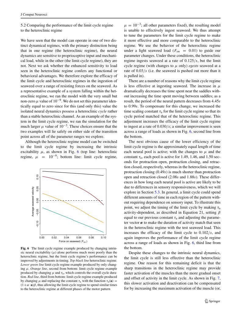
Fig. 6 The limit cycle regime example produced by changing intrin-sic neural excitability (μ) alone performs much more poorly than theheteroclinic regime, but the limit cycle regime’s performance can beimproved by adjustments in timing. Top black line heteroclinic regime.Lower green line limit cycle regime example produced by only chang-ing μ. Orange line, second from bottom: limit cycle regime exampleproduced by changing μ and τa, which controls the overall cycle dura-tion. Red line, third from bottom: limit cycle regime example producedby changing μ and replacing the constant τa with the function τa(a) =(1+α ·a)β, thus allowing the limit cycle regime to spend similar timesto the heteroclinic regime at different phases of the motor pattern

μ = 10−3; all other parameters fixed), the resulting modelis unable to effectively ingest seaweed. We thus attemptto tune the parameters for the limit cycle regime to makeit more effective and more comparable to the heteroclinicregime. We use the behavior of the heteroclinic regimeunder a light seaweed load (Fsw = 0.01) to guide ourparameter changes. Under these conditions, the heteroclinicregime ingests seaweed at a rate of 0.125/s, but the limitcycle regime (with changes to μ only) egests seaweed at arate of 0.03/s (i.e. the seaweed is pushed out more than itis pulled in).

There are a number of reasons why the limit cycle regimeis less effective at ingesting seaweed. The increase in μ

dramatically decreases the time spent near the saddles with-out increasing the time spent moving between saddles; as aresult, the period of the neural pattern decreases from 4.45sto 0.99s. To compensate for this change, we increased thetime scaling constant τa for the limit cycle regime so that itscycle period matched that of the heteroclinic regime. Thisadjustment increases the efficacy of the limit cycle regimeto ingest at a rate of 0.030/s; a similar improvement is seenacross a range of loads as shown in Fig. 6, second line fromthe bottom.

The next obvious cause of the lower efficiency of thelimit cycle regime is the approximately equal length of timeeach neural pool is active; with the changes to μ and theconstant τa, each pool is active for 1.49, 1.46, and 1.50 sec-onds for protraction open, protraction closing, and retrac-tion closed, respectively, whereas in the heteroclinic regime,protraction closing (0.49s) is much shorter than protractionopen and retraction closed (2.08s and 1.88s). These differ-ences in how long each neural pool is active are likely to bedue to differences in sensory responsiveness, which we willexplore in Section 5.3. In general, a limit cycle could spenddifferent amounts of time in each region of the pattern with-out requiring dependence on sensory input. To illustrate thispoint, we adjust the timing of the limit cycle by making τa

activity-dependent, as described in Equation 21, setting β

equal to our previous constant τa and adjusting the parame-ter vector α to make the duration of activity match that seenin the heteroclinic regime with the test seaweed load. Thisincreases the efficacy of the limit cycle to 0.102/s, andagain improves the performance of the limit cycle regimeacross a range of loads as shown in Fig. 6, third line fromthe bottom.

Despite these changes to the intrinsic neural dynamics,the limit cycle is still less effective than the heteroclinicregime. One reason for this remaining deficit is that thesharp transitions in the heteroclinic regime may providefaster activation of the muscles than the more gradual onsetand offset of activity in the limit cycle. As shown in Fig. 7,this slower activation and deactivation can be compensatedfor by increasing the maximum activation of the muscle (or,

J Comput Neurosci

0.00 0.02 0.04 0.06 0.08 0.10

0.0

00

.05

0.1

0

Force on seaweed ( Fsw )

Ave

rag

e s

eaw

ee

d v

elo

city

Fig. 7 Increasing the maximum muscle activation allows the systemin the limit cycle regime to perform as well as that in the heteroclinicregime, over a range of forces. Black line heteroclinic regime. Redline, yellow line, green line, and blue line: limit cycle regime withtiming changes and 1, 1.2, 1.4, or 1.6 times the maximum muscleactivation, respectively

equivalently, the cross section of the muscle) umax. Increas-ing umax by a factor of 1.6 results in a rate of ingestion of0.126, which is slightly higher than the efficacy of the hete-roclinic regime. Note that, as shown in the figure, even withhigher values of umax, the heteroclinic regime is more effec-tive than the limit cycle regime when the mechanical loaddue to the seaweed increases .

Although increasing the maximum muscle activationallows the limit cycle regime to match or even exceedthe efficacy of the heteroclinic regime over a range of

0.00 0.02 0.04 0.06 0.08 0.10

34

56

78

91

0

Force on seaweed ( Fsw )

Inte

gra

ted

mu

scle

activity p

er u

nit le

ng

th o

f se

aw

ee

d

Fig. 8 Increased muscle activation in the limit cycle regime comesat a metabolic cost (see Eq. (25)). Black line heteroclinic regime. Redline, yellow line, green line, and blue line: limit cycle regime withtiming changes and 1, 1.2, 1.4, or 1.6 times the maximum muscleactivation, respectively

loads, this change has a metabolic cost for the animal. Toa first approximation, the energetic cost of contraction isproportional to the force generated by the muscle (Saccoet al. 1994). Thus, under the model’s assumption that weare in the linear regime of the force-activation curve, theenergetic cost of contraction is also proportional to theactivation of the muscle. In Fig. 8 we show the energeticcost, in the form of integrated muscle activation over time,per length of seaweed ingested. Assuming the system hasreached steady-state, this is

∫ T

0

∑i ui(t) dt

xsw(0)− xsw(T ), (25)

where T is the period of the behavior. Note that even at lowloads, the limit cycle regime pays a higher metabolic costper unit length of seaweed ingested.

The behavior of the limit cycle regime is also mechani-cally less efficient at higher loads. In Fig. 9, we show themechanical work done by the muscles per unit length ofseaweed ingested,

∫ T

0 Fmusc(s)dxrdt

∣∣∣t=s

ds

xsw(0)− xsw(T ). (26)

Note that the limit cycle regime is able to remain mechani-cally efficient over a larger range of loads when the musclesare strengthened, but the heteroclinic regime is still moremechanically efficient at higher loads than the limit cycleregime with muscles that are 1.6 times stronger. We willexplore the differences in behavior that lead to these effectsin the next section.

0.00 0.02 0.04 0.06 0.08 0.10

0.2

50

.30

0.3

50

.40

0.4

50

.50

Force on seaweed ( Fsw )

Wo

rk d

on

e b

y m

uscle

s p

er u

nit le

ng

th o

f se

aw

ee

d

Fig. 9 With higher loads, the system in the limit cycle regime is lessefficient than in the heteroclinic regime, and does more mechanicalwork (Eq. (26)) for a given amount of seaweed ingested. Black lineheteroclinic regime. Red line, yellow line, green line, and blue line:limit cycle regime with timing changes and 1, 1.2, 1.4, or 1.6 times themaximum muscle activation, respectively

J Comput Neurosci

5.3 Mechanisms of adaptation to load

How do the two architectures adapt to changes in mechan-ical load? In Fig. 10, we can see the changes betweenlow and high seaweed forces. In the limit cycle regime,the time course of neural activation is very similar underboth high (Fsw = 0.1) and low (Fsw = 0.01) loadconditions. As a result, the forces in the high-load con-dition dramatically reduce the distance that the seaweed

is pulled inward before the grasper releases the seaweed(thick green line). Note that once the seaweed is released,the retraction force on the grasper is no longer opposed,causing a rapid retraction. In the heteroclinic regime, bycomparison, we can see that the neural pool involved inretraction (yellow) increases its duration of activity. Theresulting long retraction allows the animal to draw in moreseaweed by allowing the muscles to exert a greater peakforce.

Heteroclinic Regime Limit Cycle Regime

Low

mechanicalload

280 285 290 295 300

0.0

0.4

0.8

Time (s)

Po

sitio

n

280 285 290 295 300

0.0

0.4

0.8

Time (s)

Po

sitio

n

280 285 290 295 300

0.0

0.4

0.8

Time (s)

Activity

280 285 290 295 300

0.0

0.4

0.8

Time (s)

Activity

High

mechanicalload

280 285 290 295 300

0.0

0.4

0.8

Time (s)

Po

sitio

n

280 285 290 295 300

0.0

0.4

0.8

Time (s)

Po

sitio

n

280 285 290 295 300

0.0

0.4

0.8

Time (s)

Activity

280 285 290 295 300

0.0

0.4

0.8

Time (s)

Activity

Fig. 10 Forces on seaweed can selectively prolong the retractionphase of the heteroclinic regime, but have little effect on the limitcycle regime. Black and green lines show the position of the grasper,with the thick green sections showing the positions when the grasperis closed on the seaweed and the black sections showing the positionswhen the grasper is open. The blue, red and yellow lines show theactivity of the protraction open, protraction closing, and retractionclosed neural pools, respectively. The mechanical load, Fsw wasincreased from 0.01 to 0.1. The positions of the grasper are similar

for both the heteroclinic regime and the limit cycle regime whenthere is little load. Note that the duration of retraction closed (yellow)increases substantially in the heteroclinic regime under high load,resulting in a stronger retraction while holding the seaweed; this isnot true in the limit cycle regime under load. The sensitivity to load inthe heteroclinic regime is due to sensory feedback counteracting theendogenous excitation and delaying the onset of the protraction neuralpool, as demonstrated in Figs. 4 and 5

J Comput Neurosci

This difference in response is consistent with our obser-vations in Fig. 4 that, in the heteroclinic regime, the systemcompensates for higher loads by increasing the duration ofthe retraction neural pool activity, whereas in the (untuned)limit cycle regime, the system is largely insensitive to sea-weed forces. To examine more systematically how the tunedlimit cycle regime responds to changes in force, in Fig. 11we plotted the retraction neural pool duration across arange of forces for both the heteroclinic and limit cycleregime examples. Here we see clearly that the heteroclinicregime example systematically increases retraction dura-tion in response to increasing force, whereas the limit cycleregime example is insensitive to changes in load, even whenthe time constants and muscle activation parameters havebeen tuned.

The mechanisms of these changes in timing can be seenin more detail in Fig. 12. In both the heteroclinic and limitcycle regimes, the trajectory is moved only a small distanceby sensory input. In the case of the limit cycle regime, thenew trajectory passes through a very similar region of phasespace as the unperturbed trajectory, and thus the timing ofthe oscillation does not change very much. In contrast, inthe heteroclinic regime, the small perturbation moves thetrajectory near the saddle point where the flow decreasesrapidly even over these short distances. During retraction,the trajectory passes closer to the saddle where the flow isvery small; thus it spends longer in this region.

It is natural to ask whether the intact behaving animalemploys similar strategies. Because it is difficult in theintact animal to assess the dynamic forces generated byseaweed bunching up in the buccal cavity as seaweed is

0.00 0.02 0.04 0.06 0.08 0.10

2.0

2.2

2.4

2.6

Force on seaweed ( Fsw )

I3 n

eu

ra

l p

oo

l d

ura

tio

n (

s)

Heteroclinic regime

Limit cycle regime

Fig. 11 In the heteroclinic regime (black line, μ = 10−9), the systemreacts to increasing the seaweed force by lengthening the duration ofthe retraction neural pool activity. In contrast, retraction duration inthe limit cycle regime example (blue line, μ = 10−3) is relativelyinsensitive to mechanical load, despite adjustments to the neural timeconstants and the maximum muscle activation parameter

ingested, we consider a simplified situation where a stiffelastic force is encountered during a swallow that preventsthe seaweed from moving inward, such as the holdfast of theseaweed. We can create an analagous situation in the ani-mal by feeding the animal a thin strip of seaweed and thenholding the seaweed during a swallow to present a resistingforce.

How do these strategies compare to those used by theanimal itself? As shown in Fig. 13, when seaweed is held bythe experimenter to prevent inward movement, the durationof retraction increases, although the duration of protractiondoes not appear to increase or decrease.

It is not surprising that an animal would behave in anadaptive manner to the behaviorally relevant task of con-suming seaweed. If the dynamics of the central nervoussystem are heteroclinic regime-like, would this create anychanges that would not be expected from a purely adaptivestandpoint? There are two we will discuss here: the responseto removal of proprioceptive and excitatory input, and theshape of the distribution of durations of components of thepattern.

The removal of sensory input and excitatory drive canbe simulated by setting ε and μ equal to zero. For theseparameters, the system possesses a true heteroclinic cycle,and in the absence of noise or intrinsic excitability the dura-tion of patterns will grow without bound. In our preparationsof the isolated buccal ganglia, we observed that the iso-lated neural system did possess a small but not zero amountof intrinsic excitability. Therefore we simulated this situa-tion by setting μ equal to a very small but non-zero value(μ = 10−30). Note also that the addition of noise could alsoproduce oscillations in the pure heteroclinic cycle, leadingto long, but still finite, cycle times. In Fig. 14 (left), we setμ to 10−30 to show that even a very small amount of con-stant excitation is sufficient to prevent the heteroclinic cyclefrom becoming “stuck” in one of the phases. In this case wesee that the pattern duration is much longer than either theheteroclinic regime or limit cycle regime examples we havepreviously explored, which both have non-zero values of μ.Furthermore, this lengthening of the pattern is observed inall three motor components. It is important to note that thislengthening of the patterns depends upon the presence ofan underlying heteroclinic architecture, since the slowing ofthe neural trajectory occurs due to the passage of the trajec-tory near a series of fixed points. If we reduce the influenceof the fixed points by increasing μ, thereby making the sys-tem resemble a generic limit cycle (Fig. 14, right), thenthe removal of sensory input has very little effect (compareFig. 14 top right and bottom right).

When sensory input is removed from the animal, does theduration of protraction and retraction increase as is seen inthe heteroclinic regime, or remain about the same as is seenin the limit cycle regime? To investigate this, we examine

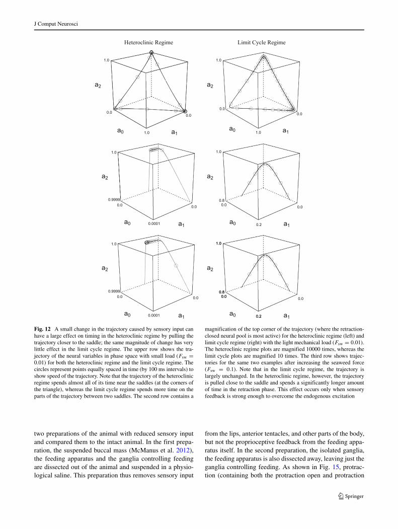
J Comput Neurosci

emigeRelcyCtimiLemigeRcinilcoreteH

0.0

1.0

1.0

0.0

a0

a2

1.0

0.0

1.0

a2

a0

a2

a1

0.9999

1.0

0.0

0.0001

0.0 0.00.8

1.0

0.0

0.2a0

a2

a1

0.9999

1.0

0.0

a0

a2

a10.0001

0.0 0.00.8

1.0

0.2a0

a2

a1

0.00.8

1.0

0.0

0.2

0.0

a0 a1a1

Fig. 12 A small change in the trajectory caused by sensory input canhave a large effect on timing in the heteroclinic regime by pulling thetrajectory closer to the saddle; the same magnitude of change has verylittle effect in the limit cycle regime. The upper row shows the tra-jectory of the neural variables in phase space with small load (Fsw =0.01) for both the heteroclinic regime and the limit cycle regime. Thecircles represent points equally spaced in time (by 100 ms intervals) toshow speed of the trajectory. Note that the trajectory of the heteroclinicregime spends almost all of its time near the saddles (at the corners ofthe triangle), whereas the limit cycle regime spends more time on theparts of the trajectory between two saddles. The second row contains a

magnification of the top corner of the trajectory (where the retraction-closed neural pool is most active) for the heteroclinic regime (left) andlimit cycle regime (right) with the light mechanical load (Fsw = 0.01).The heteroclinic regime plots are magnified 10000 times, whereas thelimit cycle plots are magnified 10 times. The third row shows trajec-tories for the same two examples after increasing the seaweed force(Fsw = 0.1). Note that in the limit cycle regime, the trajectory islargely unchanged. In the heteroclinic regime, however, the trajectoryis pulled close to the saddle and spends a significantly longer amountof time in the retraction phase. This effect occurs only when sensoryfeedback is strong enough to overcome the endogenous excitation

two preparations of the animal with reduced sensory inputand compared them to the intact animal. In the first prepa-ration, the suspended buccal mass (McManus et al. 2012),the feeding apparatus and the ganglia controlling feedingare dissected out of the animal and suspended in a physio-logical saline. This preparation thus removes sensory input

from the lips, anterior tentacles, and other parts of the body,but not the proprioceptive feedback from the feeding appa-ratus itself. In the second preparation, the isolated ganglia,the feeding apparatus is also dissected away, leaving just theganglia controlling feeding. As shown in Fig. 15, protrac-tion (containing both the protraction open and protraction

J Comput Neurosci

01

23

4

Dura

tion (

s)

+

+

+

++

+

+

+

+

+

+

+

+

+

++

+

++

+

+

++

+

+

+

+

+

+

+

+ +

+++

+

+

+

01

23

4

+

+++

+

+

++

+

+

+

+

+

+

+

+

+

+

+

+

+

+

+

+

+

+

+

+

+

+

+

+

+

+

+

+

+

+

not held

not held

held

held

Protraction Retraction

Fig. 13 When a force is applied to the seaweed in vivo (by holdingthe seaweed), the activity of the neurons involved in retraction (corre-sponding to retraction closed) is prolonged (right), while the activityof the protractor muscle (corresponding to the start of protraction opento the end of protraction closing) is not (left). Medians differ (Mann–Whitney test, p = 0.013). 30 unheld swallows and 7 held swallowswere used from the same two animals. Results are similar if unheldswallows from all 6 animals are used (not shown, p = 0.003)

closing phases) and retraction (closed) both increase induration from the intact animal to the suspended buccalmass, and increase further in duration from the suspendedbuccal mass to the fictive patterns of the isolated ganglia.Note that this increase in both protraction and retractiondiffers from the selective increase in retraction when theseaweed was held in Fig. 13, but matches the increasein both phases seen in the stable heteroclinic channel(Fig. 14).

When subject to small amounts of noise, the heteroclinicregime and the limit cycle regime show different forms ofvariability in timing. We illustrated this by running 10000independent stochastic simulations of the model with lowamplitude Gaussian noise (standard deviation η = 10−4),for both the heteroclinic regime model and the limit cycleregime model. The retraction neuronal pool durations werecollected from all simulations in both cases, and for eachcase we computed a distribution of duration times. Thedensity functions were estimated using a kernel densityestimator algorithm described in Silverman (1986). Eachdata point was convolved with a Gaussian kernel, and theresulting smoothed curves were summed to form a singlefunction. This function was then normalized by dividingby the total area under the curve. The kernel bandwidth ineach case was chosen based on the variance of the data(Silverman 1986).

The key result of simulations with noise, shown inFig. 16, is that the distribution for the heteroclinic regimeis significantly skewed compared to the more symmet-ric distribution for the limit cycle regime. In the limit

cycle regime, perturbations from the noise have very simi-lar effects regardless of where they occur in the cycle, so, bythe central limit theorem, their cumulative effect is approx-imately Gaussian in the limit of small noise.4 In contrast, inthe heteroclinic regime, as described in Shaw et al. (2012),perturbations that occur while approaching the saddle canhave much larger effects than perturbations that occur whileleaving the saddle, so the central limit theorem does notapply. As predicted by Stone and Holmes (1990), this resultsin a distribution that is skewed to the right.

Using our in vivo preparation, we can measure the retrac-tion duration during swallowing in intact Aplysia, and com-pare the resulting distribution to our simulation output. InFig. 17, we see that the distribution of retraction durationsis significantly skewed to the right, more closely resem-bling that seen in the heteroclinic regime of the model.The experimental distribution was computed via the samekernel density estimation procedure used for the simulateddata.

6 Discussion

In this paper, we have examined a neuromechanical modelof swallowing in Aplysia in two parameter regimes. In thefirst parameter regime, the internal neural dynamics drivethe cycle in a manner similar to an idealized central pat-tern generator. In contrast, in the second parameter regime,which has dynamics more similar to those of a chain reflex,passage near saddle points leads to greater sensitivity tosensory inputs.

We have shown that the model operating within the limitcycle regime does not adapt as well to changing loads as themodel operating within the heteroclinic regime, even whenthe durations of the cycle components have been tuned to bethe same in both regimes (Figs. 6–9). We showed that partof this change is due to a prolongation of retraction allowinggreater activation of the slow retractor muscles (Figs. 10,11). We then showed that the animal itself appears to usethe same strategy of prolonging retraction when faced withloads in vivo (Fig. 13).

We showed that, in the heteroclinic regime, the modelcould more accurately capture behaviors observed in exper-imental data than in the limit cycle regime, even foraspects of the behavior that do not convey an obviousevolutionary advantage. First, removal of sensory feed-back and reduction of endogenous excitation resulted in

4In the limit cycle regime, the time spent passing through one part ofthe cycle can be approximated as the first passage time of a Brown-ian particle with drift, so the small noise assumption is important; thedistribution will become skewed as the noise becomes large relative tothe drift.

J Comput Neurosci

emigeRelcyCtimiLemigeRcinilcoreteH

With

sensory

feedback

280 285 290 295 300

0.0

0.4

0.8

Time (s)

Positio

n

280 285 290 295 300

0.0

0.4

0.8

Time (s)

Positio

n

280 285 290 295 300

0.0

0.4

0.8

Time (s)

Activity

280 285 290 295 300

0.0

0.4

0.8

Time (s)

Activity

Without

sensory

feedback

280 285 290 295 300

0.0

0.4

0.8

Time (s)

Positio

n

280 285 290 295 300

0.0

0.4

0.8

Time (s)

Positio

n

280 285 290 295 300

0.0

0.4

0.8

Time (s)

Activity

280 285 290 295 300

0.0

0.4

0.8

Time (s)

Activity

Fig. 14 Removing sensory feedback and endogenous excitation bysetting ε = 0 and μ = 10−30 slows both protraction and retractiondue to the underlying heteroclinic cycle architecture. For reference,the top two panels on the left and right show example trajectories forthe heteroclinic and limit cycle regimes, respectively (identical to thetop panels of Fig. 10). The two panels at bottom left show example

trajectories resulting from the removal of sensory input and endoge-nous excitation (ε = 0 and μ = 10−30). When the system is made toa resemble a standard limit cycle by setting μ = 10−3, the removalof sensory input no longer has an effect, as seen in the two panels atbottom right

slowed cycling in the model (Fig. 14, left), due to theunderlying stable heteroclinic channel architecture. In themodel, however, when the endogenous excitation of theneurons was increased so that the neural dynamics enteredthe limit cycle regime, the removal of sensory input hadessentially no effect on the model’s dynamics (Fig. 14,right). Interestingly, slowed cycling was also observedexperimentally in the animal when sensory inputs to thebuccal ganglia were removed (Fig. 15). This is consis-tent with the model in the heteroclinic regime but notthe limit cycle regime. Second, the distribution of burst

durations in the model showed a very skewed distri-bution in the heteroclinic regime but not in the limitcycle regime (Fig. 16). A similarly skewed distribution ofretraction durations was observed experimentally in vivo(Fig. 17).

6.1 Limitations of the model and results

We have intentionally created a very nominal model ofswallowing behavior which does not capture many of thedetails known about feeding in Aplysia. As previous work

J Comput Neurosci

05

10

15

Dura

tion

(s)

+

+

+

+

+

+

++

+

+

+

+

+

+++

+

+++

+++++++++++++++

++

++

+

+++++++++++

++

+

++

+

+

+

+++

++

++

+++

+

++

+

++

+

+

++

+

+

+

+

+

+++

+++

+

+

++

++

+++++++++

+

+

++

+

+

++

+

+

+

+

+

++

+

+

+++++

+

++

+

++

+

+++

++

+

+

+

+

+

++++

++

+

+

+

+

+

+

++

+

+

+

+

+

+

++

+

05

10

15

++

+

+++

+

++++

+

+

+++

++++

+

++++++

+++

+

+

+

+

+

++

+

+

+++++++

+

++++++++++++++

++++++

+

++++

++

++

++++++++++++++

+++++++

+

++++++

+++

++++++++

++

+

++

++

+

+

+++++

+

++++

+++++

+++++

++

++++++

++

+

++++++

+

+

+++

+

in viv

o

in viv

o

SB

M

SB

M

ganglia

ganglia

Protraction Retraction

Fig. 15 Protraction and retraction intervals are longer in the sus-pended buccal mass than in the intact animal, and longer in the isolatedganglia than in either the suspended buccal mass or the intact animal.Bites were used (rather than swallows) because there is no clear ana-log of a swallow in the isolated ganglia. Medians differ significantlyby preparation type for both protraction (Kruskal–Wallis, p < 0.001)and retraction (Kruskal–Wallis, p < 0.001). Results are similar whenswallows from the in vivo and suspended buccal mass preparationsare used instead of bites (not shown, p < 0.001 for both protractionand retraction). Recordings in vivo: 146 bites from 6 animals. Sus-pended buccal mass: 8 bites from 2 animals. Isolated ganglia: 13 motorpatterns from 2 animals

0.6 0.8 1.0 1.2 1.4

01

23

45

Heteroclinic regime retraction duration (s)

De

nsity

1.82 1.83 1.84 1.85

02

04

060

80

Limit cycle regime retraction duration (s)

De

nsity

Fig. 16 In the presence of small amounts of noise, retractions are sig-nificantly more skewed for the heteroclinic regime than for the limitcycle regime (skewness = 0.91 vs 0.03, for the heteroclinic regimeand limit cycle regime respectively. D’Agostino test for skewness(D’Agostino et al. 1990):

√b1 = 32 vs 1.1, p < 0.001 vs p = 0.27).

Shown is the kernel density estimator for the last a2 duration in eachof 10000 simulations with noise magnitude η = 10−4. Kernel den-sity estimation was performed using the algorithm given in Silverman(1986), which involves convolving the data with a Gaussian kernel anddividing by the total area of the resulting function. Kernel width waschosen based on the variance of the data (Silverman 1986)

−1 0 1 2 3 4 5 6

0.0

0.1

0.2

0.3

0.4

0.5

0.6

Retraction duration (s)

De

nsity

Fig. 17 Retraction durations are significantly skewed during swallow-ing patterns in intact Aplysia californica (skewness = 1.4, D’Agostinotest for skewness (D’Agostino et al. 1990):

√b1 = 4.56, p < 0.001).

Shown is the kernel density estimator (see the caption to Figure 16 fora description of the algorithm) of the total duration of B6/B9 and B3activity from 84 swallowing patterns in 6 animals

from our lab and others has shown, there are many degreesof biomechanical freedom beyond protraction and retrac-tion that influence the efficacy of feeding (Sutton et al.2004a, b; Novakovic et al. 2006), the muscles involvedhave many properties which we do not include in ourmodel (Yu et al. 1999; Zajac 1989), and the mechanics ofseaweed are much more complex than we have representedin the model (Denny and Gaylord 2002; Harder et al. 2006).Similarly, the dynamics of proprioception are much morecomplex than the linear model we have used (Evans andCropper 1998), and there are more than three pools of neu-rons involved in feeding behavior (Hurwitz et al. 1997),with dynamics that are much more complex than the firingrate model we have used (Susswein et al. 2002). In addi-tion, neuromodulation and learning may alter the dynamicsof the network slowly over time (Nargeot and Simmers2012; Susswein and Chiel 2012). Thus we expect at best aqualitative match to the in vivo behavior, and cannot com-pare the results against other models as rigorously as couldbe done with a model capable of quantitative predictions.

A nominal model may also have advantages. As com-plexity is added to a model, it can become more difficultto interpret the mechanics and, as a result, less clear whatdetails of the dynamics are responsible for an observedaspect of the behavior. In addition, as the parameter spacegrows, it becomes less obvious how dependent the resultsare on the particular choice of parameters (Foster et al.1993). Thus the nominal model we have used makes it clearthat passage near a saddle point results in enhanced sensitiv-ity to sensory perturbations, and the role of the parameters increating these dynamics can be easily understood in an intu-itive manner. In addition, the dynamics we have included

J Comput Neurosci

in the model, (e.g. mutually inhibitory neural pools, slowantagonistic muscles, and a slow muscle transfer function)are common to many other systems. Thus the qualitativebehavior of the model can be more readily generalized to avariety of other systems, which would be more difficult witha highly detailed model.

It is possible that some omitted details are criticalfor representing the behavior of the actual system. Forexample, intense bursting in the neural pools involves oscil-lations in fast variables such as membrane potential andsome gating variables. In our model these bursts are rep-resented in terms of passage near a saddle, where the statevariables are changing slowly. Many neuronal systems,however, can be decomposed into fast and slow subsystems(Butera et al. 1996; Krupa et al. 2008; Sherwood andGuckenheimer 2010), and slow passages near saddles mayoccur in the dynamics of the slow state variables, asdescribed by Nowotny and Rabinovich (2007). Ideally, onewould want to create a more detailed model of feedingin Aplysia and then use a principled reduction to find theslower dynamics. The work done in this paper may beuseful for guiding such a reduction.

One should also note that certain features of the exper-imental data that are well fit by our model based on astable heteroclinic channel architecture may also be com-patible with other dynamical architectures. For example, theskewed distribution of burst durations seen in the hetero-clinic regime (Fig. 16) could also be produced by a systemin which transitions between a series of stable equilibriaare induced by noise. Indeed, attractor networks have beenused as models for motor pattern generation (Cruse et al.1998), and it may be possible to model Aplysia feedingusing such a system. Further work would need to be done tocharacterize the respective roles of proprioceptive feedbackand endogenous excitation in such systems and to com-pare them with experimental data. However, the goal of thepresent work is not to rule out all other possible dynami-cal architectures consistent with experimental observations.Rather, our emphasis is on proposing the heteroclinic chan-nel architecture as an empirically motivated alternative tothe traditional limit cycle formulation of central patterngenerators.

6.2 Larger implications for pattern generators

6.2.1 Biological aspects

Many previous authors have noted the difference betweenpatterns seen in vitro and those seen in vivo, but the fieldhas not yet reached a consensus about the source of thesedifferences. In this paper, we propose that passage of trajec-tories near a fixed point provides a model that can explainsome of the distortions in timing seen in vitro. Furthermore,

this dynamical structure may help a pattern generator bet-ter use sensory input to adapt to a changing environment,and thus this structure may be selected for by evolutionarypressures. Although stable heteroclinic cycles are not struc-turally stable and thus are unlikely to be seen in a biologicalcontext, stable heteroclinic channels are structurally stableand robust to parameter variations and noise (Afraimovichet al. 2004b), and thus they are plausible dynamics for abiological system. The passage near fixed points as a wayof controlling timing has been seen in other models, forexample (Spardy et al. 2011c).

Many other pattern generators that have been previouslyidentified may lie between the two extremes on this con-tinuum between ideal central pattern generators and chainreflexes. Slower patterns in the absence of innervation havebeen seen in lamprey swimming (Wallen and Williams1984), crayfish walking (Chrachri and Clarac 1990), andlocust flight (Pearson et al. 1983).

These models of pattern generation may also be rele-vant in clinical contexts. In mammals, fictive respiration canbe observed in the isolated central nervous system and ishypothesized to arise from the interaction of two patterngenerators in the medulla – an inspiratory pattern generatorin the pre-Botzinger complex and an expiratory pattern gen-erator in the retrotrapezoidal-parafacial area (Tomori et al.2010). It has been known for some time, however, thatvagotomy (cutting the vagus nerve, which contains sensoryafferents involved in respiration) causes a dramatic slowing,but not cessation, of respiration. Qualitatively, this behavioris much closer to what we have shown in the stable hete-roclinic channel model, and not that of an idealized limitcycle. This would suggest that small perturbations may beenough to cause the changes seen in central sleep apnea andpossibly sudden infant death syndrome, but also suggeststhat the system may remain quite sensitive to certain pertur-bations even in the pathological state. In the case of centralsleep apnea, good models of the dynamics and sensitivity tosensory input might allow for new treatment modalities suchas transcranial direct current stimulation during episodes ofapnea or hypopnea.

6.2.2 Mathematical implications

Many of the behaviors we have observed in the stableheteroclinic channel regime may depend primarily on local-ized regions of the dynamics where the intrinsic dynam-ics, f (a, μ), are smaller than the proprioceptive feedback,εg(a, x). When the intrinsic excitability μ is sufficientlystrong that f (a, μ) > |εg(a, x)| for all values of a and x, thesensory input will have little effect on the temporal dynam-ics of the neural system. In this second regime, the neuraldynamics are largely insensitive to changes in mechanicalload or perturbations.

J Comput Neurosci

Although we have used a stable heteroclinic channel inour model to create localized regions of slowing, severalrelated dynamical architectures may produce similar effects.For example, in a saddle-node bifurcation on an invariantcycle, the flow around a limit cycle slows near a point asone approaches the bifurcation. This slowing may createqualitatively similar behavior.5 Other examples may includerelaxation oscillators where some parts of the trajectory aremuch slower than others, e.g. a Van der Pol oscillator (vander Pol 1926), which can create similar regions of sensitiv-ity (Bassler 1986) that may be relevant for motor patterngeneration (Rowat and Selverston 1993; Nadim et al. 2011).Half-center oscillator systems can also exhibit localizedslowing, which can affect the response of pattern generatorsto sensory input (Zhang and Lewis 2013; Daun et al. 2009;Daun-Gruhn 2011; Skinner et al. 1994).

Localized regions of slowing may not always be apparentin a model as it is written. For example, many dynami-cal models, such as bursting cells, may not have localizedregions of slowing in the form that they are written, but canbe decomposed using fast-slow analysis into state variablesthat change on different time scales. In these systems, sad-dle points may exist in the slower state variables that werenot apparent in the complete system.

The Equilibrium Point Hypothesis (EPH) states thatmotor trajectories could be understood as the result of a con-trol process that sets up one or a sequence of biomechanicalequilibrium points (Feldman 1966). Typically, the control isset by an unspecified central mechanism that may take intoaccount high-level sensory (visual, auditory) or goal-relatedinformation. Our framework is consistent with the EPH.When the system (1–2) has ε set to zero, the autonomouscentral dynamics has a fixed point atg for which the targetconfiguration, xtg, is a fixed point of the biomechanics, i.e.h(atg, xtg) = 0, with a suitable adjustment in the case of anonzero load. The incorporation of sensory feedback fromthe motor apparatus in the EPH is implicit in the setting ofthe neural equilibrium point.

Recent investigations have explored both experimentaland theoretical approaches to understanding how oscilla-tory pattern generators incorporate sensory feedback. Daun-Gruhn and Buschges emphasize these issues in modelingapproaches to understanding control of stepping motions ininsects. As they point out, successful walking on irregular

5The similarity actually goes deeper than this; if one adds a new statevariable representing the bifurcation parameter μ and sets dμ/dt = 0,the limit cycle in the augmented system now passes near a degeneratesaddle at μ = 0.

terrain requires coordinated activation of multiple musclegroups within each limb, as well as coordination betweenlimbs. In the stick insect system, it has been shown thatsensory feedback carries information both about joint posi-tion and about external loads, and that this feedback impactsboth the timing and intensity of motor neuron activation(Buschges and Gruhn 2007; Daun-Gruhn and Buschges2011). Furthermore, Daun-Gruhn and colleagues discusshow changing a single parameter representing endogenousexcitation can cause a half-center oscillator system to tran-sition from a stable limit cycle regime to a regime in whichinitiation of each phase of the oscillation is contingent on atransient sensory input signal, analogous to a discontinuousbistable chain reflex model (Daun et al. 2009; Daun-Gruhn2011). In addition, Paoletti and Mahadevan have recentlyproposed a model for the coordination of peristaltic contrac-tions underlying crawling motility in soft bodied organisms.In their model, coordination of central neural activationbetween adjacent body segments is mediated not by synap-tic connections, but by mechanical interactions affectingthe neural elements via sensory feedback through stretchreceptors (Paoletti and Mahadevan 2014).

Understanding how sensitivity to perturbations differs inthe heteroclinic and limit cycle regimes may also proveuseful as a diagnostic tool for probing the intrinsic dynam-ics of the pattern generating circuit. It has been shown inother cases that phase response curves can provide usefulinsights into the underlying dynamics of oscillatory pat-tern generators. For example, Zhang and Lewis (2013) haveshown that the phase response curves of half-center oscil-lator (HCO) circuits can be used to determine whetherprogression through the cycle is governed by an “escape”or a “release” type mechanism (Wang and Rinzel 1992).They found that in the escape-dominated regime, the systemwas sensitive to perturbations to the inactive cell as it wasbecoming active, whereas in the release-dominated regimethe opposite was true. Furthermore, they demonstrated thatthe sensitivity of their system to external inputs resultedfrom the presence of fixed points near the limit cycle inphase space, which is analogous to what we have observedin our heteroclinic channel model. It remains to be seenwhether the oscillations in our model are governed primarilyby release or escape and how this depends upon the balanceof endogenous excitation and proprioceptive feedback. Itmay also be useful to compare the phase response curves ofthe uncoupled neural system to those obtained when propri-oceptive feedback is present. As we have shown elsewhere,one can analyze the infinitesimal phase response curve foran uncoupled heteroclinic channel model (Shaw et al. 2012).

Acknowledgments This work was partially supported by bythe National Science Foundation (grants DMS-1010434 and IIS-1065489), the National Institute of Neurological Disorders and Stroke

J Comput Neurosci

(grant NS047073), the Simons Foundation (grant 259837 to PeterThomas), by the Council for the International Exchange of Scholars(CIES), and by sabbatical support from Case Western Reserve Univer-sity. Jeffrey Gill was supported by the Graduate Assistance in Areas ofNational Need program (P200A090191-11), Kendrick Shaw was par-tially supported by NIH grant T32-GM00725 and David Lyttle wassupported by an NSF Postdoctoral Fellowship (grant 1309380).

We are also grateful for helpful discussions with A. Horchler,A. Buschges and S. Daun-Gruhn, and for the comments of twoanonymous reviewers on an earlier version of the manuscript.

Conflict of interests The authors declare that they have no conflictof interest.

Appendix A Mathematical framework

Here we present the full model equations for the reader’sconvenience, and spell out how our model fits within thegeneral framework presented in Section 2. In this frame-work, the coupled neuromechanical system is written in theform:

dadt

= f (a, μ)+ εg(a, x), (27)

dxdt

= h(a, x)+ ζ l(x). (28)

In the specific example studied here, the vector a of neu-ral variables consists of a0, a1, and a2. The full equationsfor the neural state variables ai (noiseless case) are:

da0

dt= 1

τa(a0(1 − a0 − γ a1)+ μ)+ ε(xr − S0)σ0, (29)

da1

dt= 1

τa(a1(1 − a1 − γ a2)+ μ)+ ε(xr − S1)σ1, (30)

da2

dt= 1

τa(a2(1 − a2 − γ a0)+ μ)+ ε(xr − S2)σ2. (31)

These equations apply when ai ∈ (0, 1). At the bound-aries, strict rectifying boundary conditions are imposedwhich prevent ai from being greater than 1 or less than0. Specifically, when a neural variable is at 0, any furtherinhibitory input has no effect. Similarly, when a variable isat 1, any additional excitatory input has no effect. In thestochastic form of the equations each equation is amendedto include a ηdWi term.

Relating Eqs. (29–31) to Eq. (27) is straightforward. Here

fi(a, μ) = 1

τa(ai(1 − ai − γ ai+1)+ μ), (32)

and

εgi(a, x) = ε(xr − Si)σi . (33)

The vector of mechanical state variables x consists of u0,u1, xr and a binary variable ψ which takes the value of 0 or

1 depending on whether the grasper is open or closed. Theequations for the muscle activation variables ui are:

du0

dt= 1

τm((a0 + a1)umax − u0), (34)

du1

dt= 1

τm(a2umax − u1). (35)

Note that u0 activates the I2 muscle (protraction) andu1 activates the I3 muscle (retraction). The grasper can beeither open or closed. When a1 + a2 > 0.5, it is closed(ψ = 0), otherwise it is open (ψ = 1).

The position of the grasper (xr) is governed by theequation

dxr

dt= Fmusc

br(36)

when the grasper is open, and

dxr

dt= Fmusc + Fsw

br + bsw(37)

when it is closed.This can be written in terms of a singleequation as

dxr

dt= Fmusc

br + ψbsw+ ψ

Fsw

br + bsw. (38)

The grasper position is also subject to the rectifyingboundary conditions that prevent it from going above 1 orbelow 0.

The muscle force Fmusc is the sum of the I2 and I3muscles, given by

Fmusc =∑

i

kiφ

(xr − ci

wi

)

ui (39)

where φ(x) = −κx(x − 1)(x + 1) is the length-tensioncurve of the muscles (with κ = 3

√3/2), and i = 0, 1

denote the I2 and I3 muscles, respectively. Here xr ∈ [0, 1]is the position of the grasper, ki is a parameter representingthe strength and direction of each muscle, ci the position ofthe grasper where the ith muscle is at its minimum effec-tive length, and wi the difference between the maximumand minimum effective lengths for the ith muscle. The signof ki determines the direction of force of the muscle; whenki is negative (as it is for I2) the muscle will shorten as itmove the grasper forward toward the anterior portion of thejaws (protraction), and when it is positive (as it is for I3)it will shorten as it moves the grasper backward toward theposterior portion of the jaws (retraction).

Relating Eqs. (34–39) to Eq. (28), one can see that h(a, x)includes the equations governing the ui variables, the switchdetermining the open/closed state of the grasper, as wellas the equation governing xr. The term ζ l(x) refers to theapplied load, which is ψFsw/(br + bsw).

J Comput Neurosci

Appendix B Derivation of simplified biomechanics

The seaweed and grasper are assigned viscous damping con-stants bsw and br, respectively; thus the full equations ofmotion are

dxr

dt= vr, (40)

dxsw

dt= 0, (41)

dvr

dt= Fmusc − brvr

mr, (42)

dvsw

dt= 0 (43)

when the grasper is open, and

dxr

dt= dxsw

dt= vr, (44)

dvr

dt= Fmusc + Fsw − (br + bsw)vr

mr +msw, (45)

vsw = vr (46)

when the grasper is closed. Note that that we are assumingthat the momentum of the seaweed is negligible and that theseaweed is stationary when the grasper is open.

Table 1 Model parameters

Parameter Value Description

γ 2.4 inhibition strength from next poolε 0.002 sensory feedback strengthκ 3

√3/2 length-tension curve normalization constant

μ 10−9 neural pool intrinsic excitationτa 0.05 neural pool time constantτm 2.45 muscle activation time constantbr 0.1 grasper damping constantbsw 0.3 seaweed damping constantc0 1.0 position of shortest length for I2c1 1.1 position of center of I3Fsw 0.01 force on the seaweed resisting ingestionk0 −1 I2 muscle strength and directionk1 1 I3 muscle strength and directionσ0 −1 sign of proproceptive input to a0 neural poolσ1 1 sign of proproceptive input to a1 neural poolσ2 1 sign of proproceptive input to a2 neural poolS0 0.5 proprioceptive neutral position for protraction

open neural poolS1 0.5 proprioceptive neutral position for protraction

closing neural poolS2 0.25 proprioceptive neutral position for retraction

closed neural poolumax 1.0 maximum muscle activationw0 2 maximal effective length of I2w1 1.1 maximal effective length of I3

Table 2 State variables

State Initial Description

variable value

a0 1 − 10−9 activity of protraction open neural pool(non-negative)

a1 10−9 activity of protraction closing neural pool(non-negative)

a2 10−9 activity of retraction closed neural pool(non-negative)

u0 0 activity of I2 muscleu1 0 activity of I3 musclexr 0.5 grasper position (0 is retracted, 1 is

protracted)xsw 0 seaweed position (positive is away

from the animal)

Under the assumption that the system is criticallydamped, we can then use the following reduced system:dxr

dt= Fmusc

br, (47)

dxsw

dt= 0 (48)

when the grasper is open, and

dxsw

dt= dxr

dt= Fmusc + Fsw

br + bsw(49)

when the grasper is closed.

Appendix C Parameters and state variables

The meaning and default values of all the parameters (forthe heteroclinic regime) are given in the following table:

In the limit cycle regime, the neural time constant isrescaled by replacing the neural time constant τa with thefollowing activity-dependent time scaling function:

τa(a) = (1 + α · a)β (50)

where β is a uniform adjustment in the speed of the trajec-tories (analogous to the previous constant), and α is a vectorparameter representing an activity-dependent scaling of the

Table 3 Parameters used for the limit cycle simulations

Parameter Value Description

β 0.2262 neural pool global time constantμ 10−3 neural pool intrinsic excitationα0 0.59 neural pool local time scaling near

protraction openα1 −0.975 neural pool local time scaling near

protraction closingα2 0.32 neural pool local time scaling near

retraction closedumax 1.6 maximum muscle activation

J Comput Neurosci

speed. μ and umax are also altered. The values used in thelimit cycle regime are given in Table 3.

References

Afraimovich, V., Young, T., Muezzinoglu, M.K., Rabinovich, M.I.(2011). Nonlinear dynamics of emotion-cognition interaction:When emotion does not destroy cognition? Bulletin of Mathemat-ical Biology, 73(2), 266–284. doi:10.1007/s11538-010-9572-x.

Afraimovich, V.S., Rabinovich, M.I., Varona, P. (2004a). Heterocliniccontours in neural ensembles and the winnerless competition prin-ciple. International Journal of Bifurcation and Chaos, 14(04),1195–1208. doi:10.1142/S0218127404009806.

Afraimovich, V.S., Zhigulin, V.P., Rabinovich, M.I. (2004b). On theorigin of reproducible sequential activity in neural circuits. Chaos:An Interdisciplinary Journal of Nonlinear Science, 14(4), 1123.doi:10.1063/1.1819625. http://link.aip.org/link/CHAOEH/v14/i4/p1123/s1&Agg=doi.

Armbruster, D., Stone, E., Kirk, V. (2003). Noisy heteroclinic net-works. Chaos: An Interdisciplinary Journal of Nonlinear Science,13(1), 71–79.

Ashwin, P., Karabacak, O., Nowotny, T. (2011). Criteria for robust-ness of heteroclinic cycles in neural microcircuits. The Journal ofMathematical Neuroscience (JMN), 1(1), 1–18.

Bakhtin, Y. (2011). Noisy heteroclinic networks. Probability The-ory and Related Fields, 150(1–2), 1–42. doi: 10.1007/s00440-010-0264-0.

Baxter, D.A., & Byrne, J.H. (2006). Feeding behavior of Aplysia:A model system for comparing cellular mechanisms of clas-sical and operant conditioning. Learn Mem, 13(6), 669–680.doi:10.1101/lm.339206.

Bassler, U. (1986). On the definition of central pattern generatorand its sensory control. Biological Cybernetics, 54(1), 65–69.doi:10.1007/BF00337116.

Buschges, A., & Gruhn, M. (2007). Mechanosensory feedback inwalking: From joint control to locomotor patterns. Advances inInsect Physiology, 34, 193–230.

Butera, R.J., Clark, J.W., Byrne, J.H., Rinzel, J. (1996). Dissectionand reduction of a modeled bursting neuron. Journal of Compu-tational Neuroscience, 3(3), 199–223. doi:10.1007/BF00161132.http://www.springerlink.com/content/n2733052qjgj5761/.

Cataldo, E., Byrne, J., Baxter, D. (2006). Computational model of acentral pattern generator. In Computational methods in systemsbiology, lecture notes in computer science (Vol. 4210, pp. 242–256). Berlin / Heidelberg: Springer. doi: 10.1007/11885191 17.

Chrachri, A., & Clarac, F. (1990). Fictive locomotion in the fourth tho-racic ganglion of the crayfish, Procambarus clarkii. The Journal ofNeuroscience, 10(3), 707–719. http://www.jneurosci.org/content/10/3/707.

Church, P.J., & Lloyd, P.E. (1994). Activity of multiple identifiedmotor neurons recorded intracellularly during evoked feeding-like motor programs in Aplysia. Journal of Neurophysiology,72(4), 1794–1809. http://jn.physiology.org/cgi/content/abstract/72/4/1794.

Cruse, H., Kindermann, T., Schumm, M., Dean, J., Schmitz, J. (1998).Walknet—a biologically inspired network to control six-leggedwalking. Neural Networks, 11(7), 1435–1447.

Cullins, M.J., & Chiel, H.J. (2010). Electrode fabrication and implan-tation in Aplysia californica for multi-channel neural and muscularrecordings in intact, freely behaving animals. Journal of VisualizedExperiments, (40), doi:10.3791/1791.

D’Agostino, R.B., Belanger, A., D’Agostino, R.B. (1990). A sugges-tion for using powerful and informative tests of normality. TheAmerican Statistician, 44(4), 316–321. doi:10.2307/2684359.

Daun, S., Rubin, J.E., Rybak, I.A. (2009). Control of oscillation peri-ods and phase durations in half-center central pattern generators:A comparative mechanistic analysis. Journal of ComputationalNeuroscience, 27(1), 3–36.

Daun-Gruhn, S. (2011). A mathematical modeling study of inter-segmental coordination during stick insect walking. Journal ofComputational Neuroscience, 30(2), 255–278.

Daun-Gruhn, S., & Buschges, A. (2011). From neuron to behav-ior: Dynamic equation-based prediction of biological processes inmotor control. Biological Cybernetics, 105(1), 71–88.

Denny, M., & Gaylord, B. (2002). The mechanics of wave-sweptalgae. Journal of Experimental Biology, 205(10), 1355–1362.http://jeb.biologists.org/content/205/10/1355.

Di Bernardo, M., Budd, C.J., Champneys, A.R., Kowalczyk, P.,Nordmark, A.B., Tost, G.O., Piiroinen, P.T. (2008). Bifurca-tions in nonsmooth dynamical systems. Siam Review, 629–701.

Evans, C.G., & Cropper, E.C. (1998). Proprioceptive input to feed-ing motor programs in Aplysia. Journal of Neuroscience, 18(19),8016–8031. http://www.jneurosci.org/cgi/content/abstract/18/19/8016.

Feldman, A.G. (1966). Functional tuning of the nervous system withcontrol of movement or maintenance of a steady posture. II.Controllable parameters of the muscle. Biophysics, 11(3), 565–578.

Forssberg, H. (1979). Stumbling corrective reaction: A phase-dependent compensatory reaction during locomotion. Journalof Neurophysiology, 42(4), 936–953. http://jn.physiology.org/content/42/4/936.

Forssberg, H., Grillner, S., Rossignol, S. (1975). Phase depen-dent reflex reversal during walking in chronic spinal cats. BrainResearch, 85(1), 103–107. http://journals.ohiolink.edu/ejc/article.cgi?issn=00068993&issue=v85i0001&article=103 pdrrdwicsc.

Foster, W.R., Ungar, L.H., Schwaber, J.S. (1993). Significance ofconductances in Hodgkin-Huxley models. Journal of Neurophys-iology, 70(6), 2502–2518. http://jn.physiology.org/content/70/6/2502.

Fox, L.E., & Lloyd, P.E. (1997). Serotonin and the small cardioactivepeptides differentially modulate two motor neurons that inner-vate the same muscle fibers in Aplysia. The Journal of Neuro-science, 17(16), 6064–6074. http://www.jneurosci.org/content/17/16/6064.

Gog, J., Oprea, I., Proctor, M., Rucklidge, A. (1999). Desta-bilization by noise of transverse perturbations to heterocliniccycles: A simple model and an example from dynamo theory.Proceedings of the Royal Society of London Series A: Mathe-matical, Physical and Engineering Sciences, 455(1992), 4205–4222.

Goldwyn, J.H., & Shea-Brown, E. (2011). The what and whereof adding channel noise to the Hodgkin-Huxley equations.PLoS Computational Biology, 7(11), e1002,247. doi: 10.1371/journal.pcbi.1002247.

Gordon, A.M., Huxley, A.F., Julian, F.J. (1966). The variation in iso-metric tension with sarcomere length in vertebrate muscle fibres.The Journal of Physiology, 184(1), 170–192. http://jp.physoc.org/content/184/1/170.

Guckenheimer, J., & Holmes, P. (1988). Structurally stable hetero-clinic cycles. Mathematical Proceedings of the Cambridge Philo-sophical Society, 103(01), 189–192. doi: 10.1017/S0305004100064732.

J Comput Neurosci

Harder, D.L., Hurd, C.L., Speck, T. (2006). Comparison ofmechanical properties of four large, wave-exposed sea-weeds. American Journal of Botany, 93(10), 1426–1432.doi:10.3732/ajb.93.10.1426.

Harri, M., & Florey, E. (1977). The effects of temperatureon a neuromuscular system of the crayfish, Astacus lepto-dactylus. Journal of Comparative Physiology, 117(1), 47–61.doi:10.1007/BF00605523.

Hurwitz, I., Neustadter, D., Morton, D.W., Chiel, H.J., Susswein,A.J. (1996). Activity patterns of the B31/B32 pattern initiatorsinnervating the I2 muscle of the buccal mass during normalfeeding movements in Aplysia californica. Journal of Neurophys-iology, 75(4), 1309–26.

Hurwitz, I., Kupfermann, I., Susswein, A.J. (1997). Different roles ofneurons B63 and B34 that are active during the protraction phaseof buccal motor programs in Aplysia californica. Journal of Neu-rophysiology, 78(3), 1305 –1319. http://jn.physiology.org/content/78/3/1305.abstract.

Ijspeert, A.J. (2008). Central pattern generators for locomotion controlin animals and robots: A review. Neural Networks, 21(4), 642–653. doi:10.1016/j.neunet.2008.03.014.

Jing, J., Cropper, E.C., Hurwitz, I., Weiss, K.R. (2004). The con-struction of movement with behavior-specific and behavior-independent modules. The Journal of neuroscience, 24(28), 6315–6325.

Kloeden, P.E., & Platen, E. (1992). Numerical solution of stochasticdifferential equations. Berlin: Springer-Verlag.

Komarov, M., Osipov, G., Suykens, J. (2009). Sequentially activatedgroups in neural networks. EPL (Europhysics Letters), 86(6),60,006.

Komarov, M., Osipov, G., Suykens, J. (2010). Metastable statesand transient activity in ensembles of excitatory and inhibitoryelements. EPL (Europhysics Letters), 91(2), 20,006.

Komarov, M., Osipov, G., Zhou, C. (2013). Heteroclinic contours inoscillatory ensembles. Physical Review E, 87(2), 022,909.

Kori, H., & Kuramoto, Y. (2001). Slow switching in globally coupledoscillators: Robustness and occurrence through delayed coupling.Physical Review E, 63(4), 046,214.

Krupa, M., Popovicc, N., Kopell, N., Rotstein, H.G. (2008). Mixed-mode oscillations in a three time-scale model for the dopaminergicneuron. Chaos: An Interdisciplinary Journal of Nonlinear Science,18(1), 015,106–015,106–19. doi:10.1063/1.2779859. http://chaos.aip.org/resource/1/chaoeh/v18/i1/p015106 s1.

Levi, R., Varona, P., Arshavsky, Y.I., Rabinovich, M.I., Selverston,A.I. (2004). Dual sensory-motor function for a molluskan sta-tocyst network. Journal of Neurophysiology, 91(1), 336–345.doi:10.1152/jn.00753.2003. http://jn.physiology.org/cgi/content/abstract/91/1/336.

Lewinger, W.A., Rutter, B.L., Blumel, M., Buschges, A., Quinn, R.D.(2006). Sensory coupled action switching modules (SCASM) gen-erate robust, adaptive stepping in legged robots. In: Proceedings ofthe 9th international conference on climbing and walking robots(CLAWAR’06) (pp. 661–71). Brussels.

Loeb, J. (1899). Einleitung in die vergleichende Gehirnphysiologieund vergleichende psychologie, mit besonderer berucksichtigungder wirbellosen thiere. Leipzig, J.A. Barth, http://archive.org/details/einleitungindiev00loeb.

Lu, H., McManus, J.M., Chiel, H.J. (2013). Extracellularly iden-tifying motor neurons for a muscle motor pool in Aplysiacalifornica. Journal of Visualized Experiments, (73),doi:10.3791/50189.

Makarenkov, O., & Lamb, J.S. (2012). Dynamics and bifurcations ofnonsmooth systems: A survey. Physica D: Nonlinear Phenomena,241(22), 1826–1844.

Marder, E., & Bucher, D. (2001). Central pattern generators and thecontrol of rhythmic movements. Current Biology, 11(23), R986–R996. doi:10.1016/S0960-9822(01)00581-4.

Matsumoto, M., & Nishimura, T. (1998). Mersenne twister: A 623-dimensionally equidistributed uniform pseudo-random numbergenerator. ACM Transactions Model Computation and Simulation,8(1), 3–30. doi:10.1145/272991.272995.

McManus, J.M., Lu, H., Chiel, H.J. (2012). An in vitro preparationfor eliciting and recording feeding motor programs with physio-logical movements in Aplysia californica. Journal of VisualizedExperiments, (70), doi:10.3791/4320.

McManus, J.M., Lu, H., Cullins, M.J., Chiel, H.J. (2014). Differen-tial activation of an identified motor neuron and neuromodulationprovide Aplysia’s retractor muscle an additional function. Journalof Neurophysiology. In press.

Morton, D.W., & Chiel, H.J. (1993). The timing of activity in motorneurons that produce radula movements distinguishes ingestionfrom rejection in Aplysia. Journal of Comparative PhysiologyA: Neuroethology, Sensory Neural, and Behavioral Physiology,173(5), 519–536. doi:10.1007/BF00197761.

Nadim, F., Zhao, S., Zhou, L., Bose, A. (2011). Inhibitory feedbackpromotes stability in an oscillatory network. Journal of neuralengineering, 8(6), 065,001.

Nargeot, R., & Simmers, J. (2012). Functional organization andadaptability of a decision-making network in Aplysia. Frontiers inNeuroscience, 6. doi:10.3389/fnins.2012.00113. http://www.ncbi.nlm.nih.gov/pmc/articles/PMC3405415/.

Neustadter, D.M., Drushel, R.F., Chiel, H.J. (2002). Kinematics ofthe buccal mass during swallowing based on magnetic reso-nance imaging in intact, behaving Aplysia californica. Journal ofExperimental Biology, 205(7), 939–958. http://jeb.biologists.org/cgi/content/abstract/205/7/939.

Neustadter, D.M., Herman, R.L., Drushel, R.F., Chestek, D.W., Chiel,H.J. (2007). The kinematics of multifunctionality: Comparisonsof biting and swallowing in Aplysia californica. Journal of Exper-imental Biology, 210(2), 238–260. doi:10.1242/jeb.02654. http://jeb.biologists.org/cgi/content/abstract/210/2/238.

Novak, B., Csikasz-Nagy, A., Gyorffy, B., Nasmyth, K., Tyson,J.J. (1998). Model scenarios for evolution of the eukaryoticcell cycle. Philosophical Transactions of the Royal Societyof London Series B: Biological Sciences, 353(1378), 2063–2076.doi:10.1098/rstb.1998.0352. http://rstb.royalsocietypublishing.org/content/353/1378/2063.

Novakovic, V.A., Sutton, G.P., Neustadter, D.M., Beer, R.D., Chiel,H.J. (2006). Mechanical reconfiguration mediates swallowing andrejection in Aplysia californica. Journal of Comparative Physiol-ogy A: Neuroethology, Sensory Neural, and Behavioral Physiol-ogy, 192(8), 857–870. doi:10.1007/s00359-006-0124-7.

Nowotny, T., & Rabinovich, M.I. (2007). Dynamical origin of inde-pendent spiking and bursting activity in neural microcircuits.Physical Review Letters, 98(12), 128,106–4. doi:10.1103/Phys-RevLett.98.128106. http://link.aps.org/abstract/PRL/v98/e128106.

Paoletti, P., & Mahadevan, L. (2014). A proprioceptive neuromechan-ical theory of crawling. Journal of the Royal Society Interface. Inpress.

Pearson, K.G., Reye, D.N., Robertson, R.M. (1983). Phase-dependent influences of wing stretch receptors on flightrhythm in the locust. Journal of Neurophysiology, 49(5), 1168–1181. http://post.queensu.ca/locust/Publications/pearson%20reye%20robertson%201983%20jnp.pdf.

van der Pol, B. (1926). On “relaxation-oscillations”. Philosophi-cal Magazine Series 7, 2(11), 978–992. doi: 10.1080/14786442608564127.

J Comput Neurosci

Rabinovich, M.I., Huerta, R., Varona, P., Afraimovich, V.S. (2008).Transient cognitive dynamics, metastability, and decision mak-ing. PLoS Computational Biology, 4(5), e1000,072. doi: 10.1371/journal.pcbi.1000072.

Reyn, J.W. (1980). Generation of limit cycles from separatrix polygonsin the phase plane. In: R. Martini (Ed.), Geometrical approachesto differential equations, no. 810 in lecture notes in mathematics,(pp. 264–289). Berlin Heidelberg: Springer. http://link.springer.com/chapter/10.1007/BFb0089983.

Rowat, P.F., & Selverston, A. (1993). Modeling the gastric millcentral pattern generator of the lobster with a relaxation-oscillatornetwork. Journal of Neurophysiology, 70(3).

Sacco, P., McIntyre, D.B., Jones, D.A. (1994). Effects of length andstimulation frequency on fatigue of the human tibialis anteriormuscle. Journal of Applied Physiology, 77(3), 1148–1154. http://jap.physiology.org/content/77/3/1148.

Schiff, S.J. (2012). Neural control engineering: The emerging inter-section between control theory and neuroscience. Cambridge:MIT Press. http://search.ebscohost.com/login.aspx?direct=true&scope=site&db=nlebk&db=nlabk&AN=512645.

Selverston, A.I. (1985). Model neural networks and behavior. NewYork: Plenum Press.

Shaw, K.M., Park, Y.M., Chiel, H.J., Thomas, P.J. (2012). Phaseresetting in an asymptotically phaseless system: On the phaseresponse of limit cycles verging on a heteroclinic orbit.SIAM Journal on Applied Dynamical Systems, 11, 350–391.doi:10.1137/110828976. http://link.aip.org/link/?SJA/11/350/1.

Sherrington, C.S. (1910). Flexion-reflex of the limb, crossedextension-reflex, and reflex stepping and standing. The Journal ofPhysiology, 40(1–2), 28–121. http://www.ncbi.nlm.nih.gov/pmc/articles/PMC1533734/.

Sherwood, W.E., & Guckenheimer, J. (2010). Dissecting the phaseresponse of a model bursting neuron. SIAM Journal on AppliedDynamical Systems, 9(3), 659–703. http://epubs.siam.org/doi/abs/10.1137/090773519.

Shilnikov, L.P., Shilnikov, A.L., Turaev DV, Chua LO (2002). Meth-ods of qualitative theory in nonlinear dynamics, Part II. WorldScientific.

Silverman, B.W. (1986). Density estimation for statistics and dataanalysis (Vol. 26). CRC Press.

Skinner, F.K., Kopell, N., Marder, E. (1994). Mechanisms for oscil-lation and frequency control in reciprocally inhibitory modelneural networks. Journal of Computational Neuroscience, 1(1–2),69–87.

Spardy, L.E., Markin, S.N., Shevtsova, N.A., Prilutsky, B.I., Rybak,I.A., Rubin, J.E. (2011a). A dynamical systems analysis of affer-ent control in a neuromechanical model of locomotion. I. Rhythmgeneration. Journal of Neural Engineering, 8(6), 065,003.

Spardy, L.E., Markin, S.N., Shevtsova, N.A., Prilutsky, B.I., Rybak,I.A., Rubin, J.E. (2011b). A dynamical systems analysis of affer-ent control in a neuromechanical model of locomotion. II. Phaseasymmetry. Journal of Neural Engineering, 8(6), 065,004.

Spardy, L.E., Markin, S.N., Shevtsova, N.A., Prilutsky, B.I., Rybak,I.A., Rubin, J.E. (2011c). A dynamical systems analysis ofafferent control in a neuromechanical model of locomotion: II.phase asymmetry. Journal of Neural Engineering, 8(6), 065,004.doi:10.1088/1741-2560/8/6/065004.

Stone, E., & Holmes, P. (1990). Random perturbations of heteroclinicattractors. SIAM Journal on Applied Mathematics, 50(3), 726–743. doi:10.2307/2101884. http://www.jstor.org/stable/2101884.

Susswein, A.J., & Chiel, H.J. (2012). Nitric oxide as a regulator ofbehavior: New ideas from Aplysia feeding. Progress in Neurobiol-ogy, 97(3), 304–317. doi:10.1016/j.pneurobio.2012.03.004. http://www.sciencedirect.com/science/article/pii/S0301008212000366.

Susswein, A.J., Hurwitz, I., Thorne, R., Byrne, J.H., Baxter, D.A.(2002). Mechanisms underlying fictive feeding in Aplysia:Coupling between a large neuron with plateau potentialsactivity and a spiking neuron. Journal of Neurophysiology, 87(5),2307–2323. http://jn.physiology.org/content/87/5/2307.long.

Sutton, G.P., Macknin, J.B., Gartman, S.S., Sunny, G.P., Beer, R.D.,Crago, P.E., Neustadter, D.M., Chiel, H.J. (2004a). Passive hingeforces in the feeding apparatus of Aplysia aid retraction during bit-ing but not during swallowing. Journal of Comparative PhysiologyA, 190(6), 501–514. doi:10.1007/s00359-004-0517-4.

Sutton, G.P., Mangan, E.V., Neustadter, D.M., Beer, R.D., Crago, P.E.,Chiel, H.J. (2004b). Neural control exploits changing mechanicaladvantage and context dependence to generate different feed-ing responses in Aplysia. Biological Cybernetics, 91(5), 333–345.doi:10.1007/s00422-004-0517-z.

Tomori, Z., Poliacek, I., Jakus, J., Widdicombe, J., Donic, V., Benacka,R., Gresova, S. (2010). Distinct generators for aspiration and expi-ration reflexes: Localization, mechanisms and effects. Journal ofPhysiology and Pharmacology: An Official Journal of the PolishPhysiological Society, 61(1), 5–12.

Vandorpe, D.H., Small, D.L., Dabrowski, A.R., Morris, C.E. (1994).FMRFamide and membrane stretch as activators of the Aplysia S-channel. Biophysical Journal, 66(1), 46–58. http://www.ncbi.nlm.nih.gov/pmc/articles/PMC1275662/.

Varona, P., Levi, R., Arshavsky, Y.I., Rabinovich, M.I., Selverston,A.I. (2004). Competing sensory neurons and motor rhythmcoordination. Neurocomputing, 58–60, 549–554. doi10.1016/j.neucom.2004.01.093. http://www.sciencedirect.com/science/article/B6V10-4BVP69M-M/2/c7aa0434cb0551bbe9ac6b1707b52ba7.

Wallen, P., & Williams, T.L. (1984). Fictive locomotion in the lampreyspinal cord in vitro compared with swimming in the intact andspinal animal. The Journal of Physiology, 347(1), 225–239. http://jp.physoc.org/content/347/1/225.

Wang, X.J., & Rinzel, J. (1992). Alternating and synchronous rhythmsin reciprocally inhibitory model neurons. Neural Computation,4(1), 84–97.

White, J., Rubinstein, J., Kay, A. (2000). Channel noise in neurons.Trends Neuroscience, 23, 131–137.

Williams, C.D., Salcedo, M.K., Irving, T.C., Regnier, M., Daniel, T.L.(2013). The length–tension curve in muscle depends on latticespacing. Proceedings of the Royal Society B: Biological Sciences,280(1766). doi:10.1098/rspb.2013.0697.

Wilson, D.M. (1961). The central nervous control of flight in alocust. Journal of Experimental Biology, 38(2), 471–490. http://jeb.biologists.org/content/38/2/471.

Yu, S.N., Crago, P.E., Chiel, H.J. (1999). Biomechanical propertiesand a kinetic simulation model of the smooth muscle I2 in thebuccal mass of Aplysia. Biological Cybernetics, 81(5–6), 505–13.

Zajac, F.E. (1989). Muscle and tendon: properties, models, scaling, andapplication to biomechanics and motor control. Critical Reviewsin Biomedical Engineering, 17(4), 359–411.

Zhang, C., & Lewis, T.J. (2013). Phase response properties of half-center oscillators. Journal of Computational Neuroscience, 35(1),55–74.